Bias-Corrected Importance Sampling for Inferring Beyond Vacuum-GR Effects in Gravitational Wave Sources

Abstract

The upcoming gravitational wave (GW) observatory LISA will measure the parameters of sources like extreme-mass-ratio inspirals (EMRIs) to exquisite precision. These measurements will also be sensitive to perturbations to the vacuum, GR-consistent evolution of sources, which might be caused by astrophysical environments or deviations from general relativity (GR). Previous studies have shown such “beyond vacuum-GR” perturbations to potentially induce severe biases ($\gtrsim 10\sigma$) on recovered parameters under the “null” vacuum-GR hypothesis. While Bayesian inference can be performed under the null hypothesis using Markov Chain Monte Carlo (MCMC) samplers, it is computationally infeasible to repeat for more than a modest subset of all possible beyond vacuum-GR hypotheses. We introduce bias-corrected importance sampling, a generic inference technique for nested models that is informed by the null hypothesis posteriors and the linear signal approximation to correct any induced inference biases. For a typical EMRI source that is significantly influenced by its environment but has been inferred only under the null hypothesis, the proposed method efficiently recovers the injected (unbiased) source parameters and the true posterior at a fraction of the expense of redoing MCMC inference under the full hypothesis. In future GW data analysis using the output of the proposed LISA global-fit pipeline, such methods may be necessary for the feasible and systematic inference of beyond vacuum-GR effects.

I Introduction

The Laser Interferometer Space Antenna (LISA), recently adopted by the European Space Agency and scheduled to launch in the mid-2030s, is a space-based gravitational wave (GW) detector that will uncover new classes of GW sources emitting in the milli-Hz frequency band Amaro-Seoane et al. (2017); Seoane et al. (2023); Colpi et al. (2024). LISA is expected to tightly constrain the parameters characterising sources like extreme-mass-ratio inspirals (EMRIs), in which a stellar-mass compact object (CO) of mass $\mu\sim 10^{1-2}M_{\odot}$ completes $\sim 10^{5}$ orbits around a supermassive black hole (MBH) of mass $M\sim 10^{4-7}M_{\odot}$ over a timescale of years Barack and Cutler (2004); Babak et al. (2017); Berry et al. (2019). Signals emitted by these strong-gravity sources evolving in matter-rich galactic nuclei would carry information about any potential deviations from GR as well as any astrophysical environments perturbing the binary’s evolution, providing an exciting and unique opportunity to probe such “beyond vacuum-GR” effects Yunes and Pretorius (2009); Barausse et al. (2016); Arun et al. (2022); Speri et al. (2024); Barausse et al. (2014); Speri et al. (2023); Kocsis et al. (2011); Garg et al. (2024a); Duque et al. (2024); Favata (2014); Romero-Shaw et al. (2020, 2021); Piovano et al. (2020); Mathews et al. (2022); Skoupý and Witzany (2024); Lyu et al. (2024).

The long timescale EMRI dynamics are modelled using black hole perturbation theory and self-force theory, in which the evolution of the system’s conserved quantities is driven by its GW radiation and can be rewritten as a set of coupled ordinary differential equations known as the flux-balance laws Hinderer and Flanagan (2008); Barack and Pound (2019); Pound and Wardell (2021); Fujita and Shibata (2020); Isoyama et al. (2022); Hughes et al. (2021). The contribution from a beyond vacuum-GR effect is typically written as a perturbative addition to these laws as

$$\mathcal{F}=\mathcal{F}_{\rm GR}(\boldsymbol{\psi})(1+\delta\mathcal{F}(\boldsymbol{\psi},\boldsymbol{\varphi}))$$ (1)

where $\mathcal{F}_{\rm GR}:=(\dot{E},\dot{L},\dot{\Phi}_{\theta},\dot{\Phi}_{r})$ in general, which are respectively the leading-order model-dependent fluxes of energy at infinity, the axial component of the angular momentum of the system, and the rate of change of the polar and azimuthal phase offsets, for the vacuum-GR parameters $\boldsymbol{\psi}$. $\delta{\mathcal{F}}$ is the effective beyond vacuum-GR contribution, incorporating additional parameters $\boldsymbol{\varphi}$.

If a true signal that is perturbed by a beyond vacuum-GR effect is analyzed using a vacuum-GR model (i.e. $\boldsymbol{\varphi}$ is fixed at a value $\boldsymbol{\varphi}_{0}$ such that $\delta\mathcal{F}=0$), the recovered best-fit estimate of $\boldsymbol{\psi}$ is generally biased, and possibly significantly as shown in Kejriwal et al. (2024). While Bayesian inference can be performed under the null hypothesis using techniques like Markov-Chain Monte Carlo (MCMC) Robert and Casella (2004) and (dynamic) nested sampling Skilling (2006); Higson et al. (2019), it is computationally infeasible to repeat this procedure for more than a modest subset of all possible beyond vacuum-GR hypotheses. Instead, the vacuum-GR results and the perturbative nature of beyond vacuum-GR effects can inform the inference of a competing hypothesis, through the bias-corrected importance sampling framework formulated in this paper. In essence, our technique attempts to correct biases induced by a potential beyond vacuum-GR effect present in the signal using the linear signal approximation for nested models Cutler and Vallisneri (2007); Kejriwal et al. (2024). Then, with random samples drawn from the corrected proposal probability density function (pdf), we perform importance sampling to uncover the underlying posterior (i.e., the target pdf). Although we illustrate the method by applying it to the problem of the inference of EMRI signals observed by LISA, the formalism we develop is generic and can be applied to any inference problem with nested models. Such problems arise quite generically in GW data analysis (see, e.g. Yunes and Pretorius (2009); Favata (2014); Abbott et al. (2016); Romero-Shaw et al. (2020); Agazie et al. (2023a)).

After reviewing the prerequisites and defining our notation in the next section, we present in Section III two implementations within the same framework—a basic formalism conveying the method’s main principles, and a more conservative regularized formalism which facilitates its practical application. We follow up with example results showcasing the method’s effectiveness for LISA EMRIs in Section IV, before discussing our outlook and future directions in Section V.

II Background

II.1 Importance sampling

For a random variable $\boldsymbol{\theta}\sim p(\boldsymbol{\theta})$, where $p(\boldsymbol{\theta})$ is a $d$-dimensional pdf, the expectation value of an arbitrary test function $\tau$ of $\boldsymbol{\theta}$ is

$$\mathbb{E}_{p}[\tau]=\int{\rm d}\boldsymbol{\theta}~\tau(\boldsymbol{\theta})p(\boldsymbol{\theta}),$$ (2)

which requires the knowledge of $p(\boldsymbol{\theta})$, i.e., the target pdf. In scenarios where $p(\boldsymbol{\theta})$ is hard to sample from directly, especially true for more practical higher dimensional problems, the importance sampling method seeks to obtain $\mathbb{E}_{p}[\tau]$ by first randomly sampling from a simpler proposal pdf, $q(\boldsymbol{\theta})$, with a support that fully covers the target such that Gelman et al. (2004)

$$\mathbb{E}_{p}[\tau] =\int{\rm d}\boldsymbol{\theta}~\tau(\boldsymbol{\theta})p(\boldsymbol{\theta})$$

$$=\int{\rm d}\boldsymbol{\theta}~\tau(\boldsymbol{\theta})\frac{p(\boldsymbol{\theta})}{q(\boldsymbol{\theta})}q(\boldsymbol{\theta})=\mathbb{E}_{q}[\tau w];$$ (3)

$$w(\boldsymbol{\theta}) :=\frac{p(\boldsymbol{\theta})}{q(\boldsymbol{\theta})}.$$ (4)

When a finite set of samples $\{\boldsymbol{\theta}^{(i)}\}_{i=1}^{N}\sim q(\boldsymbol{\theta})$ of size $N$ is available, Eq. (3) can be approximated by the Monte Carlo integral Robert and Casella (2004),

$$\mathbb{E}_{p}[\tau]\approx\sum_{i=1}^{N}\tau(\boldsymbol{\theta}_{i})\hat{w}_{i};~\hat{w}_{i}:=\frac{w(\boldsymbol{\theta}_{i})}{\sum_{i=1}^{N}w(\boldsymbol{\theta}_{i})}\,,$$ (5)

and $\hat{w}_{i}$ is called the $i^{\rm th}$ sample’s normalized importance weight. This expression allows the target to be known only up to a normalization constant. Additionally, the distribution of random redraws from the set of samples $\{\boldsymbol{\theta}^{(i)}\}_{i}$ chosen in proportion to their importance weights will align with the target pdf (in regions where the two overlap). This is known as sampling/importance resampling (SIR) Li (2004) or simply importance resampling. The efficiency of importance sampling, $\eta$, can be quantified as

$$\eta :=\frac{\hat{N}_{\rm ess}}{N}~\,,$$ (6)

$$\hat{N}_{\rm ess} =\frac{1}{\sum_{i=1}^{N}\hat{w}_{i}^{2}}\,,$$ (7)

$$\mathbb{E}_{q}\left[\hat{N}_{\rm ess}\right] \approx\left(N{\rm var}[\hat{w}]+\frac{1}{N}\right)^{-1}$$ (8)

where Eq. (8) follows from the definition of variance on $\hat{w}$, ${\rm var}[\hat{w}]:=\mathbbm{E}_{q}[\hat{w}^{2}]-\mathbbm{E}_{q}[\hat{w}]^{2}$ and noting that $\mathbbm{E}_{q}[w]^{2}=1/N^{2}$.

Thus, the efficiency of importance sampling is maximized when ${\rm var}[\hat{w}]$ is minimized. This occurs as $q(\boldsymbol{\theta})\to p(\boldsymbol{\theta})$, in which limit the variance tends to zero. However, ensuring that $q(\boldsymbol{\theta})\approx p(\boldsymbol{\theta})$ requires knowledge of the target distribution which might not be available, and so this often does not hold, meaning that the efficiency drops dramatically in practice, particularly for higher-dimensional problems. Despite its simplistic formulation, perfect computational parallelizability, and virtually no arbitrary tuning parameters, importance sampling is thus considered inferior to sequential but dynamic sampling methods like Markov Chain Monte Carlo (MCMC) Robert and Casella (2004) and (dynamic) nested sampling Skilling (2006); Higson et al. (2019). Yet, as we describe below, there exist scenarios in GW data analysis where the proposal and target distributions can be made similar, enabling its practical usage.

II.2 GW data analysis and hypothesis testing

In GW data analysis, we are usually interested in inferring the posterior pdf $p(\boldsymbol{\theta}|s,\mathcal{H})$, i.e., the probability distribution of the parameters $\boldsymbol{\theta}$ described by a waveform template $h$ given the data $s$ and under the chosen hypothesis $\mathcal{H}$. Then, according to Bayes’ theorem Jaynes (2003),

$$p(\boldsymbol{\theta}|s,\mathcal{H}) =\frac{\mathcal{L}(\boldsymbol{\theta}|s,\mathcal{H})\pi(\boldsymbol{\theta}|\mathcal{H})}{\mathcal{Z}(s|\mathcal{H})},$$ (9)

where $\mathcal{L}(\boldsymbol{\theta}|s,\mathcal{H}):=\exp\left[-0.5\left.\langle h(\boldsymbol{\theta})-s\right|h(\boldsymbol{\theta})-s\rangle\right]$ is the GW likelihood function, $\pi(\boldsymbol{\theta}|\mathcal{H})$ is the prior pdf, and $\langle\cdot|\cdot\rangle$ is the canonical detector-noise-weighted inner product Finn (1992); Cutler and Flanagan (1994). $\mathcal{Z}$ is the evidence for the data under the hypothesis, defined as the marginal likelihood

$$\mathcal{Z}(s|\mathcal{H}) :=\int{\rm d}\boldsymbol{\theta}~\mathcal{L}(\boldsymbol{\theta}|s,\mathcal{H})\pi(\boldsymbol{\theta}|\mathcal{H}).$$ (10)

While $s$ is generically the sum of the GW signal and detector noise, in the following text, we work in the zero-noise realization for simplicity.

The point $\boldsymbol{\theta}_{\rm MAP}|\mathcal{H}$, where $p(\boldsymbol{\theta}|s,\mathcal{H})$ takes its maximum value, is called the maximum a posteriori estimate (MAP) (which is also the maximum likelihood estimate in the flat-prior case). The conditioning of the MAP on the hypothesis is left explicit to stress that both the MAP and the posterior itself generally change under different hypotheses. In such scenarios, two competing hypotheses $\mathcal{H}_{0}$ and $\mathcal{H}_{1}$ can be compared using their posterior odds

$$\frac{p(\mathcal{H}_{1}|s)}{p(\mathcal{H}_{0}|s)}=\mathcal{B}_{0}^{1}\times\frac{\pi(\mathcal{H}_{1})}{\pi(\mathcal{H}_{0})}$$ (11)

which reduce to the Bayes factor,

$$\mathcal{B}_{0}^{1} :=\frac{\mathcal{Z}(s|\mathcal{H}_{1})}{\mathcal{Z}(s|\mathcal{H}_{0})}.$$ (12)

when we set equal priors on $\mathcal{H}_{0}$ and $\mathcal{H}_{1}$.

II.3 Hypothesis testing in nested models

The Bayes factor is extensively used in GW data analysis to test an alternate superset hypothesis, $\mathcal{H}_{1}$, that includes a set of extra parameters $\boldsymbol{\varphi}$ of size $d_{\boldsymbol{\varphi}}$ that modify the null subset hypothesis, $\mathcal{H}_{0}$, described by some common model parameters $\boldsymbol{\psi}$ of size $d_{\boldsymbol{\psi}}$ Abbott et al. (2016, 2019, 2021a, 2021b); Agazie et al. (2023a, b); Johnson et al. (2024); Smarra et al. (2023); Antoniadis et al. (2023); Quelquejay Leclere et al. (2023); Favata (2014); Payne et al. (2019); Romero-Shaw et al. (2020, 2021). The two hypotheses are equal when $\boldsymbol{\varphi}$ assumes a null value $\boldsymbol{\varphi}_{0}$ in $\mathcal{H}_{1}$. Our notation is summarized in Table 1.

Decomposing the parameter vector as $\boldsymbol{\theta}:=(\boldsymbol{\psi},\boldsymbol{\varphi})$ of size $d:=d_{\boldsymbol{\psi}}+d_{\boldsymbol{\varphi}}$, and denoting the likelihood and the prior in the superset hypothesis as $\mathcal{L}(\boldsymbol{\psi},\boldsymbol{\varphi}|s,\mathcal{H}_{1})$ and $\pi(\boldsymbol{\psi},\boldsymbol{\varphi}|\mathcal{H}_{1})$, the respective quantities in the subset hypothesis can be rewritten as the conditionals

$$\mathcal{L}(\boldsymbol{\psi}|s,\mathcal{H}_{0}) =\mathcal{L}(\boldsymbol{\psi}|\boldsymbol{\varphi}=\boldsymbol{\varphi}_{0},s,\mathcal{H}_{1}),$$ (13)

$$\pi(\boldsymbol{\psi}|\mathcal{H}_{0}) =\pi(\boldsymbol{\psi}|\boldsymbol{\varphi}=\boldsymbol{\varphi}_{0},\mathcal{H}_{1})$$

$$=\pi(\boldsymbol{\psi}|\mathcal{H}_{1}).$$ (14)

In Eq. (14) and the following, we assume that the priors on $\boldsymbol{\psi}$ and $\boldsymbol{\varphi}$ are independent. Marginalising the posterior under $\mathcal{H}_{1}$ over $\boldsymbol{\psi}$, and using Eqs. (9), (13), and (14), we have $\pi(\boldsymbol{\varphi}=\boldsymbol{\varphi}_{0}|\mathcal{H}_{1})\mathcal{Z}(s|\mathcal{H}_{0})=\mathcal{Z}(s|\mathcal{H}_{1})p(\boldsymbol{\varphi}=\boldsymbol{\varphi}_{0}|s,\mathcal{H}_{1})$, where $p(\boldsymbol{\varphi}=\boldsymbol{\varphi}_{0}|s,\mathcal{H}_{1})$ is the posterior pdf in the superset hypothesis marginalized over $\boldsymbol{\psi}$ and evaluated at the null value of the extra parameter $\boldsymbol{\varphi}=\boldsymbol{\varphi}_{0}$. We then see that the Bayes factor reduces to the Savage-Dickey ratio for nested models Dickey (1971),

$$\mathcal{B}_{0}^{1}=\left(\frac{p(\boldsymbol{\varphi}=\boldsymbol{\varphi}_{0}|s,\mathcal{H}_{1})}{\pi(\boldsymbol{\varphi}=\boldsymbol{\varphi}_{0}|\mathcal{H}_{1})}\right)^{-1}.$$ (15)

Note that for a signal $s$ with true parameters $\boldsymbol{\theta}_{s}=(\boldsymbol{\psi}_{s},\boldsymbol{\varphi}_{s})$ inferred assuming the subset hypothesis, the MAP estimate

$$\boldsymbol{\theta}_{\rm MAP}|\mathcal{H}_{0}=(\boldsymbol{\psi}_{\rm MAP},\boldsymbol{\varphi}_{0})|\mathcal{H}_{1}\neq(\boldsymbol{\psi}_{s},\boldsymbol{\varphi}_{s})|\mathcal{H}_{1}$$ (16)

can be significantly biased depending on the degree of correlations between $\boldsymbol{\psi}$ and $\boldsymbol{\varphi}$, as previously shown for various GW sources Kejriwal et al. (2024); Garg et al. (2024b); Chandramouli et al. (2024). While the Bayes factor can be calculated from Eq. (15) by sampling only from the $\mathcal{H}_{1}$ posterior, this can still be practically infeasible when multiple hypotheses are in contention. In the next section, we propose an alternate technique utilizing the importance sampling method, particularly suitable for a subclass of effects that perturbatively modify the subset hypothesis such that the induced biases can be linearly approximated. This “beyond vacuum-GR” class of effects includes tests of GR Yunes and Pretorius (2009); Barausse et al. (2016); Arun et al. (2022); Speri et al. (2024), astrophysical environments Barausse et al. (2014); Speri et al. (2023); Kocsis et al. (2011); Garg et al. (2024a); Duque et al. (2024), and even vacuum-GR consistent effects like mildly-eccentric binary evolution in stellar-mass black hole binaries Favata (2014); Romero-Shaw et al. (2020, 2021), secondary spin in EMRIs Piovano et al. (2020); Mathews et al. (2022); Skoupý and Witzany (2024), etc., all of which perturbatively modify the subset hypothesis.

Symbol	Description
$\boldsymbol{\psi}$	parameters of the null
	(subset) model $\mathcal{H}_{0}$
$\boldsymbol{\varphi}$	extra parameters in
	the superset model $\mathcal{H}_{1}$
$\boldsymbol{\varphi}_{0}$	null value of $\boldsymbol{\varphi}$
	which recovers $\mathcal{H}_{0}$

Table 1: Notation for the decomposition of the parameter vector $\boldsymbol{\theta}$ in the nested modeling setup.

III Bias-Corrected Importance Sampling - General Formalism

III.1 Constructing a bias-corrected proposal distribution

Our goal is to construct a proposal pdf $q(\boldsymbol{\psi},\boldsymbol{\varphi})$ that roughly overlaps the true posterior $p(\boldsymbol{\psi},\boldsymbol{\varphi}|s,\mathcal{H}_{1})$, i.e., the target distribution. We treat as given the set of samples $\{\boldsymbol{\psi}\}|s,\mathcal{H}_{0}\sim p(\boldsymbol{\psi}|s,\mathcal{H}_{0})$ of size $N$ in the subset hypothesis, with $\boldsymbol{\psi}_{\rm MAP}|\mathcal{H}_{0}$ as the MAP. For a perturbative effect parameter vector $\boldsymbol{\varphi}_{s}$ in the true signal $s$ and assuming diffuse priors, the induced bias $\Delta\boldsymbol{\psi}:=\boldsymbol{\psi}_{\rm MAP}-\boldsymbol{\psi}_{s}$ on the set of common parameters can be linearly approximated as Kejriwal et al. (2024)

$$\Delta\boldsymbol{\psi}=(\Gamma_{\boldsymbol{\psi}\boldsymbol{\psi}})^{-1}\Gamma_{\boldsymbol{\psi}\boldsymbol{\varphi}}\cdot(\boldsymbol{\varphi}_{s}-\boldsymbol{\varphi}_{0}),$$ (17)

where $\Gamma$ is the GW Fisher information matrix (FIM) with elements Cutler and Flanagan (1994); Vallisneri (2008)

$$\Gamma_{ij}:=\left<\left.\frac{\partial h}{\partial\boldsymbol{\theta}_{i}}\right|\frac{\partial h}{\partial\boldsymbol{\theta}_{j}}\right>\,,$$ (18)

evaluated at $(\boldsymbol{\psi}_{\rm MAP},\boldsymbol{\varphi}_{0})$ in the superset hypothesis $\mathcal{H}_{1}$. The left panel of Fig. 1 visualizes the biased inference, where the MAP is obtained at the projection of $h(\boldsymbol{\psi}_{s},\boldsymbol{\varphi}_{s})$ onto the subset manifold (i.e., where $\boldsymbol{\varphi}=\boldsymbol{\varphi}_{0}$ is fixed). Eq. (17) incorporates biases induced by parameter correlations (through $\Gamma_{\boldsymbol{\psi}\boldsymbol{\varphi}}$) and the strength of the missing effect (through $\boldsymbol{\varphi}_{s}-\boldsymbol{\varphi}_{0}$). If the true value of $\boldsymbol{\varphi}_{s}$ is known, the parameters of the signal can be recovered approximately as $(\boldsymbol{\psi}_{s},\boldsymbol{\varphi}_{s})=\tau(\boldsymbol{\psi}_{\rm MAP},\boldsymbol{\varphi}_{s})$ where

$$\tau(\boldsymbol{\psi},\boldsymbol{\varphi}):=(\boldsymbol{\psi}-\mathcal{T}\cdot(\boldsymbol{\varphi}-\boldsymbol{\varphi}_{0}),\,\mathcal{I}(\boldsymbol{\varphi}))\,,$$ (19)

is a function of $\boldsymbol{\psi}$ and $\boldsymbol{\varphi}$ with codomain $\mathbb{R}^{d_{\boldsymbol{\psi}}}\times\mathbb{R}^{d_{\boldsymbol{\varphi}}}$, $\mathcal{I}$ is the identity function, and we define the shorthand $\mathcal{T}:=(\Gamma_{\boldsymbol{\psi}\boldsymbol{\psi}})^{-1}\Gamma_{\boldsymbol{\psi}\boldsymbol{\varphi}}$ for the translation factor.

Without access to $\boldsymbol{\varphi}_{s}$, we instead draw a set of $m$ samples $\boldsymbol{\varphi}|\mathcal{H}_{1}\sim\pi(\boldsymbol{\varphi}|\mathcal{H}_{1})$ from a suitable prior distribution on $\boldsymbol{\varphi}$, and form the Cartesian product $\{(\boldsymbol{\psi},\boldsymbol{\varphi})\}:=\{\boldsymbol{\psi}|s,\mathcal{H}_{0}\}\times\{\boldsymbol{\varphi}|\mathcal{H}_{1}\}$ of size $N\times m$. This set of samples is then transformed via Eq. (19) as $\{(\boldsymbol{\psi}^{\prime},\boldsymbol{\varphi}^{\prime}):=\tau(\boldsymbol{\psi},\boldsymbol{\varphi})\}$; the transformed samples are distributed according to a proposal pdf $q(\boldsymbol{\psi}^{\prime},\boldsymbol{\varphi}^{\prime})$, whose explicit form we derive below. First, note that a sample $\boldsymbol{\psi}|s,\mathcal{H}_{0}\sim p(\boldsymbol{\psi}|s,\mathcal{H}_{0})$ being paired with an independent draw $\boldsymbol{\varphi}|\mathcal{H}_{1}\sim\pi(\boldsymbol{\varphi}|\mathcal{H}_{1})$ has the joint density

$$g(\boldsymbol{\psi},\boldsymbol{\varphi})=p(\boldsymbol{\psi}|s,\mathcal{H}_{0})\pi(\boldsymbol{\varphi}|\mathcal{H}_{1}).$$ (20)

The proposal pdf is similarly the joint density of obtaining $(\boldsymbol{\psi}^{\prime},\boldsymbol{\varphi}^{\prime})=\tau(\boldsymbol{\psi},\boldsymbol{\varphi})$, whose measure can be expressed as the push-forward of $g(\boldsymbol{\psi},\boldsymbol{\varphi})$,

$$q(\boldsymbol{\psi}^{\prime},\boldsymbol{\varphi}^{\prime}) :=g^{\prime}(\boldsymbol{\psi}^{\prime},\boldsymbol{\varphi}^{\prime})$$

$$=g(\tau^{-1}(\boldsymbol{\psi}^{\prime},\boldsymbol{\varphi}^{\prime}))\cdot|J|$$

$$=g(\boldsymbol{\psi}^{\prime}+\mathcal{T}\cdot(\boldsymbol{\varphi}^{\prime}-\boldsymbol{\varphi}_{0}),\boldsymbol{\varphi}^{\prime})\cdot|J|$$ (21)

where $J$ is the Jacobian matrix of the inverse transformation, with determinant

$$|J|=\begin{vmatrix}\frac{\partial\boldsymbol{\psi}}{\partial\boldsymbol{\psi}^{\prime}}&\frac{\partial\boldsymbol{\psi}}{\partial\boldsymbol{\varphi}^{\prime}}\\ \\ \frac{\partial\boldsymbol{\varphi}}{\partial\boldsymbol{\psi}^{\prime}}&\frac{\partial\boldsymbol{\varphi}}{\partial\boldsymbol{\varphi}^{\prime}}\\ \end{vmatrix}=\begin{vmatrix}I_{d_{\boldsymbol{\psi}}}&\mathcal{T}\\ 0&I_{d_{\boldsymbol{\varphi}}}\\ \end{vmatrix}=1.$$ (22)

for a $d\times d$ identity matrix $I_{d}$. Thus,

$$q(\boldsymbol{\psi}^{\prime},\boldsymbol{\varphi}^{\prime}) =g(\boldsymbol{\psi},\boldsymbol{\varphi})$$

$$=p(\boldsymbol{\psi}|s,\mathcal{H}_{0})\pi(\boldsymbol{\varphi}|\mathcal{H}_{1})$$

$$\propto\mathcal{L}(\boldsymbol{\psi}|s,\mathcal{H}_{0})\pi(\boldsymbol{\psi}|\mathcal{H}_{0})\pi(\boldsymbol{\varphi}|\mathcal{H}_{1}).$$ (23)

The right panel in Fig. 1 schematizes the constructed bias-corrected proposal pdf. The shaded 2D sub-manifolds represent slices of fixed $\boldsymbol{\varphi}$ but variable $\boldsymbol{\psi}$, and the $\boldsymbol{\varphi}_{0}$ manifold denotes the subset hypothesis, $\mathcal{H}_{0}$. The red hypercube represents the space of variable $\boldsymbol{\varphi}$, i.e. the superset hypothesis, $\mathcal{H}_{1}$. The green stars denote a set of proposed samples obtained by translating the MAP along the “correction axis” (dashed vertical line) informed by $\boldsymbol{\varphi}$’s correlations with $\boldsymbol{\psi}$ through Eqs. (17), (19).

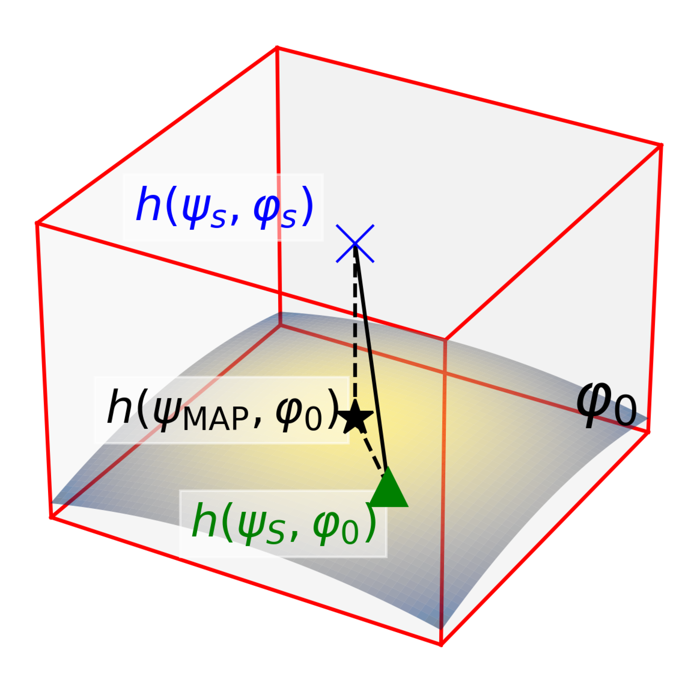
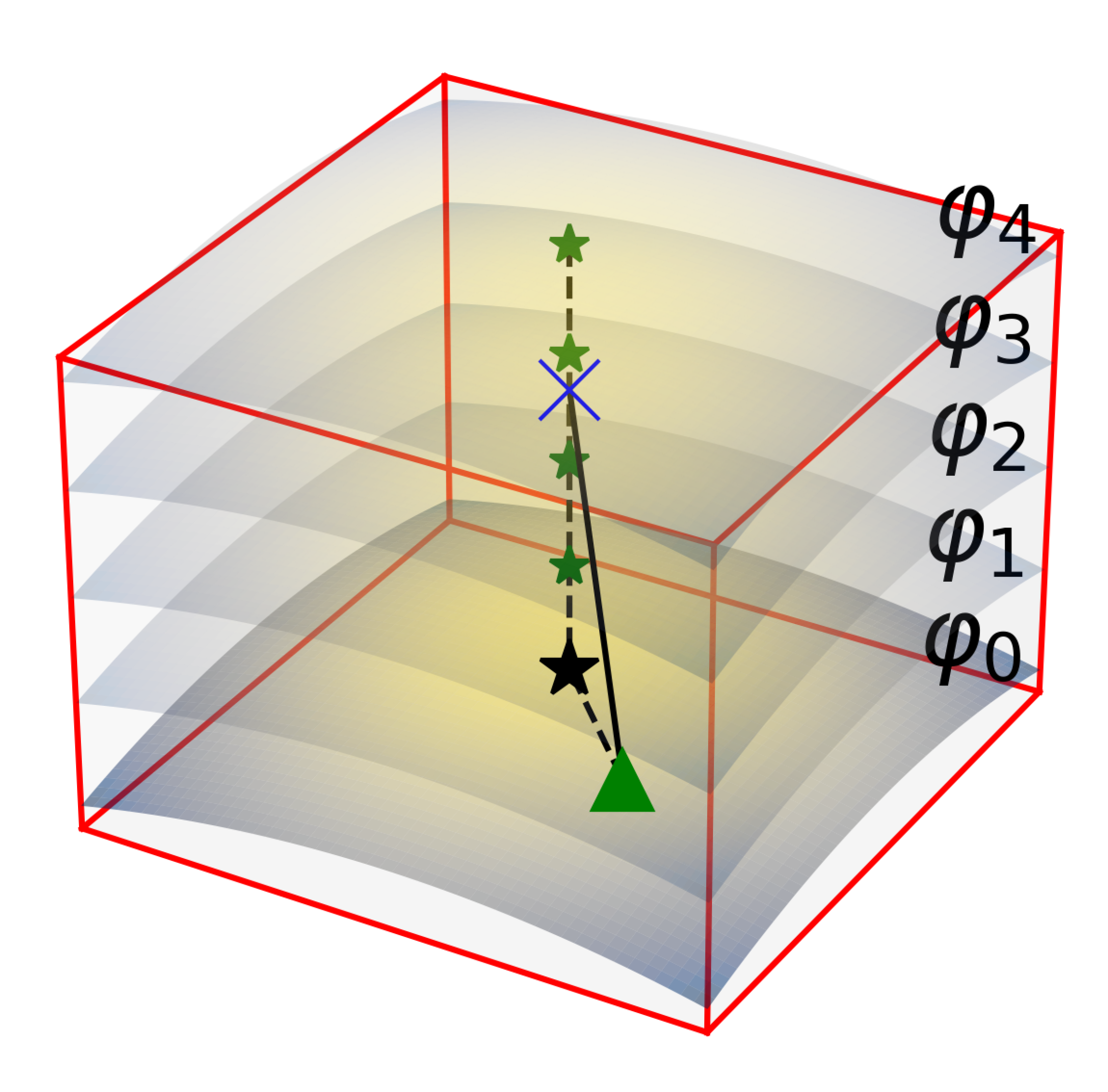
Figure 1: (Left panel) A schematic depicting an injected signal $h(\boldsymbol{\psi}_{s},\boldsymbol{\varphi}_{s})$ (blue cross) generated in the superset hypothesis $\mathcal{H}_{1}$ (red hypercube) inferred assuming the subset hypothesis $\mathcal{H}_{0}$ (shaded submanifold) where $\boldsymbol{\varphi}=\boldsymbol{\varphi}_{0}$ is fixed. The green triangle is the signal’s restriction to $\mathcal{H}_{0}$, and the black star is the inferred MAP $h(\boldsymbol{\psi}_{\rm MAP},\boldsymbol{\varphi}_{0})$. The two points do not coincide, representing inference biases. (Right panel) 5 samples (green and black stars) drawn by translating the MAP along the correction axis (vertical dashed line) constructed following Eqs. (17), (19).

III.2 Importance sampling formalism for the bias-corrected proposal

Given the set of samples $\{\boldsymbol{\psi}^{\prime},\boldsymbol{\varphi}^{\prime}\}\sim q(\boldsymbol{\psi}^{\prime},\boldsymbol{\varphi}^{\prime})$, the (unnormalized) importance weights are

$${w}_{ij} :=\frac{p(\boldsymbol{\psi}_{i}^{\prime},\boldsymbol{\varphi}_{j}^{\prime}|s,\mathcal{H}_{1})}{q(\boldsymbol{\psi}_{i}^{\prime},\boldsymbol{\varphi}_{j}^{\prime})}.~$$ (24)

Here, $p(\boldsymbol{\psi}^{\prime},\boldsymbol{\varphi}^{\prime}|s,\mathcal{H}_{1})$ is the target pdf, given by Bayes’ theorem as

$$p(\boldsymbol{\psi}^{\prime},\boldsymbol{\varphi}^{\prime}|s,\mathcal{H}_{1})=\frac{\mathcal{L}(\boldsymbol{\psi}^{\prime},\boldsymbol{\varphi}^{\prime}|s,\mathcal{H}_{1})\pi(\boldsymbol{\psi}^{\prime},\boldsymbol{\varphi}^{\prime}|\mathcal{H}_{1})}{\mathcal{Z}(s|\mathcal{H}_{1})}.$$ (25)

Following a similar push-forward argument as Eq. (23), we have

$$\pi(\boldsymbol{\psi}^{\prime},\boldsymbol{\varphi}^{\prime}|\mathcal{H}_{1}) =\pi(\boldsymbol{\psi},\boldsymbol{\varphi}|\mathcal{H}_{1})$$

$$=\pi(\boldsymbol{\psi}|\mathcal{H}_{0})\pi(\boldsymbol{\varphi}|\mathcal{H}_{1}).$$ (26)

Using Eqs. (23), (25), and (26), the importance weights (Eq. (24)) can thus be rewritten as

$$w_{ij}=\frac{\mathcal{L}(\boldsymbol{\psi}^{\prime}_{i},\boldsymbol{\varphi}^{\prime}_{j}|s,\mathcal{H}_{1})}{\mathcal{L}(\boldsymbol{\psi}_{i}|s,\mathcal{H}_{0})}.$$ (27)

Given the prior probability of obtaining $\boldsymbol{\varphi}=\boldsymbol{\varphi}_{0}$ in $\mathcal{H}_{1}$, $\pi(\boldsymbol{\varphi}=\boldsymbol{\varphi}_{0}|\mathcal{H}_{1})$, and the posterior probability $p(\boldsymbol{\varphi}=\boldsymbol{\varphi}_{0}|s,\mathcal{H}_{1})$ from Eqs. (24) and (27), the Savage-Dickey ratio can be straightforwardly evaluated following Eq. (15).

III.3 A more conservative proposal pdf based on a regularized normal approximation

The proposal constructed above aims to correct the induced inference biases through $\tau(\boldsymbol{\psi},\boldsymbol{\varphi})$ to maximize the overlap with the target pdf. However, the method strongly relies on the ability to accurately estimate the FIM at $\{\boldsymbol{\psi}_{\rm MAP},\boldsymbol{\varphi}_{0}\}$ in $\mathcal{H}_{1}$, which can be difficult if, e.g., the model parametrization is nearly “ill-posed”, such that the FIM is poorly-conditioned, increasing its susceptibility to numerical errors Vallisneri (2008). Here, we attempt to mitigate some of these technical challenges by constructing a more conservative proposal pdf, as described below.

We again treat as given the set of samples $\{\boldsymbol{\psi}\}|\mathcal{H}_{0}\sim p(\boldsymbol{\psi}|s,\mathcal{H}_{0})$. However, instead of randomly drawing $\boldsymbol{\varphi}\sim\pi(\boldsymbol{\varphi}|\mathcal{H}_{1})$, we deterministically choose $\boldsymbol{\varphi}=(\boldsymbol{\varphi}_{1},\ldots,\boldsymbol{\varphi}_{j},\ldots,\boldsymbol{\varphi}_{m})$ from a regular grid of size $m$ bounded by some range $[\boldsymbol{\varphi}_{\rm min},\boldsymbol{\varphi}_{\rm max}]$. The proposal is constructed in $m$ iterations, where at the $j^{\rm th}$ step, we first obtain the transformed set of samples $\boldsymbol{\theta}^{\prime}_{j}=\tau(\boldsymbol{\psi},\boldsymbol{\varphi}_{j})$ and calculate their posterior expectation $\bar{\boldsymbol{\theta}}^{\prime}_{j}:=\mathbb{E}[\boldsymbol{\theta}_{j}^{\prime}]$ by averaging. Then, $N$ samples of $(\boldsymbol{\psi}^{\prime}_{j},\boldsymbol{\varphi}^{\prime}_{j})$ are redrawn from a regularized normal approximation of the likelihood at $\bar{\boldsymbol{\theta}}_{j}^{\prime}$,

$$q_{j}(\boldsymbol{\psi}^{\prime},\boldsymbol{\varphi}^{\prime}):=\frac{|\Sigma_{\rm reg}|^{-1/2}}{(2\pi)^{d/2}}\exp[-\frac{1}{2}(\boldsymbol{\theta}^{\prime}-\bar{\boldsymbol{\theta}}^{\prime}_{j})^{T}\Sigma_{\rm reg}^{-1}(\boldsymbol{\theta}^{\prime}-\bar{\boldsymbol{\theta}}^{\prime}_{j})]$$ (28)

where

$$\Sigma_{\rm reg}:=\Gamma^{-1}+\epsilon\cdot D$$ (29)

is the regularized inverse of the FIM Tikhonov and Arsenin (1977); Hoerl and Kennard (1970) with $\epsilon>0$ some scalar regularization factor and $D$ a $d\times d$ diagonal matrix. We thus form a set of $N\times m$ samples $\{\boldsymbol{\psi}^{\prime},\boldsymbol{\varphi}^{\prime}\}:=\bigcup_{j}\{\boldsymbol{\psi}^{\prime}_{j},\boldsymbol{\varphi}^{\prime}_{j}\}$, which is distributed according to the mixture of all the regularized normal elements,

$$q_{\rm reg}(\boldsymbol{\psi}^{\prime},\boldsymbol{\varphi}^{\prime}):=\frac{1}{m}\sum_{j}q_{j}(\boldsymbol{\psi}^{\prime},\boldsymbol{\varphi}^{\prime}).$$ (30)

Here, the choice of $m$ is left as a free parameter of the method for a fair comparison with the basic implementation in the examples presented in the next section. It may also be informed, e.g., by the fractional coverage of the prior box by $\Sigma_{\rm reg}$ to ascertain sufficient overlap between consecutive $q_{j}$.

This choice of the proposal distribution assumes that the FIMs evaluated at the true signal point $(\boldsymbol{\psi}_{s},\boldsymbol{\varphi}_{s})|\mathcal{H}_{1}$ and the vacuum MAP point $(\boldsymbol{\psi}_{\rm MAP},\boldsymbol{\varphi}_{0})|\mathcal{H}_{1}$ are equal, which is consistent with the linear signal approximation Cutler and Vallisneri (2007); Kejriwal et al. (2024). We center the $j^{\rm th}$ proposal element $q_{j}$ at $\bar{\boldsymbol{\theta}}_{j}^{\prime}$ instead of the translated MAP ($\tau(\boldsymbol{\psi}_{\rm MAP},\boldsymbol{\varphi}_{j})$) since the sample mean is a more robust estimate of the MAP for the symmetric posteriors expected for high-SNR sources, and since the linear signal approximation fails for low-SNR asymmetric pdfs anyway. Furthermore, since $q_{j}$ is normally distributed, which is symmetric, it is reasonable to centre it at the mean of the translated samples. With the additional regularization step, we effectively introduce a noisy baseline to the inverse FIM elements to account for numerical uncertainties in its calculation and inversion.  We choose

$$\epsilon =\frac{|\Gamma\cdot\Gamma^{-1}|-1}{d}$$ (31)

$$D ={\rm diag}(\Gamma^{-1})$$ (32)

such that the noisy baseline scales with the inversion errors through $\epsilon$ and the uncertainties in the model parameters through $D$. The regularization step in Eq. (29) can be implemented iteratively, such that at the $k^{\rm th}$ iteration,

$$\Sigma_{{\rm reg},k} =\Gamma_{k-1}^{-1}+\epsilon_{k}\cdot D_{k}$$ (33)

where $\Gamma_{k}:=\Sigma_{{\rm reg},k}^{-1}$, $\Gamma_{0}\equiv\Gamma$, and

$$\epsilon_{k} :=\frac{|\Gamma_{k-1}\cdot\Gamma_{k-1}^{-1}|-1}{d}$$ (34)

$$D_{k} :={\rm diag}(\Gamma_{k-1}^{-1})$$ (35)

until the condition $\epsilon_{k}<\epsilon_{0}$ is met, where $\epsilon_{0}>0$ is a suitable error tolerance.

We present a schematic visualization of the practical implications of the regularized proposal in Figure 2, using only two parameters: the null hypothesis parameter $\psi$ along the x-axis and the additional superset hypothesis parameter $\varphi$ along the y-axis. The calculated correction axis (orange dashed line) is shown to deviate slightly from the true correction axis $(\psi_{s}-\psi_{\mathrm{MAP}},\varphi_{s}-\varphi_{0})$ (black dashed line) — this however is enough to inhibit sufficient overlap between the constructed proposals (green) and the target pdf (red) in the basic implementation, as shown in the top panel. In the regularized implementation with $\epsilon=10^{-2}$ and $D$ given by Eq. (32), the coverage of the same target pdf improves significantly as presented in the bottom panel. By construction, however, the regularized proposals also cover a larger “empty space” around the target distribution compared to the basic implementation, which may reduce the method’s importance efficiency $\eta$. This is consistent with the example results quoted in the next section, where the importance efficiency of the basic implementation was found to be factor $\sim 2-3$ higher than in the regularized framework.

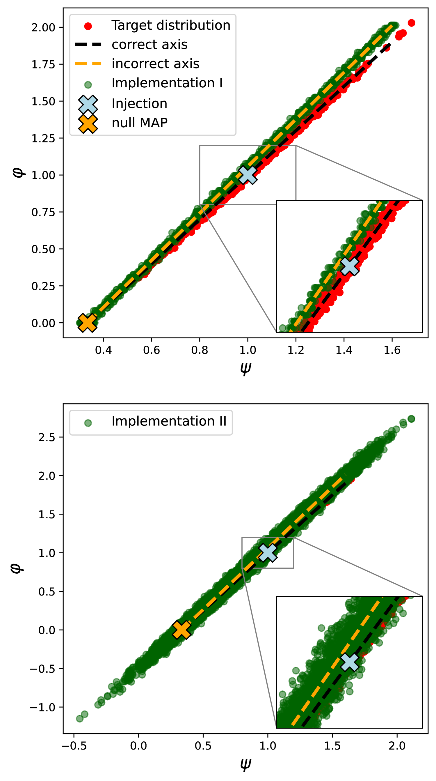
Figure 2: A 2D schematic with the subset hypothesis parameter $\psi$ along the x-axis and the superset hypothesis parameter $\varphi$ along the y-axis. The injection (blue cross) is recovered at the MAP (orange cross) with $\boldsymbol{\varphi}=0.0$ in the null hypothesis. We depict a case where the constructed correction axis (orange dashed line) deviates from the truth (black dashed line) due to computational errors. Draws from the target distribution are depicted in red and are overlayed by draws from the basic implementation (Sec. III.1, top panel) and the regularized implementation (Sec. III.3, bottom panel). The conservative proposals in the second method enable better coverage of the target, even when the correction axis is erroneous.

Given the set of proposed samples $(\boldsymbol{\psi}^{\prime},\boldsymbol{\varphi}^{\prime})\sim q_{\rm reg}(\boldsymbol{\psi}^{\prime},\boldsymbol{\varphi}^{\prime})$, the (unnormalized) importance weights are given following arguments from the previous section as

$$w_{{\rm reg},i} =\frac{p(\boldsymbol{\psi}^{\prime}_{i},\boldsymbol{\varphi}^{\prime}_{i}|s,\mathcal{H}_{1})}{q_{\rm reg}(\boldsymbol{\psi}^{\prime}_{i},\boldsymbol{\varphi}^{\prime}_{i})}.$$ (36)

Again, given the prior probability $\pi(\boldsymbol{\varphi}=\boldsymbol{\varphi}_{0}|\mathcal{H}_{1})$, and the posterior distribution $p(\boldsymbol{\varphi}=\boldsymbol{\varphi}_{0}|\mathcal{H}_{1})$ as the marginalization of $p(\boldsymbol{\psi}^{\prime},\boldsymbol{\varphi}^{\prime}|s,\mathcal{H}_{1})$ over $\boldsymbol{\psi}^{\prime}$ evaluated at $\boldsymbol{\varphi}_{0}$, we obtain the Savage-Dickey ratio following Eq. (15).

IV Examples

IV.1 Setup

Waveform model — We now present example results contextualizing the two bias-corrected techniques—the basic and regularized implementations—for LISA EMRIs. The injected signal $s$ is modeled as a fully relativistic adiabatic Kerr EMRI Pound and Wardell (2021) evolving in a circular-equatorial orbit, implemented by Khalvati et al. Khalvati et al. (2024) in the modular framework of the FastEMRIWaveforms (FEW) package Katz et al. (2021); Chua et al. (2021). It is described by 10 vacuum-GR parameters: the redshifted masses, $M$, $\mu$, of the MBH and CO respectively, the dimensionless spin of the MBH, $a$, the initial semi-latus rectum of the orbit, $p_{0}$, the initial azimuthal phase, $\Phi_{0}$, and extrinsic parameters $D_{L},(\theta_{S},\phi_{S}),(\theta_{K},\phi_{K})$, i.e. the source’s luminosity distance, sky location, and the MBH’s spin orientation to the solar system, respectively. The true source additionally incorporates the planetary migration effect due to an accretion disk surrounding the MBH, which can be modeled as a secular power-law perturbation modifying the flux balance laws of the EMRI evolution as Kocsis et al. (2011); Barausse et al. (2014); Speri et al. (2023)

$$\dot{L}=\dot{L}_{\rm GR}\left(1+A\left(\frac{p}{10M}\right)^{n_{r}}\right)$$ (37)

where $\dot{L}_{\rm GR}$ is the axial component of the angular momentum flux in vacuum-GR calculated at leading order, $p$ is the semi-latus rectum of the instantaneous orbit, and $(A,n_{r})$ are 2 new parameters that describe the disk effect. In the following examples, the accretion + vacuum-GR evolution with variable $A$ (and some fixed $n_{r}$) characterizes the superset beyond vacuum-GR hypothesis ($\mathcal{H}_{1}$), and $A=0$ is fixed in the subset vacuum-GR hypothesis ($\mathcal{H}_{0}$).

Data analysis setup — We asuume flat priors on all model parameters such that the posterior is proportional to the likelihood and the MAP is equal to the maximum likelihood estimate (MLE). We sample from the various posteriors in our study using Eryn, a Bayesian inference package designed for LISA Karnesis et al. (2023). It incorporates parallel tempering useful for inferring biased MAPs, and interfaces with LISAanalysistools (LAT) Katz et al. (2024a) and fastlisaresponse Katz et al. (2022) utility packages, providing consistent and modular integration with GW data analysis tools and LISA noise models. To accurately calculate the FIM at the MLE, required for the transformation function, we employ the StableEMRIFishers (SEF) Kejriwal et al. (tion) package that systematically calculates numerical waveform derivatives and hence the FIM, enhancing its stability.

In all the following examples, we work in the log-mass parametrization $(M,\mu)\to(\ln M,\ln\mu)$, which reduces the ill-posedness of the model, and choose $M=10^{6}M_{\odot}$, $\mu=50M_{\odot}$, $a=0.9$, $\Phi_{0}=1.0$, $(\theta_{S},\phi_{S})=(\pi/4,\pi/3)$, and $(\theta_{K},\phi_{K})=(\pi/6,\pi/5)$ in the true signal. We additionally fix $n_{r}=8$ corresponding to the inner region of a typical AGN disk Kocsis et al. (2011); Speri et al. (2023). $p_{0}$ is chosen for the EMRI to plunge at the end of the 1-year observation window, and $D_{L}$ such that the source’s signal-to-noise ratio (SNR) $\rho:=\langle s|s\rangle^{1/2}=100$. Bayesian inference is performed with 8 MCMC walkers across 3 temperatures within a reasonable prior hypercube (flat, bounded priors) centered at the injected signal parameters. Finally, given the injected parameter vector $\hat{\boldsymbol{\psi}}$, the mean of the MCMC samples from the subset hypothesis, $\bar{\boldsymbol{\psi}}_{{\rm sub}}$, and the corresponding mean of the importance samples in the superset hypothesis, $\bar{\boldsymbol{\psi}}_{{\rm sup}}$ (Eqs. (5) and (27)), we define

$$r_{i}:=\frac{|\hat{\boldsymbol{\psi}}_{i}-\bar{\boldsymbol{\psi}}_{{\rm sub},i}|}{|\hat{\boldsymbol{\psi}}_{i}-\bar{\boldsymbol{\psi}}_{{\rm sup},i}|}$$ (38)

as a measure of the fractional change in the point estimate of $\boldsymbol{\psi}$. $r_{i}>1$ corresponds to an improved (closer to the injection) expectation value of the $i^{\rm th}$ model parameter after the procedure.

IV.2 Example i@: Intrinsic parameters only

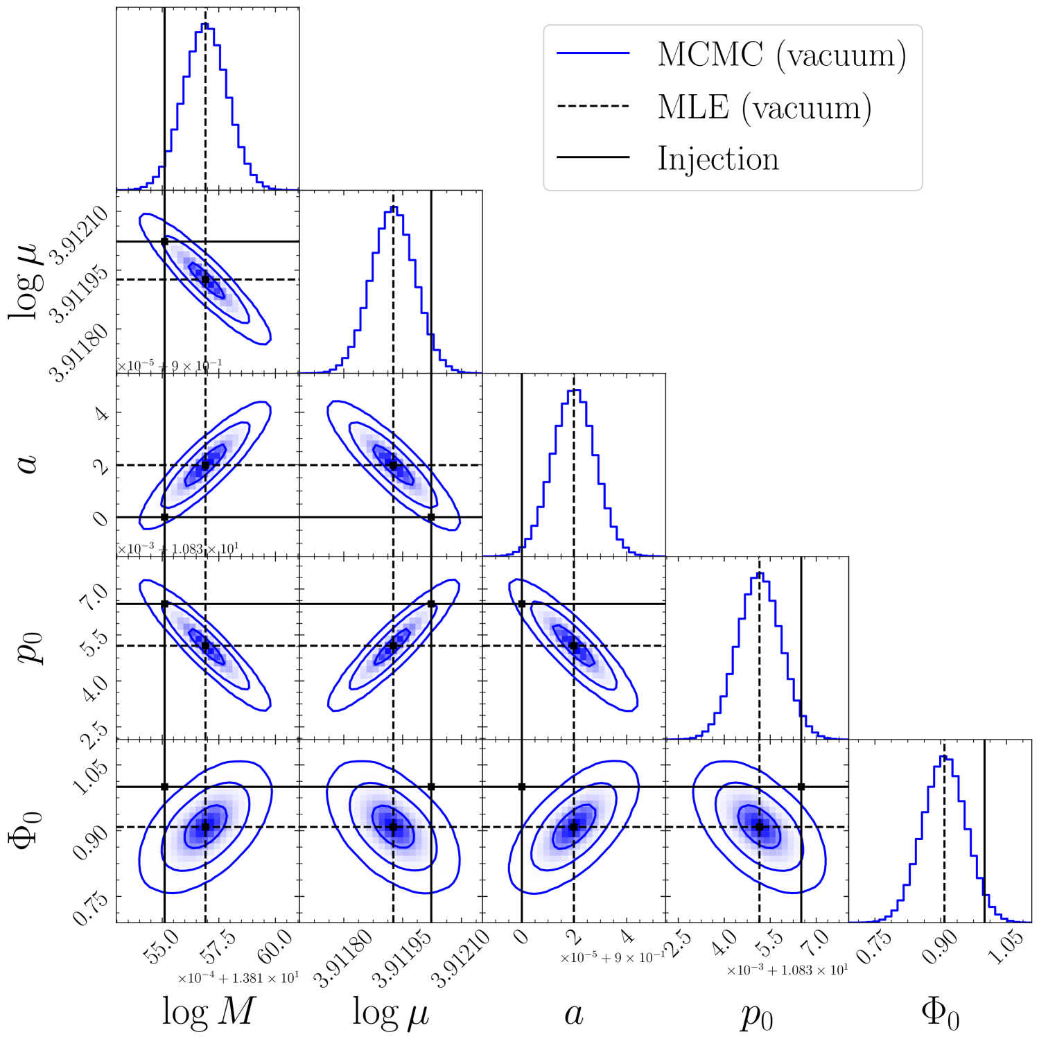
Figure 3: Distribution of posterior samples of an EMRI signal assuming the vacuum-GR (subset) hypothesis $\mathcal{H}_{0}$ with model parameters $\boldsymbol{\psi}=(\ln M,\ln\mu,a,p_{0},\Phi_{0})$ (blue contours). The injected signal exhibits an additional beyond vacuum-GR parameter $\boldsymbol{\varphi}=A=1.92\times 10^{-5}$ induced by the effect of an accretion disk around the MBH. The recovered MLE $\boldsymbol{\psi}_{\rm MLE}|\mathcal{H}_{0}$ (dashed line) is $\sim 2\sigma$ biased to the injected parameters (solid line).

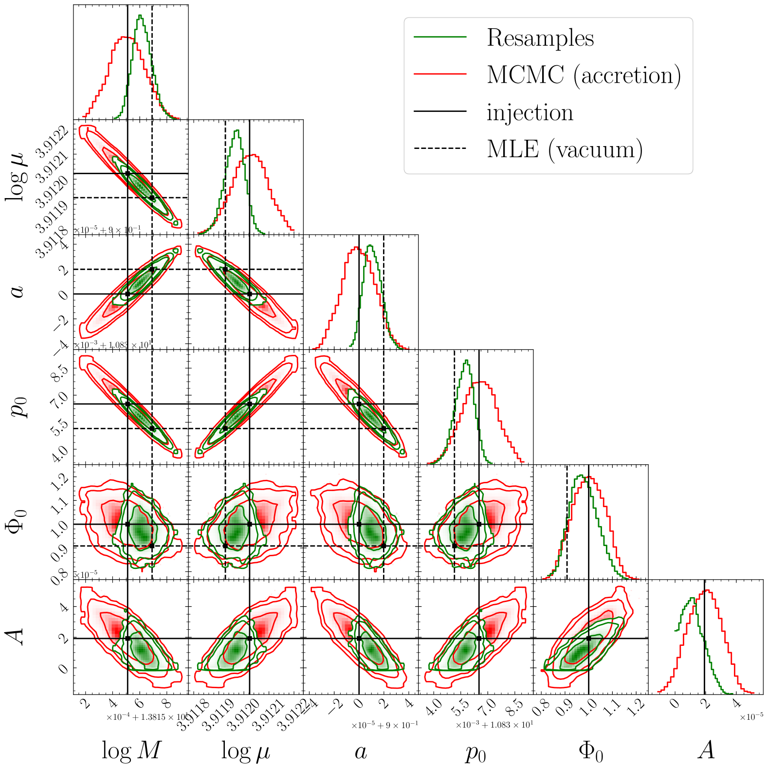
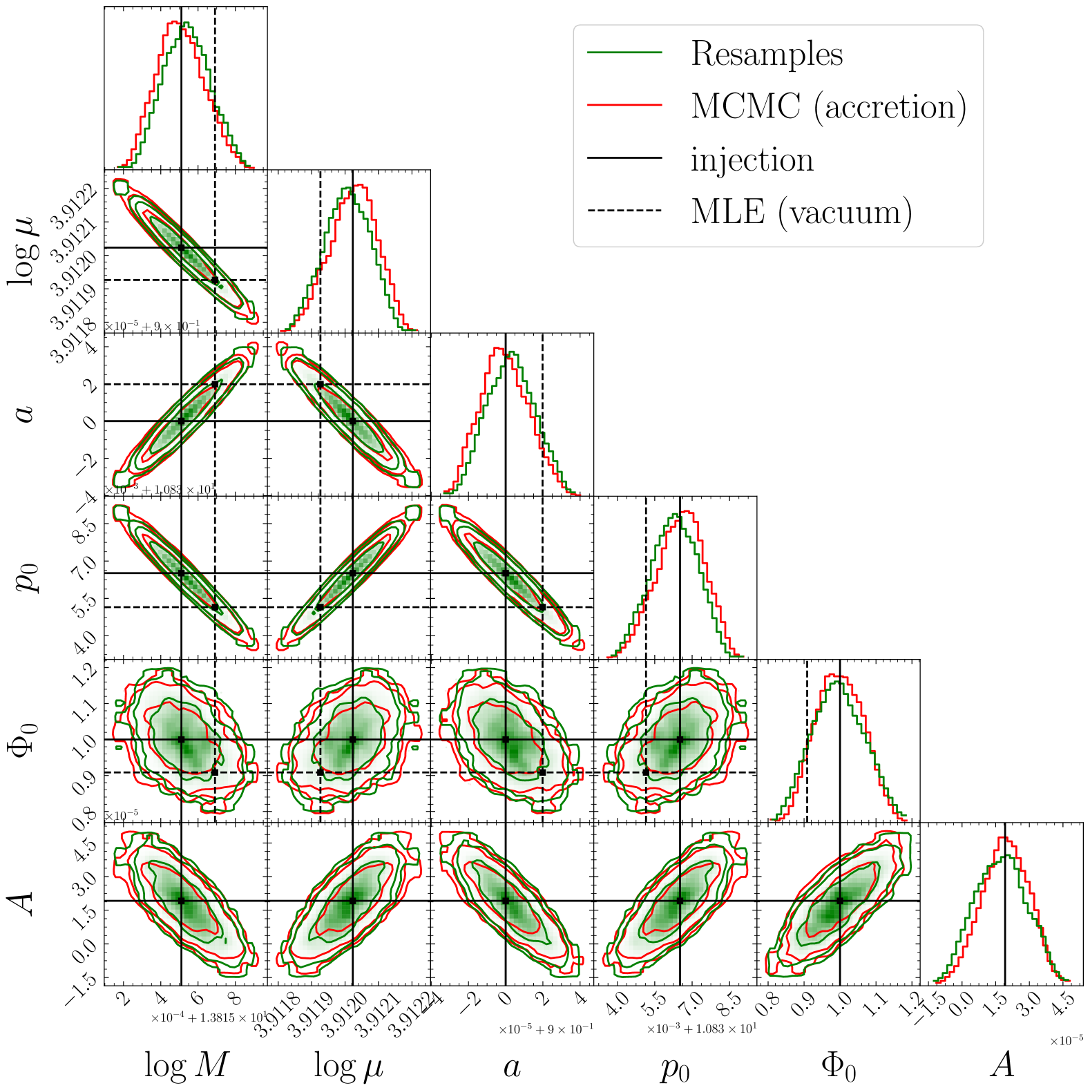
Figure 4: Distribution of bias-corrected importance resamples (green contours) in Example i@ in the basic implementation (section III.1, top panel) and regularized implementation (section III.3, bottom panel), overlayed with posterior samples of the injected EMRI signal in the true beyond vacuum-GR (superset) hypothesis $\mathcal{H}_{1}$ (red contours).

In the first example, all extrinsic parameters are fixed, i.e., only the parameter set $\boldsymbol{\psi}:=(\ln M,\ln\mu,a,p_{0},\Phi_{0})$ is inferred in the subset hypothesis. The superset hypothesis includes the additional parameter $\boldsymbol{\varphi}:=(A)$, with injection value $A=1.92\times 10^{-5}$. In the subset hypothesis, we generate $\approx 9\times 10^{5}$ total samples $\boldsymbol{\psi}|\mathcal{H}_{0}\sim\mathcal{L}(\boldsymbol{\psi}|s,\mathcal{H}_{0})$ centered at the $\sim 2\sigma$ biased vacuum-GR MLE $\boldsymbol{\psi}_{\rm MLE}|\mathcal{H}_{0}$ with respect to the injection. As shown in the corner plot in Fig. 3, the distribution of these samples poorly overlaps with the injected signal parameters, especially along $a$ and $\Phi_{0}$, rendering standard importance sampling (i.e., with $\tau=I$) infeasible, and motivating the bias-correction procedure outlined above. We set the prior range on $A$ as $[A_{\rm min},A_{\rm max}]=[0.0,1.0]\times 10^{-4}$, the size $N$ of samples in the subset hypothesis equal to the final $1\%$ of the MCMC samples, and fix $m=5$, for a total of $N\times m\approx 5\times 10^{4}$ samples of $(\boldsymbol{\psi},\boldsymbol{\varphi})$. The number of discarded samples and choice of $m$ were empirically made to ensure a sufficient (but not excessive, for computational feasibility) set of proposal samples. Furthermore, we approximate the vacuum-GR MLE as $\boldsymbol{\psi}_{\rm MLE}\approx\mathbbm{E}[\boldsymbol{\psi}_{<3\sigma}|\mathcal{H}_{0}]$ where $\boldsymbol{\psi}_{<3\sigma}|\mathcal{H}_{0}$ is the set of vacuum-GR MCMC samples within $3\sigma$ of the MLE, which is correspondingly the set of $99.7\%$ of samples with the highest likelihood values. The mean of a finite set of samples provides a more robust estimate of the MLE than the inferred MLE point for symmetric likelihood surfaces, as expected for high-SNR sources as in this example (see Fig. 3). Additionally, by only considering samples within $3\sigma$ of the MLE point, we ensure that any tail asymmetries in the sampling do not bias the estimate. Finally, the FIM is calculated at $(\boldsymbol{\psi}_{\rm MLE},\boldsymbol{\varphi}_{0})|\mathcal{H}_{1}$.

In the basic implementation, samples of $\boldsymbol{\varphi}\equiv A$ are drawn uniformly from its prior range and pairs of $(\boldsymbol{\psi},\boldsymbol{\varphi})$ are transformed using $\tau$ (Eq. (19)) to obtain the bias-corrected samples $\{\boldsymbol{\psi}^{\prime},\boldsymbol{\varphi}^{\prime}\}\sim q(\boldsymbol{\psi}^{\prime},\boldsymbol{\varphi}^{\prime})$, with the proposal distribution $q(\boldsymbol{\psi}^{\prime},\boldsymbol{\varphi}^{\prime})$ given by Eq. (23) (with $\pi(\boldsymbol{\psi}|\mathcal{H}_{0})\propto 1$). The importance resampled means of the vacuum-GR parameters are calculated following Eqs. (5) and (27) such that the fractional change $r_{i}$ defined in Eq. (38) is $\sim$ 2-3 for all parameters. Simultaneously, the sample mean of the beyond vacuum-GR parameter $\boldsymbol{\varphi}$ is within 35% of the injection. From Eqs. (6) and (8), the importance sampling efficiency is $\eta\approx 0.08$, typical of the importance sampling class of methods for high SNR sources (see, e.g., Romero-Shaw et al. (2021) and Saleh et al. (2024)). The Savage-Dickey ratio, calculated from Eq. (15) is $\mathcal{B}_{0}^{1}\approx 2.0$ in favor of the superset beyond vacuum-GR hypothesis. Finally, we obtain the reweighted importance distribution by drawing $N_{\rm ess}$ samples without replacement from the set of proposed samples in proportion to their weights. The importance resamples are plotted in the top panel of Fig. 4, overlayed with $\approx 5\times 10^{5}$ MCMC samples from the posterior in the true (superset) hypothesis $\mathcal{H}_{1}$ for comparison. Notably, the coverage is partial, showcasing a setback of the basic implementation for posterior recovery. This could result from numerical errors in the calculation or inversion of the FIM, which is especially likely for the ill-posed (highly correlated) EMRI parametrization, or if the vacuum-GR MLE estimator is incorrect, etc. (see Fig. 2 and discussion in Sec. III.3).

Addressing such errors in the basic implementation is difficult, particularly without prior knowledge of the true posterior distribution, prompting a switch to the more conservative regularized implementation. Here, $A$ is chosen from a linear grid of $m=5$ values on the prior range, and $\Sigma_{\rm reg}$ is obtained from Eqs. (29), (31)-(35), implemented iteratively until $\epsilon_{k}<\epsilon_{0}=10^{-12}$. Then, samples $\{\boldsymbol{\psi}^{\prime},\boldsymbol{\varphi}^{\prime}\}\sim q_{\rm reg}(\boldsymbol{\psi}^{\prime},\boldsymbol{\varphi}^{\prime})$ are generated following section III.3. The importance expectations on the vacuum-GR parameters can be calculated from the sample likelihoods, such that $r_{i}$ (Eq. (38)) is now $\sim 10$ for all parameters, much higher than $r_{i}$ in the basic implementation. The beyond vacuum-GR parameter is also recovered within $7.5\%$ of the injection. In contrast, the importance sampling efficiency is lower, but is still $\eta\approx 0.05$. This is expected since the regularized proposal pdf is broader by construction, covering a larger “empty” region around the true posterior. The Savage-Dickey ratio in the regularized implementation is $\mathcal{B}_{0}^{1}\approx 1.7$, which is consistent with the basic implementation for model selection, within sampling uncertainties. We also recover an improved coverage of the posterior pdf, as shown in the bottom panel of Fig. 4. Thus, despite the lower importance efficiency, importance sampling under the regularized framework provides an overall improved inference of the target distribution.

IV.3 Example ii@: Additional parameters

The extrinsic parameters are restored in the second example, as would be the case in more realistic analyses. Here, $\boldsymbol{\psi}:=(\ln M,\ln\mu,a,p_{0},\Phi_{0},D_{L},\theta_{S},\phi_{S},\theta_{K},\phi_{K})$ and $\boldsymbol{\varphi}:=A$ with true value $A=3.84\times 10^{-5}$ in the signal. The perturbative effect amplitude is doubled to induce a similarly large $\sim 2\sigma$ bias on the parameters for a fair comparison (see Fig. 5 of Appendix A for the full posterior corner plot). Again, discarding the first $99\%$ of the $\approx 1.3\times 10^{6}$ total MCMC samples in $\mathcal{H}_{0}$, and setting $m=5$, we use $N\times m\approx 6.5\times 10^{4}$ vacuum-GR samples in the inference. The prior range on $A$ is unchanged.

In the basic implementation, calculating the importance expectation on $\boldsymbol{\psi}$, the fractional change $r_{i}$ (Eq. (38)) is $\sim 2$–$5$, with the sample mean of $\boldsymbol{\varphi}$ within $15\%$ of the injection. The importance efficiency is $\approx 0.05$, and the importance resamples still poorly overlap with the true posterior in the superset beyond vacuum-GR hypothesis. The Savage-Dickey ratio is obtained following Eq. (15) as $\mathcal{B}_{0}^{1}\approx 1.7$. In the regularized implementation, the importance samples for the same injection provide $r_{i}$ for $\boldsymbol{\psi}$ of the order $\sim 10-100$, and the beyond vacuum-GR parameter $\boldsymbol{\varphi}$ is recovered within $5\%$ of the injected value. However, the importance efficiency drops to $\approx 0.01$ because of the coverage of a larger empty space in the added dimensions. The Savage-Dickey ratio in the regularized scheme is $\mathcal{B}_{0}^{1}\approx 1.83$, again consistent with the basic implementation for model selection. The importance resamples strongly overlap with MCMC samples drawn from the posterior pdf in the true (superset) hypothesis, as shown in Fig. 6 in the Appendix.

V Discussion

V.1 Summary and outlook

While dynamic inference methods like MCMC are widely employed in GW data analysis, they may become computationally infeasible for the inference and comparison of alternate hypotheses in a nested framework, which includes the general class of perturbative beyond vacuum-GR effects in binary GW sources. In this paper, we presented the bias-corrected importance sampling formalism and describe two implementations—basic and regularized—targeting the efficient inference of such effects. Empirically, we found that redoing MCMC inference of the posterior surface in the superset hypothesis required an order-of-magnitude more calls to the likelihood function than needed for bias-corrected importance sampling. Additionally, since all samples from the proposal pdf are simultaneously available in importance sampling, likelihood calls can be made parallelly. This is an inherent limitation of sequential techniques like MCMC and nested sampling. In other words, the bias-corrected importance sampling method enables the inference of $\gtrsim$ an order-of-magnitude more alternate nested hypotheses compared to methods like MCMC at the same computational expense; this is especially relevant, e.g., for high-precision probes of strong gravity sources in galactic centers like EMRIs and MBHBs, future observations Gupta et al. (2024) of which may be used to perform multiple different tests of astrophysical and modified-GR theories.

While the basic implementation underscores fundamental aspects of the bias-corrected importance sampling framework, the method heavily relies on the accuracy of the correction axis constructed following Eq. (19), which is susceptible to both theoretical and numerical errors, i.e., if the linear bias approximation (Eq. (17)) is invalid or components thereof are incorrectly computed. In our examples, this translated to poor overlap of the importance resamples with the true posterior. The more conservative proposal defined in the regularized implementation was found to be relatively robust, providing better overall inference of the underlying posterior. Alternatively, a better-posed EMRI parametrization that promotes more stable results may resolve some of these practical challenges and will be explored in a separate work. Finally, we stress that our formalism is not restricted to nested model setups, and can be generically applied to infer bias-corrected targets by suitably replacing the transformation function (Eq. (19)).

V.2 Future directions

The mathematical framework developed in section III generically applies to any number of induced beyond vacuum-GR effects, each with an arbitrary number of model parameters. As argued in Kejriwal et al. (2024), multiple such effects may be present in the signal simultaneously, motivating a joint inference analysis. Such combinations of beyond vacuum-GR effects can be readily studied in follow-up work under the bias-corrected framework. Similarly, model-agnostic tests of GR (developed, e.g., in the ppE formalism Yunes and Pretorius (2009), or for parametrized tests of GR with observations from ground-based detectors Li et al. (2012); Saleem et al. (2022)) may be defined as the superset model and studied inexpensively in our framework. However, their parametric approach with non-physical degrees of freedom has been previously challenged Chua and Vallisneri (2020).

The global-fit pipeline, adopted as the primary inference pipeline for LISA data analysis Vallisneri (2009); Littenberg and Cornish (2023); Katz et al. (2024b), aims to simultaneously infer all sources in the data stream through techniques like reversible-jump MCMC Green (1995) and blocked Gibbs sampling Gelfand and Smith (1990); Liu (2008). In such a setup, inferring beyond vacuum-GR effects using conventional methods may not even be feasible, since the introduction of a single beyond vacuum-GR effect with dimensionality $d_{\boldsymbol{\varphi}}$ would require a new global-fit on a posterior space with $S\times d_{\boldsymbol{\varphi}}$ additional dimensions, where $S$ is the number of detected sources. Alternatively, given only the vacuum-GR posteriors as the output of the global-fit analysis, our framework can readily construct proposals spanning the underlying posteriors in the beyond vacuum-GR hypothesis, feasibly infer them, and even inform the global-fit pipeline as a consequence — allowing robust and systematic inference of perturbative beyond vacuum-GR effects in GW sources in the future.

Appendix A Example ii@ corner plots

In Fig. 5, we present the full 10-dimensional posterior distribution obtained via the MCMC inference of the injected signal in Example ii@ assuming the vacuum-GR hypothesis. We show the corresponding importance resamples for the regularized bias-corrected importance sampling implementation in Fig. 6, overlaid with MCMC samples from the posterior pdf in the true (superset) hypothesis.

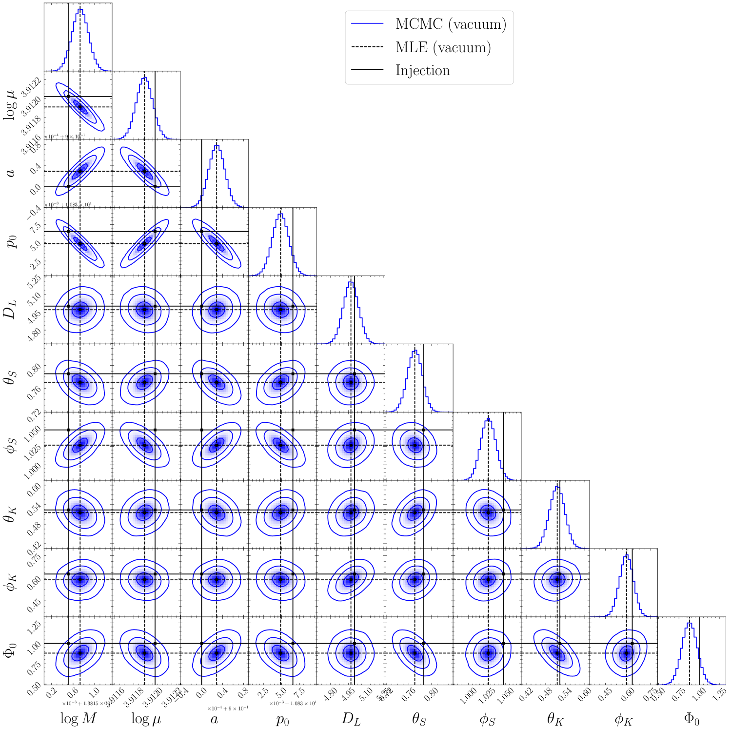
Figure 5: Distribution of posterior samples of an EMRI signal assuming the vacuum-GR (subset) hypothesis $\mathcal{H}_{0}$ with model parameters $\boldsymbol{\psi}=(\ln M,\ln\mu,a,p_{0},\Phi_{0},D_{L},\theta_{S},\phi_{S},\theta_{K},\phi_{K})$ (blue contours). The injected signal (solid line) includes an additional beyond vacuum-GR parameter $\boldsymbol{\varphi}=A=3.84\times 10^{-5}$ induced by the effect of an accretion disk around the MBH. The recovered MLE $\boldsymbol{\psi}_{\rm MLE}|\mathcal{H}_{0}$ (dashed line) is $\sim 2\sigma$ biased to the injection for all parameters except $(D_{L},\theta_{K},\phi_{K})$.

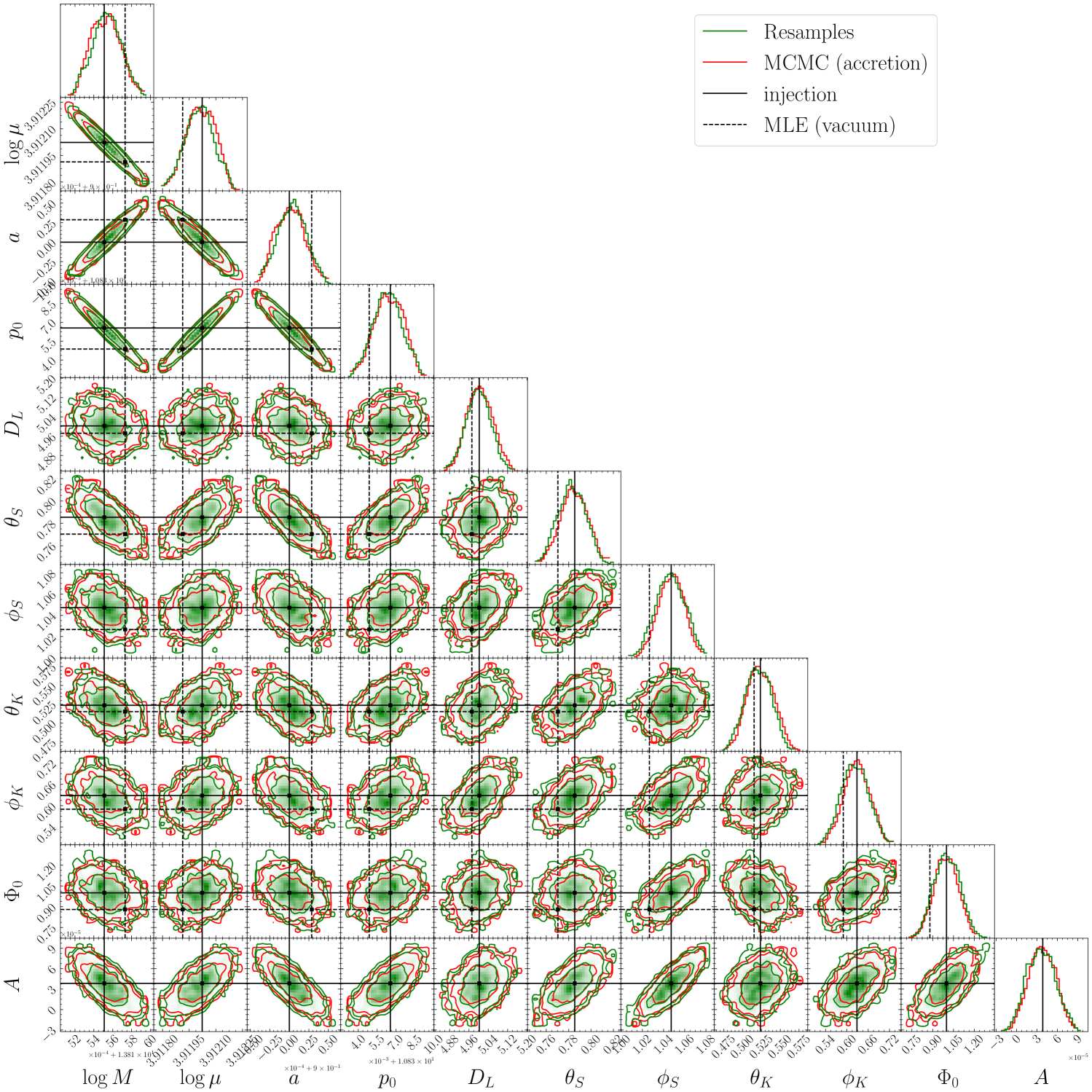
Figure 6: Distribution of bias-corrected importance resamples (green contours) in the regularized implementation of Example ii@, overlaid with posterior samples of the injected EMRI signal in the true beyond vacuum-GR (superset) hypothesis $\mathcal{H}_{1}$ (red contours).

References

- Amaro-Seoane et al. (2017) P. Amaro-Seoane et al. (LISA), (2017), arXiv:1702.00786 [astro-ph.IM] .
- Seoane et al. (2023) P. A. Seoane et al. (LISA), Living Rev. Rel. 26, 2 (2023), arXiv:2203.06016 [gr-qc] .
- Colpi et al. (2024) M. Colpi et al., (2024), arXiv:2402.07571 [astro-ph.CO] .
- Barack and Cutler (2004) L. Barack and C. Cutler, Phys. Rev. D 69, 082005 (2004), arXiv:gr-qc/0310125 .
- Babak et al. (2017) S. Babak, J. Gair, A. Sesana, E. Barausse, C. F. Sopuerta, C. P. L. Berry, E. Berti, P. Amaro-Seoane, A. Petiteau, and A. Klein, Phys. Rev. D 95, 103012 (2017), arXiv:1703.09722 [gr-qc] .
- Berry et al. (2019) C. P. L. Berry, S. A. Hughes, C. F. Sopuerta, A. J. K. Chua, A. Heffernan, K. Holley-Bockelmann, D. P. Mihaylov, M. C. Miller, and A. Sesana, (2019), arXiv:1903.03686 [astro-ph.HE] .
- Yunes and Pretorius (2009) N. Yunes and F. Pretorius, Phys. Rev. D 80, 122003 (2009), arXiv:0909.3328 [gr-qc] .
- Barausse et al. (2016) E. Barausse, N. Yunes, and K. Chamberlain, Phys. Rev. Lett. 116, 241104 (2016), arXiv:1603.04075 [gr-qc] .
- Arun et al. (2022) K. G. Arun et al. (LISA), Living Rev. Rel. 25, 4 (2022), arXiv:2205.01597 [gr-qc] .
- Speri et al. (2024) L. Speri, S. Barsanti, A. Maselli, T. P. Sotiriou, N. Warburton, M. van de Meent, A. J. K. Chua, O. Burke, and J. Gair, (2024), arXiv:2406.07607 [gr-qc] .
- Barausse et al. (2014) E. Barausse, V. Cardoso, and P. Pani, Phys. Rev. D 89, 104059 (2014), arXiv:1404.7149 [gr-qc] .
- Speri et al. (2023) L. Speri, A. Antonelli, L. Sberna, S. Babak, E. Barausse, J. R. Gair, and M. L. Katz, Phys. Rev. X 13, 021035 (2023), arXiv:2207.10086 [gr-qc] .
- Kocsis et al. (2011) B. Kocsis, N. Yunes, and A. Loeb, Phys. Rev. D 84, 024032 (2011), arXiv:1104.2322 [astro-ph.GA] .
- Garg et al. (2024a) M. Garg, L. Sberna, L. Speri, F. Duque, and J. Gair, (2024a), arXiv:2410.02910 [astro-ph.GA] .
- Duque et al. (2024) F. Duque, S. Kejriwal, L. Sberna, L. Speri, and J. Gair, (2024), arXiv:2411.03436 [gr-qc] .
- Favata (2014) M. Favata, Phys. Rev. Lett. 112, 101101 (2014), arXiv:1310.8288 [gr-qc] .
- Romero-Shaw et al. (2020) I. M. Romero-Shaw, P. D. Lasky, E. Thrane, and J. C. Bustillo, Astrophys. J. Lett. 903, L5 (2020), arXiv:2009.04771 [astro-ph.HE] .
- Romero-Shaw et al. (2021) I. M. Romero-Shaw, P. D. Lasky, and E. Thrane, Astrophys. J. Lett. 921, L31 (2021), arXiv:2108.01284 [astro-ph.HE] .
- Piovano et al. (2020) G. A. Piovano, A. Maselli, and P. Pani, Phys. Rev. D 102, 024041 (2020), arXiv:2004.02654 [gr-qc] .
- Mathews et al. (2022) J. Mathews, A. Pound, and B. Wardell, Phys. Rev. D 105, 084031 (2022), arXiv:2112.13069 [gr-qc] .
- Skoupý and Witzany (2024) V. Skoupý and V. Witzany, (2024), arXiv:2411.16855 [gr-qc] .
- Lyu et al. (2024) Z. Lyu, Z. Pan, J. Mao, N. Jiang, and H. Yang, (2024), arXiv:2501.03252 [astro-ph.HE] .
- Hinderer and Flanagan (2008) T. Hinderer and E. E. Flanagan, Phys. Rev. D 78, 064028 (2008), arXiv:0805.3337 [gr-qc] .
- Barack and Pound (2019) L. Barack and A. Pound, Rept. Prog. Phys. 82, 016904 (2019), arXiv:1805.10385 [gr-qc] .
- Pound and Wardell (2021) A. Pound and B. Wardell, (2021), 10.1007/978-981-15-4702-7_38-1, arXiv:2101.04592 [gr-qc] .
- Fujita and Shibata (2020) R. Fujita and M. Shibata, Phys. Rev. D 102, 064005 (2020), arXiv:2008.13554 [gr-qc] .
- Isoyama et al. (2022) S. Isoyama, R. Fujita, A. J. K. Chua, H. Nakano, A. Pound, and N. Sago, Phys. Rev. Lett. 128, 231101 (2022), arXiv:2111.05288 [gr-qc] .
- Hughes et al. (2021) S. A. Hughes, N. Warburton, G. Khanna, A. J. K. Chua, and M. L. Katz, Phys. Rev. D 103, 104014 (2021), [Erratum: Phys.Rev.D 107, 089901 (2023)], arXiv:2102.02713 [gr-qc] .
- Kejriwal et al. (2024) S. Kejriwal, L. Speri, and A. J. K. Chua, Phys. Rev. D 110, 084060 (2024), arXiv:2312.13028 [gr-qc] .
- Robert and Casella (2004) C. Robert and G. Casella, Monte Carlo statistical methods (Springer Verlag, 2004).
- Skilling (2006) J. Skilling, Bayesian Analysis 1, 833 (2006).
- Higson et al. (2019) E. Higson, W. Handley, M. Hobson, and A. Lasenby, Statistics and Computing 29, 891 (2019), arXiv:1704.03459 [stat.CO] .
- Cutler and Vallisneri (2007) C. Cutler and M. Vallisneri, Phys. Rev. D 76, 104018 (2007), arXiv:0707.2982 [gr-qc] .
- Abbott et al. (2016) B. P. Abbott et al. (LIGO Scientific, Virgo), Phys. Rev. Lett. 116, 221101 (2016), [Erratum: Phys.Rev.Lett. 121, 129902 (2018)], arXiv:1602.03841 [gr-qc] .
- Agazie et al. (2023a) G. Agazie et al. (NANOGrav), Astrophys. J. Lett. 951, L50 (2023a), arXiv:2306.16222 [astro-ph.HE] .
- Gelman et al. (2004) A. Gelman, J. B. Carlin, H. S. Stern, and D. B. Rubin, Bayesian Data Analysis, 2nd ed. (Chapman and Hall/CRC, 2004).
- Li (2004) K.-H. Li, “The sampling/importance resampling algorithm,” in Applied Bayesian Modeling and Causal Inference from Incomplete-Data Perspectives (John Wiley & Sons, Ltd, 2004) Chap. 24, pp. 265–276, https://onlinelibrary.wiley.com/doi/pdf/10.1002/0470090456.ch24 .
- Jaynes (2003) E. T. Jaynes, Probability theory: The logic of science (Cambridge University Press, Cambridge, 2003).
- Finn (1992) L. S. Finn, Phys. Rev. D 46, 5236 (1992), arXiv:gr-qc/9209010 .
- Cutler and Flanagan (1994) C. Cutler and E. E. Flanagan, Phys. Rev. D 49, 2658 (1994), arXiv:gr-qc/9402014 .
- Abbott et al. (2019) B. P. Abbott et al. (LIGO Scientific, Virgo), Phys. Rev. D 100, 104036 (2019), arXiv:1903.04467 [gr-qc] .
- Abbott et al. (2021a) R. Abbott et al. (LIGO Scientific, Virgo), Phys. Rev. D 103, 122002 (2021a), arXiv:2010.14529 [gr-qc] .
- Abbott et al. (2021b) R. Abbott et al. (LIGO Scientific, VIRGO, KAGRA), (2021b), arXiv:2112.06861 [gr-qc] .
- Agazie et al. (2023b) G. Agazie et al. (NANOGrav), Astrophys. J. Lett. 951, L8 (2023b), arXiv:2306.16213 [astro-ph.HE] .
- Johnson et al. (2024) A. D. Johnson et al. (NANOGrav), Phys. Rev. D 109, 103012 (2024), arXiv:2306.16223 [astro-ph.HE] .
- Smarra et al. (2023) C. Smarra et al. (European Pulsar Timing Array), Phys. Rev. Lett. 131, 171001 (2023), arXiv:2306.16228 [astro-ph.HE] .
- Antoniadis et al. (2023) J. Antoniadis et al. (EPTA, InPTA:), Astron. Astrophys. 678, A50 (2023), arXiv:2306.16214 [astro-ph.HE] .
- Quelquejay Leclere et al. (2023) H. Quelquejay Leclere et al. (European Pulsar Timing Array, EPTA), Phys. Rev. D 108, 123527 (2023), arXiv:2306.12234 [gr-qc] .
- Payne et al. (2019) E. Payne, C. Talbot, and E. Thrane, Phys. Rev. D 100, 123017 (2019), arXiv:1905.05477 [astro-ph.IM] .
- Dickey (1971) J. M. Dickey, Annals of Mathematical Statistics 42, 204 (1971).
- Garg et al. (2024b) M. Garg, A. Derdzinski, S. Tiwari, J. Gair, and L. Mayer, Mon. Not. Roy. Astron. Soc. 532, 4060 (2024b), arXiv:2402.14058 [astro-ph.GA] .
- Chandramouli et al. (2024) R. S. Chandramouli, K. Prokup, E. Berti, and N. Yunes, (2024), arXiv:2410.06254 [gr-qc] .
- Vallisneri (2008) M. Vallisneri, Phys. Rev. D 77, 042001 (2008), arXiv:gr-qc/0703086 .
- Tikhonov and Arsenin (1977) A. N. Tikhonov and V. Y. Arsenin, Solutions of ill-posed problems (V. H. Winston & Sons, Washington, D.C.: John Wiley & Sons, New York, 1977) pp. xiii+258, translated from the Russian, Preface by translation editor Fritz John, Scripta Series in Mathematics.
- Hoerl and Kennard (1970) A. E. Hoerl and R. W. Kennard, Technometrics 12, 69 (1970).
- Khalvati et al. (2024) H. Khalvati, A. Santini, F. Duque, L. Speri, J. Gair, H. Yang, and R. Brito, (2024), arXiv:2410.17310 [gr-qc] .
- Katz et al. (2021) M. L. Katz, A. J. K. Chua, L. Speri, N. Warburton, and S. A. Hughes, Phys. Rev. D 104, 064047 (2021), arXiv:2104.04582 [gr-qc] .
- Chua et al. (2021) A. J. K. Chua, M. L. Katz, N. Warburton, and S. A. Hughes, Phys. Rev. Lett. 126, 051102 (2021), arXiv:2008.06071 [gr-qc] .
- Karnesis et al. (2023) N. Karnesis, M. L. Katz, N. Korsakova, J. R. Gair, and N. Stergioulas, Mon. Not. Roy. Astron. Soc. 526, 4814 (2023), arXiv:2303.02164 [astro-ph.IM] .
- Katz et al. (2024a) M. Katz, C. Chapman-Bird, L. Speri, N. Karnesis, and N. Korsakova, “mikekatz04/lisaanalysistools: First main release.” (2024a).
- Katz et al. (2022) M. L. Katz, J.-B. Bayle, A. J. K. Chua, and M. Vallisneri, Phys. Rev. D 106, 103001 (2022), arXiv:2204.06633 [gr-qc] .
- Kejriwal et al. (tion) S. Kejriwal, O. Burke, and C. Chapman-Bird, “perturber/stableemrifisher.” (manuscript under preparation).
- Saleh et al. (2024) B. Saleh, A. Zimmerman, P. Chen, and O. Ghattas, Phys. Rev. D 110, 104037 (2024), arXiv:2405.19407 [gr-qc] .
- Gupta et al. (2024) A. Gupta et al., (2024), arXiv:2405.02197 [gr-qc] .
- Li et al. (2012) T. G. F. Li, W. Del Pozzo, S. Vitale, C. Van Den Broeck, M. Agathos, J. Veitch, K. Grover, T. Sidery, R. Sturani, and A. Vecchio, Phys. Rev. D 85, 082003 (2012), arXiv:1110.0530 [gr-qc] .
- Saleem et al. (2022) M. Saleem, S. Datta, K. G. Arun, and B. S. Sathyaprakash, Phys. Rev. D 105, 084062 (2022), arXiv:2110.10147 [gr-qc] .
- Chua and Vallisneri (2020) A. J. K. Chua and M. Vallisneri, (2020), arXiv:2006.08918 [gr-qc] .
- Vallisneri (2009) M. Vallisneri, Class. Quant. Grav. 26, 094024 (2009), arXiv:0812.0751 [gr-qc] .
- Littenberg and Cornish (2023) T. B. Littenberg and N. J. Cornish, Phys. Rev. D 107, 063004 (2023), arXiv:2301.03673 [gr-qc] .
- Katz et al. (2024b) M. L. Katz, N. Karnesis, N. Korsakova, J. R. Gair, and N. Stergioulas, (2024b), arXiv:2405.04690 [gr-qc] .
- Green (1995) P. J. Green, Biometrika 82, 711 (1995).
- Gelfand and Smith (1990) A. E. Gelfand and A. F. M. Smith, Journal of the American Statistical Association 85, 398 (1990).
- Liu (2008) J. S. Liu, Monte Carlo Strategies in Scientific Computing (Springer Publishing Company, Incorporated, 2008).