HiMo: High-Speed Objects Motion Compensation in Point Clouds

Abstract

LiDAR point clouds often contain motion-induced distortions, degrading the accuracy of object appearances in the captured data. In this paper, we first characterize the underlying reasons for the point cloud distortion and show that this is present in public datasets. We find that this distortion is more pronounced in high-speed environments such as highways, as well as in multi-LiDAR configurations, a common setup for heavy vehicles. Previous work has dealt with point cloud distortion from the ego-motion but fails to consider distortion from the motion of other objects. We therefore introduce a novel undistortion pipeline, HiMo, that leverages scene flow estimation for object motion compensation, correcting the depiction of dynamic objects. We further propose an extension of a state-of-the-art self-supervised scene flow method. Due to the lack of well-established motion distortion metrics in the literature, we also propose two metrics for compensation performance evaluation: compensation accuracy at a point level and shape similarity on objects. To demonstrate the efficacy of our method, we conduct extensive experiments on the Argoverse 2 dataset and a new real-world dataset. Our new dataset is collected from heavy vehicles equipped with multi-LiDARs and on highways as opposed to mostly urban settings in the existing datasets. The source code, including all methods and the evaluation data, will be provided upon publication. See https://kin-zhang.github.io/HiMo for more details.

I Introduction

Light Detection and Ranging (LiDAR) sensors are an integral part of perception systems for autonomous driving. These sensors provide detailed depth information and point cloud data, complementing other sensing modalities (such as cameras) to offer high-precision 3D scene understanding [1, 2, 3]. However, due to the rotating mechanism of mechanical LiDAR sensors, different parts of the environment are measured at different times. This introduces motion-induced point cloud distortion in dynamic scenes, making it difficult to obtain accurate environment representations. We refer to this as rolling shutter distortion to highlight the close relation with the effect seen in the image domain [4, 5].

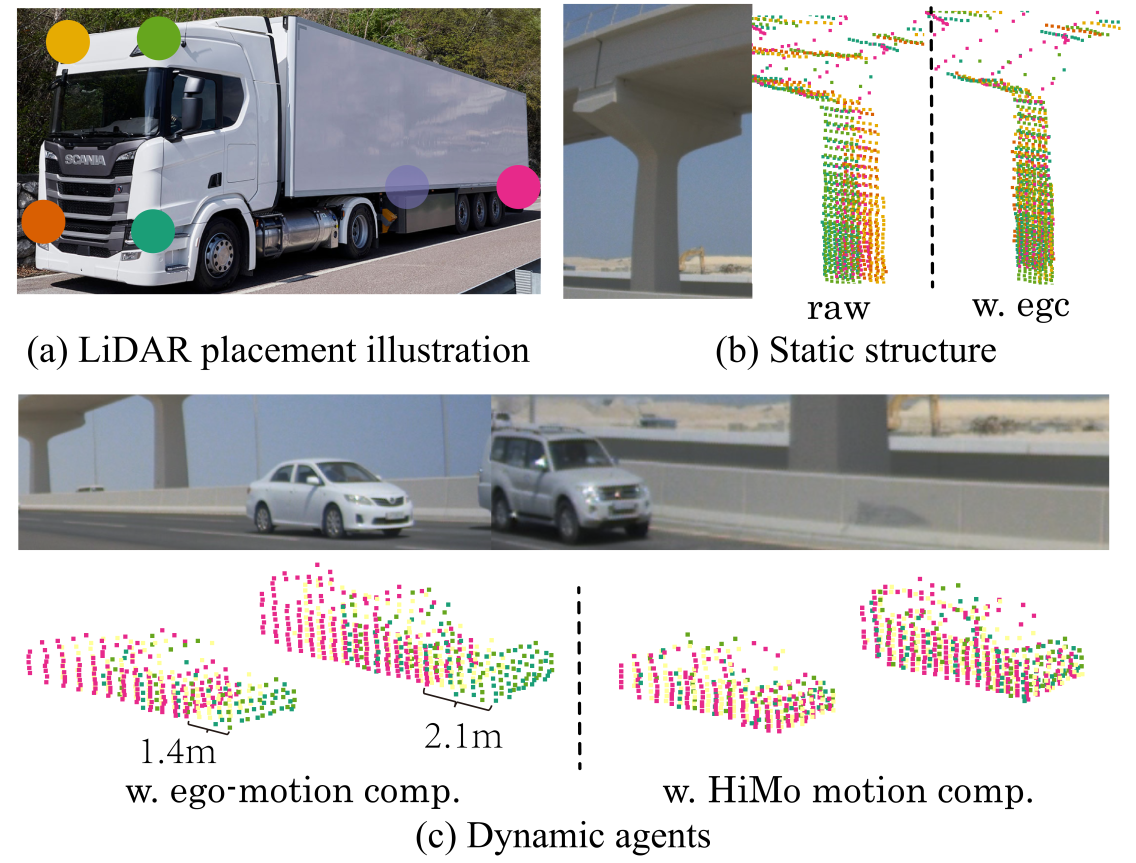
Figure 1: Multi-LiDARs are equipped in our heavy vehicles to avoid self-occlusion. (a) shows an example placement with 6 LiDARs. The point colors in (b-c) correspond to the LiDAR from which the points are captured. (b) illustrates the distortion of static structure due to fast-moving ego vehicle. Raw shows the raw data, w. egc shows the ego-motion compensation results. (c) demonstrates distortion caused by motion of other objects, which depends on the velocity of the said objects. In such case, ego-motion compensation alone (w. ego-motion comp.) is insufficient. In comparison, our HiMu pipeline (w. HiMo motion comp.) successfully undistorts the point clouds completely, resulting in an accurate representation of the objects.

There are two primary causes for LiDAR rolling shutter distortion: the motion of the ego vehicle and the motion of other agents in the scene. In the first case, the movement of the ego-vehicle, combined with the latency caused by the mechanical rotation of the LiDAR, leads to distorted representations of static objects or scenes. Such ego-motion induced distortion is well-studied in robotics [6]. In practice, localization algorithms [7, 8] and additional global positioning devices can be employed to accurately correct this distortion (see Fig. 1 (b)).

The second source of error – motion of other agents, on the other hand, is underexplored. In this scenario, the motion distortion is object-specific and depends on the relative velocity between the dynamic objects and the ego-vehicle. An example of this is shown in Fig. 1 (c), where the point cloud representation of the gray car is more elongated compared to the white car due to the higher velocity. As is visible in Fig. 1, ego-motion compensation alone cannot effectively address the distortion caused by dynamic objects. As a result, when sweeps of multiple LiDARs are combined, multiple copies of the same objects may appear in the merged point cloud, leading to inaccurate object appearances that complicate downstream tasks.

However, to the best of our knowledge, the distortion caused by dynamic objects has not yet been reported in common public datasets. This is likely due to the low speeds of other objects in these datasets. Existing open datasets in autonomous driving, such as KITTI [9], Argoverse [10, 11], Waymo [12] and Nuscenes [13], focus on urban environments, where the speeds of most dynamic objects are lower than 40 $\mathrm{k}\mathrm{m}\mathrm{/}\mathrm{h}$ (around 11.1 $\mathrm{m}\mathrm{/}\mathrm{s}$), as shown in Fig. 2. At such low speed, the distortion exists but is less pronounced (see Section III-A for details). Nonetheless, such distortions cannot be ignored when bringing autonomous driving solutions to real-world scenarios with large and fast-moving vehicles.

Figure 2: Distribution of object speeds in different datasets. Only objects with speeds exceeding 2$\mathrm{m}\mathrm{/}\mathrm{s}$ are included in the plot. The orange line shows the median speed and the blue dashed lines indicate the $\pm 10\%$ spread.

In this paper, we focus on this point cloud distortion problem and propose High-speed object Motion compensation (HiMo), a pipeline for non-ego vehicle motion compensation in point clouds. An example of HiMo compensated results is shown in Fig. 1 (c). Our primary contributions are as follows:

• We provide an in-depth analysis of motion-induced distortions in autonomous driving datasets, and highlight that high-speed objects have larger distortions.

• We propose HiMo, the first pipeline for dynamic object motion compensation, which repurposes scene flow estimation to undistort point clouds.

• We collect the first heavy-vehicle highway multi-LiDAR driving dataset (Scania), with significantly higher average object speed than existing datasets (see Fig. 2). This dataset therefore better exposes the distortion induced by dynamic objects.

• We design two evaluation metrics and benchmark state-of-the-art scene flow methods using HiMo pipeline on Argoverse 2 and Scania.

• We additionally present an improved self-supervised scene flow estimator that does not require human annotations and outperforms competing methods.

Our evaluation data and all code will be made publicly available upon publication.

II Related work

II-A Motion Compensation

As mentioned previously, the motion-induced distortion can be decomposed into two components. The first occurs due to the motion of the ego vehicle. In robotics and in particular within the field of Simultaneous Localication and Mapping (SLAM), existing methods [7, 8] account for this through ego-motion compensation to a specific timestamp, typically chosen to be in the middle of the LiDAR scan, or in the middle of a scan window in case of multiple LiDARs. The ego vehicle is typically assumed to be moving at a piece-wise constant velocity, and the coordinate of each point is transformed according to the displacement between the point’s timestamp and motion compensation timestamp. This is the baseline motion compensation strategy used in all public autonomous driving datasets.

The second component of this distortion occurs due to the motion of other agents in the scene and has received little attention so far. Ego-motion induced distortion is influenced by the motion over the entire duration of the LiDAR sweep. On the other hand, non-ego motion distortion is limited to the fraction of the time it takes to scan that object. See Section III-A for a more in-depth analysis. To our knowledge, there is no existing literature on undistorting raw point cloud data to compensate for non-ego motion distortion. The recent preprint [14] mentions that the distortion from the rolling shutter effect causes bad object mesh reconstruction. They focus on combining multiple frames and output mesh level reconstruction results while we focus on the distortion that happened in the single frame at the point level. Additionally, they require tracking labels from ground truth or a tracking network trained on annotated data.

In summary, our work aims to employ established self-supervised scene flow methods alongside ego-motion compensation to compensate for all distortions in the raw data properly. As such, our method is general and agnostic to the downstream application.

II-B Scene Flow Estimation

Scene flow estimation is the task of describing a 3D motion field between temporally successive point clouds [15, 16, 17, 18, 18, 19]. Existing works applied to autonomous driving dataset categorized into supervised training [20, 21, 22, 23] and self-supervised flow estimation [24, 25, 26, 27, 28, 29]. Supervised networks mainly use a backbone from object detection making them intractable to train on large point clouds and connecting a flow decoder output afterward. FastFlow3D [20] uses a feedforward architecture based on PointPillars [30], an efficient lidar detector architecture, enabling efficient training and inference of flow in the real world. DeFlow [21] integrates GRU [31, 32] with iterative refinement in the decoder design for voxel-to-point feature extraction and boosts the performance of flow estimation. However, expensive labeling of ground truth flow limits the scalability of these supervised methods. To train models without labeled data or directly optimize on runtime, researchers propose a self-supervised pipeline for scene flow estimation [24, 26, 27, 28, 33]. Neural Scene Flow Prior (NSFP) [26] provides high-quality scene flow estimates by optimizing ReLU and MLP layers at test time to minimize the Chamfer distance and maintain cycle consistency. FastNSF [27] leverage the same optimization but speed up through computing the chamfer loss by distance transform [34]. ICP-Flow [28] uses Iterative Closest Point (ICP) in each cluster of two point clouds and trains a feedforward neural network for real-time inference. SeFlow [24] tried in a different way by integrating dynamic awareness mapping to design four novel self-supervised loss terms for training networks from large datasets.

In this paper, we first repurpose scene flow estimation to object motion compensation, analyze the results and limitations between different self-supervised flow methods, and finally propose a new scene flow method, SeFlow++, with an improved version of dynamic auto-labeling and symmetric loss calculation.

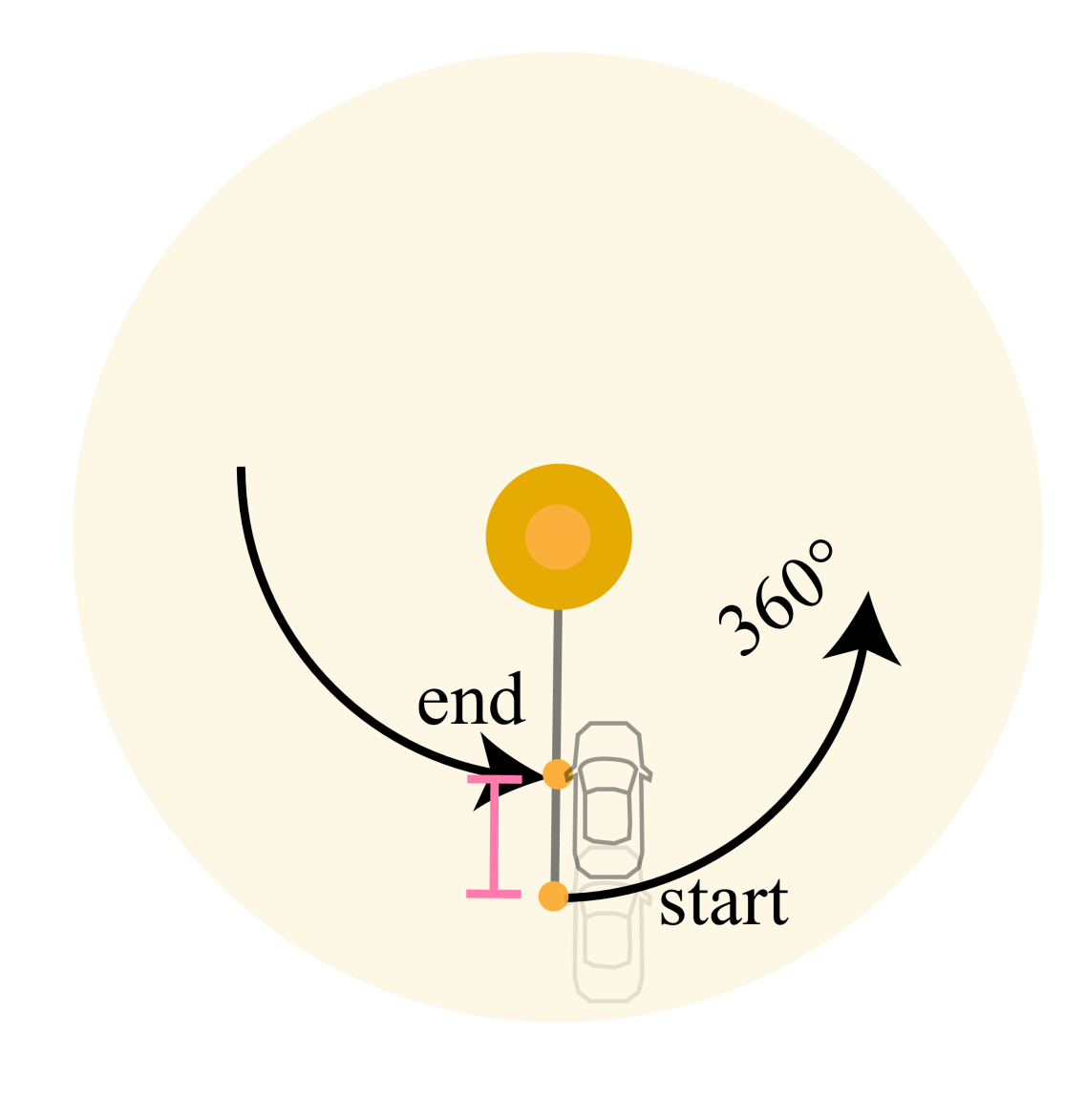
(a)

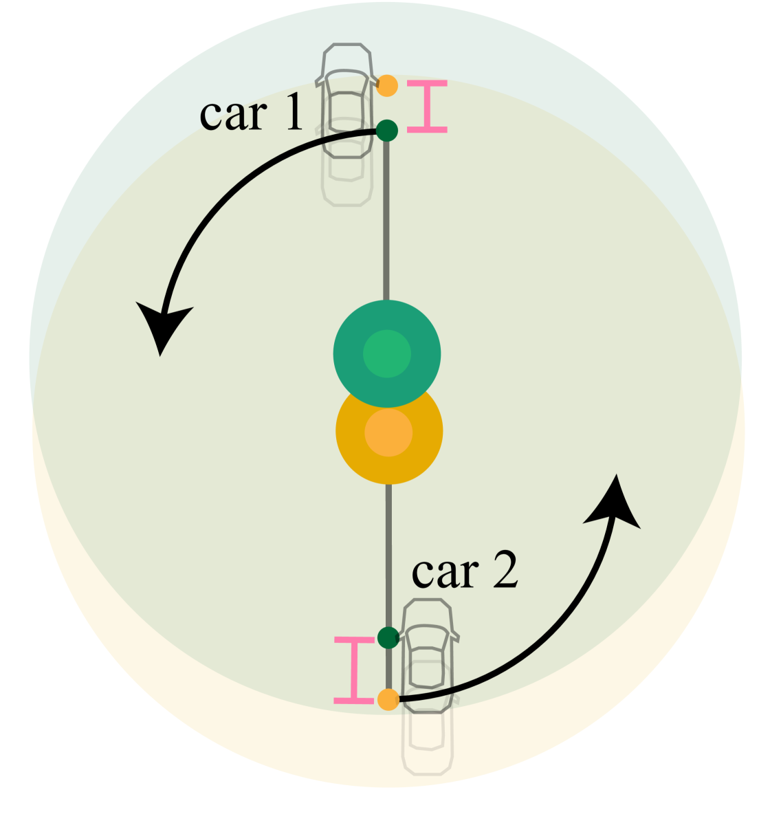
(b)

Figure 3: Top-view example of LiDAR sweeps showing how distortions are created for vehicles with (a) a single LiDAR and (b) two LiDARs. The small concentric circles of yellow and green are LiDARs. Both cases cause a displacement distance for the high-speed object. Light and dark cars show one car’s movement between two timestamps. (a) One complete single LiDAR scan sweep (small yellow dots are the first and last scan points). This case is only observed when moving objects are at the scan boundaries. (b) Two LiDAR scans separated in orientation by 180 degrees. This case is always observed for fast-moving objects.

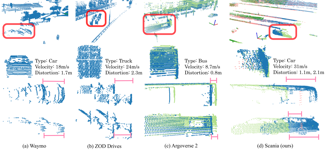
Figure 4: Examples of LiDAR distortion in various datasets. Ground points are removed in visualizations for a clearer view. Ego-motion compensation is applied [11, 12, 35]. In each column, the top images show the full scene, while the three images below show the front, top-down, and side views respectively. Different colors in (c) and (d) represent point clouds from separate LiDARs. The first two examples occur from a single LiDAR setup when an object is captured right at the beginning and the end of the scan (compare Fig. 3(a)). The latter two show the distortion in multiple LiDARs (compare Fig. 3(b)).

III Motion Compensation

In this section, we begin by discussing the point cloud distortion caused by dynamic objects in autonomous driving. We then propose our general HiMo pipeline to address this challenge.

III-A Rolling Shutter Distortion

Commonly used mechanical LiDAR sensors operate by sweeping laser beams in a horizontal ring pattern. This scanning process takes a certain amount of time to complete a full 360-degree sweep. If the sensed objects move during the scan, the captured point cloud will be distorted. The degree of the distortion is highly correlated with the velocity of the observed object ($v_{\text{object}}$) and sensor frequency ($f_{\text{sensor}}$), with the maximum distorted distance being $v_{\text{object}}/{f_{\text{sensor}}}$.

Fig. 3 illustrates this distortion in the single-LiDAR and multi-LiDAR scenarios. In the single-LiDAR case, this distortion is most visible when the dynamic object is positioned at the edge of the scan (see Fig. 3(a)). This can lead to severe shape distortion in the resulting point cloud. Fig. 4(a) and (b) provide examples from Waymo [36] and ZOD Drives [35], respectively.

In multi-LiDAR systems, the distortion problem is even more pronounced. As shown in Fig. 3(b), multiple LiDARs mounted on the same vehicle capture the same moving object at slightly different times and from different perspectives. This leads to multiple copies of the same object in the data. An example of this can be seen in Fig. 4(c) and (d) in Argoverse 2 [11] and our Scania dataset, respectively. In this figure, different colors represent point clouds from separate LiDARs combined into one observation frame within one scan interval. The distance between these differently colored copies of the object demonstrates the distortion effect in multi-LiDAR setups.

III-B HiMo Pipeline

In most public datasets, point cloud data is routinely ego-motion compensated [11, 36, 35]. However, as shown in Fig. 1 (c) and Fig. 4, this compensation cannot correct the distortions caused by the motion of other agents in the scene. To fully compensate for all dynamics in the scene, we propose the following HiMo pipeline.

Given the raw input point cloud from a scene $\mathcal{P}_{raw}$, the goal is to calculate a 3D undistorted vector for each point $\mathcal{D}(\mathbf{p})$. The estimated undistorted point cloud can be expressed as $\hat{\mathcal{P}}^{\prime}=\mathcal{P}_{raw}+\mathcal{D}$. A perfectly undistorted point cloud correctly describes the environment and removes all motion-related distortions.

In our work, the task of undistorting raw data is cast as a scene flow estimation problem. Note that the estimated 3D undistortion vector can be expressed as follows:

$$\hat{\mathcal{D}}(\mathbf{p})=\mathcal{V}(\mathbf{p})\Delta T(\mathbf{p}).$$ (1)

where $\Delta T(\mathbf{p})\in[0,T_{\text{sensor}}]$ is the time difference to the time of the most recent point in this LiDAR scan. The velocity of a point, $\mathcal{V}(\mathbf{p})$, can be approximated from its flow information by:

$$\mathcal{V}(\mathbf{p})=\hat{\mathcal{F}}(\mathbf{p})/T_{\text{sensor}},$$ (2)

where $T_{\text{sensor}}$ is the LiDAR scan interval ($T_{\text{sensor}}=1/f_{\text{sensor}}$). $\hat{\mathcal{F}}(\mathbf{p})=(x,y,z)^{T}$ is the output from the scene flow network and represents, for each point $\mathbf{p}$, the 3D flow from the current point cloud to the next.

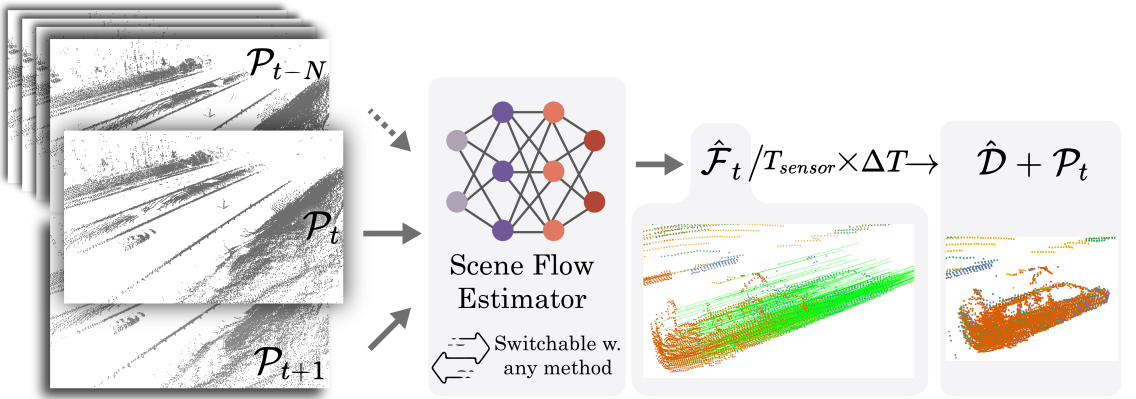
Figure 5: Schematic of the HiMo pipeline. This pipeline begins with the input of consecutive point clouds into a modular scene flow estimator. The estimator calculates the motion flow for each point in $\mathcal{P}_{t}$. This flow, along with known information on the elapsed time of each point and sensor frequency, is used to update point positions, resulting in a compensated point cloud that better represents high-speed moving objects.

In summary, the HiMo pipeline repurposes scene flow estimation for effective motion compensation. As shown in Fig. 5, the pipeline integrates multiple point clouds, sequentially processed by a scene flow estimator. Our pipeline can use any scene flow estimator, allowing for the adoption of improved scene flow methods as they emerge. By computing and applying scene flows, the pipeline effectively compensates for object movements, particularly enhancing the representation of high-speed objects.

IV Scene Flow

Scene flow is the core module in our HiMo motion compensation pipeline. To train or optimize a scene flow estimator, we need a supervision signal and a proper loss function. In supervised training, the signal is a human-labeled ground truth flow [21, 23]. However, human annotation for raw point clouds is costly and potentially prone to errors due to the distortions of high-speed vehicles. We therefore focus on self-supervised methods that do not rely on annotations. In the self-supervised field, runtime-optimization methods [26] need huge computational resources (10 to 30 GPU days) to undistort the large amounts of data. Knowledge distillation methods [24, 33, 28] spend time during training and are faster at runtime, which is important in practical applications when large amounts of data have to be undistorted. However, in our experiments, we found that they do not perform as well with little training data and for high-speed objects. To adapt to the high-speed regime and reduce the requirement on the amount of training data, we present a new scene flow method called SeFlow++, based on the previous state-of-the-art method SeFlow [24]. SeFlow++, presented in more detail below, uses an improved auto-labeler for supervision signal and symmetric self-supervised loss functions.

IV-A Auto-labeler

To achieve self-supervised training in scene flow, SeFlow [24] classify points into static and dynamic based on DUFOMap [37] and the dynamic points are clustered into object instances as shown in Fig. 6. This approach works well on point-level scene flow estimation. However, we observe that sometimes the error propagation from DUFOMap’s dynamic point classification to the subsequent clustering step results in misclassification of some static points as dynamic or vice versa.

Our refinement of the auto-labeling in SeFlow++ training is illustrated in Fig. 6. The auto-labeling process uses clustering and two dynamic classification methods on all points and reassigns dynamic labels based on these three sources.

Clustering: We cluster all points in $\mathcal{P}_{t}$ using HDBSCAN [38] into object instances $\mathcal{C}=\{c_{1},c_{2},\cdots,c_{n}\}$.

Dynamic classification: We use DUFOMap [37] and a threshold-based nearest neighbor method [39] to perform two independent dynamic classifications of all points in $\mathcal{P}_{t}$. The key insight of DUFOMap is that points observed inside a region that at one time has been observed as empty must be dynamic. The empty regions can be inferred via ray-casting from the sensor to point returns over past and future data. The result of DUFOMap for $\mathcal{P}_{t}$ is a dynamic point set $\mathcal{P}_{\text{dufo}}$.

For the threshold-based nearest neighbor method [39], the input is two consecutive point clouds $\mathcal{P}_{t},\mathcal{P}_{t+1}$. Its dynamic point set is defined as follows:

$$\mathcal{P}_{\text{nnd}}=\{\mathbf{p}|\mathrm{D}_{\text{min}}(\mathbf{p},\mathcal{P}_{t+1})>\mathrm{D}_{thres},\mathbf{p}\in\mathcal{P}_{t}\},$$ (3)

where $\mathrm{D}_{\text{min}}(\mathbf{p},\mathcal{P}_{t+1})$ represent the distance between point $\mathbf{p}$ and its nearest neighbor in $\mathcal{P}_{t+1}$.

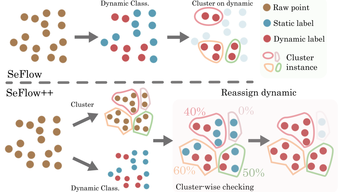
Figure 6: Dynamic auto-label process in SeFlow++ compared to SeFlow. Dynamic Class. means the dynamic classification procedure where SeFlow uses DUFOMap and SeFlow++ additionally uses another threshold nearest neighbor-based method. The Cluster-wise checking step in SeFlow++ reassigns labels based on whether the proportion of dynamic points labeled in cluster instances exceeds the thresholds.

Reassign label: Finally, the actual refinement is done at the cluster level with both $\mathcal{P}_{\text{nnd}}$ and $\mathcal{P}_{\text{dufo}}$. The subscript $t$ is ignored in the following equations to improve readability. More specifically, the subset of dynamic points are:

$$\mathcal{P}_{d}=\bigcup{\left\{\mathbf{p}|f(c),\mathbf{p}\in\mathcal{P}_{c},c\in\mathcal{C}\right\}},$$ (4)

where $\mathcal{C}$ is the set of all clusters based on HDBSCAN on $\mathcal{P}$, $c$ and $\mathbf{p}$ represent an individual cluster and a point in the cluster respectively. The function $f$ integrates the dynamics label from DUFOMap and threshold-based methods inside each cluster to refine the dynamic information. In our work, we define $f(c)$ as follows:

$$f(c)=\begin{cases}\tt{true},&\text{if }\min(r_{1},r_{2})\geq\tau_{1}~\&~\max(r_{1},r_{2})\geq\tau_{2}\\ \tt{false},&\text{otherwise}\end{cases}$$ (5)

where $r_{1}=\frac{|\mathcal{P}_{\text{dufo}}(c)|}{|\mathcal{P}_{c}|}$ and $r_{2}=\frac{|\mathcal{P}_{\text{nnd}}(c)|}{|\mathcal{P}_{c}|}$ represent the proportion of dynamic points labeled in cluster instance $c$ by the two methods respectively. $|\mathcal{P}|$ denotes the cardinality of (i.e., the number of points in) the point cloud $\mathcal{P}$. The decision thresholds $\tau_{1},\tau_{2}$ are hyperparameters to classify dynamic points. In all our experiments these were set to 5% and 10%, respectively. More specifically, for a cluster $c$ to be labeled as dynamic, the proportion of dynamic points in the cluster must exceed both thresholds simultaneously.

In summary, these steps provide our scene flow estimator with information about which points moved and to which cluster instance they belong roughly for afterward self-supervised training.

IV-B Self-supervised Loss

The most popular loss in self-supervised scene flow estimation is the Chamfer distance, a standard metric to measure the shape dissimilarity between two point clouds. The definition is:

$$\operatorname{CD}({\mathcal{P}}_{i},\mathcal{P}_{j})=\frac{\sum_{p\in{\mathcal{P}}_{i}}\mathrm{D}_{\min}(p,\mathcal{P}_{j})}{|{\mathcal{P}}_{i}|}+\frac{\sum_{p\in\mathcal{P}_{j}}\mathrm{D}_{\min}(p,\mathcal{P}_{i})}{|\mathcal{P}_{j}|}$$ (6)

In our previous work, SeFlow [24], we found that there are association errors in the Chamfer distance and proposed the following four-term loss function:

$$\mathcal{L}_{total}=\mathcal{L}_{\text{cham}}+\mathcal{L}_{\text{dcham}}+\mathcal{L}_{\text{static}}+\mathcal{L}_{\text{dcls}},$$ (7)

where $\mathcal{L}_{\text{cham}}$ and $\mathcal{L}_{\text{dcham}}$ are Chamfer distance loss on all points and only dynamic points respectively. $\mathcal{L}_{\text{static}}$ and $\mathcal{L}_{\text{dcls}}$ optimized flow estimation in static points and dynamic cluster instance points respectively.

Based on the above content, to better help self-supervise training, we propose a symmetric flow involving more supervision signals. Previously, [40] proposed a cycle consistency loss where the forward and backward flow between two point clouds are driven to match. Another example can be found in NSFP [26] that initializes two networks with the same architecture but with separate weights to optimize the forward and backward flows. However, switching input order or training two networks is not efficient especially when the number of points is large. Therefore, in our work, to maintain the same training efficiency and improve performance, we propose a symmetric flow loss calculation with a single forward pass. Due to symmetry around $\mathcal{P}_{t}$, applying the forward flow with a negative sign ($-$) effectively simulates a backward flow from $\mathcal{P}_{t}$ to $\mathcal{P}_{t-1}$. This insight allows the training step to compute both flow directions in a single forward pass, from $\mathcal{P}_{t}$ to $\mathcal{P}_{t+1}$, thereby streamlining the process.

We reformulate the first chamfer distance loss in Eq. 7 with symmetric flow calculation as follows:

$$\mathcal{L}_{\text{cham}}=\operatorname{CD}(\hat{\mathcal{P}}_{t+1},\mathcal{P}_{t+1})+\operatorname{CD}(\hat{\mathcal{P}}_{t-1},\mathcal{P}_{t-1}),$$ (8)

where $\hat{\mathcal{P}}_{t\pm 1}=\mathcal{P}_{t}\pm\hat{\mathcal{F}}_{t}$. We also apply dynamic chamfer distance $\mathcal{L}_{\text{dcham}}$ in the same way except it only considers points that are classified as dynamic in Eq. 4.

The last two loss terms in Eq. 7, the static loss and the dynamic cluster loss, are kept unchanged in this work. However, the dynamic point classification itself is refined as per description in Section IV-A. The static flow encourages the model to estimate zero flow for static points.

$$\mathcal{L}_{\text{static}}=\frac{1}{|{\mathcal{P}}_{s}|}\sum_{\mathbf{p}\in\mathcal{P}_{s}}||\Delta\hat{\mathcal{F}}(\mathbf{p})||_{2}^{2},$$ (9)

For the dynamic cluster loss, as in [24], we find the index of the point $p_{k}$ in cluster $c_{i}\in\mathcal{C}_{d}$ with the largest distance to its nearest neighbor point in $\mathcal{P}_{t+1,d}$, i.e.,

$$\kappa_{i}=\operatorname*{arg\,max}_{k}\{\mathrm{D}_{\min}(p_{k},\mathcal{P}_{t+1,d})|p_{k}\in\mathcal{P}_{c_{i}}\}.$$ (10)

We calculate the upper bound, $\tilde{f}_{c_{i}}$ on the flow for cluster $c_{i}$ as

$$\tilde{f}_{c_{i}}=p^{\prime}_{\kappa_{i}}-p_{\kappa_{i}},$$ (11)

where $p^{\prime}_{\kappa_{i}}$ is the nearest neighbor of point $p_{\kappa_{i}}$ in $\mathcal{P}_{t+1,d}$. We use this to drive the estimated flows of cluster $c_{i}$ towards $\tilde{f}_{c_{i}}$ as follows:

$$\mathcal{L}_{\text{dcls}}=\frac{1}{|\mathcal{P}_{t,d}|}{\sum_{c_{i}\in\mathcal{C}_{t,d}}\left(\sum_{p_{j}\in\mathcal{P}_{c_{i}}}||\hat{f}_{p_{j}}-\tilde{f}_{c_{i}}||^{2}_{2}\right)}.$$ (12)

V Experiments

In this section, we evaluate the proposed HiMo undistortion pipeline on our high-speed highway dataset as well as public autonomous driving datasets. We benchmark the motion compensation performance of HiMo with standard scene flow estimators and our proposed SeFlow++ estimator.

V-A Dataset

We evaluate our approach using two autonomous driving datasets: our (Scania) highway dataset and Argoverse 2 [11].

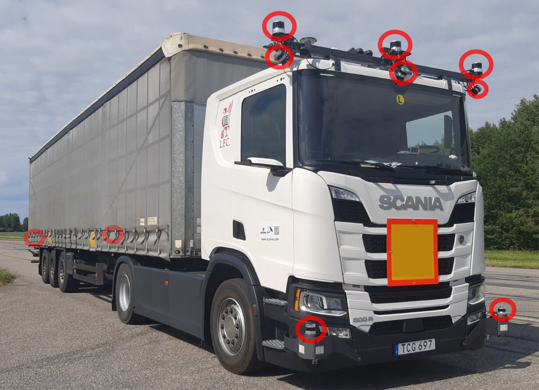
(a) Scania Truck

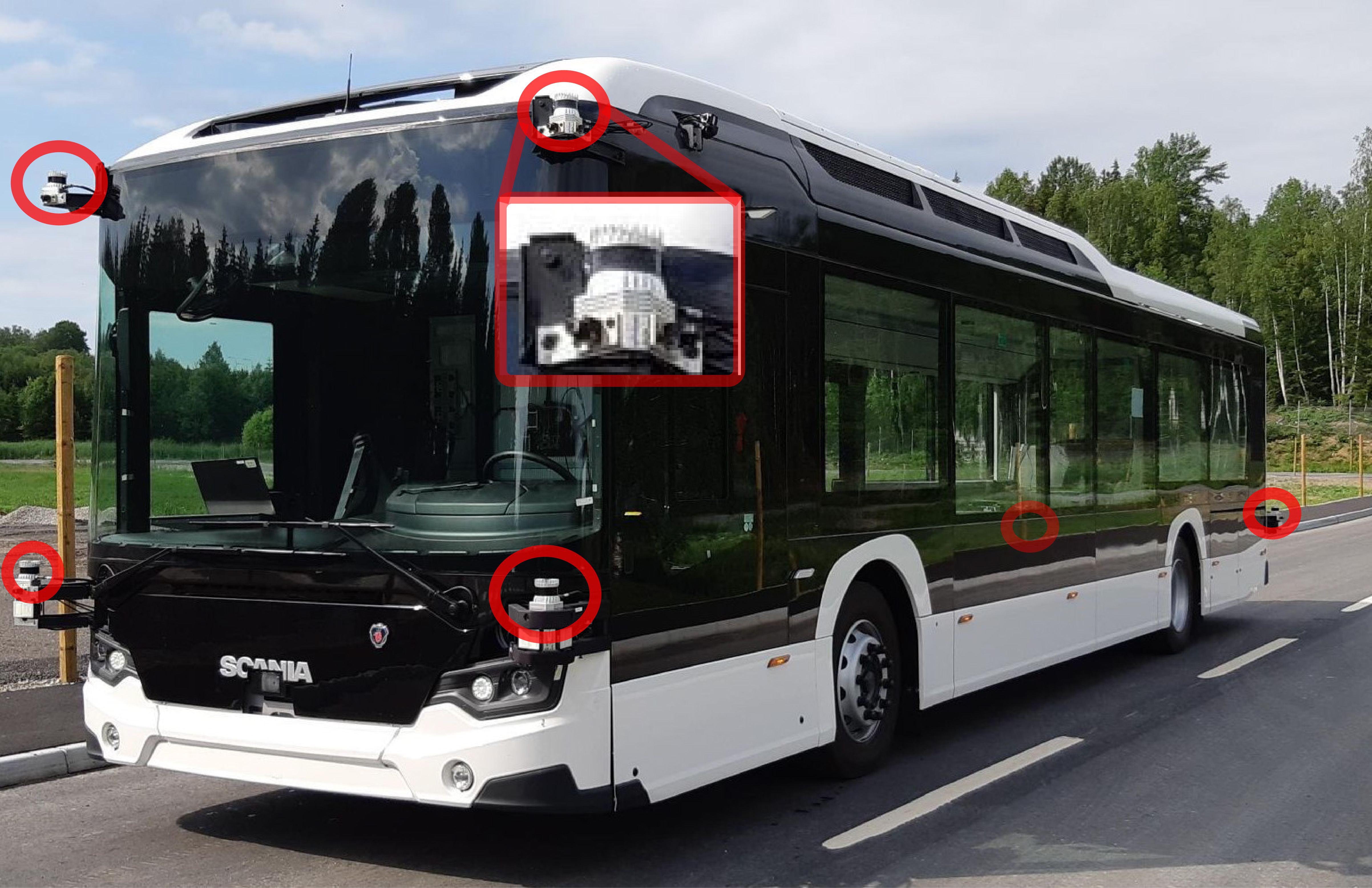
(b) Scania Bus

Figure 7: Two different setups for collecting our multi-LiDAR data are included in our evaluation data. (a) A truck with six LiDARs on the top of the truck and two on the front bottom. There are two at the back of the truck that are not visible in the image. (b) A bus with four in the front of the vehicle and two in the back of the bus.

TABLE I: Object motion compensation result comparisons using different scene flow methods in our HiMo pipeline on the Scania validation set. The first row reports the errors for raw data with ego-motion compensation only, and the rest also includes compensation for non ego-motion distortion using HiMo. Upper groups are supervised methods with scene flow networks trained on Argoverse 2 [11] and inference directly on the Scania dataset. Lower groups are self-supervised methods. $\pm$ means the standard deviation in the evaluation data (100 frames). All methods in the HiMo pipeline achieve better accuracy performance and object shape similarity compared to raw data. Our proposed SeFlow++ achieves state-of-art compensated performance in shape description for both car and other vehicle object types. The _↓blue value represents the error percentage decrease relative to the distorted raw data.

Methods		Reference	Chamfer Distance Error ↓			Mean Point Error ↓
			Total	CAR	OTHERS	Total	CAR	OTHERS
Ego-motion Compensation		-	0.284	0.257 $\pm$ 0.13	0.310 $\pm$ 0.11	0.935	0.913 $\pm$ 0.16	0.957 $\pm$ 0.07
HiMo (Ours)	FastFlow3D [20]	RAL2022	0.144 ↓49%	0.121 $\pm$ 0.04	0.168 $\pm$ 0.04	0.546 ↓42%	0.378 $\pm$ 0.16	0.714 $\pm$ 0.17
	DeFlow [21]	ICRA2024	0.088 ↓69%	0.057 $\pm$ 0.02	0.118 $\pm$ 0.05	0.315 ↓66%	0.139 $\pm$ 0.08	0.491 $\pm$ 0.19
	NSFP [26]	NeurIPS2021	0.073 ↓74%	0.064 $\pm$ 0.07	0.083 $\pm$ 0.04	0.255 ↓73%	0.188 $\pm$ 0.16	0.323 $\pm$ 0.15
	FastNSF [27]	ICCV2023	0.078 ↓72%	0.074 $\pm$ 0.05	0.081 $\pm$ 0.05	0.279 ↓70%	0.251 $\pm$ 0.16	0.308 $\pm$ 0.14
	ICP-Flow [28]	CVPR2024	0.183 ↓36%	0.203 $\pm$ 0.13	0.163 $\pm$ 0.05	0.695 ↓26%	0.698 $\pm$ 0.21	0.692 $\pm$ 0.18
	SeFlow [24]	ECCV2024	0.096 ↓66%	0.094 $\pm$ 0.04	0.098 $\pm$ 0.01	0.452 ↓52%	0.444 $\pm$ 0.17	0.461 $\pm$ 0.18
	SeFlow++ (Ours)	-	0.054 ↓81%	0.050 $\pm$ 0.03	0.059 $\pm$ 0.02	0.267 ↓72%	0.179 $\pm$ 0.10	0.356 $\pm$ 0.18

Our dataset consists of around 500 sequences, 10 to 15 seconds per sequence, captured in and around downtown Södertalje, Sweden. Our platforms, as shown in Fig. 7, consist of buses and trucks equipped with multiple LiDARs. The frequency of each LiDAR is around 10$\mathrm{H}\mathrm{z}$. Points from multiple LiDARs within a fixed time interval ($T_{sensor}$) are combined into a single point cloud.

Ground truth for evaluation: To evaluate the accuracy of the HiMo pipeline, we sent our evaluation data, which contains 100 frames from 20 different sequences, to a professional annotation institution to get 3D bounding box labels for every foreground object. Because of the distortion of the raw data, these ground truth bounding boxes are not consistent, especially for high-speed objects for which multiple copies are present in the raw data. To refine annotations, we follow [41] to optimize and estimate all bounding box velocities. The estimated velocities are used to enlarge the bounding boxes in their direction of motion to include all points (all ”copies” of the objects). For points inside these enlarged boxes, the estimated displacement is assigned as the ground truth for the scene flow for that object.

Argoverse 2 Sensor dataset encompasses 700 training and 150 validation scenes. They use a passenger car equipped with two roof-mounted VLP-32C lidar sensors. Each scene is approximately 15 seconds long in 10 Hz, with complete annotations for evaluation. However, the official ground truth bounding box is not fully correct on distorted objects, we inflate the length of each bounding box based on their annotated speed. To analyze the result in highspeed object motion compensation, the evaluation sequence is selected based on whether it includes at least three fast-moving annotated objects. Finally, we manually selected 20 sequences with a total of 100 frames to make sure they have correct ground truth compensation results for quantitative evaluation.

More interactive visualization results on Argoverse 2 [11] and ZOD Drive [35] are available on the project page.

V-B Evaluation Metrics

Due to the lack of well-established motion distortion metrics in the literature, we present two metrics: one captures shape similarity inspired by 3D reconstruction, and the other measures point-level accuracy similar to end point error in scene flow.

Shape similarity measures the correctness of shape descriptions. We use the chamfer distance to compute the similarity error between two instance point sets $c_{i}$ compensated by ground truth and estimated motion compensation,

$$\text{CDE}=\frac{1}{|\mathcal{C}_{gt}|}\sum_{c_{i}\in\mathcal{C}_{gt}}\left(\frac{|\mathcal{P}_{c_{i}}|}{|\mathcal{P}_{\mathcal{C}_{gt}}|}\times\text{CD}(\mathcal{P^{\prime}}_{est,c_{i}},\mathcal{P^{\prime}}_{gt,c_{i}})\right),$$ (13)

where $\mathcal{P^{\prime}}_{est,c_{i}}$ and $\mathcal{P^{\prime}}_{gt,c_{i}}$ denote the point set $c_{i}$ compensated using the estimated motion and ground truth, respectively. The smaller the chamfer distance, the greater the shape similarity between the estimated instance shape and the ground truth.

While we believe that shape similarity best measures a method’s ability to undistort moving objects, it is based on nearest neighbor matching that does not guarantee correct association at the point level. Therefore, we also look at the point-level accuracy that can be represented as the mean point error (MPE),

$$\text{MPE}=\frac{\sum_{c_{i}\in\mathcal{C}_{gt}}\left(\sum_{\mathbf{p}\in\mathcal{P}_{c_{i}}}\left\|\mathbf{p}_{est}-\mathbf{p}_{gt}\right\|_{2}\right)}{|\mathcal{C}_{gt}||\mathcal{P}_{\mathcal{C}_{gt}}|}$$ (14)

where $|\mathcal{P}_{c_{i}}|$, $|\mathcal{P}_{\mathcal{C}_{gt}}|$ denotes the cardinality of (i.e., the number of points in) the instance $i$ and all instances respectively and $|\mathcal{C}_{gt}|$ means the number of instances in the frame.

When using these two metrics, the CDE determines the performance, i.e., how well we undistorted the moving objects and MPE represents error at a point rather than a shape level. We separately report metrics for two different types of vehicles to better analyze the limitations. In all result tables, CAR means regular and passenger vehicles, and OTHER VEHICLES (OTHERS) include trucks, long buses, heavy vehicles, vehicles with trailers, etc.

V-C Evaluated Methods

In this work, we repurpose scene flow estimation to motion compensation with our HiMo pipeline. Given point cloud data as input, it outputs estimated distortion distances to undistort the point cloud as shown in Fig. 5. We compare our HiMo pipeline with the current best-practice baseline, i.e., doing only ego-motion estimation. The point cloud data in all datasets is already ego-motion compensated where the undistorted vector $\mathcal{D}$ is the velocity of the ego vehicle at current timestamp times with different $\Delta T(p)$ for each point. Below, we evaluate HiMo with different state-of-the-art scene flow estimators, including our new SeFlow++. The evaluated scene flow methods are outlined below.

1. FastFlow3D [20]: Supervised methods trained on Argoverse 2 sensor dataset. Pre-trained weights from [21].

2. DeFlow [21]: Supervised methods trained on Argoverse 2 sensor dataset. Pre-trained weights from [21].

3. NSFP [26]: A runtime optimization method that uses Chamfer distance between $\mathcal{P}_{t}+\hat{\mathcal{F}_{t}}$ and $\mathcal{P}_{t+1}$. It needs thousands of iterations to optimize a simple neural network to output the flow of each new frame frame.

4. FastNSF [27]: To speed up the runtime of NSFP, the paper proposes a distance transform to calculate the nearest neighbor error.

5. ICP-Flow [28]: This approach first processes point clouds with a clustering algorithm. Then it employs the conventional Iterative Closest Point (ICP) algorithm that aligns the clusters over time and outputs the corresponding rigid transformations.

6. SeFlow [24]: This method integrates efficient dynamic classification into a learning-based scene flow pipeline and designs three novel losses to achieve self-supervised flow training as described in Eq. 7.

7. SeFlow++ (Ours): Proposed in this paper, it is based on the insight of SeFlow with dynamic refinement labeling in Section IV-A and symmetric forward flow self-supervise loss supervision in Section IV-B.

TABLE II: Object motion compensation result comparisons using different scene flow methods in our HiMo pipeline on Argoverse 2. The first row reports the errors for raw data with ego-motion compensation only, and the rest also includes compensation for non ego-motion distortion using HiMo. Self-supervised methods are listed without human-labeled data needed to undistort raw data. $\pm$ means the standard deviation in the evaluation data (100 frames). All methods in the HiMo pipeline achieve better accuracy performance and object shape similarity compared to raw data. The _↓blue value represents the error percentage decrease relative to the distorted raw data.

Methods		Reference	Chamfer Distance Error ↓			Mean Point Error ↓
			Total	CAR	OTHERS	Total	CAR	OTHERS
Ego-motion Compensation		-	0.180	0.176 $\pm$ 0.02	0.185 $\pm$ 0.01	0.619	0.585 $\pm$ 0.13	0.654 $\pm$ 0.03
HiMo (Ours)	NSFP [26]	NeurIPS2021	0.052 ↓71%	0.073 $\pm$ 0.03	0.032 $\pm$ 0.01	0.144 ↓77%	0.209 $\pm$ 0.12	0.079 $\pm$ 0.02
	FastNSF [27]	ICCV2023	0.079 ↓56%	0.103 $\pm$ 0.03	0.054 $\pm$ 0.00	0.260 ↓58%	0.331 $\pm$ 0.14	0.190 $\pm$ 0.00
	ICP-Flow [28]	CVPR2024	0.053 ↓71%	0.060 $\pm$ 0.03	0.046 $\pm$ 0.00	0.135 ↓78%	0.168 $\pm$ 0.13	0.101 $\pm$ 0.00
	SeFlow [24]	ECCV2024	0.040 ↓78%	0.041 $\pm$ 0.01	0.039 $\pm$ 0.00	0.073 ↓88%	0.059 $\pm$ 0.02	0.088 $\pm$ 0.01
	SeFlow++ (Ours)		0.038 ↓79%	0.037 $\pm$ 0.01	0.040 $\pm$ 0.00	0.067 ↓89%	0.058 $\pm$ 0.02	0.077 $\pm$ 0.00

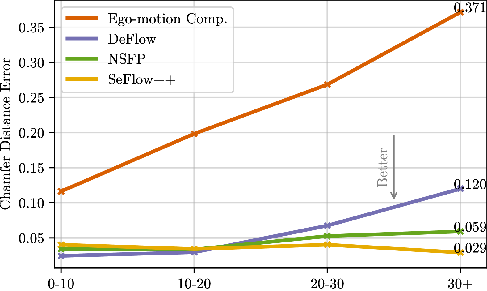
(a) Chamfer distance error v.s. object velocity ($\mathrm{m}\mathrm{/}\mathrm{s}$)

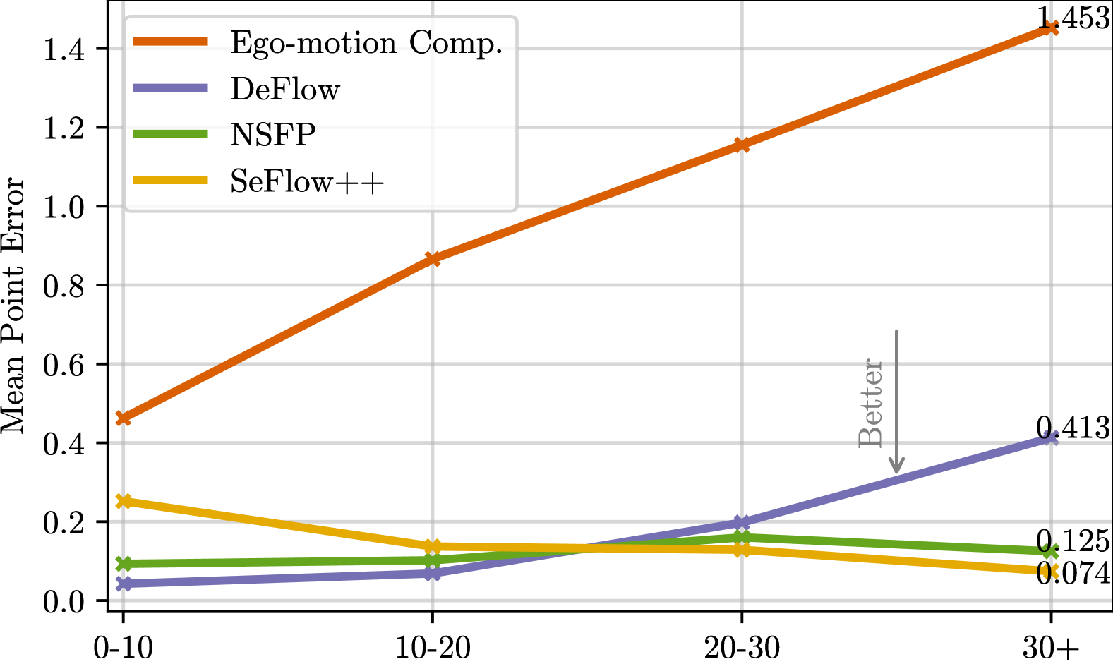
(b) Mean point error v.s. the object velocity ($\mathrm{m}\mathrm{/}\mathrm{s}$)

Figure 8: Error distribution concerning object velocity ($\mathrm{m}\mathrm{/}\mathrm{s}$) of CAR category for three best performing flow estimators in our HiMo pipeline on Scania data. The approximately linear relationship between velocity and error is clear in the ego-motion compensated data.

All code to reproduce results and run the HiMo pipeline can be found in https://github.com/KTH-RPL/HiMo. The main hyperparameters are listed here: learning rate ($2e^{-4}$) with Adam optimizer [42], batch size ($8$), the total training epoch ($9$). More configurations can be found in the code. All experiments are executed on a desktop powered by an Intel Core i9-12900KF CPU and equipped with a GeForce RTX 3090 GPU.

V-D Quantitative Results

The comparative analysis of different scene flow methods using the HiMo pipeline on the Scania dataset is detailed in Table I. The first row shows large CDE and MPE for the ego-motion only compensation baseline. Perfect undistortion would result in both metrics being zero. As shown in the rest of Table I, all scene flow methods used in the HiMo pipeline help reduce distortion errors. This demonstrates the effectiveness of our HiMo pipeline in motion compensation with up to 81% in shape improvement. However, when combined with different scene flow estimators, the performance of the HiMo pipeline differs. Despite not having seen Scania data before, DeFlow performs well on car-type objects according to both CDE and MPE. The reason behind this is that car-type objects in Argoverse 2 and Scania data are similar in shape. However, because of the other vehicle-type objects’ high-speed motion and long vehicle size, the raw distortion data cause difficulty in transferring the knowledge from the previous dataset. We can observe improved performance for the self-supervised methods, except ICP-Flow, on both point compensation accuracy and shape similarity (lower MPE and CDE on other vehicle categories compared to the supervised methods in Table I). The reason why ICP-Flow does not perform as well as others do is that ICP-Flow uses a lot of heuristics in its optimization and ICP; hence, one needs to tweak it for different data or scenarios. As shown in Table II, ICP-Flow performs much better on Argoverse 2 which it is optimized for. Our SeFlow++ scene flow method achieves the best performance with our HiMo pipeline in shape similarity after object motion compensation and yields comparable results on MPE.

The effectiveness of the HiMo pipeline is also demonstrated on other public datasets, such as Argoverse 2 as shown in Table II. The ego-motion compensated point cloud data from the selected high-speed scenarios in Argoverse 2 has lower CDE and MPE compared to our Scania data. This is caused by the lower object speeds. All self-supervised scene flow estimators in the HiMo pipeline can achieve at least a 50% error reduction.

Figure 9: Qualitative comparison of scene flow methods inside the HiMo pipeline for motion compensation on a distorted truck object. Top: Raw point cloud data with ego-motion compensation showing evident distortion. Bottom (left to right): Ground truth, SeFlow++ (Ours), SeFlow, and FastNSF results. Side and top views are provided for each method. CDE and MPE values are reported, demonstrating the visualization insight on point-level accuracy and shape preservation across different approaches.

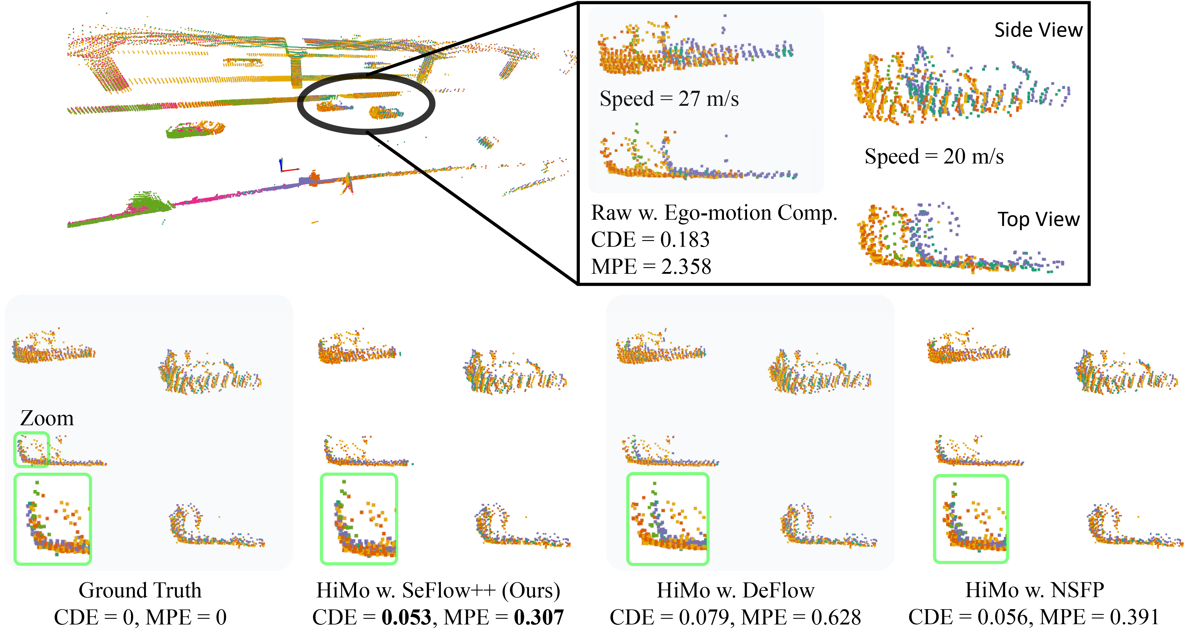
Figure 10: Qualitative comparison of scene flow methods inside the HiMo pipeline for motion compensation on two distorted regular car objects. Top: Raw point cloud data with ego-motion compensation showing evident distortion. Bottom (left to right): Ground truth, SeFlow++ (Ours), DeFlow, and NSFP results. Side and top views are provided for each method. All scene flow methods in the HiMo pipeline demonstrate effective compensation for the distorted data, with SeFlow++ showing superior performance in both metrics.

V-E Error Distribution

In Fig. 8, we explore the error distributions associated with car-type objects across varying velocities. The x-axis represents the velocity range of the objects, segmented into intervals (0-10 $\mathrm{m}\mathrm{/}\mathrm{s}$, 10-20 $\mathrm{m}\mathrm{/}\mathrm{s}$, etc.).

Looking at ego-motion compensated data reveals a direct correlation between the higher velocity of an object and the increase in error. This trend confirms our discussions on distortion impacts detailed in Section III-A.

Among the methods, DeFlow, which was trained on another dataset with ground truth supervision and directly applied to our Scania data, exhibits increased errors as the velocity of the object accelerates. This suggests that DeFlow’s adaptability to high-speed scenarios is constrained, likely due to its training not fully capturing the fast-moving dynamics. This pre-trained low performance on fast-moving objects reveals the necessity of self-supervised learning. NSFP and SeFlow++ (Ours) consistently have high accuracy and overall good performance underlining the advantages of self-supervised learning in managing rapid motion dynamics without significant error increases.

V-F Qualitative Results

Our qualitative analysis, as shown in Fig. 9, provides visual results into the performance of different motion compensation methods on a truck object that exhibits significant distortion. The data that is only ego-motion compensated demonstrates severe distortion effects on the truck, with its shape appearing extended and fragmented due to the motion during LiDAR scanning. All scene flow estimators in our HiMo pipeline, including SeFlow++ (Ours), SeFlow, and FastNSF, show improvements over only ego-motion compensation in terms of both quantitative metrics (CDE and MPE) and visual appearance. However, each method exhibits different aspects in its refinement results. SeFlow++ achieves the best visual similarity to the ground truth in terms of overall shape reconstruction. The truck’s outline and structure are more coherent and closely resemble the ground truth (Fig. 9.i), despite not having the best point accuracy. SeFlow demonstrates the best performance in terms of MPE, indicating high point-level accuracy. However, this superiority in point accuracy is not immediately apparent in the visual representation. Interestingly, SeFlow++ shows a more scattered point distribution at the center decomposition of the truck (Fig. 9.ii), which may result in its larger MPE despite better overall shape preservation. FastNSF provides a balanced performance, improving upon the raw data but not matching the refinement quality of SeFlow++ in terms of shape reconstruction or SeFlow in point accuracy. This observation highlights the importance of considering both shape similarity (CDE) and point-level accuracy (MPE) in evaluating motion compensation methods. While an ideal method would excel in both metrics, practical limitations often lead to tradeoffs. SeFlow++ demonstrates superior performance in preserving the overall shape of the truck, as evidenced by the lower CDE and visually coherent structure, despite not achieving the lowest MPE. This underscores the method’s strength in maintaining object integrity, which is crucial for downstream tasks in autonomous driving perception.

Another qualitative motion compensation result on two regular car objects is presented in Fig. 10. All methods in our HiMo demonstrate significant improvements in both metrics for cars, with more substantial reductions compared to the truck scenario. For instance, SeFlow++ achieves a remarkable 71% reduction in CDE and an 89% decrease in MPE. DeFlow, despite being trained on different datasets, shows competitive performance in CDE reduction (57% decrease to 0.079) for two CAR-type objects. However, its compensation for the faster-moving car (the left vehicle) with its speed standing 27 $\mathrm{m}\mathrm{/}\mathrm{s}$ appears less refined compared to SeFlow++ and NSFP, particularly in preserving the vehicle’s shape integrity.

The qualitative results in Fig. 9 and Fig. 10 of other flow methods in the HiMo pipeline can be found on the project page https://kin-zhang.github.io/HiMo. To show the generalization for our HiMo pipeline, Fig. 11 provides undistorted qualitative results in public datasets including Argoverse 2 [11] and ZOD Drives [35].

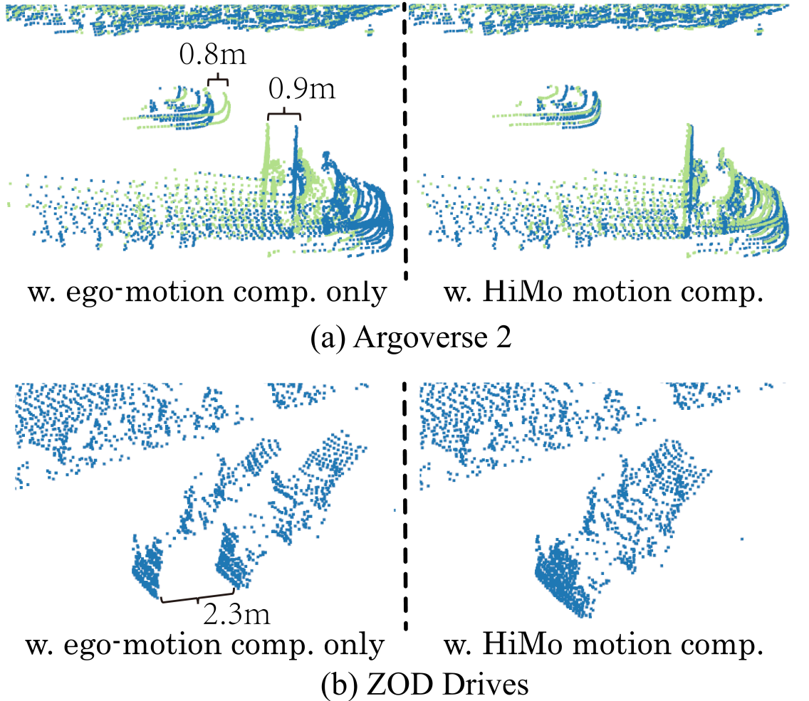
Figure 11: Our HiMo qualitative results on two public datasets with motion compensation in the data. Different point colors in Argoverse 2 represent different source lidar. The left half of the figure shows the ego-motion compensation results provided by the dataset, and the right side is our HiMo undistortion results.

V-G Computational Cost Comparison

In this section, we consider the computational cost for the three top-performing self-supervised methods in our HiMo pipeline: SeFlow++, NSFP, and FastNSF as shown in Table I. These methods differ significantly in training duration, inference time, and deployment efficiency, crucial factors for practical applications.

TABLE III: Comparative analysis of undistortion performance and total computational time. Performance is an average decreasing error percentage on CDE and MPE compared to raw data, illustrating the undistortion performance efficacy of each method in HiMo. Computational Time (hours) contains training time and undistortion inference time on the full Scania dataset (around 60,000 frames).

HiMo w. Flow Estimator	Performance ↑	Computational Time (h) Training + Inference    ↓
NSFP [26]	73.51%	0 + 250
FastNSF [27]	71.35%	0 + 83
ICP-Flow [28]	30.62%	0 + 150
SeFlow [24]	58.93%	12 + 0.8
SeFlow++ (Ours)	76.21%	14 + 1

As shown in Table III, SeFlow++ computational time can be decomposed to preparation time (auto-labeling) that is 4 hours, 10 GPU hours for training, and 1 hour inference time to undistort the whole raw dataset (around 60,000 frames). Despite this considerable initial investment before undistortion, the method excels in inference and deployment efficiency afterward in large datasets. It requires less than one GPU hour to perform motion compensation on the whole dataset (0.06 seconds per frame). Conversely, NSFP, the second top performance in our highway dataset on motion compensation, demands substantially more computational resources. It requires approximately 250 GPU hours to apply undistortion across all frames of the full dataset, averaging 15 seconds per frame. FastNSF, while quicker than NSFP, still necessitates about 83 GPU hours (three seconds per frame). Both methods, however, demonstrate considerable advantages in quick deployment when checking results in only a few frames. As they do not learn or store any weights but optimize afresh with every new input.

Nevertheless, given the increasing amount of data and the need for online undistortion in future scenarios, HiMo with SeFlow++ emerges as the more advantageous in terms of runtime. Its deployment speed is nearly 100 times faster than that of NSFP and 20 times faster than FastNSF.

VI Conclusion

In this paper, we addressed the critical issue of motion-induced distortions in LiDAR point clouds, which significantly impact the accuracy of environmental perception in autonomous driving systems. We analyzed the source of distortions and found that in addition to ego-motion, the motion of surrounding objects was a large source of distortion. Our investigation revealed the existence of moving object distortions across various datasets, particularly affecting high-speed objects and multi-LiDAR setups.

To tackle this challenge, we introduced HiMo, a novel pipeline that repurposes scene flow estimation for non-ego vehicle motion compensation. We also propose an improved self-supervised scene flow estimator SeFlow++ by refining the dynamic classification and adding a symmetric loss strategy. We demonstrated the effectiveness of HiMo through extensive experiments on our highway and public datasets. The results show that HiMo significantly improves the quality of point cloud representations. This enhancement not only potentially aids in more accurate object detection and tracking but also facilitates more consistent and precise data annotation, addressing a key challenge in multi-LiDAR setups. Our work contributes to the field by comprehensively analyzing point cloud distortions, proposing an effective compensation method, and offering open-source evaluation data and code.

Future work could explore the integration of HiMo with developing assistance 3D detection annotation systems as well as real-time perception systems.

Qingwen Zhang (Student Member, IEEE) received the M.Phil. degree from The Hong Kong University of Science and Technology in 2022. Her research interests in M.Phil. mainly include planning and imitation learning in autonomous driving. She is currently a Ph.D student at the KTH Royal Institute of Technology. Her research interests include dynamic awareness in point clouds.

Ajinkya Khoche (Student Member, IEEE) received the B.Tech., M.Tech. dual degree from Indian Institute of Technology Kharagpur in 2015, and M.Sc. degree from KTH Royal Institute of Technology Stockholm in 2020. He is currently an industrial Ph.D student at KTH Royal Institute of Technology and Scania. His research interests include multi-source fusion for long-range 3D perception.

Yi Yang (Student Member, IEEE) received the B.Sc degree from Shanghai Jiao Tong University in 2017. She completed her M.Sc. at KTH Royal Institute of Technology in 2019. She is currently an industrial PhD at KTH and Scania. Her research interests lie in autonomous driving, especially motion prediction, integrated with self-supervised learning and vision-language foundation models.

Li Ling (Student Member, IEEE) completed her M.Sc. in Machine Learning at KTH Royal Institute of Technology in 2021. She is currently a PhD student at KTH, funded by SMaRC (Swedish Maritime Robotics Center). Her research interests include 3D perception and bathymetry reconstruction using autonomous underwater vehicles.

Sina Sharif Mansouri obtained his Ph.D. degree from the Control Engineering Group in the Department of Computer Science, Electrical and Space Engineering at Luleå University of Technology. He was part of the CoSTAR team at Caltech during the DARPA Subterranean Challenge, where they won first place in the Urban Circuit. He also received Vattenfall’s award for the best doctoral thesis in 2021. He is currently the R&D Technical Leader for the Perception of Autonomous Vehicles at Scania.

Olov Andersson (Member, IEEE) is an Assistant Professor at KTH Royal Institute of Technology specializing in learning for autonomous systems. He received his PhD degree from Linköping University in 2020. Between 2020-2024 he was a postdoc and senior researcher in the Autonomous Systems Lab, ETH Zurich. In 2021 he won the DARPA SubT Challenge as part of team CERBERUS.

Patric Jensfelt (Member, IEEE) received his Ph.D. degree in Automatic Control in 2001 from the School of Electrical Engineering and since 2012 he is a professor of Computer Science at KTH Royal Institute of Technology. His research interests include system integration and perception for autonomous systems.

References

- [1] Y. Pan, X. Zhong, L. Wiesmann, T. Posewsky, J. Behley et al., “PIN-SLAM: Lidar slam using a point-based implicit neural representation for achieving global map consistency,” IEEE Transactions on Robotics (TRO), 2024.
- [2] X. Zhong, Y. Pan, J. Behley, and C. Stachniss, “Shine-mapping: Large-scale 3d mapping using sparse hierarchical implicit neural representations,” in Proceedings of the IEEE International Conference on Robotics and Automation (ICRA), 2023.
- [3] X. Zhong, Y. Pan, C. Stachniss, and J. Behley, “3D LiDAR Mapping in Dynamic Environments using a 4D Implicit Neural Representation,” in Proc. of the IEEE/CVF Conf. on Computer Vision and Pattern Recognition (CVPR), 2024.
- [4] M. Cao, S. Yang, Y. Yang, and Y. Zheng, “Rolling shutter correction with intermediate distortion flow estimation,” in Proceedings of the IEEE/CVF Conference on Computer Vision and Pattern Recognition (CVPR), 2024.
- [5] D. Qu, Y. Lao, Z. Wang, D. Wang, B. Zhao et al., “Towards nonlinear-motion-aware and occlusion-robust rolling shutter correction,” in Proceedings of the IEEE/CVF International Conference on Computer Vision (ICCV), October 2023, pp. 10 680–10 688.
- [6] I. MathWorks. (2024) Motion compensation in 3-d lidar point clouds using sensor fusion. [Online]. Available: https://se.mathworks.com/help/lidar/ug/motion-compensation-in-lidar-point-cloud.html
- [7] W. Xu, Y. Cai, D. He, J. Lin, and F. Zhang, “Fast-lio2: Fast direct lidar-inertial odometry,” IEEE Transactions on Robotics, vol. 38, no. 4, pp. 2053–2073, 2022.
- [8] T.-M. Nguyen, D. Duberg, P. Jensfelt, S. Yuan, and L. Xie, “Slict: Multi-input multi-scale surfel-based lidar-inertial continuous-time odometry and mapping,” IEEE Robotics and Automation Letters, vol. 8, no. 4, pp. 2102–2109, 2023.
- [9] A. Geiger, P. Lenz, C. Stiller, and R. Urtasun, “Vision meets robotics: The kitti dataset,” International Journal of Robotics Research (IJRR), 2013.
- [10] M.-F. Chang, J. W. Lambert, P. Sangkloy, J. Singh, S. Bak et al., “Argoverse: 3d tracking and forecasting with rich maps,” in Conference on Computer Vision and Pattern Recognition (CVPR), 2019.
- [11] B. Wilson, W. Qi, T. Agarwal, J. Lambert, J. Singh et al., “Argoverse 2: Next generation datasets for self-driving perception and forecasting,” in Proceedings of the Neural Information Processing Systems Track on Datasets and Benchmarks (NeurIPS Datasets and Benchmarks 2021), 2021.
- [12] P. Sun, H. Kretzschmar, X. Dotiwalla, and A. e. Chouard, “Scalability in perception for autonomous driving: Waymo open dataset,” in Proceedings of the IEEE/CVF Conference on Computer Vision and Pattern Recognition (CVPR), June 2020.
- [13] H. Caesar, V. Bankiti, A. H. Lang, S. Vora, V. E. Liong et al., “nuscenes: A multimodal dataset for autonomous driving,” in CVPR, 2020.
- [14] N. Chodosh, A. Madan, D. Ramanan, and S. Lucey, “Simultaneous map and object reconstruction,” 2024. [Online]. Available: https://arxiv.org/abs/2406.13896
- [15] S. Vedula, P. Rander, R. Collins, and T. Kanade, “Three-dimensional scene flow,” IEEE transactions on pattern analysis and machine intelligence, vol. 27, no. 3, pp. 475–480, 2005.
- [16] I. Khatri, K. Vedder, N. Peri, D. Ramanan, and J. Hays, “I can’t believe it’s not scene flow!” arXiv preprint arXiv:2403.04739, 2024.
- [17] C. Jiang, G. Wang, J. Liu, H. Wang, Z. Ma et al., “3dsflabelling: Boosting 3d scene flow estimation by pseudo auto-labelling,” in Proceedings of the IEEE/CVF Conference on Computer Vision and Pattern Recognition, 2024, pp. 15 173–15 183.
- [18] Y. Zhang, J. Edstedt, B. Wandt, P.-E. Forssén, M. Magnusson et al., “Gmsf: Global matching scene flow,” Advances in Neural Information Processing Systems, vol. 36, 2024.
- [19] J. Liu, G. Wang, W. Ye, C. Jiang, J. Han et al., “Difflow3d: Toward robust uncertainty-aware scene flow estimation with iterative diffusion-based refinement,” in Proceedings of the IEEE/CVF Conference on Computer Vision and Pattern Recognition, 2024, pp. 15 109–15 119.
- [20] P. Jund, C. Sweeney, N. Abdo, Z. Chen, and J. Shlens, “Scalable scene flow from point clouds in the real world,” IEEE Robotics and Automation Letters, vol. 7, no. 2, pp. 1589–1596, 2021.
- [21] Q. Zhang, Y. Yang, H. Fang, R. Geng, and P. Jensfelt, “DeFlow: Decoder of scene flow network in autonomous driving,” in 2024 IEEE International Conference on Robotics and Automation (ICRA), 2024, pp. 2105–2111.
- [22] A. Khoche, Q. Zhang, L. P. Sanchez, A. Asefaw, S. S. Mansouri et al., “Ssf: Sparse long-range scene flow for autonomous driving,” arXiv preprint arXiv:2501.17821, 2025.
- [23] J. Kim, J. Woo, U. Shin, J. Oh, and S. Im, “Flow4D: Leveraging 4d voxel network for lidar scene flow estimation,” IEEE Robotics and Automation Letters, pp. 1–8, 2025.
- [24] Q. Zhang, Y. Yang, P. Li, O. Andersson, and P. Jensfelt, “SeFlow: A self-supervised scene flow method in autonomous driving,” in European Conference on Computer Vision (ECCV). Springer, 2024, p. 353–369.
- [25] K. Vedder, N. Peri, I. Khatri, S. Li, E. Eaton et al., “Neural eulerian scene flow fields,” arXiv preprint arXiv:2410.02031, 2024.
- [26] X. Li, J. Kaesemodel Pontes, and S. Lucey, “Neural scene flow prior,” Advances in Neural Information Processing Systems, vol. 34, pp. 7838–7851, 2021.
- [27] X. Li, J. Zheng, F. Ferroni, J. K. Pontes, and S. Lucey, “Fast neural scene flow,” in Proceedings of the IEEE/CVF International Conference on Computer Vision, 2023, pp. 9878–9890.
- [28] Y. Lin and H. Caesar, “Icp-flow: Lidar scene flow estimation with icp,” arXiv preprint arXiv:2402.17351, 2024.
- [29] P. Vacek, D. Hurych, K. Zimmermann, and T. Svoboda, “Let-it-flow: Simultaneous optimization of 3d flow and object clustering,” IEEE Transactions on Intelligent Vehicles, pp. 1–10, 2024.
- [30] A. H. Lang, S. Vora, H. Caesar, L. Zhou, J. Yang et al., “Pointpillars: Fast encoders for object detection from point clouds,” in Proceedings of the IEEE/CVF conference on computer vision and pattern recognition, 2019, pp. 12 697–12 705.
- [31] K. Cho, B. Van Merriënboer, C. Gulcehre, D. Bahdanau, F. Bougares et al., “Learning phrase representations using rnn encoder-decoder for statistical machine translation,” arXiv preprint arXiv:1406.1078, 2014.
- [32] Y. Wei, Z. Wang, Y. Rao, J. Lu, and J. Zhou, “Pv-raft: Point-voxel correlation fields for scene flow estimation of point clouds,” in Proceedings of the IEEE/CVF conference on computer vision and pattern recognition, 2021, pp. 6954–6963.
- [33] K. Vedder, N. Peri, N. Chodosh, I. Khatri, E. Eaton et al., “ZeroFlow: Fast Zero Label Scene Flow via Distillation,” International Conference on Learning Representations (ICLR), 2024.
- [34] M. Asad, R. Dorent, and T. Vercauteren, “Fastgeodis: Fast generalised geodesic distance transform,” Journal of Open Source Software, vol. 7, no. 79, p. 4532, 2022. [Online]. Available: https://doi.org/10.21105/joss.04532
- [35] M. Alibeigi, W. Ljungbergh, A. Tonderski, G. Hess, A. Lilja et al., “Zenseact open dataset: A large-scale and diverse multimodal dataset for autonomous driving,” in Proceedings of the IEEE/CVF International Conference on Computer Vision, 2023.
- [36] P. Sun, H. Kretzschmar, X. Dotiwalla, A. Chouard, V. Patnaik et al., “Scalability in perception for autonomous driving: Waymo open dataset,” in Proceedings of the IEEE/CVF Conference on Computer Vision and Pattern Recognition (CVPR), June 2020.
- [37] D. Duberg, Q. Zhang, M. Jia, and P. Jensfelt, “DUFOMap: Efficient dynamic awareness mapping,” IEEE Robotics and Automation Letters, vol. 9, no. 6, pp. 5038–5045, 2024.
- [38] R. J. Campello, D. Moulavi, and J. Sander, “Density-based clustering based on hierarchical density estimates,” in Pacific-Asia conference on knowledge discovery and data mining. Springer, 2013, pp. 160–172.
- [39] M. Najibi, J. Ji, Y. Zhou, C. R. Qi, X. Yan et al., “Motion inspired unsupervised perception and prediction in autonomous driving,” in European Conference on Computer Vision. Springer, 2022, pp. 424–443.
- [40] H. Mittal, B. Okorn, and D. Held, “Just go with the flow: Self-supervised scene flow estimation,” in Proceedings of the IEEE/CVF conference on computer vision and pattern recognition, 2020, pp. 11 177–11 185.
- [41] A. Khoche, A. Asefaw, A. Gonzalez, B. Timus, S. S. Mansouri et al., “Addressing data annotation challenges in multiple sensors: A solution for scania collected datasets,” arXiv preprint arXiv:2403.18649, 2024.
- [42] D. Kingma and J. Ba, “Adam: A method for stochastic optimization,” in International Conference on Learning Representations (ICLR), San Diega, CA, USA, 2015.