Quantitative relaxation dynamics from generic initial configurations in the inertial Kuramoto model

Abstract.

We study the relaxation dynamics of the inertial Kuramoto model toward a phase-locked state from a generic initial phase configuration. For this, we propose a sufficient framework in terms of initial data and system parameters for asymptotic phase-locking. It can be roughly stated as set of conditions such as a positive initial order parameter, a coupling strength sufficiently larger than initial frequency diameter and intrinsic frequency diameter, but less than the inverse of inertia. Under the proposed framework, generic initial configuration undergoes three dynamic stages (initial layer, condensation and relaxation stages) before it reaches a phase-locked state asymptotically. The first stage is the initial layer stage in analogy with fluid mechanics, during which the effect of the initial natural frequency distribution is dominant, compared to that of the sinusoidal coupling between oscillators. The second stage is the condensation stage, during which the order parameter increases, and at the end of which a majority cluster is contained in a sufficiently small arc. Finally, the third stage is the persistence and relaxation stage, during which the majority cluster remains stable (persistence) and the total configuration relaxes toward a phase-locked state asymptotically (relaxation). The intricate proof involves with several key tools such as the quasi-monotonicity of the order parameter (for the condensation stage), a nonlinear Grönwall inequality on the diameter of the majority cluster (for the persistence stage), and a variant of the classical Łojasiewicz gradient theorem (for the relaxation stage).

1. Introduction

Synchronization refers to an adjustment of rhythms in interacting oscillatory systems, and it can be regarded as the formation of consensus in phases and frequencies among oscillators. The gradual appearance of synchronization from a desynchronized state is referred to as an emergent behaviror, and this is often observed in natural systems. To name a few, swarming of fish, flocking of birds, or aggregation of bacteria [4, 12, 68, 76, 80] etc. Despite its ubiquitous appearance in nature, synchronization was mathematically formulated only half a century ago by two pioneers Arthur Winfree [82, 83] and Yoshiki Kuramoto [54, 55]. They proposed mathematically tractable phase models that describe the dynamics of weakly interacting limit-cycle oscillators, and identified fundamental synchronous behavior.

The novel feature of Winfree and Kuramoto models is that they both exhibit phase transition phenomena from disordered states (incoherent states) to partially ordered states(partially phase-locked states) and then to fully ordered states (completely phase-locked states), as the coupling strength, a variable representing the amount of interaction between the individuals, exceeds certain critical threshold [5, 28, 56]. Due to this phase transition like feature, Winfree and Kuramoto’s mathematical approach to synchronous phenomena, and more generally the theory of weakly coupled oscillators, has received lots of attention from control theory, neuroscience, and statistical physics communities [1, 8, 9, 34, 39, 45, 50, 69, 71].

In this article, we are mainly interested in the inertial Kuramoto model which corresponds to the second-order correction of the Kuramoto model introduced by Arthur Bergen and David Hill [7] to model electric networks with generators, and by Bard Ermentrout [38] to model synchronous flashing of the firefly species Pteroptyx malaccae. Due to its second-order nature, the inertial Kuramoto model possesses several novel features absent in the Kuramoto model such as first-order phase transition [73] and hysteresis [49, 74].

To set up the stage, we begin with a brief description of the inertial Kuramoto model. Fix a positive integer $N$, the number of particles, and for $i\in[N]\coloneqq\{1,\cdots,N\}$, let $\theta_{i}=\theta_{i}(t)\in\mathbb{R}$ and $\omega_{i}={\dot{\theta}}_{i}$ be the phase and (instantaneous) frequency of the $i$-th Kuramoto oscillator, given as a real-valued function of nonnegative time $t\geq 0$. The dynamics of the phase ensemble $\{\theta_{i}\}_{i=1}^{N}$ under the inertial Kuramoto model is governed by the following Cauchy problem:

(1.1) $$\begin{cases}\displaystyle m\ddot{\theta}_{i}+\dot{\theta}_{i}=\nu_{i}+\frac{\kappa}{N}\sum_{j=1}^{N}\sin(\theta_{j}-\theta_{i}),\quad t>0,\\ \displaystyle(\theta_{i},{\dot{\theta}}_{i})\Big{|}_{t=0+}=(\theta_{i}^{0},\omega_{i}^{0}),\quad i\in[N].\end{cases}$$

Here, $m,\kappa$ and $\nu_{i}$ are nonnegative constants representing (positive uniform) inertia, coupling strength and natural (intrinsic) frequency of the $i$-th oscillators, respectively.

By the standard Cauchy-Lipschitz theory, the Cauchy problem (1.1) admits a global unique solution, which must be real analytic in terms of time and all other parameters by the Cauchy–Kovalevskaya theorem. Thus, in this paper, neither uniqueness, global existence, nor smoothness of solutions to (1.1) will be an issue. In what follows, we discuss main results of this paper.

1.1. Main results

The first set of results is concerned with the emergence of complete and partial phase-lockings. Roughly, it says that if initial configuration and system parameters satisfy

(1.2) $$\begin{aligned} &R(t)\coloneqq\left|\frac{1}{N}\sum_{j=1}^{N}e^{\mathrm{i}\theta_{j}(t)}\right|,\quad R(0)=R^{0}>0,\\ &\max\Bigg{\{}\frac{\displaystyle\max_{1\leq i,j\leq N}|\nu_{i}-\nu_{j}|}{\kappa},~~\frac{\displaystyle\max_{1\leq i,j\leq N}|\omega_{i}^{0}-\omega_{j}^{0}|}{\kappa},~~m\kappa\Bigg{\}}\ll|R^{0}|^{2},\end{aligned}$$

then the solution to (1.1) converges to a single traveling solution (see Theorem 1.1 below). Here, the symbol $\ll$ simply means the left-hand side is very smaller than the right-hand side in a non-rigorous manner. It will only be used when discussing heuristics; we do not assign a precise meaning.

Theorem 1.1.

Suppose the initial data and system parameters satisfy

(1.3) $$\frac{\displaystyle\max_{1\leq i,j\leq N}|\nu_{i}-\nu_{j}|}{\kappa}\leq x|R^{0}|^{2},\quad m\kappa\leq y|R^{0}|^{2},\quad\mathrm{and}\quad\frac{\displaystyle\max_{1\leq i,j\leq N}|\omega_{i}^{0}-\omega_{j}^{0}|}{\kappa}\leq z|R^{0}|^{2},$$

where $x,y,z$ are positive real numbers satisfying

(1.4) $$\begin{aligned} \inf_{\eta>0}&\Bigg{(}(1-e^{-\eta})y\left(\frac{1}{2}(z+\eta x)+(1-e^{-\eta})^{2}y(\frac{3}{4}z+\eta x+2\eta)\right)\\ &+\sqrt{3.068\left(y(x+2)+\max\{1,\eta\}e^{-\max\{1,\eta\}}yz+\frac{x}{2}+\frac{e^{-\eta}}{1-e^{-\eta}}\frac{z}{2}\right)}<1.\end{aligned}$$

Then, the following assertions hold.

1. (Asymptotic phase-locking): The global solution $(\Theta,\Omega:={\dot{\Theta}})$ (with $\Theta=(\theta_{1},\ldots,\theta_{N})$) to the Cauchy problem (1.1) exhibits “asymptotic phase-locking”:

   $$\exists\lim_{t\to\infty}(\theta_{i}(t)-\nu_{c}t),\quad\mathrm{and}\quad\lim_{t\to\infty}\dot{\theta}_{i}(t)=\nu_{c}\quad\mathrm{for~all~}i\in[N],$$

   where $\nu_{c}=\frac{1}{N}\sum_{i=1}^{N}\nu_{i}$ is the average of natural frequencies.

2. (Asymptotic partial phase-locking): There exists a subset $\mathcal{A}\subset[N]$ with $|\mathcal{A}|>\frac{N}{2}$ and integers $k_{i}$ for each $i\in\mathcal{A}$ such that

   $$\limsup_{t\to\infty}\max_{i,j\in\mathcal{A}}\Big{|}(\theta_{i}(t)-2k_{i}\pi)-(\theta_{j}(t)-2k_{j}\pi)\Big{|}<\frac{\pi}{2}$$

   and a constant $c=c(x,y,z,R^{0})$ such that for any $i,j\in\mathcal{A}$ with $\nu_{i}\geq\nu_{j}$,

   $$\frac{\nu_{i}-\nu_{j}}{\kappa}\leq\lim_{t\to\infty}(\theta_{i}(t)-\theta_{j}(t))\leq c\frac{\nu_{i}-\nu_{j}}{\kappa}.$$

Proof.

We will prove Theorem 1.1 assuming Theorem 4.1 in Appendix C. ∎

Remark 1.1.

Condition (1.4) is satisfied, for example, by

$$(x,y,z,\eta)=(0.5,0.015,0.12,1),(0.3,0.05,0.76,3).$$

These constants are artifacts of our proof and we do not claim that they are optimal, and Theorem 1.1 will follow from a more general framework, namely Theorem 4.1.

In literature [22, 23, 24, 25, 33, 32, 51, 81], the complete synchronization problem (or asymptotic phase-locking) has been investigated for the inertial Kuramoto model (1.1) for a restricted initial configuration. Numerical simulations suggest that the inertial Kuramoto model exhibits asymptotic phase-locking (as defined in the statement of Theorem 1.1 (1)) for generic initial data in the large coupling regime. Thus, we are led to ask the following question.

Question 1.1.

(Existence of critical coupling strength)  For a fixed natural frequency vector ${\mathcal{V}}=(\nu_{1},\ldots,\nu_{N})$ and Lebesgue a.e. initial data $(\Theta^{0},\Omega^{0})$ (with $\Theta^{0}=(\theta_{1}^{0},\ldots,\theta_{N}^{0})$ and $\Omega^{0}=(\omega_{1}^{0},\ldots,\omega_{N}^{0})$), does there exist a critical value $\kappa_{c}=\kappa_{c}({\mathcal{V}},\Theta^{0},\Omega^{0})$ such that $\kappa>\kappa_{c}$ implies asymptotic phase-locking in system (1.1), regardless of the inertia $m>0$?

From this point of view, the contribution of Theorem 1.1 is that it guarantees a range $\kappa\in[\kappa_{1},\kappa_{2}]$, where $\kappa_{1}$ is a function of ${\mathcal{V}},~\Theta^{0},~\Omega^{0}$ and $\kappa_{2}={\mathcal{O}}(|R^{0}|^{2}/m)$, at which asymptotic phase-locking occurs. To our knowledge, Theorem 1.1 is the first in the literature to provide a sufficient framework for asymptotic phase-locking for the inertial Kuramoto model (1.1) in the generality of generic initial data.

As for the physical significance of the second-order model (1.1), Ermentrout [38] considered (1.1) as a model for frequency modulation, essentially writing the ODE of (1.1) as

$$\ddot{\theta}_{i}=\frac{1}{m}(\nu_{i}-\dot{\theta}_{i})+\frac{\kappa}{mN}\sum_{j=1}^{N}\sin(\theta_{j}-\theta_{i}).$$

Note that the right-hand side can be regarded as competition between two forcing terms. More precisely, the term $\frac{1}{m}(\nu_{i}-\dot{\theta}_{i})$ denotes the tendency of the frequency to return to the natural frequency $\nu_{i}$, whereas the term $\frac{\kappa}{mN}\sin(\theta_{j}-\theta_{i})$ represents the enforcing consensus via the phase response of the $i$-th oscillator to the $j$-th oscillator.

Bergen and Hill [7] considered the Cauchy problem (1.1) as the swing dynamics for a power network consisting of $N$ electrical generators [14, 53, 70]: the inertial term $m\ddot{\theta}_{i}$ corresponds to the generator inertia; the dissipative terms $\dot{\theta}_{i}$ correspond to the loads or the mechanical damping; the intrinsic frequencies $\nu_{i}$ correspond to power injections; the nonlinear interaction terms $\frac{\kappa}{N}\sin(\theta_{j}-\theta_{i})$ correspond to the power flows along transmission lines; and synchronization is interpreted as robustness or transient stability [30, 31, 33, 34, 41, 42, 72]. From this point of view, the inertial Kuramoto model has found an application as an elementary model for “smart grids” [35]. The case $m=0$, i.e., the model (2.1), signifies that the nodes have loads and no generation. One could also consider systems with pure generation and zero load or damping [46] as well.

There has been recent interest in low-inertia power grids [63]: conventional fossil fuel-based power plants, which often involve steam and hydroelectric turbines, tend to have high inertia, whereas renewable energy sources such as solar and wind energy tend to have low inertia. How does one understand the stability and synchronization properties of such low-inertia power grids? In this light, the present work develops a theory of synchronization applicable in the low-inertia setting.

As by-products of the arguments employed in the proof of Theorem 1.1, we can obtain improved results for specific situations. First, we obtain a condition for partial phase-locking (see Definition 2.2), which states that if a majority of the oscillators is contained in a sufficiently small arc, it becomes self-sustaining and limits the dynamics of other oscillators. See Theorem 5.1. A cruder version of this idea has already appeared in [51]; their results are subsumed under Theorem 5.1. Second, we provide a framework more general than that of Theorem 1.1, namely Theorem 4.1. Third, we deal with a complete phase-locking for a three-oscillator system for all initial data:

Theorem 1.2.

Suppose that system parameters satisfy

$$N=3,\quad m\max_{1\leq i,j\leq N}|\nu_{i}-\nu_{j}|+2m\kappa+\frac{\displaystyle\max_{1\leq i,j\leq N}|\nu_{i}-\nu_{j}|}{2\kappa}<\frac{1}{8}\sqrt{\frac{1}{6}(69-11\sqrt{33})}\approx 0.123003.$$

Then, the solution to (1.1) exhibits asymptotic phase-locking.

Proof.

We provide the proof in Appendix D, after proving the equivalence of asymptotic phase-locking and finiteness of collisions in the small inertia regime $m\kappa\leq\frac{1}{4}$. ∎

Besides Theorem 1.1 and Theorem 1.2, we have a plethora of new results in this paper, namely Theorem 3.1, Theorem 4.1, Theorem 5.1, Theorem D.1, Proposition 2.1, Proposition 3.1, Proposition 3.2, Proposition 3.3, Proposition 3.4, and Corollary 5.1.

1.2. Roadmap

The rest of this paper is organized as follows. Below, we summarize some notations and conventions to be used throughout the paper. In Section 2, we first recall the (first-order) Kuramoto model and related results on asymptotic phase-locking and then demonstrate Galilean invariance and the corresponding momentum conservation of (1.1) and (2.1). We use this to provide natural definitions of complete and partial phase-lockings. This sheds light on why we obtain single traveling solutions with group frequency $\nu_{c}$ in the conclusions of Theorem 1.1. We then pose our main questions on the emergence of phase-locking.

In Section 3, we explain our basic rationale behind analysis of (1.1), which is to approximate it to the Kuramoto model (2.1). This process requires the smallness of $\displaystyle\max_{1\leq i,j\leq N}|\omega_{i}^{0}-\omega_{j}^{0}|/\kappa$ and $m\kappa$.

In Section 4, we explore three synchronization mechanisms of models (1.1) and (2.1), namely stability of majority clusters (subsection 4.2), quasi-monotonicity of the order parameter (subsection 4.3), and inertial gradient flow formulation of (1.1) and resulting application of the Łojasiewicz gradient theorem (subsection 4.1). These mechanisms require, in addition, the smallness of $\displaystyle\max_{1\leq i,j\leq N}|\nu_{i}-\nu_{j}|/\kappa$. We conjecture that this third mechanism can be used to fully characterize the asymptotic behaviors of models (1.1) and (2.1).

In Section 5, we study the properties of the majority cluster to establish a sufficient criteria for partial phase-locking.

In Section 6, we use that the second-order model (1.1) converges to the first-order model (2.1) in the zero inertia limit $m\to 0+$ to obtain a qualitative version of the phase-locking theorem, namely Theorem 3.1.

In Section 7, we present detailed proofs for presented main results. Finally, Section 8 is devoted to a brief summary of the main results and discussions for future work. In appendix sections, we provide the various technical details alluded throughout the paper.

1.3. Notations and conventions

We fix some notations and conventions for the remainder of the paper. Let $(\theta_{1},\ldots,\theta_{N})$ be a solution to (1.1) or (2.1). We denote $\omega_{i}(t)\coloneqq\dot{\theta}_{i}(t)$. We use capital Greek letters to denote the collection of the corresponding lower Greek letters:

$$\Theta\coloneqq(\theta_{1},\ldots,\theta_{N}),\quad\Omega\coloneqq(\omega_{1},\ldots,\omega_{N}),\quad\mathcal{V}\coloneqq(\nu_{1},\ldots,\nu_{N}).$$

We will use $\omega_{i}$ and $\dot{\theta}_{i}$ interchangeably and $\Omega$ and $\dot{\Theta}$ interchangeably throughout this article. We denote ${\bf 1}_{[N]}=(1,\cdots,1)\in{\mathbb{R}}^{N}$. For vectors $X=(x_{i})^{N}_{i=1}\in\mathbb{R}^{N}$ and $Y=(y_{i})^{N}_{i=1}\in\mathbb{R}^{N}$, we denote their exterior product $X\wedge Y\in\bigwedge^{2}\mathbb{R}^{N}$. For the standard basis $e_{1},\cdots,e_{N}$ of $\mathbb{R}^{N}$, we consider $e_{i}\wedge e_{j}$, $i,j\in[N]$, $i<j$ to be the standard basis of $\bigwedge^{2}\mathbb{R}^{N}$. Thus, in these coordinates, we may write

$$X\wedge Y=(x_{i}y_{j}-x_{j}y_{i})_{i,j\in[N],i<j}.$$

As usual, we use $\|\cdot\|_{p}$ to denote the $\ell_{p}$-norm in $\mathbb{R}^{N}$:

$$\|\Theta\|_{p}\coloneqq\left(\sum_{i=1}^{N}|\theta_{i}|^{p}\right)^{\frac{1}{p}},~1\leq p<\infty,\quad\|\Theta\|_{\infty}\coloneqq\max_{1\leq i\leq N}|\theta_{i}|.$$

We use $\mathcal{D}$ to denote the diameter: for a vector $X=(x_{i})^{N}_{i=1}\in\mathbb{R}^{N}$,

$$\mathcal{D}(X)\coloneqq\max_{1\leq i,j\leq N}|x_{i}-x_{j}|.$$

For example, for the above configurations $\Theta,\Omega$ and ${\mathcal{V}}$, we denote

$$\begin{aligned} {\mathcal{D}}(\Theta)\coloneqq\max_{1\leq i,j\leq N}|\theta_{i}-\theta_{j}|,\quad{\mathcal{D}}(\Omega)\coloneqq\max_{1\leq i,j\leq N}|\omega_{i}-\omega_{j}|,\quad{\mathcal{D}}(\mathcal{V})\coloneqq\max_{1\leq i,j\leq N}|\nu_{i}-\nu_{j}|.\end{aligned}$$

For $X\in\mathbb{R}^{N}$, we have

$$\mathcal{D}(X)=\|X\wedge{\bf 1}_{[N]}\|_{\infty},$$

where we endow $\bigwedge^{2}\mathbb{R}^{N}$ the $\ell_{\infty}$ norm with respect to its standard basis. We observe the triangle inequality

(1.5) $$|\mathcal{D}(A)-\mathcal{D}(B)|\leq\mathcal{D}(A-B),\quad A,B\in\mathbb{R}^{N}.$$

We observe the inequality

$$\frac{1}{2}\mathcal{D}(X)\leq\|X\|_{\infty},\quad X\in\mathbb{R}^{N},$$

which follows from the identity

(1.6) $$\|X\|_{\infty}-\frac{1}{2}\mathcal{D}(X)=\frac{1}{2}\left|\max_{i\in[N]}x_{i}+\min_{i\in[N]}x_{i}\right|,\quad X=(x_{1},\cdots,x_{N})\in\mathbb{R}^{N}.$$

We also denote the variances as follows:

$$\begin{aligned} \operatorname{Var}(\mathcal{V})\coloneqq\frac{1}{N}\sum_{i=1}^{N}|\nu_{i}-\nu_{c}|^{2},\quad\operatorname{Var}(\Omega^{0})\coloneqq\frac{1}{N}\sum_{i=1}^{N}|\omega_{i}^{0}-\omega_{c}|^{2}.\end{aligned}$$

It is well known that

$$\operatorname{Var}(X)\leq\frac{\mathcal{D}(X)^{2}}{4},\quad X\in\mathbb{R}^{N}.$$

For $\mathcal{A}\subset[N]$ and $X=(x_{i})_{i=1}^{N}\in\mathbb{R}^{N}$, we define the restricted vector

$$X_{\mathcal{A}}\coloneqq(x_{i})_{i\in\mathcal{A}}\in\mathbb{R}^{|\mathcal{A}|}.$$

The concepts of $\mathcal{D}(X_{\mathcal{A}})$ and $\|X_{\mathcal{A}}\|_{p}$ are defined in the same manner:

$$\mathcal{D}(\Theta_{\mathcal{A}})\coloneqq\max_{i,j\in\mathcal{A}}|\theta_{i}-\theta_{j}|,\quad{\mathcal{D}}(\Omega_{\mathcal{A}})\coloneqq\max_{i,j\in\mathcal{A}}|\omega_{i}-\omega_{j}|,\quad{\mathcal{D}}(\mathcal{V}_{\mathcal{A}})\coloneqq\max_{i,j\in\mathcal{A}}|\nu_{i}-\nu_{j}|.$$

and

$$\|\Theta_{\mathcal{A}}\|_{p}\coloneqq\Big{(}\sum_{i\in\mathcal{A}}|\theta_{i}|^{p}\Big{)}^{\frac{1}{p}},~1\leq p<\infty,\quad\|\Theta_{\mathcal{A}}\|_{\infty}\coloneqq\max_{i\in\mathcal{A}}|\theta_{i}|.$$

Throughout the paper, we call $m$, $\kappa$, and $\mathcal{V}$ system parameters, $\Theta^{0}$ and $\Omega^{0}$ initial data, and all other external parameters free parameters. We sometimes say ‘parameters’ to refer to any of these variables.

Although (1.1) describes a dynamical system on $({\mathbb{S}}^{1})^{N}\times{\mathbb{R}}^{N}$, we will interpret it as a dynamical system on $\mathbb{R}^{N}\times{\mathbb{R}}^{N}$, to avoid the existence issue of the scalar potential $P$ defined in (4.1). However, we will still use the geometric concept of an arc, i.e., a connected component of ${\mathbb{S}}^{1}$, as this will help to visualize the configuration geometrically. Anytime this terminology is used, various statements must be understood modulo $2\pi$. For example, whenever we say some oscillators $\Theta_{\mathcal{A}}$ are contained in an arc of length $\ell$, we will express this with $\mathcal{D}(\Theta_{\mathcal{A}})\leq\ell$; when we say this it will be clear that we can make harmless $2\pi$-translations of $\Theta_{\mathcal{A}}$ that do not affect the conclusions of our theorems nor the logical structure of their proofs.

2. Preliminaries

In this section, we study several preparatory facts to be used in later sections. First, we briefly review the related result for the Kuramoto model on asymptotic phase-locking, and the translation invariance property of the inertial Kuramoto model, phase-locked states as relative equilibria and symmetries related to the inertial Kuramoto model.

2.1. The Kuramoto model

The (globally coupled) first-order Kuramoto model, originally proposed by Kuramoto in [54, 55], is the model formally obtained from (1.1) by taking zero inertia $m=0$ and unit damping coefficient:

(2.1) $$\begin{cases}\displaystyle\dot{\theta}_{i}=\nu_{i}+\frac{\kappa}{N}\sum_{j=1}^{N}\sin(\theta_{j}-\theta_{i}),\quad t>0,\\ \displaystyle\theta_{i}\Big{|}_{t=0+}=\theta_{i}^{0},\quad i\in[N].\end{cases}$$

Again, by the standard Cauchy-Lipschitz theory and Cauchy-Kovalevskaya theorem, the model (2.1) admits global unique analytic solutions.

There have been lots of studies [2, 10, 26, 21, 32, 34, 36, 37, 65, 44, 47, 52, 77] on the asymptotic dynamics of the models (2.1) and their variants. Indeed, the aforementioned references provide several sufficient frameworks for the complete synchronization problem in which all the relative frequencies tend to zero asymptotically in a large coupling regime, for initial data restricted in a half-circle when the intrinsic velocities $\nu_{i}$ are distinct, and for a generic initial configuration when the intrinsic velocities $\nu_{i}$ are identical. Similarly to (1.1), the complete synchronization problem seems to be numerically true for all generic data in a large coupling regime, even for nonidentical intrinsic velocities $\nu_{i}$ [32, 47]. However, to verify this simple fact is difficult.

In recent works [44, 47], the authors provided sufficient conditions for generic initial data and coupling strength leading to the complete synchronization via the gradient flow formulation of (2.1) and technical estimates on the phase diameter and order parameter for the Kuramoto model (2.1). This affirmatively answered the variant of Question 1.1 for the first-order Kuramoto model (2.1). The statement is as follows.

Theorem 2.1 ([44, Theorem 1.1],[47, Theorem 3.2]).

If the initial data and system parameters satisfy

(2.2) $$R^{0}>0,\quad\kappa>1.6\frac{\max_{1\leq i,j\leq N}|\nu_{i}-\nu_{j}|}{|R^{0}|^{2}},$$

then the global solution $\Theta=\Theta(t)$ to (2.1) exhibits asymptotic phase-locking: for all $i\in[N]$,

$$\exists\lim_{t\to\infty}(\theta_{i}(t)-\nu_{c}t),\quad\mathrm{and}\quad\lim_{t\to\infty}\dot{\theta}_{i}(t)=\nu_{c}.$$

Remark 2.1.

Theorem 1.1 was inspired by this counterpart theorem for the model (2.1).

2.2. Galilean Invariance

One defining feature of (1.1) is its sinusoidal coupling $\sin(\theta_{j}-\theta_{i})$. This nonlinearity severely limits the applicability of existing classical tools, particularly those catering to linear equations, for analyzing (1.1) and (2.1).

Lemma 2.1.

Let $(\Theta,\Omega)$ be a global solution to (1.1). The phase and frequency averages satisfy

(2.3) $$\begin{aligned} \theta_{c}(t)&=m\omega_{c}^{0}(1-e^{-t/m})+\nu_{c}\left(t-m+me^{-t/m}\right)+\theta_{c}^{0},\\ \omega_{c}(t)&=\omega_{c}^{0}e^{-t/m}+\nu_{c}\left(1-e^{-t/m}\right),\quad t\geq 0,\end{aligned}$$

where the subscript $c$ denotes the average over particles:

(2.4) $$\theta_{c}^{0}\coloneqq\frac{1}{N}\sum_{i=1}^{N}\theta_{i}^{0},\quad\theta_{c}\coloneqq\frac{1}{N}\sum_{i=1}^{N}\theta_{i},\quad\omega_{c}^{0}\coloneqq\frac{1}{N}\sum_{i=1}^{N}\omega_{i}^{0},\quad\omega_{c}\coloneqq\frac{1}{N}\sum_{i=1}^{N}\omega_{i},\quad\nu_{c}=\frac{1}{N}\sum_{i=1}^{N}\nu_{i}.$$

Proof.

We sum up the both sides of

$$\dot{\theta}_{i}=\omega_{i},\quad\dot{\omega}_{i}=\frac{1}{m}\Big{(}\nu_{i}-\omega_{i}+\frac{\kappa}{N}\sum_{j=1}^{N}\sin(\theta_{j}-\theta_{i})\Big{)}$$

with respect to $i$, and then use the defining relations of mean values (2.4) to find

$${\dot{\theta}}_{c}=\omega_{c},\quad{\dot{\omega}}_{c}=\frac{\nu_{c}}{m}-\frac{\omega_{c}}{m},\quad t>0.$$

We integrate the above ODEs to find the desired estimates. ∎

Remark 2.2.

Below, we provide several comments.

1. It follows from (2.3) that

   $$\lim_{t\to\infty}|\theta_{c}(t)-(\theta_{c}^{0}+m\omega_{c}^{0}+\nu_{c}(t-m))|=0,\quad\lim_{t\to\infty}|\omega_{c}(t)-\nu_{c}|=0.$$

2. For $\nu_{c}=0$, it follows from (2.3) that

   $$\sup_{0\leq t<\infty}|\theta_{c}(t)|\leq m|\omega_{c}^{0}|+|\theta_{c}^{0}|,\qquad\sup_{0\leq t<\infty}|\omega_{c}(t)|\leq|\omega_{c}^{0}|,$$

   so that

   $$|\theta_{i}(t)|\leq|\theta_{i}(t)-\theta_{c}(t)|+|\theta_{c}(t)|\leq\frac{1}{N}\sum_{i=1}^{N}|\theta_{i}(t)-\theta_{j}(t)|+\sup_{0\leq t<\infty}|\theta_{c}(t)|\leq{\mathcal{D}}(\Theta(t))+m|\omega_{c}^{0}|+|\theta_{c}^{0}|.$$

   This yields the equivalence between the uniform boundedness of the maximal phase and the phase diameter in the case $\nu_{c}=0$:

   (2.5) $$\sup_{0\leq t<\infty}|\theta_{i}(t)|<\infty\quad\Longleftrightarrow\quad\sup_{0\leq t<\infty}{\mathcal{D}}(\Theta(t))<\infty.$$

The conserved quantities of Lemma 2.1 correspond to a linear Galilean symmetry of (1.1), given as follows. For $\nu,\omega,\theta\in\mathbb{R}$, we define

(2.6) $$\begin{cases}\displaystyle\tilde{\nu}_{i}\coloneqq\nu_{i}-\nu,\quad\tilde{\theta}_{i}^{0}\coloneqq\theta_{i}^{0}-\theta,\quad\tilde{\omega}_{i}^{0}\coloneqq\omega_{i}^{0}-\omega,\\ \displaystyle\tilde{\theta}_{i}(t)\coloneqq\theta_{i}(t)-\theta-m\omega\left(1-e^{-t/m}\right)-\nu\left(t-m+me^{-t/m}\right),\\ \displaystyle\tilde{\omega}_{i}(t)\coloneqq\omega_{i}(t)-\omega e^{-t/m}-\nu\left(1-e^{-t/m}\right).\end{cases}$$

Proposition 2.1.

Let $(\Theta(t),\dot{\Theta}(t))$ be a global solution to the Cauchy problem (1.1) with initial data $(\Theta^{0},\dot{\Theta}^{0})$, Then, the following assertions hold.

1. The transformed state $(\tilde{\Theta}(t),\dot{\tilde{\Theta}}(t))$ in (2.6) is a global solution to the Cauchy problem (1.1) with initial data $(\tilde{\Theta}^{0},\dot{\tilde{\Theta}}^{0})$.

2. If we set $\nu=\nu_{c}$ and $\omega=\omega^{0}_{c}$, $\Theta(t)$ is a phase-locked state, meaning that $\theta_{i}(t)-\theta_{j}(t)$ is constant with respect to $t$ for all $i,j$, if and only if $\tilde{\Theta}(t)$ is constant.

3. If we set $\nu=\nu_{c}$, then $\Theta(t)$ exhibits asymptotic phase-locking if and only if $\tilde{\Theta}(t)$ converges.

Proof.

It is easy to see that $(\tilde{\theta}_{i},\tilde{\nu}_{i})$ satisfies the inertial Kuramoto model with the stipulated parameters, i.e.,

$$\begin{cases}\displaystyle m\ddot{\tilde{\theta}}_{i}+\dot{\tilde{\theta}}_{i}=\tilde{\nu}_{i}+\frac{\kappa}{N}\sum_{j=1}^{N}\sin(\tilde{\theta}_{j}-\tilde{\theta}_{i}),\quad t>0,\\ \displaystyle(\tilde{\theta}_{i},\dot{\tilde{\theta}}_{i})\Big{|}_{t=0+}=(\theta^{0}_{i}-\theta,\omega^{0}_{i}-\omega),\quad i\in[N].\end{cases}$$

From $\theta_{i}(t)-\theta_{j}(t)=\tilde{\theta}_{i}(t)-\tilde{\theta}_{j}(t)$, it is easy to see that if $\tilde{\Theta}(t)$ is constant then $\Theta(t)$ is a phase-locked state, and that if $\tilde{\Theta}(t)$ converges then $\Theta(t)$ exhibits asymptotic phase-locking.

Conversely, if $\nu=\nu_{c}$ and $\omega=\omega_{c}^{0}$ and $\Theta(t)$ is a phase-locked state, then from the fact that the pairwise differences $\tilde{\theta}_{i}(t)-\tilde{\theta}_{j}(t)$ are constant and from the conservation law

$$\frac{1}{N}\sum_{i=1}^{N}\tilde{\theta}_{i}(t)\stackrel{{\scriptstyle\eqref{eq:galconserve},\eqref{eq:galilean}}}{{=}}\frac{1}{N}\sum_{i=1}^{N}\tilde{\theta}_{i}^{0}\eqqcolon\tilde{\theta}_{c}^{0},$$

it follows that $\tilde{\Theta}(t)$ is constant. To show this, one may sum up the constants $\tilde{\theta}_{i}(t)-\tilde{\theta}_{j}(t)$ over the index $j$ (with $i$ fixed). In this case, this yields $\sum_{j=1}^{N}(\tilde{\theta}_{i}(t)-\tilde{\theta}_{j}(t))/N=\tilde{\theta}_{i}(t)-\tilde{\theta}_{c}^{0}$. If $\nu=\nu_{c}$ and $\Theta(t)$ exhibits asymptotic phase-locking, then again from the fact that the pairwise differences $\tilde{\theta}_{i}(t)-\tilde{\theta}_{j}(t)$ converge and from the fact that the average normalized phase

$$\frac{1}{N}\sum_{i=1}^{N}\tilde{\theta}_{i}(t)\stackrel{{\scriptstyle\eqref{eq:galconserve},\eqref{eq:galilean}}}{{=}}m(\omega_{c}^{0}-\omega)(1-e^{-t/m})+\frac{1}{N}\sum_{i=1}^{N}\tilde{\theta}_{i}^{0}$$

converges, it follows that $\tilde{\Theta}(t)$ converges. ∎

Remark 2.3.

Because the conditions we require in our synchronization Theorems 1.1 and 4.1 are invariant under Galilean symmetry (2.6), we may assume in the rest of this paper that

$$\nu_{c}=0\quad\mathrm{and}\quad\omega_{c}^{0}=0.$$

2.3. Phase-locking as relative equilibria

The Galilean symmetry of Proposition 2.1 is the basis of the definition of relative equilibria for (1.1), and the statements and arguments of this paper are invariant under this symmetry. More precisely, due to (2.3), system (1.1) can possess (absolute) equilibria only if $\nu_{c}=0$. Nevertheless, even when $\nu_{c}\neq 0$, we can take the Galilean transformation (2.6) with $\nu=\nu_{c}$, $\theta=\theta^{0}_{c}$, and $\omega=\omega_{c}^{0}$, after which we have $\theta_{c}(t)\equiv 0$ and $\omega_{c}(t)\equiv 0$ and it makes sense to discuss equilibria of the transformed variables. Solutions that transform under (2.6) into equilibria are called phase-locked states, i.e., they are equilibria relative to an appropriately rotating frame with asymptotic velocity $\nu_{c}$. Solutions are said to exhibit asymptotic phase-locking if their Galilean transforms converge to equilibria; these are the single traveling solutions appearing in Theorem 1.1. It is not hard to see that these definitions are equivalent to the following definitions.

Definition 2.1.

Let $(\Theta(t),{\dot{\Theta}}(t))$ be a global solution to the Cauchy problem (1.1) or (2.1).

1. $(\Theta(t),{\dot{\Theta}}(t))$ is a phase-locked state if for all $i,j\in[N]$, $\theta_{i}(t)-\theta_{j}(t)$ is constant with respect to $t$.

2. $(\Theta(t),{\dot{\Theta}}(t))$ exhibits asymptotic phase-locking if

   $$\exists~\lim_{t\to\infty}(\theta_{i}(t)-\theta_{j}(t)),\quad\forall~i,j\in[N].$$

3. $(\Theta(t),{\dot{\Theta}}(t))$ exhibits complete frequency synchronization if

   $$\lim_{t\to\infty}\max_{i,j\in[N]}|{\dot{\theta}}_{i}(t)-{\dot{\theta}}_{j}(t)|=0.$$

4. $(\Theta(t),{\dot{\Theta}}(t))$ exhibits complete phase synchronization if

   $$\lim_{t\to\infty}\left(\theta_{i}(t)-\theta_{j}(t)\right)\in 2\pi\mathbb{Z},\quad\forall i,j\in[N].$$

Remark 2.4.

Below, we provide several comments on Definition 2.1.

1. Asymptotic phase-locking implies complete frequency synchronization; one can easily see this from the Duhamel principle, later presented in (3.7).

2. Complete phase synchronization can happen only if $\nu_{i}=\nu_{j}$ for all $i,j\in[N]$. Again, this is due to the Duhamel principle (3.7).

3. Phase-locked states for (1.1) coincide with phase-locked states for (2.1), up to rotation of the circle, when $\omega^{0}_{i}\neq\omega_{j}^{0}$ for some $i,j$. For a fixed initial phase $\Theta^{0}$, the constant map $\Theta(t)=\Theta^{0}$ is a phase-locked state for both (1.1) and (2.1). If $\nu_{c}=\nu_{i}+\frac{\kappa}{N}\sum_{j=1}^{N}\sin(\theta_{j}^{0}-\theta_{i}^{0})$ for all $i,j$, then the linear trajectory $\Theta(t)=\nu_{c}t\mathbf{1}_{[N]}+\Theta^{0}$ is a phase-locked state for both (1.1) and (2.1). A difference arises when, in addtion, $\omega_{i}^{0}=\omega_{j}^{0}\eqqcolon\omega^{0}$ for all $i,j$. In this case, $\Theta(t)=[m\omega^{0}(1-e^{-t/m})+\nu_{c}(t-m+me^{-t/m})]\mathbf{1}_{[N]}+\Theta^{0}$ is a phase-locked state for (1.1).

Having fixed other parameters and increasing $\kappa$ to large values, it can be observed numerically that phase-locked states emerge after a certain critical threshold [34, 79]. However, before reaching that threshold, one sees partially ordered behavior among the oscillators [11]. The following definition captures this concept.

Definition 2.2 ([44, Definition 4.1], [47, Definition 2.2]).

Let $(\Theta(t),{\dot{\Theta}}(t))$ be a global solution to the Cauchy problem (1.1).

1. Given $\mathcal{A}\subset[N]$, we say the solution $(\Theta(t),{\dot{\Theta}}(t))$ exhibits $\mathcal{A}$-partial phase-locking if

   $$\sup_{t\geq 0}\sup_{i,j\in\mathcal{A}}|\theta_{i}(t)-\theta_{j}(t)|<\infty.$$

2. Given $\lambda\in(0,1]$, we say the solution $(\Theta(t),{\dot{\Theta}}(t))$ exhibits $\lambda$-partial phase-locking if there exists $\mathcal{A}\subset[N]$ with $|\mathcal{A}|\geq\lambda N$ such that the solution $(\Theta(t),{\dot{\Theta}}(t))$ exhibits $\mathcal{A}$-partial phase-locking.

Remark 2.5.

In fact, $[N]$-partial phase locking, or equivalently $1$-partial phase-locking, is equivalent to asymptotic phase-locking. See Remark 4.1.

2.4. Symmetries of the inertial Kuramoto model

In this subsection, we list several symmetries related to the inertial Kuramoto model in what follows. (Here, $\Delta(\Theta)$ is defined in (4.12).)

1. (Translation symmetry):  the quantities $\mathcal{D}(\mathcal{V})$, $\mathcal{D}(\Omega^{0})$, $\mathcal{D}(\Theta)$, $R(\Theta)$ and $\Delta(\Theta)$ are invariant under the transformation (2.6).

2. (Dilation symmetry): the ‘normalized intrinsic frequencies’ $\nu_{i}/\kappa$, ‘normalized inertia’ $m\kappa$, and ‘normalized initial velocites’ $\omega_{i}^{0}/\kappa$ are invariant under the time dilation symmetry : for fixed $\alpha>0$,

   (2.7) $$\begin{aligned} &\kappa\mapsto\alpha\kappa,\quad\nu_{i}\mapsto\alpha\nu_{i},\quad m\mapsto m/\alpha,\\ &\theta_{i}^{0}\mapsto\theta_{i}^{0},\quad\omega_{i}^{0}\mapsto\alpha\omega_{i}^{0},\quad\theta_{i}(t)\mapsto\theta_{i}(\alpha t),\quad\omega_{i}(t)\mapsto\alpha\omega_{i}(\alpha t),\end{aligned}$$

3. (Reflection symmetry): the quantities $\mathcal{D}(\mathcal{V})$, $\mathcal{D}(\Omega^{0})$, $\mathcal{D}(\Theta)$, $R(\Theta)$ and $\Delta(\Theta)$ are invariant under the following transformation:

   (2.8) $$\nu_{i}\mapsto-\nu_{i},\quad\theta^{0}_{i}\mapsto-\theta^{0}_{i},\quad\omega_{i}^{0}\mapsto-\omega_{i}^{0},\quad\theta_{i}(t)\mapsto-\theta_{i}(t),\quad\omega_{i}(t)\mapsto-\omega_{i}(t).$$

4. (Particle exchange symmetry): the quantities $\mathcal{D}(\mathcal{V})$, $\mathcal{D}(\Omega^{0})$, $\mathcal{D}(\Theta)$, $R(\Theta)$, and $\Delta(\Theta)$ are invariant under the following transformation:

   (2.9) $$\nu_{i}\mapsto\nu_{\pi^{-1}(i)},\quad\theta_{i}^{0}\mapsto\theta_{\pi^{-1}(i)}^{0},\quad\omega_{i}^{0}\mapsto\omega_{\pi^{-1}(i)}^{0}$$

   for fixed $\pi\in S_{N}$ (the symmetric group on $N$ elements).

Note that the quantities $m\kappa$, $\mathcal{D}(\mathcal{V})/\kappa$, and $\mathcal{D}(\Omega^{0})$, that we are requiring to be small in our synchronization framework, are invariant under all four symmetries listed above. When establishing theorems regarding the Kuramoto model (1.1), it would be “natural” for those theorems to have assumptions and statements that are invariant under the above symmetries. In some cases, if we have a non-symmetric statement regarding the Kuramoto model (1.1), we can find a symmetric counterpart. For example, if the solution to (1.1) with initial data $(\Theta^{0},\dot{\Theta}^{0})$ and parameters $\kappa$, $m$, and $\mathcal{V}$ exhibits asymptotic phase-locking, so does the solution to (1.1) with initial data $(\Theta^{0},\dot{\tilde{\Theta}}^{0})$ and parameters $\tilde{\kappa}$, $\tilde{m}$, and $\tilde{\mathcal{V}}$, if $\dot{\tilde{\Theta}}^{0}/\tilde{\kappa}=\dot{\Theta}^{0}/\kappa$, $\tilde{m}\tilde{\kappa}=m\kappa$, and $\tilde{\mathcal{V}}/\tilde{\kappa}=\mathcal{V}/\kappa$. Another example is the concepts of “phase-locked states” and “asymptotic phase-locking”, given in Definition 2.1. These are equivalent to the concept of “equilibria” and “convergence to equilibria” after we transform system (1.1) using the Galilean transformation (2.6) with $\nu=\nu_{c}$ and $\omega=\omega_{c}$, and these concepts are invariant under the above symmetries.

3. Zero inertia limit $(m\to 0)$

In this section, we study quantitative estimates for zero inertia limit of the inertial Kuramoto model. Our rationale behind this paper is to consider the inertial Kuramoto model (1.1) as a perturbation of the original Kuramoto model (2.1) when $m$ is small, which can then be seen as a perturbation of the Kuramoto model (2.1) with identical intrinsic frequencies $\nu_{i}=\nu_{j}$ when $\kappa$ is large. Then, a natural question is “In what sense is (1.1) a perturbation of (2.1)?” We will provide two different perspectives on this matter.

In what follows, for initial data $\left(\Theta^{0},\Omega^{0}\right)$, intrinsic frequencies $\mathcal{V}$, a coupling strength $\kappa$ and $m>0$, we denote by $\Theta(m,t)$, $t\geq 0$, the solution to the Cauchy problem (1.1), and denote by $\Theta(0,t)$, $t\geq 0$, the solution to the Cauchy problem (2.1).

3.1. A quantitative Tikhonov theorem

We may first ask whether $\Theta(m,t)\to\Theta(0,t)$ as $m\to 0$. This is true on finite time intervals away from zero: it is an immediate consequence of the Tikhonov theorem [75, 78] that this convergence holds in the $C^{0}[0,\infty)$ and $C^{1}(0,\infty)$ Fréchet topologies (see Proposition 3.1). By tedious computation, we will obtain a quantitative and higher-order version of Tikhonov’s theorem, namely a $C[0,\infty)\cap C^{\infty}(0,\infty)$ convergence statement with explicit bounds (see Proposition 3.2). By a comparison argument, we will obtain a qualitative version of Theorem 1.1 without any explicit bounds on the parameters (see Theorem 3.1).

Proposition 3.1.

Let $(\Theta(m,t),\Omega(m,t))$ and $(\Theta(0,t),\Omega(0,t))$ be solutions to the Cauchy problems (1.1) and (2.1), respectively with the fixed initial conditions independent of $m$:

$$(\Theta(m,0),\Omega(m,0))=(\Theta^{0},\Omega^{0}).$$

Then, for all $i\in[N]$, $\theta_{i}(m,t)\to\theta_{i}(0,t)$ as $m\to 0$ in the Fréchet topologies $C^{0}[0,\infty)$ and $C^{1}(0,\infty)$:

$$\begin{aligned} &(i)~\lim_{m\to 0}\sup_{t\in[0,T]}|\theta_{i}(m,t)-\theta_{i}(0,t)|=0,\quad\forall~T>0,\\ &(ii)~\lim_{m\to 0}\sup_{t\in[T_{1},T_{2}]}\left|\omega_{i}(m,t)-\omega_{i}(0,t)\right|=0,\quad\forall~T_{2}>T_{1}>0.\end{aligned}$$

Proof.

We set

$$F_{i}(\Theta(m,t))\coloneqq\nu_{i}+\frac{\kappa}{N}\sum_{j=1}^{N}\sin(\theta_{j}(m,t)-\theta_{i}(m,t)),\quad F=(F_{1},\cdots,F_{N}).$$

Then, the Cauchy problem (1.1) states that the vector $(\Theta(m,t),\Omega(m,t))$ with $2N$ entries is the unique solution to the ODE:

$$\begin{cases}\frac{d}{dt}\Theta(m,t)=\Omega(m,t),&\\ m\frac{d}{dt}\Omega(m,t)=-\Omega(m,t)+F(\Theta(m,t)),\end{cases}$$

with fixed initial conditions:

$$(\Theta(m,0),\Omega(m,0))=(\Theta^{0},\Omega^{0}).$$

Likewise, the vector $(\Theta(0,t),\Omega(0,t))$ with $2N$ entries is the unique solution to the ODE

$$\begin{cases}\frac{d}{dt}\Theta(0,t)=\Omega(0,t),&\\ 0=-\Omega(0,t)+F(\Theta(0,t)),\end{cases}$$

with initial conditions:

$$(\Theta(0,0),\Omega(0,0))=(\Theta^{0},F(\Theta^{0})).$$

Tikhonov’s theorem [78, Theorem 1.1] tells us that in this formulation, $\Theta(m,t)\to\Theta(0,t)$ as $m\to 0$ on compact subintervals $[0,T]\subset[0,\infty)$, and $\Omega(m,t)\to\Omega(0,t)$ as $m\to 0$ on compact subintervals $[T^{\prime},T]\subset(0,\infty)$. ∎

Remark 3.1.

1. Proposition 3.1 does not give uniform-in-time bounds, i.e., convergence in the uniform topology $L^{\infty}([0,\infty))$, because it is not true: for example, in the case $N=2$, compare the first-order equation for $\theta=\theta_{1}-\theta_{2}$:

   $$\begin{cases}\displaystyle\dot{\theta}=1-0.5\sin\theta,\quad t>0,\\ \displaystyle\theta^{0}=0\end{cases}\quad\mbox{and}\qquad\begin{cases}\displaystyle 0.5\ddot{\theta}+\dot{\theta}=1-0.5\sin\theta,\quad t>0,\\ \displaystyle\theta^{0}=\dot{\theta}^{0}=0.\end{cases}$$

   This is expected since two different dynamical systems with the same initial position data usually do not agree in the long term.

2. Proposition 3.1 does not give uniform convergence on neighborhoods of $t=0$ for the first derivative, i.e., it does not give convergence in the $C^{1}([0,\infty))$ topology, because it is also not true: indeed, (1.1) prescribes the arbitrary value $\dot{\theta}_{i}(0)=\omega_{i}$, but (2.1) mandates that $\dot{\theta}_{i}(0)=\nu_{i}+\sum_{j}\sin(\theta_{j}^{0}-\theta_{i}^{0})$. This suggests that any approach to synchronization that approximates the second-order model (1.1) by the first-order model (2.1) should be done in a time regime away from $t=0$.

In next proposition, we study a quantitative version of Proposition 3.1. It will turn out that

$$\omega_{i}(m,t)-\omega_{i}(0,t)={\mathcal{O}}(e^{-t/m})+{\mathcal{O}}(m).$$

Thus, we will consider an “initial time layer” of the form $[0,\eta m]$. The synchronization analysis of this paper, such as partial phase-locking (Theorem 5.1) or the quasi-monotonicity estimate of the order parameter (Lemma 4.2), will be performed after this initial time layer $[0,\eta m]$. The drawback of Tikhonov’s theorem is that it does not give quantitative bounds, which are needed in Theorem 3.1 below. By working with the ODEs of (1.1) and (2.1) directly, we obtain explicit bounds, as shown below in Proposition 3.2. We are also able to show $C^{\infty}(0,\infty)$ convergence.

Proposition 3.2.

Fix initial data $(\Theta^{0},\Omega^{0})$, intrinsic velocities $(\nu_{i})_{i=1}^{N}$, and a coupling strength $\kappa$. For each $m>0$, denote by $\Theta(m,t)$, $t\geq 0$, the solution to the Cauchy problem (1.1), and denote by $\Theta(0,t)$, $t\geq 0$, the solution to the Cauchy problem (2.1). Then, the following statements hold.

1. (Convergence in $\Theta(m,\cdot)$): $\Theta(m,t)$ converges to $\Theta(0,t)$ as $m\to 0$ in the Fréchet topology $C^{0}([0,\infty))$. Quantitatively, the convergence $\Theta(m,t)\to\Theta(0,t)$ is linear in $m$, with coefficients depending on $\kappa$, $\|\Omega^{0}-\mathcal{V}\|_{\infty}$, and $e^{2\kappa t}$:

   (3.1) $$\begin{aligned} &\|(\Theta(m,t)-\Theta(0,t))\|_{\infty}\\ &\hskip 28.45274pt<m\left|\frac{\max_{i}(\omega_{i}^{0}-\nu_{i})+\min_{i}(\omega_{i}^{0}-\nu_{i})}{2}\right|+\frac{1}{2}m(\mathcal{D}(\Omega^{0}-\mathcal{V})+2\kappa)e^{2\kappa t},\quad t\geq 0,\end{aligned}$$

   and the convergence $\Theta(m,t)\wedge{\bf 1}_{[N]}\to\Theta(0,t)\wedge{\bf 1}_{[N]}$ is linear in $m$, with coefficients depending on $\kappa$, $\mathcal{D}(\Omega^{0}-\mathcal{V})$, and $e^{2\kappa t}$:

   (3.2) $$\begin{aligned} \mathcal{D}(\Theta(m,t)-\Theta(0,t))&<m(\mathcal{D}(\Omega^{0}-\mathcal{V})+2\kappa)e^{2\kappa t},\quad t\geq 0.\end{aligned}$$

2. (Convergence in ${\dot{\Theta}}(m,\cdot)$): $\dot{\Theta}(m,t)$ converges to $\dot{\Theta}(0,t)$ as $m\to 0$ in the Fréchet topology $C^{0}(0,\infty)$. Quantitatively, the convergence $\dot{\Theta}(m,t)\to\dot{\Theta}(0,t)$ is bounded by a linear combination of $m$ and $e^{-t/m}$, with coefficients depending on $\kappa$, $\|\Omega^{0}-\mathcal{V}\|_{\infty}$, $\mathcal{D}(\mathcal{V})$ and $e^{2\kappa t}$:

   (3.3) $$\begin{aligned} &\|(\dot{\Theta}(m,t)-\dot{\Theta}(0,t))\|_{\infty}\\ &\hskip 28.45274pt<(\|\Omega^{0}-\mathcal{V}\|_{\infty}+\kappa)e^{-t/m}+m\kappa(\mathcal{D}(\mathcal{V})+2\kappa)+m\kappa(\mathcal{D}(\Omega^{0}-\mathcal{V})+2\kappa)e^{2\kappa t},\quad t\geq 0,\end{aligned}$$

   and the convergence $\dot{\Theta}(m,t)\wedge{\bf 1}_{[N]}\to\dot{\Theta}(0,t)\wedge{\bf 1}_{[N]}$ is bounded by a linear combination of $m$ and $e^{-t/m}$, with coefficients depending on $\kappa$, $\mathcal{D}(\Omega^{0}-\mathcal{V})$, $\mathcal{D}(\mathcal{V})$ and $e^{2\kappa t}$:

   (3.4) $$\begin{aligned} &\mathcal{D}(\dot{\Theta}(m,t)-\dot{\Theta}(0,t))\\ &\hskip 28.45274pt<(\mathcal{D}(\Omega^{0}-\mathcal{V})+2\kappa)e^{-t/m}+2m\kappa(\mathcal{D}(\mathcal{V})+2\kappa)+2m\kappa(\mathcal{D}(\Omega^{0}-\mathcal{V})+2\kappa)e^{2\kappa t},\quad t\geq 0.\end{aligned}$$

3. (Convergence in $\Theta^{(n)}(m,\cdot)$ with $n\geq 2$): $\Theta(m,t)$ converges to $\Theta(0,t)$ as $m\to 0$ in the Fréchet topology $C^{\infty}(0,\infty)$. Quantitatively, for $n\geq 2$, we have

   $$\|\Theta^{(n)}(m,t)-\Theta^{(n)}(0,t)\|$$

   $$\hskip 14.22636pt\leq(n-1)!\left(2\kappa+\|\Omega^{0}\|+\|\mathcal{V}\|+\frac{9}{8m}\right)^{n}\left(1+\frac{t}{m}\right)^{n}e^{-t/m}$$

   $$\hskip 19.91684pt+\frac{9}{8}m\kappa\cdot n!e^{2\kappa t}\left(2\kappa+\mathcal{D}(\Omega^{0})+\mathcal{D}(\mathcal{V})+\frac{9}{8m}\right)^{n}\left(1+\frac{t}{m}\right)^{n}e^{-t/m}$$

   $$\hskip 19.91684pt+\frac{3}{4}m\kappa\cdot(n+1)!e^{2\kappa t}(2\kappa+\mathcal{D}(\Omega^{0})+\mathcal{D}(\mathcal{V}))^{n}(1-e^{-t/m}),$$

   and

   $$\mathcal{D}(\Theta^{(n)}(m,t)-\Theta^{(n)}(0,t))$$

   $$\hskip 14.22636pt\leq 2(n-1)!\left(2\kappa+\mathcal{D}(\Omega^{0})+\mathcal{D}(\mathcal{V})+\frac{9}{8m}\right)^{n}\left(1+\frac{t}{m}\right)^{n}e^{-t/m}$$

   $$\hskip 19.91684pt+\frac{3}{2}(n+1)!m\kappa e^{2\kappa t}\left(2\kappa+\mathcal{D}(\Omega^{0})+\mathcal{D}(\mathcal{V})+\frac{9}{8m}\right)^{n}\left(1+\frac{t}{m}\right)^{n}e^{-t/m}$$

   $$\hskip 19.91684pt+\frac{3}{2}(n+1)!m\kappa e^{2\kappa t}(2\kappa+\mathcal{D}(\Omega^{0})+\mathcal{D}(\mathcal{V}))^{n}(1-e^{-t/m}).$$

Proof.

Since the proofs are very long and technical, we postpone them to Appendix E. ∎

With Proposition 3.2, and the partial phase-locking results of Section 5, we will quickly obtain a synchronization result, namely Theorem 3.1, with only qualitative bounds on the system parameters. We will provide the proof of Theorem 3.1 in Section 6, after we have developed the machinery of partial phase-locking in Section 5. We state Theorem 3.1 here to demonstrate the power and limitation of the approximation scheme $\Theta(m,t)\to\Theta(0,t)$, as $m\to 0$.

Theorem 3.1.

Let $\Theta^{0}\in\mathbb{R}^{N}$ be such that $R^{0}>0$, and let $\varepsilon>0$. Let $\Theta(t)$ be the solution to the Cauchy problem (1.1). Then, there exist sufficiently small numbers $a,b,c>0$ depending only on $\Theta^{0}$ and $\varepsilon$ such that if the initial data $\Omega^{0}$ and system parameters $\kappa$, $m$, and $\mathcal{V}$ satisfy

$$D(\mathcal{V})/\kappa<a,\quad D(\Omega^{0})/\kappa<b,\quad m\kappa<c,$$

then asymptotic phase-locking occurs for $\Theta(t)$ with the following lower bounds for $R$:

$$\lim_{t\to\infty}R(t)>\begin{cases}1-\varepsilon&\mathrm{if~}N=2,\\ 1-\frac{2}{N}-\varepsilon&\mathrm{if~}N=3\mathrm{~or~}\eqref{eq:init-nonidentical}\mathrm{~holds},\\ R^{0}-\varepsilon&\mathrm{otherwise},\end{cases}$$

where (3.5) is the following condition:

(3.5) $$\theta_{i}^{0}\not\equiv\theta_{j}^{0}\mod 2\pi,\quad\forall i\neq j\in[N].$$

Proof.

We will prove Theorem 3.1 in Section 6, after we have developed the machinery of partial phase-locking in Section 5. ∎

To obtain the specific quantitative bounds of Theorem 4.1 in Section 7, the approximation scheme $\Theta(m,t)\to\Theta(0,t)$, $m\to 0$ in Proposition 3.2 will not work. Instead, in the next subsection, we will work with a dynamic approximation scheme: given two solutions $\Theta(m,t)$ and $\Theta(0,t)$ to (1.1) and (2.1), respectively, whose positions $\Theta(m,t)$ and $\Theta(0,t)$ agree at a given time $t>0$, how close are they in a neighborhood of $t$, or, more precisely, how close are their velocities $\dot{\Theta}(t)$?

3.2. A dynamic approximation scheme

In this subsection, we will show that when $m\kappa$, $m\mathcal{D}(\mathcal{V})$, $m\mathcal{D}(\Omega)$ are small and $t/m$ is large, $\dot{\Theta}(t)$ can be approximately computed by the value given by the ODE of (2.1). Such an approximation is vital since Grönwall’s inequality applies to first-order differential inequalities but not to second-order differential inequalities. For this, we first rewrite the $N$-dimensional second-order Cauchy problem (1.1) as the $2N$-dimensional Cauchy problem

(3.6) $$\begin{cases}\displaystyle\dot{\theta}_{i}=\omega_{i},\quad t>0,\\ \displaystyle\dot{\omega}_{i}=\frac{1}{m}\Big{(}\nu_{i}-\omega_{i}+\frac{\kappa}{N}\sum_{j=1}^{N}\sin(\theta_{j}-\theta_{i})\Big{)},\\ \displaystyle(\theta_{i},\omega_{i})\Big{|}_{t=0+}=(\theta^{0}_{i},\omega^{0}_{i}),\quad i\in[N].\end{cases}$$

Again, system (3.6) admits a unique global solution and describes the same system as (1.1). One advantage of this point of view is that it allows us to apply the Duhamel principle to $\omega_{i}$: write the ODE of $\omega_{i}$ as

$$\begin{cases}\displaystyle\left(\frac{d}{dt}+\frac{1}{m}\right)\omega_{i}=\frac{1}{m}\left(\nu_{i}+\frac{\kappa}{N}\sum_{j=1}^{N}\sin(\theta_{j}-\theta_{i})\right),~t>0,\\ \displaystyle\omega_{i}(0)=\omega_{i}^{0},\end{cases}$$

where we treat $m^{-1}\left(\nu_{i}+\frac{\kappa}{N}\sum_{j=1}^{N}\sin(\theta_{j}-\theta_{i})\right)$ as an extraneous source term. Since $G(t)=e^{-t/m}$ solves

$$\left(\frac{d}{dt}+\frac{1}{m}\right)G=0,~t>0,\quad G(0)=1,$$

we invoke Duhamel’s principle to obtain

(3.7) $$\begin{aligned} \omega_{i}(t)&=\omega^{0}_{i}G(t)+\int_{0}^{t}G(t-s)\frac{1}{m}\left(\nu_{i}+\frac{\kappa}{N}\sum_{j=1}^{N}\sin(\theta_{j}(s)-\theta_{i}(s))\right)ds\\ &=\omega^{0}_{i}e^{-t/m}+\nu_{i}(1-e^{-t/m})+\frac{\kappa}{Nm}\sum_{j=1}^{N}\int_{0}^{t}e^{-(t-s)/m}\sin(\theta_{j}(s)-\theta_{i}(s))ds.\end{aligned}$$

As this is a weighted time-delayed version of the first-order model (2.1), we could interpret the effect of inertia as a weighted time delay in interactions.

In fact, we have the following decomposition:

(3.8) $$\begin{aligned} \omega_{i}(t)=&\underbrace{\frac{\kappa\left(1-e^{-t/m}\right)}{N}\sum_{j=1}^{N}\sin(\theta_{j}(t)-\theta_{i}(t))}_{\mathrm{nonlinear~interaction~term}}+\underbrace{\omega^{0}_{i}e^{-t/m}}_{\mathrm{initial~frequency~term}}+\underbrace{\nu_{i}(1-e^{-t/m})}_{\mathrm{intrinsic~frequency~term}}\\ &+\underbrace{\frac{\kappa}{Nm}\sum_{j=1}^{N}\int_{0}^{t}e^{-(t-s)/m}\left(\sin(\theta_{j}(s)-\theta_{i}(s))-\sin(\theta_{j}(t)-\theta_{i}(t))\right)ds}_{\mathrm{time-delay~error~term}}.\end{aligned}$$

As we will see in Subsection 4.2 and Subsection 4.3, the “nonlinear interaction term” works to increase the degree of synchronization, measured either in terms of the order parameter (see (4.7) for the definition of order parameter) or the diameter of a majority cluster (see Definition 4.1). However, it is unclear how the other terms, namely the “initial frequency term”, “intrinsic frequency term”, and “time delay error terms”, contribute to synchronization; in the short term, they may even work towards desynchronizing the system, in the sense of order parameters or diameters of majority clusters. We also note that the nonlinear interaction term comes with the factor $1-e^{-t/m}$ and hence it is very small when $t\ll m$.

A proof strategy for Theorem 1.1 can be described as a passive game in which we, who wish to synchronize the system, are playing against an adversary who wishes to desynchronize the system. We may only passively set the nonlinear interaction term as it is, while the adversary is free to choose the other terms: they are even allowed to choose $\omega_{i}^{0}$ and $\nu_{i}$ adaptively and can manipulate the history of the particle, within certain limitations necessitated by the physics of the model (1.1).

At times $t\ll m$, the adversary is free to set $\omega_{i}(t)$ within some physical limitations because, due to $1-e^{-t/m}\ll 1$, our feeble nonlinear interaction term contributes virtually nothing to (3.8). We only passively observe the adversary desynchronize the system (in whatever sense). After waiting until $t\gg m$, we activate the nonlinear interaction term while the adversary conspires the other three terms against us (again within physical limitations). To guarantee synchronization within our game, the total effect of the first term should triumph over the total effect of the last three terms.

Here are the physical limitations we impose on the adversary. Along with enforcing the diameters $\mathcal{D}(\mathcal{V})$ and $\mathcal{D}(\Omega^{0})$, we also set

$$\mathcal{D}(\Omega(t))\leq\max\{\mathcal{D}(\Omega^{0}),\mathcal{D}(\mathcal{V})+2\kappa\},$$

which is indeed true for (1.1) due to Lemma 3.1 below. For us to have any hope of winning this game, the physical limitations imposed against the adversary must:

1. limit their total influence on the system during the initial layer $t\ll m$; this can be enforced if

   (3.9) $$m\cdot\sup_{i,j\in[N],~t\geq 0}|\omega_{i}(t)-\omega_{j}(t)|=m\cdot\sup_{t\geq 0}\mathcal{D}(\Omega(t))\leq\max\{m\mathcal{D}(\Omega^{0}),m\mathcal{D}(\mathcal{V})+2m\kappa\}\ll 1$$

   (recall that we only care about the phase differences);

2. limit their choice of $\omega_{i}^{0}$ and $\nu_{i}$ compared to $\kappa$ (which is the scale of our nonlinear interaction term):

   (3.10) $$\mathcal{D}(\Omega^{0})/\kappa,~\mathcal{D}(\mathcal{V})/\kappa\ll 1;$$

3. make the time delay error term diminutive compared to $\kappa$: because of the crude bound

   $$\begin{aligned} &\frac{1}{m}\int_{0}^{t}e^{-(t-s)/m}\left|\sin(\theta_{l}(s)-\theta_{i}(s))-\sin(\theta_{l}(t)-\theta_{i}(t))\right|ds\\ &\hskip 28.45274pt\leq\frac{1}{m}\int_{0}^{t}e^{-(t-s)/m}(t-s)ds\cdot\sup_{t\geq 0}\mathcal{D}(\Omega(t))\leq m\cdot\sup_{t\geq 0}\mathcal{D}(\Omega(t))\end{aligned}$$

   this can be enforced using (3.9).

The conditions (3.9) and (3.10) can be established if the system parameters satisfy

(3.11) $$\mathcal{D}(\Omega^{0})/\kappa,~\mathcal{D}(\mathcal{V})/\kappa,~m\kappa\ll 1.$$

These conditions are roughly our proposed framework for synchronization in Theorem 1.1 and Theorem 4.1 and are necessary for us to win the game.

Heuristically, the small $m$ regime has two benefits. The first is that the initial layer exposure to an adversarial attack, in the form of $\omega_{i}^{0}$ set unfavorably towards synchronization, is short and the effect towards the dynamics of the phase differences $\theta_{i}-\theta_{j}$ is minuscule. The second is that, after the initial layer, we can quickly recover a dominant first-order term that makes the model behave like the first-order Kuramoto model. In reality, the Cauchy problem (1.1) is not a game, at least in the sense we described: no adversary is working against us with the authority to arbitrarily set $\mathcal{V}$, $\Omega$, and the time delay error term to their whim. This myopic viewpoint of (1.1) led to the restrictions $\mathcal{D}(\Omega^{0})/\kappa\ll 1$ and $m\kappa\ll 1$ in (3.11) which are potentially unnecessary, as suggested by the simulations in the next section. To dispense with the conditions $\mathcal{D}(\Omega^{0})/\kappa\ll 1$ and $m\kappa\ll 1$, we would have to come up with a viewpoint that is robust to minor changes in the intrinsic velocity term and major changes in the initial velocity term and the time delay error term, possibly even making these three terms cooperate towards synchronization; for a candidate of such a framework, see Conjecture 4.2. Next, we derive crude bounds on $\dot{\Theta}(t)$, which corresponds to the physical limitations placed on the adversary in the above game.

Lemma 3.1 (Finite propagation speed [25, Lemma 2.2], [51, Lemmas 1 and 4]).

Let $(\Theta,\Omega)$ be a global solution to (3.6). Then, for $i,j\in[N]$ and $t\geq 0$, one has

$$\begin{aligned} &(1)~e^{-t/m}\omega_{i}^{0}+(1-e^{-t/m})(\nu_{i}-\kappa)\leq\omega_{i}(t)\leq e^{-t/m}\omega_{i}^{0}+(1-e^{-t/m})(\nu_{i}+\kappa).\\ &(2)~|\omega_{i}(t)-\omega_{j}(t)|\leq e^{-t/m}|\omega_{i}^{0}-\omega_{j}^{0}|+(1-e^{-t/m})(|\nu_{i}-\nu_{j}|+2\kappa).\\ &(3)~\mathcal{D}(\Omega(t))\leq e^{-t/m}{\mathcal{D}}(\Omega^{0})+(1-e^{-t/m})\left({\mathcal{D}}({\mathcal{V}})+2\kappa\right).\\ &(4)~\int_{0}^{t}e^{-(t-s)/m}\left|\left(\theta_{i}(s)-\theta_{j}(s)\right)-\left(\theta_{i}(t)-\theta_{j}(t)\right)\right|ds\\ &\hskip 28.45274pt\leq m|\omega^{0}_{i}-\omega_{j}^{0}|te^{-t/m}\left(1-e^{-t/m}\right)+m^{2}(|\nu_{i}-\nu_{j}|+2\kappa)\left(1-e^{-t/m}\right)^{3}.\end{aligned}$$

Proof.

(i) We use (3.7) and with the estimate

$$\left|\int_{0}^{t}e^{-(t-s)/m}\sin(\theta_{j}(s)-\theta_{i}(s))ds\right|\leq\int_{0}^{t}e^{-(t-s)/m}ds\leq m(1-e^{-t/m}).$$

to derive the desired estimate.

(ii) We use the estimate (1) to find

$$e^{-t/m}(\omega^{0}_{i}-\omega_{j}^{0})+(1-e^{-t/m})(\nu_{i}-\nu_{j}-2\kappa)\leq\omega_{i}(t)-\omega_{j}(t)\leq e^{-t/m}(\omega^{0}_{i}-\omega_{j}^{0})+(1-e^{-t/m})(\nu_{i}-\nu_{j}+2\kappa).$$

This implies the desired estimate for $|\omega_{i}-\omega_{j}|$.

(iii) We take the maximum in (2) over all $i,j\in[N]$ to find the desired estimate.

(iv) We use the estimate (2) to see that for $0\leq s\leq t$,

(3.12) $$\begin{aligned} &\left|\left(\theta_{i}(s)-\theta_{j}(s)\right)-\left(\theta_{i}(t)-\theta_{j}(t)\right)\right|\\ &\hskip 14.22636pt\leq\int_{s}^{t}|\omega_{i}(\tau)-\omega_{j}(\tau)|d\tau\stackrel{{\scriptstyle(2)}}{{\leq}}\int_{s}^{t}\left(|\omega_{i}^{0}-\omega_{j}^{0}|e^{-\tau/m}+\left(|\nu_{i}-\nu_{j}|+2\kappa\right)(1-e^{-\tau/m})\right)d\tau\\ &\hskip 14.22636pt\leq|\omega_{i}^{0}-\omega_{j}^{0}|m\left(e^{-s/m}-e^{-t/m}\right)+\left(|\nu_{i}-\nu_{j}|+2\kappa\right)(t-s-me^{-s/m}+me^{-t/m}).\end{aligned}$$

Now, we multiply $e^{-(t-s)/m}$ to (LABEL:NN-4) and integrate the resulting relation to obtain

$$\int_{0}^{t}e^{-(t-s)/m}\left|\left(\theta_{i}(s)-\theta_{j}(s)\right)-\left(\theta_{i}(t)-\theta_{j}(t)\right)\right|ds$$

$$\hskip 14.22636pt\leq m|\omega_{i}^{0}-\omega_{j}^{0}|\left(te^{-t/m}-me^{-t/m}+me^{-2t/m}\right)+m(|\nu_{i}-\nu_{j}|+2\kappa)\left(m-2te^{-t/m}-me^{-2t/m}\right)$$

$$\hskip 14.22636pt\leq m|\omega_{i}^{0}-\omega_{j}^{0}|te^{-t/m}\left(1-e^{-t/m}\right)+m^{2}(|\nu_{i}-\nu_{j}|+2\kappa)\left(1-e^{-t/m}\right)^{3},$$

where we have used the calculus inequalities

$$xe^{-x}-e^{-x}+e^{-2x}\leq xe^{-x}\left(1-e^{-x}\right),~1-2xe^{-x}-e^{-2x}\leq\left(1-e^{-x}\right)^{3},\quad x\geq 0.$$

∎

In (3.8), the “nonlinear interaction term”, “initial frequency term”, and the “intrinsic frrequency term” are computable given the initial conditions $\mathcal{V}$ and $\Omega^{0}$ and the current condition $\Theta(t)$. Lemma 3.1 (4) tames the “time-delay error term.” This allows us to gain an even better approximation of $\dot{\Theta}(t)$. Furthermore, this allows for controlling $\dot{\Theta}_{\mathcal{A}}(t)$ given knowledge of $\Theta_{\mathcal{A}}(t)$, $\Omega_{\mathcal{A}}^{0}$, and $\mathcal{V}_{\mathcal{A}}$, for a subset $\mathcal{A}\subset[N]$; see Lemma 3.2 below. This is needed when $\mathcal{A}$ is a majority cluster concentrated on a small arc (see Definition 4.1). We again stress the importance of this “partial controlling lemma” in that it will allow us to use the first-order Grönwall inequalities.

Lemma 3.2.

Let $(\Theta,\Omega)$ be a global solution to (1.1). For $\mathcal{A}\subset[N]$ and $t\geq 0$, the following statements hold.

1. For $i\in\mathcal{A}$,

   $$\left|\dot{\theta}_{i}(t)-\omega_{i}^{0}e^{-t/m}-\nu_{i}\left(1-e^{-t/m}\right)-\frac{\kappa}{N}\sum_{l\in\mathcal{A}}\sin\left(\theta_{l}(t)-\theta_{i}(t)\right)\left(1-e^{-t/m}\right)\right|$$

   $$\hskip 14.22636pt\leq\frac{|\mathcal{A}|}{N}\kappa\mathcal{D}(\Omega^{0}_{\mathcal{A}})te^{-t/m}\left(1-e^{-t/m}\right)+\frac{|\mathcal{A}|}{N}m\kappa(\mathcal{D}(\mathcal{V}_{\mathcal{A}})+2\kappa)\left(1-e^{-t/m}\right)^{3}+\frac{N-|\mathcal{A}|}{N}\kappa(1-e^{-t/m}).$$

2. For $i,j\in\mathcal{A}$,

   $$\Bigg{|}\dot{\theta}_{i}(t)-\dot{\theta}_{j}(t)-(\omega^{0}_{i}-\omega^{0}_{j})e^{-t/m}-(\nu_{i}-\nu_{j})(1-e^{-t/m})$$

   $$\hskip 14.22636pt-\frac{\kappa}{N}\left(1-e^{-t/m}\right)\sum_{l\in\mathcal{A}}\left(\sin(\theta_{l}(t)-\theta_{i}(t))-\sin(\theta_{l}(t)-\theta_{j}(t))\right)\Bigg{|}$$

   $$\hskip 14.22636pt\leq 2\kappa\left(\mathcal{D}(\Omega^{0}_{\mathcal{A}})te^{-t/m}\left(1-e^{-t/m}\right)+m(\mathcal{D}(\mathcal{V}_{\mathcal{A}})+2\kappa)\left(1-e^{-t/m}\right)^{3}\right)$$

   $$\hskip 14.22636pt+\frac{N-|\mathcal{A}|}{N}2\kappa\left|\sin\frac{\theta_{i}(t)-\theta_{j}(t)}{2}\right|\left(1-e^{-t/m}\right).$$

3. For $\mathcal{A}=[N]$ and $i\in[N]$,

   $$\left|\dot{\theta}_{i}(t)-\omega_{i}^{0}e^{-t/m}-\nu_{i}\left(1-e^{-t/m}\right)-\frac{\kappa}{N}\sum_{l=1}^{N}\sin\left(\theta_{l}(t)-\theta_{i}(t)\right)\left(1-e^{-t/m}\right)\right|$$

   $$\hskip 14.22636pt\leq\kappa\mathcal{D}(\Omega^{0})te^{-t/m}\left(1-e^{-t/m}\right)+m\kappa(\mathcal{D}(\mathcal{V})+2\kappa)\left(1-e^{-t/m}\right)^{3}.$$

Proof.

(i) It follows from (3.8) that

(3.13) $$\begin{aligned} \omega_{i}(t)&=\frac{\kappa\left(1-e^{-t/m}\right)}{N}\sum_{l\in\mathcal{A}}\sin(\theta_{l}(t)-\theta_{i}(t))+\omega^{0}_{i}e^{-t/m}+\nu_{i}(1-e^{-t/m})\\ &+\frac{\kappa}{Nm}\sum_{l\in\mathcal{A}}\int_{0}^{t}e^{-(t-s)/m}\left(\sin(\theta_{l}(s)-\theta_{i}(s))-\sin(\theta_{l}(t)-\theta_{i}(t))\right)ds\\ &+\frac{\kappa}{Nm}\sum_{l\in[N]\setminus\mathcal{A}}\int_{0}^{t}e^{-(t-s)/m}\sin(\theta_{l}(s)-\theta_{i}(s))ds.\end{aligned}$$

Then, for $i\in\mathcal{A}$,

$$\left|\dot{\theta}_{i}(t)-\omega_{i}^{0}e^{-t/m}-\nu_{i}\left(1-e^{-t/m}\right)-\frac{\kappa}{N}\left(1-e^{-t/m}\right)\sum_{l\in\mathcal{A}}\sin\left(\theta_{l}(t)-\theta_{i}(t)\right)\right|$$

$$\hskip 14.22636pt\stackrel{{\scriptstyle\mathclap{\eqref{eq:omega-decomposition-partial}}}}{{\leq}}\frac{\kappa}{Nm}\sum_{l\in\mathcal{A}}\int_{0}^{t}e^{-(t-s)/m}\left|\sin\left(\theta_{l}(s)-\theta_{i}(s)\right)-\sin\left(\theta_{l}(t)-\theta_{i}(t)\right)\right|ds$$

$$\hskip 14.22636pt\quad+\frac{\kappa}{Nm}\sum_{l\in[N]\setminus\mathcal{A}}\int_{0}^{t}e^{-(t-s)/m}\left|\sin(\theta_{l}(s)-\theta_{i}(s))\right|ds$$

$$\hskip 14.22636pt\leq\frac{\kappa}{Nm}\sum_{l\in\mathcal{A}}\int_{0}^{t}e^{-(t-s)/m}\left|\left(\theta_{l}(s)-\theta_{i}(s)\right)-\left(\theta_{l}(t)-\theta_{i}(t)\right)\right|ds$$

$$\hskip 14.22636pt\quad+\frac{N-|\mathcal{A}|}{N}\frac{\kappa}{m}\int_{0}^{t}e^{-(t-s)/m}ds$$

$$\hskip 14.22636pt\stackrel{{\scriptstyle\mathclap{\mathrm{Lemma~}\ref{L2.2}\mathrm{(4)}}}}{{\leq}}\qquad\frac{|\mathcal{A}|}{N}\kappa\mathcal{D}(\Omega^{0}_{\mathcal{A}})te^{-t/m}\left(1-e^{-t/m}\right)+\frac{|\mathcal{A}|}{N}m\kappa(\mathcal{D}(\mathcal{V}_{\mathcal{A}})+2\kappa)\left(1-e^{-t/m}\right)^{3}$$

$$\hskip 14.22636pt\quad+\frac{N-|\mathcal{A}|}{N}\kappa(1-e^{-t/m}).$$

(ii) For $i,j\in\mathcal{A}$, we use (3.13) and the same argument as in (i) to find

$$\Bigg{|}\dot{\theta}_{i}(t)-\dot{\theta}_{j}(t)-(\omega^{0}_{i}-\omega^{0}_{j})e^{-t/m}-(\nu_{i}-\nu_{j})(1-e^{-t/m})$$

$$\hskip 28.45274pt-\frac{\kappa}{N}\left(1-e^{-t/m}\right)\sum_{l\in\mathcal{A}}\left(\sin(\theta_{l}(t)-\theta_{i}(t))-\sin(\theta_{l}(t)-\theta_{j}(t))\right)\Bigg{|}$$

$$\hskip 14.22636pt\leq\left|\frac{\kappa}{Nm}\sum_{l\in\mathcal{A}}\int_{0}^{t}e^{-(t-s)/m}\left(\sin(\theta_{l}(s)-\theta_{i}(s))-\sin(\theta_{l}(t)-\theta_{i}(t))\right)ds\right|$$

$$\hskip 14.22636pt\quad+\left|\frac{\kappa}{Nm}\sum_{l\in\mathcal{A}}\int_{0}^{t}e^{-(t-s)/m}\left(\sin(\theta_{l}(s)-\theta_{j}(s))-\sin(\theta_{l}(t)-\theta_{j}(t))\right)ds\right|$$

$$\hskip 14.22636pt\quad+\left|\frac{\kappa}{Nm}\sum_{l\in[N]\setminus\mathcal{A}}\int_{0}^{t}e^{-(t-s)/m}\left(\sin(\theta_{l}(s)-\theta_{i}(s))-\sin(\theta_{l}(s)-\theta_{j}(s))\right)ds\right|$$

$$\hskip 14.22636pt\leq\frac{\kappa}{Nm}\sum_{l\in\mathcal{A}}\int_{0}^{t}e^{-(t-s)/m}\left|(\theta_{l}(s)-\theta_{i}(s))-(\theta_{l}(t)-\theta_{i}(t))\right|ds$$

$$\hskip 14.22636pt\quad+\frac{\kappa}{Nm}\sum_{l\in\mathcal{A}}\int_{0}^{t}e^{-(t-s)/m}\left|(\theta_{l}(s)-\theta_{j}(s))-(\theta_{l}(t)-\theta_{j}(t))\right|ds$$

$$\hskip 14.22636pt\quad+\frac{N-|\mathcal{A}|}{N}\frac{2\kappa}{m}\int_{0}^{t}e^{-(t-s)/m}\left|\sin\frac{\theta_{i}(s)-\theta_{j}(s)}{2}\right|ds$$

$$\hskip 14.22636pt\stackrel{{\scriptstyle\mathclap{\mathrm{Lemma~}\ref{L2.2}\mathrm{(4)}}}}{{\leq}}\qquad 2\cdot\frac{|\mathcal{A}|}{N}\kappa\left(\mathcal{D}(\Omega^{0}_{\mathcal{A}})te^{-t/m}\left(1-e^{-t/m}\right)+m(\mathcal{D}(\mathcal{V}_{\mathcal{A}})+2\kappa)\left(1-e^{-t/m}\right)^{3}\right)$$

$$\hskip 14.22636pt\quad+\frac{N-|\mathcal{A}|}{N}\frac{2\kappa}{m}\int_{0}^{t}e^{-(t-s)/m}\left|\sin\frac{\theta_{i}(s)-\theta_{j}(s)}{2}-\sin\frac{\theta_{i}(t)-\theta_{j}(t)}{2}\right|ds$$

$$\hskip 14.22636pt\quad+\frac{N-|\mathcal{A}|}{N}\frac{2\kappa}{m}\int_{0}^{t}e^{-(t-s)/m}\left|\sin\frac{\theta_{i}(t)-\theta_{j}(t)}{2}\right|ds$$

$$\hskip 14.22636pt\leq 2\cdot\frac{|\mathcal{A}|}{N}\kappa\left(\mathcal{D}(\Omega^{0}_{\mathcal{A}})te^{-t/m}\left(1-e^{-t/m}\right)+m(\mathcal{D}(\mathcal{V}_{\mathcal{A}})+2\kappa)\left(1-e^{-t/m}\right)^{3}\right)$$

$$\hskip 14.22636pt\quad+\frac{N-|\mathcal{A}|}{N}\frac{\kappa}{m}\int_{0}^{t}e^{-(t-s)/m}\left|(\theta_{i}(s)-\theta_{j}(s))-(\theta_{i}(t)-\theta_{j}(t))\right|ds$$

$$\hskip 14.22636pt\quad+\frac{N-|\mathcal{A}|}{N}2\kappa\left|\sin\frac{\theta_{i}(t)-\theta_{j}(t)}{2}\right|\left(1-e^{-t/m}\right)$$

$$\stackrel{{\scriptstyle\mathclap{\mathrm{Lemma~}\ref{L2.2}\mathrm{(4)}}}}{{\leq}} \qquad 2\cdot\frac{|\mathcal{A}|}{N}\kappa\left(\mathcal{D}(\Omega^{0}_{\mathcal{A}})te^{-t/m}\left(1-e^{-t/m}\right)+m(\mathcal{D}(\mathcal{V}_{\mathcal{A}})+2\kappa)\left(1-e^{-t/m}\right)^{3}\right)$$

$$\hskip 14.22636pt\quad+\frac{N-|\mathcal{A}|}{N}\kappa\left(\mathcal{D}(\Omega^{0}_{\mathcal{A}})te^{-t/m}\left(1-e^{-t/m}\right)+m(\mathcal{D}(\mathcal{V}_{\mathcal{A}})+2\kappa)\left(1-e^{-t/m}\right)^{3}\right)$$

$$\hskip 14.22636pt\quad+\frac{N-|\mathcal{A}|}{N}2\kappa\left|\sin\frac{\theta_{i}(t)-\theta_{j}(t)}{2}\right|\left(1-e^{-t/m}\right)$$

$$\hskip 14.22636pt\leq 2\kappa\left(\mathcal{D}(\Omega^{0}_{\mathcal{A}})te^{-t/m}\left(1-e^{-t/m}\right)+m(\mathcal{D}(\mathcal{V}_{\mathcal{A}})+2\kappa)\left(1-e^{-t/m}\right)^{3}\right)$$

$$\hskip 14.22636pt\quad+\frac{N-|\mathcal{A}|}{N}2\kappa\left|\sin\frac{\theta_{i}(t)-\theta_{j}(t)}{2}\right|\left(1-e^{-t/m}\right).$$

(iii) In (1), we set $\mathcal{A}=[N]$ to find the desired estimate. ∎

Remark 3.2.

To check that our framework is applicable, we see that the additive error is bounded by

$$\kappa\mathcal{D}(\Omega^{0})te^{-t/m}\left(1-e^{-t/m}\right)+m\kappa(\mathcal{D}(\mathcal{V})+2\kappa)\left(1-e^{-t/m}\right)^{3}\leq m\kappa\mathcal{D}(\Omega^{0})+m\kappa(\mathcal{D}(\mathcal{V})+2\kappa),$$

which is indeed $\ll\kappa$ under our crude framework (3.11).

3.3. Computing $\dot{\Theta}(t)$ from $\Theta(t)$ and $\dot{\Theta}^{0}$

The approximation scheme of the previous subsection raises the following question:

Question 3.1.

“Given the system parameters $m$, $\kappa$, $\mathcal{V}$, initial frequency data $\dot{\Theta}(T)$, a time $t\geq 0$, and position data $\Theta(t)$ at time $t$, is the velocity data $\dot{\Theta}(t)$ uniquely determined? If so, how can we compute $\dot{\Theta}(t)$?”

We will completely answer the first question in Proposition 3.4, and partially answer the second question in Proposition 3.3.

From the point of view of (3.6), $\Omega$ and $\Theta$ are essentially independent variables. Indeed, compared to the first-order model (2.1), where the derivative $\dot{\Theta}(t)$ at a fixed time $t$ is solely determined by $\Theta(t)$ (forgetting about $\Theta^{0}$), the second-order model (1.1) is more difficult to analyze because the derivative $\dot{\Theta}(t)$ at a fixed time $t$ is not determined by $\Theta(t)$ (again, forgetting about $\Theta^{0}$ and $\dot{\Theta}^{0}$), but rather $\dot{\Theta}(t)$ together with $\Theta(t)$ determines the past and future dynamics of $\Theta$. However, this does not rule out the possibility of recovering information about $\dot{\Theta}(t)$ from $\Theta(t)$ and $\dot{\Theta}^{0}$. Lemma 3.2 tells us how to estimate $\dot{\Theta}(t)$ from $\Theta(t)$ and $\dot{\Theta}^{0}$ (and $t$) up to a small additive error, and effectively reduce the dimension of system (1.1)-(3.6) from $2N$ (that of $(\Theta,\Omega)$) to $N$ (that of $\Theta$). Can we do better than Lemma 3.2? Is it even possible to determine $\dot{\Theta}(t)$ from $\Theta(t)$ and $\dot{\Theta}^{0}$? Notice that we invoked the Duhamel principle (3.7) once in the proof of Lemma 3.1, and invoked (3.7) again in the proof of Lemma 3.2, while using the boundedness $|\sin|\leq 1$. For short time ranges, we may iterate the Duhamel principle (3.7) indefinitely.

Proposition 3.3.

Fix $N\in\mathbb{Z}_{>0}$, $\kappa,m,t_{0}>0$, and $\mathcal{V},\Omega^{0},\Theta^{*}(t_{0})\in\mathbb{R}^{N}$, where we denote $\Theta^{*}(t_{0})=(\theta^{*}_{1}(t_{0}),\cdots,\theta^{*}_{N}(t_{0}))$. Define the map $\mathcal{F}=(f_{1},\cdots,f_{N}):(C[0,t_{0}])^{N}\to(C[0,t_{0}])^{N}$ as follows: given $\Omega^{*}=(\omega_{1}^{*},\cdots,\omega_{N}^{*})\in(C[0,t_{0}])^{N}$ and $t\in[0,t_{0}]$, we set

$$f_{i}(\Omega^{*})(t) =\omega^{0}_{i}e^{-t/m}+\nu_{i}(1-e^{-t/m})$$

$$+\frac{\kappa}{Nm}\sum_{l=1}^{N}\int_{0}^{t}e^{-(t-\sigma)/m}\sin\left(\theta^{*}_{l}(t_{0})-\theta^{*}_{i}(t_{0})-\int_{\sigma}^{t_{0}}(\omega^{*}_{l}(\tau)-\omega^{*}_{i}(\tau))d\tau\right)d\sigma.$$

Then, the following statements hold.

1. Given $\Omega^{*}\in(C([0,t_{0}]))^{N}$, there exists a (necessarily unique) solution $(\Theta,\Omega)$ to (3.6), for some choice of initial data $\Theta^{0}$, with $\Theta(t_{0})=\Theta^{*}(t_{0})$, $\Omega(0)=\Omega^{0}$, and $\Omega(t)=\Omega^{*}(t)$ for $t\in[0,t_{0}]$, if and only if it is a fixed point of $\mathcal{F}$: $\mathcal{F}(\Omega^{*})=\Omega^{*}$.

2. The map $\mathcal{F}:\ell^{N}_{\infty}(C[0,t_{0}])\to\ell^{N}_{\infty}(C[0,t_{0}])$, where $C[0,t_{0}]$ is given the supremum norm, is $\min\{2\kappa t_{0},\frac{\kappa t_{0}^{2}}{m}\}$-Lipschitz.

3. If $t_{0}<\max\left\{\frac{1}{2\kappa},\sqrt{\frac{m}{\kappa}}\right\}$, there exists a unique solution $(\Theta,\Omega)$ to (3.6) with $\Theta(t_{0})=\Theta^{*}(t_{0})$ and $\Omega(0)=\Omega^{0}$, and we can find it by iterating $\mathcal{F}$: start with any $\Omega^{*}\in C[0,t_{0}]^{N}$ (such as $\Omega^{*}(t)=\Omega^{0}$, $t\in[0,t_{0}]$), define

   $$\Omega=\lim_{n\to\infty}\mathcal{F}^{n}(\Omega^{*}),$$

   and obtain $\Theta$ on $[0,t_{0}]$ by integration:

   $$\Theta(t)=\Theta^{*}(t_{0})-\int_{t}^{t_{0}}\Omega(\tau)d\tau,\quad t\in[0,t_{0}].$$

   Set $\Theta^{0}\coloneqq\Theta(0)$, and now $(\Theta,\Omega)$ is the solution to (3.6) with initial data $(\Theta^{0},\Omega^{0})$.

Proof.

(i) A solution $(\Theta,\Omega)$ to (3.6) with $\Theta(t_{0})=\Theta^{*}(t_{0})$ and $\Omega(t)=\Omega^{*}(t)$ for $t\in[0,t_{0}]$ must necessarily be unique, for it must satisfy

(3.14) $$\Theta(t)=\Theta(t_{0})-\int_{t}^{t_{0}}\Omega(s)ds=\Theta^{*}(t_{0})-\int_{t}^{t_{0}}\Omega^{*}(s)ds,\quad t\in[0,t_{0}],$$

and $\Theta(t)$ for $t>t_{0}$ would be determined by uniqueness of solutions to (3.6).

If $(\Theta,\Omega)$ is a solution to (3.6) with $\Theta(t_{0})=\Theta^{*}(t_{0})$, $\Omega(0)=\Omega^{0}$, and $\Omega(t)=\Omega^{*}(t)$ for $t\in[0,t_{0}]$, then it follows from (3.14) and the Duhamel principle (3.7) that

$$\mathcal{F}(\Omega)(t)=\Omega(t),\quad t\in[0,t_{0}],\quad\mbox{hence}~~\mathcal{F}(\Omega^{*})=\Omega^{*}.$$

Conversely, suppose $\Omega^{*}\in(C([0,t_{0}]))^{N}$ satisfies $\mathcal{F}(\Omega^{*})=\Omega^{*}$. Define $\Theta_{[0,t_{0}]}\in C[0,t_{0}]^{N}$ using (3.14). Then, we have

$$\Theta_{[0,t_{0}]}(t_{0})=\Theta^{*}(t_{0})\quad\mbox{and}\quad\dot{\Theta}_{[0,t_{0}]}(t)=\Omega^{*}(t)\quad\mbox{for $t\in[0,t_{0}]$}.$$

By definition of $\mathcal{F}$ and the fact that $\mathcal{F}(\Omega^{*})=\Omega^{*}$, we have the Duhamel principle: for $t\in[0,t_{0}]$,

$$\omega^{*}_{i}(t)=\omega^{0}_{i}e^{-t/m}+\nu_{i}(1-e^{-t/m})+\frac{\kappa}{Nm}\sum_{l=1}^{N}\int_{0}^{t}e^{-(t-\sigma)/m}\sin\left({(\theta_{[0,t_{0}]})}_{l}(\sigma)-{(\theta_{[0,t_{0}]})}_{i}(\sigma)\right)d\sigma,~~i\in[N].$$

Substituting $t=0$ gives $\Omega^{*}(0)=\Omega^{0}$. On the other hand, multiplying $me^{t/m}$, differentiating in $t$ and dividing by $e^{t/m}$ on both sides of the above equality, gives

$$m\dot{\omega}^{*}_{i}(t)e^{t/m}+\omega^{*}_{i}(t)=\nu_{i}+\frac{\kappa}{N}\sum_{l=1}^{N}\sin({(\theta_{[0,t_{0}]})}_{l}(t)-{(\theta_{[0,t_{0}]})}_{i}(t)),\quad i\in[N],~t\in[0,t_{0}].$$

Thus, $\Theta_{[0,t_{0}]}$ and $\Omega^{*}$ solve (3.6) on the time interval $[0,t_{0}]$. By global existence and uniqueness of solutions to (3.6), there is a global solution $(\Theta,\Omega)$ that agrees with $(\Theta_{[0,t_{0}]},\Omega^{*})$ on $[0,t_{0}]$. This solution satisfies $\Omega(0)=\Omega^{0}$ and $\Theta(t_{0})=\Theta^{*}(t_{0})$.

(ii) For $\Omega^{*},\tilde{\Omega}^{*}\in(C([0,t_{0}]))^{N}$, $t\in[0,t_{0}]$, and $i\in[N]$, we have

$$|f_{i}(\Omega^{*})(t)-f_{i}(\tilde{\Omega}^{*})(t)|$$

$$\hskip 14.22636pt\leq\frac{\kappa}{Nm}\sum_{l=1}^{N}\int_{0}^{t}e^{-(t-\sigma)/m}\left|\int_{\sigma}^{t_{0}}(\omega^{*}_{l}(\tau)-\omega^{*}_{i}(\tau))d\tau-\int_{\sigma}^{t_{0}}(\tilde{\omega}^{*}_{l}(\tau)-\tilde{\omega}^{*}_{i}(\tau))d\tau\right|d\sigma$$

$$\hskip 14.22636pt\leq\frac{2\kappa}{m}\int_{0}^{t}e^{-(t-\sigma)/m}(t_{0}-\sigma)d\sigma\cdot\max_{i=1,\cdots,N}\|\omega^{*}_{i}-\tilde{\omega}^{*}_{i}\|_{C[0,t_{0}]}$$

$$\hskip 14.22636pt=2\kappa\left(t_{0}-t+m-t_{0}e^{-t/m}-me^{-t/m}\right)\cdot\|\Omega^{*}-\tilde{\Omega}^{*}\|_{\ell^{\infty}_{N}(C[0,t_{0}])}$$

$$\hskip 14.22636pt\leq 2\kappa\left(t_{0}-m\log\left(1+\frac{t_{0}}{m}\right)\right)\cdot\|\Omega^{*}-\tilde{\Omega}^{*}\|_{\ell^{\infty}_{N}(C[0,t_{0}])}$$

$$\hskip 14.22636pt\leq\min\left\{2\kappa t_{0},\frac{\kappa t_{0}^{2}}{m}\right\}\cdot\|\Omega^{*}-\tilde{\Omega}^{*}\|_{\ell^{\infty}_{N}(C[0,t_{0}])},$$

where in the penultimate inequality, the maximum is attained at $t=m\log\left(1+\frac{t_{0}}{m}\right)$, while in the last inequality we used $\log(1+x)\geq\max\left\{0,x-\frac{x^{2}}{2}\right\}$ for $x\geq 0$.

(iii) By statement (1), solutions $(\Theta,\Omega)$ to (3.6) with $\Theta(t_{0})=\Theta^{*}(t_{0})$ and $\Omega(0)=\Omega^{0}$ are in one-to-one correspondence with fixed points of $\mathcal{F}$. But, given the bound on $t_{0}$, the map $\mathcal{F}$ is a contraction with respect to the $\ell_{\infty}^{N}(C([0,t_{0}]))$ norm, and hence, by the Banach contraction principle, possesses a unique fixed point, which can be found by iteration, as described in statement (3). ∎

We have not aimed to optimize Proposition 3.3: perhaps a choice of a better norm, or considering phase differences instead of phases themselves, might lead to a longer time period. Returning to our question of whether it is possible to determine $\dot{\Theta}(t)$ from $\Theta(t)$ and $\dot{\Theta}^{0}$, without actually giving an algorithm to do so, we give the following answer. This suggests that any strategy to prove asymptotic phase-locking that involves estimating $\dot{\Theta}$ from $\Theta(t)$ and $\dot{\Theta}^{0}$ would likely be restricted to the small inertia regime $m\kappa\ll 1$; in the large inertia regime $m\kappa\gg 1$, we would have to devise a new strategy, for example along the lines of Conjecture 4.1. In the proof of Proposition 3.4, we will use the following Sturm–Picone comparison principle.

Lemma 3.3 (Sturm–Picone Comparison Principle).

Let $a,b,c>0$ be positive real numbers, and define the extended real-valued number

$$T^{*}:=T^{*}(a,b,c)=\begin{cases}\infty,&4ac\leq b^{2},\\ \frac{\pi a}{\sqrt{4ac-b^{2}}}+\frac{2a}{\sqrt{4ac-b^{2}}}\sin^{-1}\left(\frac{b}{2\sqrt{ac}}\right),&4ac>b^{2}.\end{cases}$$

Let $I\subset\mathbb{R}$ be a connected interval, and let $y:I\to\mathbb{R}$ be a continuous function such that for any subinterval $J\subset I$ on which $\left.y\right|_{J}>0$ pointwise, we have that $y$ is $C^{2}$ on $J$ and

$$a\ddot{y}(t)+b\dot{y}(t)+cy(t)>0,\quad\forall~t\in J.$$

Then if there is a time $t_{0}\in I$ such that $y(t_{0})>0$ and $\dot{y}(t_{0})\geq 0$, we have

$$y(t)>0\quad\mathrm{for}~t\in I\cap[t_{0},t_{0}+T^{*}].$$

Proof.

The proof of Lemma 3.3 will be provided in Appendix B, where we state and prove a more detailed version of Lemma 3.3, namely, Lemma B.1. Assuming Lemma 3.3, we proceed with the proof of Proposition 3.4. ∎

Proposition 3.4.

Let $\kappa,m,t^{*}>0$. Then, the following assertions hold.

1. Suppose that

   $$\mbox{either}\quad m\kappa\leq\frac{1}{4};\quad\mbox{or}\quad m\kappa>\frac{1}{4}\quad\mbox{and}\quad t^{*}\leq\frac{\pi m}{\sqrt{4m\kappa-1}}+\frac{2m}{\sqrt{4m\kappa-1}}\sin^{-1}\left(\frac{1}{\sqrt{4m\kappa}}\right),$$

   and let $N\in\mathbb{Z}_{>0}$ and $\mathcal{V}\in\mathbb{R}^{N}$ be arbitrary. Let $\Theta(t)$ and $\Phi(t)$ be two solutions to (1.1) with initial data $(\Theta^{0},\dot{\Theta}^{0})$ and $(\Phi^{0},\dot{\Phi}^{0})$, respectively. If $\dot{\Theta}^{0}=\dot{\Phi}^{0}$ and $\Theta(t^{*})=\Phi(t^{*})$, then we have

   $$\dot{\Theta}(t^{*})=\dot{\Phi}(t^{*}).$$

2. Suppose that

   $$m\kappa>\frac{1}{4}\quad\mbox{and}\quad t^{*}>\frac{\pi m}{\sqrt{4m\kappa-1}}+\frac{2m}{\sqrt{4m\kappa-1}}\sin^{-1}\left(\frac{1}{\sqrt{4m\kappa}}\right),\quad N\geq 2.$$

   Then there exist a natural frequency vector ${\mathcal{V}}$ and initial data $(\Theta^{0},\dot{\Theta}^{0})$ and $(\Phi^{0},\dot{\Phi}^{0})$ such that if $\Theta(t)$ is a solution to (1.1) with initial data $(\Theta^{0},\dot{\Theta}^{0})$ and $\Phi(t)$ is a solution to (1.1) with initial data $(\Phi^{0},\dot{\Phi}^{0})$, then we have

   $$\dot{\Theta}^{0}=\dot{\Phi}^{0},\quad\Theta(t^{*})=\Phi(t^{*})\quad\mbox{and}\quad\dot{\Theta}(t^{*})\neq\dot{\Phi}(t^{*}).$$

Proof.

We will prove the first assertion using the Sturm–Picone comparison principle given in Lemma 3.3. The second assertion follows from constructing an example.

(i) Let $\Theta(t)=(\theta_{i})_{i\in[N]}$ and $\Phi(t)=(\varphi_{i})_{i\in[N]}$ be global solutions to (1.1). Then for $i,j\in[N]$,

(3.15) $$\begin{aligned} &m(\ddot{\theta}_{i}-\ddot{\varphi}_{i}-\ddot{\theta}_{j}+\ddot{\varphi}_{j})+(\dot{\theta}_{i}-\dot{\varphi}_{i}-\dot{\theta}_{j}+\dot{\varphi}_{j})\\ &\hskip 28.45274pt=\frac{\kappa}{N}\sum_{k=1}^{N}\left(\sin(\theta_{k}-\theta_{i})-\sin(\varphi_{k}-\varphi_{i})-\sin(\theta_{k}-\theta_{j})+\sin(\varphi_{k}-\varphi_{j})\right).\end{aligned}$$

We define the $\ell_{2}$-mismatch functional

(3.16) $$\mathcal{L}=\|(\Theta-\Phi)\wedge{\bf 1}_{[N]}\|_{2}=\sqrt{\sum_{i<j}(\theta_{i}-\varphi_{i}-\theta_{j}+\varphi_{j})^{2}}.$$

From the smoothness of $\Theta(t)$ and $\Phi(t)$, it follows that $\mathcal{L}(t)$ is smooth at times $t$ when $\mathcal{L}(t)\neq 0$. Whenever $\mathcal{L}(t)\neq 0$, we may find the orbital derivatives of $\mathcal{L}$ by squaring and differentiating:

$$\mathcal{L}^{2} =\sum_{i<j}(\theta_{i}-\varphi_{i}-\theta_{j}+\varphi_{j})^{2},$$

(3.17) $$\mathcal{L}\dot{\mathcal{L}} =\sum_{i<j}(\theta_{i}-\varphi_{i}-\theta_{j}+\varphi_{j})(\dot{\theta}_{i}-\dot{\varphi}_{i}-\dot{\theta}_{j}+\dot{\varphi}_{j}),$$

(3.18) $$\mathcal{L}\ddot{\mathcal{L}} =\sum_{i<j}(\theta_{i}-\varphi_{i}-\theta_{j}+\varphi_{j})(\ddot{\theta}_{i}-\ddot{\varphi}_{i}-\ddot{\theta}_{j}+\ddot{\varphi}_{j})+\underbrace{\sum_{i<j}(\dot{\theta}_{i}-\dot{\varphi}_{i}-\dot{\theta}_{j}+\dot{\varphi}_{j})^{2}-\dot{\mathcal{L}}^{2}}_{\geq 0~(\because\eqref{eq:first-derivative}\land\mathrm{Cauchy-Schwarz})},$$

and so

(3.19) $$\begin{aligned} &\mathcal{L}\left(m\ddot{\mathcal{L}}+\dot{\mathcal{L}}+\kappa\mathcal{L}\right)=m\mathcal{L}\ddot{\mathcal{L}}+\mathcal{L}\dot{\mathcal{L}}+\kappa\mathcal{L}^{2}\\ &\hskip 28.45274pt\stackrel{{\scriptstyle\mathclap{\eqref{eq:second-derivative}}}}{{\geq}}~\sum_{i<j}(\theta_{i}-\varphi_{i}-\theta_{j}+\varphi_{j})\left(m(\ddot{\theta}_{i}-\ddot{\varphi}_{i}-\ddot{\theta}_{j}+\ddot{\varphi}_{j})+(\dot{\theta}_{i}-\dot{\varphi}_{i}-\dot{\theta}_{j}+\dot{\varphi}_{j})\right)+\kappa\mathcal{L}^{2}\\ &\hskip 28.45274pt\stackrel{{\scriptstyle\mathclap{\eqref{eq:rel-ODE}}}}{{=}}~\sum_{i<j}(\theta_{i}-\varphi_{i}-\theta_{j}+\varphi_{j})\cdot\frac{\kappa}{N}\sum_{k=1}^{N}\Big{(}\sin(\theta_{k}-\theta_{i})-\sin(\varphi_{k}-\varphi_{i})-\sin(\theta_{k}-\theta_{j})+\sin(\varphi_{k}-\varphi_{j})\Big{)}\\ &\hskip 28.45274pt+\kappa\mathcal{L}^{2}\\ &\hskip 28.45274pt=\frac{\kappa}{N}\sum_{i,j,k}(\theta_{i}-\varphi_{i}-\theta_{j}+\varphi_{j})\left(\sin(\theta_{k}-\theta_{i})-\sin(\varphi_{k}-\varphi_{i})\right)+\kappa\mathcal{L}^{2}\\ &\hskip 28.45274pt=:{\mathcal{I}}_{1}+\kappa\mathcal{L}^{2}.\end{aligned}$$

Next, we claim that

(3.20) $${\mathcal{I}}_{1}\geq-\kappa\mathcal{L}^{2}.$$

Proof of (3.20): By direct calculation, one has

$${\mathcal{I}}_{1} =\frac{\kappa}{N}\sum_{i,j,k}(\theta_{i}-\varphi_{i}-\theta_{j}+\varphi_{j})\left(\sin(\theta_{k}-\theta_{i})-\sin(\varphi_{k}-\varphi_{i})\right)$$

$$=\frac{\kappa}{N}\sum_{i,j,k}(\theta_{k}-\varphi_{k}-\theta_{j}+\varphi_{j})\left(\sin(\theta_{i}-\theta_{k})-\sin(\varphi_{i}-\varphi_{k})\right)\quad(\because\mathrm{switch~}i\mathrm{~and~}k)$$

$$=-\frac{\kappa}{N}\sum_{i,j,k}(\theta_{k}-\varphi_{k}-\theta_{j}+\varphi_{j})\left(\sin(\theta_{k}-\theta_{i})-\sin(\varphi_{k}-\varphi_{i})\right)$$

$$=\frac{\kappa}{2N}\sum_{i,j,k}(\theta_{i}-\varphi_{i}-\theta_{k}+\varphi_{k})\left(\sin(\theta_{k}-\theta_{i})-\sin(\varphi_{k}-\varphi_{i})\right)$$

$$=\kappa\sum_{i<k}(\theta_{i}-\varphi_{i}-\theta_{k}+\varphi_{k})\left(\sin(\theta_{k}-\theta_{i})-\sin(\varphi_{k}-\varphi_{i})\right)$$

$$\geq-\kappa\left(\sum_{i<k}(\theta_{i}-\varphi_{i}-\theta_{k}+\varphi_{k})^{2}\right)^{1/2}\left(\sum_{i<k}\left(\sin(\theta_{k}-\theta_{i})-\sin(\varphi_{k}-\varphi_{i})\right)^{2}\right)^{1/2}$$

$$\geq-\kappa\mathcal{L}\left(\sum_{i<k}\left(\theta_{k}-\theta_{i}-\varphi_{k}+\varphi_{i}\right)^{2}\right)^{1/2}=-\kappa\mathcal{L}^{2},$$

where we used the average of the first and third lines in the fourth line. Equality in the final inequality is impossible unless $\mathcal{L}=0$.

By (3.19) and (3.20) on an interval where $\mathcal{L}>0$, we have

(3.21) $$m\ddot{\mathcal{L}}+\dot{\mathcal{L}}+\kappa\mathcal{L}>0.$$

Thus, the hypothesis of Lemma 3.3 is satisfied with the following setting:

$$a=m,\quad b=1,\quad c=\kappa,\quad I=[0,\infty),\quad\mbox{and}\quad y=\mathcal{L}.$$

Since $\Theta(t^{*})=\Phi(t^{*})$, we have

(3.22) $$\mathcal{L}(t^{*})=0.$$

Next, we claim that $\mathcal{L}(0)=0$. If $\mathcal{L}(0)>0$, then, it follows from $\dot{\Theta}^{0}=\dot{\Phi}^{0}$ and (3.17) that $\dot{\mathcal{L}}(0)=0$. But then, it follows from Lemma 3.3 that $\mathcal{L}(t)>0$ for $t\in[0,\infty)\cap[0,T^{*}]$, with

$$T^{*}=T^{*}(a,b,c)=T^{*}(m,1,\kappa)=\begin{cases}\infty,&m\kappa\leq\frac{1}{4},\\ \frac{\pi m}{\sqrt{4m\kappa-1}}+\frac{2m}{\sqrt{4m\kappa-1}}\sin^{-1}\left(\frac{1}{\sqrt{4m\kappa}}\right),&m\kappa>\frac{1}{4}.\end{cases}$$

By assumption, $t^{*}\leq T^{*}$, so that $\mathcal{L}(t^{*})>0$ which contradicts to (3.22). Therefore, we have $\mathcal{L}(0)=0$ which means that

$$\theta_{i}^{0}-\varphi_{i}^{0}=\theta_{j}^{0}-\varphi_{j}^{0}\quad\mbox{for all $i,j\in[N]$},$$

i.e. there is a constant $\alpha\in\mathbb{R}$ such that $\theta_{i}^{0}=\varphi_{i}^{0}+\alpha$ for $i\in[N]$. But we also know $\dot{\Theta}^{0}=\dot{\Phi}^{0}$. By the Galilean symmetry (2.6), it follows that $\theta_{i}(t)=\varphi_{i}(t)+\alpha$ for $i\in[N]$ and $t\geq 0$. From $\Theta(t^{*})=\Phi(t^{*})$, we have $\alpha=0$, thus $\Theta(t)=\Phi(t)$ for all $t\geq 0$, and, a fortiori, $\dot{\Theta}(t^{*})=\dot{\Phi}(t^{*})$.

(ii) Let $N\geq 2$, $\mathcal{V}=0$, and $\eta\in(0,\pi)$. We decompose $N=N_{1}+N_{2}$ where $N_{1},N_{2}\geq 1$, and consider the distinct initial data:

$$\begin{aligned} &\theta_{1}^{0}=\cdots=\theta_{N_{1}}^{0}=\eta N_{2}/N,\quad\theta_{N_{1}+1}^{0}=\cdots=\theta_{N}^{0}=-\eta N_{1}/N,\quad\varphi_{i}^{0}=-\theta_{i}^{0},\quad i\in[N],\\ &\dot{\theta}_{i}^{0}=\dot{\varphi}_{i}^{0}=0,\quad i\in[N].\end{aligned}$$

Now, we consider the solutions $(\Theta,\dot{\Theta})$ and $(\Phi,\dot{\Phi})$ to (1.1) with initial conditions $\Theta(0)=(\theta_{1}^{0},\cdots,\theta_{N}^{0})$ and $\dot{\Theta}(0)=(\dot{\theta}_{1}^{0},\cdots,\dot{\theta}_{N}^{0})$, and $\Phi(0)=(\varphi_{1}^{0},\cdots,\varphi_{N}^{0})$ and $\dot{\Phi}(0)=(\dot{\varphi}_{1}^{0},\cdots,\dot{\varphi}_{N}^{0})$, respectively. By the particle exchange symmetry (2.9), we have

$$\theta_{1}(t)=\cdots=\theta_{N_{1}}(t)\quad\mbox{and}\quad\theta_{N_{1}+1}(t)=\cdots=\theta_{N}(t)\quad\mbox{for all $t\geq 0$}.$$

On the other hand, by (2.3), we have

$$\frac{1}{N}\sum_{i=1}^{N}\theta_{i}(t)=0\quad\mbox{for all $t\geq 0$}.$$

Therefore, denoting $\theta_{\mathrm{rel}}(t)\coloneqq\theta_{1}(t)-\theta_{N}(t)$, $t\geq 0$, we have

$$\theta_{1}(t)=\cdots=\theta_{N_{1}}(t)=\frac{N_{2}}{N}\theta_{\mathrm{rel}}(t),~\theta_{N_{1}+1}(t)=\cdots=\theta_{N}(t)=-\frac{N_{1}}{N}\theta_{\mathrm{rel}}(t),\quad t\geq 0.$$

On the other hand, by the reflection symmetry (2.8), we have

$$\varphi_{i}(t)=-\theta_{i}(t),\quad i\in[N],~t\geq 0.$$

Therefore, the dynamics is one-dimensional, depending on the single variable $\theta_{\mathrm{rel}}(t)$. Its dynamics is governed by the following Cauchy problem to the second-order ODE:

$$\begin{cases}\displaystyle m\ddot{\theta}_{\mathrm{rel}}+\dot{\theta}_{\mathrm{rel}}=-\kappa\sin\left(\theta_{\mathrm{rel}}\right),\quad t>0,\\ \displaystyle\theta_{\mathrm{rel}}(0)=\eta,\quad\dot{\theta}_{\mathrm{rel}}(0)=0.\end{cases}$$

In other words, $\theta_{\mathrm{rel}}$ corresponds to the phase of a damped circular pendulum under a uniform gravitational field. As $\eta\to 0$, $\theta_{\mathrm{rel}}/\eta$ approaches the solution $\theta$ to the second-order linear ordinary differential equation

$$m\ddot{\theta}+\dot{\theta}=-\kappa\theta,\quad\theta(0)=1,\quad\dot{\theta}(0)=0.$$

As $m\kappa>\frac{1}{4}$, the solution is

$$\theta(t)=e^{-t/2m}\left(\cos\left(\frac{\sqrt{4m\kappa-1}}{2m}t\right)+\frac{1}{\sqrt{4m\kappa-1}}\sin\left(\frac{\sqrt{4m\kappa-1}}{2m}t\right)\right)$$

and has its first zero on $[0,\infty)$ at $t_{1}=\frac{\pi m}{\sqrt{4m\kappa-1}}+\frac{2m}{\sqrt{4m\kappa-1}}\sin^{-1}\left(\frac{1}{\sqrt{4m\kappa}}\right)$.

It is well-known from classical mechanics that $\theta_{\mathrm{rel}}$ also has a smallest positive zero $t_{1}^{\eta}$, which is simple and which approaches the zero $t_{1}$ as $\eta\to 0$ and which grows to infinity as $\eta\to\frac{\pi}{2}$ (we always have $t_{1}^{\eta}>t_{1}$ by the Sturm–Picone comparison principle, Lemma 3.3). Thus, given $t^{*}>t_{1}$, by the intermediate value theorem, there exists $\eta\in(0,\frac{\pi}{2})$ such that $t^{*}=t_{1}^{\eta}$. Then $\theta_{\mathrm{rel}}(t^{*})=0$ and $\dot{\theta}_{\mathrm{rel}}(t^{*})<0$, so

$$\Theta(t^{*})=\Phi(t^{*})=0,$$

but we have

$$\dot{\Theta}(t^{*})=\dot{\theta}_{\mathrm{rel}}(t^{*})\Big{(}\underbrace{\frac{N_{2}}{N},\cdots,\frac{N_{2}}{N}}_{N_{1}\mathrm{~times}},\underbrace{-\frac{N_{1}}{N},\cdots,-\frac{N_{1}}{N}}_{N_{2}\mathrm{~times}}\Big{)}\neq\dot{\theta}_{\mathrm{rel}}(t^{*})\Big{(}-\underbrace{\frac{N_{2}}{N},\cdots,-\frac{N_{2}}{N}}_{N_{1}\mathrm{~times}},\underbrace{\frac{N_{1}}{N},\cdots,\frac{N_{1}}{N}}_{N_{2}\mathrm{~times}}\Big{)}=\dot{\Phi}(t^{*}).$$

∎

Remark 3.3.

Below, we comment on the results of Proposition 3.4.

1. Although the correspondence $\mathbb{R}^{N}\times\mathbb{R}^{N}\to\mathbb{R}^{N}\times\mathbb{R}^{N}$, $(\Theta^{0},\dot{\Theta}^{0})\mapsto(\Theta(t),\dot{\Theta}(t))$ is a diffeomorphism, this does not necessarily mean that for a fixed $\dot{\Theta}^{0}$ the restricted map $\mathbb{R}^{N}\to\mathbb{R}^{N}$, $\Theta^{0}\mapsto\Theta(t)$ is bijective. Nevertheless, Proposition 3.4 tells us that this restricted map is a diffeomorphism when $m\kappa\leq\frac{1}{4}$ or $m\kappa>\frac{1}{4}$ and $t\leq\frac{\pi m}{\sqrt{4m\kappa-1}}+\frac{2m}{\sqrt{4m\kappa-1}}\sin^{-1}\left(\frac{1}{\sqrt{4m\kappa}}\right)$.

2. From statement (1) of Proposition 3.4, it appears that the intrinsic velocities $\mathcal{V}$ play no role in the determinability of $\dot{\Theta}(t)$ from $\dot{\Theta}^{0}$ and $\Theta(t)$. However, in this regard, statement (2) of Proposition 3.4 has the weakness that it specifies a $\mathcal{V}$ (namely, $\mathcal{V}=0$). It would be interesting to strengthen statement (2) of Proposition 3.4 to hold for arbitrary $\mathcal{V}$.

3. Of course, knowledge of not only $\dot{\Theta}^{0}$ and $\Theta(t)$ but also $\Theta^{0}$ is sufficient to determine $\dot{\Theta}(t)$. We may ask whether there is an explicit function of $\dot{\Theta}^{0}$, $\Theta(t)$, and $\Theta^{0}$ that better approximates $\dot{\Theta}(t)$, e.g., does the knowledge of $R^{0}$, for example, give explicit functions with better error bounds than those of Lemma 3.2?

4. Proposition 3.4 does not tell us how to compute $\dot{\Theta}(t)$ from $\dot{\Theta}^{0}$ and $\Theta(t)$ even if it is uniquely determined, whereas Proposition 3.3 gives an explicit algorithm in shorter time intervals $\left[0,\max\left\{\frac{1}{2\kappa},\sqrt{\frac{m}{\kappa}}\right\}\right)$. It would be interesting to find an effective algorithm which calculates $\dot{\Theta}(t)$ from $\dot{\Theta}^{0}$ and $\Theta(t)$ in the full range of Proposition 3.4 (1), namely

   $$m\kappa\leq\frac{1}{4}\mathrm{~and~}t^{*}>0\quad\mathrm{or}\quad m\kappa>\frac{1}{4}\mathrm{~and~}0<t^{*}\leq\frac{\pi m}{\sqrt{4m\kappa-1}}+\frac{2m}{\sqrt{4m\kappa-1}}\sin^{-1}\left(\frac{1}{\sqrt{4m\kappa}}\right),$$

   perhaps by finding a better version of the mapping $\mathcal{F}$. If such an algorithm was descriptive enough to yield bounds improving those of Lemma 3.2, and if the bounds did not worsen for large time in the case $m\kappa\leq\frac{1}{4}$, it may even give stronger versions of Theorems 1.1 and 4.1 (which already assume $m\kappa\leq\frac{1}{4}$), since the estimates used in their proofs, such as Lemma 4.2 and Lemma 5.1 and Theorem 7.2 depend fundamentally on Lemma 3.2.

4. Synchronization Mechanism, Conjectures and Strategy

So far, we have not yet described why the nonlinear interaction term in (3.8) contributes to synchronization. In this section, we will describe three mechanisms behind this in the next three subsections. In the fourth subsection, we will delineate our main framework for synchronization of (1.1), namely Theorem 4.1. For convenience, related previous results are provided in Appendix A.

4.1. Synchronization Mechanism I. Inertial gradient flow formulation of (1.1) and the Łojasiewicz gradient theorem

The inertial Kuramoto model (1.1), or equivalently the second-order model (3.6), admits an inertial gradient flow formulation. For this, we define the analytic potential $P=P(\Theta)$ as

(4.1) $$P(\Theta)\coloneqq-\sum_{k=1}^{N}\nu_{k}\theta_{k}+\frac{\kappa}{2}\sum_{k,l=1}^{N}\Big{(}1-\cos(\theta_{k}-\theta_{l})\Big{)}.$$

Then system (1.1) can be rewritten as an inertial gradient flow system:

(4.2) $$m\ddot{\Theta}+\dot{\Theta}=-\nabla_{\Theta}P(\Theta).$$

We introduce the zero set of the potential force $-\nabla_{\Theta}P(\Theta)$:

$$\mathcal{S}\coloneqq\{(\Theta,{\bf 0})\in\mathbb{R}^{2N}\,:\,\nabla_{\Theta}P(\Theta)=0\}.$$

The classical Łojasiewicz gradient theorem [59], which is a consequence of the Łojasiewicz gradient inequality [58], states that a bounded solution to a first-order gradient flow of a real analytic potential converges asymptotically. This was extended to the generality of inertial gradient flow systems in [48, Theorem 1.1]; it was observed in [25, Proposition 2.1] that this formulation applies to the inertial Kuramoto model (1.1) via the formulation (4.2).

Proposition 4.1 ([25, Proposition 2.1], [48, Theorem 1.1], [6, Corollary 5.1]).

Let $(\Theta,\Omega)$ be a global solution to (3.6) satisfying the following zero-sum condition and a priori uniform bound estimate:

$$\nu_{c}=0,\quad\|\Theta\|_{W^{1,\infty}}\coloneqq\|\Theta\|_{L^{\infty}(\mathbb{R}_{+})}+\|\Omega\|_{L^{\infty}(\mathbb{R}_{+})}<\infty.$$

Then, there exists $(\Theta^{\infty},{\bf 0})\in\mathcal{S}$ such that

$$\lim_{t\to\infty}\Big{(}\|\Theta(t)-\Theta^{\infty}\|_{\infty}+\|\Omega(t)\|_{\infty}\Big{)}=0.$$

Moreover, the convergence is at least algebraic: there exist constants $c,C>0$ such that

$$\|\Theta(t)-\Theta^{\infty}\|_{\infty}\leq Ct^{-c},\quad t\geq 0.$$

Remark 4.1.

We give several comments on the content of Proposition 4.1.

1. It follows from Lemma 3.1 that

   $$\|\Omega\|_{L^{\infty}(\mathbb{R}_{+})}<\infty.$$

   Thus, in order to apply the result of Proposition 4.1, it suffices to check the following uniform bound on $\Theta$:

   (4.3) $$\|\Theta\|_{L^{\infty}(\mathbb{R}_{+})}<\infty.$$

   Furthermore, by (2.5) of Remark 2.2, the condition (4.3) is equivalent to the condition

   (4.4) $$\sup_{0\leq t<\infty}{\mathcal{D}}(\Theta(t))<\infty,$$

   invariant under the Galilean transformation (2.6). Thus, this seemingly weaker condition (4.4) is equivalent to asymptotic phase-locking of the Kuramoto phase flow $\Theta$, i.e., to show asymptotic phase-locking, it is enough to show (4.4).

2. In the small inertia regime $m\kappa\leq\frac{1}{4}$, another equivalent formulation of asymptotic phase-locking is the finiteness of collisions, shown in [18]. For a simple proof and strengthening of this fact, we refer to Appendix D and Theorem D.1.

In general, it is impossible to construct a Lyapunov functional for (1.1) or (2.1) with the torus $\mathbb{T}^{N}$ as the configuration space because of an example of system parameters $\mathcal{V}$ and initial data $\Theta^{0}$, $\Omega^{0}$ given below, such that the solution does not achieve asymptotic phase-locking no matter the choice of $\kappa$ and $m$.

Example 4.1.

Consider parameters for (1.1) where we have a decomposition

$$[N]=\bigsqcup_{\alpha=1}^{M}\mathcal{A}_{\alpha},~M\geq 2,~A_{\alpha}\neq\emptyset,$$

with respect to which the initial data satisfying

$$\forall\alpha\in[M],\quad\sum_{i\in\mathcal{A}_{\alpha}}e^{\mathrm{i}\theta_{i}^{0}}=0,$$

and the intrinsic and initial frequencies satisfying

$$\forall~\alpha\in[M],~~\forall~i,j\in\mathcal{A}_{\alpha},\quad\nu_{i}=\nu_{j}\eqqcolon\tilde{\nu}_{\alpha}\mathrm{~and~}\omega_{i}^{0}=\omega_{j}^{0}\eqqcolon\tilde{\omega}_{\alpha}^{0},$$

and

$$\nu_{i}\neq\nu_{j}\quad\forall i\in\mathcal{A}_{\alpha_{1}},~\forall j\in\mathcal{A}_{\alpha_{2}},\quad\alpha_{1}\neq\alpha_{2}\in[M].$$

Then, the solution to (1.1) is given as

$$\theta_{i}(t)=m\omega_{i}^{0}(1-e^{-t/m})+\nu_{i}(t-m+me^{-t/m})+\theta_{i}^{0},\quad\omega_{i}(t)=\omega_{i}^{0}e^{-t/m}+\nu_{i}(1-e^{-t/m}),$$

since solutions to (1.1) are unique and the above solution satisfies

$$\begin{aligned} &\sum_{i=1}^{N}e^{\mathrm{i}\theta_{i}(t)}=\sum_{\alpha\in[M]}e^{\mathrm{i}(m\tilde{\omega}_{\alpha}^{0}(1-e^{-t/m})+\tilde{\nu}_{\alpha}(t-m+me^{-t/m}))}\sum_{i\in\mathcal{A}_{\alpha}}e^{\mathrm{i}\theta_{i}^{0}}=0,\\ &\sum_{j=1}^{N}\sin(\theta_{j}(t)-\theta_{i}(t))=\Im\left(e^{-\mathrm{i}\theta_{i}(t)}\sum_{j=1}^{N}e^{\mathrm{i}\theta_{j}(t)}\right)=0,\quad m\dot{\omega}_{i}(t)+\omega_{i}(t)=\nu_{i}.\end{aligned}$$

A special case of this solution was given in [47, Example 2.2]:

$$N=4,\quad\nu_{1}=\nu_{2}\neq\nu_{3}=\nu_{4},\quad\theta_{1}=\nu_{1}t,\quad\theta_{2}=\nu_{1}t+\pi,\quad\theta_{3}=\nu_{3}t,\quad\theta_{4}=\nu_{3}t+\pi.$$

Recalling the definition (LABEL:eq:R^0) of the order parameter $R$, we observe that

$$R(\Theta(t))=0\quad\mbox{for all $t\geq 0$}.$$

It can be shown that these are the only configurations for which $R=0$ for all $t\geq 0$.

Observe that no matter the choice of $\kappa$ or $m$, the above solution does not achieve asymptotic phase-locking. Hence, we cannot expect asymptotic phase-locking for arbitrary initial data even in the large coupling regime. Nevertheless, the condition $R>0$ which is true for Lebesgue-almost every initial data rules out this pathological initial data. The best result we can hope for is asymptotic phase-locking for generic initial data in the large coupling regime.

Despite Example 4.1, we can still ask if one can construct weak Lyapunov functionals for (1.1) and (2.1), namely functions $f:\mathbb{T}\times\mathbb{R}^{N}\to\mathbb{R}$ and $g:\mathbb{T}^{N}\to\mathbb{R}$ such that $\frac{d}{dt}f(\Theta,\dot{\Theta})\geq 0$ for any solution $\Theta$ to (1.1), and $\frac{d}{dt}g(\Theta)\geq 0$ for any solution $\Theta$ to (2.1), with equality happening only at phase-locked states traveling at constant speed, and the configurations of Example 4.1. We pose this as a question below.

Conjecture 4.1.

1. (Weak form) There is a constant $c\geq\frac{1}{2}$ such that if $\kappa>c\mathcal{D}(\mathcal{V})$, then (1.1) and (2.1) admit weak Lyapunov functionals.

2. (Strong form) Denoting the critical coupling strength as $\kappa_{c}(\mathcal{V})$, if $\kappa>\kappa_{c}(\mathcal{V})$, then (1.1) and (2.1) admit weak Lyapunov functionals.

4.2. Synchronization Mechanism II. Stability of majority clusters

Another viewpoint on the role of the term $\frac{1}{N}\sum_{l=1}^{N}\sin(\theta_{l}-\theta_{i})$ in synchronization is the following. In $\dot{\theta}_{j}-\dot{\theta}_{i}$, there is the term

$$\frac{1}{N}\sum_{l=1}^{N}\sin(\theta_{l}-\theta_{j})-\frac{1}{N}\sum_{l=1}^{N}\sin(\theta_{l}-\theta_{i})=-2\sin\left(\frac{\theta_{j}-\theta_{i}}{2}\right)\cdot\frac{1}{N}\sum_{l=1}^{N}\cos\left(\theta_{l}-\frac{\theta_{i}+\theta_{j}}{2}\right).$$

Assuming without loss of generality that $\theta_{i}<\theta_{j}\leq\theta_{i}+\pi$, this will be negative if and only if

(4.5) $$\frac{1}{N}\sum_{l=1}^{N}\cos\left(\theta_{l}-\frac{\theta_{i}+\theta_{j}}{2}\right)>0,$$

contributing to $\theta_{i}$ and $\theta_{j}$ being pulled towards each other.

If $\{\theta_{i}\}_{i=1}^{N}$ is evenly distributed throughout the circle, the relation (4.5) would not likely happen for many pairs of $i$ and $j$, and even if the left-hand side of (4.5) were positive, it would be small and the synchronous effects can be ignored. However, if a majority of the oscillators, say $\{\theta_{i}\}_{i\in\mathcal{A}}$, with $|\mathcal{A}|\geq\lambda N$ and $\lambda>\frac{1}{2}$, are concentrated in a sufficiently small arc, say of length $\ell\in(0,\pi)$, this can happen for $i,j\in\mathcal{A}$. In particular, when

$$i=\operatorname{argmin}_{l\in\mathcal{A}}\theta_{l},\quad j=\operatorname{argmax}_{l\in\mathcal{A}}\theta_{l},$$

then (4.5) will be guaranteed when

$$\frac{1}{N}\sum_{l\in\mathcal{A}}\cos\left(\theta_{l}-\frac{\theta_{i}+\theta_{j}}{2}\right)+\frac{1}{N}\sum_{l\notin\mathcal{A}}\cos\left(\theta_{l}-\frac{\theta_{i}+\theta_{j}}{2}\right)\geq\lambda\cos\frac{\ell}{2}-(1-\lambda)>0,$$

or

(4.6) $$\ell\in\left(0,2\cos^{-1}\left(\frac{1}{\lambda}-1\right)\right)$$

Thus, we introduce the following definition.

Definition 4.1.

Fix $\lambda\in(0,1]$ and $\ell\in(0,2\pi)$. Given a vector $\Theta\in\mathbb{R}^{N}$ and a subset $\mathcal{A}\subset[N]$, we say that $\Theta_{\mathcal{A}}$ is a $\lambda$-cluster of arc length $\leq\ell$ if $|\mathcal{A}|\geq\lambda N$ and, up to $2\pi$-translations, we have

$$\mathcal{D}\left(\Theta_{\mathcal{A}}\right)\leq\ell.$$

The above heuristic says roughly that whenever $\lambda\in(\frac{1}{2},1]$ and $\ell\in(0,\pi)$ satisfy (4.6), a $\lambda$-cluster of arclength $\leq\ell$ should be stable, possibly under additional assumptions. Theorem 5.1 given later in Section 5 confirms this heuristic.

4.3. Synchronization Mechanism III. Quasi-monotonicity of the order parameter

Recall the definition of the order parameter (LABEL:eq:R^0). More generally, given a phase vector $\Theta\in\mathbb{R}^{N}$, we introduce the amplitude order parameter $R=R(\Theta)$ and phase order parameter $\phi=\phi(\Theta)$ as

(4.7) $$Re^{\mathrm{i}\phi}\coloneqq\frac{1}{N}\sum_{j=1}^{N}e^{\mathrm{i}\theta_{j}}.$$

Note that $R$ and $\phi$ are well-defined as long as the right-hand side of (4.7) is not zero, and when we simply say order parameter, we mean the amplitude order parameter $R$.

Given a solution $\Theta(t)$ to (1.1), we denote $R(t)=R(\Theta(t))$ and $\phi(t)=\phi(\Theta(t))$. Then $R$ is a well-defined continuous real-valued function of $t$. On a time interval where $R$ is positive, $R$ is a smooth function of $t$, and there is a smooth section of $\phi$ that is unique up to modulo $2\pi$ shifts.

In some sense, the functional $R$ measures the overall degree of synchronization, with $R$ being close to $1$ or $0$ signifying synchrony or asynchrony, respectively. The functional $\phi$ can be thought of as a representative phase value for the position of a typical particle; it is a strong representative when $R$ is close to $1$ and a weak representative when $R$ is close to $0$.

We divide both sides of (4.7) by $e^{\mathrm{i}\theta_{i}}$ and compare the real and imaginary parts to find

(4.8) $$R\sin(\phi-\theta_{i})=\frac{1}{N}\sum_{j=1}^{N}\sin(\theta_{j}-\theta_{i}),\quad R\cos(\phi-\theta_{i})=\frac{1}{N}\sum_{j=1}^{N}\cos(\theta_{j}-\theta_{i}).$$

On the other hand, we again divide both sides of (4.7) by $e^{\mathrm{i}\phi}$ and compare the real and imaginary parts to obtain

(4.9) $$R=\frac{1}{N}\sum_{j=1}^{N}\cos(\theta_{j}-\phi),\quad 0=\frac{1}{N}\sum_{j=1}^{N}\sin(\theta_{j}-\phi).$$

Also, we have

(4.10) $$R^{2}\overset{\eqref{B-12}\mbox{${}_{1}$}}{=}\frac{1}{N}\sum_{j=1}^{N}R\cos(\theta_{j}-\phi)\overset{\eqref{B-10}\mbox{${}_{2}$}}{=}\frac{1}{N^{2}}\sum_{i,j=1}^{N}\cos(\theta_{j}-\theta_{i}).$$

We have the following description of the dynamics of $\Theta$ and $R$.

Lemma 4.1.

Let $(\Theta,\Omega)$ be a global solution to (3.6). Then, the following assertions hold.

1. The order parameter $R$ satisfies

   (4.11) $$\dot{R}=-\frac{1}{N}\sum_{j=1}^{N}\sin(\theta_{j}-\phi)\dot{\theta}_{j}.$$

2. The inertial Kuramoto model can be rewritten using the order parameters $(R,\phi)$ as follows:

   $$m{\ddot{\theta}}_{i}+\dot{\theta}_{i}=\nu_{i}-\kappa R\sin(\theta_{i}-\phi),\quad i\in[N].$$

Proof.

(i) We differentiate both sides of (4.9)₁ with respect to $t$ to get the time derivative of $R$:

$$\dot{R}=-\frac{1}{N}\sum_{j=1}^{N}\sin(\theta_{j}-\phi)(\dot{\theta}_{j}-\dot{\phi})\overset{\eqref{B-12}\mbox{${}_{2}$}}{=}-\frac{1}{N}\sum_{j=1}^{N}\sin(\theta_{j}-\phi)\dot{\theta}_{j}.$$

(ii) We use $\eqref{B-10}_{1}$ to rewrite (1.1) in mean-field form. ∎

From Lemma 4.1, we have

$$\dot{R}=\frac{\kappa R}{N}\sum_{j=1}^{N}\sin^{2}(\theta_{j}-\phi)+\frac{1}{N}\sum_{j=1}^{N}\sin(\theta_{j}-\phi)(m\ddot{\theta}_{j}-\nu_{j}),$$

and so we can see that the sinusoidal coupling term of (1.1) tends to increase $R$, while the effect of the natural frequencies and the inertia are uncertain. Another way to see this is that by (4.10), the potential can be written as

$$P(\Theta)=-\sum_{k=1}^{N}\nu_{k}\theta_{k}+\frac{\kappa N^{2}}{2}\left(1-R^{2}\right).$$

We may imagine that $R$ is a functional that is trying to increase along the dynamics of the nonlinear couplings, while the “impurities” caused by $\mathcal{V}$ not being identical over the oscillators and the time-delay effect of the inertia may disrupt the monotonic behavior of $R$. Motivated by the formula for $\dot{R}$, we introduce the mean-square deviation

(4.12) $$\Delta\coloneqq\Delta(\Theta)\coloneqq\frac{1}{N}\sum_{k=1}^{N}\sin^{2}(\theta_{k}-\phi),$$

which will be used in quantifing the quasi-monotonicity of $R$. Note that the functional $\Delta$ measures the closeness to either a completely synchronized state or a bi-polar configuration, i.e., states where $\theta_{i}-\theta_{j}\in\pi\mathbb{Z}$ for all $i,j\in[N]$.

In the case of the first-order model (2.1) with the same identical natural frequencies $\nu_{i}=\nu_{j}$ for all $i,j\in[N]$, we have the identity

$$\dot{R}=\kappa R\Delta=\frac{1}{\kappa RN}\sum_{i=1}^{N}\dot{\theta}_{i}^{2}\geq 0.$$

This immediately shows that $R$ is monotonically increasing in $t$, that $R^{2}$ is a Lyapunov functional and it can be used to show that any solution to (2.1) with identical frequencies must converge. In the second-order model (1.1) with identical natural frequencies $\nu_{i}=\nu_{j}$, there is an energy dissipation formula [23, Proposition 4.1]

(4.13) $$\frac{d}{dt}\left(\frac{\kappa(1-R^{2})}{2}+\frac{m}{2}\operatorname{Var}(\Omega)\right)=-\operatorname{Var}(\Omega).$$

See Appendix A.2 for the resulting convergence statements.

However, in the nonidentical case, $R(t)^{2}$ fails to be a Lyapunov functional, but we will show that it can serve as a proxy for a Lyapunov functional of the model (1.1). Ideally, we would like to have a Lyapunov functional for (1.1) defined on the torus in the nonidentical case, i.e., we would like to answer Conjecture 4.1. The Lyapunov functional may perhaps be given as a perturbation of $\frac{\kappa(1-R^{2})}{2}+\frac{m}{2}\operatorname{Var}(\Omega)$. In the presence of nonidentical frequencies and the inertia term, $\dot{R}$ might decrease for certain configurations $(\Theta,\Omega)$. Nevertheless, we will obtain a “quasi-monotonicity formula” as follows. We will later use this to control the dynamics of (1.1).

Lemma 4.2 (Quasi-monotonicity formula for $R$).

Let $(\Theta,\Omega)$ be a global solution to (3.6). Then, the order parameter $R$ defined as in (4.7) satisfies the following differential inequality:

(4.14) $$\begin{aligned} \dot{R}(t)\geq&\kappa R(t)\Delta(t)\left(1-e^{-t/m}\right)-\sqrt{\Delta(t)}\mathcal{D}(\Omega^{0})e^{-t/m}/2-\sqrt{\Delta(t)}\mathcal{D}(\mathcal{V})(1-e^{-t/m})/2\\ &-\kappa\sqrt{\Delta(t)}\left(1-e^{-t/m}\right)\left(\mathcal{D}(\Omega^{0})te^{-t/m}+m(\mathcal{D}(\mathcal{V})+2\kappa)\left(1-e^{-t/m}\right)^{2}\right),\end{aligned}$$

for $t\geq 0$. Moreover, for $\eta>0$, we have

(4.15) $$R(t)\geq R^{0}-\zeta(m,\kappa,\mathcal{V},\Omega^{0},\eta),\quad t\leq\eta m,$$

and

(4.16) $$\dot{R}(t)\geq\kappa\sqrt{\Delta(t)}(1-e^{-t/m})\left(R(t)\sqrt{\Delta(t)}-\xi(m,\kappa,\mathcal{V},\Omega^{0},\eta)\right),\quad t\geq\eta m,$$

where $\zeta(m,\kappa,\mathcal{V},\Omega^{0},\eta)$ and $\xi(m,\kappa,\mathcal{V},\Omega^{0},\eta)$ are the dimensionless quantities defined as follows:

(4.17) $$\begin{cases}\displaystyle\zeta(m,\kappa,\mathcal{V},\Omega^{0},\eta)\coloneqq\frac{m(1-e^{-\eta})}{2}\left[\mathcal{D}(\Omega^{0})+\mathcal{D}(\mathcal{V})\eta\right]+m^{2}\kappa\left(1-e^{-\eta}\right)^{3}\left[\frac{3}{4}\mathcal{D}(\Omega^{0})+(\mathcal{D}(\mathcal{V})+2\kappa)\eta\right],\\ \displaystyle\xi(m,\kappa,\mathcal{V},\Omega^{0},\eta)\coloneqq\left(\mathcal{D}(\mathcal{V})+2\kappa\right)m+\mathcal{D}(\Omega^{0})m\max\{1,\eta\}e^{-\max\{1,\eta\}}+\frac{\mathcal{D}(\mathcal{V})}{2\kappa}+\frac{\mathcal{D}(\Omega^{0})}{2\kappa}\frac{e^{-\eta}}{1-e^{-\eta}}.\end{cases}$$

Proof.

We begin by deriving the differential inequality (4.14) for $R$. We begin by noting that by the Cauchy-Schwartz inequality,

$$\frac{1}{N}\sum_{k=1}^{N}|\sin(\theta_{k}-\phi)|\leq\sqrt{\frac{1}{N}\sum_{k=1}^{N}|\sin(\theta_{k}-\phi)|^{2}}\stackrel{{\scriptstyle\eqref{eq:Delta}}}{{=}}\sqrt{\Delta},$$

and by Lemma 3.2 and $\eqref{B-10}_{1}$,

(4.18) $$\begin{aligned} &\left|\dot{\theta}_{i}(t)-\omega_{i}^{0}e^{-t/m}-\nu_{i}\left(1-e^{-t/m}\right)-\kappa R(t)\sin\left(\phi(t)-\theta_{i}(t)\right)\left(1-e^{-t/m}\right)\right|\\ &\hskip 28.45274pt\leq\kappa\left(1-e^{-t/m}\right)\left(\mathcal{D}(\Omega^{0})te^{-t/m}+m(\mathcal{D}(\mathcal{V})+2\kappa)\left(1-e^{-t/m}\right)^{2}\right).\end{aligned}$$

We estimate $\dot{R}$ in the following manner:

(4.19) $$\begin{aligned} &\dot{R}(t)~\stackrel{{\scriptstyle\mathclap{\eqref{B-13}}}}{{=}}-\frac{1}{N}\sum_{j=1}^{N}\sin(\theta_{j}(t)-\phi(t))\dot{\theta}_{j}(t)~\stackrel{{\scriptstyle\mathclap{\eqref{B-12}_{2}}}}{{=}}-\frac{1}{N}\sum_{j=1}^{N}\sin(\theta_{j}(t)-\phi(t))\left(\dot{\theta}_{j}(t)-\omega_{c}(t)\right)\\ &\hskip 19.91684pt\stackrel{{\scriptstyle\mathclap{\begin{subarray}{c}\mathrm{Lem~}\ref{L2.1},\\ \eqref{Ap-1-1}\end{subarray}}}}{{=}}-\frac{1}{N}\sum_{j=1}^{N}\sin(\theta_{j}(t)-\phi(t))\left(\omega^{0}_{j}-\omega_{c}^{0}\right)e^{-t/m}-\frac{1}{N}\sum_{j=1}^{N}\sin(\theta_{j}(t)-\phi(t))\left(\nu_{j}-\nu_{c}\right)(1-e^{-t/m})\\ &\hskip 19.91684pt+\kappa R(t)\cdot\frac{1}{N}\sum_{j=1}^{N}\sin^{2}(\theta_{j}(t)-\phi(t))\left(1-e^{-t/m}\right)\\ &\hskip 19.91684pt-\frac{1}{N}\sum_{j=1}^{N}\left|\sin(\theta_{j}(t)-\phi(t))\right|\cdot\kappa\left(1-e^{-t/m}\right)\left(\mathcal{D}(\Omega^{0})te^{-t/m}+m(\mathcal{D}(\mathcal{V})+2\kappa)\left(1-e^{-t/m}\right)^{2}\right)\\ &\hskip 19.91684pt{\geq}-\sqrt{\Delta(t)}\sqrt{\operatorname{Var}(\Omega^{0})}e^{-t/m}-\sqrt{\Delta(t)}\sqrt{\operatorname{Var}(\mathcal{V})}(1-e^{-t/m})+\kappa R(t)\Delta(t)\left(1-e^{-t/m}\right)\\ &\hskip 19.91684pt-\kappa\sqrt{\Delta(t)}\left(1-e^{-t/m}\right)\left(\mathcal{D}(\Omega^{0})te^{-t/m}+m(\mathcal{D}(\mathcal{V})+2\kappa)\left(1-e^{-t/m}\right)^{2}\right)\\ &\hskip 19.91684pt\geq-\sqrt{\Delta(t)}\mathcal{D}(\Omega^{0})e^{-t/m}/2-\sqrt{\Delta(t)}\mathcal{D}(\mathcal{V})(1-e^{-t/m})/2+\kappa R(t)\Delta(t)\left(1-e^{-t/m}\right)\\ &\hskip 19.91684pt-\kappa\sqrt{\Delta(t)}\left(1-e^{-t/m}\right)\left(\mathcal{D}(\Omega^{0})te^{-t/m}+m(\mathcal{D}(\mathcal{V})+2\kappa)\left(1-e^{-t/m}\right)^{2}\right),\end{aligned}$$

where in the penultimate inequality, we used the Cauchy-Schwarz inequality, and in the last inequality, we used

$$\sqrt{\operatorname{Var}(X)}\leq\mathcal{D}(X)/2\quad\mbox{for $X\in\mathbb{R}^{N}$}.$$

Next, we consider two cases.

$\bullet$ Case A (Dynamics of $R$ after initial-layer): For $t\geq\eta m$, we have

$$\dot{R}(t)\geq \kappa\sqrt{\Delta(t)}\left(1-e^{-t/m}\right)\left(R(t)\sqrt{\Delta(t)}-\frac{\mathcal{D}(\Omega^{0})}{2\kappa}\cdot\frac{e^{-t/m}}{1-e^{-t/m}}-\frac{\mathcal{D}(\mathcal{V})}{2\kappa}\right)$$

$$-\kappa\sqrt{\Delta(t)}\left(1-e^{-t/m}\right)\left(m\mathcal{D}(\Omega^{0})\cdot\frac{t}{m}e^{-t/m}+m(\mathcal{D}(\mathcal{V})+2\kappa)\left(1-e^{-t/m}\right)^{2}\right)$$

$$\geq \kappa\sqrt{\Delta(t)}\left(1-e^{-t/m}\right)\left(R(t)\sqrt{\Delta(t)}-\frac{\mathcal{D}(\Omega^{0})}{2\kappa}\cdot\frac{e^{-\eta}}{1-e^{-\eta}}-\frac{\mathcal{D}(\mathcal{V})}{2\kappa}\right)$$

$$-\kappa\sqrt{\Delta(t)}\left(1-e^{-t/m}\right)\left(m\mathcal{D}(\Omega^{0})\cdot\max\{1,\eta\}e^{-\max\{1,\eta\}}+m(\mathcal{D}(\mathcal{V})+2\kappa)\right)$$

$$\geq \kappa\sqrt{\Delta(t)}\left(1-e^{-t/m}\right)\left(R(t)\sqrt{\Delta(t)}-\xi(\eta)\right).$$

$\bullet$ Case B (Dynamics of $R$ in the initial-layer ): For $t\in[0,\eta m]$, we use (LABEL:Ap-2) and $\Delta\leq 1$ to find

$$R(t)\geq R^{0}+\underbrace{\int_{0}^{t}\kappa(1-e^{-\frac{s}{m}})R(s)\Delta(s)ds}_{\geq 0}-\int_{0}^{\eta m}\frac{\mathcal{D}(\Omega^{0})}{2}e^{-s/m}ds-\int_{0}^{\eta m}\frac{\mathcal{D}(\mathcal{V})}{2}(1-e^{-s/m})ds$$

$$-\int_{0}^{\eta m}\kappa\mathcal{D}(\Omega^{0})se^{-s/m}\left(1-e^{-s/m}\right)ds-\int_{0}^{\eta m}m\kappa(\mathcal{D}(\mathcal{V})+2\kappa)\left(1-e^{-s/m}\right)^{3}ds$$

$$\geq R^{0}+0-\frac{m\mathcal{D}(\Omega^{0})}{2}\left(1-e^{-\eta}\right)-\frac{m\mathcal{D}(\mathcal{V})}{2}\left(\eta-1+e^{-\eta}\right)$$

$$-m^{2}\kappa\mathcal{D}(\Omega^{0})\left(\frac{3}{4}-e^{-\eta}-\eta e^{-\eta}+\frac{\eta e^{-2\eta}}{2}+\frac{e^{-2\eta}}{4}\right)$$

$$-m^{2}\kappa(\mathcal{D}(\mathcal{V})+2\kappa)\left(-\frac{11}{6}+\eta+3e^{-\eta}-\frac{3e^{-2\eta}}{2}+\frac{e^{-3\eta}}{3}\right)$$

$$\geq R^{0}-\left(1-e^{-\eta}\right)\left[\frac{m\mathcal{D}(\Omega^{0})}{2}+\frac{m\mathcal{D}(\mathcal{V})\eta}{2}\right]-\left(1-e^{-\eta}\right)^{3}\left[\frac{3}{4}m^{2}\kappa\mathcal{D}(\Omega^{0})+m^{2}\kappa(\mathcal{D}(\mathcal{V})+2\kappa)\eta\right]$$

$$\geq R^{0}-\zeta(\eta),$$

where in the penultimate inequality we used the following calculus inequalities:

$$x-1+e^{-x}\leq x\left(1-e^{-x}\right),~\frac{3}{4}-e^{-x}-xe^{-x}+\frac{x}{2}e^{-2x}+\frac{1}{4}e^{-2x}\leq\frac{3}{4}\left(1-e^{-x}\right)^{3},$$

$$-\frac{11}{6}+x+3e^{-x}-\frac{3}{2}e^{-2x}+\frac{1}{3}e^{-3x}\leq x\left(1-e^{-x}\right)^{3},\quad x\geq 0.$$

The inequality (4.16) follows from (4.14). ∎

Remark 4.2.

Below, we provide several comments of Lemma 4.2.

1. In order to describe the relaxation dynamics at later times, it is convenient to have a positive lower bound on $R$, as $R$ is the strength of the nonlinear interaction $\frac{1}{N}\sum_{j}\sin(\theta_{j}-\theta_{i})$ in (1.1). In fact, as can be seen above, the nonlinear interactions tend to increase $R$, so we have a positive feedback: a larger $R$ leads to greater nonlinear interactions which in turn enlarges $R$. Unfortunately, given uniformly random initial data on $\mathbb{S}^{1}$, the expected value of $R^{2}$ is $1/N$, as can be seen from (4.10). In other words, most initial data have $R$ on the order of $1/\sqrt{N}$, which is extremely small in the large particle limit $N\to\infty$. Perhaps the main difficulty of the complete synchronization problem for (1.1) is to prove or disprove how synchrony “erupts” from the almost disordered state $R\approx 0$, producing a value of $R$ above some positive universal constant.

2. For notational simplicity, we suppress dependence of $\zeta$ and $\xi$ on $\kappa,m,{\mathcal{V}}$ and $\Omega^{0}$:

   $$\zeta(\eta)\coloneqq\zeta(m,\kappa,{\mathcal{V}},\Omega^{0},\eta),\quad\xi(\eta)\coloneqq\xi(m,\kappa,{\mathcal{V}},\Omega^{0},\eta).$$

   Note that $\zeta(\eta)$ and $\xi(\eta)$ are independent of $\Theta^{0}$, and

   $$\lim_{\eta\rightarrow 0}\zeta(\eta)=0,\quad\lim_{\eta\rightarrow\infty}\zeta(\eta)=\infty,\quad\lim_{\eta\rightarrow 0}\xi(\eta)=\infty,$$

   and

   $$\xi(\infty)\coloneqq\xi(m,\kappa,\mathcal{V},\Omega^{0},\infty)\coloneqq\lim_{\eta\rightarrow\infty}\xi(\eta)=m\mathcal{D}(\mathcal{V})+2m\kappa+\frac{\mathcal{D}(\mathcal{V})}{2\kappa}.$$

   The framework (4.20) says that $\zeta(\eta)$ and $\xi(\eta)$ are small.

3. The dominant terms in (4.14) as $t\to\infty$ are

   $$\kappa R(t)\Delta(t)-\left(\mathcal{D}(\mathcal{V})/2+m\kappa\mathcal{D}(\mathcal{V})+2m\kappa^{2}\right)\sqrt{\Delta(t)}.$$

   The first term $\kappa R(t)\Delta(t)$ is due to the sinusoidal couplings and thus act to increase $R(t)$, while the second term

   $$\left(\mathcal{D}(\mathcal{V})/2+m\kappa\mathcal{D}(\mathcal{V})+2m\kappa^{2}\right)\sqrt{\Delta(t)},$$

   is the maximal rate at which the linear terms $\nu_{i}$ and the inertial term $m\ddot{\theta}_{i}$ may conspire to decrease the order parameter. This heuristic is true only for large $t$, in which case we have (4.16), and for small $t$ we only have the crude bound of (4.15). Our strategy in Section 7 is as follows: first, for small time $t\leq\eta m$, we can control the amount of fluctuations of $R(t)$, namely $\zeta(\eta)$, by requiring $m$ to be small; this shields us from the possible initial “adversarial attack” to diminish the amount of synchronization. This is the idea of Lemma 7.1.

   Next, for a large time $t\geq\eta m$, we have two scenarios: either $\dot{R}\geq 0$, which is good since this means the system is synchronizing, or we have $\dot{R}<0$. By the above heuristic, this roughly means

   $$\Delta(t)\leq\left(\mathcal{D}(\mathcal{V})/2\kappa+m\mathcal{D}(\mathcal{V})+2m\kappa\right)^{2}/R(t)^{2}.$$

   Thus, having a lower bound on $R(t)$, we can make $\Delta(t)$ as small as we wish by making $\mathcal{D}(\mathcal{V})/\kappa$ and $m\kappa$ small (i.e., under the framework of (3.11)). This is quantified in Lemma 7.2: there exists a time at which we have a lower bound on $R\geq c>0$ and an upper bound on $\Delta$. Roughly, this means that $\Theta$ is close to a bipolar state with $\frac{(1+c)N}{2}$ oscillators at $\phi$ and $\frac{(1-c)N}{2}$ oscillators at $\phi+\pi$, so that $\Theta$ has roughly $\frac{(1+c)N}{2}$ oscillators (a majority) concentrated around $\phi$; this argument is quantified in Lemma 7.3. This allows us to use Synchronization Mechanism II, the stability of majority clusters, discussed in Subsection 4.2.

In the rest of subsection, we provide some simulations of the dynamics of the order parameter and the mean squared deviation while varying the dimensionless quantities $m\kappa$, $\mathcal{D}(\mathcal{V})/\kappa$, and $\mathcal{D}(\Omega^{0})/\kappa$.

We use the fourth-order Runge-Kutta method with a time step of $0.01$ and set $N=50$. For each numeric simulation, we fix some prescribed value for $m$ and $\kappa$, and we take initial phase data uniformly distributed on the interval $[0,2\pi]$, initial frequency data uniformly distributed on the interval $\left[-\frac{\mathcal{D}(\Omega^{0})}{2},\frac{\mathcal{D}(\Omega^{0})}{2}\right]$, and intrinsic frequency data uniformly distributed on the interval $\left[-\frac{\mathcal{D}(\mathcal{V})}{2},\frac{\mathcal{D}(\mathcal{V})}{2}\right]$.

In the first experiment, whose results are displayed in Figure 1, we take $m\kappa$ and $\mathcal{D}(\Omega^{0})/\kappa$ constant and vary $\mathcal{D}(\mathcal{V})/\kappa$. When $\kappa=1$ and $m=1$ (blue line), $\mathcal{D}(\mathcal{V})/\kappa$ is too large and the system fails to achieve synchronization, signified by the fact that not only do the order parameter $R$ and the mean squared deviation $\Delta$ fail to converge to a fixed value, but also $R$ frequents a neighborhood of zero while $\Delta$ fluctuates near high values. But, as soon as $\mathcal{D}(\mathcal{V})/\kappa\leq\frac{1}{2}$, not only does the solution exhibit asymptotic phase-locking but also both $R$ and $\Delta$ converge to values close to 1 and 0, respectively. This suggests that the smallness of $\mathcal{D}(\mathcal{V})/\kappa$ is a favorable environment for asymptotic phase-locking.

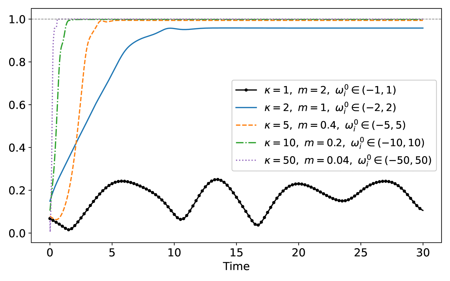
(a) Temporal evolution of $R$.

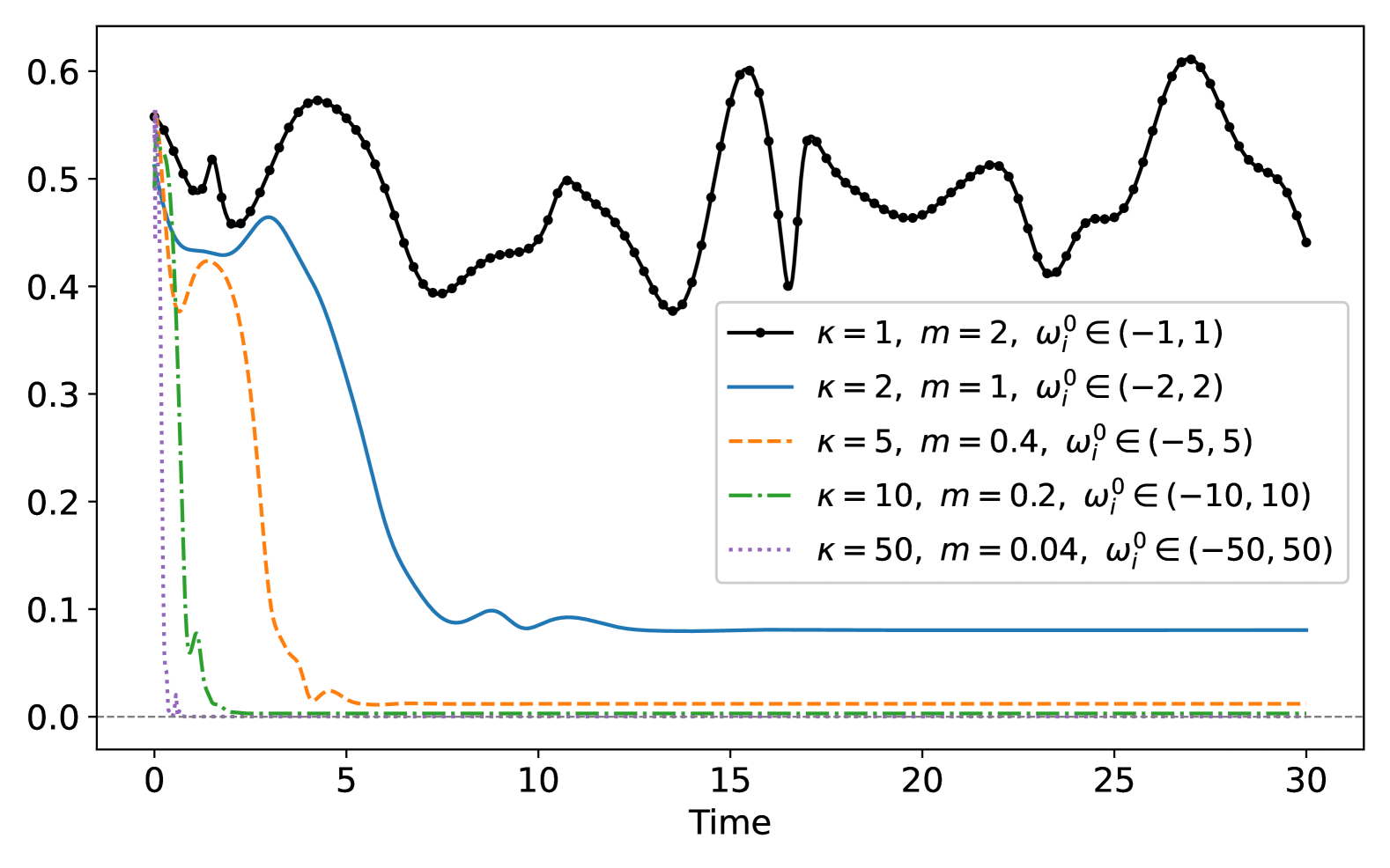
(b) Temporal evolution of $\Delta$.

Figure 1. (Color online) Simulations of $R$ and $\Delta$ varying ${\mathcal{D}}({\mathcal{V}})/\kappa$ and ${\mathcal{D}}(\Omega^{0})$. We used a single set of intrinsic frequency data uniformly distributed over the interval $[-1,1]$ for all simulations.

When $\mathcal{D}(\mathcal{V})/\kappa\leq\frac{1}{2}$, the limiting order parameter is close to $1$. Thus, it appears that the limiting configuration, which is a phase-locked state, is contained in a quarter circle. However, when $\mathcal{D}(\mathcal{V})/\kappa<1$, there is a unique phase-locked state for (1.1) and (2.1) in the quarter-circle; see [21] and Remark 2.4 (3). This phase-locked state may be computed from the equations

$$R=\frac{1}{N}\sum_{i=1}^{N}\cos(\theta_{i}-\phi),\quad\sin(\theta_{i}-\phi)=\frac{\nu_{i}-\nu_{c}}{\kappa R},\quad\forall i\in[N].$$

From the zeroth order approximation $R=1+o(1)$ (in the sense as $\mathcal{D}(\mathcal{V})/\kappa\to 0$), we have

$$\sin(\theta_{i}-\phi)=(1+o(1))\frac{\nu_{i}-\nu_{c}}{\kappa},$$

and

$$R=\frac{1}{N}\sum_{i=1}^{N}\sqrt{1-(1+o(1))\frac{(\nu_{i}-\nu_{c})^{2}}{\kappa^{2}}}=\frac{1}{N}\sum_{i=1}^{N}\left(1-\left(\frac{1}{2}+o(1)\right)\frac{(\nu_{i}-\nu_{c})^{2}}{\kappa^{2}}\right)=1-\left(\frac{1}{2}+o(1)\right)\frac{\operatorname{Var}(\mathcal{V})}{\kappa^{2}}.$$

Indeed, the values of $\frac{1-R(30)}{(\operatorname{Var}(\mathcal{V})/\kappa)^{2}}$ from the second to the fifth experiments in Figure 1 are 0.5676, 0.5089, 0.5022, 0.5001, respectively, and are close to 0.5.

What about the other factors? In Figure 2, we keep $\mathcal{D}(\mathcal{V})/\kappa$ and $\mathcal{D}(\Omega^{0})/\kappa$ constant and vary $m\kappa$. In this case, the same conclusion holds, i.e., the order parameter $R$ converges to a value close to $1$ while the mean-squared deviation $\Delta$ converges to a value close to $0$; the only difference is the time scale at which this happens, which is multiplicatively delayed proportional to $m$. This suggests that as long as $\mathcal{D}(\mathcal{V})/\kappa$ is small, variations in $m\kappa$ do not present material differences to the asymptotic dynamics.

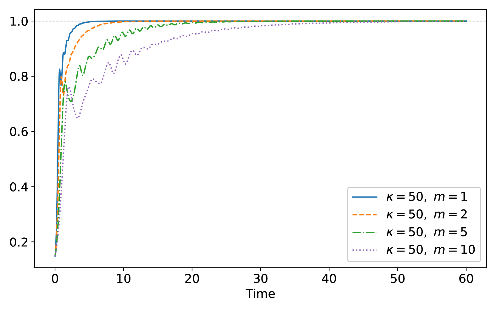
(a) Temporal evolution of $R$.

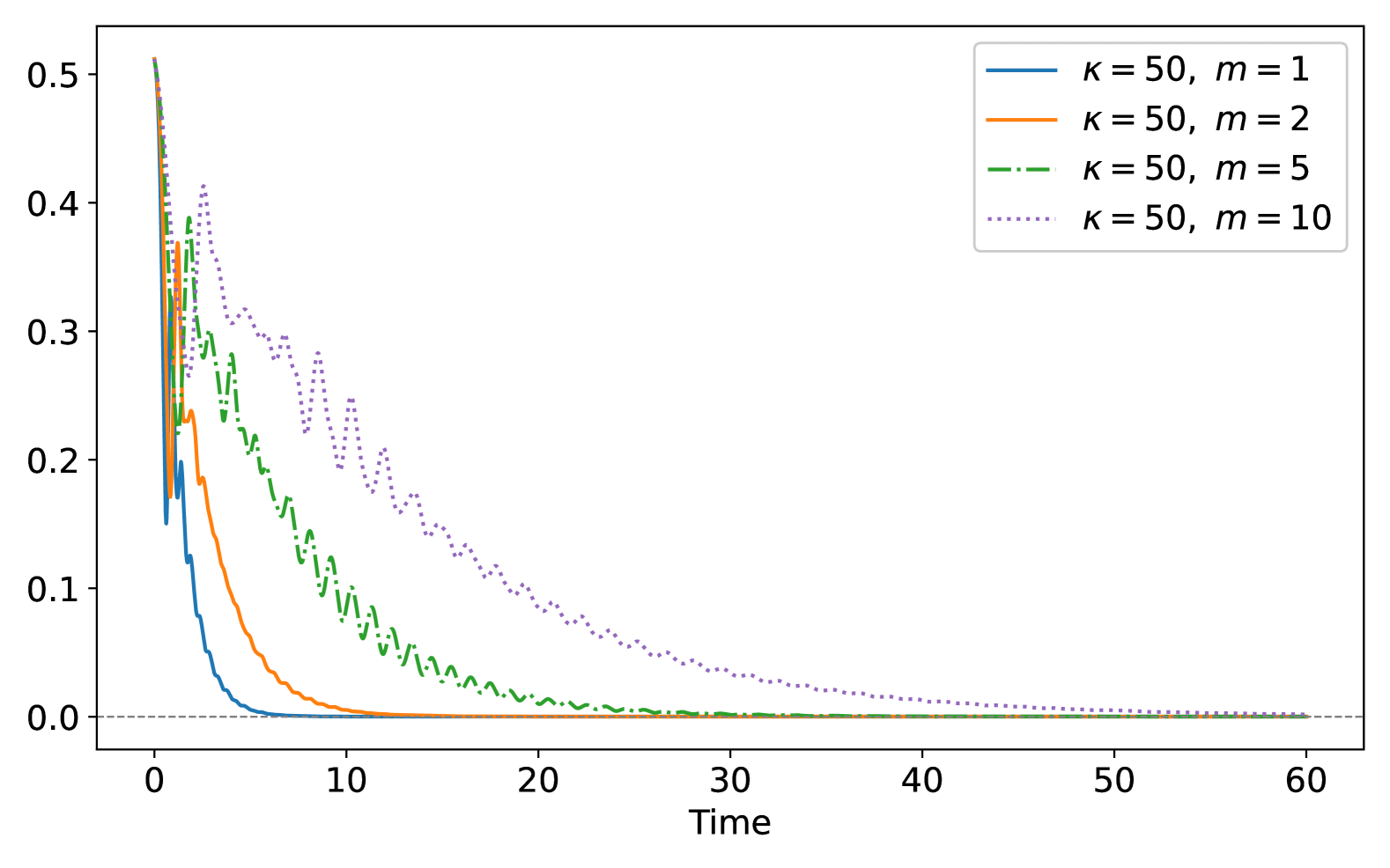
(b) Temporal evolution of $\Delta$.

Figure 2. (Color online) Simulations of $R$ and $\Delta$ varying $m\kappa$. We used a single set of initial frequency data and natural frequencies, uniformly distributed over the interval $[-1,1]$, for all simulations, respectively.

In Figure 3, we keep $\mathcal{D}(\mathcal{V})/\kappa$ and $m\kappa$ constant and vary $\mathcal{D}(\Omega^{0})/\kappa$. In this case, the same conclusion holds with the additively delayed time scale proportional to $m\mathcal{D}(W^{0})/\kappa$. Again, this suggests that as long as $\mathcal{D}(\mathcal{V})/\kappa$ is small, the magnitude of $\mathcal{D}(\Omega^{0})/\kappa$ does not significantly affect the asymptotic dynamics.

(a) Temporal evolution of $R$.

(b) Temporal evolution of $\Delta$.

Figure 3. (Color online) Simulations of $R$ and $\Delta$ varying ${\mathcal{D}}(\Omega^{0})/\kappa$. We used a single set of intrinsic frequency data uniformly distributed over the interval $[-1,1]$ for all simulations.

In summary, asymptotic phase-locking appears to occur if $\mathcal{D}(\mathcal{V})/\kappa$ is small, while the $m\kappa$ is the multiplicative time scale of the synchronization, and $\mathcal{D}(\Omega^{0})/\kappa$ acts as an additive delay for synchronization to happen. We collect our observations into the following conjecture.

Conjecture 4.2.

1. (Weak form) For any $\varepsilon>0$, there exists $\delta=\delta(\varepsilon)$ such that if $\mathcal{D}(\mathcal{V})/\kappa<\delta$, then for generic initial data $\Theta^{0}$, we have

   $$\liminf_{t\to\infty}R(t)\geq 1-\varepsilon.$$

2. (Strong form) For any $\varepsilon\in(0,\frac{1}{2})$, there exists a sufficiently small constant $c_{\varepsilon}>0$ such that $\operatorname{Var}(\mathcal{V})/\kappa<c_{\varepsilon}$, then for generic initial data $\Theta^{0}$, we have

   $$1-\left(\frac{1}{2}+\varepsilon\right)\frac{\operatorname{Var}(\mathcal{V})}{\kappa^{2}}\leq\liminf_{t\to\infty}R(t)\leq\limsup_{t\to\infty}R(t)\leq 1-\left(\frac{1}{2}-\varepsilon\right)\frac{\operatorname{Var}(\mathcal{V})}{\kappa^{2}}.$$

   If, in addition, $\mathcal{D}(\mathcal{V})/\kappa<c_{\varepsilon}$, then $\Theta(t)$ converges to the unique phase-locked state of (2.1) confined in the quarter circle [21].

Theorem 3.1 gives partial progress toward Conjecture 4.2 (1).

4.4. Piecing three mechanisms together

In this subsection, we summarize our strategy for the proof of Theorem 1.1, which is to combine three synchronization mechanisms of subsections 4.1, 4.2, and 4.3 together.

First, we briefly delineate our sufficient framework in terms of parameters and initial data. Compared to the simple conditions (2.2) for the Kuramoto model without inertia, our framework will be described by four free parameters $\lambda,\ell,\eta,\delta$. More precisely, the first two parameters, $\lambda$ and $\ell$, are the size and diameter of a majority phase cluster that will emerge from the given initial configuration in finite time. The third parameter $\eta$ is responsible for the range of the initial layer time zone $[0,\eta m]$. The last parameter $\delta$ is a lower bound for the ratio $R(t)/R^{0}$ in the initial layer time zone. The ranges of the above parameters can be summarized as follows.

$$\ell\in(0,\pi),\quad\lambda\in(0.5,1],\quad\eta\in(0,\infty),\quad\delta\in(0,1).$$

Now, we are ready to present our sufficient framework $\eqref{C-1}$: Let $(\Theta^{0},\Omega^{0})$ and ${\mathcal{V}}=\{\nu_{i}\}$ be given initial data and a set of natural frequencies. Then, we assume that the parameters and initial data satisfy the following set of conditions $({\mathcal{F}})$:

(4.20) $$\begin{cases}\displaystyle({\mathcal{F}}_{1}):~~R^{0}>0,\quad\zeta(\eta)\leq(1-\delta)R^{0}.\\ \displaystyle({\mathcal{F}}_{2}):~\delta R^{0}\geq\lambda+(1-\lambda)\cos\frac{\ell}{2}\quad\mathrm{or}\quad 2\lambda+\left(\frac{\xi(\eta)}{\delta R^{0}}\right)^{2}\frac{1}{1-\cos(\ell/2)}\leq 1+\delta R^{0}.\\ \displaystyle({\mathcal{F}}_{3}):~~\xi(\eta)<\sin\frac{\ell}{2}\left(\lambda\cos\frac{\ell}{2}-(1-\lambda)\right).\\ \displaystyle({\mathcal{F}}_{4}):~~\frac{\mathcal{D}(\mathcal{V})}{\kappa}+4m\kappa+2m\mathcal{D}(\mathcal{V})<\frac{(2\lambda-1)^{3/2}}{\sqrt{2\lambda}}\frac{2-\lambda}{\sqrt{\lambda/2}+(1-\lambda)}.\end{cases}$$

Here, $\zeta(\eta)=\zeta(m,\kappa,\mathcal{V},\Omega^{0},\eta)$ and $\xi(\eta)=\xi(m,\kappa,\mathcal{V},\Omega^{0},\eta)$ are dimensionless quantities defined in (4.17).

Note that condition $({\mathcal{F}}_{3})$ necessitates $\lambda\cos\frac{\ell}{2}-(1-\lambda)>0$. Framework $({\mathcal{F}})$ in $\eqref{C-1}$ is significantly different from those in the literature: framework (4.20) is the first to apply to generic initial data (the condition $R^{0}>0$ is satisfied for Lebesgue a.e. initial position data $\Theta^{0}$ in the position state space ${\mathbb{R}}^{N}$), not imposing any restriction on the cardinality or diameter of initial data.

Theorem 4.1.

Suppose the conditions $({\mathcal{F}}_{1})-({\mathcal{F}}_{3})$ hold, and let $(\Theta,\Omega)$ be a global solution to the Cauchy problem (3.6). Then the following assertions hold.

1. (Asymptotic phase-locking): There exists a constant state $\Theta^{\infty}\in{\mathbb{R}}^{N}$ such that

   $$\lim_{t\to\infty}\Big{(}\|\Theta(t)-\nu_{c}t{\bf 1}_{[N]}-{\Theta}^{\infty}\|_{\infty}+\|\Omega(t)-\nu_{c}{\bf 1}_{[N]}\|_{\infty}\Big{)}=0.$$

2. (Finite-time emergence and persistence of a majority cluster): There exist a nonnegative time $t_{*}>0$ and a subset $\mathcal{A}$ with $|\mathcal{A}|\geq\lambda N$ such that the majority cluster $\Theta_{\mathcal{A}}\coloneqq(\theta_{i})_{i\in\mathcal{A}}$ is confined modulo $2\pi$, after some time $t_{*}$, in an arc whose length is less than or equal to $\ell<\pi$; this means that there are integers $k_{i}$ for $i\in\mathcal{A}$ such that

   $$\mathcal{D}\left((\theta_{i}(t)-2k_{i}\pi)_{i\in\mathcal{A}}\right)<\ell,\quad t\geq t_{*}.$$

   There is a unique maximal (with respect to inclusion) such $\mathcal{A}$.

3. (Linear arrangement of majority cluster): If in addition (4.20)-(${\mathcal{F}}_{4}$) holds, then the majority cluster $\Theta_{\mathcal{A}}$ is arranged according to its natural frequencies: there is a constant $c$ depending only on $\frac{\mathcal{D}(\mathcal{V})}{\kappa}$, $m\kappa$, and $\lambda$ such that for any $i,j\in\mathcal{A}$ with $\nu_{i}\geq\nu_{j}$, we have

   $$\frac{\nu_{i}-\nu_{j}}{\kappa}\leq\lim_{t\to\infty}(\theta_{i}(t)-\theta_{j}(t)-2(k_{i}-k_{j})\pi)\leq c\frac{\nu_{i}-\nu_{j}}{\kappa}.$$

Proof.

We will prove statement (2) of Theorem 4.1 first in Section 7. Then, in Section 7, we will derive statement (1) of Theorem 4.1 from statement (2) using Proposition 4.1. On the other hand, the condition (4.20)-(${\mathcal{F}}_{4}$) enables us to tell an additional structural property, called linear arrangement, of the majority cluster described in (2) of Theorem 4.1. See Theorem 5.1. ∎

5. Partial phase-locking of majority clusters

In this section, we establish a version of this partial phase-locking result for the inertial Kuramoto model (1.1). We remark that a similar result has been established in [51] for the inertial Kuramoto model (1.1) (see Appendix A). We establish a stronger version of this theorem in this paper (see Corollary 5.1). Theorem A.1 in Section 5 says this is true for the first-order model (2.1). It tells us that not only these majority (i.e., $\lambda>\frac{1}{2}$) clusters are stable, but they can also control other certain oscillators as well. In what follows, we describe partial phase-locking in (1.1) due to majority clusters. For this, we begin by defining the function $f_{\lambda}:\mathbb{R}\rightarrow\mathbb{R}$ as

(5.1) $$f_{\lambda}(\theta)=2\sin\frac{\theta}{2}\left(\lambda\cos\frac{\theta}{2}-(1-\lambda)\right)=\lambda\sin\theta-2(1-\lambda)\sin\frac{\theta}{2},\quad\theta\in\mathbb{R},\quad\lambda\in\Big{(}\frac{1}{2},1\Big{]}.$$

Then $f_{\lambda}$ has the following properties.

Lemma 5.1 ([47, Lemma 4.2]).

The function $f_{\lambda}$ defined in (5.1) satisfies the following properties.

1. The function $f_{\lambda}$ has zeros at $\theta=0$ and $\theta=2\cos^{-1}\Big{(}\frac{1-\lambda}{\lambda}\Big{)}$, and is positive on the interval $\Big{(}0,2\cos^{-1}\frac{1-\lambda}{\lambda}\Big{)}$.

2. On the interval $(0,2\cos^{-1}\frac{1-\lambda}{\lambda})$, the function $f_{\lambda}$ is strictly concave and attains its maximum at the unique zero $\theta_{*}=2\cos^{-1}\Big{(}\frac{1-\lambda+\sqrt{(1-\lambda)^{2}+8\lambda^{2}}}{4\lambda}\Big{)}$ of $f_{\lambda}(\theta_{*})=0$ in $(0,2\cos^{-1}\frac{1-\lambda}{\lambda})$.

Thus, for $\delta\in(0,f_{\lambda}(\theta_{*}))$, the equation $f_{\lambda}(\theta)=\delta$ has two zeros $\phi_{1}=\phi_{1}(\lambda,\delta)$ and $\phi_{2}=\phi_{2}(\lambda,\delta)$ in $(0,2\cos^{-1}\frac{1-\lambda}{\lambda})$, with the ordering

(5.2) $$0<\phi_{1}<\theta_{*}<\phi_{2}<2\cos^{-1}\left(\frac{1-\lambda}{\lambda}\right).$$

These are the angles that the majority clusters will form.

Definition 5.1.

For $\lambda\in(1/2,1]$ and $\delta\in\mathbb{R}$ such that

$$0<\delta <\max_{\theta\in(0,2\cos^{-1}(\frac{1}{\lambda}-1))}f_{\lambda}(\theta)=f_{\lambda}(\theta_{*})$$

$$=\frac{\left(-3(1-\lambda)+\sqrt{9\lambda^{2}-2\lambda+1}\right)\sqrt{3\lambda^{2}+2\lambda-1-(1-\lambda)\sqrt{9\lambda^{2}-2\lambda+1}}}{4\sqrt{2}\lambda},$$

we denote by $\phi_{1}(\lambda,\delta)$ the smaller root and by $\phi_{2}(\lambda,\delta)$ the larger root among the two distinct roots of the following trigonometric equation in $\theta$:

$$\lambda\sin\theta-2(1-\lambda)\sin\frac{\theta}{2}=\delta,\quad\theta\in\left(0,2\cos^{-1}\frac{1-\lambda}{\lambda}\right).$$

In the next lemma, we collect some facts.

Lemma 5.2 ([47, Lemma 4.3]).

Let $\theta_{*},\phi_{1}$ and $\phi_{2}$ be defined as above. Then, the following estimates hold.

$$(i)~\phi_{1}<\frac{3\pi\delta}{4(2\lambda-1)},\quad\cos^{-1}\left(\frac{1-\lambda}{\lambda}\right)\leq\theta_{*}.$$

$$(ii)~f_{\lambda}\left(\cos^{-1}\frac{1-\lambda}{\lambda}\right)=\frac{(2\lambda-1)^{3/2}}{\sqrt{2\lambda}}\frac{2-\lambda}{\sqrt{\lambda/2}+(1-\lambda)}.$$

We state our partial-locking theorem for (1.1) as follows.

Theorem 5.1.

Suppose that the free real parameters $\lambda,\ell>0$ and index set ${\mathcal{A}}\subset[N]$ satisfy

(5.3) $$\frac{1}{2}<\lambda\leq 1,\quad\ell\in\left(0,2\cos^{-1}\Big{(}\frac{1}{\lambda}-1\Big{)}\right),\quad|\mathcal{A}|\geq\lambda N,$$

and that the system parameters and the free real parameter $\eta>0$ satisfy the following variant of (4.20)-$({\mathcal{F}}_{3})$ for the index set $\mathcal{A}\subset[N]$:

(5.4) $$\begin{aligned} \xi(m,\kappa,\mathcal{V}_{\mathcal{A}},\Omega^{0}_{\mathcal{A}},\eta)&=m\mathcal{D}(\mathcal{V}_{\mathcal{A}})+2m\kappa+\frac{\mathcal{D}(\mathcal{V}_{\mathcal{A}})}{2\kappa}\\ &+\mathcal{D}(\Omega^{0}_{\mathcal{A}})m\max\{1,\eta\}e^{-\max\{1,\eta\}}+\frac{\mathcal{D}(\Omega^{0}_{\mathcal{A}})}{2\kappa}\frac{e^{-\eta}}{1-e^{-\eta}}\\ &<\frac{\lambda}{2}\sin\ell-(1-\lambda)\sin\frac{\ell}{2},\end{aligned}$$

and let $(\Theta,\Omega)$ be a global solution to (3.6). Assume there exists a time $t_{1}\geq\eta m$ such that the subensemble $\Theta_{\mathcal{A}}=(\theta_{\ell})_{\ell\in\mathcal{A}}$ satisfies

$$\mathcal{D}(\Theta_{\mathcal{A}}(t_{1}))\leq\ell.$$

Then, the following assertions hold.

1. (Stability of the majority cluster): One has

   $$\sup_{t\geq t_{1}}\mathcal{D}(\Theta_{\mathcal{A}}(t))\leq\ell,$$

   and

   $$\begin{aligned} \limsup_{t\rightarrow\infty}\mathcal{D}(\Theta_{\mathcal{A}}(t))&\leq\phi_{1}\left(\lambda,2m\mathcal{D}(\mathcal{V}_{\mathcal{A}})+4m\kappa+\frac{\mathcal{D}(\mathcal{V}_{\mathcal{A}})}{\kappa}\right)\\ &\stackrel{{\scriptstyle\mathrm{Lemma~}\ref{f-estimates}(i)}}{{<}}\frac{3\pi}{4(2\lambda-1)}\left(2m\mathcal{D}(\mathcal{V}_{\mathcal{A}})+4m\kappa+\frac{\mathcal{D}(\mathcal{V}_{\mathcal{A}})}{\kappa}\right).\end{aligned}$$

2. (Partial linear arrangement) If we assume in addition that

   (5.5) $$2m\mathcal{D}(\mathcal{V}_{\mathcal{A}})+4m\kappa+\frac{\mathcal{D}(\mathcal{V}_{\mathcal{A}})}{\kappa}<\frac{(2\lambda-1)^{3/2}}{\sqrt{2\lambda}}\frac{2-\lambda}{\sqrt{\lambda/2}+(1-\lambda)},$$

   then the oscillators of $\Theta_{\mathcal{A}}$ becomes linearly ordered according to their natural frequencies: for $i,j\in\mathcal{A}$, with $\nu_{i}\geq\nu_{j}$,

   (5.6) $$\hskip 28.45274pt\frac{\nu_{i}-\nu_{j}}{\kappa}\leq\liminf_{t\rightarrow\infty}[\theta_{i}(t)-\theta_{j}(t)]\leq\limsup_{t\rightarrow\infty}[\theta_{i}(t)-\theta_{j}(t)]\leq\frac{\phi_{1}}{2\sin(\phi_{1}/2)(\lambda\cos\phi_{1}-(1-\lambda))}\frac{\nu_{i}-\nu_{j}}{\kappa},$$

   where $\phi_{1}=\phi_{1}\left(\lambda,2m\mathcal{D}(\mathcal{V}_{\mathcal{A}})+4m\kappa+\frac{\mathcal{D}(\mathcal{V}_{\mathcal{A}})}{\kappa}\right)$.

Now we assume that there is an index set $\mathcal{B}\subset[N]$ with $\mathcal{B}\supset\mathcal{A}$ satisfying the following variant of (5.4):

(5.7) $$\xi(m,\kappa,\mathcal{V}_{\mathcal{B}},\Omega^{0}_{\mathcal{B}},\infty)=m\mathcal{D}(\mathcal{V}_{\mathcal{B}})+2m\kappa+\frac{\mathcal{D}(\mathcal{V}_{\mathcal{B}})}{2\kappa}<\frac{\lambda}{2}\sin\ell-(1-\lambda)\sin\frac{\ell}{2}.$$

Then, the following statements hold.

1. (The majority cluster $\mathcal{A}$ confines $\mathcal{B}$) The ensemble $\Theta_{\mathcal{B}}$ is partially phase-locked:

   $$\sup_{t\geq 0}\mathcal{D}(\Theta_{\mathcal{B}}(t))<\infty.$$

   In particular, if $\mathcal{B}=[N]$, then asymptotic phase-locking occurs.

2. (Uniqueness of the maximal majority cluster) There is a unique index set $\mathcal{A}_{\mathrm{max}}\subset[N]$ with

   $$\mathcal{A}\subset\mathcal{A}_{\mathrm{max}}\subset\mathcal{B}$$

   possessing the following properties (a) and (b):

   1. (The ensemble $\Theta_{\mathcal{A}_{\mathrm{max}}}$ forms a cluster) By possibly replacing $\theta_{i}$ by $\theta_{i}-2k_{i}\pi$ for a suitable integer $k_{i}\in\mathbb{Z}$ over all $i\in\mathcal{A}_{\mathrm{max}}\setminus\mathcal{A}$, we have

      (5.8) $$\limsup_{t\rightarrow\infty}\mathcal{D}(\Theta_{\mathcal{A}_{\mathrm{max}}}(t))\leq\phi_{1}\left(\lambda,2m\mathcal{D}(\mathcal{V}_{\mathcal{B}})+4m\kappa+\frac{\mathcal{D}(\mathcal{V}_{\mathcal{B}})}{\kappa}\right).$$

   2. (Maximality and quantitative separation) Any enlargement of $\mathcal{A}_{\mathrm{max}}$ fails to form a cluster: if $\mathcal{A}_{\mathrm{max}}\subsetneq\mathcal{B}$, then

      (5.9) $$\liminf_{t\to\infty}\min_{\begin{subarray}{c}i\in\mathcal{B}\setminus\mathcal{A}_{\mathrm{max}}\\ k\in\mathbb{Z}\end{subarray}}\mathcal{D}(\Theta_{\mathcal{A}_{\mathrm{max}}}(t)\cup\{\theta_{i}(t)-2\pi k\})\geq\phi_{2}\left(\lambda,2m\mathcal{D}(\mathcal{V}_{\mathcal{B}})+4m\kappa+\frac{\mathcal{D}(\mathcal{V}_{\mathcal{B}})}{\kappa}\right),$$

      and we have the following separation estimate:

      (5.10) $$\begin{aligned} &\liminf_{t\to\infty}\min_{\begin{subarray}{c}i\in\mathcal{B}\setminus\mathcal{A}_{\mathrm{max}}\\ j\in\mathcal{A}_{\mathrm{max}}\\ k\in\mathbb{Z}\end{subarray}}|\theta_{i}(t)-2\pi k-\theta_{j}(t)|\\ &\hskip 28.45274pt\geq\phi_{2}\left(\lambda,2m\mathcal{D}(\mathcal{V}_{\mathcal{B}})+4m\kappa+\frac{\mathcal{D}(\mathcal{V}_{\mathcal{B}})}{\kappa}\right)-\phi_{1}\left(\lambda,2m\mathcal{D}(\mathcal{V}_{\mathcal{B}})+4m\kappa+\frac{\mathcal{D}(\mathcal{V}_{\mathcal{B}})}{\kappa}\right).\end{aligned}$$

   Again, under additional conditions, we have linear arrangement of $\Theta_{\mathcal{A}_{\mathrm{max}}}$:

   1. (Linear arrangement) If we assume in addition that

      $$2m\mathcal{D}(\mathcal{V}_{\mathcal{B}})+4m\kappa+\frac{\mathcal{D}(\mathcal{V}_{\mathcal{B}})}{\kappa}<\frac{(2\lambda-1)^{3/2}}{\sqrt{2\lambda}}\frac{2-\lambda}{\sqrt{\lambda/2}+(1-\lambda)},$$

      then the oscillators of $\Theta_{\mathcal{A}_{\mathrm{max}}}$ becomes, after suitable $2\pi$-translations, linearly ordered according to their natural frequencies: for $i,j\in\mathcal{A}_{\mathrm{max}}$, with $\nu_{i}\geq\nu_{j}$,

      $$\frac{\nu_{i}-\nu_{j}}{\kappa}\leq\liminf_{t\rightarrow\infty}[\theta_{i}(t)-\theta_{j}(t)]\leq\limsup_{t\rightarrow\infty}[\theta_{i}(t)-\theta_{j}(t)]\leq\frac{\phi_{1}}{2\sin(\phi_{1}/2)\left(\lambda\cos\phi_{1}-(1-\lambda)\right)}\frac{\nu_{i}-\nu_{j}}{\kappa},$$

      where $\phi_{1}=\phi_{1}\left(\lambda,2m\mathcal{D}(\mathcal{V}_{\mathcal{B}})+4m\kappa+\frac{\mathcal{D}(\mathcal{V}_{\mathcal{B}})}{\kappa}\right)$.

Proof.

Since the proofs are very lengthy, we leave them in the following subsections. ∎

Remark 5.1.

Below, we comment on the contents of serval assertions appearing in Theorem 5.1. We refer to Theorem A.1 in Appendix A.1 for a version of Theorem 5.1 in the simpler case of the first-order model (2.1). The assertions in Theorem 5.1 can be rephrased as follows.

1. Once a majority $\mathcal{A}$ of the phase oscillators is concentrated (modulo $2\pi$) in an arc of sufficiently small length $\ell$ at some finite time $t_{1}\geq\eta m$ bounded away from $0$, they must always stay in an arc of length at most $\ell$ after that time if the coupling strength is sufficiently large compared to $\mathcal{D}(\mathcal{V})$, $\mathcal{D}(\Omega^{0})$, and $1/m$. Thus, $\mathcal{A}$ becomes a stable majority cluster.

2. With stronger assumptions on the smallness of the normalized natural frequency diameter $\mathcal{D}(\mathcal{V}_{\mathcal{A}})/\kappa$ and normalized inertia $m\kappa$, the members of the majority cluster $\mathcal{A}$ eventually rearrange themselves according to the linear order of their natural frequencies $\nu_{i}$.

3. The movement of other members in $\mathcal{B}\setminus\mathcal{A}$ is heavily restricted by the majority cluster $\mathcal{A}$, since they become part of the majority cluster $\mathcal{A}$ if they cross paths with them.

4. The members of $\mathcal{B}$ which join the majority cluster $\mathcal{A}$ attract each other as well. This allows us to identify a unique maximal majority cluster $\mathcal{A}_{\mathrm{max}}$ with $\mathcal{A}\subset\mathcal{A}_{\mathrm{max}}\subset\mathcal{B}$, from which $\mathcal{B}\setminus\mathcal{A}_{\mathrm{max}}$ distances itself.

Simply put, a concentrated majority cluster is stable and attractive.

As an application of Theorem 5.1, we use the finite speed of (3.6) to show the stability of majority clusters for initial data as follows.

Corollary 5.1.

Suppose that the free real parameters $\lambda,\ell$ satisfy

$$\frac{1}{2}<\lambda\leq 1,\quad\ell\in\left(0,2\cos^{-1}\left(\frac{1}{\lambda}-1\right)\right),$$

and that the system parameters, free real parameter $\eta>0$, and index set $\mathcal{A}\subset[N]$ satisfy $|\mathcal{A}|\geq\lambda N$, (5.4), and

$$\mathcal{D}(\Theta_{\mathcal{A}}^{0})\leq\ell-m(1-e^{-\eta})\mathcal{D}(\Omega_{\mathcal{A}})-(\eta m-m+me^{-\eta})(\mathcal{D}(\mathcal{V}_{\mathcal{A}})+2\kappa),$$

and let $(\Theta,\Omega)$ be a global solution to (3.6). Then, the conclusion of Theorem 5.1 holds with $t_{1}=\eta m$.

Proof.

By Lemma 3.1 (2), we have that for $i,j\in\mathcal{A}$ and $t\geq 0$,

$$|\dot{\theta}_{i}-\dot{\theta}_{j}|\leq e^{-t/m}|\omega_{i}^{0}-\omega_{j}^{0}|+(1-e^{-t/m})(|\nu_{i}-\nu_{j}|+2\kappa)\leq e^{-t/m}\mathcal{D}(\Omega_{\mathcal{A}})+(1-e^{-t/m})(\mathcal{D}(\mathcal{V}_{\mathcal{A}})+2\kappa)$$

and hence, we have

$$\mathcal{D}(\Theta_{\mathcal{A}}(\eta m))-\mathcal{D}(\Theta_{\mathcal{A}}^{0}) \leq\int_{0}^{\eta m}\left(e^{-t/m}\mathcal{D}(\Omega_{\mathcal{A}})+(1-e^{-t/m})(\mathcal{D}(\mathcal{V}_{\mathcal{A}})+2\kappa)\right)dt$$

$$=m(1-e^{-\eta})\mathcal{D}(\Omega_{\mathcal{A}})+(\eta m-m+me^{-\eta})(\mathcal{D}(\mathcal{V}_{\mathcal{A}})+2\kappa).$$

By the condition of corollary, we have

$$\mathcal{D}(\Theta_{\mathcal{A}}(\eta m))\leq\ell.$$

Then, we may apply Theorem 5.1 with $t_{1}=\eta m$ to get the desired estimate. ∎

Remark 5.2.

In general, even though the subensemble $\Theta_{\mathcal{A}}$, viewed as particles on the unit circle $\mathbb{S}^{1}$, may lie on a small arc on the circle, it need not be the case when they are viewed as particles on the real line $\mathbb{R}$. See Figure 4 for a demonstration of this phenomenon. Nevertheless, owing to the $2\pi\mathbb{Z}$-translation invariance of (1.1), Theorem 5.1 may be employed harmlessly for our purposes of proving partial or asymptotic phase-locking whenever we have that $\Theta_{\mathcal{A}}$ lies on a small arc on the circle.

(a) Geometric configuration on $\mathbb{R}^{1}$.

(b) Geometric configuration on $\mathbb{T}^{1}$.

Figure 4. Schematic descriptions for virtual rearrangement; $\theta_{s}$ and $\theta_{r}$ are on the same arc on ${\mathbb{T}}^{1}$ but may not be in the same on ${\mathbb{R}}^{1}$. Considering $2\pi k_{s}$ translation (for some $k_{s}$) enable us to regard $\tilde{\theta}_{s}\coloneqq\theta_{s}-2k_{s}\pi$ as $\theta_{s}$ in our estimations.

We are now ready to prove several assertions in Theorem 5.1 one by one.

5.1. Proof of the first assertion in Theorem 5.1 (Stability of $\Theta_{\mathcal{A}}$)

In this subsection, we show the first assertion that the majority cluster formed at $t=t_{1}\geq\eta m$ persists afterwards.

Recall that there exists an index set $\mathcal{A}$ with $|\mathcal{A}|\geq\lambda N$ such that the corresponding subensemble $\Theta_{\mathcal{A}}=(\theta_{i})_{i\in\mathcal{A}}$ satisfies

$$\mathcal{D}(\Theta_{\mathcal{A}}(t_{1}))\leq\ell,$$

for some $t_{1}\geq\eta m$. Next, we show that

(5.11) $${\mathcal{D}}(\Theta_{\mathcal{A}}(t))\leq\ell,\quad\forall t\geq t_{1},$$

and

(5.12) $$\limsup_{t\to\infty}\mathcal{D}(\Theta_{\mathcal{A}}(t))\leq\phi_{1}\left(\lambda,2m\mathcal{D}(\mathcal{V}_{\mathcal{A}})+4m\kappa+\frac{\mathcal{D}(\mathcal{V}_{\mathcal{A}})}{\kappa}\right).$$

By definition of $f_{\lambda}$, condition (5.4) becomes

$$2\xi(m,\kappa,\mathcal{V}_{\mathcal{A}},\Omega^{0}_{\mathcal{A}},\eta)<f_{\lambda}(\ell),$$

and since $f_{\lambda}$ has its maximum in $\Big{[}0,2\cos^{-1}\frac{1-\lambda}{\lambda}\Big{]}$ at $\theta_{*}$, we also have

$$2\xi(m,\kappa,\mathcal{V}_{\mathcal{A}},\Omega^{0}_{\mathcal{A}},\eta)<f_{\lambda}(\theta_{*}).$$

By Lemma 5.1, the equation $f_{\lambda}(\theta)=2\xi(m,\kappa,\mathcal{V}_{\mathcal{A}},\Omega^{0}_{\mathcal{A}},\eta)$ has two zeros $\theta=\phi_{1}(\eta)$ and $\theta=\phi_{2}(\eta)$ in the interval $(0,2\cos^{-1}\frac{1-\lambda}{\lambda})$, which, by the strict concavity of $f_{\lambda}$, have the ordering

$$0<\phi_{1}(\eta)<\ell<\phi_{2}(\eta)<2\cos^{-1}\left(\frac{1-\lambda}{\lambda}\right).$$

Choose any $\psi_{1},\psi_{2}\in\mathbb{R}$ with

(5.13) $$\phi_{1}(\eta)<\psi_{1}\leq\ell\leq\psi_{2}<\phi_{2}(\eta),\quad\psi_{1}<\psi_{2}.$$

Again by the strict concavity of $f_{\lambda}$, there exists a positive constant $c>0$ such that

(5.14) $$2\xi(m,\kappa,\mathcal{V}_{\mathcal{A}},\Omega^{0}_{\mathcal{A}},\eta)+c<f_{\lambda}(\theta),\quad\theta\in[\psi_{1},\psi_{2}].$$

We will show that whenever $\mathcal{D}(\Theta_{\mathcal{A}})\in[\psi_{1},\psi_{2}]$ on the time interval $[t_{1},\infty)$, it has a negative upper Dini (time) derivative: $D^{+}\mathcal{D}(\Theta_{\mathcal{A}})<0$. Note that we may compute the upper Dini derivative as follows:

(5.15) $$D^{+}\mathcal{D}(\Theta_{\mathcal{A}})=\max_{\begin{subarray}{c}i,j\in\mathcal{A}\\ \theta_{i}=\max_{k\in\mathcal{A}}\theta_{k}\\ \theta_{j}=\min_{k\in\mathcal{A}}\theta_{k}\end{subarray}}\left(\dot{\theta}_{i}-\dot{\theta}_{j}\right)$$

By Invoking Lemma 3.2, for $i,j\in\mathcal{A}$ we have

$$\dot{\theta}_{i}(t)-\dot{\theta}_{j}(t)\leq\frac{\kappa\left(1-e^{-t/m}\right)}{N}\sum_{l\in\mathcal{A}}\left(\sin(\theta_{l}(t)-\theta_{i}(t))-\sin(\theta_{l}(t)-\theta_{j}(t))\right)$$

$$\hskip 19.91684pt+(\omega^{0}_{i}-\omega^{0}_{j})e^{-t/m}+(\nu_{i}-\nu_{j})(1-e^{-t/m})$$

$$\hskip 19.91684pt+2\kappa\left(\mathcal{D}(\Omega^{0}_{\mathcal{A}})te^{-t/m}\left(1-e^{-t/m}\right)+m(\mathcal{D}(\mathcal{V}_{\mathcal{A}})+2\kappa)\left(1-e^{-t/m}\right)^{3}\right)$$

$$\hskip 19.91684pt+\frac{N-|\mathcal{A}|}{N}2\kappa\left|\sin\frac{\theta_{i}(t)-\theta_{j}(t)}{2}\right|\left(1-e^{-t/m}\right)$$

$$\hskip 19.91684pt\leq-\frac{2\kappa\left(1-e^{-t/m}\right)}{N}\sin\frac{\theta_{i}(t)-\theta_{j}(t)}{2}\sum_{l\in\mathcal{A}}\cos\left(\theta_{l}(t)-\frac{\theta_{i}(t)+\theta_{j}(t)}{2}\right)$$

$$\hskip 19.91684pt+\mathcal{D}(\Omega^{0}_{\mathcal{A}})e^{-t/m}+\mathcal{D}(\mathcal{V}_{\mathcal{A}})(1-e^{-t/m})$$

$$\hskip 19.91684pt+2\kappa\left(\mathcal{D}(\Omega^{0}_{\mathcal{A}})te^{-t/m}\left(1-e^{-t/m}\right)+m(\mathcal{D}(\mathcal{V}_{\mathcal{A}})+2\kappa)\left(1-e^{-t/m}\right)^{3}\right)$$

$$\hskip 19.91684pt+\frac{N-|\mathcal{A}|}{N}2\kappa\left|\sin\frac{\theta_{i}(t)-\theta_{j}(t)}{2}\right|\left(1-e^{-t/m}\right).$$

If $t\geq t_{1}$ is such that $\mathcal{D}(\Theta_{\mathcal{A}}(t))\leq\pi$, and $i,j\in\mathcal{A}$ are so that

$$\theta_{i}(t)=\max_{k\in\mathcal{A}}\theta_{k}(t)\quad\mbox{and}\quad\theta_{j}(t)=\min_{k\in\mathcal{A}}\theta_{k}(t),$$

then we have

$$\cos\left(\theta_{l}(t)-\frac{\theta_{i}(t)+\theta_{j}(t)}{2}\right)\geq\cos\frac{\theta_{i}(t)-\theta_{j}(t)}{2},\quad l\in\mathcal{A},$$

so that, continuing the above estimate and $|\mathcal{A}|\geq\lambda N$,

$$\dot{\theta}_{i}(t)-\dot{\theta}_{j}(t)\leq -2\lambda\kappa\left(1-e^{-t/m}\right)\sin\frac{\theta_{i}(t)-\theta_{j}(t)}{2}\cos\frac{\theta_{i}(t)-\theta_{j}(t)}{2}$$

$$+\mathcal{D}(\Omega^{0}_{\mathcal{A}})e^{-t/m}+\mathcal{D}(\mathcal{V}_{\mathcal{A}})(1-e^{-t/m})$$

$$+2\kappa\left(\mathcal{D}(\Omega^{0}_{\mathcal{A}})te^{-t/m}\left(1-e^{-t/m}\right)+m(\mathcal{D}(\mathcal{V}_{\mathcal{A}})+2\kappa)\left(1-e^{-t/m}\right)^{3}\right)$$

$$+(1-\lambda)2\kappa\sin\frac{\theta_{i}(t)-\theta_{j}(t)}{2}\left(1-e^{-t/m}\right)$$

$$\leq -2\kappa\left(1-e^{-t/m}\right)\sin\frac{\theta_{i}(t)-\theta_{j}(t)}{2}\left(\lambda\cos\frac{\theta_{i}(t)-\theta_{j}(t)}{2}-(1-\lambda)\right)$$

$$+\mathcal{D}(\Omega^{0}_{\mathcal{A}})e^{-t/m}+\mathcal{D}(\mathcal{V}_{\mathcal{A}})(1-e^{-t/m})$$

$$+2\kappa\left(\mathcal{D}(\Omega^{0}_{\mathcal{A}})te^{-t/m}\left(1-e^{-t/m}\right)+m(\mathcal{D}(\mathcal{V}_{\mathcal{A}})+2\kappa)\left(1-e^{-t/m}\right)^{3}\right).$$

Again, by Invoking (5.15), we have

$$\left.D^{+}\right|_{t}\mathcal{D}(\Theta_{\mathcal{A}})\leq -2\kappa\left(1-e^{-t/m}\right)\sin\frac{\mathcal{D}(\Theta_{\mathcal{A}}(t))}{2}\left(\lambda\cos\frac{\mathcal{D}(\Theta_{\mathcal{A}}(t))}{2}-(1-\lambda)\right)$$

$$+\mathcal{D}(\Omega^{0}_{\mathcal{A}})e^{-t/m}+\mathcal{D}(\mathcal{V}_{\mathcal{A}})(1-e^{-t/m})$$

$$+2\kappa\left(\mathcal{D}(\Omega^{0}_{\mathcal{A}})te^{-t/m}\left(1-e^{-t/m}\right)+m(\mathcal{D}(\mathcal{V}_{\mathcal{A}})+2\kappa)\left(1-e^{-t/m}\right)^{3}\right)$$

$$\leq -\kappa\left(1-e^{-t/m}\right)\left(f_{\lambda}(\mathcal{D}(\Theta_{\mathcal{A}}(t)))-2\xi(m,\kappa,\mathcal{V}_{\mathcal{A}},\Omega^{0}_{\mathcal{A}},\eta)\right).$$

Now, if time $t_{0}\geq t_{1}$ is such that

$$\mathcal{D}(\Theta_{\mathcal{A}}(t_{0}))\in[\psi_{1},\psi_{2}],$$

where $\psi_{1},\psi_{2}$ are as in (5.13), then, by (5.14), we have

$$\left.D^{+}\right|_{t_{0}}\mathcal{D}(\Theta_{\mathcal{A}})\leq-\kappa\left(1-e^{-t/m}\right)c<0.$$

By a standard exit-time argument, we can easily establish that

$$D(\Theta_{\mathcal{A}}(t))\leq\ell,\quad\forall t\geq t_{1},$$

i.e., we have (5.11), and we can establish that there is a finite time $T\geq t_{1}$ with $T\leq t_{1}+\frac{\psi_{2}-\psi_{1}}{\kappa\left(1-e^{-t/m}\right)c}$ such that

$$D(\Theta_{\mathcal{A}}(t))\leq\psi_{1},\quad\forall t\geq T.$$

Since $\psi_{1}\in(\phi_{1}(\lambda,2\xi(m,\kappa,\mathcal{V}_{\mathcal{A}},\Omega^{0}_{\mathcal{A}},\eta)),\ell)$ was arbitrary, we conclude that

(5.16) $$\limsup_{t\rightarrow\infty}D(\Theta_{\mathcal{A}}(t))\leq\phi_{1}(\lambda,2\xi(m,\kappa,\mathcal{V}_{\mathcal{A}},\Omega^{0}_{\mathcal{A}},\eta)).$$

So far, we have shown that under the assumptions of Theorem 5.1, we have (5.11) and (5.16). Let $\eta^{\prime}\geq\eta$ be arbitrary. By (5.11), we have

$$\mathcal{D}(\Theta_{\mathcal{A}}(t_{1}^{\prime}))\leq\ell$$

for $t_{1}^{\prime}=\max\{t_{1},\eta^{\prime}m\}\geq\eta^{\prime}m$, and since the map $\eta\mapsto\xi(\eta)$ is decreasing, we have

$$\xi(m,\kappa,\mathcal{V}_{\mathcal{A}},\Omega^{0}_{\mathcal{A}},\eta^{\prime})\leq\xi(m,\kappa,\mathcal{V}_{\mathcal{A}},\Omega^{0}_{\mathcal{A}},\eta)<\frac{\lambda}{2}\sin\ell-(1-\lambda)\sin\frac{\ell}{2}.$$

So the assumptions of Theorem 5.1 are satisfied with $\eta$ replaced by $\eta^{\prime}$ and $t_{1}$ replaced by $t_{1}^{\prime}$, and we have (5.16) for $\eta^{\prime}$:

$$\limsup_{t\rightarrow\infty}\mathcal{D}(\Theta_{\mathcal{A}}(t))\leq\phi_{1}(\lambda,2\xi(m,\kappa,\mathcal{V}_{\mathcal{A}},\Omega^{0}_{\mathcal{A}},\eta^{\prime})).$$

Since $\eta^{\prime}\geq\eta$ was arbitrary, take the limit $\eta^{\prime}\to\infty$ to obtain

$$\limsup_{t\rightarrow\infty}\mathcal{D}(\Theta_{\mathcal{A}}(t))\leq\phi_{1}(\lambda,2\xi(m,\kappa,\mathcal{V}_{\mathcal{A}},\Omega^{0}_{\mathcal{A}},\infty)),$$

which is (5.12). This completes the proof of the first assertion.

5.2. Proof of the second assertion in Theorem 5.1 (Linear arrangement of $\Theta_{{\mathcal{A}}}$)

Now we assume in addition that the following relations (5.5) hold:

$$2m\mathcal{D}(\mathcal{V}_{\mathcal{A}})+4m\kappa+\frac{\mathcal{D}(\mathcal{V}_{\mathcal{A}})}{\kappa}<\frac{(2\lambda-1)^{3/2}}{\sqrt{2\lambda}}\frac{2-\lambda}{\sqrt{\lambda/2}+(1-\lambda)}.$$

We claim that the following relations holds:  for $i,j\in\mathcal{A}$, with $\nu_{i}\geq\nu_{j}$, we have

$$\frac{\nu_{i}-\nu_{j}}{\kappa}\leq\liminf_{t\rightarrow\infty}[\theta_{i}(t)-\theta_{j}(t)]\leq\limsup_{t\rightarrow\infty}[\theta_{i}(t)-\theta_{j}(t)]\leq\frac{\phi_{1}}{2\sin(\phi_{1}/2)\left(\lambda\cos\phi_{1}-(1-\lambda)\right)}\frac{\nu_{i}-\nu_{j}}{\kappa},$$

where $\phi_{1}=\phi_{1}\left(\lambda,2m\mathcal{D}(\mathcal{V}_{\mathcal{A}})+4m\kappa+\frac{\mathcal{D}(\mathcal{V}_{\mathcal{A}})}{\kappa}\right)$.

Recall (5.12):

(5.12) $$\limsup_{t\to\infty}\mathcal{D}(\Theta_{\mathcal{A}}(t))\leq\phi_{1}\left(\lambda,2m\mathcal{D}(\mathcal{V}_{\mathcal{A}})+4m\kappa+\frac{\mathcal{D}(\mathcal{V}_{\mathcal{A}})}{\kappa}\right).$$

Since we have $\phi_{1}\leq\theta_{*}$ by (5.2), $\cos^{-1}\frac{1-\lambda}{\lambda}\leq\theta_{*}$ by Lemma 5.2, and since $f_{\lambda}$ is strictly increasing on $[0,\theta_{*}]$, we have the following equivalence:

(5.17) $$\phi_{1}\left(\lambda,2m\mathcal{D}(\mathcal{V}_{\mathcal{A}})+4m\kappa+\frac{\mathcal{D}(\mathcal{V}_{\mathcal{A}})}{\kappa}\right)<\cos^{-1}\Big{(}\frac{1-\lambda}{\lambda}\Big{)}$$

$$\hskip 14.22636pt\Longleftrightarrow\quad f_{\lambda}\left(\phi_{1}\left(\lambda,2m\mathcal{D}(\mathcal{V}_{\mathcal{A}})+4m\kappa+\frac{\mathcal{D}(\mathcal{V}_{\mathcal{A}})}{\kappa}\right)\right)<f_{\lambda}\left(\cos^{-1}\left(\frac{1-\lambda}{\lambda}\right)\right)$$

$$\hskip 14.22636pt\Longleftrightarrow\quad 2m\mathcal{D}(\mathcal{V}_{\mathcal{A}})+4m\kappa+\frac{\mathcal{D}(\mathcal{V}_{\mathcal{A}})}{\kappa}<\frac{(2\lambda-1)^{3/2}}{\sqrt{2\lambda}}\frac{2-\lambda}{\sqrt{\lambda/2}+(1-\lambda)}\quad(\because\mathrm{Lemma~\ref{f-estimates}~(ii)})$$

$$\hskip 14.22636pt\Longleftrightarrow\quad\eqref{additional0},$$

so every statement here, in particular the first statement, is true. Let

(5.18) $$\psi_{1}\in\left(\phi_{1}\left(\lambda,2m\mathcal{D}(\mathcal{V}_{\mathcal{A}})+4m\kappa+\frac{\mathcal{D}(\mathcal{V}_{\mathcal{A}})}{\kappa}\right),\cos^{-1}\frac{1-\lambda}{\lambda}\right)$$

be arbitrary. By (5.12), there exists a finite time $T\geq t_{1}$ such that

(5.19) $$D(\Theta_{\mathcal{A}}(t))\leq\psi_{1},\quad\forall~t\geq T,$$

Let $i,j\in\mathcal{A}$ and $t\geq T$. Because we are looking in the long-term with the a priori guarantee that $\theta_{i}$ and $\theta_{j}$ are always contained in an $\ell$-arc for times $t\geq t_{1}$, we need not be restrained by the myopic approach of the previous subsection, i.e., estimating $\dot{\Theta}_{\mathcal{A}}(t)$ from $\Theta_{\mathcal{A}}(t)$ and $\dot{\Theta}_{\mathcal{A}}^{0}$. Instead, we may employ the second-order ODE directly:

(5.20) $$\begin{aligned} m(\ddot{\theta}_{i}-\ddot{\theta}_{j})+\dot{\theta}_{i}-\dot{\theta}_{j}&=\nu_{i}-\nu_{j}+\frac{\kappa}{N}\sum_{k=1}^{N}\left[\sin(\theta_{k}-\theta_{i})-\sin(\theta_{k}-\theta_{j})\right]\\ &=\nu_{i}-\nu_{j}-2\kappa\sin\Big{(}\frac{\theta_{i}-\theta_{j}}{2}\Big{)}\cdot\frac{1}{N}\sum_{k=1}^{N}\cos\left(\theta_{k}-\frac{\theta_{i}+\theta_{j}}{2}\right),\end{aligned}$$

where

(5.21) $$-1\leq\frac{1}{N}\sum_{k=1}^{N}\cos\left(\theta_{k}-\frac{\theta_{i}+\theta_{j}}{2}\right)\leq 1$$

and (recalling the assumption $t\geq T$)

(5.22) $$\begin{aligned} \frac{1}{N}\sum_{k=1}^{N}\cos\left(\theta_{k}-\frac{\theta_{i}+\theta_{j}}{2}\right)&=\frac{1}{N}\sum_{k\in\mathcal{A}}\cos\left(\theta_{k}-\frac{\theta_{i}+\theta_{j}}{2}\right)+\frac{1}{N}\sum_{k\in[N]\backslash\mathcal{A}}\cos\left(\theta_{k}-\frac{\theta_{i}+\theta_{j}}{2}\right)\\ &\geq\frac{|\mathcal{A}|}{N}\cos\mathcal{D}(\Theta_{\mathcal{A}})-\frac{N-|\mathcal{A}|}{N}\geq\lambda\cos\mathcal{D}(\Theta_{\mathcal{A}})-(1-\lambda).\end{aligned}$$

The penultimate inequality uses the fact that since

$$\mathcal{D}(\Theta_{\mathcal{A}}(t))\stackrel{{\scriptstyle\mathclap{\eqref{trapped}}}}{{\leq}}\psi_{1}<\cos^{-1}\frac{1-\lambda}{\lambda}\leq\frac{\pi}{2},$$

we have

$$\cos\left(\theta_{k}-(\theta_{i}+\theta_{j})/2\right)\geq\cos\mathcal{D}(\Theta_{\mathcal{A}})\quad\forall~i,j,k\in\mathcal{A}.$$

Note that since we are not assuming that $\theta_{i}$ and $\theta_{j}$ are extremal in $\Theta_{\mathcal{A}}$ as before, we cannot say that

$$\left|\theta_{k}-\frac{\theta_{i}+\theta_{j}}{2}\right|\leq\frac{D(\Theta_{\mathcal{A}})}{2},$$

but we can only say that

$$\left|\theta_{k}-\frac{\theta_{i}+\theta_{j}}{2}\right|\leq D(\Theta_{\mathcal{A}}).$$

The final inequality uses the fact that $1+\cos\mathcal{D}(\Theta_{\mathcal{A}})\geq 0$.

Note that our assumption (5.5), which implies (5.17). This allows the choice of $\psi_{1}$ as in (5.18) and it tells us that (5.22) is positive:

(5.23) $$\frac{1}{N}\sum_{k=1}^{N}\cos\left(\theta_{k}-\frac{\theta_{i}+\theta_{j}}{2}\right)~\stackrel{{\scriptstyle\mathclap{\eqref{crude-mf}}}}{{\geq}}\lambda\cos D(\Theta_{\mathcal{A}})-(1-\lambda)\stackrel{{\scriptstyle\mathclap{\eqref{eq:psi-choice}}}}{{\geq}}\lambda\cos\psi_{1}-(1-\lambda)~\stackrel{{\scriptstyle\mathclap{\eqref{eq:psi-choice}}}}{{>}}~0,\quad\forall t\geq T.$$

With the estimates (5.21) and (5.23) on the mean-field term at our disposal, we are now ready to prove the desired statement. Next, we consider two cases: $\nu_{i}=\nu_{j}$ or $\nu_{i}>\nu_{j}$.

$\diamond$ Case A ($\nu_{i}=\nu_{j}$): In this case, (5.20) becomes

$$m(\ddot{\theta}_{i}-\ddot{\theta}_{j})+\dot{\theta}_{i}-\dot{\theta}_{j}=-\frac{2\kappa}{N}\sum_{k=1}^{N}\cos\left(\theta_{k}-\frac{\theta_{i}+\theta_{j}}{2}\right)\cdot\sin\frac{\theta_{i}-\theta_{j}}{2},\quad t\geq T.$$

Thus, for a time interval $J\subset[T,\infty)$ on which $\theta_{i}-\theta_{j}>0$, we have

$$\theta_{i}-\theta_{j}\in\left(0,\frac{\pi}{2}\right)\quad\mbox{and}\quad m(\ddot{\theta}_{i}-\ddot{\theta}_{j})+\dot{\theta}_{i}-\dot{\theta}_{j}\stackrel{{\scriptstyle\eqref{crude-mf0}}}{{\geq}}-2\kappa\sin\frac{\theta_{i}-\theta_{j}}{2}>-\kappa(\theta_{i}-\theta_{j}).$$

Likewise, for a time interval $J\subset[T,\infty)$ on which $\theta_{i}-\theta_{j}<0$, we have

$$\theta_{i}-\theta_{j}\in\left(-\frac{\pi}{2},0\right)\quad\mbox{and}\quad m(\ddot{\theta}_{i}-\ddot{\theta}_{j})+\dot{\theta}_{i}-\dot{\theta}_{j}\stackrel{{\scriptstyle\eqref{crude-mf0}}}{{\leq}}-2\kappa\sin\frac{\theta_{i}-\theta_{j}}{2}<-\kappa(\theta_{i}-\theta_{j}).$$

Note also that $m\kappa<\frac{1}{4}$, which follows from (5.4):

$$2m\kappa\leq\xi(m,\kappa,\mathcal{V}_{\mathcal{A}},\Omega^{0}_{\mathcal{A}},\eta)\stackrel{{\scriptstyle\eqref{eq:xi-partial}}}{{<}}\frac{\lambda}{2}\sin\ell-(1-\lambda)\sin\frac{\ell}{2}\leq\frac{1}{2}.$$

Therefore, $y=\theta_{i}-\theta_{j}$ satisfies the hypothesis of statement (3) of Lemma B.1, with $I=(T,\infty)$, $a=m$, $b=1$, and $c=\kappa$. It follows that $\theta_{i}-\theta_{j}$ cannot change sign twice in $(T,\infty)$, so that there exists a time $t_{2}\in(T,\infty)$ so that either $\theta_{i}-\theta_{j}>0$ on $(t_{2},\infty)$, $\theta_{i}-\theta_{j}=0$ on $(t_{2},\infty)$, or $\theta_{i}-\theta_{j}<0$ on $(t_{2},\infty)$. There is nothing to prove if $\theta_{i}-\theta_{j}=0$ on $(t_{2},\infty)$ (in fact, the particle exchange symmetry (2.9) with the transposition $\pi=(i,j)$ along with the time-autonomy and the uniqueness of solutions to (3.6) implies that $\theta_{i}=\theta_{j}$ for all $t\geq 0$). Thus, by switching $i$ and $j$ if necessary, we may assume without loss of generality that $\theta_{i}-\theta_{j}>0$ on $(t_{2},\infty)$. Using (5.20) and (5.23), we have for $t\geq T$,

$$0 \geq m(\ddot{\theta}_{i}-\ddot{\theta}_{j})+\dot{\theta}_{i}-\dot{\theta}_{j}+2\kappa(\lambda\cos\psi_{1}-(1-\lambda))\sin\frac{\theta_{i}-\theta_{j}}{2}$$

$$\geq m(\ddot{\theta}_{i}-\ddot{\theta}_{j})+\dot{\theta}_{i}-\dot{\theta}_{j}+2\kappa(\lambda\cos\psi_{1}-(1-\lambda))\cdot\frac{1}{\pi}(\theta_{i}-\theta_{j})~(\because 0\leq\theta_{i}-\theta_{j}<\pi).$$

Note also that, from (5.19), we have the uniform boundedness of $y=\theta_{i}-\theta_{j}$; from Lemma 3.1, we have the uniform boundedness of $\dot{y}=\dot{\theta}_{i}-\dot{\theta}_{j}$; and from the defining equation (1.1), we have the uniform boundedness of $\ddot{y}=\ddot{\theta}_{i}-\ddot{\theta}_{j}$. Therefore, by the Barbalat-type Lemma B.2, we have

$$\lim_{t\to\infty}\left(\theta_{i}(t)-\theta_{j}(t)\right)=0,\quad\lim_{t\to\infty}\left(\dot{\theta}_{i}(t)-\dot{\theta}_{j}(t)\right)=0,$$

as desired.

$\diamond$ Case B $(\nu_{i}>\nu_{j})$: Recall (5.19), which implies

$$|\theta_{i}(t)-\theta_{j}(t)|\leq\psi_{1}\quad\mbox{for $t\geq T$}.$$

By (5.20) and (5.21), we have

$$m(\ddot{\theta}_{i}-\ddot{\theta}_{j})+\dot{\theta}_{i}-\dot{\theta}_{j}\geq\nu_{i}-\nu_{j}-2\kappa\sin\left(\frac{\theta_{i}-\theta_{j}}{2}\right),\quad\mathrm{whenever~}0\leq\theta_{i}-\theta_{j}\leq\psi_{1}.$$

Recall that $\psi_{1}\in(0,\frac{\pi}{2})$ and $|\nu_{i}-\nu_{j}|<\kappa$. Taking the tangent line to the graph of $y=\sin x$ at $x=\sin^{-1}\frac{\nu_{i}-\nu_{j}}{2\kappa}$, and using the concavity of $\sin x$ for $x\in[0,\frac{\pi}{2}]$, we have

$$\sin x\leq\sqrt{1-\left(\frac{\nu_{i}-\nu_{j}}{2\kappa}\right)^{2}}\left(x-\sin^{-1}\frac{\nu_{i}-\nu_{j}}{2\kappa}\right)+\frac{\nu_{i}-\nu_{j}}{2\kappa},\quad x\in\left[0,\frac{\pi}{2}\right].$$

By substituting $x=\frac{\theta_{i}-\theta_{j}}{2}$, we have

$$m(\ddot{\theta}_{i}-\ddot{\theta}_{j})+(\dot{\theta}_{i}-\dot{\theta}_{j})+\kappa\sqrt{1-\left(\frac{\nu_{i}-\nu_{j}}{2\kappa}\right)^{2}}\left(\theta_{i}-\theta_{j}-2\sin^{-1}\frac{\nu_{i}-\nu_{j}}{2\kappa}\right)\geq 0,$$

$$\mathrm{whenever~}0\leq\theta_{i}-\theta_{j}\leq\psi_{1}.$$

On the other hand, by (5.20) and (5.23), we have

$$m(\ddot{\theta}_{i}-\ddot{\theta}_{j})+\dot{\theta}_{i}-\dot{\theta}_{j}\geq\nu_{i}-\nu_{j}>0,\quad\mathrm{whenever~}-\psi_{1}\leq\theta_{i}-\theta_{j}\leq 0.$$

Thus, if we set $M=\frac{(\nu_{i}-\nu_{j})/\kappa}{\sqrt{1-\left(\frac{\nu_{i}-\nu_{j}}{2\kappa}\right)^{2}}}$, we have

$$m(\ddot{\theta}_{i}-\ddot{\theta}_{j})+(\dot{\theta}_{i}-\dot{\theta}_{j})+\kappa\sqrt{1-\left(\frac{\nu_{i}-\nu_{j}}{2\kappa}\right)^{2}}\max\left\{-M,\theta_{i}-\theta_{j}-2\sin^{-1}\frac{\nu_{i}-\nu_{j}}{2\kappa}\right\}\geq 0,\quad t>T.$$

We use Lemma B.3 with

$$a=m,\quad b=1,\quad c=\kappa\sqrt{1-\left(\frac{\nu_{i}-\nu_{j}}{2\kappa}\right)^{2}}\quad\mbox{and}\quad y=\theta_{i}-\theta_{j}-2\sin^{-1}\frac{\nu_{i}-\nu_{j}}{2\kappa},$$

and $4ac<4m\kappa\leq 1$ to get

$$\liminf_{t\to\infty}(\theta_{i}(t)-\theta_{j}(t))\geq 2\sin^{-1}\Big{(}\frac{\nu_{i}-\nu_{j}}{2\kappa}\Big{)}.$$

Finally, we use $2\sin^{-1}\frac{x}{2}>x$ for $x\in(0,\frac{\pi}{2}]$ to verify the first inequality of (5.6). A fortiori, there is a time $T_{1}>T$ such that

$$\theta_{i}(t)-\theta_{j}(t)>0\quad\mbox{for $t\geq T_{1}$}.$$

On the time interval $[T_{1},\infty)$, we use (5.20) and (5.23) to get

$$m(\ddot{\theta}_{i}-\ddot{\theta}_{j})+\dot{\theta}_{i}-\dot{\theta}_{j} \stackrel{{\scriptstyle\mathclap{\eqref{individualdiff},\eqref{crude-mf2}}}}{{\leq}}\nu_{i}-\nu_{j}-2\kappa(\lambda\cos\psi_{1}-(1-\lambda))\sin\frac{\theta_{i}-\theta_{j}}{2}$$

$$\leq\nu_{i}-\nu_{j}-\frac{2\kappa\sin(\psi_{1}/2)}{\psi_{1}}(\lambda\cos\psi_{1}-(1-\lambda))(\theta_{i}-\theta_{j}),$$

where we used the inequality:

$$\sin x\geq\frac{\sin(\psi_{1}/2)}{\psi_{1}/2}x\quad\mbox{for $x\in[0,\frac{\psi_{1}}{2}]$}.$$

Again, we use Lemma B.3 with

$$\begin{aligned} &a=m,~b=1,~c=\frac{2\kappa\sin(\psi_{1}/2)}{\psi_{1}}(\lambda\cos\psi_{1}-(1-\lambda)),\quad 4ac\leq 4m\kappa\leq 1,\\ &y=\frac{\psi_{1}(\nu_{i}-\nu_{j})}{2\kappa\sin(\psi_{1}/2)(\lambda\cos\psi_{1}-(1-\lambda))}-\theta_{i}+\theta_{j},\quad M=\infty,\end{aligned}$$

to obtain

$$\limsup_{t\to\infty}(\theta_{i}(t)-\theta_{j}(t))\leq\frac{\psi_{1}}{2\sin(\psi_{1}/2)(\lambda\cos\psi_{1}-(1-\lambda))}\cdot\frac{\nu_{i}-\nu_{j}}{\kappa}.$$

Recalling that $\psi_{1}\in(\phi_{1},\cos^{-1}\frac{1-\lambda}{\lambda})$ was arbitrary, we take $\psi_{1}\to\phi_{1}+$ to conclude

$$\limsup_{t\rightarrow\infty}(\theta_{i}(t)-\theta_{j}(t))\leq\frac{\phi_{1}}{2\sin(\phi_{1}/2)(\lambda\cos\phi_{1}-(1-\lambda))}\cdot\frac{\nu_{i}-\nu_{j}}{\kappa}.$$

This completes the proof of the second assertion of Theorem 5.1.

5.3. Proof of third assertion in Theorem 5.1 ($\Theta_{\mathcal{A}}$ confines $\Theta_{\mathcal{B}}$)

Now we assume there is an index set $\mathcal{B}\subset[N]$ with $\mathcal{B}\supset\mathcal{A}$, that satisfies the following variant of (5.4):

$$\xi(m,\kappa,\mathcal{V}_{\mathcal{B}},\Omega^{0}_{\mathcal{B}},\infty)=m\mathcal{D}(\mathcal{V}_{\mathcal{B}})+2m\kappa+\frac{\mathcal{D}(\mathcal{V}_{\mathcal{B}})}{2\kappa}<\frac{\lambda}{2}\sin\ell-(1-\lambda)\sin\frac{\ell}{2}.$$

By continuity of $\xi$ in $\eta$, we may find a time $t_{2}\geq t_{1}$ such that

(5.24) $$\xi(m,\kappa,\mathcal{V}_{\mathcal{B}},\Omega^{0}_{\mathcal{B}},t_{2}/m)<\frac{\lambda}{2}\sin\ell-(1-\lambda)\sin\frac{\ell}{2}.$$

We are to show that

$$\sup_{t\geq 0}\mathcal{D}(\Theta_{\mathcal{B}}(t))<\infty.$$

It is enough to show that, for each $i\in\mathcal{B}\setminus\mathcal{A}$, if we let $k_{i}\in\mathbb{Z}$ be such that

$$\theta_{i}(t_{2})-2k_{i}\pi\in\left[\min\Theta_{\mathcal{A}}(t_{2}),\min\Theta_{\mathcal{A}}(t_{2})+2\pi\right),$$

then one of the following assertions holds:

1. We have

   $$\theta_{i}(t)-2k_{i}\pi\in\left[\min\Theta_{\mathcal{A}}(t),\min\Theta_{\mathcal{A}}(t)+\ell\right],\quad t\geq t_{2}.$$

2. There exists a time $t_{2,i}^{\prime}\in[t_{2},\infty)$ such that

   $$\theta_{i}(t)-2k_{i}\pi\in\left(\min\Theta_{\mathcal{A}}(t)+\ell,\min\Theta_{\mathcal{A}}(t)+2\pi\right),\quad t_{2}\leq t<t_{2,i}^{\prime},$$

   and either

   $$\theta_{i}(t)-2k_{i}\pi\in\left[\min\Theta_{\mathcal{A}}(t),\min\Theta_{\mathcal{A}}(t)+\ell\right],\quad t\geq t_{2,i}^{\prime},$$

   or

   $$\theta_{i}(t)-2k_{i}\pi\in\left[\min\Theta_{\mathcal{A}}(t)+2\pi,\min\Theta_{\mathcal{A}}(t)+\ell+2\pi\right],\quad t\geq t_{2,i}^{\prime}.$$

3. We have

   $$\theta_{i}(t)-2k_{i}\pi\in\left(\min\Theta_{\mathcal{A}}(t)+\ell,\min\Theta_{\mathcal{A}}(t)+2\pi\right),\quad t\geq t_{2}.$$

To prove this, we begin by observing that if there exists a time $t_{2}^{\prime}\geq t_{2}$ and a wave number $k^{\prime}_{i}\in\mathbb{Z}$ such that

$$\theta_{i}(t_{2}^{\prime})-2k^{\prime}_{i}\pi\in\left[\min\Theta_{\mathcal{A}}(t_{2}^{\prime}),\min\Theta_{\mathcal{A}}(t_{2}^{\prime})+\ell\right],$$

then by applying statement (1) of Theorem 5.1 with $\mathcal{A}$ replaced by $\mathcal{A}\cup\{i\}$, $\theta_{i}$ replaced by $\theta_{i}-2k^{\prime}_{i}\pi$, and time $t_{1}$ replaced by $t_{2}^{\prime}$, and recalling that

$$\theta_{j}(t^{\prime}_{2})\in\left[\min\Theta_{\mathcal{A}}(t_{2}^{\prime}),\min\Theta_{\mathcal{A}}(t_{2}^{\prime})+\ell\right],\quad j\in\mathcal{A},$$

we have that $\mathcal{D}(\Theta_{\mathcal{A}}(t)\cup\{\theta_{i}(t)-2k^{\prime}_{i}\pi\})\leq\ell$ for $t\geq t^{\prime}_{2}$, and a fortiori

$$\theta_{i}(t)-2k^{\prime}_{i}\pi\in\left[\min\Theta_{\mathcal{A}}(t),\min\Theta_{\mathcal{A}}(t)+\ell\right],\quad t\geq t^{\prime}_{2}.$$

We now divide into three cases, each giving the corresponding part of the trichotomy.

1. If

   $$\theta_{i}(t_{2})-2k_{i}\pi\in\left[\min\Theta_{\mathcal{A}}(t_{2}),\min\Theta_{\mathcal{A}}(t_{2})+\ell\right],$$

   then the stated result follows from our above observation with $t^{\prime}_{2}=t_{2}$.

2. If

   $$\theta_{i}(t_{2})-2k_{i}\pi\in\left(\min\Theta_{\mathcal{A}}(t_{2})+\ell,\min\Theta_{\mathcal{A}}(t_{2})+2\pi\right),$$

   we define

   $$t_{2,i}^{\prime}\coloneqq\sup\left\{t\geq t_{2}:\theta_{i}(\tau)-2k_{i}\pi\in\left(\min\Theta_{\mathcal{A}}(\tau)+\ell,\min\Theta_{\mathcal{A}}(\tau)+2\pi\right)~\forall\tau\in[t_{2},t]\right\}.$$

   If in addition $t^{\prime}_{2,i}<\infty$, we must have

   $$\begin{aligned} &\mbox{either}~\theta_{i}(t)-2k_{i}\pi\in\left[\min\Theta_{\mathcal{A}}(t),\min\Theta_{\mathcal{A}}(t)+\ell\right],\quad t\geq t^{\prime}_{2,i},\\ &\mbox{or}\quad\theta_{i}(t)-2k_{i}\pi\in\left[\min\Theta_{\mathcal{A}}(t)+2\pi,\min\Theta_{\mathcal{A}}(t)+\ell+2\pi\right],\quad t\geq t^{\prime}_{2,i}.\end{aligned}$$

   according to whether

   $$\theta_{i}(t^{\prime}_{2,i})-2k_{i}\pi=\min\Theta_{\mathcal{A}}(t^{\prime}_{2,i})+\ell\quad\mbox{or}\quad\theta_{i}(t^{\prime}_{2,i})-2k_{i}\pi=\min\Theta_{\mathcal{A}}(t^{\prime}_{2,i})+2\pi$$

   by applying the above observation with $t^{\prime}_{2}=t^{\prime}_{2,i}$.

3. The remaining case is that

   $$\theta_{i}(t_{2})-2k_{i}\pi\in\left(\min\Theta_{\mathcal{A}}(t_{2})+\ell,\min\Theta_{\mathcal{A}}(t_{2})+2\pi\right)\quad\mbox{and}\quad t^{\prime}_{2,i}=\infty.$$

   By definition, this means that

   $$\theta_{i}(t)-2k_{i}\pi\in\left(\min\Theta_{\mathcal{A}}(t)+\ell,\min\Theta_{\mathcal{A}}(t)+2\pi\right),\quad t\geq t^{\prime}_{2,i},$$

   as desired.

5.4. Proof of the fourth assertion in Theorem 5.1 (Uniqueness of maximal majority cluster)

The idea behind the existence of a maximal majority cluster is that if there are two majority clusters, then they must merge into a single majority cluster.

Lemma 5.3 (Merging of two majority clusters).

Suppose that the initial data, system parameters, free parameters $\lambda,\beta,\eta>0$, $t_{1}\geq\eta m$, and index sets $\mathcal{A}\subset\mathcal{B}\subset[N]$ satisfy (5.3), (5.7), and

$$|\mathcal{A}|\geq\lambda N,\quad\mathcal{D}(\Theta_{\mathcal{A}}(t_{1}))\leq\ell,$$

and let $(\Theta,\Omega)$ be a global solution to (3.6). If $\tilde{\mathcal{A}}\subset\mathcal{B}$ is such that $|\tilde{\mathcal{A}}|\geq\lambda N$ and there is a time $t_{3}\geq\eta m$ with

$$\mathcal{D}(\Theta_{\tilde{\mathcal{A}}}(t_{3}))<\phi_{2}(\lambda,2\xi(m,\kappa,\mathcal{V}_{\mathcal{\tilde{\mathcal{A}}}},\Omega^{0}_{\tilde{\mathcal{A}}},t_{3}/m)),$$

then, we have

(5.25) $$\limsup_{t\to\infty}\mathcal{D}(\Theta_{\mathcal{A}\cup\tilde{\mathcal{A}}}(t))\leq\phi_{1}(\lambda,2\xi(m,\kappa,\mathcal{V}_{\mathcal{\mathcal{A}\cup\tilde{\mathcal{A}}}},\Omega^{0}_{\mathcal{A}\cup\tilde{\mathcal{A}}},\infty)).$$

Proof.

We first begin with observation that

(5.26) $$\limsup_{t\to\infty}\mathcal{D}(\Theta_{\tilde{\mathcal{A}}}(t))\leq\phi_{1}(\lambda,2\xi(m,\kappa,\mathcal{V}_{\mathcal{\tilde{\mathcal{A}}}},\Omega^{0}_{\tilde{\mathcal{A}}},\infty))<\ell.$$

Indeed, we choose $\ell^{\prime}>0$ such that

$$\max\{\mathcal{D}(\Theta_{\tilde{\mathcal{A}}}(t_{3})),\phi_{1}(\lambda,2\xi(m,\kappa,\mathcal{V}_{\mathcal{\tilde{\mathcal{A}}}},\Omega^{0}_{\tilde{\mathcal{A}}},\eta^{\prime}))\}<\ell^{\prime}<\phi_{2}(\lambda,2\xi(m,\kappa,\mathcal{V}_{\mathcal{\tilde{\mathcal{A}}}},\Omega^{0}_{\tilde{\mathcal{A}}},\eta^{\prime})),$$

where $\eta^{\prime}\coloneqq t_{3}/m$. By definition of $\phi_{1},\phi_{2}$ and the concavity of $f_{\lambda}$, we have (5.4) for $\tilde{\mathcal{A}}$, $\eta^{\prime}$, and $\ell^{\prime}$:

$$\xi(m,\kappa,\mathcal{V}_{\mathcal{\tilde{\mathcal{A}}}},\Omega^{0}_{\tilde{\mathcal{A}}},\eta^{\prime})<\frac{1}{2}f_{\lambda}(\ell^{\prime})=\frac{\lambda}{2}\sin\ell^{\prime}-(1-\lambda)\sin\frac{\ell^{\prime}}{2}.$$

Thus, by the first assertion of Theorem 5.1, we have (5.26). Therefore, invoking statement (1) of Theorem 5.1 and (5.26), we may find a time $t_{4}\geq\max\{t_{1},t_{2},t_{3}\}$ (recall $t_{2}$ is chosen to satisfy (5.24)) such that

(5.27) $$\sup_{t\geq t_{4}}\mathcal{D}(\Theta_{\mathcal{A}}(t))\leq\ell,\quad\sup_{t\geq t_{4}}\mathcal{D}(\Theta_{\tilde{\mathcal{A}}}(t))\leq\ell.$$

Since $|\mathcal{A}|,|\tilde{\mathcal{A}}|\geq\lambda N>\frac{N}{2}$, it must be that $\mathcal{A}\cap\tilde{\mathcal{A}}\neq\emptyset$, so we have

$$\sup_{t\geq t_{4}}\mathcal{D}(\Theta_{\mathcal{A}\cup\tilde{\mathcal{A}}}(t))\leq 2\ell.$$

By invoking statement (1) of Theorem 5.1 once more, while noting that

$$|\mathcal{A}\cup\tilde{\mathcal{A}}|\geq|\mathcal{A}|\geq\lambda N,$$

we have that, in order to prove (5.25), it is enough to show that there is a time $t\geq t_{4}$ such that

$$\mathcal{D}(\Theta_{\mathcal{A}\cup\tilde{\mathcal{A}}}(t))\leq\ell.$$

By the standard exit-time argument, it is enough to show that there is a positive number $\epsilon>0$ such that, if $t\geq t_{4}$ is a time such that

$$\mathcal{D}(\Theta_{\mathcal{A}\cup\tilde{\mathcal{A}}})\in[\ell,2\ell],$$

then we have

$$D^{+}\mathcal{D}(\Theta_{\mathcal{A}\cup\tilde{\mathcal{A}}})<-\varepsilon.$$

Let $t\geq t_{4}$ be such that $\mathcal{D}(\Theta_{\mathcal{A}\cup\tilde{\mathcal{A}}})\in[\ell,2\ell]$. Recalling (5.15) and we compute the Dini derivative as follows:

(5.28) $$D^{+}\mathcal{D}(\Theta_{\mathcal{A}})=\max_{\begin{subarray}{c}i,j\in\mathcal{A}\cup\tilde{\mathcal{A}}\\ \theta_{i}=\max_{k\in{\mathcal{A}\cup\tilde{\mathcal{A}}}}\theta_{k}\\ \theta_{j}=\min_{k\in\mathcal{A}\cup\tilde{\mathcal{A}}}\theta_{k}\end{subarray}}\left(\dot{\theta}_{i}-\dot{\theta}_{j}\right)$$

By (5.27) and $\mathcal{A}\cap\tilde{\mathcal{A}}\neq\emptyset$, we have the following two cases:

(5.29) $$\begin{aligned} &\mbox{either}~~\min_{i\in\mathcal{A}}\theta_{i}(t)\leq\min_{i\in\tilde{\mathcal{A}}}\theta_{i}(t)\leq\max_{i\in\mathcal{A}}\theta_{i}(t)\leq\max_{i\in\tilde{\mathcal{A}}}\theta_{i}(t),\\ &\mbox{or}~~\min_{i\in\tilde{\mathcal{A}}}\theta_{i}(t)\leq\min_{i\in\mathcal{A}}\theta_{i}(t)\leq\max_{i\in\tilde{\mathcal{A}}}\theta_{i}(t)\leq\max_{i\in\mathcal{A}}\theta_{i}(t).\end{aligned}$$

By symmetry, we may assume that the former case holds. First, we set

$$\alpha\coloneqq\mathcal{D}(\Theta_{\mathcal{A}\cup\tilde{\mathcal{A}}}(t))\quad\mathcal{C}\coloneqq\left\{j\in\mathcal{A}\cup\tilde{\mathcal{A}}:\min_{i\in\tilde{\mathcal{A}}}\theta_{i}(t)\leq\theta_{j}(t)\leq\max_{i\in\mathcal{A}}\theta_{i}(t)\right\},\quad\mu\coloneqq\frac{|\mathcal{C}|}{N}.$$

Note that $\mathcal{A}\cap\tilde{\mathcal{A}}\subset\mathcal{C}$, so that

(5.30) $$|\mathcal{A}\cup\tilde{\mathcal{A}}|=|\mathcal{A}|+|\tilde{\mathcal{A}}|-|\mathcal{A}\cap\tilde{\mathcal{A}}|\geq|\mathcal{A}|+|\tilde{\mathcal{A}}|-|\mathcal{C}|\geq(2\lambda-\mu)N.$$

Since

$$|\mathcal{A}\cup\tilde{\mathcal{A}}|\leq N\quad\mbox{and}\quad|\mathcal{C}|\leq|\mathcal{A}|\leq\lambda N,$$

we have the admissibility range

(5.31) $$\mu\in[2\lambda-1,\lambda].$$

By invoking Lemma 3.2, for indices $i,j\in\mathcal{A}\cup\tilde{\mathcal{A}}$ such that

$$\theta_{i}(t)=\max_{k\in\mathcal{A}\cup\tilde{\mathcal{A}}}\theta_{k}(t)\quad\mbox{and}\quad\theta_{j}(t)=\min_{k\in\mathcal{A}\cup\tilde{\mathcal{A}}}\theta_{k}(t),$$

we have

(5.32) $$\begin{aligned} &\dot{\theta}_{i}(t)-\dot{\theta}_{j}(t)\leq\frac{\kappa\left(1-e^{-t/m}\right)}{N}\sum_{l\in\mathcal{A}\cup\tilde{\mathcal{A}}}\left(\sin(\theta_{l}(t)-\theta_{i}(t))-\sin(\theta_{l}(t)-\theta_{j}(t))\right)\\ &\hskip 28.45274pt+(\omega^{0}_{i}-\omega^{0}_{j})e^{-t/m}+(\nu_{i}-\nu_{j})(1-e^{-t/m})\\ &\hskip 28.45274pt+2\kappa\left(\mathcal{D}(\Omega^{0}_{\mathcal{A}\cup\tilde{\mathcal{A}}})te^{-t/m}\left(1-e^{-t/m}\right)+m(\mathcal{D}(\mathcal{V}_{\mathcal{A}\cup\tilde{\mathcal{A}}})+2\kappa)\left(1-e^{-t/m}\right)^{3}\right)\\ &\hskip 28.45274pt+\frac{N-|\mathcal{A}\cup\tilde{\mathcal{A}}|}{N}2\kappa\sin\frac{\theta_{i}(t)-\theta_{j}(t)}{2}\left(1-e^{-t/m}\right)\\ &\hskip 28.45274pt\stackrel{{\scriptstyle\mathclap{\eqref{eq:union-bound}}}}{{\leq}}-\frac{2\kappa\left(1-e^{-t/m}\right)}{N}\sin\frac{\theta_{i}(t)-\theta_{j}(t)}{2}\sum_{l\in\mathcal{A}\cup\tilde{\mathcal{A}}}\cos\left(\theta_{l}(t)-\frac{\theta_{i}(t)+\theta_{j}(t)}{2}\right)\\ &\hskip 28.45274pt+\mathcal{D}(\Omega^{0}_{\mathcal{A}\cup\tilde{\mathcal{A}}})e^{-t/m}+\mathcal{D}(\mathcal{V}_{\mathcal{A}\cup\tilde{\mathcal{A}}})(1-e^{-t/m})\\ &\hskip 28.45274pt+2\kappa\left(\mathcal{D}(\Omega^{0}_{\mathcal{A}\cup\tilde{\mathcal{A}}})te^{-t/m}\left(1-e^{-t/m}\right)+m(\mathcal{D}(\mathcal{V}_{\mathcal{A}\cup\tilde{\mathcal{A}}})+2\kappa)\left(1-e^{-t/m}\right)^{3}\right)\\ &\hskip 28.45274pt+2\left(1-2\lambda+\mu\right)\kappa\sin\frac{\theta_{i}(t)-\theta_{j}(t)}{2}\left(1-e^{-t/m}\right)\\ &\hskip 28.45274pt\leq-2\kappa\left(1-e^{-t/m}\right)\sin\frac{\theta_{i}(t)-\theta_{j}(t)}{2}\left(\frac{1}{N}\sum_{l\in\mathcal{A}\cup\tilde{\mathcal{A}}}\cos\left(\theta_{l}(t)-\frac{\theta_{i}(t)+\theta_{j}(t)}{2}\right)-(1-2\lambda+\mu)\right)\\ &\hskip 28.45274pt+2\kappa\left(1-e^{-t/m}\right)\xi(m,\kappa,\mathcal{V}_{\mathcal{A}\cup\tilde{\mathcal{A}}},\Omega^{0}_{\mathcal{A}\cup\tilde{\mathcal{A}}},t_{4}/m).\end{aligned}$$

Note that for $l\in\mathcal{C}$, we have

$$\theta_{i}(t)-\ell\leq\min_{k\in\tilde{\mathcal{A}}}\theta_{k}(t)-\ell\leq\min_{k\in\tilde{\mathcal{A}}}\theta_{k}(t)\leq\theta_{l}(t)\leq\max_{k\in\mathcal{A}}\theta_{k}(t)\leq\min_{k\in\mathcal{A}}\theta_{k}(t)+\ell=\theta_{j}(t)+\ell,$$

so that

$$-\ell+\frac{\alpha}{2}\leq-\ell+\frac{\theta_{i}(t)-\theta_{j}(t)}{2}\leq\theta_{l}(t)-\frac{\theta_{i}(t)+\theta_{j}(t)}{2}\leq\ell-\frac{\theta_{i}(t)-\theta_{j}(t)}{2}=\ell-\frac{\alpha}{2}.$$

Hence, we have

$$\cos\left(\theta_{l}(t)-\frac{\theta_{i}(t)+\theta_{j}(t)}{2}\right)\geq\cos\left(\ell-\frac{\alpha}{2}\right),\quad l\in\mathcal{C}.$$

On the other hand, we have the following straightforward bound

$$\cos\left(\theta_{l}(t)-\frac{\theta_{i}(t)+\theta_{j}(t)}{2}\right)\geq\cos\left(\frac{\theta_{i}(t)-\theta_{j}(t)}{2}\right)=\cos\frac{\alpha}{2},\quad l\in(\mathcal{A}\cup\tilde{\mathcal{A}})\setminus\mathcal{C}$$

to derive

$$\frac{1}{N}\sum_{l\in\mathcal{A}\cup\tilde{\mathcal{A}}}\cos\left(\theta_{l}(t)-\frac{\theta_{i}(t)+\theta_{j}(t)}{2}\right)$$

$$\hskip 14.22636pt\geq\frac{1}{N}\sum_{l\in\mathcal{C}}\cos\left(\theta_{l}(t)-\frac{\theta_{i}(t)+\theta_{j}(t)}{2}\right)+\frac{1}{N}\sum_{l\in(\mathcal{A}\cup\tilde{\mathcal{A}})\setminus\mathcal{C}}\cos\left(\theta_{l}(t)-\frac{\theta_{i}(t)+\theta_{j}(t)}{2}\right)$$

$$\hskip 14.22636pt\geq\frac{|\mathcal{C}|}{N}\cos\left(\ell-\frac{\alpha}{2}\right)+\frac{|\mathcal{A}\cup\tilde{\mathcal{A}}|-|\mathcal{C}|}{N}\cos\frac{\alpha}{2}$$

$$\hskip 14.22636pt\geq\mu\cos\left(\ell-\frac{\alpha}{2}\right)+2(\lambda-\mu)\cos\frac{\alpha}{2}.$$

Thus, we continue the estimate of (5.32) to obtain

(5.33) $$\begin{aligned} \dot{\theta}_{i}(t)-\dot{\theta}_{j}(t)&\leq-2\kappa\left(1-e^{-t/m}\right)\sin\frac{\alpha}{2}\left(\mu\cos\left(\ell-\frac{\alpha}{2}\right)+2(\lambda-\mu)\cos\frac{\alpha}{2}-(1-2\lambda+\mu)\right)\\ &+2\kappa\left(1-e^{-t/m}\right)\xi(m,\kappa,\mathcal{V}_{\mathcal{A}\cup\tilde{\mathcal{A}}},\Omega^{0}_{\mathcal{A}\cup\tilde{\mathcal{A}}},t_{4}/m).\end{aligned}$$

We claim that

(5.34) $$\begin{aligned} &\sin\frac{\alpha}{2}\left(\mu\cos\left(\ell-\frac{\alpha}{2}\right)+2(\lambda-\mu)\cos\frac{\alpha}{2}-(1-2\lambda+\mu)\right)\\ &\hskip 56.9055pt\geq\sin\frac{\ell}{2}\left(\lambda\cos\frac{\ell}{2}-(1-\lambda)\right)=\frac{1}{2}f_{\lambda}(\ell).\end{aligned}$$

For the moment, we postpone the proof of this estimate to the end of this proof.

Suppose (LABEL:eq:union-collapse-key-estimate) holds. Then, it follows from (5.33) that

$$\dot{\theta}_{i}(t)-\dot{\theta}_{j}(t)\leq-\kappa\left(1-e^{-t/m}\right)\left(f_{\lambda}(\ell)-2\xi(m,\kappa,\mathcal{V}_{\mathcal{A}\cup\tilde{\mathcal{A}}},\Omega^{0}_{\mathcal{A}\cup\tilde{\mathcal{A}}},t_{4}/m)\right)<0,$$

which is negative since

$$f_{\lambda}(\ell)~\stackrel{{\scriptstyle\mathclap{\eqref{eq:xi-partial-B-finite}}}}{{\geq}}~2\xi(\mathcal{B},t_{2}/m)\geq 2\xi(\mathcal{B},t_{4}/m)\geq 2\xi(m,\kappa,\mathcal{V}_{\mathcal{A}\cup\tilde{\mathcal{A}}},\Omega^{0}_{\mathcal{A}\cup\tilde{\mathcal{A}}},t_{4}/m),$$

where $\xi(\mathcal{B},s)=\xi(m,\kappa,\mathcal{V}_{\mathcal{B}},\Omega^{0}_{\mathcal{B}},s)$ for $s=t_{2}/m,t_{4}/m$. Invoking (5.28), we have

$$\left.D^{+}\right|_{t}\mathcal{D}(\Theta_{\mathcal{A}})\leq -\kappa\left(1-e^{-t_{4}/m}\right)\left(f_{\lambda}(\ell)-2\xi(m,\kappa,\mathcal{V}_{\mathcal{A}\cup\tilde{\mathcal{A}}},\Omega^{0}_{\mathcal{A}\cup\tilde{\mathcal{A}}},t_{4}/m)\right)<0.$$

Thus, we have shown that whenever $\mathcal{D}(\Theta_{\mathcal{A}\cup\tilde{\mathcal{A}}})\in[\ell,2\ell]$ on the time interval $[t_{4},\infty)$, it has negative upper Dini (time) derivative: $D^{+}\mathcal{D}(\Theta_{\mathcal{A}\cup\tilde{\mathcal{A}}})<-\epsilon$ for some fixed $\epsilon$:

$$\epsilon\coloneqq\kappa\left(1-e^{-t_{4}/m}\right)\left(f_{\lambda}(\ell)-2\xi(m,\kappa,\mathcal{V}_{\mathcal{A}\cup\tilde{\mathcal{A}}},\Omega^{0}_{\mathcal{A}\cup\tilde{\mathcal{A}}},t_{4}/m)\right)>0.$$

As per the aforementioned argument, this verifies (5.25). Now, we return to the proof of $\eqref{eq:union-collapse-key-estimate}$.

Proof of (LABEL:eq:union-collapse-key-estimate): Recall the constraints given by (5.3), $\mathcal{D}(\Theta_{\mathcal{A}\cup\tilde{\mathcal{A}}}(t))\in[\ell,2\ell]$, and (5.31):

$$\lambda\in[1/2,1],\quad\ell\in[0,2\cos^{-1}(1/\lambda-1)],\quad\alpha\in[\ell,2\ell],\quad\mu\in[2\lambda-1,\lambda].$$

These constraints are equivalent to

$$\ell\in[0,\pi],\quad\alpha\in[\ell,2\ell],\quad\lambda\in\left[\frac{1}{1+\cos(\ell)/2},1\right],\quad\mu\in[2\lambda-1,\lambda],$$

where we choose the variables in the order of $\ell$, $\alpha$, $\lambda$, and then $\mu$, within the above conditions. Note that, for each fixed choice of $\ell$ and $\alpha$, the inequality (LABEL:eq:union-collapse-key-estimate) is linear in $\lambda$ and $\mu$, whose domain

$$\left\{(\lambda,\mu)\in\mathbb{R}^{2}:\lambda\in\left[\frac{1}{1+\cos(\ell/2)},1\right],\quad\mu\in[2\lambda-1,\lambda]\right\}$$

forms a closed solid triangle in $\mathbb{R}^{2}$ with vertices

$$(\lambda,\mu)=\left(\frac{1}{1+\cos(\ell/2)},~\frac{1-\cos(\ell/2)}{1+\cos(\ell/2)}\right),\quad\left(\frac{1}{1+\cos(\ell/2)},~\frac{1}{1+\cos(\ell/2)}\right),\quad\left(1,~1\right).$$

Thus, it is enough to prove (LABEL:eq:union-collapse-key-estimate) at these extreme points; the corresponding inequalities are

(5.35) $$\sin\frac{\alpha}{2}\frac{(1-\cos(\ell/2))\cos\left(\ell-\frac{\alpha}{2}\right)+2\cos(\ell/2)\cos\frac{\alpha}{2}}{1+\cos(\ell/2)}\geq 0,$$

(5.36) $$\sin\frac{\alpha}{2}\left(\frac{1+\cos\left(\ell-\frac{\alpha}{2}\right)}{1+\cos(\ell/2)}-1\right)\geq 0,$$

and

(5.37) $$\sin\frac{\alpha}{2}\cos\left(\ell-\frac{\alpha}{2}\right)\geq\sin\frac{\ell}{2}\cos\frac{\ell}{2},$$

respectively.

$\bullet$ Case A.1 (verification of (5.35)): Since $\sin\frac{\alpha}{2}\geq 0$, it is enough to show, for $\ell\in[0,\pi]$ and $\alpha\in[\ell,2\ell]$,

$$(1-\cos(\ell/2))\cos\left(\ell-\frac{\alpha}{2}\right)+2\cos(\ell/2)\cos\frac{\alpha}{2}\geq 0.$$

Observe that

$$(1-\cos\frac{\ell}{2})\cos\left(\ell-\frac{\alpha}{2}\right)+2\cos\frac{\ell}{2}\cos\frac{\alpha}{2}$$

$$\hskip 14.22636pt=(1-\cos\frac{\ell}{2})\cos\left(\frac{\ell}{2}-\frac{\alpha-\ell}{2}\right)+2\cos\frac{\ell}{2}\cos\left(\frac{\ell}{2}+\frac{\alpha-\ell}{2}\right)$$

$$\hskip 14.22636pt=(1+\cos\frac{\ell}{2})\cos\frac{\ell}{2}\cos\frac{\alpha-\ell}{2}+(1-3\cos\frac{\ell}{2})\sin\frac{\ell}{2}\sin\frac{\alpha-\ell}{2}.$$

Since $\frac{\ell}{2},\frac{\alpha-\ell}{2}\in[0,\frac{\pi}{2}]$, this is nonnegative if $1-3\cos\frac{\ell}{2}\geq 0$.

If $1-3\cos\frac{\ell}{2}<0$, then the $\alpha$-derivative is

$$-(1+\cos\frac{\ell}{2})\cos\frac{\ell}{2}\sin\frac{\alpha-\ell}{2}+(1-3\cos\frac{\ell}{2})\sin\frac{\ell}{2}\cos\frac{\alpha-\ell}{2}$$

and is nonpositive. So, for fixed $\ell\in[0,\pi]$, the given expression is minimized at $\alpha=2\ell$, at which it becomes

$$(1+\cos\frac{\ell}{2})\cos^{2}\frac{\ell}{2}+(1-3\cos\frac{\ell}{2})\sin^{2}\frac{\ell}{2}$$

$$\hskip 14.22636pt=(1+\cos\frac{\ell}{2})\cos^{2}\frac{\ell}{2}+(1-3\cos\frac{\ell}{2})(1-\cos^{2}\frac{\ell}{2})=(1+\cos\frac{\ell}{2})\left(\cos^{2}\frac{\ell}{2}+(1-3\cos\frac{\ell}{2})(1-\cos\frac{\ell}{2})\right)$$

$$\hskip 14.22636pt=(1+\cos\frac{\ell}{2})\left(1-4\cos\frac{\ell}{2}+4\cos^{2}\frac{\ell}{2}\right)=(1+\cos\frac{\ell}{2})\left(1-2\cos\frac{\ell}{2}\right)^{2}\geq 0.$$

This proves (5.35).

$\bullet$ Case A.2 (verification of (5.36)): Since $\sin\frac{\alpha}{2}\geq 0$, it is enough to show

$$\cos\left(\ell-\frac{\alpha}{2}\right)-\cos\frac{\ell}{2}\geq 0.$$

This follows from the fact that $\cos$ is decreasing on $[0,\frac{\pi}{2}]$ and

$$0\leq\ell-\frac{\alpha}{2}\leq\frac{\ell}{2}\leq\frac{\pi}{2}.$$

$\bullet$ Case A.3 (verification of (5.37)): The last estimate (5.37) follows from $\alpha-\ell\in[0,\pi]$ and

$$\sin\frac{\alpha}{2}\cos\left(\ell-\frac{\alpha}{2}\right)=\frac{1}{2}(\sin\ell+\sin(\alpha-\ell))\geq\frac{1}{2}\sin\ell=\sin\frac{\ell}{2}\cos\frac{\ell}{2}.$$

This finally completes the proof of Lemma 5.3. ∎

Now we are ready to proceed with the proof of statement (4) of Theorem 5.1. Consider the set

$${\mathfrak{S}}\coloneqq\left\{\tilde{\mathcal{A}}\subset\mathcal{B}:|\tilde{\mathcal{A}}|\geq\lambda N\mathrm{~and~}\exists t\geq\eta m\exists\vec{k}\in\mathbb{Z}^{\tilde{\mathcal{A}}}~\mathcal{D}(\Theta_{\tilde{\mathcal{A}}}(t)-2\pi\vec{k})<\phi_{2}(\lambda,2\xi(m,\kappa,\mathcal{V}_{\mathcal{\tilde{\mathcal{A}}}},\Omega^{0}_{\tilde{\mathcal{A}}},t/m))\right\}.$$

Then Lemma 5.3 tells us that whenever $\tilde{\mathcal{A}}_{1},\tilde{\mathcal{A}}_{2}\in{\mathfrak{S}}$, then $\tilde{\mathcal{A}}_{1}\cup\tilde{\mathcal{A}}_{2}\in{\mathfrak{S}}$. On the other hand, $\mathcal{A}\in{\mathfrak{S}}$ by assumption. Therefore, ${\mathfrak{S}}$ contains an element $\mathcal{A}_{\mathrm{max}}$ that is maximal with respect to inclusion, i.e., we have $\mathcal{A}_{\mathrm{max}}\in{\mathfrak{S}}$, and whenever $\tilde{\mathcal{A}}\in{\mathfrak{S}}$ we have $\tilde{\mathcal{A}}\subset\mathcal{A}_{\mathrm{max}}$. Of course, we have $\mathcal{A}\subset\mathcal{A}_{\mathrm{max}}\subset\mathcal{B}$. Next, we show that the index set $\mathcal{A}_{\mathrm{max}}$ that we constructed has properties (4)(a) and (4)(b).

$\bullet$ (Verification of property (4)(a)): From $\mathcal{A}_{\mathrm{max}}\in{\mathfrak{S}}$ and statement (1) of Theorem 5.1, we have that for some $\vec{k}\in\mathbb{Z}^{\mathcal{A}_{\mathrm{max}}}$,

$$\limsup_{t\to\infty}\mathcal{D}(\Theta_{\mathcal{A}_{\mathrm{max}}}(t)-2\pi\vec{k})\leq\phi_{1}(\lambda,2\xi(m,\kappa,\mathcal{V}_{\mathcal{A}_{\mathrm{max}}},\Omega^{0}_{\mathcal{A}_{\mathrm{max}}},\infty))\leq\phi_{1}(\lambda,2\xi(m,\kappa,\mathcal{V}_{\mathcal{B}},\Omega^{0}_{\mathcal{B}},\infty)).$$

Since $\mathcal{D}(\Theta_{\mathcal{A}}(t))\leq\ell<\pi$ for $t\geq t_{1}$, we can see that the vector $\vec{k}\in\mathbb{Z}^{\mathcal{A}_{\mathrm{max}}}$ must have constant $\mathcal{A}$-entries, and thus, by adding some integer multiple of the all-ones vector to $\vec{k}$, we may assume the $\mathcal{A}$-entries of $\vec{k}$ are zero. This proves that $\mathcal{A}_{\mathrm{max}}$ has property (4)(a).

$\bullet$ (Verification of property (4)(b)): If $\mathcal{A}_{\mathrm{max}}=\mathcal{B}$, then there is nothing to prove, so we may assume $\mathcal{A}_{\mathrm{max}}\subsetneq\mathcal{B}$. For any $i\in\mathcal{B}\setminus\mathcal{A}_{\mathrm{max}}$, by construction of $\mathcal{A}_{\mathrm{max}}$ as the maximal element of ${\mathfrak{S}}$ up to inclusion, we have $\mathcal{A}_{\mathrm{max}}\cup\{i\}\notin{\mathfrak{S}}$, which, by definition of ${\mathfrak{S}}$, tells us that for all $t\geq\eta m$, we have

$$\min_{k\in\mathbb{Z}}\mathcal{D}(\Theta_{\mathcal{A}_{\mathrm{max}}}(t)\cup\{\theta_{i}(t)-2\pi k\})\geq\phi_{2}(\lambda,2\xi(m,\kappa,\mathcal{V}_{\mathcal{A}_{\mathrm{max}}\cup\{i\}},\Omega^{0}_{\mathcal{A}_{\mathrm{max}}\cup\{i\}},t/m)).$$

Thus we have

$$\liminf_{t\to\infty}\min_{k\in\mathbb{Z}}\mathcal{D}(\Theta_{\mathcal{A}_{\mathrm{max}}}(t)\cup\{\theta_{i}(t)-2\pi k\})$$

$$\hskip 28.45274pt\geq\phi_{2}(\lambda,2\xi(m,\kappa,\mathcal{V}_{\mathcal{A}_{\mathrm{max}}\cup\{i\}},\Omega^{0}_{\mathcal{A}_{\mathrm{max}}\cup\{i\}},\infty))\geq\phi_{2}(\lambda,2\xi(m,\kappa,\mathcal{V}_{\mathcal{B}},\Omega^{0}_{\mathcal{B}},\infty)).$$

We take the minimum over the finite set $\mathcal{B}\setminus\mathcal{A}_{\mathrm{max}}$ to see

$$\liminf_{t\to\infty}\min_{\begin{subarray}{c}i\in\mathcal{B}\setminus\mathcal{A}_{\mathrm{max}}\\ k\in\mathbb{Z}\end{subarray}}\mathcal{D}(\Theta_{\mathcal{A}_{\mathrm{max}}}(t)\cup\{\theta_{i}(t)-2\pi k\})\geq\phi_{2}(\lambda,2\xi(m,\kappa,\mathcal{V}_{\mathcal{B}},\Omega^{0}_{\mathcal{B}},\infty)).$$

Now, we have a triangle inequality:

$$\min_{\begin{subarray}{c}i\in\mathcal{B}\setminus\mathcal{A}_{\mathrm{max}}\\ j\in\mathcal{A}_{\mathrm{max}}\\ k\in\mathbb{Z}\end{subarray}}|\theta_{i}(t)-2\pi k-\theta_{j}(t)|\geq\min_{\begin{subarray}{c}i\in\mathcal{B}\setminus\mathcal{A}_{\mathrm{max}}\\ k\in\mathbb{Z}\end{subarray}}\mathcal{D}(\Theta_{\mathcal{A}_{\mathrm{max}}}(t)\cup\{\theta_{i}(t)-2\pi k\})-\mathcal{D}(\Theta_{\mathcal{A}_{\mathrm{max}}}(t)),$$

to which, if we apply (5.9) and (5.8):

$$\limsup_{t\rightarrow\infty}\mathcal{D}(\Theta_{\mathcal{A}_{\mathrm{max}}}(t))\leq\phi_{1}\left(\lambda,2\xi(m,\kappa,\mathcal{V}_{\mathcal{B}},\Omega^{0}_{\mathcal{B}},\infty)\right),$$

the we obtain (LABEL:eq:cluster-separation):

$$\liminf_{t\to\infty}\min_{\begin{subarray}{c}i\in\mathcal{B}\setminus\mathcal{A}_{\mathrm{max}}\\ j\in\mathcal{A}_{\mathrm{max}}\\ k\in\mathbb{Z}\end{subarray}}|\theta_{i}(t)-2\pi k-\theta_{j}(t)|\geq\phi_{2}\left(\lambda,2\xi(m,\kappa,\mathcal{V}_{\mathcal{B}},\Omega^{0}_{\mathcal{B}},\infty)\right)-\phi_{1}\left(\lambda,2\xi(m,\kappa,\mathcal{V}_{\mathcal{B}},\Omega^{0}_{\mathcal{B}},\infty)\right).$$

$\bullet$ (Verification of property (4)(c)): Now we show that $\mathcal{A}_{\mathrm{max}}$ is the unique index set with these properties. Assume $\mathcal{A}_{\mathrm{max}}^{\prime}\subset\mathcal{B}$ satisfies $\mathcal{A}_{\mathrm{max}}^{\prime}\supset\mathcal{A}$ and has properties (4)(a) and (4)(b). By property (4)(a), we have (after suitable $2\pi$-translations)

$$\limsup_{t\rightarrow\infty}\mathcal{D}(\Theta_{\mathcal{A}_{\mathrm{max}}^{\prime}}(t))\stackrel{{\scriptstyle\mathclap{\eqref{eq:max-cluster}}}}{{\leq}}\phi_{1}\left(\lambda,2\xi(m,\kappa,\mathcal{V}_{\mathcal{B}},\Omega^{0}_{\mathcal{B}},\infty)\right)<\phi_{2}\left(\lambda,2\xi(m,\kappa,\mathcal{V}_{\mathcal{A}_{\mathrm{max}}^{\prime}},\Omega^{0}_{\mathcal{A}_{\mathrm{max}}^{\prime}},\infty)\right)$$

from which it follows that $\mathcal{A}_{\mathrm{max}}^{\prime}\in{\mathfrak{S}}$. Hence, by the maximality of $\mathcal{A}_{\mathrm{max}}$, we have

$$\mathcal{A}_{\mathrm{max}}^{\prime}\subset\mathcal{A}_{\mathrm{max}}.$$

But for any $i\in\mathcal{A}_{\mathrm{max}}\setminus\mathcal{A}_{\mathrm{max}}^{\prime}$, we have

$$\phi_{1}(\lambda,2\xi(m,\kappa,\mathcal{V}_{\mathcal{B}},\Omega^{0}_{\mathcal{B}},\infty))\stackrel{{\scriptstyle\mathclap{\eqref{eq:max-cluster}}}}{{\geq}}\limsup_{t\rightarrow\infty}\mathcal{D}(\Theta_{\mathcal{A}_{\mathrm{max}}}(t))\geq\liminf_{t\to\infty}\mathcal{D}(\Theta_{\mathcal{A}_{\mathrm{max}}^{\prime}\cup\{i\}}(t))\stackrel{{\scriptstyle\mathclap{\eqref{eq:cluster-maximality}}}}{{\geq}}\phi_{2}(\lambda,2\xi(m,\kappa,\mathcal{V}_{\mathcal{B}},\Omega^{0}_{\mathcal{B}},\infty)),$$

which gives a contradiction. Thus, the condition $i\in\mathcal{A}_{\mathrm{max}}\setminus\mathcal{A}_{\mathrm{max}}^{\prime}$ must be vacuous, i.e.,

$$\mathcal{A}_{\mathrm{max}}\setminus\mathcal{A}_{\mathrm{max}}^{\prime}=\emptyset.$$

Therefore $\mathcal{A}_{\mathrm{max}}^{\prime}=\mathcal{A}_{\mathrm{max}}$, proving the uniqueness of $\mathcal{A}_{\mathrm{max}}$. Assertion (4)(c) for $\mathcal{A}_{\mathrm{max}}$ follows directly from the assertion (2).

6. Proof of Theorem 3.1: the zero inertia limit

In this section, we are now ready to prove Theorem 3.1 using Theorem 5.1. We may assume

$$\varepsilon<\min\Big{\{}\frac{R^{0}}{2},\frac{1}{2}-\frac{1}{N}\Big{\}},$$

by replacing $\varepsilon$ with $\min\{\varepsilon,\frac{R^{0}}{4},\frac{1}{4}-\frac{1}{2N}\}$. We denote by $\tau=\kappa t$ the normalized time.

Given the initial data $\Theta^{0}$ with $R^{0}>0$, we denote by $\Phi^{\mathrm{ID,1st}}=\Phi^{\mathrm{ID,1st}}(\tau)$ the solution to the first order Kuramoto model with identical intrinsic frequencies and unit coupling strength:

$$\begin{cases}\displaystyle\dot{\phi}_{i}^{\mathrm{ID,1st}}(\tau)=\frac{1}{N}\sum_{j=1}^{N}\sin(\phi_{j}^{\mathrm{ID,1st}}(\tau)-\phi_{i}^{\mathrm{ID,1st}}(\tau)),\quad\tau>0,\\ \displaystyle\phi_{i}^{\mathrm{ID,1st}}(0)=\theta_{i}^{0},\quad~i\in[N].\end{cases}$$

By [44, 47], $\Phi^{\mathrm{ID,1st}}$ tends to either the completely synchronized state, or a bipolar state with order parameter $\geq R^{0}$, i.e., there exists $\lambda\in[\frac{1+R^{0}}{2},1]$, $\phi^{\infty}\in\mathbb{R}$, and an index set $\mathcal{A}\subset[N]$ such that

$$|\mathcal{A}|\geq\lambda N\quad\mbox{and}\quad\begin{cases}\phi_{i}^{\mathrm{ID,1st}}\to\phi^{\infty}\mathrm{~as~}t\to\infty&\mathrm{if~}i\in\mathcal{A},\\ \phi_{i}^{\mathrm{ID,1st}}\to\phi^{\infty}+\pi\mathrm{~as~}t\to\infty&\mathrm{if~}i\in[N]\setminus\mathcal{A},\end{cases}$$

up to $2\pi$-translations.

If $N=2$, then the only possibility is

$$\mathcal{A}=[N]\quad\mbox{and}\quad\lambda=1.$$

If $N=3$, we must have

$$|\mathcal{A}|\geq 2\quad\mbox{and}\quad\lambda\geq\frac{2}{3}.$$

If $N\geq 4$ and (3.5) holds, then since the cross-ratios are constants of motion for $\Phi^{\mathrm{ID,1st}}$, we must have

$$|\mathcal{A}|\geq N-1\quad\mbox{and}\quad\lambda\geq\frac{N-1}{N}.$$

Given this $\lambda$, we choose $\ell\in\left(0,2\cos^{-1}\Big{(}\frac{1}{\lambda}-1\Big{)}\right)$ small enough so that

$$\cos\frac{\ell}{2}>1-\frac{\varepsilon}{\lambda}.$$

Then, we have

(6.1) $$\lambda\cos\frac{\ell}{2}-(1-\lambda)>\lambda(1-\frac{\varepsilon}{\lambda})-(1-\lambda)\geq\begin{cases}1-\varepsilon&\mathrm{if~}N=2,\\ 1-\frac{2}{N}-\varepsilon&\mathrm{if~}N=3\mathrm{~or~}\eqref{eq:init-nonidentical}\mathrm{~holds},\\ R^{0}-\varepsilon&\mathrm{otherwise}.\end{cases}$$

Choose a time $\tau_{0}\geq 1$ such that

$$|\phi_{i}^{\mathrm{ID,1st}}(\tau_{0})-\phi^{\infty}|<\frac{\ell}{6},\quad\forall~i\in\mathcal{A}.$$

This implies

$$\mathcal{D}(\Phi^{\mathrm{ID,1st}}_{\mathcal{A}}(\tau_{0}))<\frac{\ell}{3}.$$

Note that $\ell=\ell(\Theta^{0},\varepsilon)$ and $\tau_{0}=\tau_{0}(\Theta^{0},\varepsilon)$ can be chosen to be purely functions of $\Theta^{0}$ and $\varepsilon$.

Now, we choose $a,b,c>0$ small enough so that

(6.2) $$a\leq\frac{\ell}{3}e^{-2\tau_{0}},\quad c\left(a+b+2\right)\leq\frac{\ell}{3}e^{-2\tau_{0}},\quad ac+2c+\frac{a}{2}+\frac{bc}{2}+\frac{b}{2}<\frac{\lambda}{2}\sin\ell-(1-\lambda)\sin\frac{\ell}{2}.$$

We remark that since $\ell$ was chosen in $\left(0,2\cos^{-1}\Big{(}\frac{1}{\lambda}-1\Big{)}\right)$, we have

$$\frac{\lambda}{2}\sin\ell-(1-\lambda)\sin\frac{\ell}{2}>0,$$

so the last condition is feasible. We denote by $\Phi^{\mathrm{NID,1st}}$ the solution to the first order Kuramoto model, in normalized time $\tau$, with possibly nonidentical normalized intrinsic velocities $\mathcal{V}/\kappa$:

$$\begin{cases}\displaystyle\dot{\phi}_{i}^{\mathrm{NID,1st}}(\tau)=\frac{\nu_{i}}{\kappa}+\frac{1}{N}\sum_{j=1}^{N}\sin(\phi_{j}^{\mathrm{NID,1st}}(\tau)-\phi_{i}^{\mathrm{NID,1st}}(\tau)),\quad\tau>0,\\ \displaystyle\phi_{i}^{\mathrm{NID,1st}}(0)=\theta_{i}^{0},\quad i\in[N].\end{cases}$$

Analogously to [44, Lemma 4.2], we have

(6.3) $$\mathcal{D}(\Phi^{\mathrm{NID,1st}}(\tau)-\Phi^{\mathrm{ID,1st}}(\tau))\leq\frac{\mathcal{D}(\mathcal{V})}{\kappa}\left(e^{2\tau}-1\right),\quad\tau\geq 0.$$

Indeed, we have, for $i,j\in[N]$,

$$\begin{aligned} &\dot{\phi}_{i}^{\mathrm{NID,1st}}-\dot{\phi}_{j}^{\mathrm{NID,1st}}-\dot{\phi}_{i}^{\mathrm{ID,1st}}+\dot{\phi}_{j}^{\mathrm{ID,1st}}\\ &\hskip 14.22636pt=\frac{\nu_{i}-\nu_{j}}{\kappa}+\frac{1}{N}\sum_{k=1}^{N}\left(\sin(\phi_{k}^{\mathrm{NID,1st}}-\phi_{i}^{\mathrm{NID,1st}})-\sin(\phi_{k}^{\mathrm{ID,1st}}-\phi_{i}^{\mathrm{ID,1st}})\right)\\ &\hskip 14.22636pt-\frac{1}{N}\sum_{k=1}^{N}\left(\sin(\phi_{k}^{\mathrm{NID,1st}}-\phi_{j}^{\mathrm{NID,1st}})-\sin(\phi_{k}^{\mathrm{ID,1st}}-\phi_{j}^{\mathrm{ID,1st}})\right).\end{aligned}$$

Now, we take the absolute values of the above relation to get

$$\left|\dot{\phi}_{i}^{\mathrm{NID,1st}}-\dot{\phi}_{j}^{\mathrm{NID,1st}}-\dot{\phi}_{i}^{\mathrm{ID,1st}}+\dot{\phi}_{j}^{\mathrm{ID,1st}}\right|\leq\frac{\mathcal{D}(\mathcal{V})}{\kappa}+2\mathcal{D}(\Phi^{\mathrm{NID,1st}}(\tau)-\Phi^{\mathrm{ID,1st}}(\tau)),$$

for $i,j\in[N]$. We take the maximum over $i,j\in[N]$ which maximize the quantity

$$\phi_{i}^{\mathrm{NID,1st}}-\phi_{j}^{\mathrm{NID,1st}}-\phi_{i}^{\mathrm{ID,1st}}+\phi_{j}^{\mathrm{ID,1st}}$$

to find

$$D^{+}\mathcal{D}(\Phi^{\mathrm{NID,1st}}(\tau)-\Phi^{\mathrm{ID,1st}}(\tau))\leq\frac{\mathcal{D}(\mathcal{V})}{\kappa}+2\mathcal{D}(\Phi^{\mathrm{NID,1st}}(\tau)-\Phi^{\mathrm{ID,1st}}(\tau)),$$

from which (6.3) follows by Grönwall’s inequality.

By condition $\eqref{eq:abc-1}_{1}$, $\frac{\mathcal{D}(\mathcal{V})}{\kappa}\leq a\leq\frac{\ell}{3}e^{-2\tau_{0}}$ and (6.3), we have

$$\mathcal{D}(\Phi^{\mathrm{NID,1st}}_{\mathcal{A}}(\tau_{0})-\Phi^{\mathrm{ID,1st}}_{\mathcal{A}}(\tau_{0}))\leq\mathcal{D}(\Phi^{\mathrm{NID,1st}}(\tau_{0})-\Phi^{\mathrm{ID,1st}}(\tau_{0}))\leq\frac{\mathcal{D}(\mathcal{V})}{\kappa}\left(e^{2\tau_{0}}-1\right)<\frac{\ell}{3},$$

and

$$\mathcal{D}(\Phi^{\mathrm{NID,1st}}_{\mathcal{A}}(\tau_{0}))\stackrel{{\scriptstyle\mathclap{\eqref{eq:triangle-ineq}}}}{{\leq}}\mathcal{D}(\Phi^{\mathrm{ID,1st}}_{\mathcal{A}}(\tau_{0}))+\mathcal{D}(\Phi^{\mathrm{NID,1st}}_{\mathcal{A}}(\tau_{0})-\Phi^{\mathrm{ID,1st}}_{\mathcal{A}}(\tau_{0}))<\frac{\ell}{3}+\frac{\ell}{3}=\frac{2\ell}{3}.$$

Now, we set $\Phi(\tau)=\Theta(\tau/\kappa)$. Then, this solves the second-order Cauchy problem in normalized time:

$$\begin{cases}\displaystyle m\kappa\ddot{\phi}_{i}(\tau)+\dot{\phi}_{i}(\tau)=\frac{\nu_{i}}{\kappa}+\frac{1}{N}\sum_{j=1}^{N}\sin(\phi_{j}(\tau)-\phi_{i}(\tau)),\quad\tau>0,\\ \displaystyle\phi_{i}(0)=\theta_{i}^{0},~\dot{\phi}_{i}(0)=\frac{\omega_{i}^{0}}{\kappa},\quad i\in[N].\end{cases}$$

By (E.3) of Proposition 3.2, we have

$$\|(\Phi^{\mathrm{NID,1st}}(\tau)-\Phi(\tau))\wedge{\bf 1}_{[N]}\|_{\infty}<m\kappa\left(\frac{\mathcal{D}(\Omega^{0}-\mathcal{V})}{\kappa}+2\right)e^{2\tau}\stackrel{{\scriptstyle\mathclap{\eqref{eq:triangle-ineq}}}}{{\leq}}m\left(\mathcal{D}(\Omega^{0})+\mathcal{D}(\mathcal{V})+2\kappa\right)e^{2\tau},\quad\tau\geq 0.$$

In particular, by condition $\eqref{eq:abc-1}_{2}$, we have

$$m\left(\mathcal{D}(\Omega^{0})+\mathcal{D}(\mathcal{V})+2\kappa\right)=m\kappa\left(\frac{\mathcal{D}(\Omega^{0})}{\kappa}+\frac{\mathcal{D}(\mathcal{V})}{\kappa}+2\right)\leq c(a+b+2)\leq\frac{\ell e^{-2\tau_{0}}}{3},$$

so that

$$\|(\Phi^{\mathrm{NID,1st}}_{\mathcal{A}}(\tau_{0})-\Phi_{\mathcal{A}}(\tau_{0}))\wedge{\bf 1}_{\mathcal{A}}\|_{\infty}\leq\|(\Phi^{\mathrm{NID,1st}}(\tau_{0})-\Phi(\tau_{0}))\wedge{\bf 1}_{[N]}\|_{\infty}<m\left(\mathcal{D}(\Omega^{0})+\mathcal{D}(\mathcal{V})+2\kappa\right)e^{2\tau_{0}}\leq\frac{\ell}{3},$$

and so

$$\mathcal{D}(\Theta_{\mathcal{A}}(\tau_{0}/\kappa))=\mathcal{D}(\Phi_{\mathcal{A}}(\tau_{0}))\stackrel{{\scriptstyle\mathclap{\eqref{eq:triangle-ineq}}}}{{\leq}}\mathcal{D}(\Phi^{\mathrm{NID,1st}}_{\mathcal{A}}(\tau_{0}))+\|(\Phi^{\mathrm{NID,1st}}_{\mathcal{A}}(\tau_{0})-\Phi_{\mathcal{A}}(\tau_{0}))\wedge{\bf 1}_{[N]}\|_{\infty}<\frac{2\ell}{3}+\frac{\ell}{3}=\ell.$$

Note that, by condition $\eqref{eq:abc-1}_{2}$, $\ell<\pi$ and $\tau_{0}\geq 1$,

$$2m\kappa\leq 2c\leq c\left(a+b+2\right)\leq\frac{\ell e^{-2\tau_{0}}}{3}\leq\frac{\pi e^{-2}}{3}<\frac{1}{2},$$

so that $m\kappa<\frac{1}{4}$. We invoke Theorem 5.1 at time $t=\tau_{0}/\kappa$, with $\mathcal{A}$ as it is, $\mathcal{B}=[N]$, and $\eta=1$. The hypotheses of Theorem 5.1 are satisfied since $t=\tau_{0}/\kappa\geq 1/\kappa>4m>\eta m$,

$$\xi(m,\kappa,\mathcal{V}_{\mathcal{A}},\Omega^{0}_{\mathcal{A}},1) =m\mathcal{D}(\mathcal{V}_{\mathcal{A}})+2m\kappa+\frac{\mathcal{D}(\mathcal{V}_{\mathcal{A}})}{2\kappa}+D(\Omega^{0}_{\mathcal{A}})me^{-1}+\frac{\mathcal{D}(\Omega^{0}_{\mathcal{A}})}{2\kappa}\frac{e^{-1}}{1-e^{-1}}$$

$$\leq m\kappa\cdot\frac{\mathcal{D}(\mathcal{V})}{\kappa}+2m\kappa+\frac{\mathcal{D}(\mathcal{V})}{2\kappa}+\frac{D(\Omega^{0})}{\kappa}\cdot m\kappa+\frac{\mathcal{D}(\Omega^{0})}{2\kappa}$$

$$\leq ac+2c+\frac{a}{2}+bc+\frac{b}{2}\stackrel{{\scriptstyle\mathclap{\eqref{eq:abc-1}_{3}}}}{{<}}~\frac{\lambda}{2}\sin\ell-(1-\lambda)\sin\frac{\ell}{2},$$

and

$$\xi(m,\kappa,\mathcal{V},\Omega^{0},\infty)=m\mathcal{D}(\mathcal{V})+2m\kappa+\frac{\mathcal{D}(\mathcal{V})}{2\kappa}\leq ac+2c+\frac{a}{2}~\stackrel{{\scriptstyle\mathclap{\eqref{eq:abc-1}_{3}}}}{{<}}~\frac{\lambda}{2}\sin\ell-(1-\lambda)\sin\frac{\ell}{2}.$$

Thus, by Theorem 5.1, asymptotic phase-locking occurs, and

$$\mathcal{D}(\Theta_{\mathcal{A}}(t))\leq\ell\quad\mbox{for $t\geq\tau_{0}/\kappa$}.$$

This gives that, denoting $\theta_{a}\coloneqq(\max_{i\in\mathcal{A}}\theta_{i}+\min_{i\in\mathcal{A}}\theta_{i})/2$,

$$R(t) =\left|\frac{1}{N}\sum_{k=1}^{N}e^{\mathrm{i}\theta_{k}}\right|=\left|\frac{1}{N}\sum_{k=1}^{N}e^{\mathrm{i}\theta_{k}}e^{-\mathrm{i}\theta_{a}}\right|\geq\frac{1}{N}\sum_{k=1}^{N}\cos\left(\theta_{k}-\theta_{a}\right)$$

$$=\frac{1}{N}\sum_{k\in\mathcal{A}}\cos\left(\theta_{k}-\theta_{a}\right)+\frac{1}{N}\sum_{k\in[N]\backslash\mathcal{A}}\cos\left(\theta_{k}-\theta_{a}\right)$$

$$\geq\frac{|\mathcal{A}|}{N}\cos\frac{\mathcal{D}(\Theta_{\mathcal{A}})}{2}-\frac{N-|\mathcal{A}|}{N}\geq\lambda\cos\frac{\ell}{2}-(1-\lambda),\quad t\geq\tau_{0}/\kappa,$$

and so by (6.1),

$$\lim_{t\to\infty}R(t)\geq\begin{cases}1-\varepsilon&\mathrm{if~}N=2,\\ 1-\frac{2}{N}-\varepsilon&\mathrm{if~}N=3\mathrm{~or~}\eqref{eq:init-nonidentical}\mathrm{~holds},\\ R^{0}-\varepsilon&\mathrm{otherwise}.\end{cases}$$

7. Proof of Theorem 4.1

In this section, we provide a proof of Theorem 4.1. Since the proof involves a series of technical estimates, we briefly outline a proof strategy in the following three stages. Let $\delta\in(0,1)$ and $\eta>0$ be free parameters.

• Stage A (Strict positivity of $R$ in an initial layer): We show, via Lemma 4.2 (which in turn is based on the finite propagation speed guarantee of Lemma 3.1), that the order parameter $R$ stays strictly positive in the initial layer $[0,\eta m]$. That is, when $m$ is small enough to satisfy (4.20)-(${\mathcal{F}}_{1}$), we have

  $$R(t)\geq\delta R^{0},\quad\forall~t\in[0,\eta m].$$

  For details, we refer to Lemma 7.1.

• Stage B (Finite time condensation of a majority cluster): We show, using the quasi-monotonicity of the order parameter, that after some finite time, a majority cluster forms spontaneously from the oscillators. See Synchronization Mechanism III (subsection 4.3) for a heuristic explanation.

  • Stage B.1 (Finite-time condensation): with $\delta\in(0,1)$ as above, we show that there exists a positive time $t_{e}\in[\eta m,\infty)$ such that

    $$R(t)\geq\delta R^{0}>0,~\forall t\in[0,t_{e}]\quad\mbox{and}\quad\Delta(t_{e})\leq\left(\frac{\xi(\eta)}{\delta R^{0}}\right)^{2},$$

    where $\Delta$ is the functional defined in (4.12) and $\xi=\xi(\eta)$ is the constant defined in (4.17). For details, we refer to Lemma 7.2.

  • Stage B.2 (Condensation gives a majority cluster): The above condition on $R(t_{e})$ and $\Delta(t_{e})$, in conjunction with condition (4.20)-(${\mathcal{F}}_{2}$) on free parameters $\lambda>\frac{1}{2}$ and $\ell$, necessitates the existence of a majority cluster $\Theta_{\mathcal{A}}=(\theta_{i})_{i\in\mathcal{A}}$ and integers $k_{i}$, $i\in\mathcal{A}$, such that

    $$|\mathcal{A}|\geq\lambda N\quad\mbox{and}\quad\mathcal{D}\left((\theta_{i}(t_{e})-2k_{i}\pi)_{i\in\mathcal{A}}\right)<\ell.$$

    For details, we refer to Lemma 7.3.

• Stage C (Stability of the majority cluster and relaxation): We show, using Synchronization Mechanism II (subsection 4.2), that the majority cluster $\Theta_{\mathcal{A}}$ of arclength $<\ell$ formed at $t=t_{*}$ is maintained for the rest of time, i.e.,

  $$\mathcal{D}\left((\theta_{i}(t_{e})-2k_{i}\pi)_{i\in\mathcal{A}}\right)<\ell,\quad t\geq t_{*}.$$

  By Synchronization Mechanism I (subsection 4.1), that asymptotic phase-locking occurs. More precisely, we use Theorem 5.1, which is applicable since we are in the regime of (4.20)-(${\mathcal{F}}_{3}$).

7.1. Stage A(Initial layer)

As described after (3.8) in Subsection 3.2, the initial layer $[0,\eta m]$ is a short time period during which we are exposed to a potential adversarial attack. By (4.20)-(i), $m$ is small enough that the order parameter does not change much during this time. The following lemma quantifies this.

Lemma 7.1.

(Behavior of $R$ in the initial layer) Suppose that the parameters $\kappa>0$ and $m>0$, initial data $\Theta^{0}$ and $\Omega^{0}$, intrinsic frequencies $\mathcal{V}$, and additional parameters $\eta>0$ and $\delta\in(0,1)$ satisfy (4.20)-(${\mathcal{F}}_{1}$). Let $\Theta$ be a global solution to (3.6). Then $R$ satisfies

$$R(t)\geq\delta R^{0}>0,\quad\forall~t\in[0,\eta m].$$

Proof.

For $t\in[0,\eta m]$, it follows from (4.15) and (4.20)-(${\mathcal{F}}_{1}$) that

$$R(t)\geq R^{0}-\zeta(\eta)\geq R^{0}-(1-\delta)R^{0}=\delta R^{0}.$$

∎

7.2. Stage B (Condensation of a majority cluster)

Next, we study the dynamics of $R$ in the time interval $[\eta m,\infty)$ after the initial layer. In this time zone, it follows from (4.16) of Lemma 4.2 that

(7.1) $$\dot{R}\geq\kappa\sqrt{\Delta}\left(1-e^{-t/m}\right)\left(R\sqrt{\Delta}-\xi(\eta)\right),\quad t\geq\eta m.$$

Note that for $t>0$,

$$\kappa\sqrt{\Delta}\left(1-e^{-t/m}\right)\left(R\sqrt{\Delta}-\xi(\eta)\right)>0\quad\Longleftrightarrow\quad\Delta(t)>\left(\frac{\xi(\eta)}{R(t)}\right)^{2}.$$

Thus, as long as $R$ and $\Delta$ satisfy

(7.2) $$R(t)\geq\delta R^{0}\quad\mbox{and}\quad\Delta(t)>\left(\frac{\xi(\eta)}{\delta R^{0}}\right)^{2},$$

we have $\Delta(t)>\left(\frac{\xi(\eta)}{R(t)}\right)^{2}$ and hence ${\dot{R}}(t)>0$.

As $R$ is bounded in $[0,1]$, the monotonic behavior of $R$ must halt either in finite time or as $t\to\infty$. So, heuristically, condition (7.2) should be untenable in the long run. The following lemma tells us that indeed condition (7.2) fails to hold, in fact in finite time, with the second part of (7.2) being the point of failure due to the monotonicity of $R$.

Lemma 7.2.

Suppose the parameters $\kappa,m,\Theta^{0},\Omega^{0},\mathcal{V},\eta,\delta$ satisfy (4.20)-(${\mathcal{F}}_{1}$), and let $(\Theta,\Omega)$ be a global solution to (3.6). Then, there exists a time $t_{0}\in[\eta m,\infty)$ such that

(7.3) $$R(t)\geq\delta R^{0}>0,~\forall t\in[0,t_{0}],\quad\mbox{and}\quad\Delta(t_{0})\leq\left(\frac{\xi(\eta)}{\delta R^{0}}\right)^{2}.$$

Proof.

It follows from (4.20)-(${\mathcal{F}}_{1}$) and Lemma 7.1 that

$$(1-\delta)R^{0}\geq\zeta(\eta)\quad\mbox{and}\quad R(t)\geq\delta R^{0},\quad\forall~t\in[0,\eta m].$$

Now, we consider two cases:

(7.4) $$\mbox{either}\quad\Delta(\eta m)\leq\left(\frac{\xi(\eta)}{\delta R^{0}}\right)^{2}\quad\mbox{or}\quad\Delta(\eta m)>\left(\frac{\xi(\eta)}{\delta R^{0}}\right)^{2}.$$

For the former case of (7.4), we simply take

$$t_{0}=\eta m.$$

This choice satisfies all the desired estimates of (7.3).

For the latter case of (7.4), we use $R(\eta m)\geq\delta R^{0}$ to see

(7.5) $$\Delta(\eta m)>\left(\frac{\xi(\eta)}{\delta R^{0}}\right)^{2}\geq\left(\frac{\xi(\eta)}{R(\eta m)}\right)^{2}.$$

Now we define a set ${\mathcal{T}}_{1}$ and its supremum:

(7.6) $$\begin{aligned} &{\mathcal{T}}_{1}\coloneqq\left\{t>\eta m\,:\,R(s)>0,\quad\Delta(s)>\left(\frac{\xi(\eta)}{R(s)}\right)^{2},\quad\eta m\leq s\leq t\right\},\quad t_{1}^{\infty}\coloneqq\sup{\mathcal{T}}_{1}.\end{aligned}$$

Note that

$$t\in{\mathcal{T}}_{1}\quad\Longleftrightarrow\quad{\dot{R}}(s)>0,\quad\forall~s\in[\eta m,t].$$

By (7.5) and the continuity of $\Delta$, one has

$$\eta m<t_{1}^{\infty}\leq\infty.$$

Thus,

(7.7) $$\dot{R}(t)>0,\quad t\in(\eta m,t_{1}^{\infty}).$$

Now we consider two cases:

$$\mbox{either}~~t_{1}^{\infty}<\infty\quad\mbox{or}\quad t_{1}^{\infty}=\infty.$$

Either case will lead to the existence of a $t_{0}$ satisfying (7.3).

$\diamond$ Case A: Suppose $t_{1}^{\infty}<\infty$. Then, by the definition of $t_{1}^{\infty}$, we have

(7.8) $$\Delta(t_{1}^{\infty})=\left(\frac{\xi(\eta)}{R(t_{1}^{\infty})}\right)^{2}\quad\mbox{and}\quad{\dot{R}}(t)>0,\quad\forall~t\in(\eta m,t_{1}^{\infty}).$$

In particular, we have

(7.9) $$R(t_{1}^{\infty})>R(t)\geq R(\eta m)\geq\delta R^{0},\quad t\in[\eta m,t_{1}^{\infty}).$$

We claim that the following choice satisfies (7.3):

$$t_{0}\coloneqq t_{1}^{\infty}.$$

Indeed, the first relation in (7.3) holds due to (7.7) and (7.9). To check the second relation, observe that by (7.8) and (7.9), one has

$$\Delta(t_{1}^{\infty})=\left(\frac{\xi(\eta)}{R(t_{1}^{\infty})}\right)^{2}<\left(\frac{\xi(\eta)}{\delta R^{0}}\right)^{2}.$$

$\diamond$ Case B:  Suppose $t_{1}^{\infty}=\infty$. In this case, we have

$$\dot{R}(t)>0,\quad t\in[\eta m,\infty).$$

This yields

$$R(t)>R(\eta m)\geq\delta R^{0},\quad t\in[\eta m,\infty)$$

and

(7.10) $$\lim_{t\to\infty}\left(\frac{\xi(\eta)}{R(t)}-\frac{\xi(\eta)}{\delta R^{0}}\right)<0.$$

On the other hand, we have, for $t\in(\eta m,\infty),$

$$\dot{R}(t)\stackrel{{\scriptstyle\eqref{D-12-1}}}{{\geq}}\kappa R(t)(1-e^{-\eta})\sqrt{\Delta}\left(\sqrt{\Delta(t)}-\frac{\xi(\eta)}{R(t)}\right)\stackrel{{\scriptstyle\eqref{D-21}}}{{>}}\kappa\left(1-e^{-\eta}\right)\xi(\eta)\left(\sqrt{\Delta(t)}-\frac{\xi(\eta)}{R(t)}\right)>0.$$

Integrating both sides from $t=\eta m$ to $t=\infty$ and using the boundedness of $R\in[0,1]$,

$$1\geq R(\infty)-R(\eta m)=\int_{\eta m}^{\infty}\dot{R}(s)ds>\kappa\left(1-e^{-\eta}\right)\xi(\eta)\int_{\eta m}^{\infty}\underbrace{\left(\sqrt{\Delta(s)}-\frac{\xi(\eta)}{R(s)}\right)}_{\geq 0}ds\geq 0.$$

This implies

$$\liminf_{t\to\infty}\left(\sqrt{\Delta(t)}-\frac{\xi(\eta)}{R(t)}\right)=0,$$

which, in conjunction with (7.10), yields

$$\liminf_{t\to\infty}\sqrt{\Delta(t)}<\frac{\xi(\eta)}{\delta R^{0}}.$$

Thus, we may choose $t_{0}\geq\eta m$ such that $\sqrt{\Delta(t_{0})}<\frac{\xi(\eta)}{\delta R^{0}}$, which satisfies the desired estimate (7.3). ∎

Lemma 7.2 furnishes a positive lower bound on $R$ and an upper bound on $\Delta$. As our framework (4.20) makes $\xi(\eta)$ small, it makes $\Delta$ very small. Now we show that if $R$ is bounded away from $0$ and $\Delta$ is extremely small, then a majority of the oscillators is trapped in the vicinity of the order phase parameter $\phi$. Below, $\lceil x\rceil$ is the ceiling function, i.e., the smallest integer bigger than or equal to $x$.

Lemma 7.3.

(Sufficient condensation implies existence of a majority cluster) Suppose $\Theta\in\mathbb{R}^{N}$, $\lambda\in\left(0.5,1\right]$, $\beta\in\left(0,\pi/2\right)$ are such that either

(7.11) $$R\geq\lambda+(1-\lambda)\cos\beta$$

or

(7.12) $$2\lambda+\frac{\Delta}{1-\cos\beta}\leq 1+R,$$

where $R$ and $\Delta$ are defined as in (4.7) and (4.12). Then, at least $\lceil\lambda N\rceil$ particles of $\Theta$ are trapped modulo $2\pi$ in an arc whose length is less than $2\beta$.

Proof.

First, we decompose the whole index set $[N]$ into two disjoint subsets:

$$\mathcal{A}\coloneqq\{i\in[N]\,:\,\theta_{i}\in(\phi-\beta,\phi+\beta)\quad\mbox{mod}\,2\pi\},\quad\mathcal{B}\coloneqq[N]\setminus\mathcal{A}.$$

where $\phi$ is defined as in (4.7). It suffices to show that

(7.13) $$|\mathcal{A}|\geq\lambda N.$$

We have either (7.11) or (7.12). In case we have (7.11), we have

$$\lambda+(1-\lambda)\cos\beta\stackrel{{\scriptstyle\mathclap{\eqref{D-29-prim}}}}{{\leq}}R=\frac{1}{N}\sum_{i\in\mathcal{A}}\cos(\theta_{i}-\phi)+\frac{1}{N}\sum_{i\in\mathcal{B}}\cos(\theta_{i}-\phi)\leq\frac{|\mathcal{A}|}{N}+\frac{N-|\mathcal{A}|}{N}\cos\beta$$

from which we have (7.13). Otherwise, we have (7.12). Note that, for each $i\in\mathcal{B}$,

(7.14) $$\begin{aligned} &\cos(\theta_{i}-\phi)\leq\cos\beta\quad\mbox{and}\\ &\sin^{2}(\theta_{i}-\phi)=(1-\cos(\theta_{i}-\phi))(1+\cos(\theta_{i}-\phi))\geq(1-\cos\beta)(1+\cos(\theta_{i}-\phi)).\end{aligned}$$

Now, we use (LABEL:D-30-1) and $\eqref{B-12}_{1}$ to get

(7.15) $$\begin{aligned} \Delta&\geq\frac{1}{N}\sum_{i\in\mathcal{B}}\sin^{2}(\theta_{i}-\phi)\geq(1-\cos\beta)\frac{1}{N}\sum_{i\in\mathcal{B}}\Big{(}1+\cos(\theta_{i}-\phi)\Big{)}\\ &=(1-\cos\beta)\left[\frac{|\mathcal{B}|}{N}+\frac{1}{N}\sum_{i\in\mathcal{B}}\cos(\theta_{i}-\phi)\right]=(1-\cos\beta)\left[\frac{N-|\mathcal{A}|}{N}+R-\frac{1}{N}\sum_{i\in\mathcal{A}}\cos(\theta_{i}-\phi)\right]\\ &\geq(1-\cos\beta)\left[\frac{N-|\mathcal{A}|}{N}+R-\frac{|\mathcal{A}|}{N}\right]=(1-\cos\beta)\left[1+R-\frac{2|\mathcal{A}|}{N}\right].\end{aligned}$$

We combine (7.12) and (7.15) to obtain

$$1+R\geq 2\lambda+\frac{\Delta}{1-\cos\beta}\geq 2\lambda+1+R-\frac{2|\mathcal{A}|}{N}.$$

This implies

$$|\mathcal{A}|\geq\lambda N.$$

∎

7.3. Stage C (persistence and relaxation)

Finally, we are in a situation in which Theorem 5.1 is applicable because of (4.20)-(${\mathcal{F}}_{3}$). This allows us to finish the proof of Theorem 4.1.

Proof of Theorem 4.1.

Suppose that the framework (4.20)-$({\mathcal{F}}_{1}),({\mathcal{F}}_{2})$ and $({\mathcal{F}}_{3})$ hold. Now we use the condition (4.20)-(${\mathcal{F}}_{1}$) and Lemma 7.2 to see that there exists a time $t_{0}\in[\eta m,\infty)$ such that

$$R(t)\geq\delta R^{0}>0,~\forall~t\in[0,t_{0}],\quad\mbox{and}\quad\Delta(t_{0})\leq\left(\frac{\xi(\eta)}{\delta R^{0}}\right)^{2}.$$

Then, use condition (4.20)-$({\mathcal{F}}_{2})$ to apply Lemma 7.3 with $\beta=\ell/2$ to see that there is a subensemble $\Theta_{\mathcal{A}}$ with $|\mathcal{A}|\geq\lambda N$, confined in an arc of length $\leq\ell$ at time $t=t_{0}$. Now, condition (4.20)-$({\mathcal{F}}_{3})$ enables us to use statements (1), (3), and (4) of Theorem 5.1 with ${\mathcal{B}}=[N]$, to prove statements (1) and (2) of Theorem 4.1. If we have condition (4.20)-$({\mathcal{F}}_{4})$ in addition, we may use statement (2) of Theorem 5.1 to prove statement (3) of Theorem 4.1. ∎

8. Conclusion and future directions

In this paper, we have presented two main results on phase-locking under some framework which is formulated in terms of (system and free) parameters and initial data and which does not impose any restriction on the diameter of the initial data. Under the proposed framework, we first show that a majority cluster emerges in finite-time and persists. Here a majority cluster denotes a subensemble of phase oscillators whose cardinality is larger than half of the full cardinality. Second, we show that the oscillators outside the majority cluster also stays in a bounded neighborhood of the majority cluster in a large coupling regime so that the whole ensemble has a diameter bounded in time. Then, we use the inertial gradient flow formulation of the inertial Kuramoto model with an analytic potential and boundedness of phase and frequency diameters to derive asymptotic convergence to the traveling solution moving with a fixed velocity, namely the average of the natural frequencies. In particular, the uniform boundedness of the phase diameter depends on detailed technical estimates on the order parameters.

There are several interesting issues to be explored in future works. Here are a few examples.

• What is the convergence rate towards a phase-locked state? The inertial gradient flow formulation and the Łojasiewicz gradient theorem only guarantee an algebraic convergence rate toward a phase-locked state, since the Łojasiewicz exponent may be less than $\frac{1}{2}$. However, for the unique phase-locked state confined in a quarter-circle, the convergence rate is exponential [21], and the Łojasiewicz exponent is $\frac{1}{2}$ (see [61, 62]). We pose the following question.

  Question 8.1.

  Is a phase-locked state of (2.1) unstable if and only if its Łojasiewicz exponent is less than $\frac{1}{2}$? Is the convergence toward an unstable equilibrium always asymptotically algebraic?

• Note that the mean-field limit $N\to\infty$ for (2.1) leads to a Vlasov-McKean equation, first derived in [57] based on the kinetic theory developed in [67]. This topic has been extensively studied in literature [13, 15, 29, 43, 64, 66]. The inertial Kuramoto model (1.1) on graphs has also been explored in the limit $N\to\infty$ [16, 17]. We also refer to [19, 20] for the hydrodynamic model derived from (1.1) to describe synchronization phenomena. Researching the asymptotic dynamics of the Vlasov-McKean equation for (1.1) obtained in the mean-field limit, such as in the flavor of [66], is an interesting direction.

• Note that we did not use the full power of Theorem 5.1 in the proof of Theorem 4.1, i.e., Theorem 5.1 does not require control on $\mathcal{V}_{[N]\setminus\mathcal{A}}$. What if, in the framework $({\mathcal{F}})$, instead of an upper bound on $\mathcal{D}(\mathcal{V})/\kappa$, we had an upper bound on $\sqrt{\operatorname{Var}(\mathcal{V})}/\kappa$? Passing via Chebyshev’s inequality to a subensemble $\mathcal{B}\subset[N]$ with a good upper bound on $\mathcal{D}(\mathcal{V}_{\mathcal{B}})/\kappa$, can we still deduce the emergence of a majority cluster $\mathcal{A}\subset\mathcal{B}$, and $\mathcal{B}$-partial phase-locking?

  Question 8.2.

  For each $\varepsilon\in(0,\frac{1}{2})$, do there exist constants $a(\varepsilon)$, $b(\varepsilon)$, $c(\varepsilon)$ such that if $\sqrt{\operatorname{Var}(\mathcal{V})}/\kappa<a(\varepsilon)|R^{0}|^{2}$, $\sqrt{\operatorname{Var}(\Omega^{0})}/\kappa<b(\varepsilon)|R^{0}|^{2}$, and $m\kappa<c(\varepsilon)|R^{0}|^{2}$, then there exists $\mathcal{B}\subset[N]$ with $|\mathcal{B}|\geq(1-\varepsilon)N$ such that the solution $\Theta$ to (1.1) exhibits $\mathcal{B}$-partial phase-locking? Does there exist a majority cluster $\mathcal{A}\subset\mathcal{B}$ such that $\Theta_{\mathcal{A}}$ is confined in a quarter-circle for large enough times?

  Conjecture 4.2 is also relevant to this question.
  

• Our proposed framework $({\mathcal{F}})$ is a sufficient one, namely, our lower bound for a minimum coupling strength given $\kappa$ having fixed $m$, $\mathcal{V}$, $\Theta^{0}$, and $\Omega^{0}$ is likely not optimal. Thus, it will be interesting to compute the optimal lower bound, namely a “pathwise-critical coupling strength”, which induces asymptotic phase-locking. This definition is different from the usual critical coupling strength for the existence of a phase-locked state, and the pathwise-critical coupling strength for phase-locking is not known even for the Kuramoto model itself. We pose the following:

  Question 8.3.

  Do the pathwise-critical coupling strength and the critical coupling strength coincide for the Kuramoto models (1.1) and (2.1)?

  An affirmative answer to Question 8.3 would elucidate the role of the inertia $m$: it does not affect whether synchronization occurs, but the timescale at which synchronization occurs is multiplicative in $m$ (see Figure 2 and its interpretation). This would resolve the aforementioned tension between [33] and [3, 27] regarding the role of $m$ in synchronization.

  Constructing a weak Lyapunov functional for (1.1) or (2.1) on the torus $\mathbb{T}^{N}$, as opposed to the gradient potential on $\mathbb{R}^{N}$, will be useful towards improving asymptotic phase-locking results for generic initial data, and possibly answering Question 8.3 in the affirmative (see Conjecture 4.1). Because we do not know a bona fide Lyapunov functional, we have used the diameter of some subensemble and the order parameter as “pseudo-Lyapunov functionals” and have obtained some partial results. To solve the synchronization problem for the Kuramoto models (1.1) and (2.1) by affirmatively answering Question 8.3, we strongly suggest resolving Conjecture 4.1, namely finding this elusive Lyapunov functional.

Appendix A Description of previous results

In this appendix, we present previous results to support Section 4.

A.1. Stability of majority clusters

In the case of the first-order Kuramoto model (2.1), partial phase-locking was proven by the authors as the following theorem.

Theorem A.1 ([47, Theorem 3.1, Corollary 3.1]).

For given sets of indices $\mathcal{A}\subset\mathcal{B}\subset[N]$, suppose that the real parameters $\lambda,\ell$ and $\kappa$ satisfy

$$\frac{1}{2}<\lambda\leq 1,\quad\ell\in\left(0,2\cos^{-1}\Big{(}\frac{1}{\lambda}-1\Big{)}\right),\quad|\mathcal{A}|\geq\lambda N,\quad\kappa>\frac{\mathcal{D}(\Omega_{\mathcal{B}})}{\lambda\sin\ell-2(1-\lambda)\sin\frac{\ell}{2}},$$

and let $\Theta$ be a global solution to (2.1) such that $\Theta_{\mathcal{A}}$ is a $\lambda$-ensemble of arc length $\leq\ell$ at time $0$:

$$\mathcal{D}(\Theta_{\mathcal{A}}^{0})\leq\ell.$$

Then, the following assertions hold.

1. The ensemble $\Theta_{\mathcal{A}}$ is stable:

   $$\sup_{0\leq t<\infty}\mathcal{D}(\Theta_{\mathcal{A}}(t))\leq\ell$$

   and

   $$\limsup_{t\rightarrow\infty}\mathcal{D}(\Theta_{\mathcal{A}}(t))\leq\phi_{1}(\lambda,\mathcal{D}(\Omega_{\mathcal{A}})/\kappa)\stackrel{{\scriptstyle\mathrm{Lemma~}\ref{f-estimates}(i)}}{{<}}\frac{3\pi}{4(2\lambda-1)}\frac{\mathcal{D}(\Omega_{\mathcal{A}})}{\kappa}.$$

2. The ensemble $\Theta_{\mathcal{B}}$ is partially phase-locked:

   $$\sup_{0\leq t<\infty}\mathcal{D}(\Theta_{\mathcal{B}}(t))<\infty.$$

   In particular, if $\mathcal{B}=[N]$, then asymptotic phase-locking occurs.

3. If we assume in addition that

   $$\frac{\mathcal{D}(\Omega_{\mathcal{A}})}{\kappa}<\frac{(2\lambda-1)^{3/2}}{\sqrt{2\lambda}}\frac{2-\lambda}{\sqrt{\lambda/2}+(1-\lambda)},$$

   then the oscillators of $\Theta_{\mathcal{A}}$ become linearly ordered according to their natural frequencies: for $i,j\in\mathcal{A}$, with $\nu_{i}\geq\nu_{j}$,

   $$\begin{aligned} &\frac{\nu_{i}-\nu_{j}}{\kappa}\leq\liminf_{t\rightarrow\infty}[\theta_{i}(t)-\theta_{j}(t)]\leq\limsup_{t\rightarrow\infty}[\theta_{i}(t)-\theta_{j}(t)]\leq\frac{\pi}{2\sqrt{2}(\lambda\cos\phi_{1}-(1-\lambda))}\frac{\nu_{i}-\nu_{j}}{\kappa}.\end{aligned}$$

In the case of the inertial Kuramoto model (1.1), the following result was proven for partial phase-locking. It can be shown that Corollary 5.1 subsumes this theorem.

Theorem A.2 ([51, Theorem 1.2] ).

The following assertions hold.

1. (Complete frequency synchronization):  Suppose that the parameters and initial data satisfy the following conditions:

   $$\begin{cases}\displaystyle\mathcal{A}\subset[N],\quad|\mathcal{A}|=M,\quad M>\frac{N}{2},\quad 0<\beta<\alpha,\quad 2\beta+\alpha<\pi,\\ \displaystyle\frac{M}{N}\sin(\frac{\alpha}{2}-\frac{\beta}{4})\cos(\frac{\alpha}{2}+\frac{5\beta}{8})-(1-\frac{M}{N})\cos(\frac{\alpha}{2}-\frac{\beta}{8})>0,\\ \displaystyle 0<\mu\leq\frac{M}{N}\sin(\frac{\alpha}{2}-\frac{\beta}{4})\cos(\frac{\alpha}{2}+\frac{5\beta}{8})-(1-\frac{M}{N})\cos(\frac{\alpha}{2}-\frac{\beta}{8}),~~\lambda>\mu+2,\\ \displaystyle m\kappa\leq\frac{\beta}{4(\lambda+\mu+2)\ln(\frac{\lambda+2\mu+2}{\mu})},\quad{\mathcal{D}}(\mathcal{V})<\mu\kappa,\\ \displaystyle{\mathcal{D}}(\Theta_{\mathcal{A}}^{0})\leq\pi-\alpha-\beta,\quad{\mathcal{D}}(\Omega_{\mathcal{A}}^{0})<\lambda\kappa,\end{cases}$$

   and let $(\Theta,\Omega)$ be a global solution to (3.6). Then, we have complete synchronization:

   $$\sup_{0\leq t<\infty}{\mathcal{D}}(\Theta_{\mathcal{A}}(t))\leq\pi-\alpha,\quad\sup_{t_{*}<t<\infty}{\mathcal{D}}(\Theta_{\mathcal{A}}(t))\leq\pi-\alpha-\beta,\quad\lim_{t\to\infty}\max_{i\in[N]}|{\dot{\theta}}_{i}-\nu_{c}|=0,$$

   where $t_{*}$ is a positive constant defined by

   $$t_{*}\coloneqq\frac{\beta}{4(\lambda+\mu+2)\kappa}+\frac{\beta}{\kappa(\mu-(\lambda+2\mu+2)e^{-\frac{\tau}{m}})}.$$

2. (Complete phase synchronization): Suppose that the parameters and initial data satisfy the following conditions:

   $$\begin{cases}\displaystyle 0<\beta<\alpha<\pi,\quad 2\beta+\alpha<\pi,\\ \displaystyle\mu\coloneqq\sin(\frac{\alpha}{2}-\frac{\beta}{4})\cos(\frac{\alpha}{2}+\frac{5\beta}{8}),\quad\lambda>\mu+2,\\ \displaystyle m\kappa\leq\frac{\beta}{4(\lambda+\mu+2)\ln(\frac{\lambda+2\mu+2}{\mu})},\quad D({\mathcal{V}})=0,\\ \displaystyle{\mathcal{D}}(\Theta^{0})\leq\pi-\alpha-\beta,\quad{\mathcal{D}}(\Omega^{0})<\lambda\kappa,\end{cases}$$

   and let $\Theta(t)$ be a global solution to (3.6). Then, we have complete phase synchronization:

   $$\lim_{t\to\infty}\max_{i,j\in[N]}|\theta_{i}(t)-\theta_{j}(t)|=0.$$

In the special case of $N=3$ for the Kuramoto mdoel (2.1):

(A.1) $$\begin{cases}\vskip 2.84544pt\displaystyle{\dot{\theta}}_{1}=\nu_{1}+\frac{\kappa}{3}\Big{(}\sin(\theta_{2}-\theta_{1})+\sin(\theta_{3}-\theta_{1})\Big{)},\\ \vskip 2.84544pt\displaystyle{\dot{\theta}}_{2}=\nu_{2}+\frac{\kappa}{3}\Big{(}\sin(\theta_{1}-\theta_{2})+\sin(\theta_{3}-\theta_{2})\Big{)},\\ \displaystyle{\dot{\theta}}_{3}=\nu_{3}+\frac{\kappa}{3}\Big{(}\sin(\theta_{1}-\theta_{3})+\sin(\theta_{2}-\theta_{3})\Big{)},\end{cases}$$

Theorem A.1 in Section 5, coupled with a finite-collision argument, can be used to verify that, in a large coupling regime, asymptotic phase-locking happens regardless of initial data.

Theorem A.3 ([47, Proposition 4.1]).

Suppose system parameters satisfy

$$N=3,\quad\kappa>\frac{\sqrt{138+22\sqrt{33}}}{4}\mathcal{D}(\mathcal{V}).$$

Then, the Kuramoto flow of (A.1) exhibits asymptotic phase-locking.

Likewise, for the inertial Kuramoto model (1.1) with $N=3$:

(A.2) $$\begin{cases}\vskip 2.84544pt\displaystyle m{\ddot{\theta}}_{1}+{\dot{\theta}}_{1}=\nu_{1}+\frac{\kappa}{3}\Big{(}\sin(\theta_{2}-\theta_{1})+\sin(\theta_{3}-\theta_{1})\Big{)},\\ \vskip 2.84544pt\displaystyle m{\ddot{\theta}}_{2}+{\dot{\theta}}_{2}=\nu_{2}+\frac{\kappa}{3}\Big{(}\sin(\theta_{1}-\theta_{2})+\sin(\theta_{3}-\theta_{2})\Big{)},\\ \displaystyle m{\ddot{\theta}}_{3}+{\dot{\theta}}_{3}=\nu_{3}+\frac{\kappa}{3}\Big{(}\sin(\theta_{1}-\theta_{3})+\sin(\theta_{2}-\theta_{3})\Big{)},\end{cases}$$

we may prove asymptotic phase-locking for all initial data under large coupling strength and small inertia, via a partial-locking argument. Previously, in [51], Theorem A.2 was used to this end to obtain the following result:

Theorem A.4 ([51, Theorem 1.3]).

Suppose that the system parameters satisfy

$$m\kappa\leq\eta_{\infty}\left(4(\sin\frac{\eta_{\infty}}{16}\cos\frac{11\eta_{\infty}}{16}+2)\ln(\frac{4\sin\frac{\eta_{\infty}}{16}\cos\frac{11\eta_{\infty}}{16}+6}{\sin\frac{\eta_{\infty}}{16}\cos\frac{11\eta_{\infty}}{16}})\right)\approx 0.0319,$$

$$D(\mathcal{V})<\kappa\max_{\eta\in(0,\frac{2\pi}{5}]}\left(\frac{9}{10}\sin\frac{\eta}{16}\cos\frac{11\eta}{16}\right)\approx 0.0458596\kappa,$$

where $\eta_{\infty}=2\pi/5$, and let $(\Theta,\Omega)$ be a global solution to (A.2). Then, we have

$$\lim_{t\to\infty}|\dot{\theta}_{i}(t)-\nu_{c}|=0,\quad\forall~i=1,2,3.$$

Note again that this is subsumed by Theorem 1.2. Note that in the zero inertia limit $m\to 0$, i.e., Theorem 1.2 fully recovers Theorem A.3.

A.2. Synchronization in the identical case

In the inertial Kuramoto model (1.1) with identical natural frequencies $\nu_{i}=\nu_{j}$, the energy dissipation formula (4.13) can be used to prove the following.

Theorem A.5 ([23, Theorem 3.4]).

Suppose the initial data and system parameters satisfy

$$\kappa>0,\quad\nu_{i}=0\quad\forall i\in[N],\quad\text{and}\quad m\operatorname{Var}(\Omega^{0})\leq\kappa|R^{0}|^{2},$$

and let $(\Theta,\Omega)$ be a global solution to (3.6). Then, the following assertions hold.

1. Complete frequency synchronization emerges asymptotically:

   $$\lim_{t\to\infty}|\omega_{i}(t)-\omega_{j}(t)|=0,\quad i,j\in[N].$$

2. If $R^{0}=0$, then system lies in a phase-locked state and

   $$R(\Theta(t))=0,\quad t\geq 0.$$

3. If $R^{0}>0$, then there exist a positive lower bound for $R(t)$ and a limiting phase $\Theta^{\infty}$:

   $$\inf_{0\leq t<\infty}R(\Theta(t))>0\quad\text{and}\quad\lim_{t\to\infty}\|\Theta(t)-\Theta^{\infty}\|_{\infty}=0.$$

Furthermore, in the identical case the potential (4.1) can be written as

$$P(\Theta)=\frac{\kappa N^{2}}{2}(1-R^{2}).$$

This can serve as an inertial gradient not only as a dynamical system on $\mathbb{R}^{N}$ but also on the compact manifold $\mathbb{T}^{N}$. Thus, the version of the Łojasiewicz gradient theorem (Proposition 4.1) on compact manifolds applies to give the following theorem.

Theorem A.6 ([60]).

Suppose the initial data and system parameters satisfy

$$\kappa>0,\quad\nu_{i}=0\quad\forall i\in[N],$$

and let $(\Theta,\Omega)$ be a global solution to (3.6). Then $(\Theta,\Omega)$ exhibits asymptotic phase-locking and complete frequency synchronization.

Appendix B Sturm–Picone Comparison Principle

In this appendix, we provide the proof of the version of the Sturm–Picone comparison principle stated in Lemma 3.3. Actually, we state and prove a stronger version of the Sturm–Picone comparison principle to be used in later sections of the appendix.

Lemma B.1 (Sturm–Picone Comparison Principle).

Let $a,b,c>0$ be positive real numbers, and define the extended real-valued number

$$T^{*}=T^{*}(a,b,c)\coloneqq\begin{cases}\infty,&\mathrm{if~}4ac\leq b^{2},\\ \frac{\pi a}{\sqrt{4ac-b^{2}}}+\frac{2a}{\sqrt{4ac-b^{2}}}\sin^{-1}\left(\frac{b}{2\sqrt{ac}}\right),&\mathrm{if~}4ac>b^{2}.\end{cases}$$

Let $I\subset\mathbb{R}$ be a connected open interval, and let $y:I\to\mathbb{R}$ be a continuous function such that for any subinterval $J\subset I$ on which $\left.y\right|_{J}>0$ pointwise, we have that $y$ is $C^{2}$ on $J$ and

$$a\ddot{y}(t)+b\dot{y}(t)+cy(t)>0,\quad t\in J.$$

Then, the following assertions hold.

1. If there is a time $t_{0}\in I$ such that $y(t_{0})>0$ and $\dot{y}(t_{0})\geq 0$, we have

   $$y(t)>0\quad\mathrm{for}~t\in I\cap[t_{0},t_{0}+T^{*}].$$

2. If $4ac\leq b^{2}$, then there cannot exist two times $t_{1},t_{2}\in I$ with $t_{1}<t_{2}$ such that $y(t_{1})=y(t_{2})=0$ yet $y>0$ on $(t_{1},t_{2})$, and the set $\{t\in I:y(t)\leq 0\}$ is a closed connected subinterval of $I$.

3. If $4ac\leq b^{2}$ and if we assume in addition that the same condition that holds for $y$ also holds for the function $-y$, i.e., that on any subinterval $J\subset I$ on which $\left.y\right|_{J}<0$ pointwise, we have that $y$ is $C^{2}$ and

   $$a\ddot{y}(t)+b\dot{y}(t)+cy(t)<0,\quad t\in J,$$

   then $y$ cannot change sign twice on $I$: either

   1. $y>0$ on $I$, or

   2. $y<0$ on $I$, or

   3. $y=0$ on $I$, or

   4. there exist times $t_{1},t_{2}\in I$ with $t_{1}\leq t_{2}$ such that $y>0$ on $I\cap(-\infty,t_{1})$, $y=0$ on $[t_{1},t_{2}]$, and $y>0$ on $I\cap(t_{2},\infty)$, or

   5. there exists a time $t_{1}\in I$ such that $y>0$ on $I\cap(-\infty,t_{1})$ and $y=0$ on $I\cap[t_{1},\infty)$, or

   6. there exist times $t_{1},t_{2}\in I$ with $t_{1}\leq t_{2}$ such that $y>0$ on $I\cap(-\infty,t_{1})$, $y=0$ on $[t_{1},t_{2}]$, and $y<0$ on $I\cap(t_{2},\infty)$, or

   7. there exists a time $t_{2}\in I$ such that $y=0$ on $I\cap(-\infty,t_{2}]$ and $y>0$ on $I\cap(t_{2},\infty)$, or

   8. there exists a time $t_{2}\in I$ such that $y=0$ on $I\cap(-\infty,t_{2}]$ and $y<0$ on $I\cap(t_{2},\infty)$, or

   9. there exist times $t_{1},t_{2}\in I$ with $t_{1}\leq t_{2}$ such that $y<0$ on $I\cap(-\infty,t_{1})$, $y=0$ on $[t_{1},t_{2}]$, and $y>0$ on $I\cap(t_{2},\infty)$, or

   10. there exists a time $t_{1}\in I$ such that $y<0$ on $I\cap(-\infty,t_{1})$ and $y=0$ on $I\cap[t_{1},\infty)$, or

   11. there exist times $t_{1},t_{2}\in I$ with $t_{1}\leq t_{2}$ such that $y<0$ on $I\cap(-\infty,t_{1})$, $y=0$ on $[t_{1},t_{2}]$, and $y<0$ on $I\cap(t_{2},\infty)$.

Remark B.1.

If $y$ has the extra property that if $y=0$ on a nonempty open subinterval of $I$ then $y=0$ on $I$, then we can guarantee in statements (d), (f), (i), (k) of statement (3) of Lemma B.1 that $t_{1}=t_{2}$. In this paper, we will take either $y=\theta_{i}-\theta_{j}$, the relative phase difference between two oscillators, or $y=\mathcal{L}$, the $L^{2}$-mismatch functional (3.16), so that this extra property is guaranteed from the time-autonomy or the uniqueness of solutions to (3.6), respectively. This extra property also follows from real-analyticity.

Proof.

Below, we present proof for each assertion one by one.

(i) Let $z:\mathbb{R}\to\mathbb{R}$ be the solution to the second-order linear ordinary differential equation

(B.1) $$a\ddot{z}+b\dot{z}+cz=0,\quad z(0)=1,\quad\dot{z}(0)=0.$$

If $4ac<b^{2}$, the solution is

$$z(t)=\frac{e^{-bt/2a}}{2}\left(\left(\frac{b}{\sqrt{b^{2}-4ac}}+1\right)\exp\left(\frac{\sqrt{b^{2}-4ac}}{2a}t\right)-\left(\frac{b}{\sqrt{b^{2}-4ac}}-1\right)\exp\left(-\frac{\sqrt{b^{2}-4ac}}{2a}t\right)\right),$$

and does not have a zero on $[0,\infty)$. If $4ac=b^{2}$, the solution is

$$z(t)=e^{-bt/2a}\left(1+\frac{bt}{2a}\right)$$

and again does not have a zero on $[0,\infty)$. Finally, if $4ac>b^{2}$, the solution is

$$z(t)=e^{-bt/2a}\left(\cos\left(\frac{\sqrt{4ac-b^{2}}}{2a}t\right)+\frac{b}{\sqrt{4ac-b^{2}}}\sin\left(\frac{\sqrt{4ac-b^{2}}}{2a}t\right)\right)$$

and has its first zero on $[0,\infty)$ at $t=T^{*}$. All in all, in any case, $\theta(t)>0$ for $t\in[0,T^{*})$.

Next, we claim that under the constraints $y(t_{0})>0$ and $\dot{y}(t_{0})\geq 0$,

$$y(t)>0\quad\mbox{for $t\in I\cap[t_{0},t_{0}+T^{*}]$}.$$

Define

$$t^{*}\coloneqq\sup\left\{T>0:y(t)>0~\forall t\in I\cap[t_{0},t_{0}+T]\right\}>0,$$

the positivity of which follows from the continuity of $y$ and $y(t_{0})>0$. To prove statement (1), it is equivalent to show $t^{*}=\infty$ if $T^{*}=\infty$ and $t^{*}>T^{*}$ if $T^{*}<\infty$. For the sake of contradiction, assume $0<t^{*}\leq T^{*}$ and $t^{*}<\infty$. Then, by maximality of $t^{*}$, openness of $I$, and the continuity of $y$, we have that $[t_{0}-\varepsilon,t_{0}+t^{*}]\subset I$, $y(t_{0}+t^{*})=0$ and $y>0$ on $(t_{0}-\varepsilon,t_{0}+t^{*})$ for some small $\varepsilon>0$, which by assumption implies that $y$ is $C^{2}$ on $(t_{0}-\varepsilon,t_{0}+t^{*})$ and

(B.2) $$a\ddot{y}+b\dot{y}+cy>0\quad\mathrm{on~}(t_{0},t_{0}+t^{*}).$$

Since $y(t_{0}+t^{*})=0$ and $y$ is positive and differentiable on $(t_{0},t_{0}+t^{*})$, we have

(B.3) $$\liminf_{t\to(t_{0}+t^{*})-}\dot{y}(t)\leq 0.$$

On the other hand, since $t^{*}\leq T^{*}$, we have $z(t)>0$ on $(0,t^{*})$ and $z(t^{*})\geq 0$. Consider the following Wronskian estimate for $t\in(0,t^{*})$:

$$\frac{d}{dt}\left(ae^{bt/a}\left(z(t)\dot{y}(t_{0}+t)-y(t_{0}+t)\dot{z}(t)\right)\right)$$

$$\hskip 14.22636pt=be^{bt/a}\left(z(t)\dot{y}(t_{0}+t)-y(t_{0}+t)\dot{z}(t)\right)+ae^{bt/a}\left(z(t)\ddot{y}(t_{0}+t)-y(t_{0}+t)\ddot{z}(t)\right)$$

$$\hskip 14.22636pt=e^{bt/a}z(t)\left(\underbrace{a\ddot{y}(t_{0}+t)+b\dot{y}(t_{0}+t)+cy(t_{0}+t)}_{>0~\because\eqref{eq:y-2ndODE}}\right)-e^{bt/a}y(t_{0}+t)\left(\underbrace{a\ddot{z}(t)+b\dot{z}(t)+cz(t)}_{=0~\because\eqref{eq:2ndODE}}\right)$$

$$\hskip 14.22636pt>0.$$

Therefore $ae^{bt/a}\left(z(t)\dot{y}(t_{0}+t)-y(t_{0}+t)\dot{z}(t)\right)$ is a strictly increasing function of $t$ on $(0,t^{*})$, and, as $\dot{y}(t_{0})\geq 0$, $z(0)=1$, and $\dot{z}(0)=0$, it is nonnegative at $t=0$; hence

$$0\leq ae^{0}\left(z(0)\dot{y}(t_{0})-y(t_{0})\dot{z}(0)\right)<\liminf_{t\to t^{*}-}ae^{bt/a}\left(z(t)\dot{y}(t_{0}+t)-y(t_{0}+t)\dot{z}(t)\right).$$

But, recalling $z(t^{*})\geq 0$, (B.3), and $y(t_{0}+t^{*})=0$, we have

$$0<\liminf_{t\to t^{*}-}\left(z(t)\dot{y}(t_{0}+t)-y(t_{0}+t)\dot{z}(t)\right)=z(t^{*})\liminf_{t\to(t_{0}+t^{*})-}\dot{y}(t)-0\stackrel{{\scriptstyle\eqref{eq:y-deriv-nonneg}}}{{\leq}}0,$$

which gives a contradiction. This completes the proof of statement (1).

(ii) Assume $4ac\leq b^{2}$ and assume for the sake of contradiction the existence of such $t_{1}$ and $t_{2}$. If we set $J=(t_{1},t_{2})$, we then have that $y>0$ on $J$, so by assumption $y$ is $C^{2}$ on $J$. By Rolle’s theorem, there exists a time $t_{0}\in J$ such that $\dot{y}(t_{0})=0$, while we have $y(t_{0})>0$ since $t_{0}\in J$. Thus, by (1), and $T^{*}=\infty$, we conclude that

$$y(t)>0\quad\mathrm{for}~t\in I\cap[t_{0},\infty).$$

But $t_{2}\in I\cap[t_{0},\infty)$, leading to $y(t_{2})>0$, a contradiction. Hence, such $t_{1}$ and $t_{2}$ cannot exist.

Denote $I_{\leq 0}\coloneqq\{t\in I:y(t)\leq 0\}$, which is relatively closed in $I$ by continuity of $y$. We are to show that $I_{\leq 0}$ is a closed subinterval of $I$. This amounts to proving that whenever $t_{1}^{\prime},t_{2}^{\prime}\in I_{\leq 0}$ with $t_{1}^{\prime}<t_{2}^{\prime}$, we have $[t_{1}^{\prime},t_{2}^{\prime}]\subset I_{\leq 0}$. If this were not the case, there would be some $t_{0}\in(t_{1}^{\prime},t_{2}^{\prime})\setminus I_{\leq 0}$. Since $I_{\leq 0}$ is relatively closed in $I$, the set $(t_{1}^{\prime},t_{2}^{\prime})\setminus I_{\leq 0}$ is an open set containing $t_{0}$, so if we define

$$t_{1}=\inf\{t\in(t_{1}^{\prime},t_{0}):(t,t_{0}]\subset(t_{1}^{\prime},t_{2}^{\prime})\setminus I_{\leq 0}\},\quad t_{2}=\sup\{t\in(t_{0},t_{2}^{\prime}):[t_{0},t)\subset(t_{1}^{\prime},t_{2}^{\prime})\setminus I_{\leq 0}\},$$

we have

$$t_{1}^{\prime}\leq t_{1}<t_{0}<t_{2}\leq t_{2}^{\prime}.$$

Since $I_{\leq 0}$ is closed in $I$ and $t_{1}^{\prime},t_{2}^{\prime}\in I_{\leq 0}$, we must have $t_{1},t_{2}\in I_{\leq 0}$ as well, yet $(t_{1},t_{2})\subset(t_{1}^{\prime},t_{2}^{\prime})\setminus I_{\leq 0}$. Equivalently, $y(t_{1})\leq 0$ and $y(t_{2})\leq 0$ yet $y(t)>0$ for all $t\in(t_{1},t_{2})$, so that $y(t_{1})=y(t_{2})=0$, so the existence of $t_{1}$ and $t_{2}$ with these properties contradicts the earlier part of statement (2). This contradiction proves that $I_{\leq 0}$ is a closed subinterval of $I$.

(iii) With the additional assumption of (3) (i.e., that if $y<0$ on an interval $J$ then $y$ is $C^{2}$ on $J$ and $a\ddot{y}+b\dot{y}+cy<0$ on $J$), statement (2) for the function $-y$ tells us that the set

$$I_{\geq 0}\coloneqq\{t\in I:y(t)\geq 0\}$$

is a closed connected subinterval of $I$. Therefore

$$I_{0}\coloneqq\{t\in I:y(t)=0\}=I_{\leq 0}\cap I_{\geq 0},$$

being the intersection of two closed connected subintervals $I_{\leq 0}$ and $I_{\geq 0}$ of $I$, is itself a closed connected subinterval of $I$. Therefore, either $I_{0}=\emptyset$, in which case we have cases (a) or (b), or $I_{0}=[t_{1},t_{2}]$ for some $t_{1},t_{2}\in I$ with $t_{1}\leq t_{2}$, in which case we have cases (d), (f), (i), or (k), or $I_{0}=I\cap[t_{1},\infty)$ for some $t_{1}\in I$, in which case we have cases (e) or (j), or $I_{0}=I\cap(-\infty,t_{2}]$ for some $t_{2}\in I$, in which case we have cases (g) or (h), or $I_{0}=I$, in which case we have case (iii). ∎

Complementary to Lemma B.1, we have the following Barbalat-type lemma.

Lemma B.2 (Barbalat-type lemma).

Suppose that $a,b,c,T\in\mathbb{R}$ are real numbers with $c>0$, and let $y:(T,\infty)\to[0,\infty)$ be a $C^{2}$-function such that

(B.4) $$a\ddot{y}+b\dot{y}+cy\leq 0,\quad t>T,$$

with the uniform $C^{1}$ bound

(B.5) $$\sup_{t>T}\Big{(}|y(t)|+|\dot{y}(t)|\Big{)}<\infty.$$

Then, $y$ tends to zero asymptotically:

$$\lim_{t\to\infty}y(t)=0.$$

If we have an additional uniform a priori $C^{2}$-bound:

(B.6) $$\sup_{t>T}|\ddot{y}(t)|<\infty,$$

then, we have

$$\lim_{t\to\infty}\dot{y}(t)=0.$$

Proof.

(i) We integrate (B.4) to see that for $t_{1}>t_{2}>T$,

$$c\int_{t_{2}}^{t_{1}}y(t)dt\leq a(\dot{y}(t_{2})-\dot{y}(t_{1}))+b(y(t_{2})-y(t_{1})),$$

and so, invoking the uniform bounds of (B.5) and the nonnegativity of $y$, the positivity of $c$, and taking $t_{1}\to\infty$ and $t_{2}\to T+$, we have

$$\int_{T}^{\infty}y(t)dt<\infty.$$

The uniform upper bound on $|\dot{y}|$ given in the second part of (B.5) tells us easily that

$$\lim_{t\to\infty}y(t)=0.$$

(ii) Barbalat’s lemma says that if $y(t)$ has a finite limit as $t\to\infty$ and if $\dot{y}(t)$ is uniformly continuous in $t$, then

$$\lim_{t\to\infty}\dot{y}(t)=0.$$

If we assume (B.6), both of these conditions are satisfied, and so we may conclude

$$\lim_{t\to\infty}\dot{y}(t)=0.$$

∎

Remark B.2.

In our applications, we first find $a,b,c>0$ such that Lemma B.1 applies to a certain function $y$, to deduce its positivity for sufficiently large time. Then, if possible, we will find another triple $a,b,c>0$ such that Lemma B.2 is satisfied, so that we obtain $y(t),\dot{y}(t)\to 0$ as $t\to\infty$. It is also of interest when the same differential inequality holds regardless of the sign of $y$.

Lemma B.3.

Suppose that real numbers $a,b,c,T$ and extended real number $M$ satisfy

$$a>0,\quad b>0,\quad c>0,\quad 4ac\leq b^{2},~-\infty<T<\infty,\quad 0<M\leq\infty,$$

and let $y:(T,\infty)\to\mathbb{R}$ be a $C^{2}$ function satisfying

(B.7) $$\sup_{t>T}|\dot{y}(t)|<\infty\quad\mbox{and}\quad a\ddot{y}(t)+b\dot{y}(t)+c\max\{-M,y(t)\}\geq 0,\quad t>T.$$

Then, we have

$$\liminf_{t\to\infty}y(t)\geq 0.$$

Proof.

We need to show that for each $\varepsilon\in(0,M)$, there exists $T_{\varepsilon}>T$ such that

(B.8) $$y(t)>-\varepsilon,\quad\forall t>T_{\varepsilon}.$$

Suppose this were not the case. Note that, if $t>T$ is a time at which $y(t)>-\varepsilon$, then

$$a\frac{d^{2}}{dt^{2}}(y(t)+\varepsilon)+b\frac{d}{dt}(y(t)+\varepsilon)+c(y(t)+\varepsilon)=(a\ddot{y}(t)+b\dot{y}(t)+cy(t))+c\varepsilon\stackrel{{\scriptstyle\mathclap{\eqref{App-B-1}}}}{{\geq}}c\varepsilon>0,$$

so by Lemma B.1 applied to $y+\varepsilon$ instead of $y$, we have that if $t^{*}>T$ is so that $y(t^{*})>-\varepsilon$ and $\dot{y}(t^{*})\geq 0$, then $y(t)>-\varepsilon$ for $t\geq t^{*}$. Since we are assuming that there is no $T_{\varepsilon}$ for which (B.8) holds, it must be that $\dot{y}<0$ whenever $y>-\varepsilon$.

By the assumption that there is no $T_{\varepsilon}$ for which (B.8) holds, there must exist a time $t_{0}>T$ such that $y(t_{0})\leq-\varepsilon$. Since $\dot{y}<0$ whenever $y>-\varepsilon$, it must be that $y(t)\leq-\varepsilon$ for all $t\geq t_{0}$. But then

$$0\stackrel{{\scriptstyle\mathclap{\eqref{App-B-1}}}}{{\leq}}a\ddot{y}(t)+b\dot{y}(t)+c\max\{-M,y(t)\}\leq a\ddot{y}(t)+b\dot{y}(t)-c\varepsilon,\quad t\geq t_{0},$$

so integrating gives

$$c\varepsilon(t-t_{0})\leq a(\dot{y}(t)-\dot{y}(t_{0}))+b(y(t)-y(t_{0}))\leq 2a\sup_{\tau>T}|\dot{y}(\tau)|+b(-\varepsilon-y(t_{0})),\quad t\geq t_{0},$$

which is a contradiction since the right-hand side is uniformly bounded in $t$ yet the left-hand side grows to infinity as $t\to\infty$. This contradiction proves that there exists a $T_{\varepsilon}>T$ such that (B.8) holds. ∎

We state and prove a second-order Grönwall-type inequality as follows.

Lemma B.4.

Let $a,c>0$, and suppose the continuous function $u:[0,\infty)\to\mathbb{R}$ satisfies

(B.9) $$u(t)\leq c\int_{0}^{t}u(s)(1-e^{-(t-s)/a})ds,\quad t\geq 0.$$

Then, we have

$$u(t)\leq 0\quad\mbox{for all $t\geq 0$.}$$

Proof.

Define the function $U(t):[0,\infty)\to[0,\infty)$ as

(B.10) $$U(t)=\max\left\{\max_{s\in[0,t]}u(s),0\right\}.$$

Then, it suffices to check that

$$U\equiv 0.$$

$\bullet$ Step A: we claim that

$$U(0)=0.$$

It follows from (B.9) at $t=0$ that

(B.11) $$u(0)\leq 0.$$

Then, we use (B.10) and (B.11) to see

(B.12) $$U(0)=\max\left\{u(0),~0\right\}=0.$$

$\bullet$ Step B: It follows from the definition of $U$ that $U$ is continuous, monotonically nondecreasing, and

(B.13) $$U\geq u.$$

Now, we use $0\leq 1-e^{-(t-s)/a}\leq 1$, (B.9) and (B.13) to get

$$u(t)\stackrel{{\scriptstyle\mathclap{\eqref{eq:2nd-Gronwall}}}}{{\leq}}c\int_{0}^{t}u(s)(1-e^{-(t-s)/a})ds\leq c\int_{0}^{t}U(s)(1-e^{-(t-s)/a})ds\leq c\int_{0}^{t}U(s)ds.$$

For each $t\geq 0$, we may find $s^{*}\in[0,t]$ such that

$$u(s^{*})=\max_{s\in[0,t]}u(s).$$

By the above inequality,

$$\max_{s\in[0,t]}u(s)=u(s^{*})\leq c\int_{0}^{s^{*}}U(s)ds\leq c\int_{0}^{t}U(s)ds.$$

On the other hand, since $0\leq c\int_{0}^{t}U(s)ds$, by definition of $U$ in (B.10), one has

$$U(t)\leq c\int_{0}^{t}U(s)ds,\quad t\geq 0.$$

By the standard Grönwall inequality and (B.12), we have

$$U(t)\leq U(0)e^{ct}=0,\quad\mbox{hence}~~U\equiv 0.$$

∎

Appendix C Proof of Theorem 1.1

Recall the framework (4.20):

$$\begin{cases}\displaystyle({\mathcal{F}}_{1}):~~R^{0}>0,\quad\zeta(\eta)\leq(1-\delta)R^{0}.\\ \displaystyle({\mathcal{F}}_{2}):~~\delta R^{0}\geq\lambda+(1-\lambda)\cos\frac{\ell}{2}\quad\mathrm{or}\quad 2\lambda+\left(\frac{\xi(\eta)}{\delta R^{0}}\right)^{2}\frac{1}{1-\cos(\ell/2)}\leq 1+\delta R^{0}.\\ \displaystyle({\mathcal{F}}_{3}):~~\xi(\eta)<\sin\frac{\ell}{2}\left(\lambda\cos\frac{\ell}{2}-(1-\lambda)\right).\\ \displaystyle({\mathcal{F}}_{4}):~~\frac{\mathcal{D}(\mathcal{V})}{\kappa}+4m\kappa+2m\mathcal{D}(\mathcal{V})<\frac{(2\lambda-1)^{3/2}}{\sqrt{2\lambda}}\frac{2-\lambda}{\sqrt{\lambda/2}+(1-\lambda)},\end{cases}$$

and the definitions of $\zeta(\eta)$ and $\xi(\eta)$ in (4.17):

$$\begin{cases}\displaystyle\zeta(\eta)\coloneqq\frac{m(1-e^{-\eta})}{2}\left[\mathcal{D}(\Omega^{0})+\mathcal{D}(\mathcal{V})\eta\right]+m^{2}\kappa\left(1-e^{-\eta}\right)^{3}\left[\frac{3}{4}\mathcal{D}(\Omega^{0})+(\mathcal{D}(\mathcal{V})+2\kappa)\eta\right],\\ \displaystyle\xi(\eta)\coloneqq\left(\mathcal{D}(\mathcal{V})+2\kappa\right)m+\mathcal{D}(\Omega^{0})m\max\{1,\eta\}e^{-\max\{1,\eta\}}+\frac{\mathcal{D}(\mathcal{V})}{2\kappa}+\frac{\mathcal{D}(\Omega^{0})}{2\kappa}\frac{e^{-\eta}}{1-e^{-\eta}}.\end{cases}$$

Define

$${\tilde{\zeta}}(\eta)\coloneqq\frac{1-e^{-\eta}}{2}(yz+\eta xy)+(1-e^{-\eta})^{3}y^{2}(\frac{3}{4}z+\eta x+2\eta)$$

and

$${\tilde{\xi}}(\eta)=y(x+2)+\max\{1,\eta\}e^{-\max\{1,\eta\}}yz+\frac{x}{2}+\frac{e^{-\eta}}{1-e^{-\eta}}\frac{z}{2}.$$

Then, we have

$$\zeta(\eta)\leq{\tilde{\zeta}}(\eta)|R^{0}|^{2},\quad\mbox{and}\quad\xi(\eta)\leq\tilde{\xi}(\eta)|R^{0}|^{2}.$$

So the given condition

$$\inf_{\eta>0} (1-e^{-\eta})y\left(\frac{1}{2}(z+\eta x)+(1-e^{-\eta})^{2}y(\frac{3}{4}z+\eta x+2\eta)\right)$$

$$+\sqrt{\frac{1}{0.3259}\left(y(x+2)+\max\{1,\eta\}e^{-\max\{1,\eta\}}yz+\frac{x}{2}+\frac{e^{-\eta}}{1-e^{-\eta}}\frac{z}{2}\right)}<1$$

is equivalent to the existence of an $\eta>0$ such that

$$\tilde{\zeta}(\eta)+\sqrt{\frac{\tilde{\xi}(\eta)}{0.3259}}\leq 1.$$

Now, we choose some $\delta\in(0,1)$ such that

$$\tilde{\zeta}(\eta)\leq 1-\delta\quad\mbox{and}\quad\tilde{\xi}(\eta)\leq 0.3259\delta^{2}.$$

Finally, we set

$$\lambda=\begin{cases}0.5+\frac{35}{94}\delta R^{0},&0<\delta R^{0}\leq 0.94,\\ 2.5\delta R^{0}-1.5,&0.94<\delta R^{0}\leq 1,\end{cases}\qquad\ell=\begin{cases}2\cos^{-1}(1-\frac{20}{47}\delta R^{0}),&0<\delta R^{0}\leq 0.94,\\ 2\cos^{-1}0.6,&0.94<\delta R^{0}\leq 1.\end{cases}$$

By Theorem 4.1, it is enough to show that this choice of free parameters $\eta,\delta,\lambda,\ell$ satisfy the framework (${\mathcal{F}}$) in (4.20). Condition (4.20)-$({\mathcal{F}}_{1})$ is satisfied since

$$\zeta(\eta)\leq\tilde{\zeta}(\eta)R^{0}\leq(1-\delta)R^{0}.$$

For the other conditions, we need the following lemma.

Lemma C.1.

The above choice of $\lambda$ and $\ell$ obey the following estimates.

1. If $0.94<\delta R^{0}\leq 1$, then

   $$\delta R^{0}=\lambda+(1-\lambda)\cos\frac{\ell}{2}.$$

   Otherwise, if $0<\delta R^{0}\leq 0.94$, then

   $$(\delta R^{0})\sqrt{1-\cos(\ell/2)}\sqrt{1+\delta R^{0}-2\lambda}\geq 0.3296(\delta R^{0})^{2}.$$

2. $$\sin\frac{\ell}{2}\left(\lambda\cos\frac{\ell}{2}-(1-\lambda)\right)>0.3259(\delta R^{0})^{2}.$$

3. $$\frac{(2\lambda-1)^{3/2}}{\sqrt{2\lambda}}\frac{2-\lambda}{\sqrt{\lambda/2}+(1-\lambda)}\geq 0.729(\delta R^{0})^{2}.$$

Proof.

The proof will be given at Step B in the sequel. ∎

Now, we are ready to provide a proof of Theorem 1.1 in two steps.

$\bullet$ Step A (Lemma C.1 implies the proof of Theorem 1.1):  Suppose Lemma C.1 holds. Then, we note that

$$\xi(\eta)\leq\tilde{\xi}(\eta)|R^{0}|^{2}\leq 0.3259(\delta R^{0})^{2}<0.3296(\delta R^{0})^{2}.$$

Thus, statement (1) of Lemma C.1 tells us that condition $({\mathcal{F}}_{2})$ is satisfied, and statement (2) of Lemma C.1 tells us that condition $({\mathcal{F}}_{3})$ is satisfied. Finally, by statement (3) of Lemma C.1,

$$\frac{\mathcal{D}(\mathcal{V})}{\kappa}+4m\kappa+2m\mathcal{D}(\mathcal{V})<2\xi(\eta)<2\cdot 0.3259(\delta R^{0})^{2}<0.729(\delta R^{0})^{2}\leq\frac{(2\lambda-1)^{3/2}}{\sqrt{2\lambda}}\frac{2-\lambda}{\sqrt{\lambda/2}+(1-\lambda)}.$$

To recapitulate, we have shown, assuming Lemma C.1, that the conditions of Theorem 1.1 implies the existence of parameters $\eta,\delta,\lambda,\ell$ that satisfy framework (4.20), so that the results of Theorem 4.1 apply. This proves asymptotic phase-locking and well-ordering of a majority cluster, as claimed in Theorem 1.1.

$\bullet$ Step B (Verification of Lemma C.1): In the sequel, we verify three assertions one by one.

$\diamond$ Case A (Verification of the first assertion):  If $0.94<\delta R^{0}\leq 1$, then

$$\lambda+(1-\lambda)\cos\frac{\ell}{2}=0.6+0.4\lambda=\delta R^{0}.$$

If $0<\delta R^{0}\leq 0.94$, then

$$\sqrt{1-\cos(\ell/2)}\sqrt{1+\delta R^{0}-2\lambda} =\sqrt{\frac{20}{47}\delta R^{0}}\sqrt{\frac{24}{94}\delta R^{0}}=\frac{4\sqrt{15}}{47}\delta R^{0}>0.32961560(\delta R^{0}).$$

$\diamond$ Case B (Verification of the second assertion): If $0<\delta R^{0}\leq 0.94$, then

$$\begin{aligned} &\sin\frac{\ell}{2}\left(\lambda\cos\frac{\ell}{2}-(1-\lambda)\right)\\ &\hskip 28.45274pt=\sqrt{1-\cos\frac{\ell}{2}}\sqrt{1+\cos\frac{\ell}{2}}\left(\lambda\cos\frac{\ell}{2}-(1-\lambda)\right)\\ &\hskip 28.45274pt=\sqrt{\frac{20}{47}\delta R^{0}}\sqrt{2-\frac{20}{47}\delta R^{0}}\left(\frac{25}{47}\delta R^{0}-\frac{350}{47^{2}}(\delta R^{0})^{2}\right)\\ &\hskip 28.45274pt=\sqrt{\frac{20}{47}}\sqrt{2-\frac{20}{47}\delta R^{0}}\left(\frac{25}{47\sqrt{\delta R^{0}}}-\frac{350}{47^{2}}\sqrt{\delta R^{0}}\right)\cdot(\delta R^{0})^{2}\\ &\hskip 28.45274pt\geq\sqrt{\frac{20}{47}}\sqrt{2-\frac{20}{47}(0.94)}\left(\frac{25}{47\sqrt{0.94}}-\frac{350}{47^{2}}\sqrt{0.94}\right)\cdot(\delta R^{0})^{2}\\ &\hskip 28.45274pt=\frac{720}{47^{2}}(\delta R^{0})^{2}>0.32593933(\delta R^{0})^{2}.\end{aligned}$$

If $0.94<\delta R^{0}\leq 1$, then

$$\sin\frac{\ell}{2}\left(\lambda\cos\frac{\ell}{2}-(1-\lambda)\right)=0.8(4\delta R^{0}-3.4)=0.8\left(\frac{4}{\delta R^{0}}-\frac{3.4}{(\delta R^{0})^{2}}\right)(\delta R^{0})^{2},$$

but since the derivative of $x\mapsto\frac{4}{x}-\frac{3.4}{x^{2}}$ is $x\mapsto\frac{6.8-4x}{x^{3}}$ and is positive on the interval $(0,1)$, we have that

$$0.8\left(\frac{4}{\delta R^{0}}-\frac{3.4}{(\delta R^{0})^{2}}\right)\geq 0.8\left(\frac{4}{0.94}-\frac{3.4}{0.94^{2}}\right)\geq\frac{720}{47^{2}}.$$

$\diamond$ Case C  (Verification of the third assertion):: If $0<\delta R^{0}\leq 0.94$, we observe that the function defined on $(\frac{1}{2},1]$ by

$$\lambda\quad\mapsto\quad\frac{1}{\sqrt{2\lambda}\sqrt{2\lambda-1}}\frac{2-\lambda}{\sqrt{\lambda/2}+(1-\lambda)}$$

has negative logarithmic derivative on $(\frac{1}{2},1)$:

$$-\frac{1}{2-\lambda}-\frac{1}{2\lambda}-\frac{1}{2\lambda-1}+\frac{-\frac{1}{2\sqrt{2\lambda}}+1}{\sqrt{\lambda/2}+(1-\lambda)}<-\frac{1}{2-0.5}-\frac{1}{2}-1+\frac{-\frac{1}{2\sqrt{2}}+1}{1/2+0}=-\frac{1}{6}-\frac{1}{\sqrt{2}}<0.$$

Thus, the above function is decreasing on $(\frac{1}{2},1]$. Since $0<\delta R^{0}\leq 0.94$, by definition we have

(C.1) $$0.5<\lambda\leq 0.85.$$

Then, we use (C.1) to find

$$\begin{aligned} \frac{(2\lambda-1)^{3/2}}{\sqrt{2\lambda}}\frac{2-\lambda}{\sqrt{\lambda/2}+(1-\lambda)}&=\frac{1}{\sqrt{2\lambda}\sqrt{2\lambda-1}}\frac{2-\lambda}{\sqrt{\lambda/2}+(1-\lambda)}(2\lambda-1)^{2}\\ &\geq\frac{1}{\sqrt{1.7}\sqrt{0.7}}\frac{1.15}{\sqrt{0.425}+0.15}\frac{35^{2}}{47^{2}}(\delta R^{0})^{2}\geq 0.7290(\delta R^{0})^{2}.\end{aligned}$$

If $0.94<\delta R^{0}\leq 1$, the function defined on $(\frac{1}{2},1]$ by

$$\lambda\mapsto\frac{(2\lambda-1)^{3/2}}{\sqrt{2\lambda}(1.5+\lambda)^{2}}\frac{2-\lambda}{\sqrt{\lambda/2}+(1-\lambda)}$$

has positive logarithmic derivative on $(\frac{1}{2},1)$:

$$\frac{3}{2\lambda-1}-\frac{1}{2-\lambda}-\frac{1}{2\lambda}-\frac{2}{\lambda+1.5}+\frac{-\frac{1}{2\sqrt{2\lambda}}+1}{\sqrt{\lambda/2}+(1-\lambda)}>3-1-1-1+\frac{-0.5+1}{\sqrt{1/2}+0.5}=\frac{1}{1+\sqrt{2}}>0.$$

So the above function is increasing on $(\frac{1}{2},1]$. Since $0.94<\delta R^{0}\leq 1$, we have $0.85<\lambda\leq 1$ and

$$\frac{(2\lambda-1)^{3/2}}{\sqrt{2\lambda}}\frac{2-\lambda}{\sqrt{\lambda/2}+(1-\lambda)} =\frac{(2\lambda-1)^{3/2}}{\sqrt{2\lambda}(1.5+\lambda)^{2}}\frac{2-\lambda}{\sqrt{\lambda/2}+(1-\lambda)}(1.5+\lambda)^{2}$$

$$\geq\frac{0.7^{3/2}}{\sqrt{1.7}\cdot 2.35^{2}}\frac{1.15}{\sqrt{0.425}+0.15}2.5^{2}(\delta R^{0})^{2}\geq 0.7290(\delta R^{0})^{2}.$$

Remark C.1.

There is a tradeoff between $\eta$ and the possible ranges of $\frac{\mathcal{D}(\mathcal{V})}{\kappa}$, $m\kappa$, and $\frac{\mathcal{D}(\Omega^{0})}{\kappa}$: the larger $\eta$ is, the larger we may take $\frac{\mathcal{D}(\Omega^{0})}{\kappa}$ but the smaller we are forced to take $\frac{\mathcal{D}(\mathcal{V})}{\kappa}$ and $m\kappa$, and vice versa.

Appendix D Asymptotic phase-locking versus finiteness of collisions

In this appendix, we elaborate on statement (2) of Remark 4.1. More precisely, we define collisions and show that their finiteness is equivalent to asymptotic phase-locking in the small inertia regime $m\kappa\leq\frac{1}{4}$. Let $\Theta(t)$ be a global solution to (1.1). We begin with the simple observation that for all $i,j\in[N]$, since $\theta_{i}(t)$ and $\theta_{j}(t)$ are analytic in $t$ with uniformly bounded derivative, the countable union of zero sets given by $\{t\geq 0:\theta_{i}(t)\equiv\theta_{j}(t)\mod 2\pi\}$ is either a discrete subset of $[0,\infty)$ or the entire interval $[0,\infty)$. The latter case necessitates that $\nu_{i}=\nu_{j}$, $\theta_{i}^{0}\equiv\theta_{j}^{0}\mod 2\pi$, and $\omega_{i}^{0}=\omega_{j}^{0}$, so the $i$th and $j$th oscillators were indistinguishable in the first place. Next, we first recall the concept of collisions in the following definition.

Definition D.1.

Let $\Theta(t)$ be a solution to (1.1).

1. $\theta_{i}$ and $\theta_{j}$ collide at time $t_{0}\geq 0$ if and only if $t_{0}$ is an isolated point of the set $\{t\geq 0:\theta_{i}(t)\equiv\theta_{j}(t)\mod 2\pi\}$; by the previous paragraph, this is equivalent to requiring that $(\nu_{i},\theta_{i}^{0}\mod 2\pi,\omega_{i}^{0})\neq(\nu_{j},\theta_{j}^{0}\mod 2\pi,\omega_{j}^{0})$ as elements of $\mathbb{R}\times(\mathbb{R}/2\pi\mathbb{Z})\times\mathbb{R}$, while $\theta_{i}(t_{0})=\theta_{j}(t_{0})$.

2. $\Theta(t)$ exhibits finite collision if for every pair of oscillators $\theta_{i}(t)$ and $\theta_{j}(t)$, there are only finitely many times at which they collide.

It turns out that finiteness of collisions implies asymptotic phase-locking, and the converse holds under some additional conditions; see the following theorem for the precise statement. A weaker version of this theorem was stated and proven in [18, Theorem 3.1].

Theorem D.1.

Let $\Theta(t)$ be a solution to (1.1).

1. If $\Theta(t)$ exhibits finiteness of collisions, then $\Theta(t)$ exhibits asymptotic phase-locking.

2. Suppose that $\Theta(t)$ exhibits asymptotic phase-locking. Then, for $i,j\in[N]$, $\theta_{i}$ and $\theta_{j}$ can collide infinitely many times only if

   1. $\nu_{i}=\nu_{j}$,

   2. $\lim_{t\to\infty}(\theta_{i}(t)-\theta_{j}(t))\in 2\pi\mathbb{Z}$,

   3. $m\kappa>\frac{1}{4}$, and

   4. $m\kappa\lim_{t\to\infty}\frac{1}{N}\sum_{l=1}^{N}\cos(\theta_{l}(t)-(\theta_{i}(t)+\theta_{j}(t))/2)\geq\frac{1}{4}$.

   In particular, if either

   1. $\nu_{i}\neq\nu_{j}$ for all $i,j\in[N]$ with $i\neq j$, or

   2. $\lim_{t\to\infty}(\theta_{i}(t)-\theta_{j}(t))\notin 2\pi\mathbb{Z}$ whenever $i,j\in[N]$ with $i\neq j$ and $\nu_{i}=\nu_{j}$, or

   3. $m\kappa\leq\frac{1}{4}$, or

   4. $m\kappa\lim_{t\to\infty}\frac{1}{N}\sum_{l=1}^{N}\cos(\theta_{l}(t)-\theta_{i}(t))<\frac{1}{4}$ whenever $i,j\in[N]$ with $i\neq j$, $\nu_{i}=\nu_{j}$, and $\lim_{t\to\infty}(\theta_{i}(t)-\theta_{j}(t))\in 2\pi\mathbb{Z}$,

   then $\Theta(t)$ must exhibit finiteness of collisions.

Proof.

(i) For each $i,j\in[N]$, either $(\nu_{i},\theta_{i}^{0}\mod 2\pi,\omega_{i}^{0})=(\nu_{j},\theta_{j}^{0}\mod 2\pi,\omega_{j}^{0})$, in which case $\theta_{i}-\theta_{j}$ is constant in $t$, or $(\nu_{i},\theta_{i}^{0}\mod 2\pi,\omega_{i}^{0})\neq(\nu_{j},\theta_{j}^{0}\mod 2\pi,\omega_{j}^{0})$, in which case the set $\{t\geq 0:\theta_{i}(t)\equiv\theta_{j}(t)\mod 2\pi\}$ is finite and hence upper bounded. This implies the existence of an integer $k\in\mathbb{Z}$ such that

$$2k\pi<\theta_{i}(t)-\theta_{j}(t)<2(k+1)\pi\mathrm{~for~sufficiently~large~}t$$

and a fortiori the boundedness of $\theta_{i}-\theta_{j}$ in $t$. Since this is true for all pairs $i,j\in[N]$, it follows that

$$\sup_{t\geq 0}\mathcal{D}(\Theta(t))<\infty.$$

Hence the first statement of Remark 4.1, $\Theta(t)$ exhibits asymptotic phase-locking.

(ii) Suppose that $\Theta(t)$ exhibits asymptotic phase-locking. Suppose that for some $i,j\in[N]$, the oscillators $\theta_{i}$ and $\theta_{j}$ collide infinitely many times. Then the set $\{t\geq 0:\theta_{i}(t)\equiv\theta_{j}(t)\mod 2\pi\}$ is infinite discrete and hence unbounded; because $\lim_{t\to\infty}\left(\theta_{i}(t)-\theta_{j}(t)\right)$ exists by assumption, it must equal $2k\pi$ for some $k\in\mathbb{Z}$; let $k=0$ by harmlessly replacing $\theta_{i}$ by $\theta_{i}-2k\pi$. By Proposition 4.1, we also have $\lim_{t\to\infty}\mathcal{D}(\Omega(t))=0$. By Invoking the Duhamel principle (3.7), we have

(D.1) $$\begin{aligned} \omega_{i}(t)-\omega_{j}(t)&=(\omega^{0}_{i}-\omega^{0}_{j})e^{-t/m}+(\nu_{i}-\nu_{j})(1-e^{-t/m})\\ &+\frac{\kappa}{Nm}\sum_{l=1}^{N}\int_{0}^{t}e^{-(t-s)/m}\left(\sin(\theta_{l}(s)-\theta_{i}(s))-\sin(\theta_{l}(s)-\theta_{j}(s))\right)ds.\end{aligned}$$

Then we use the mean-value theorem and $|\cos(\cdot)|\leq 1$ to bound the last term of the right-hand side of (D.1) by

$$\left|\frac{\kappa}{Nm}\sum_{l=1}^{N}\int_{0}^{t}e^{-(t-s)/m}\left(\sin(\theta_{l}(s)-\theta_{i}(s))-\sin(\theta_{l}(s)-\theta_{j}(s))\right)ds\right|$$

$$\hskip 14.22636pt\leq\frac{\kappa}{Nm}\sum_{l=1}^{N}\int_{0}^{t}e^{-(t-s)/m}\left|\theta_{i}(s)-\theta_{j}(s)\right|ds.$$

Since $\theta_{i}(s)-\theta_{j}(s)\to 0$ as $s\to\infty$, it follows that the last term of $\eqref{eq:duhamel-difference}$ converges to 0 as $t\to\infty$. Therefore, we take the limit as $t\to\infty$ in (D.1) to get

$$0=0+(\nu_{i}-\nu_{j})+0.$$

Hence, we have ’

$$\nu_{i}=\nu_{j}.$$

We take a large enough time $T>0$ such that

$$\theta_{i}(t)-\theta_{j}(t)\in\left(-\frac{\pi}{4},\frac{\pi}{4}\right)\quad\mbox{for $t\geq T$.}$$

It follows from (1.1) that

(D.2) $$m(\ddot{\theta}_{i}-\ddot{\theta}_{j})+(\dot{\theta}_{i}-\dot{\theta}_{j})=-2\sin\left(\frac{\theta_{j}-\theta_{i}}{2}\right)\cdot\frac{\kappa}{N}\sum_{l=1}^{N}\cos\left(\theta_{l}-\frac{\theta_{i}+\theta_{j}}{2}\right).$$

Since

$$\frac{1}{N}\sum_{l=1}^{N}\cos(\theta_{l}-(\theta_{i}+\theta_{j})/2)\leq 1,$$

we have, on $[T,\infty)$,

$$m(\ddot{\theta}_{i}-\ddot{\theta}_{j})+(\dot{\theta}_{i}-\dot{\theta}_{j})+\kappa(\theta_{i}-\theta_{j})>0\quad\mathrm{whenever~}\theta_{i}-\theta_{j}>0.$$

Similarly, on $[T,\infty)$, we have

$$m(\ddot{\theta}_{i}-\ddot{\theta}_{j})+(\dot{\theta}_{i}-\dot{\theta}_{j})+\kappa(\theta_{i}-\theta_{j})<0\quad\mathrm{whenever~}\theta_{i}-\theta_{j}<0.$$

If it were true that $m\kappa\leq\frac{1}{4}$, then the hypotheses of third statement of Lemma B.1 are satisfied with

$$a=m,\quad b=1,\quad c=\kappa,\quad I=[T,\infty),\quad y=\theta_{i}-\theta_{j},$$

and the third statement of Lemma B.1 contradicts the existence of two distinct collision times after time $T$. Therefore we have

$$m\kappa>\frac{1}{4}.$$

If it were true that

$$m\kappa\lim_{t\to\infty}\frac{1}{N}\sum_{l=1}^{N}\cos(\theta_{l}(t)-\theta_{i}(t))<\frac{1}{4},$$

then, since $\theta_{i}(t)-\theta_{j}(t)\to 0$ as $t\to\infty$, we would have

$$m\kappa\lim_{t\to\infty}\frac{1}{N}\sum_{l=1}^{N}\cos\left(\theta_{l}(t)-\frac{\theta_{i}(t)+\theta_{j}(t)}{2}\right)<\frac{1}{4},$$

and there would be a time $T^{\prime}>T$ such that

$$\frac{\kappa}{N}\sum_{l=1}^{N}\cos\left(\theta_{l}(t)-\frac{\theta_{i}(t)+\theta_{j}(t)}{2}\right)\leq\frac{1}{4m},\quad\forall~t\geq T^{\prime}.$$

Thus, it follows from (D.2) that on the interval $[T^{\prime},\infty)$, we have

$$m(\ddot{\theta}_{i}-\ddot{\theta}_{j})+(\dot{\theta}_{i}-\dot{\theta}_{j})+\frac{1}{4m}(\theta_{i}-\theta_{j})>0,\quad\mathrm{whenever~}\theta_{i}-\theta_{j}>0,$$

and

$$m(\ddot{\theta}_{i}-\ddot{\theta}_{j})+(\dot{\theta}_{i}-\dot{\theta}_{j})+\frac{1}{4m}(\theta_{i}-\theta_{j})<0,\quad\mathrm{whenever~}\theta_{i}-\theta_{j}<0,$$

so the hypotheses of Lemma B.1 (3) are satisfied with $a=m$, $b=1$, $c=\frac{1}{4m}$, $I=[T^{\prime},\infty)$, and $y=\theta_{i}-\theta_{j}$, and Lemma B.1 (3) contradicts the existence of two distinct collision times after time $T^{\prime}$. Therefore

$$m\kappa\lim_{t\to\infty}\frac{1}{N}\sum_{l=1}^{N}\cos(\theta_{l}(t)-\theta_{i}(t))\geq\frac{1}{4}.$$

∎

Theorem D.1, in conjunction with Theorem 5.1, can be used to prove Theorem 1.2.

Proof of Theorem 1.2.

Recall that we are given $N=3$ and parameters that satisfy

$$\xi(m,\kappa,\mathcal{V},\Omega^{0},\infty)=m\mathcal{D}(\mathcal{V})+2m\kappa+\frac{\mathcal{D}(\mathcal{V})}{2\kappa}<\frac{1}{8}\sqrt{\frac{1}{6}(69-11\sqrt{33})},$$

and that $\Theta$ is a solution to (1.1). We are to show that $\Theta$ exhibits asymptotic phase-locking. By Theorem D.1(1), it is enough to show that $\Theta$ exhibits finiteness of collisions. Suppose for the sake of contradiction that $\Theta$ does not exhibit finiteness of collisions, i.e., a pair of oscillators, say $\theta_{1}$ and $\theta_{2}$, collide infinitely often. Since the collision times are discrete, the collision times between $\theta_{1}$ and $\theta_{2}$ are unbounded.

Now, we invoke Theorem 5.1 with $\lambda=\frac{2}{3}$ and $\ell=2\cos^{-1}\frac{1+\sqrt{33}}{8}$ (this is the argument maximum of $f_{\lambda}$). We then have that

$$2\xi(m,\kappa,\mathcal{V},\Omega^{0},\infty)<\frac{1}{4}\sqrt{\frac{1}{6}(69-11\sqrt{33})}=f_{\lambda}(\ell).$$

By continuity, we may choose $\eta>0$ large enough so that

$$2\xi(m,\kappa,\mathcal{V},\Omega^{0},\eta)<f_{\lambda}(\ell).$$

Since the collision times of $\theta_{1}$ and $\theta_{2}$ are unbounded, there is a collision time $t_{1}\geq\eta m$. Take $\mathcal{A}=\{1,2\}$. Then, up to modulo $2\pi$ translations, the hypotheses of Theorem 5.1 are satisfied, since $\mathcal{D}(\{\theta_{1}(t_{1}),\theta_{2}(t_{1})\})=0<\ell$. The extra hypothesis (5.7) is also satisfied with $\mathcal{B}=\{1,2,3\}$. Therefore by statement (3) of Theorem 5.1, $\Theta$ exhibits asymptotic phase-locking. But, since $m\kappa<\frac{1}{4}$, it follows from Theorem D.1(2) that $\Theta$ must exhibit finiteness of collisions, a contradiction. This contradiction completes the proof. ∎

Appendix E The proof of Proposition 3.2

We begin by noting that since

(E.1) $$\sqrt{1+8m\kappa}>1,\quad\frac{-1+\sqrt{1+8m\kappa}}{2m}<2\kappa,\quad\mathrm{and}\quad 1-e^{-t/m}<1,$$

in order to show (3.1) it is enough to show the stronger statement

(E.2) $$\begin{aligned} \|(\Theta(m,t)-\Theta(0,t))\|_{\infty}&\leq m\left|\frac{\max_{i}(\omega_{i}^{0}-\nu_{i})+\min_{i}(\omega_{i}^{0}-\nu_{i})}{2}\right|(1-e^{-t/m})\\ &\quad+\frac{m(\mathcal{D}(\Omega^{0}-\mathcal{V})+2\kappa)}{2\sqrt{1+8m\kappa}}e^{-t/2m}\left(e^{\frac{\sqrt{1+8m\kappa}}{2m}t}-e^{-\frac{\sqrt{1+8m\kappa}}{2m}t}\right),\end{aligned}$$

and in order to show (3.2) it is enough to show the stronger statement

(E.3) $$\begin{aligned} \mathcal{D}(\Theta(m,t)-\Theta(0,t))&\leq\frac{m(\mathcal{D}(\Omega^{0}-\mathcal{V})+2\kappa)}{\sqrt{1+8m\kappa}}e^{-t/2m}\left(e^{\frac{\sqrt{1+8m\kappa}}{2m}t}-e^{-\frac{\sqrt{1+8m\kappa}}{2m}t}\right).\end{aligned}$$

Also, in order to show (3.3), it is enough to show the stronger statement

(E.4) $$\begin{aligned} \|(\dot{\Theta}(m,t)-\dot{\Theta}(0,t))\|_{\infty}&\leq(\|\Omega^{0}-\mathcal{V}\|_{\infty}+\kappa)e^{-t/m}+m\kappa(\mathcal{D}(\mathcal{V})+2\kappa)(1-e^{-t/m})\\ &\quad+\frac{2m\kappa(\mathcal{D}(\Omega^{0}-\mathcal{V})+2\kappa)}{\sqrt{1+8m\kappa}(1+\sqrt{1+8m\kappa})}\left(e^{\frac{-1+\sqrt{1+8m\kappa}}{2m}t}-1\right),\end{aligned}$$

and in order to show (3.4) it is enough to show the stronger statement

(E.5) $$\begin{aligned} \mathcal{D}(\dot{\Theta}(m,t)-\dot{\Theta}(0,t))&\leq(\mathcal{D}(\Omega^{0}-\mathcal{V})+2\kappa)e^{-t/m}+2m\kappa(\mathcal{D}(\mathcal{V})+2\kappa)(1-e^{-t/m})\\ &\quad+\frac{4m\kappa(\mathcal{D}(\Omega^{0}-\mathcal{V})+2\kappa)}{\sqrt{1+8m\kappa}(1+\sqrt{1+8m\kappa})}e^{\frac{-1+\sqrt{1+8m\kappa}}{2m}t}.\end{aligned}$$

Inequalities (3.1), (3.2), (3.3), and (3.4) were written in that way to better visualize the convergence as $m\to 0$. Not much was lost in this simplification since the approximation of (E.1) is sharp up to zeroth order in the limit $m\to 0$. We now prove each statement in order.

E.1. Proof of the first statement

We must prove (E.2) and (E.3). We derive the Duhamel principle (3.7) to see that for $i\in[N]$ and $t\geq 0$,

(E.6) $$\begin{aligned} &\theta_{i}(m,t)-\theta_{i}^{0}=\int_{0}^{t}\omega_{i}(m,s)ds\\ &\hskip 14.22636pt\stackrel{{\scriptstyle\mathclap{\eqref{B-4}}}}{{=}}\int_{0}^{t}\left[\omega^{0}_{i}e^{-s/m}+\nu_{i}(1-e^{-s/m})+\frac{\kappa}{Nm}\sum_{l=1}^{N}\int_{0}^{s}e^{-(s-\tau)/m}\sin(\theta_{l}(m,\tau)-\theta_{i}(m,\tau))d\tau\right]ds\\ &\hskip 14.22636pt=m\omega_{i}^{0}(1-e^{-t/m})+\nu_{i}(t-m+me^{-t/m})\\ &\hskip 19.91684pt+\frac{\kappa}{N}\sum_{l=1}^{N}\int_{0}^{t}\sin(\theta_{l}(m,s)-\theta_{i}(m,s))(1-e^{-(t-s)/m})ds,\end{aligned}$$

where in the final equality we used Fubini’s theorem. On the other hand, integrating the first-order ODE of (2.1) directly gives

(E.7) $$\theta_{i}(0,t)-\theta_{i}^{0}=\int_{0}^{t}\omega_{i}(0,s)ds=\nu_{i}t+\frac{\kappa}{N}\sum_{l=1}^{N}\int_{0}^{t}\sin(\theta_{l}(0,s)-\theta_{i}(0,s))ds,\quad i\in[N],~t\geq 0.$$

We subtract (E.7) from (E.6) that for $i\in[N]$ and $t\geq 0$,

(E.8) $$\begin{aligned} &\theta_{i}(m,t)-\theta_{i}(0,t)=m(\omega_{i}^{0}-\nu_{i})(1-e^{-t/m})\\ &\quad+\frac{\kappa}{N}\sum_{l=1}^{N}\int_{0}^{t}(\sin(\theta_{l}(m,s)-\theta_{i}(m,s))-\sin(\theta_{l}(0,s)-\theta_{i}(0,s)))(1-e^{-(t-s)/m})ds\\ &\quad-\frac{\kappa}{N}\sum_{l=1}^{N}\int_{0}^{t}\sin(\theta_{l}(0,s)-\theta_{i}(0,s))e^{-(t-s)/m}ds.\end{aligned}$$

Again, we subtract (E.8) for $j\in[N]$ from (E.8) for $i\in[N]$ to derive

$$\theta_{i}(m,t)-\theta_{j}(m,t)-\theta_{i}(0,t)+\theta_{j}(0,t)$$

$$\hskip 14.22636pt=m(\omega_{i}^{0}-\omega_{j}^{0}-\nu_{i}+\nu_{j})(1-e^{-t/m})$$

$$\hskip 19.91684pt+\frac{\kappa}{N}\sum_{l=1}^{N}\int_{0}^{t}(\sin(\theta_{l}(m,s)-\theta_{i}(m,s))-\sin(\theta_{l}(0,s)-\theta_{i}(0,s)))(1-e^{-(t-s)/m})ds$$

$$\hskip 19.91684pt-\frac{\kappa}{N}\sum_{l=1}^{N}\int_{0}^{t}(\sin(\theta_{l}(m,s)-\theta_{j}(m,s))-\sin(\theta_{l}(0,s)-\theta_{j}(0,s)))(1-e^{-(t-s)/m})ds$$

$$\hskip 19.91684pt-\frac{\kappa}{N}\sum_{l=1}^{N}\int_{0}^{t}\sin(\theta_{l}(0,s)-\theta_{i}(0,s))e^{-(t-s)/m}ds$$

$$\hskip 19.91684pt+\frac{\kappa}{N}\sum_{l=1}^{N}\int_{0}^{t}\sin(\theta_{l}(0,s)-\theta_{j}(0,s))e^{-(t-s)/m}ds.$$

Now, we use

$$\|\sin(\theta_{l}(m,s)-\theta_{i}(m,s))-\sin(\theta_{l}(0,s)-\theta_{i}(0,s))\|\leq\mathcal{D}(\Theta(m,s)-\Theta(0,s))$$

and

$$|\sin(\theta_{l}(0,s)-\theta_{i}(0,s))|\leq 1$$

to find that for $i,j\in[N]$ and $t\geq 0$,

$$\begin{aligned} &|\theta_{i}(m,t)-\theta_{j}(m,t)-\theta_{i}(0,t)+\theta_{j}(0,t)|\\ &\hskip 14.22636pt\leq m(\mathcal{D}(\Omega^{0}-\mathcal{V})+2\kappa)(1-e^{-t/m})+2\kappa\int_{0}^{t}\mathcal{D}(\Theta(m,s)-\Theta(0,s))(1-e^{-(t-s)/m})ds.\end{aligned}$$

We take the maximum the above relation over all $i,j\in[N]$ to find

$$\begin{aligned} &\mathcal{D}(\Theta(m,t)-\Theta(0,t))\\ &\hskip 14.22636pt\leq m(\mathcal{D}(\Omega^{0}-\mathcal{V})+2\kappa)(1-e^{-t/m})+2\kappa\int_{0}^{t}\mathcal{D}(\Theta(m,s)-\Theta(0,s))(1-e^{-(t-s)/m})ds.\end{aligned}$$

We claim that this implies (E.3). Indeed, denoting the right-hand side of (E.3) by

$$v(t)\coloneqq\frac{m(\mathcal{D}(\Omega^{0}-\mathcal{V})+2\kappa)}{\sqrt{1+8m\kappa}}e^{-t/2m}\left(e^{\frac{\sqrt{1+8m\kappa}}{2m}t}-e^{-\frac{\sqrt{1+8m\kappa}}{2m}t}\right),\quad t\geq 0,$$

one may calculate that this satisfies

(E.9) $$v(t)=m(\mathcal{D}(\Omega^{0}-\mathcal{V})+2\kappa)(1-e^{-t/m})+2\kappa\int_{0}^{t}v(s)(1-e^{-(t-s)/m})ds.$$

Therefore, we set

$$u(t)\coloneqq\mathcal{D}(\Theta(m,t)-\Theta(0,t))-v(t),\quad t\geq 0$$

to find

$$u(t)\leq 2\kappa\int_{0}^{t}u(s)(1-e^{-(t-s)/m})ds.$$

By Lemma B.4, we have $u(t)\leq 0$ and

(E.10) $$\mathcal{D}(\Theta(m,t)-\Theta(0,t))\leq v(t),\quad t\geq 0.$$

This is equivalent to (E.3). We note from (E.8) that

$$|\theta_{i}(m,t)-\theta_{i}(0,t)|$$

$$\hskip 14.22636pt\leq m|\omega_{i}^{0}-\nu_{i}|(1-e^{-t/m})+\kappa\int_{0}^{t}\mathcal{D}(\Theta(m,s)-\Theta(0,s))(1-e^{-(t-s)/m})ds+\kappa\int_{0}^{t}e^{-(t-s)/m}ds$$

$$\hskip 14.22636pt\stackrel{{\scriptstyle\mathclap{\eqref{eq:2nd-Gronwall-comparison}}}}{{\leq}}m(\|\Omega^{0}-\mathcal{V}\|_{\infty}+\kappa)(1-e^{-t/m})+\kappa\int_{0}^{t}v(s)(1-e^{-(t-s)/m})ds$$

$$\hskip 14.22636pt\stackrel{{\scriptstyle\mathclap{\eqref{eq:2nd-Gronwall-solution}}}}{{=}}~m(\|\Omega^{0}-\mathcal{V}\|_{\infty}+\kappa)(1-e^{-t/m})-m(\frac{1}{2}\mathcal{D}(\Omega^{0}-\mathcal{V})+\kappa)(1-e^{-t/m})+\frac{1}{2}v(t)$$

$$\hskip 14.22636pt\stackrel{{\scriptstyle\mathclap{\eqref{eq:diameter-max-diff}}}}{{=}}~m\left|\frac{\max_{j}(\omega_{j}^{0}-\nu_{j})+\min_{j}(\omega_{j}^{0}-\nu_{j})}{2}\right|(1-e^{-t/m})+\frac{1}{2}v(t),\quad i\in[N],~t\geq 0.$$

This gives (E.2).

E.2. Proof of the second statement

Below, we are ready to prove (E.4) and (E.5).

$\bullet$ Case A (Verification of (E.4)): First, we note that

(E.11) $$\begin{aligned} |\dot{\theta}_{i}(0,t)-\dot{\theta}_{j}(0,t)|&=\left|\nu_{i}-\nu_{j}+\frac{\kappa}{N}\sum_{l=1}^{N}(\sin(\theta_{l}(0,t)-\theta_{i}(0,t))-\sin(\theta_{l}(0,t)-\theta_{j}(0,t)))\right|\\ &\leq\mathcal{D}(\mathcal{V})+2\kappa,\quad i,j\in[N],~t\geq 0.\end{aligned}$$

Next, we differentiate the ODE of (2.1) to see

(E.12) $$\begin{aligned} |\ddot{\theta}_{i}(0,t)|&=\left|\frac{\kappa}{N}\sum_{l=1}^{N}\cos(\theta_{l}(0,t)-\theta_{i}(0,t))(\dot{\theta}_{j}(0,t)-\dot{\theta}_{i}(0,t))\right|\leq\kappa\max_{j\in[N]}|\dot{\theta}_{j}(0,t)-\dot{\theta}_{i}(0,t)|\\ &\leq\kappa(\mathcal{D}(\mathcal{V})+2\kappa),\quad i\in[N],~t\geq 0.\end{aligned}$$

It follows from (1.1) and (2.1) that

$$m(\ddot{\theta}_{i}(m,t)-\ddot{\theta}_{i}(0,t))+(\dot{\theta}_{i}(m,t)-\dot{\theta}_{i}(0,t))$$

$$\hskip 14.22636pt=\frac{\kappa}{N}\sum_{l=1}^{N}(\sin(\theta_{l}(m,t)-\theta_{i}(m,t))-\sin(\theta_{l}(0,t)-\theta_{i}(0,t)))-m\ddot{\theta}_{i}(0,t).$$

By invoking Duhamel’s principle as in (3.7) and its two preceding equations, we obtain

(E.13) $$\begin{aligned} &\dot{\theta}_{i}(m,t)-\dot{\theta}_{i}(0,t)\\ &\hskip 14.22636pt=(\omega_{i}^{0}-\dot{\theta}_{i}(0,0))e^{-t/m}\\ &\hskip 14.22636pt+\frac{\kappa}{Nm}\sum_{l=1}^{N}\int_{0}^{t}e^{-(t-s)/m}(\sin(\theta_{l}(m,s)-\theta_{i}(m,s))-\sin(\theta_{l}(0,s)-\theta_{i}(0,s)))ds\\ &\hskip 14.22636pt+\frac{1}{m}\int_{0}^{t}e^{-(t-s)/m}(-m\ddot{\theta}_{i}(0,s))ds\\ &\hskip 14.22636pt=:{\mathcal{I}}_{11}e^{-t/m}+{\mathcal{I}}_{12}+{\mathcal{I}}_{13},\quad i\in[N],~t\geq 0.\end{aligned}$$

Next, we estimate ${\mathcal{I}|}_{1i},~i=1,2,3$ as follows:

$\diamond$ Case A.1 (Estimate of ${\mathcal{I}}_{11}$): By direct calculation, we have

(E.14) $$|\omega_{i}^{0}-\dot{\theta}_{i}(0,0)|=\left|\omega_{i}^{0}-\nu_{i}-\frac{\kappa}{N}\sum_{l=1}^{N}\sin(\theta^{0}_{l}-\theta_{i}^{0})\right|\leq\|\Omega^{0}-\mathcal{V}\|_{\infty}+\kappa.$$

$\diamond$ Case A.2 (Estimate of ${\mathcal{I}}_{12}$): Note t hat

(E.15) $$\begin{aligned} &\frac{\kappa}{Nm}\sum_{l=1}^{N}\int_{0}^{t}e^{-(t-s)/m}(\sin(\theta_{l}(m,s)-\theta_{i}(m,s))-\sin(\theta_{l}(0,s)-\theta_{i}(0,s)))ds\\ &\hskip 14.22636pt\leq\frac{\kappa}{m}\int_{0}^{t}e^{-(t-s)/m}\mathcal{D}(\Theta(m,s)-\Theta(0,s))ds\\ &\hskip 14.22636pt\stackrel{{\scriptstyle\mathclap{\eqref{eq:C0-approx-rel}}}}{{\leq}}\frac{\kappa}{m}\int_{0}^{t}e^{-(t-s)/m}\frac{m(\mathcal{D}(\Omega^{0}-\mathcal{V})+2\kappa)}{\sqrt{1+8m\kappa}}e^{\frac{-1+\sqrt{1+8m\kappa}}{2m}s}ds\\ &\hskip 14.22636pt\leq\frac{2m\kappa(\mathcal{D}(\Omega^{0}-\mathcal{V})+2\kappa)}{\sqrt{1+8m\kappa}(1+\sqrt{1+8m\kappa})}\left(e^{\frac{-1+\sqrt{1+8m\kappa}}{2m}t}-e^{-t/m}\right),\end{aligned}$$

$\diamond$ Case A.3 (Estimate of ${\mathcal{I}}_{13}$): Note that

(E.16) $$\begin{aligned} &\left|\frac{1}{m}\int_{0}^{t}e^{-(t-s)/m}(-m\ddot{\theta}_{i}(0,s))ds\right|\leq\int_{0}^{t}e^{-(t-s)/m}|\ddot{\theta}_{i}(0,s))|ds\\ &\hskip 28.45274pt\stackrel{{\scriptstyle\mathclap{\eqref{eq:1st-acc}}}}{{\leq}}\kappa(\mathcal{D}(\mathcal{V})+2\kappa)\int_{0}^{t}e^{-(t-s)/m}ds=m\kappa(\mathcal{D}(\mathcal{V})+2\kappa)(1-e^{-t/m}).\end{aligned}$$

Finally, we substitute (E.14), (E.15), and (E.16) into (E.13) to find (E.4).

$\bullet$ Case B (Verification of (E.5)): Given $i,j\in[N]$, we subtract (E.13) for $j$ from (E.13) for $i$ to derive

(E.17) $$\begin{aligned} &\dot{\theta}_{i}(m,t)-\dot{\theta}_{i}(0,t)-\dot{\theta}_{j}(m,t)+\dot{\theta}_{j}(0,t)\\ &\hskip 14.22636pt=(\omega_{i}^{0}-\omega_{j}^{0}-\dot{\theta}_{i}(0,0)+\dot{\theta}_{j}(0,0))e^{-t/m}\\ &\hskip 19.91684pt+\frac{\kappa}{Nm}\sum_{l=1}^{N}\int_{0}^{t}e^{-(t-s)/m}(\sin(\theta_{l}(m,s)-\theta_{i}(m,s))-\sin(\theta_{l}(0,s)-\theta_{i}(0,s)))ds\\ &\hskip 19.91684pt-\frac{\kappa}{Nm}\sum_{l=1}^{N}\int_{0}^{t}e^{-(t-s)/m}(\sin(\theta_{l}(m,s)-\theta_{j}(m,s))-\sin(\theta_{l}(0,s)-\theta_{j}(0,s)))ds\\ &\hskip 19.91684pt+\frac{1}{m}\int_{0}^{t}e^{-(t-s)/m}(-m\ddot{\theta}_{i}(0,s))ds+\frac{1}{m}\int_{0}^{t}e^{-(t-s)/m}m\ddot{\theta}_{j}(0,s)ds\\ &\hskip 19.91684pt={\mathcal{I}}_{21}e^{-t/m}+{\mathcal{I}}_{22}+{\mathcal{I}}_{23}+{\mathcal{I}}_{24}.\end{aligned}$$

We estimate the first term $\mathcal{I}_{21}$ as

(E.18) $$\begin{aligned} &|\omega_{i}^{0}-\omega_{j}^{0}-\dot{\theta}_{i}(0,0)+\dot{\theta}_{j}(0,0)|\\ &=\left|\omega_{i}^{0}-\omega_{j}^{0}-\nu_{i}+\nu_{j}-\frac{\kappa}{N}\sum_{l=1}^{N}\sin(\theta^{0}_{l}-\theta_{i}^{0})+\frac{\kappa}{N}\sum_{l=1}^{N}\sin(\theta^{0}_{l}-\theta_{j}^{0})\right|\\ &\leq\mathcal{D}(\Omega^{0}-\mathcal{V})+2\kappa.\end{aligned}$$

For other estimates ${\mathcal{I}}_{2\ell},~\ell=2,3,4$, we substitute inequalities (E.18), (E.15) for $i$, (E.15) for $j$, (E.16) for $i$, and (E.16) for $j$ into (E.17) to derive the desired estimate (E.5).

E.3. Proof of the third statement

We begin with a simple lemma, which will be useful in applying Faa di Bruno’s formula.

Lemma E.1.

For $n\in{\mathbb{N}}$ and $\alpha\in{\mathbb{R}}$, the following identity holds:

$$\sum_{\begin{subarray}{c}m_{1},\ldots,m_{n}\in\mathbb{Z}_{\geq 0}\\ \sum_{\ell=1}^{n}\ell m_{\ell}=n\end{subarray}}\prod_{l=1}^{n}\frac{\alpha^{m_{l}}}{m_{l}!l^{m_{l}}}=\binom{n+\alpha-1}{n},$$

where

$$\binom{n+\alpha-1}{n}=\frac{\alpha(\alpha+1)\cdots(\alpha+n-1)}{n!}.$$

Proof.

For a real-analytic function $f:I\to\mathbb{R}$ defined in a neighborhood $I$ of $0$, we denote by $f(x)[x^{n}]$ the coefficient of $x^{n}$ in the power series expansion of $f$ at $x=0$. Then, we have

$$\binom{n+\alpha-1}{n} =\left(\frac{1}{1-x}\right)^{\alpha}[x^{n}]=\exp\left(-\alpha\log(1-x)\right)[x^{n}]$$

$$=\exp\left(\alpha x+\frac{\alpha x^{2}}{2}+\cdots+\frac{\alpha x^{n}}{n}+\cdots\right)[x^{n}]$$

$$=\exp\left(\alpha x+\frac{\alpha x^{2}}{2}+\cdots+\frac{\alpha x^{n}}{n}\right)[x^{n}]$$

$$=\left(\exp\left(\alpha x\right)\exp\left(\frac{\alpha x^{2}}{2}\right)\cdots\exp\left(\frac{\alpha x^{n}}{n}\right)\right)[x^{n}]$$

$$=\left(\left(\sum_{m_{1}\geq 0}\frac{\alpha^{m_{1}}x^{m_{1}}}{m_{1}!}\right)\left(\sum_{m_{2}\geq 0}\frac{\alpha^{m_{2}}x^{2m_{2}}}{m_{2}!2^{m_{2}}}\right)\cdots\left(\sum_{m_{n}\geq 0}\frac{\alpha^{m_{n}}x^{nm_{n}}}{m_{n}!n^{m_{n}}}\right)\right)[x^{n}]$$

$$=\sum_{\begin{subarray}{c}m_{1},\ldots,m_{n}\in\mathbb{Z}_{\geq 0}\\ \sum_{\ell=1}^{n}\ell m_{\ell}=n\end{subarray}}\prod_{l=1}^{n}\frac{\alpha^{m_{l}}}{m_{l}!l^{m_{l}}}.$$

∎

Remark E.1.

Note that for $\alpha=1$ and $\alpha=2$, we have

$$\sum_{\begin{subarray}{c}m_{1},\ldots,m_{n}\in\mathbb{Z}_{\geq 0}\\ \sum_{\ell=1}^{n}\ell m_{\ell}=n\end{subarray}}\prod_{l=1}^{n}\frac{1}{m_{l}!l^{m_{l}}}=1,\quad\sum_{\begin{subarray}{c}m_{1},\ldots,m_{n}\in\mathbb{Z}_{\geq 0}\\ \sum_{\ell=1}^{n}\ell m_{\ell}=n\end{subarray}}\prod_{l=1}^{n}\frac{2^{m_{l}}}{m_{l}!l^{m_{l}}}=n+1.$$

To obtain the convergence statements, we will need bounds on the $n$-th time derivatives of $\theta_{i}(m,t)$ and $\theta_{i}(0,t)$. We first have the following.

Lemma E.2.

For each integer $n>1,i\in[N],~t\geq 0$, the following relations hold.

(E.19) $$\begin{aligned} &(i)~|\theta_{i}^{(n)}(0,t)|\leq\kappa(n-1)!(\mathcal{D}(\mathcal{V})+2\kappa)^{n-1}.\\ &(ii)~|\theta_{i}^{(n)}(0,t)-\theta_{j}^{(n)}(0,t)|\leq(n-1)!(\mathcal{D}(\mathcal{V})+2\kappa)^{n}.\end{aligned}$$

Proof.

We use the induction for the verification of the relations (LABEL:eq:1st-deriv-abs-bound).

$\bullet$ Step A (Initial step with $n=1,2$): The case $n=1$ for $\eqref{eq:1st-deriv-abs-bound}_{2}$ is true by (E.11). For each $n>1$, the statement $\eqref{eq:1st-deriv-abs-bound}_{1}$ implies $\eqref{eq:1st-deriv-abs-bound}_{2}$, since

$$|\theta_{i}^{(n)}(0,t)-\theta_{j}^{(n)}(0,t)|\leq 2\kappa(n-1)!(\mathcal{D}(\mathcal{V})+2\kappa)^{n-1}<(n-1)!(\mathcal{D}(\mathcal{V})+2\kappa)^{n}.$$

Also, the case $n=2$ for $\eqref{eq:1st-deriv-abs-bound}_{1}$ is true by (E.12). Hence the case $n=2$ for $\eqref{eq:1st-deriv-abs-bound}_{2}$ is also true.

$\bullet$ Step B (Inductive step): Suppose $\eqref{eq:1st-deriv-abs-bound}_{1}$ is true for all $2\leq n\leq k$, and $\eqref{eq:1st-deriv-abs-bound}_{2}$ is true for all $1\leq n\leq k$, where $k\geq 2$ is an integer. Now, differentiating (2.1) $k$ times, we obtain by Faa di Bruno’s formula [40] that

$$\theta^{(k+1)}_{i}(0,t)=\frac{\kappa}{N}\sum_{j=1}^{N}\sum_{\begin{subarray}{c}m_{1},\cdots,m_{k}\in\mathbb{Z}_{\geq 0}\\ \sum_{\ell=1}^{k}\ell m_{\ell}=k\end{subarray}}k!\sin^{(\sum_{l=1}^{n}m_{l})}(\theta_{j}(0,t)-\theta_{i}(0,t))\prod_{l=1}^{k}\frac{1}{m_{l}!}\left(\frac{\theta_{j}^{(l)}(0,t)-\theta_{i}^{(l)}(0,t)}{l!}\right)^{m_{l}},$$

and using $|\sin^{(\sum_{l}m_{l})}|\leq 1$ and $\eqref{eq:1st-deriv-abs-bound}_{2}$, we have

$$|\theta^{(k+1)}_{i}(0,t)| \leq\frac{k!\kappa}{N}\sum_{j=1}^{N}\sum_{\begin{subarray}{c}m_{1},\cdots,m_{k}\in\mathbb{Z}_{\geq 0}\\ \sum_{\ell=1}^{k}\ell m_{\ell}=k\end{subarray}}\prod_{l=1}^{k}\frac{1}{m_{l}!}\left(\frac{|\theta_{j}^{(l)}(0,t)-\theta_{i}^{(l)}(0,t)|}{l!}\right)^{m_{l}}$$

$$\stackrel{{\scriptstyle\mathclap{\eqref{eq:1st-deriv-abs-bound}_{2}}}}{{\leq}}~k!\kappa\sum_{\begin{subarray}{c}m_{1},\cdots,m_{k}\in\mathbb{Z}_{\geq 0}\\ \sum_{\ell=1}^{k}\ell m_{\ell}=k\end{subarray}}\prod_{l=1}^{k}\frac{1}{m_{l}!}\left(\frac{(\mathcal{D}(\mathcal{V})+2\kappa)^{l}}{l}\right)^{m_{l}}$$

$$=k!\kappa(\mathcal{D}(\mathcal{V})+2\kappa)^{k}\sum_{\begin{subarray}{c}m_{1},\ldots,m_{k}\in\mathbb{Z}_{\geq 0}\\ \sum_{\ell=1}^{k}\ell m_{\ell}=k\end{subarray}}\prod_{l=1}^{k}\frac{1}{m_{l}!l^{m_{l}}}$$

$$\stackrel{{\scriptstyle\mathclap{\mathrm{Lemma~}\ref{lem:FdB-probmass}}}}{{=}}\qquad k!\kappa(\mathcal{D}(\mathcal{V})+2\kappa)^{k},$$

closing the induction. ∎

Lemma E.3.

For $m>0$, $i,j\in[N]$, and each integer $n\geq 1$, we have

(E.20) $$\begin{aligned} &(i)~|\theta^{(n)}_{i}(m,0)-\theta^{(n)}_{j}(m,0)|\leq 2(n-1)!\left(\kappa+\frac{\mathcal{D}(\Omega^{0})+\mathcal{D}(\mathcal{V})}{2}+\frac{9}{16m}\right)^{n}.\\ &(ii)~|\theta^{(n)}_{i}(m,0)|\leq(n-1)!\left(\kappa+\|\Omega^{0}\|_{\infty}+\|\mathcal{V}\|_{\infty}+\frac{9}{16m}\right)^{n}.\end{aligned}$$

Proof.

We verify the assertions in (LABEL:eq:2nd-deriv-initial-power-bound) using induction.

(i) We set

$$x=\frac{1}{m\kappa},\quad y=\frac{\mathcal{D}(\Omega^{0})+\mathcal{D}(\mathcal{V})}{\kappa},\quad\lambda=1+\frac{9}{16}x+\frac{1}{2}y.$$

Then $\eqref{eq:2nd-deriv-initial-power-bound}_{1}$ is equivalent to

(E.21) $$|\theta^{(n)}_{i}(m,0)-\theta^{(n)}_{j}(m,0)|\leq 2(n-1)!\lambda^{n}\kappa^{n},\quad n\geq 1.$$

$\bullet$ Step A.1 (Initial step $(n=1,2))$:  For the case $n=1$, it follows from the initial condition that

$$|\dot{\theta}_{i}(m,0)-\dot{\theta}_{j}(m,0)|=|\omega_{i}^{0}-\omega_{j}^{0}|\leq\mathcal{D}(\Omega^{0})\leq\kappa y\leq 2\lambda\kappa.$$

For the case $n=2$, we use ODE of (1.1) to see

$$m\ddot{\theta}_{i}(m,0)-m\ddot{\theta}_{j}(m,0)=-\omega_{i}^{0}+\omega_{j}^{0}+\nu_{i}-\nu_{j}+\frac{\kappa}{N}\sum_{l=1}^{N}\Big{(}\sin(\theta_{l}^{0}-\theta_{i}^{0})-\sin(\theta_{l}^{0}-\theta_{j}^{0})\Big{)}.$$

This implies

$$|\ddot{\theta}_{i}(m,0)-\ddot{\theta}_{j}(m,0)| \leq\frac{1}{m}\left(2\kappa+\mathcal{D}(\Omega^{0})+\mathcal{D}(\mathcal{V})\right)=2\kappa^{2}x(1+\frac{y}{2})\leq 2\lambda^{2}\kappa^{2}.$$

$\bullet$ Step A.2 (inductive step): By induction, we assume that (E.21) is true for $1\leq n\leq k+1$ and $k\geq 1$. We differentiate (1.1) $k$ times to obtain by Faa di Bruno’s formula:

(E.22) $$\begin{aligned} &m\theta^{(k+2)}_{i}(m,0)-m\theta^{(k+2)}_{j}(m,0)+\theta^{(k+1)}_{i}(m,0)-\theta^{(k+1)}_{j}(m,0)\\ &\hskip 14.22636pt=\frac{\kappa}{N}\sum_{p=1}^{N}\sum_{\begin{subarray}{c}m_{1},\cdots,m_{k}\in\mathbb{Z}_{\geq 0}\\ \sum_{\ell=1}^{k}\ell m_{\ell}=k\end{subarray}}k!\sin^{(\sum_{l=1}^{k}m_{l})}(\theta_{p}(m,0)-\theta_{i}(m,0))\prod_{l=1}^{k}\frac{1}{m_{l}!}\left(\frac{\theta_{p}^{(l)}(m,0)-\theta_{i}^{(l)}(m,0)}{l!}\right)^{m_{l}}\\ &\hskip 14.22636pt~-\frac{\kappa}{N}\sum_{p=1}^{N}\sum_{\begin{subarray}{c}m_{1},\cdots,m_{k}\in\mathbb{Z}_{\geq 0}\\ \sum_{\ell=1}^{k}\ell m_{\ell}=k\end{subarray}}k!\sin^{(\sum_{l=1}^{k}m_{l})}(\theta_{p}(m,0)-\theta_{j}(m,0))\prod_{l=1}^{k}\frac{1}{m_{l}!}\left(\frac{\theta_{p}^{(l)}(m,0)-\theta_{j}^{(l)}(m,0)}{l!}\right)^{m_{l}}.\end{aligned}$$

Now, we estimate using the induction hypothesis (E.21) and $\sum_{l=1}^{k}lm_{l}=k$ to find

$$\prod_{l=1}^{k}\frac{1}{m_{l}!}\left(\frac{|\theta_{p}^{(l)}(m,0)-\theta_{i}^{(l)}(m,0)|}{l!}\right)^{m_{l}}\leq\prod_{l=1}^{k}\frac{1}{m_{l}!}\left(\frac{2\lambda^{l}\kappa^{l}}{l}\right)^{m_{l}}=\lambda^{k}\kappa^{k}\prod_{l=1}^{k}\frac{1}{m_{l}!}\frac{2^{m_{l}}}{l^{m_{l}}}.$$

Likewise, we have

$$\prod_{l=1}^{k}\frac{1}{m_{l}!}\left(\frac{|\theta_{p}^{(l)}(m,0)-\theta_{j}^{(l)}(m,0)|}{l!}\right)^{m_{l}}\leq\lambda^{k}\kappa^{k}\prod_{l=1}^{k}\frac{1}{m_{l}!}\frac{2^{m_{l}}}{l^{m_{l}}}.$$

Putting this back into (E.22), along with the induction hypothesis (E.21) for $k+1$ and $|\sin^{(\sum_{l}m_{l})(\cdot)}|\leq 1$, we have

$$|\theta^{(k+2)}_{i}(m,0)-\theta^{(k+2)}_{j}(m,0)|$$

$$\hskip 14.22636pt\leq\frac{1}{m}|\theta^{(k+1)}_{i}(m,0)-\theta^{(k+1)}_{j}(m,0)|+\frac{2k!\kappa}{mN}\sum_{p=1}^{N}\sum_{\begin{subarray}{c}m_{1},\cdots,m_{k}\in\mathbb{Z}_{\geq 0}\\ \sum_{\ell=1}^{k}\ell m_{\ell}=k\end{subarray}}\lambda^{k}\kappa^{k}\prod_{l=1}^{k}\frac{1}{m_{l}!}\frac{2^{m_{l}}}{l^{m_{l}}}$$

$$\hskip 14.22636pt\stackrel{{\scriptstyle\mathclap{\mathrm{Lemma~}\ref{lem:FdB-probmass}}}}{{\leq}}\qquad\frac{2}{m}k!\lambda^{k+1}\kappa^{k+1}+\frac{2}{m}(k+1)!\lambda^{k}\kappa^{k+1}=2k!x\lambda^{k+1}\kappa^{k+2}+2(k+1)!x\lambda^{k}\kappa^{k+2}$$

$$\hskip 14.22636pt=2(k+1)!x\lambda^{k}\kappa^{k+2}(\frac{\lambda}{k+1}+1)\leq 2(k+1)!\lambda^{k}\kappa^{k+2}x(\frac{\lambda}{2}+1)$$

$$\hskip 14.22636pt\leq 2(k+1)!\lambda^{k+2}\kappa^{k+2},$$

where in the last inequality we used

$$x(\frac{\lambda}{2}+1) =x(\frac{3}{2}+\frac{9x}{32}+\frac{y}{4})=\frac{3x}{2}+\frac{xy}{4}+\frac{9x^{2}}{32}\leq\frac{3x}{2}+\frac{xy}{4}+\frac{9x^{2}}{32}+(1-\frac{3x}{16})^{2}$$

$$\leq 1+\frac{9x}{8}+y+\frac{81x^{2}}{256}+\frac{9xy}{16}+\frac{y^{2}}{4}=(1+\frac{9x}{16}+\frac{y}{2})^{2}=\lambda^{2}.$$

This closes the induction and completes the proof of (E.21) and equivalently $\eqref{eq:2nd-deriv-initial-power-bound}_{1}$.

(ii) Again, we verify $\eqref{eq:2nd-deriv-initial-power-bound}_{2}$ by induction. For this, we set

$${\tilde{y}}:=\frac{2\|\Omega^{0}\|_{\infty}+2\|\mathcal{V}\|_{\infty}}{\kappa}\geq y,\quad{\tilde{\lambda}}=1+\frac{9}{16}x+\frac{1}{2}{\tilde{y}}\geq\lambda,$$

where the inequality follows from $\mathcal{D}(A)\leq 2\|A\|_{\infty}$.

Then $\eqref{eq:2nd-deriv-initial-power-bound}_{2}$ is equivalent to

(E.23) $$|\theta^{(n)}_{i}(m,0)-\theta^{(n)}_{j}(m,0)|\leq(n-1)!{\tilde{\lambda}}^{n}\kappa^{n},\quad n\geq 1.$$

$\bullet$ Step B.1 (Initial step $(n=1,2))$: For the case $n=1$, it follows from the initial condition that

$$|\dot{\theta}_{i}(m,0)|=|\omega_{i}^{0}|\leq\|\Omega^{0}\|_{\infty}\leq\frac{1}{2}\kappa{\tilde{y}}\leq{\tilde{\lambda}}\kappa.$$

For the case $n=2$, we use ODE of (1.1) to find

$$m\ddot{\theta}_{i}(m,0)=-\omega_{i}^{0}+\nu_{i}+\frac{\kappa}{N}\sum_{l=1}^{N}\sin(\theta_{l}(m,0)-\theta_{i}(m,0)).$$

This yields

$$|\ddot{\theta}_{i}(m,0)| \leq\frac{1}{m}\left(\kappa+\|\Omega^{0}\|_{\infty}+\|\mathcal{V}\|_{\infty})\right)=\kappa^{2}x\Big{(}1+\frac{{\tilde{y}}}{2}\Big{)}\leq{\tilde{\lambda}}^{2}\kappa^{2}.$$

$\bullet$ Step B.2 (Inductive step: By induction, assume (E.23) is true for $1\leq n\leq k+1$ and $k\geq 1$. We differentiate (1.1) $k$ times to obtain by Faa di Bruno’s formula:

$$\begin{aligned} &m\theta^{(k+2)}_{i}(m,0)+\theta^{(k+1)}_{i}(m,0)\\ &\hskip 14.22636pt=\frac{\kappa}{N}\sum_{p=1}^{N}\sum_{\begin{subarray}{c}m_{1},\cdots,m_{k}\in\mathbb{Z}_{\geq 0}\\ \sum_{\ell=1}^{k}\ell m_{\ell}=k\end{subarray}}k!\sin^{(\sum_{l=1}^{k}m_{l})}(\theta_{p}(m,0)-\theta_{i}(m,0))\prod_{l=1}^{k}\frac{1}{m_{l}!}\left(\frac{\theta_{p}^{(l)}(m,0)-\theta_{i}^{(l)}(m,0)}{l!}\right)^{m_{l}}.\end{aligned}$$

Then, we use this and (E.23) to close the induction:

$$\begin{aligned} |\theta^{(k+2)}_{i}(m,0)|&\leq\frac{1}{m}|\theta^{(k+1)}_{i}(m,0)|+\frac{k!\kappa}{mN}\sum_{p=1}^{N}\sum_{\begin{subarray}{c}m_{1},\cdots,m_{k}\in\mathbb{Z}_{\geq 0}\\ \sum_{\ell=1}^{k}\ell m_{\ell}=k\end{subarray}}{\tilde{\lambda}}^{k}\kappa^{k}\prod_{l=1}^{k}\frac{1}{m_{l}!}\frac{2^{m_{l}}}{l^{m_{l}}}\\ &\stackrel{{\scriptstyle\mathclap{\mathrm{Lemma~}\ref{lem:FdB-probmass}}}}{{\leq}}\qquad\frac{1}{m}k!{\tilde{\lambda}}^{k+1}\kappa^{k+1}+\frac{1}{m}(k+1)!{\tilde{\lambda}}^{k}\kappa^{k+1}=k!x{\tilde{\lambda}}^{k+1}\kappa^{k+2}+(k+1)!x{\tilde{\lambda}}^{k}\kappa^{k+2}\\ &=(k+1)!x{\tilde{\lambda}}^{k}\kappa^{k+2}\Big{(}\frac{{\tilde{\lambda}}}{k+1}+1\Big{)}\leq(k+1)!{\tilde{\lambda}}^{k}\kappa^{k+2}x\Big{(}\frac{{\tilde{\lambda}}}{2}+1\Big{)}\\ &\leq(k+1)!{\tilde{\lambda}}^{k+2}\kappa^{k+2}.\end{aligned}$$

∎

Remark E.2.

In the sequel, we give several comments on the results of Lemma (E.3).

1. A slight inspection of the proof reveals that we have the following stronger estimate with better dependency on $m$:

   $$|\theta^{(n)}_{i}(m,0)-\theta^{(n)}_{j}(m,0)|$$

   $$\hskip 14.22636pt\leq 2(n-1)!\left(\kappa+\frac{\mathcal{D}(\Omega^{0})+\mathcal{D}(\mathcal{V})}{2}\right)\left(\frac{\mathcal{D}(\Omega^{0})+\mathcal{D}(\mathcal{V})}{2}+\frac{1}{m}\right)\left(\kappa+\frac{\mathcal{D}(\Omega^{0})+\mathcal{D}(\mathcal{V})}{2}+\frac{9}{16m}\right)^{n-2}.$$

   Indeed, we define

   $$\mu=\frac{(1+\frac{y}{2})(x+\frac{y}{2})}{(1+\frac{9}{16}x+\frac{y}{2})^{2}}=\frac{x+\frac{y}{2}+\frac{xy}{2}+\frac{y^{2}}{4}}{(1+\frac{9}{16}x+\frac{y}{2})^{2}}<1,$$

   and set the induction hypothesis:

   $$|\theta^{(n)}_{i}(m,0)-\theta^{(n)}_{j}(m,0)|\leq 2(n-1)!\mu\lambda^{n}\kappa^{n}.$$

   One may verify this for $n=1$ and $n=2$. In Induction step, the only material modification is in the following estimate using $\sum_{l=1}^{k}m_{l}\geq 1$:

   $$\prod_{l=1}^{k}\frac{1}{m_{l}!}\left(\frac{|\theta_{p}^{(l)}(m,0)-\theta_{i}^{(l)}(m,0)|}{l!}\right)^{m_{l}}\leq\prod_{l=1}^{k}\frac{1}{m_{l}!}\left(\frac{2\mu\lambda^{l}\kappa^{l}}{l}\right)^{m_{l}}\leq\mu\lambda^{k}\kappa^{k}\prod_{l=1}^{k}\frac{1}{m_{l}!}\frac{2^{m_{l}}}{l^{m_{l}}}.$$

   However, this estimate is also quite not sharp, since we are throwing away potentially very high powers of $\mu$. The estimates in the last two Lemmas are not intended to be optimal.
   

2. A similar argument can be made to show that for all $t\geq 0$,

   $$|\theta^{(n)}_{i}(m,t)-\theta^{(n)}_{j}(m,t)|\leq 2(n-1)!\left(\kappa+\frac{\mathcal{D}(\Omega^{0})+\mathcal{D}(\mathcal{V})}{2}+\frac{1}{m}\right)^{n}.$$

   The proof proceeds the same, but with the weaker base case for $n=1$. Again, with the $\mu$-trick, one may obtain the stronger bound

   $$|\theta^{(n)}_{i}(m,t)-\theta^{(n)}_{j}(m,t)|$$

   $$\hskip 14.22636pt\leq 2(n-1)!\left(\kappa+\frac{\mathcal{D}(\Omega^{0})+\mathcal{D}(\mathcal{V})}{2}\right)\left(\kappa+\frac{\mathcal{D}(\Omega^{0})+\mathcal{D}(\mathcal{V})}{2}+\frac{2}{m}\right)\left(\kappa+\frac{\mathcal{D}(\Omega^{0})+\mathcal{D}(\mathcal{V})}{2}+\frac{1}{m}\right)^{n-2}.$$

   Although this type of bound, with dominant term $\frac{1}{m^{n-1}}$ as $m\to 0$, is true for all $t\geq 0$, it will be most useful at $t=0$, since for larger $t$ the term $\frac{1}{m^{n-1}}$ will decay with a factor of $e^{-t/m}$ by the Duhamel formula, as will be seen later in Lemma E.5.
   

3. Lemmas E.2 and E.5 tell us that $\theta_{i}(0,t)$, $\theta_{i}(m,t)$ have uniform lower bounds on their radius of convergence and hence admit holomorphic extensions as functions of $t$, namely $\theta_{i}(0,t)$ may be considered a holomorphic function on $\{t:\Re(t)>0,~|\Im(t)|<\frac{1}{2\kappa+\mathcal{D}(\mathcal{V})}\}$, and $\theta_{i}(m,t)$ may be considered a holomorphic function on $\{t:\Re(t)>0,~|\Im(t)|<\frac{2}{2\kappa+\mathcal{D}(\mathcal{V})+\mathcal{D}(\Omega^{0})+(9/8m)}\}$. Although the latter bound is not optimal, it is generically necessary for $\theta^{(n)}_{i}(m,t)$ to grow like $m^{1-n}$, so the maximal strip to which $\theta_{i}(m,t)$ may be extended would have height on the order of $O(m)$ as $m\to 0$. We find this discrepancy curious: after all, $\theta_{i}(m,t)$ should converge to $\theta_{i}(0,t)$, but why does the domain of $\theta_{i}(m,t)$ contract onto the positive real line?
   

   By [78, Section 2, p.26], $\theta_{i}(m,t)$ admits a Maclaurin expansion in terms of $m$ for a fixed positive integer $M$:

   $$\theta_{i}(m,t)=\theta_{i}(0,t)+\sum_{n=1}^{M}\frac{m^{n}}{n!}\theta^{n}_{i}(t)+R^{M+1}_{i}(m,t),$$

   with $R^{M+1}_{i}(m,t)=O(m^{M+1})$ as $m\to 0$ uniformly on compact subsets of the $t$-interval $(0,\infty)$, but we do not necessarily have $\lim_{M\to\infty}R^{M+1}_{i}(m,t)=0$. Here, $\theta^{n}_{i}(t)$ is given as the solution of the ODE obtained by differentiating $n$-times in $m$ the ODE of (1.1) and then substituting $m=0$:

   $$n\frac{\partial^{2}}{\partial t^{2}}\theta^{n-1}_{i}(t)+\frac{\partial}{\partial t}\theta^{n}_{i}(t)$$

   $$=\frac{\kappa n!}{N}\sum_{p=1}^{N}\sum_{\begin{subarray}{c}m_{1},\cdots,m_{n-1}\in\mathbb{Z}_{\geq 0}\\ \sum_{\ell=1}^{n-1}\ell m_{\ell}=n\end{subarray}}\sin^{(\sum_{\ell=1}^{n-1}m_{\ell})}(\theta_{p}(0,t)-\theta_{i}(0,t))\prod_{l=1}^{n-1}\frac{1}{m_{l}!}\left(\frac{\theta_{p}^{l}(0,t)-\theta_{i}^{l}(0,t)}{l!}\right)^{m_{l}}$$

   $$+\frac{\kappa}{N}\sum_{p=1}^{N}\cos(\theta_{p}(0,t)-\theta_{i}(0,t))\left(\theta_{p}^{n}(t)-\theta_{i}^{n}(t)\right),$$

   with initial condition $\theta_{i}^{n}(0)=0$. Inductively, this is a linear ODE in $\theta_{i}^{n}(t)$, and hence $\theta_{i}^{n}(t)$ has the same $t$-domain as $\theta_{i}(0,t)$. It seems that the proof methods of Lemmas E.2, E.3, and E.5 should give

   $$\left|\frac{\partial^{l}}{\partial t^{l}}\theta^{n}_{i}(t)\right|\leq c(2\kappa+\mathcal{D}(\mathcal{V}))^{n+l}e^{2\kappa t},\quad t\geq 0,$$

   for a constant $c>0$, but we have not checked the details. If so, the infinite series

   $$\tilde{\theta}_{i}(m,t)=\theta_{i}(0,t)+\sum_{n=1}^{\infty}\frac{m^{n}}{n!}\theta^{n}_{i}(t)$$

   would converge for $m<\frac{1}{2\kappa+\mathcal{D}(\mathcal{V})}$, and may even be well-defined on a $t$-half strip:

   $$\{t:\Re(t)>0,~|\Im(t)|<c^{\prime}(m)\},$$

   where $c^{\prime}(m)<\frac{1}{2\kappa+\mathcal{D}(\mathcal{V})}$ depends on $m$, with $\lim_{m\to 0}c^{\prime}(m)=\frac{1}{2\kappa+\mathcal{D}(\mathcal{V})}$. This $\tilde{\theta}_{i}$ is the solution to (1.1) with

   $$\tilde{\omega}_{i}^{0}=\nu_{i}+\frac{\kappa}{N}\sum_{j=1}^{N}\sin(\theta_{j}^{0}-\theta_{i}^{0}).$$

   We may as well write

   $$\theta_{i}(m,t)=\tilde{\theta}_{i}(m,t)+R(m,t).$$

   Our analysis suggests the domain of $\theta_{i}(m,t)$ shrinks to the positive real line as $m\to 0$ because the same is true for $R(m,t)$. Considering the decay term $e^{-t/m}$ in the estimates for $\theta_{i}^{(n)}(m,t)$, we ask whether $R(m,t)$ admits an analytic expansion in terms of $e^{-\alpha t/m}$ and $e^{-\bar{\alpha}t/m}$, with $\Re\alpha=1$. If so, this would explain the $O(m)$-width of the holomorphic strip domain of $\theta_{i}(m,t)$. Answering the questions posed in this remark seems an interesting future research direction.

Next, we will obtain better bounds on $|\theta_{i}^{{n}}(m,t)-\theta_{j}^{(n)}(m,t)|$, with terms that are polynomial in $\frac{1}{m}$ decaying in time as $e^{-t/m}$. But first, we need a lemma.

Lemma E.4.

Let $p\in[0,1]$, $a,b\geq 0$, $n,m\in\mathbb{Z}_{\geq 0}$. Then, we have

$$(pa^{n}+(1-p)b^{n})(pa^{m}+(1-p)b^{m})\leq(pa^{n+m}+(1-p)b^{n+m}).$$

Proof.

We subtract the left-hand side from the right-hand side to find

$$RHS-LHS=p(1-p)(a^{n}-b^{n})(a^{m}-b^{m})\geq 0.$$

∎

Lemma E.5.

For $m>0$, $i,j\in[N]$, $t\geq 0$, and each integer $n\geq 1$, we have

$$|\theta_{i}^{(n)}(m,t)-\theta_{j}^{(n)}(m,t)|$$

$$\hskip 14.22636pt\leq(n-1)!\left(\Big{(}2\kappa+\mathcal{D}(\Omega^{0})+\mathcal{D}(\mathcal{V})+\frac{9}{8m}\Big{)}^{n}\Big{(}1+\frac{t}{m}\Big{)}^{n}e^{-t/m}+(2\kappa+\mathcal{D}(\mathcal{V}))^{n}(1-e^{-t/m})\right).$$

Proof.

We prove by induction. The base case $n=1$ follows from Lemma 3.1. Assume this is true for $1\leq n\leq k$. Then by Lemma E.4,

$$\prod_{l=1}^{k}\frac{1}{m_{l}!}\left(\frac{|\theta_{p}^{(l)}(m,t)-\theta_{i}^{(l)}(m,t)|}{l!}\right)^{m_{l}}$$

$$\hskip 5.69046pt\leq\left((2\kappa+\mathcal{D}(\Omega^{0})+\mathcal{D}(\mathcal{V})+\frac{9}{8m})^{k}(1+\frac{t}{m})^{k}e^{-t/m}+(2\kappa+\mathcal{D}(\mathcal{V}))^{k}(1-e^{-t/m})\right)\prod_{l=1}^{k}\frac{1}{m_{l}!l^{m_{l}}}.$$

Then, it follows from Faa di Bruno’s formula that

$$m\theta^{(k+2)}_{i}(m,t)-m\theta^{(k+2)}_{j}(m,t)+\theta^{(k+1)}_{i}(m,t)-\theta^{(k+1)}_{j}(m,t)$$

$$\hskip 14.22636pt=\frac{\kappa}{N}\sum_{p=1}^{N}\sum_{\begin{subarray}{c}m_{1},\cdots,m_{k}\in\mathbb{Z}_{\geq 0}\\ \sum_{\ell=1}^{k}\ell m_{\ell}=k\end{subarray}}k!\sin^{(\sum_{l=1}^{k}m_{l})}(\theta_{p}(m,t)-\theta_{i}(m,t))\prod_{l=1}^{k}\frac{1}{m_{l}!}\left(\frac{\theta_{p}^{(l)}(m,t)-\theta_{i}^{(l)}(m,t)}{l!}\right)^{m_{l}}$$

$$\hskip 19.91684pt-\frac{\kappa}{N}\sum_{p=1}^{N}\sum_{\begin{subarray}{c}m_{1},\cdots,m_{k}\in\mathbb{Z}_{\geq 0}\\ \sum_{\ell=1}^{k}\ell m_{\ell}=k\end{subarray}}k!\sin^{(\sum_{l=1}^{k}m_{l})}(\theta_{p}(m,t)-\theta_{j}(m,t))\prod_{l=1}^{k}\frac{1}{m_{l}!}\left(\frac{\theta_{p}^{(l)}(m,t)-\theta_{j}^{(l)}(m,t)}{l!}\right)^{m_{l}}.$$

We use Lemma E.1 to see

$$|m\theta^{(k+2)}_{i}(m,t)-m\theta^{(k+2)}_{j}(m,t)+\theta^{(k+1)}_{i}(m,t)-\theta^{(k+1)}_{j}(m,t)|$$

$$\hskip 14.22636pt\leq 2\kappa k!\left((2\kappa+\mathcal{D}(\Omega^{0})+\mathcal{D}(\mathcal{V})+\frac{9}{8m})^{k}(1+\frac{t}{m})^{k}e^{-t/m}+(2\kappa+\mathcal{D}(\mathcal{V}))^{k}(1-e^{-t/m})\right)$$

$$\hskip 14.22636pt\leq k!\left((2\kappa+\mathcal{D}(\Omega^{0})+\mathcal{D}(\mathcal{V})+\frac{9}{8m})^{k+1}(1+\frac{t}{m})^{k}e^{-t/m}+(2\kappa+\mathcal{D}(\mathcal{V}))^{k+1}\right).$$

Finally, we invoke the Duhamel principle and Lemma E.3 to see

$$|\theta^{(k+1)}_{i}(m,t)-\theta^{(k+1)}_{j}(m,t)|$$

$$\hskip 14.22636pt\leq|\theta^{(k+1)}_{i}(m,0)-\theta^{(k+1)}_{j}(m,0)|e^{-t/m}$$

$$\hskip 19.91684pt+\frac{1}{m}\int_{0}^{t}k!\left((2\kappa+\mathcal{D}(\Omega^{0})+\mathcal{D}(\mathcal{V})+\frac{9}{8m})^{k+1}(1+\frac{s}{m})^{k}e^{-s/m}+(2\kappa+\mathcal{D}(\mathcal{V}))^{k+1}\right)e^{-(t-s)/m}ds$$

$$\hskip 14.22636pt\leq 2^{-k}k!(2\kappa+\mathcal{D}(\Omega^{0})+\mathcal{D}(\mathcal{V})+\frac{9}{8m})^{k+1}e^{-t/m}$$

$$\hskip 19.91684pt+k!(2\kappa+\mathcal{D}(\Omega^{0})+\mathcal{D}(\mathcal{V})+\frac{9}{8m})^{k+1}e^{-t/m}\cdot\frac{1}{k+1}\left((1+\frac{t}{m})^{k+1}-1\right)$$

$$\hskip 19.91684pt+k!(2\kappa+\mathcal{D}(\mathcal{V}))^{k+1}(1-e^{-t/m})$$

$$\hskip 14.22636pt\leq k!\Big{(}2\kappa+\mathcal{D}(\Omega^{0})+\mathcal{D}(\mathcal{V})+\frac{9}{8m}\Big{)}^{k+1}\Big{(}1+\frac{t}{m}\Big{)}^{k+1}e^{-t/m}+k!(2\kappa+\mathcal{D}(\mathcal{V}))^{k+1}(1-e^{-t/m}),$$

which close the induction. ∎

We combine Lemma E.2 and Lemma E.5 to see that for all $i,j\in[N]$, $n\in\mathbb{Z}_{>0}$, $m>0$, and $t\geq 0$,

(E.24) $$\begin{aligned} &|\theta_{i}^{(n)}(0,t)-\theta_{j}^{(n)}(0,t)|,~|\theta_{i}^{(n)}(m,t)-\theta_{j}^{(n)}(m,t)|\\ &\hskip 5.69046pt\leq(n-1)!\left(\Big{(}2\kappa+\mathcal{D}(\Omega^{0})+\mathcal{D}(\mathcal{V})+\frac{9}{8m}\Big{)}^{n}\Big{(}1+\frac{t}{m}\Big{)}^{n}e^{-t/m}+(2\kappa+\mathcal{D}(\mathcal{V}))^{n}(1-e^{-t/m})\right)\\ &\hskip 5.69046pt\leq(n-1)!\Big{(}2\kappa+\mathcal{D}(\Omega^{0})+\mathcal{D}(\mathcal{V})+\frac{9}{8m}\Big{)}^{n}\Big{(}1+\frac{t}{m}\Big{)}^{n}.\end{aligned}$$

We are to show that

$$|\theta_{i}^{(n)}(0,t)-\theta_{j}^{(n)}(0,t)-\theta_{i}^{(n)}(m,t)+\theta_{j}^{(n)}(m,t)|$$

$$\hskip 14.22636pt\leq 2(n-1)!(2\kappa+\mathcal{D}(\Omega^{0})+\mathcal{D}(\mathcal{V})+\frac{9}{8m})^{n}(1+\frac{t}{m})^{n}e^{-t/m}+\frac{3}{2}(n+1)!m\kappa e^{2\kappa t}$$

$$\hskip 14.22636pt\times\left((2\kappa+\mathcal{D}(\Omega^{0})+\mathcal{D}(\mathcal{V})+\frac{9}{8m})^{n}(1+\frac{t}{m})^{n}e^{-t/m}+(2\kappa+\mathcal{D}(\Omega^{0})+\mathcal{D}(\mathcal{V}))^{n}(1-e^{-t/m})\right).$$

By Faa di Bruno’s formula, we have

(E.25) $$\begin{aligned} &m\theta^{(k+2)}_{i}(m,t)-m\theta^{(k+2)}_{j}(m,t)+\theta^{(k+1)}_{i}(m,t)-\theta^{(k+1)}_{j}(m,t)-\theta^{(k+1)}_{i}(0,t)+\theta^{(k+1)}_{j}(0,t)\\ &=\frac{\kappa}{N}\sum_{p=1}^{N}\sum_{\begin{subarray}{c}m_{1},\cdots,m_{k}\in\mathbb{Z}_{\geq 0}\\ \sum_{\ell=1}^{k}\ell m_{\ell}=k\end{subarray}}k!\sin^{(\sum_{l=1}^{k}m_{l})}(\theta_{p}(m,t)-\theta_{i}(m,t))\prod_{l=1}^{k}\frac{1}{m_{l}!}\left(\frac{\theta_{p}^{(l)}(m,t)-\theta_{i}^{(l)}(m,t)}{l!}\right)^{m_{l}}\\ &-\frac{\kappa}{N}\sum_{p=1}^{N}\sum_{\begin{subarray}{c}m_{1},\cdots,m_{k}\in\mathbb{Z}_{\geq 0}\\ \sum_{\ell=1}^{k}\ell m_{\ell}=k\end{subarray}}k!\sin^{(\sum_{l=1}^{k}m_{l})}(\theta_{p}(0,t)-\theta_{i}(0,t))\prod_{l=1}^{k}\frac{1}{m_{l}!}\left(\frac{\theta_{p}^{(l)}(0,t)-\theta_{i}^{(l)}(0,t)}{l!}\right)^{m_{l}}\\ &-\frac{\kappa}{N}\sum_{p=1}^{N}\sum_{\begin{subarray}{c}m_{1},\cdots,m_{k}\in\mathbb{Z}_{\geq 0}\\ \sum_{\ell=1}^{k}\ell m_{\ell}=k\end{subarray}}k!\sin^{(\sum_{l=1}^{k}m_{l})}(\theta_{p}(m,t)-\theta_{j}(m,t))\prod_{l=1}^{k}\frac{1}{m_{l}!}\left(\frac{\theta_{p}^{(l)}(m,t)-\theta_{j}^{(l)}(m,t)}{l!}\right)^{m_{l}}\\ &+\frac{\kappa}{N}\sum_{p=1}^{N}\sum_{\begin{subarray}{c}m_{1},\cdots,m_{k}\in\mathbb{Z}_{\geq 0}\\ \sum_{\ell=1}^{k}\ell m_{\ell}=k\end{subarray}}k!\sin^{(\sum_{l=1}^{k}m_{l})}(\theta_{p}(0,t)-\theta_{j}(0,t))\prod_{l=1}^{k}\frac{1}{m_{l}!}\left(\frac{\theta_{p}^{(l)}(0,t)-\theta_{j}^{(l)}(0,t)}{l!}\right)^{m_{l}}.\end{aligned}$$

Lemma E.6.

If $a_{\alpha},b_{\alpha},c_{\alpha},d_{\alpha},\varepsilon_{\alpha},\delta_{\alpha}\geq 0$, $\alpha\in[n]$, satisfy

$$\max\{a_{\alpha},b_{\alpha}\}\leq\min\{c_{\alpha},d_{\alpha}\},\quad|a_{\alpha}-b_{\alpha}|\leq\varepsilon_{\alpha}c_{\alpha}+\delta_{\alpha}d_{\alpha},$$

then we have

$$\left|a_{1}\cdots a_{n}-b_{1}\cdots b_{n}\right|\leq\left(\sum_{i=1}^{n}\varepsilon_{i}\right)c_{1}\cdots c_{n}+\left(\sum_{i=1}^{n}\delta_{i}\right)d_{1}\cdots d_{n}.$$

Proof.

By direct calculation, we have

$$\left|a_{1}\cdots a_{n}-b_{1}\cdots b_{n}\right|$$

$$\hskip 14.22636pt\leq\sum_{\alpha=1}^{n}a_{1}\cdots a_{\alpha-1}|a_{\alpha}-b_{\alpha}|b_{\alpha+1}\cdots b_{n}$$

$$\hskip 14.22636pt\leq\sum_{\alpha=1}^{n}a_{1}\cdots a_{\alpha-1}(\varepsilon_{\alpha}c_{\alpha})b_{\alpha+1}\cdots b_{n}+\sum_{\alpha=1}^{n}a_{1}\cdots a_{\alpha-1}(\delta_{\alpha}d_{\alpha})b_{\alpha+1}\cdots b_{n}$$

$$\hskip 14.22636pt\leq\left(\sum_{\alpha=1}^{n}\varepsilon_{\alpha}\right)c_{1}\cdots c_{n}+\left(\sum_{\alpha=1}^{n}\delta_{\alpha}\right)d_{1}\cdots d_{n}.$$

∎

We may set

$$n=\sum_{l=1}^{k}m_{l},\quad\left(a_{\alpha}\right)_{\alpha=1}^{n}=\left(\frac{\theta_{p}^{(l)}(m,t)-\theta_{i}^{(l)}(m,t)}{(l-1)!}\right),\quad\left(b_{\alpha}\right)_{\alpha=1}^{n}=\left(\frac{\theta_{p}^{(l)}(0,t)-\theta_{i}^{(l)}(0,t)}{(l-1)!}\right),$$

where each index $l$ is repeated $m_{l}$ times. By (E.24), we have

$$\begin{aligned} &\left(c_{\alpha}\right)_{\alpha=1}^{n}=\left((2\kappa+\mathcal{D}(\Omega^{0})+\mathcal{D}(\mathcal{V})+\frac{9}{8m})^{l}(1+\frac{t}{m})^{l}\right),\\ &\left(d_{\alpha}\right)_{\alpha=1}^{n}=\left((2\kappa+\mathcal{D}(\Omega^{0})+\mathcal{D}(\mathcal{V})+\frac{9}{8m})^{l}(1+\frac{t}{m})^{l}e^{-t/m}+(2\kappa+\mathcal{D}(\mathcal{V}))^{l}(1-e^{-t/m})\right),\\ &\left(\varepsilon_{\alpha}\right)_{\alpha=1}^{n}=\left(2e^{-t/m}\right),\quad\left(\delta_{\alpha}\right)_{\alpha=1}^{n}=\left(\frac{3}{2}l(k+1)m\kappa e^{2\kappa t}\right).\end{aligned}$$

The index $l$ repeated $m_{l}$ times, satisfy the hypotheses of Lemma E.6 so that

$$\left|\prod_{l=1}^{k}\left(\frac{\theta_{p}^{(l)}(m,t)-\theta_{i}^{(l)}(m,t)}{(l-1)!}\right)^{m_{l}}-\prod_{l=1}^{k}\left(\frac{\theta_{p}^{(l)}(0,t)-\theta_{i}^{(l)}(0,t)}{(l-1)!}\right)^{m_{l}}\right|$$

$$\hskip 14.22636pt=\left|a_{1}\cdots a_{n}-b_{1}\cdots b_{n}\right|$$

$$\hskip 14.22636pt\leq\left(\sum_{i=1}^{n}\varepsilon_{i}\right)c_{1}\cdots c_{n}+\left(\sum_{i=1}^{n}\delta_{i}\right)d_{1}\cdots d_{n}$$

$$\hskip 14.22636pt\leq 2kc_{1}\cdots c_{n}e^{-t/m}+\frac{3}{2}k(k+1)m\kappa e^{2\kappa t}d_{1}\cdots d_{n}$$

$$\hskip 14.22636pt\leq 2k\Big{(}2\kappa+\mathcal{D}(\Omega^{0})+\mathcal{D}(\mathcal{V})+\frac{9}{8m}\Big{)}^{k}\Big{(}1+\frac{t}{m}\Big{)}^{k}e^{-t/m}+\frac{3}{2}k(k+1)m\kappa e^{2\kappa t}$$

$$\hskip 19.91684pt\times\left(\Big{(}2\kappa+\mathcal{D}(\Omega^{0})+\mathcal{D}(\mathcal{V})+\frac{9}{8m}\Big{)}^{k}\Big{(}1+\frac{t}{m}\Big{)}^{k}e^{-t/m}+(2\kappa+\mathcal{D}(\mathcal{V}))^{k}(1-e^{-t/m})\right).$$

We estimate

$$\prod_{l=1}^{k}\frac{1}{m_{l}!}\left(\frac{\theta_{p}^{(l)}(m,t)-\theta_{i}^{(l)}(m,t)}{l!}\right)^{m_{l}}-\prod_{l=1}^{k}\frac{1}{m_{l}!}\left(\frac{\theta_{p}^{(l)}(0,t)-\theta_{i}^{(l)}(0,t)}{l!}\right)^{m_{l}}$$

$$\hskip 14.22636pt\leq 2k(2\kappa+\mathcal{D}(\Omega^{0})+\mathcal{D}(\mathcal{V})+\frac{9}{8m})^{k}(1+\frac{t}{m})^{k}e^{-t/m}\prod_{l=1}^{k}\frac{1}{m_{l}!l^{m_{l}}}$$

$$\hskip 19.91684pt+\frac{3}{2}k(k+1)m\kappa e^{2\kappa t}(2\kappa+\mathcal{D}(\Omega^{0})+\mathcal{D}(\mathcal{V})+\frac{9}{8m})^{k}(1+\frac{t}{m})^{k}e^{-t/m}\prod_{l=1}^{k}\frac{1}{m_{l}!l^{m_{l}}}$$

$$\hskip 19.91684pt+\frac{3}{2}k(k+1)m\kappa e^{2\kappa t}(2\kappa+\mathcal{D}(\Omega^{0})+\mathcal{D}(\mathcal{V}))^{k}(1-e^{-t/m})\prod_{l=1}^{k}\frac{1}{m_{l}!l^{m_{l}}}$$

to find

(E.26) $$\begin{aligned} &\Bigg{|}\frac{\kappa}{N}\sum_{p=1}^{N}\sum_{\begin{subarray}{c}m_{1},\cdots,m_{k}\in\mathbb{Z}_{\geq 0}\\ \sum_{\ell=1}^{k}\ell m_{\ell}=k\end{subarray}}k!\sin^{(\sum_{l=1}^{k}m_{l})}(\theta_{p}(m,t)-\theta_{i}(m,t))\\ &\hskip 19.91684pt\times\left(\prod_{l=1}^{k}\frac{1}{m_{l}!}\left(\frac{\theta_{p}^{(l)}(m,t)-\theta_{i}^{(l)}(m,t)}{l!}\right)^{m_{l}}-\prod_{l=1}^{k}\frac{1}{m_{l}!}\left(\frac{\theta_{p}^{(l)}(0,t)-\theta_{i}^{(l)}(0,t)}{l!}\right)^{m_{l}}\right)\Bigg{|}\\ &\hskip 14.22636pt\leq 2\kappa k!k(2\kappa+\mathcal{D}(\Omega^{0})+\mathcal{D}(\mathcal{V})+\frac{9}{8m})^{k}(1+\frac{t}{m})^{k}e^{-t/m}\\ &\hskip 19.91684pt+\frac{3}{2}(k+1)!km\kappa^{2}e^{2\kappa t}(2\kappa+\mathcal{D}(\Omega^{0})+\mathcal{D}(\mathcal{V}))^{k}(1-e^{-t/m}))\\ &\hskip 19.91684pt+\frac{3}{2}(k+1)!km\kappa^{2}e^{2\kappa t}(2\kappa+\mathcal{D}(\Omega^{0})+\mathcal{D}(\mathcal{V}))^{k}(1-e^{-t/m})\\ &\hskip 14.22636pt\leq(k+1)!(2\kappa+\mathcal{D}(\Omega^{0})+\mathcal{D}(\mathcal{V})+\frac{9}{8m})^{k+1}(1+\frac{t}{m})^{k}e^{-t/m}\\ &\hskip 19.91684pt+\frac{3}{4}(k+1)!km\kappa e^{2\kappa t}(2\kappa+\mathcal{D}(\Omega^{0})+\mathcal{D}(\mathcal{V})+\frac{9}{8m})^{k+1}(1+\frac{t}{m})^{k}e^{-t/m}\\ &\hskip 19.91684pt+\frac{3}{4}(k+1)!km\kappa e^{2\kappa t}(2\kappa+\mathcal{D}(\Omega^{0})+\mathcal{D}(\mathcal{V}))^{k+1}(1-e^{-t/m}).\end{aligned}$$

We also estimate

(E.27) $$\begin{aligned} &\frac{\kappa}{N}\sum_{p=1}^{N}\sum_{\begin{subarray}{c}m_{1},\cdots,m_{k}\in\mathbb{Z}_{\geq 0}\\ \sum_{\ell=1}^{k}\ell m_{\ell}=k\end{subarray}}k!\left|\sin^{(\sum_{l=1}^{k}m_{l})}(\theta_{p}(m,t)-\theta_{i}(m,t))-\sin^{(\sum_{l=1}^{k}m_{l})}(\theta_{p}(0,t)-\theta_{i}(0,t))\right|\\ &\hskip 14.22636pt\times\prod_{l=1}^{k}\frac{1}{m_{l}!}\left(\frac{|\theta_{p}^{(l)}(0,t)-\theta_{i}^{(l)}(0,t)|}{l!}\right)^{m_{l}}\overset{\mathclap{\eqref{eq:C0-approx-rel},\eqref{eq:1st-deriv-abs-bound}}}{\leq}m\kappa e^{2\kappa t}k!(2\kappa+\mathcal{D}(\Omega^{0})+\mathcal{D}(\mathcal{V}))^{k+1},\end{aligned}$$

and

(E.28) $$\left|m\theta^{(k+2)}_{i}(0,t)-m\theta^{(k+2)}_{j}(0,t)\right|~\overset{\mathclap{\eqref{eq:1st-deriv-abs-bound}}}{\leq}(k+1)!2m\kappa(2\kappa+\mathcal{D}(\Omega^{0})+\mathcal{D}(\mathcal{V}))^{k+1}.$$

We harvest estimates (E.26), (E.27), and (E.28) into (E.25) to get

$$\Big{|}m\theta^{(k+2)}_{i}(m,t)-m\theta^{(k+2)}_{j}(m,t)-m\theta^{(k+2)}_{i}(0,t)+m\theta^{(k+2)}_{j}(0,t)$$

$$\hskip 85.35826pt+\theta^{(k+1)}_{i}(m,t)-\theta^{(k+1)}_{j}(m,t)-\theta^{(k+1)}_{i}(0,t)+\theta^{(k+1)}_{j}(0,t)\Big{|}$$

$$\hskip 14.22636pt\leq 2(k+1)!(2\kappa+\mathcal{D}(\Omega^{0})+\mathcal{D}(\mathcal{V})+\frac{9}{8m})^{k+1}(1+\frac{t}{m})^{k}e^{-t/m}$$

$$\hskip 19.91684pt+\frac{3}{2}(k+1)!km\kappa e^{2\kappa t}(2\kappa+\mathcal{D}(\Omega^{0})+\mathcal{D}(\mathcal{V})+\frac{9}{8m})^{k+1}(1+\frac{t}{m})^{k}e^{-t/m}$$

$$\hskip 19.91684pt+\frac{3}{2}(k+1)!km\kappa e^{2\kappa t}(2\kappa+\mathcal{D}(\Omega^{0})+\mathcal{D}(\mathcal{V}))^{k+1}(1-e^{-t/m})$$

$$\hskip 19.91684pt+2m\kappa e^{2\kappa t}k!(2\kappa+\mathcal{D}(\Omega^{0})+\mathcal{D}(\mathcal{V}))^{k+1}$$

$$\hskip 19.91684pt+(k+1)!2m\kappa(2\kappa+\mathcal{D}(\Omega^{0})+\mathcal{D}(\mathcal{V}))^{k+1}$$

$$\hskip 14.22636pt\leq 2(k+1)!(2\kappa+\mathcal{D}(\Omega^{0})+\mathcal{D}(\mathcal{V})+\frac{9}{8m})^{k+1}(1+\frac{t}{m})^{k+1}e^{-t/m}+\frac{3}{2}(k+2)!m\kappa e^{2\kappa t}$$

$$\hskip 19.91684pt\times\left((2\kappa+\mathcal{D}(\Omega^{0})+\mathcal{D}(\mathcal{V})+\frac{9}{8m})^{k+1}(1+\frac{t}{m})^{k}e^{-t/m}+(2\kappa+\mathcal{D}(\Omega^{0})+\mathcal{D}(\mathcal{V}))^{k+1}\right),$$

where we used

$$\begin{aligned} &\frac{3}{2}(k+1)!k+2k!+2(k+1)!\\ &\hskip 14.22636pt\leq\frac{3}{2}(k+1)!k+(k+1)!+2(k+1)!=\frac{3}{2}(k+1)!k+3(k+1)!=\frac{3}{2}(k+2)!.\end{aligned}$$

However, the initial conditions satisfy

$$\left|\theta_{i}^{(k+1)}(m,0)-\theta_{j}^{(k+1)}(m,0)-\theta_{i}^{(k+1)}(0,0)+\theta_{j}^{(k+1)}(0,0)\right|\overset{\eqref{sum-lem:deriv-bound}}{\leq}2k!(2\kappa+\mathcal{D}(\Omega^{0})+\mathcal{D}(\mathcal{V})+\frac{9}{8m})^{k+1}.$$

At last, we apply the Duhamel principle with two preceding estimates to close the induction:

$$\begin{aligned} &\left|\theta^{(k+1)}_{i}(m,t)-\theta^{(k+1)}_{j}(m,t)-\theta^{(k+1)}_{i}(0,t)+\theta^{(k+1)}_{j}(0,t)\right|\\ &\hskip 14.22636pt\leq 2k!(2\kappa+\mathcal{D}(\Omega^{0})+\mathcal{D}(\mathcal{V})+\frac{9}{8m})^{k+1}e^{-t/m}\\ &\hskip 19.91684pt+\frac{e^{-t/m}}{m}\int_{0}^{t}2(k+1)!(2\kappa+\mathcal{D}(\Omega^{0})+\mathcal{D}(\mathcal{V})+\frac{9}{8m})^{k+1}(1+\frac{s}{m})^{k}ds\\ &\hskip 19.91684pt+\frac{e^{-t/m}}{m}\int_{0}^{t}\frac{3}{2}m\kappa\cdot(k+2)!e^{2\kappa t}(2\kappa+\mathcal{D}(\Omega^{0})+\mathcal{D}(\mathcal{V})+\frac{9}{8m})^{k+1}(1+\frac{s}{m})^{k}ds\\ &\hskip 19.91684pt+\frac{e^{-t/m}}{m}\int_{0}^{t}\frac{3}{2}m\kappa\cdot(k+2)!e^{2\kappa t}(2\kappa+\mathcal{D}(\Omega^{0})+\mathcal{D}(\mathcal{V}))^{k+1}e^{s/m}ds\\ &\hskip 14.22636pt\leq 2k!(2\kappa+\mathcal{D}(\Omega^{0})+\mathcal{D}(\mathcal{V})+\frac{9}{8m})^{k+1}(1+\frac{t}{m})^{k+1}e^{-t/m}\\ &\hskip 19.91684pt+\frac{3}{2}m\kappa\cdot(k+2)!e^{2\kappa t}(2\kappa+\mathcal{D}(\Omega^{0})+\mathcal{D}(\mathcal{V})+\frac{9}{8m})^{k+1}(1+\frac{t}{m})^{k+1}e^{-t/m}\\ &\hskip 19.91684pt+\frac{3}{2}m\kappa\cdot(k+2)!e^{2\kappa t}(2\kappa+\mathcal{D}(\Omega^{0})+\mathcal{D}(\mathcal{V}))^{k+1}(1-e^{-t/m}).\end{aligned}$$

A calculation similar to (E.25), (E.26), (E.27), and (E.28) gives

$$\left|m\theta^{(k+2)}_{i}(m,t)-m\theta^{(k+2)}_{i}(0,t)+\theta^{(k+1)}_{i}(m,t)-\theta^{(k+1)}_{i}(0,t)\right|$$

$$\hskip 14.22636pt\leq(k+1)!(2\kappa+\mathcal{D}(\Omega^{0})+\mathcal{D}(\mathcal{V})+\frac{9}{8m})^{k+1}(1+\frac{t}{m})^{k+1}e^{-t/m}+\frac{3}{4}m\kappa\cdot(k+2)!e^{2\kappa t}$$

$$\hskip 19.91684pt\times\left((2\kappa+\mathcal{D}(\Omega^{0})+\mathcal{D}(\mathcal{V})+\frac{9}{8m})^{k+1}(1+\frac{t}{m})^{k}e^{-t/m}+(2\kappa+\mathcal{D}(\Omega^{0})+\mathcal{D}(\mathcal{V}))^{k+1}\right).$$

Compared to (E.25), there are only half as many terms. Coupled with the initial conditions (LABEL:eq:1st-deriv-abs-bound) and $\eqref{eq:2nd-deriv-initial-power-bound}_{2}$, which give

$$|\theta_{i}^{(k+1)}(0,0)|,~|\theta^{(k+1)}_{i}(m,0)|\leq k!\left(2\kappa+2\|\Omega^{0}\|+2\|\mathcal{V}\|+\frac{9}{8m}\right)^{k+1}.$$

By the Duhamel principle, we have

$$\left|\theta^{(k+1)}_{i}(m,t)-\theta^{(k+1)}_{i}(0,t)\right|$$

$$\hskip 14.22636pt\leq k!(2\kappa+\|\Omega^{0}\|+\|\mathcal{V}\|+\frac{9}{8m})^{k+1}e^{-t/m}$$

$$\hskip 19.91684pt+\frac{e^{-t/m}}{m}\int_{0}^{t}(k+1)!(2\kappa+\mathcal{D}(\Omega^{0})+\mathcal{D}(\mathcal{V})+\frac{9}{8m})^{k+1}(1+\frac{s}{m})^{k}ds$$

$$\hskip 19.91684pt+\frac{e^{-t/m}}{m}\int_{0}^{t}\frac{3}{4}m\kappa\cdot(k+2)!e^{2\kappa t}(2\kappa+\mathcal{D}(\Omega^{0})+\mathcal{D}(\mathcal{V})+\frac{9}{8m})^{k+1}(1+\frac{s}{m})^{k}ds$$

$$\hskip 19.91684pt+\frac{e^{-t/m}}{m}\int_{0}^{t}\frac{3}{4}m\kappa\cdot(k+2)!e^{2\kappa t}(2\kappa+\mathcal{D}(\Omega^{0})+\mathcal{D}(\mathcal{V}))^{k+1}e^{s/m}ds$$

$$\hskip 14.22636pt\leq k!(2\kappa+\|\Omega^{0}\|+\|\mathcal{V}\|+\frac{9}{8m})^{k+1}(1+\frac{t}{m})^{k+1}e^{-t/m}$$

$$\hskip 19.91684pt+\frac{9}{8}m\kappa\cdot(k+1)!e^{2\kappa t}(2\kappa+\mathcal{D}(\Omega^{0})+\mathcal{D}(\mathcal{V})+\frac{9}{8m})^{k+1}(1+\frac{t}{m})^{k+1}e^{-t/m}$$

$$\hskip 19.91684pt+\frac{3}{4}m\kappa\cdot(k+2)!e^{2\kappa t}(2\kappa+\mathcal{D}(\Omega^{0})+\mathcal{D}(\mathcal{V}))^{k+1}(1-e^{-t/m}),$$

as stated. This completes the proof of Proposition 3.2.

References

• [1] J. A. Acebrón, L. L. Bonilla, C. J. Pérez Vicente, F. Ritort and R. Spigler, The Kuramoto model: A simple paradigm for synchronization phenomena, Rev. Mod. Phys. 77 (2005) 137–185.
• [2] D. Aeyels and J. A. Rogge, Existence of partial entrainment and stability of phase locking behavior of coupled oscillators, Prog. Theor. Phys. 112 (2004) 921–942.
• [3] L. F. C. Alberto and N. G. Bretas, Required damping to assure multiswing transient stability, the SMIB case, Int. J. Electrical Power Energy Systems, 22 (2000) 179–185.
• [4] G. Albi, N. Bellomo, L. Fermo, S.-Y. Ha, J. Kim, L. Pareschi, D. Poyato and J. Soler, Vehicular traffic, crowds, and swarms: From kinetic theory and multiscale methods to applications research perspectives, Math. Models Methods Appl. Sci. 29 (2019) 1901–2005.
• [5] J. Ariaratnam and S. Strogatz, Phase diagram for the Winfree model of coupled nonlinear oscillators, Phys. Rev. Lett. 86(19) (2001) 4278.
• [6] P. Bégout, J. Bolte and M.A. Jendoubi, On damped second-order gradient systems, J. Differential Equations. 259 (2015) 3115–43.
• [7] A. R. Bergen and D. J. Hill, A structure preserving model for power system stability analysis, IEEE Trans. Power Syst. 1 (1981) 25–35.
• [8] A. J. Bernoff and C. M. Topaz, A primer of swarm equilibria, SIAM J. Appl. Dyn. Syst. 10 (2011) 212–250.
• [9] A. J. Bernoff and C. M. Topaz, Nonlocal aggregation models: a primer of swarm equilibria, SIAM Rev. 55 (2013) 709–747.
• [10] J. C. Bronski, L. DeVille and M. Jip Park, Fully synchronous solutions and the synchronization phase transition for the finite-N Kuramoto model, Chaos 22 (2012).
• [11] J. Bronski and L. Wang, Partially Phase-Locked Solutions to the Kuramoto Model, J. Stat. Phys. 183 *2021) 46.
• [12] J. Buck and E. Buck, Biology of synchronous flashing of fireflies, Nature 211 (1966) 562.
• [13] J. A. Carrillo, Y. P. Choi, S. Y. Ha, M. J. Kang and Y. Kim, Contractivity of the Wasserstein metric for the kinetic Kuramoto equation, J. Stat. Phys. 156 (2014) 395–415.
• [14] H.-D. Chiang, Direct Methods for Stability Analysis of Electric Power Systems: Theoretical Foundation, BCU Methodologies, and Applications, John Wiley Sons, Hoboken, NJ, 2010.
• [15] H. Chiba, A proof of the Kuramoto conjecture for a bifurcation structure of the infinite-dimensional Kuramoto model, Ergod. Theory Dyn. Syst. 35 (2015) 762–834.
• [16] H. Chiba and G. S. Medvedev, Stability and bifurcation of mixing in the Kuramoto model with inertia, SIAM J. Math. Anal. 54 (2022) 1797–1819.
• [17] H. Chiba, G. S. Medvedev and M. S. Mizuhara, Bifurcations and patterns in the Kuramoto model with inertia, J. of Non. Sci. 33 (2023) 78.
• [18] H. Cho, J.-G. Dong and S.-Y. Ha, Cardinality of collisions in the asymptotic phase-locking for the Kuramoto model with inertia, SIAM J. Appl. Dyn. Syst. 22 (2023) 1472–1501.
• [19] Y. P. Choi, On the rigorous derivation of hydrodynamics of the Kuramoto model for synchronization phenomena, Partial Differ. Equ. Appl. 4 (2023) 2.
• [20] Y. P. Choi and J. Lee, A hydrodynamic model for synchronization phenomena, Math. Models Methods Appl. Sci. 30(11) (2020) 2175–2227.
• [21] Y.-P. Choi, S.-Y. Ha, S. Jung and Y. Kim, Asymptotic formation and orbital stability of phase-locked states for the Kuramoto model, Phys. D 241 (2012) 735–754.
• [22] Y. P. Choi, S. Y. Ha, S. Jung and M. Slemrod, Kuramoto oscillators with inertia: A fast-slow dynamical systems approach, Q. Appl. Math., 73 (2015) 467–482.
• [23] Y.-P. Choi, S.-Y. Ha and J. Morales, Emergent dynamics of the Kuramoto ensemble under the effect of inertia, Discrete Contin. Dyn. Syst. 38 (2018) 4875–4913.
• [24] Y.-P. Choi, S.-Y. Ha and S.-B. Yun, Complete synchronization of Kuramoto oscillators with finite inertia, Phys. D 240 (2011) 32–44.
• [25] Y.-P. Choi, Z. Li, S.-Y. Ha, X. Xue and S.-B. Yun, Complete entrainment of Kuramoto oscillators with inertia on networks via gradient-like flow, J. Differ. Equ. 257 (2014) 2591–2621.
• [26] N. Chopra and M. W. Spong, On exponential synchronization of Kuramoto oscillators, IEEE Trans. Autom. Control. 54 (2009) 353–357.
• [27] C. C. Chu and H. D. Chiang, Boundary properties of the BCU method for power system transient stability assessment, Proceedings of 2010 IEEE International Symposium on Circuits and Systems, Paris, France (2010) 3453–3456.
• [28] J. Crawford, Amplitude expansions for instabilities in populations of globally-coupled oscillators, J. Stat. Phys. 74 (1994) 1047–1084.
• [29] H. Dietert, Stability and bifurcation for the Kuramoto model, J. Math. Pures Appl. 105 (2016) 451–489.
• [30] F. A. Dörfler, Dynamics and control in power grids and complex oscillator networks, University of California, Santa Barbara, 2013.
• [31] F. Dörfler and F. Bullo, Synchronization of power networks: Network reduction and effective resistance, IFAC Proceedings Volumes 43 (2010) 197–202.
• [32] F. Dörfler and F. Bullo, On the critical coupling for Kuramoto oscillators, SIAM. J. Appl. Dyn. Syst. 10 (2011) 1070–1099.
• [33] F. Dörfler and F. Bullo, Synchronization and transient stability in power networks and nonuniform Kuramoto oscillators, SIAM J. Control Optim. 50 (2012) 1616–1642.
• [34] F. Dörfler and F. Bullo, Synchronization in complex networks of phase oscillators: A survey, Automatica 50 (2014) 1539–1564.
• [35] F. Dörfler, M. Chertkov and F. Bullo, Synchronization in complex oscillator networks and smart grids, Proc. Natl. Acad. Sci. 110 (2013) 2005–2010.
• [36] J. D. Dong, S.-Y. Ha and D. Kim, Emergent behaviors of the Kuramoto model with a time delay on a general digraph, SIAM J. Appl. Dyn. Syst. 19 (2020) 304–328.
• [37] J.-G. Dong and X. Xue, Synchronization analysis of Kuramoto oscillators, Commun. Math. Sci. 11 (2013) 465–480.
• [38] G. B. Ermentrout, An adaptive model for synchrony in the firefly Pteroptyx malaccae, J. Math. Biol. 29 (1991) 571–585.
• [39] B. Ermentrout, Y. Park and D. Wilson, Recent advances in coupled oscillator theory, Philos. Trans. R. Soc. A 377 (2019) 20190092.
• [40] F. Faa di Bruno, Sullo sviluppo delle funzioni, Annali di scienze matematiche e fisiche. 6 (1855) 479–480.
• [41] G. Filatrella, A. H. Nielsen and N. F. Pedersen, Analysis of a power grid using a Kuramoto-like model, The European Physical Journal B 61 (2008) 485–491.
• [42] Y. Guo, D. Zhang, Z. Li, Q. Wang and D. Yu, Overviews on the applications of the Kuramoto model in modern power system analysis, International Journal of Electrical Power & Energy Systems 129 (2021) 106804.
• [43] S. Y. Ha, Y. H. Kim, J. Morales and J. Park, Emergence of phase concentration for the Kuramoto–Sakaguchi equation, Phys. D: Nonlinear Phenomena, 401 (2020) 132154.
• [44] S.-Y. Ha, H. K. Kim and S. Y. Ryoo, Emergence of phase-locked states for the Kuramoto model in a large coupling regime, Comm. Math. Sci. 14 (2016) 1073–1091.
• [45] S.-Y. Ha, D. Ko, J. Park and X. Zhang, Collective synchronization of classical and quantum oscillators, EMS Surv. Math. Sci. 3 (2016) 209–267.
• [46] S.-Y. Ha, J. Lee and Z. Li, Synchronous harmony in an ensemble of Hamiltonian mean-field oscillators and inertial Kuramoto oscillators, Chaos: An Interdisciplinary Journal of Nonlinear Science. 28 (2018) 113112.
• [47] S.-Y. Ha and S. Y. Ryoo, Asymptotic phase-locking dynamics and critical coupling strength for the Kuramoto model, Commun. Math. Phys. 377 (2020) 811–857.
• [48] A. Haraux and M.A. Jendoubi, Convergence of solutions of second-order gradient-like systems with analytic nonlinearities, J. Differ. Equ. 144 (1998) 313–320.
• [49] H. Hong, M. Y. Choi, J. Yi and K.-S. Soh, Inertia effects on periodic synchronization in a system of coupled oscillators, Phys. Rev. E 59 (1999) 353–363.
• [50] F. C. Hoppensteadt and E. M. Izhikevich, Weakly connected neural networks, Vol. 126 Springer Science & Business Media, 2012.
• [51] C. H. Hsia, C. Y. Jung and B. Kwon, On the synchronization theory of Kuramoto oscillators under the effect of inertia, J. Differ. Equ. 267 (2019) 742–775.
• [52] A. Jadbabaie, N. Motee and M. Barahona, On the stability of the Kuramoto model of coupled nonlinear oscillators, In Proceedings of the 2004 American Control Conference (Vol. 5, pp. 4296-4301). IEEE (2004, June).
• [53] P. Kundur, Power system stability and control, McGraw-Hill, 1994.
• [54] Y. Kuramoto, International symposium on mathematical problems in mathematical physics, Lecture Notes in Theoretical Physics 30 (1975) 420.
• [55] Y. Kuramoto, Chemical Oscillations, Waves and Turbulence. Springer, Berlin (1984).
• [56] Y. Kuramoto and D. Battogtokh, Coexistence of Coherence and Incoherence in Nonlocally Coupled Phase Oscillators, Nonlinear Phenomena in Complex Systems 5 (022) 380–385.
• [57] C. Lancellotti, On the Vlasov limit for systems of nonlinearly coupled oscillators without noise, Transport theory and statistical physics, 34 (2005) 523–535.
• [58] S. Łojasiewicz, Une propriété topologique des sous-ensembles analytiques réels, Les équations aux dérivées partielles, 117 (1963) 87–9.
• [59] S. Łojasiewicz, Sur les trajectoires du gradient d’une fonction analytique, Seminari di geometria, 1983 115–7.
• [60] Z. Li and X. Xue, Convergence of analytic gradient-type systems with periodicity and its applications in Kuramoto models, Appl. Math. Lett. 90 (2019) 194–201.
• [61] Z. Li, X. Xue and D. Yu, Synchronization and transient stability in power grids based on Łojasiewicz inequalities, SIAM J. Control Optim. 52 (2014) 2482–2511.
• [62] Z. Li, X. Xue and D. Yu, On the Łojasiewicz exponent of Kuramoto model, J. Math. Phys. 56(2) (2015) 022704.
• [63] F. Milano, F. Dörfler, G. Hug, D. J. Hill and G. Verbič: Foundations and challenges of low-inertia systems, 2018 Power Systems Computation Conference (PSCC) (2018) 1–25.
• [64] R. Mirollo and S. H. Strogatz, The spectrum of the partially locked state for the Kuramoto model, J. of Non. Sci. 17 (2007) 309–347.
• [65] R. E. Mirollo and S. H. Strogatz, The spectrum of the locked state for the Kuramoto model of coupled oscillators, Phys. D: Nonlinear Phenomena, 205 (2005) 249-266.
• [66] J. Morales and D. Poyato, On the trend to global equilibrium for Kuramoto oscillators, Annales de l’Institut Henri Poincaré C, 40 (2022) 631–716.
• [67] H. Neunzert, Mathematical investigations on particle - in - cell methods, Fluid Dyn. Trans. 9 (1978) 229–254.
• [68] A. Pikovsky, M. Rosenblum and J. Kurths, Synchronization: A universal concept in nonlinear sciences, Cambridge University Press, Cambridge, 2001.
• [69] F. A. Rodrigues, T. K. D. Peron, P. Ji and J. Kurths, The Kuramoto model in complex networks, Physics Reports, 610 (2016) 1–98.
• [70] P. W. Sauer. and M. A. Pai, Power System Dynamics and Stability, Prentice-Hall, Englewood Cliffs, NJ, 1998.
• [71] S. H. Strogatz, From Kuramoto to Crawford: exploring the onset of synchronization in populations of coupled oscillators, Phys. D 143 (2000) 1–20.
• [72] D. Subbarao, R. Uma, B. Saha and M. V. R. Phanendra, Self-organization on a power system, IEEE Power Eng. Rev. 21 (2001) 59–6.
• [73] H. A. Tanaka, A. J. Lichtenberg and S. Oishi, First order phase transition resulting from finite inertia in coupled oscillator systems, Phys. Rev. Lett. 78 (1997) 2104.
• [74] H. A. Tanaka, A. J. Lichtenberg and S. Oishi, Self-synchronization of coupled oscillators with hysteretic responses, Phys. D 100 (1997) 279–300.
• [75] A. N. Tikhonov, Systems of differential equations containing small parameters in the derivatives, Mat. Sb. (N.S.) 31(73) (1952) 575–586.
• [76] C. M. Topaz and A. L. Bertozzi, Swarming patterns in a two-dimensional kinematic model for biological groups, SIAM J. Appl. Math. 65 (2004) 152–174.
• [77] J. L. Van Hemmen and W. F. Wreszinski, Lyapunov function for the Kuramoto model of nonlinearly coupled oscillators, J. Stat. Phys. 72, 145–166 (1993).
• [78] A. B. Vasil′eva, Asymptotic behaviour of solutions of certain problems for ordinary non-linear differential equations with a small parameter multiplying the highest derivatives, Uspekhi Mat. Nauk 18 (1963) 15–86.
• [79] M. Verwoerd and O. Mason, Global phase-locking in finite populations of phase-coupled oscillators, SIAM J. Appl. Dyn. Syst. 7 (2008) 134–160.
• [80] T. Vicsek and A. Zefeiris, Collective motion, Phys. Rep. 517 (2012) 71–140.
• [81] R. Wang and W. Qin, Inertial effect on frequency synchronization for the second-order Kuramoto model with local coupling, Z. Angew. Math. Phys. 68 (2017) 33.
• [82] A. T. Winfree, Biological rhythms and the behavior of populations of coupled oscillators, J. Theor. Biol. 16 (1967) 15–42.
• [83] A. T. Winfree, The geometry of biological time, Springer New York, 1980.