Differentiating unstable diffusion

Abstract.

We derive a path-kernel formula for the linear response of SDEs, where the perturbation applies to initial conditions, drift coefficients, and diffusion coefficients. It tempers the unstableness by gradually moving the path-perturbation to hit the probability kernel. Then we derive a pathwise sampling algorithm and demonstrate it on the Lorenz 96 system with noise.

Keywords. chaos, linear response, diffusion process, stochastic differential equation (SDE), Bismut-Elworthy-Li formula.

AMS subject classification numbers. 65C05, 60G10, 60H07, 37M25, 65D25.

1. Introduction

1.1. Literature review

The averaged statistic of a dynamical system is of central interest in applied sciences. The average can be taken with respect to either the randomness or the long-time. The long-time limit measure is called the physical measure or the SRB measure or the stationary measure [34, 31, 4]. If the system is both random and long-time, the existence of the physical measure is discussed in textbooks such as [7]. We are interested in the linear response of stochastic differential equations (SDE), which is the derivative of the averaged observable with respect to some parameters of the system. This parameter may control the initial condition, drift coefficients, or diffusion coefficients. It is a fundamental tool for many applications.

There are three basic methods for expressing and computing the linear response: the path perturbation method, the divergence method, and the kernel-differentiation method. The path perturbation method averages the path perturbation over many orbits; this is also known as the ensemble method or the stochastic gradient method [9, 19]). However, when the system is chaotic, that is, when the pathwise perturbation grows exponentially fast with respect to time, the method becomes too expensive since it requires many samples to average a huge integrand. Proofs of this formula for the physical measure of hyperbolic systems were given in, for example, [5, 32, 17].

The divergence method is also known as the transfer operator method, since the perturbation of the measure transfer operator is some divergence. Traditionally, the divergence method is functional and the formula is not pointwisely defined when the system has a contracting direction [15, 2]. No sampling algorithm existed for about two decades after the proof was given for hyperbolic systems. Hence, the traditional divergence method does not work well in high dimensions [12, 33].

For deterministic hyperbolic systems, the fast response formula is the pointwise expression of linear responses without exponentially growing or distributive terms. It has two parts, the adjoint shadowing lemma [22] and the equivariant divergence formula [25]. The continuous-time versions of the fast response formulas can be found in [22, 26]. It evolves $2u$ many, $u$ being the number of unstable directions, vectors along an orbit, and then the average of some pointwise functions of these vectors. It can be sampled pointwise, so we can work in high dimensions [20, 24, 21]. The fast response formula is also convenient, if not essential, for estimating the norm of the linear response operator. It is used to solve the optimal response problem in the hyperbolic setting [11]; previously, the optimal response was solved for some other cases where this estimation is easier [13].

The kernel-differentiation method works only for random systems. It is also called the likelihood ratio method or the Monte-Carlo gradient method [30, 28, 14]. Its idea, dividing and multiplying the local density, also appears in Langevin sampling and diffusion models. Proofs of the kernel-differentiation method for physical measures were given in [16, 1, 10]. This method is more robust than the previous two for random dynamics, since it does not involve Jacobian matrices [6].

In terms of numerics, the kernel-differentiation method naturally allows Monte-Carlo type sampling, so is efficient in high dimensions. We gave an ergodic version (means to run on a single orbit) of the kernel-differentiation method for physical measures; we also showed that the method is still correct and is much faster when the noise and perturbations are along given submanifolds [23]. The inevitable shortcoming of the kernel-differentiation method is that the integrand in the formula is inversely proportional to the scale of the noise, so the sampling error and the cost are high when the noise is small. There is no easy remedy; we discussed a triad program in [23], which requires advances in all three methods.

There are some other open problems about the kernel-differentiation method for SDEs. In particular, previous works do not allow diffusion coefficients to be perturbed or allow them to depend on the location, even though these are common scenarios [27, 35]. As we will see in Section˜3.2, this is perhaps due to some essential difficulty, which we solve by incorporating the path-perturbation method. We call our result the path-kernel formula for the linear response.

Our work also extends the Bismut-Elworthy-Li formula [3, 8, 29]. As Section˜3.4 shows, the Bismut-Elworthy-Li formula only considers perturbations of initial conditions, but we also consider perturbations on the dynamics, that is, the drift and diffusion coefficients. Moreover, in our framework, we can say that the Bismut-Elworthy-Li formula chooses a particular schedule function, which kills the path-perturbation at the end of a finite-time span, making it a powerful tool for regularity analysis. However, this particular choice does not temper the unstableness very well, so it does not work for unstable dynamics over a long or infinite time span.

1.2. Main results and structure of paper

This paper derives a path-kernel formula for the linear response of SDEs. Let $B$ denote a standard Brownian motion. Let $\gamma$ be the parameter that controls the dynamics, the initial condition, and hence the distribution of the process $\{X^{\gamma}_{t}\}_{t\geq 0}$; by default $\gamma=0$. We denote the perturbation $\delta(\cdot):=\partial(\cdot)/\partial\gamma|_{\gamma=0}$. Let $\Phi$ be a fixed $C^{2}$ observable function. The main result is

[path-kernel formula for differentiating SDEs] Fix any $x_{0}$, $v_{0}$, and any $\alpha_{t}$ (called a ‘schedule’) a scalar process adapted to $\mathcal{F}_{t}$ and independent of $\gamma$. Consider the Ito SDE,

$$dX^{\gamma}_{t}=F^{\gamma}(X^{\gamma}_{t})dt+\sigma^{\gamma}(X^{\gamma}_{t})dB,\quad X_{0}^{\gamma}=x_{0}^{\gamma}:=x_{0}+\gamma v_{0}.$$

Its linear response has the expression

$$\delta\mathbb{E}\left[\Phi(X^{\gamma}_{T})\right]=\mathbb{E}\left[d\Phi(X_{T})v_{T}+\Phi(X_{T})\int_{t=0}^{T}\frac{\alpha_{t}v_{t}}{\sigma(x_{t})}\cdot dB_{t}\right].$$

Here $v_{t}$ is, starting from $v_{0}$, the solution of the damped path-perturbation equation

$$dv=-\alpha_{t}vdt+\left(\nabla_{v}F(X)+\delta F^{\gamma}(X)\right)dt+\left(d\sigma(X)v+\delta\sigma^{\gamma}(X)\right)dB.$$

Typically $\alpha_{t}\geq 0$, so the term $\alpha_{t}v_{t}$ in the governing equation of $v_{t}$ damps the unstable growth of $v_{t}$; it is the portion from the path perturbation being shifted to the probability kernel, and therefore it appears in the linear response formula. Section˜2.3.3 presents the linear response formula, on a single orbit of infinite time, for the physical measure, or the long-time-averaged statistic.

The main intuition of our proof is to gradually transfer the path-perturbation to the kernel: this is explained in Section˜2.2. Section˜2.3 rigorously derives this result for discrete-time, and then formally passes to the continuous-time and infinite-time case. Section˜2.4 explains how to use our result to temper the unstableness, or gradient explosion, caused by a positive Lyapunov exponent.

Section˜3 shows how our result degenerates into previous well-known formulas. Section˜3.1 shows that if we do not involve kernel-differentiation, then we get the pure path-perturbation formula, which does not work in unstable systems. Section˜3.2 shows that when the diffusion is constant, we can choose to degenerate into the pure kernel-differentiation formula. Section˜3.3 considers the case where there is no drift and diffusion depends only on $\gamma$ but not location, to illustrate why incorporating the path-perturbation idea solves the essential difficulty for the kernel method. Section˜3.4 shows that when the dynamics do not depend on $\gamma$, and with a particular schedule process, then we degenerate to the Bismut-Elworthy-Li formula. We also discuss why we want different schedules.

Section˜4 considers numerical realizations. Section˜4.1 gives a detailed list for the algorithm. Section˜4.2 applies the ergodic version of the algorithm on the Lorenz 96 system with additive noise, whose deterministic part seems to have no linear response, but adding noise and using the path-kernel algorithm gives a reasonable reflection of the relation between the long-time averaged observable and the parameter. This can not be solved by previous methods since the system is unstable and the diffusion coefficient is also perturbed.

2. Deriving the formula

2.1. Notations

In the Euclidean space $\mathbb{R}^{M}$ of dimension $M$, starting from the neighborhood of a fixed point $x_{0}$, consider the SDE

$$dX^{\gamma}_{t}=F^{\gamma}(X^{\gamma}_{t})dt+\sigma^{\gamma}(X^{\gamma}_{t})dB_{t},\quad X_{0}^{\gamma}=x_{0}+\gamma v_{0}.$$

where $B$ denotes a standard Brownian motion. All SDEs in this paper are in the Ito sense, so the discretized version takes the form of Equation˜1.

Here $\gamma$ is the parameter that controls the dynamics and the initial condition; by default $\gamma=0$, for example $X_{t}:=X^{\gamma=0}_{t}$. Assume that $\gamma\mapsto F^{\gamma}$ and $\gamma\mapsto\sigma^{\gamma}$ are $C^{1}$ from $\mathbb{R}$ to the space of $C^{2}$ vector fields and functions, respectively. We denote the perturbation

$$\delta(\cdot):=\partial(\cdot)/\partial\gamma|_{\gamma=0}.$$

Let $\Phi$ be a fixed $C^{2}$ observable function. Take a finite time interval $[0,T]$, our goal is to derive a pathwise expression for $\delta\mathbb{E}\left[\Phi(X^{\gamma}_{T})\right]$.

Let $\mathcal{F}_{t}$ be the $\sigma$-algebra generated by $\{B\tau\}_{\tau\leq t}$ and $X_{0}$ (we can let $X_{0}$ be distributed according to a certain measure, and nothing would change). We take $\alpha_{t}$ to be a scalar process adapted to $\mathcal{F}_{t}$ and independent of $\gamma$. We also assume that $\alpha_{t}$ is integrable with respect to $dB_{t}$; for example, this can be achieved when $\alpha_{t}\in\mathcal{L}^{2}_{T}$ for a finite time span $[0,T]$.

For random variables which will also be used as dummy variables in integrations, such as $X$ and ${\Delta B}$, we use uppercase letters to indicate random variables and the corresponding lowercase letters for the particular values they take. For functions of those dummy variables, such as $v_{t}$ and $\alpha_{t}$, we do not change the letter cases.

Our derivation is performed on the time span divided into small segments of length ${\Delta t}$. Let $N$ be the total number of segments, so $N{\Delta t}=T$. Denote

$$\begin{split}{\Delta B}_{n}:=B_{n+1}-B_{n}.\end{split}$$

Denote $\alpha_{n}=\alpha_{n{\Delta t}}$. The discretized SDE is

(1) $$\begin{split}X^{\gamma}_{n+1}-X^{\gamma}_{n}=F^{\gamma}(X^{\gamma}_{n}){\Delta t}+\sigma^{\gamma}(X^{\gamma}_{n}){\Delta B}_{n},\quad X_{0}^{\gamma}=x_{0}+\gamma v_{0}.\end{split}$$

This is the equation used in Sections˜2.2, 2.3.1, 2.3.2 and 4;

When we run the SDE for an infinitely long time, if the probability does not leak to infinitely far away, then the distribution of $X_{t}$ typically converges weakly to the physical measure $\mu$, or the stationary measure. By the ergodic theorem, for any smooth observable function $\Phi$ and any initial condition $X_{0}$,

$$\mathbb{E}_{\mu^{\gamma}}\left[\Phi(X)\right]:=\int\Phi(x)d\mu^{\gamma}(x):=\lim_{T\rightarrow\infty}\mathbb{E}\left[\Phi(X^{\gamma}_{T})\right]\,\overset{\mathrm{a.s.}}{=}\,\lim_{T\rightarrow\infty}\frac{1}{T}\int_{t=0}^{T}\Phi(X^{\gamma}_{t})dt.$$

Our derivation is rigorous for the discrete-time case in Sections˜2.3.1 and 2.3.2, but is formal when passing to the continuous-time limit and long-time limit in Section˜2.3.3. We just assume that all integrations, averages, and change of limits are legit. We still organize our results in Section˜2.3.3 by lemmas and theorems, but this is just a style for organizing the paper and does not imply rigorousness.

2.2. Intuition

Before the derivation, we give some intuitive ideas for the derivation. First, partition the interval into small segments of length ${\Delta t}$. We want $\mathbb{E}\left[\Phi(X^{\gamma}_{N})\right]-\mathbb{E}\left[\Phi(X_{N})\right]$. For SDE, there are many paths that start from $x_{0}$ and $x^{\gamma}_{0}$, and we need a rule to choose paths from the two dynamics, so that we can compare path to path to get the difference in $\Phi$ at the last step.

To do this, we specify an expression of $x^{\gamma}_{t}$ from $x_{t}$ over the entire time span, $x^{\gamma}_{t}=x_{t}+\gamma v_{t}$, where $v_{t}$ depends on $v_{0}$ and previous $x$. In fact, since one path has zero probability, we compare a bundle of paths under $\gamma=0$ to the corresponding bundle under a nonzero $\gamma$. In Figure˜1, the two corresponding bundles are indicated by blue and red, respectively.

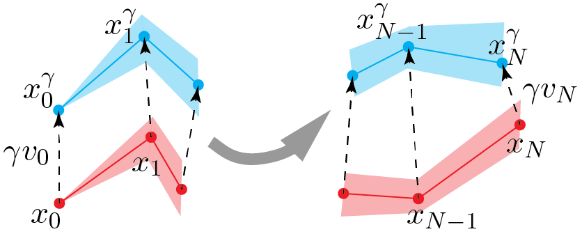
Figure 1. Intuition of the derivative. For different $\gamma$, we compare the blue bundle with the red bundle.

There are three factors in comparing the red bundle with the blue bundle in Figure˜1. The first is $x^{\gamma}_{N}\neq x_{N}$, which induces a difference in $\Phi$. This is given by the path-perturbation, which is the term $d\Phi(x_{N})v_{N}$ in the next subsection.

Then we need to consider that the probability of getting the blue bundle is different from the red bundle. This is given by differentiation on the probability kernel. It is further composed of the second and third factors. The second factor is that the probability density on each path is different. This is the term $\delta p(x^{\gamma}_{n},x^{\gamma}_{n+1})$ in the next subsection.

The third factor is that the corresponding bundles do not occupy the same (Lebesgue) volume. When we specify the expression of $x^{\gamma}_{t}$ from $x_{t}$, we specify the correspondence between a region of $x^{\gamma}_{t}$ and $x_{t}$. These two regions may have different volumes, which contributes to the overall probability they carry. This is the term $\delta J^{\gamma}_{n+1}$ in the next subsection.

How do we decide the correspondence between $x^{\gamma}_{t}$ and $x_{t}$? The first guess would be to quench a background Brownian motion and let $x^{\gamma}_{t}$ and $x_{t}$ be obtained using the same Brownian motion (but different dynamics). This is the pure path-perturbation method. However, it does not work well for unstable systems, where the path-perturbation grows exponentially fast.

The main idea of this paper is that, at each small time step, we ‘divide-and-conquer’ the path-perturbation. That is, when deciding $x^{\gamma}_{n+1}$, we subtract a small portion, $\alpha_{n}v_{n}{\Delta t}$, from the path perturbation, do not let it propagate to the future; instead, we use it to differentiate the kernel. On the other hand, the remaining path-perturbation is propagated to the next step, and some may even hit step $N$ and cause a perturbation in $\Phi(X_{N})$. The tempered path-perturbation gives our rule of pathwise comparison.

Hence, we call our method the ‘path-kernel’ method. The next subsection derives the formula by the ‘divide-and-conquer technique more carefully. In particular, the effect of the portion shifted to kernel-differentiation is given in Equation˜7.

Finally, we remark that our proof can be simplified if we assume that the linear response is linear, that is, the total linear response of many perturbations from different time steps is the sum of the individual responses. If so, using the formula in [23], we can see that the amount shifted at each time step, $\alpha_{n}v_{n}{\Delta t}$, changes the probability density by $\alpha_{n}v_{n}{\Delta B}_{n}/\sigma(x_{n})$, which will affect the density at step $N$. Then we can just sum the response to get the final expression. But linearity in SDE is more worrying than in ODE. The next subsection proves the linearity instead of assuming it, so it is more convincing.

2.3. Derivation

2.3.1. Changing variables

Partition the interval into small segments of length ${\Delta t}$, and the governing equation is Equation˜1. This subsubsection’s main result is Equation˜5, which prescribes the correspondence of paths and associated measures across different $\gamma$. It is obtained after changing the dummy variables from the perturbed path to the unperturbed path.

After partitioning into small time intervals, $\mathbb{E}\left[\Phi(X^{\gamma}_{N})\right]$ has the expression

(2) $$\mathbb{E}\left[\Phi(X^{\gamma}_{N})\right]=\int_{x_{1}}\cdots\int_{x_{N}}\Phi(x^{\gamma}_{N})p(x^{\gamma}_{0},x^{\gamma}_{1})\cdots p(x^{\gamma}_{N-1},x^{\gamma}_{N})dx^{\gamma}_{1}\cdots dx^{\gamma}_{N},$$

where $p(x_{n},x_{n+1})$ is the density of $X_{n+1}$ conditioned on $X_{n}$, it is a Gaussian function with expression

$$p(x^{\gamma}_{n},x^{\gamma}_{n+1})=(2\pi\Delta t)^{-\frac{M}{2}}(\sigma^{\gamma})^{-M}(x^{\gamma}_{n})\exp\left(-\frac{|x^{\gamma}_{n+1}-x^{\gamma}_{n}-F^{\gamma}(x^{\gamma}_{n})\Delta t|^{2}}{2(\sigma^{\gamma})^{2}(x^{\gamma}_{n}){\Delta t}}\right).$$

Sequentially for each $n$, change the variable $x^{\gamma}_{n+1}$ to

$$x_{n+1}^{\gamma}=x_{n+1}+\gamma v_{n+1},$$

where $v_{n}$ is, starting from $v_{0}$, the solution of

(3) $$\begin{split}v_{n+1}=v_{n}-\alpha_{n}v_{n}{\Delta t}+\delta F^{\gamma}(x^{\gamma}_{n}){\Delta t}+\delta\sigma^{\gamma}(x^{\gamma}_{n}){\Delta b}_{n},\quad\textnormal{where}\\ \delta F^{\gamma}(x^{\gamma}_{n}):=\nabla_{v_{n}}F(x_{n})+\delta F^{\gamma}(x_{n}),\\ \delta\sigma^{\gamma}(x^{\gamma}_{n}):=\nabla_{v_{n}}\sigma(x_{n})+\delta\sigma^{\gamma}(x_{n}).\end{split}$$

$\nabla_{v}F(x)$ is the Riemannian derivative of the vector field $F$ along the direction $v$, evaluated at $x$ (note that $v$ must be a vector at $x$).

Note that the dummy variables are the path $\{x_{n}\}_{n=0}^{N}$, not the Brownian increments ${\Delta b}$. At the time we change the variable $x^{\gamma}_{n+1}$ to $x_{n+1}$, $\{x^{\gamma}_{i}\}_{i\leq n}$ have already been changed. In the expression of $v_{n+1}$, only ${\Delta b}_{n}$ depends on $x_{n+1}$, whereas all other terms have been determined by $\{x^{\gamma}_{i}\}_{i\leq n}$. So we still need to denote ${\Delta b}_{n}$ by $x_{n+1}$:

(4) $${\Delta b}_{n}=\frac{1}{\sigma(x_{n})}\left(x_{n+1}-x_{n}-F(x_{n}){\Delta t}\right).$$

Summarizing, the change of variable formula is

$$x_{n+1}^{\gamma}=x_{n+1}\left(1+\frac{\gamma}{\sigma(x_{n})}\delta\sigma^{\gamma}(x^{\gamma}_{n})\right)+\textnormal{terms depend on }x_{0},\ldots,x_{n}.$$

Hence, the Jacobian determinant for the change of variable is

$$\begin{split}J^{\gamma}_{n+1}=\det\frac{\partial x_{n+1}^{\gamma}}{\partial x_{n+1}}=\left(1+\frac{\gamma}{\sigma(x_{n})}\delta\sigma^{\gamma}(x^{\gamma}_{n})\right)^{M}\\ =1+\frac{M\gamma}{\sigma(x_{n})}\delta\sigma^{\gamma}(x^{\gamma}_{n})+\textnormal{high-order terms of }\gamma.\end{split}$$

After changing variables to $x_{n}$’s, Equation˜2 becomes

(5) $$\mathbb{E}\left[\Phi(X^{\gamma}_{N})\right]=\int_{x_{1}}\cdots\int_{x_{N}}\Phi(x^{\gamma}_{N})p(x^{\gamma}_{0},x^{\gamma}_{1})J^{\gamma}_{1}\cdots p(x^{\gamma}_{N-1},x^{\gamma}_{N})J^{\gamma}_{N}dx_{1}\cdots dx_{N},$$

Note that here $x^{\gamma}_{n}$’s and $J^{\gamma}_{n}$’s are functions of $x_{n}$’s. From now on, unless otherwise noted, we only use $x_{n}$’s as the dummy variables when expressing the expectation by multiple integrals.

2.3.2. Taking Derivative

This subsubsection differentiates Equation˜5 with respect to $\gamma$ at $\gamma=0$. This means to compare the path $\{x^{\gamma}_{n}\}_{0\leq n\leq N}$ across different $\gamma$. The main result is

[discrete-time differentiation]

$$\begin{split}\delta\mathbb{E}\left[\Phi(X^{\gamma}_{N})\right]=\mathbb{E}\left[d\Phi(X_{N})v_{N}+\Phi(X_{N})\sum_{n=0}^{N-1}\frac{{\Delta B}_{n}}{\sigma(X_{n})}\cdot\alpha_{n}v_{n}.\right]\end{split}$$

Proof.

Note that $J_{n}=1$ for $\gamma=0$. Differentiate Equation˜5 at $\gamma=0$ and apply the Leibniz rule, we get

(6) $$\delta\mathbb{E}\left[\Phi(X^{\gamma}_{N})\right]=\mathbb{E}\left[\delta\Phi(X^{\gamma}_{N})\right]+\sum_{n=0}^{N-1}\mathbb{E}\left[\Phi(X_{N})\left(\frac{\delta p(X^{\gamma}_{n},X^{\gamma}_{n+1})}{p(X_{n},X_{n+1})}+\delta J^{\gamma}_{n+1}\right)\right].$$

We compute each of these terms. For the first term, since $\gamma=0$,

$$\delta\Phi(X^{\gamma}_{N})=d\Phi\,\delta X_{N}=d\Phi\,v_{N}.$$

Here $d\Phi$ is the differential of $\Phi$.

For the second term,

$$\frac{\delta p(X^{\gamma}_{n},X^{\gamma}_{n+1})}{p(X_{n},X_{n+1})}=-M\frac{\delta\sigma^{\gamma}(X^{\gamma}_{n})}{\sigma(X_{n})}-\frac{{\Delta B}_{n}\cdot(v_{n+1}-v_{n}-\delta F^{\gamma}(X^{\gamma}_{n})\Delta t)}{\sigma(X_{n}){\Delta t}}+\frac{{\Delta B}_{n}^{2}\,\delta\sigma^{\gamma}(X^{\gamma}_{n})}{\sigma(X_{n}){\Delta t}}$$

Here ${\Delta B}_{n}$ is a function of $X_{n}$ and $X_{n+1}$, whose expression is in Equation˜4, $v_{n}$ is a function of $\{X_{i}\}_{0\leq i\leq n}$, and ${\Delta B}^{2}:={\Delta B}\cdot{\Delta B}$.

For the third term,

$$\begin{split}\delta J^{\gamma}_{n+1}=\frac{M}{\sigma(X_{n})}\delta\sigma^{\gamma}(X^{\gamma}_{n}).\end{split}$$

The summand in Equation˜6, the second and third term, is the perturbation applied on the probability kernel at each step. After cancellation,

(7) $$\begin{split}\frac{\delta p(X^{\gamma}_{n},X^{\gamma}_{n+1})}{p(X_{n},X_{n+1})}+\delta J^{\gamma}_{n+1}=-\frac{{\Delta B}_{n}}{\sigma(X_{n}){\Delta t}}\cdot(v_{n+1}-v_{n}-\delta F^{\gamma}(X^{\gamma}_{n}){\Delta t}-\delta\sigma^{\gamma}(X^{\gamma}_{n}){\Delta B}_{n}).\end{split}$$

By the definition of $v_{n}$ in Equation˜3,

$$\begin{split}\frac{\delta p(X^{\gamma}_{n},X^{\gamma}_{n+1})}{p(X_{n},X_{n+1})}+\delta J^{\gamma}_{n+1}=\frac{{\Delta B}_{n}}{\sigma(X_{n}){\Delta t}}\cdot\alpha_{n}v_{n}{\Delta t}=\frac{{\Delta B}_{n}}{\sigma(X_{n})}\cdot\alpha_{n}v_{n}.\end{split}$$

For the pure path-perturbation method, $\alpha\equiv 0$, and the above is zero since nothing hits the kernel. But we choose to shift a small portion of the path-perturbation, proportional to $\alpha{\Delta t}$, and use that to differentiate the kernel.

Putting everything together, we get the expression in the lemma. ∎

2.3.3. Continuous-time and ergodic statements

So far, our proof on discrete-time is rigorous. Now, without rigorous proof and without worrying about regularities, we formally let ${\Delta t}\rightarrow 0$ and present continuous-time statements. We also provide a single-path formula for physical measures.

See 1.2

Note that changing $\Phi$ by adding a constant does not affect the linear response. So we can freely subtract $\Phi^{avg}_{T}:=\mathbb{E}\left[\Phi(X^{\gamma}_{T})\right]$, and the following is still correct. This formula is better for numerical purposes, since the integrand in the average is smaller after ‘centralization’, or subtracting $\Phi^{avg}_{T}$. [centralized path-kernel formula]

$$\delta\mathbb{E}\left[\Phi(X^{\gamma}_{T})\right]=\mathbb{E}\left[d\Phi(X_{T})v_{T}+(\Phi(X_{T})-\Phi^{avg}_{T})\int_{t=0}^{T}\frac{\alpha_{t}v_{t}}{\sigma(x_{t})}\cdot dB.\right]$$

For the case of the physical measure, we can formally substitute $T=\infty$, to get

$$\delta\mathbb{E}_{\mu^{\gamma}}\left[\Phi(X)\right]=\lim_{T\rightarrow\infty}\mathbb{E}\left[d\Phi(X_{T})v_{T}\right]+\int_{t=0}^{T}\mathbb{E}\left[(\Phi(X_{T})-\Phi^{avg})\,\frac{\alpha_{t}v_{t}}{\sigma(x_{t})}\cdot dB_{t}\right],$$

where $\Phi^{avg}:=\mathbb{E}_{\mu}\left[\Phi(X)\right]$. In this expression, $T$ is both the orbit length and the decorrelation length. We assume decay of correlations, that is, for smooth observables $f$ and $g$

$$\mathbb{E}_{\mu}\left[f(X_{s})g(X_{t})\right]\rightarrow\mathbb{E}_{\mu}\left[f(X)\right]\mathbb{E}_{\mu}\left[g(X)\right]$$

very fast as $|t-s|\rightarrow\infty$. Since we are using Ito integration, $\mathbb{E}\left[\frac{\alpha_{t}v_{t}}{\sigma(x_{t})}\cdot dB_{t}\right]=0$. So we have the convergence of the time-integral. Using $W$ and $T$ to indicate the decorrelation and orbit length separately, we have

$$\delta\mathbb{E}_{\mu^{\gamma}}\left[\Phi(X)\right]=\mathbb{E}_{\mu}\left[d\Phi(X)v\right]+\lim_{W\rightarrow\infty}\int_{\tau=0}^{W}\mathbb{E}_{\mu}\left[(\Phi(X_{W})-\Phi^{avg})\,\frac{\alpha_{\tau}v_{\tau}}{\sigma(x_{\tau})}\cdot dB_{\tau}\right],$$

We can compute it by averaging along a single orbit using the formula below, where, typically, $W\ll T$ in numerics. [ergodic path-kernel formula]

$$\begin{split}\delta\mathbb{E}\left[\Phi(X^{\gamma})\right]\,\overset{\mathrm{a.s.}}{=}\,\lim_{W\rightarrow\infty}\lim_{T\rightarrow\infty}\frac{1}{T}\int_{t=0}^{T}\left[d\Phi(X_{t})v_{t}+\left(\Phi(X_{t+W})-\Phi^{avg}\right)\int_{\tau=0}^{W}\frac{\alpha_{t+\tau}v_{t+\tau}}{\sigma(x_{t+\tau})}\cdot dB_{t+\tau}\right].\end{split}$$

2.4. How to use in unstable cases, and shortcomings

We explain how to use this formula in chaotic random dynamics, in particular, how to select the schedule $\alpha_{t}$. Then we explain the shortcomings of the method. Note that $v_{t}$ depends on $\alpha_{t}$, but any choice of $\alpha_{t}$ yields the same $\delta\mathbb{E}\left[\Phi(X^{\gamma}_{T})\right]$. The different choices of $\alpha_{t}$ significantly affect the numerical performances.

Assume that the largest Lyapunov exponent is $\lambda$. More specifically, let $f_{*}^{t}$ be the operator such that $f_{*}^{t}v_{0}$ solves the homogeneous ODE,

$$\begin{split}du=\nabla_{u}F(X)dt+d\sigma(X)udB\end{split}$$

from the initial condition $v_{0}$. Then we define $\lambda$ as

$$\begin{split}\lambda:=\frac{1}{T}\log|f_{*}^{T}|,\end{split}$$

where $|f_{*}^{T}|$ is the operator norm. For physical measures, we let $T\rightarrow\infty$.

We say that the dynamic is unstable or chaotic if $\lambda>0$. For this case, to use the path-kernel formula, we can set

$$\begin{split}\alpha_{t}\equiv\alpha>\lambda.\end{split}$$

If so, then the solution of

$$\begin{split}dv=-\alpha vdt+\nabla_{v}F(X)dt+d\sigma(X)vdB\end{split}$$

is $e^{-\alpha t}u$. Hence, the homogeneous solution does not grow with time, and we control the size of the integrand in the linear response formula. In correspondence, the linear response now has the extra term involving $\alpha_{t}$, due to differentiating the probability kernel. We say that the chaotic behavior has been tempered by shifting the path-perturbation to kernel-differentiation.

Should we care very much about the numerical speed, we should design $\alpha_{t}$ more carefully. Note that $\alpha_{t}$ can be a process, not just a fixed number. If the system has regions with large unstableness, then $\alpha_{t}$ should be large there to reduce the growth of $v_{t}$. If the system has regions with small noise, then $\alpha_{t}$ should be small, since the $1/\sigma$ factor is already large. The path-kernel formula would yield the same derivative, but an adapted $\alpha_{t}$ gives a smaller integrand, so we need fewer samples. In this paper, we only test the simple case where $\alpha_{t}$ is a fixed number.

Our path-kernel method combines the path-perturbation and kernel-differentiation methods, but does not involve the divergence method. Hence, it does not work in highly unstable systems with little to no noise, the case where the divergence method is good. Since the system is unstable, we need a large $\alpha$ to tame the gradient explosion, but the noise is small, so the $\frac{1}{\sigma}$ factor is large. This requires many samples to compute the expectation, drastically raising the computational cost. The divergence method is not a panacea either; it does not work when there are contracting directions. Eventually, we may need to use all three methods together for an ultimate solution.

3. Degeneration to some well-known cases

3.1. Degeneracy to pure path-perturbation

Consider the special case where we set

$$\begin{split}\alpha_{t}\equiv 0.\end{split}$$

So we are not transferring any path-perturbation to the probability kernel. Hence, $v_{t}$ degenerates to $u_{t}$, the solution of the (undamped) path-perturbation equation

$$du=\left(\nabla_{u}F(X)+\delta F^{\gamma}(X)\right)dt+\left(d\sigma(X)u+\delta\sigma^{\gamma}(X)\right)dB.$$

This is the governing equation for the path-perturbation due to changing $\gamma$, under a quenched Brownian motion. And our linear response formula degenerates to

$$\delta\mathbb{E}\left[\Phi(X^{\gamma}_{T})\right]=\mathbb{E}\left[d\Phi(X_{T})u_{T}\right].$$

This is the pure path-perturbation formula. Intuitively, for each Brownian motion, the SDE becomes an ODE, and we consider how the path of the ODE changes due to changing $\gamma$. Then we compute how this path-perturbation affects the value of $\Phi$ at time $T$ by $d\Phi(X_{T})u_{T}$.

When the path-perturbation is unstable, $u_{t}$ grows exponentially fast and the integrand becomes too large. Computing the expectation requires taking too many samples. In contrast, the schedule function $\alpha_{t}$ in our path-kernel formula allows a damping factor on $v_{t}$, which tempers the gradient explosion.

3.2. Degeneracy to pure kernel-differentiation

Consider the special case where $\sigma^{\gamma}(x)$ is a constant $C$ independent of $x$ and $\gamma$. In correspondence, in the discrete-time derivation, we set

$$\begin{split}\alpha_{n}\equiv\frac{1}{{\Delta t}}.\end{split}$$

Consequently, the governing equation of $v_{n}$, Equation˜3, becomes

$$\begin{split}v_{n+1}=\delta F^{\gamma}(X^{\gamma}_{n}){\Delta t},\quad\textnormal{where}\quad\delta F^{\gamma}(X^{\gamma}_{n}):=\nabla_{v_{n}}F(X_{n})+\delta F^{\gamma}(X_{n}).\end{split}$$

Intuitively, the perturbation on dynamic generated at the current time step, $\delta F^{\gamma}(x^{\gamma}_{n}){\Delta t}$, is small, so we can throw it entirely to the kernel, let it differentiate the kernel, and do not let any portion propagate: hence it gets the name ‘kernel-differentiation method.

Note that $v_{n}$ is $O({\Delta t})$, so the ${\Delta t}$’s cancel in $\alpha_{n}v_{n}$, and Section˜2.3.2 becomes

$$\begin{split}\delta\mathbb{E}\left[\Phi(X^{\gamma}_{T})\right]=\mathbb{E}\left[d\Phi(X_{N})v_{N}+\Phi(X_{N})\sum_{n=0}^{N-1}\frac{{\Delta B}_{n}}{\sigma(X_{n})}\cdot\alpha_{n}v_{n}\right]\\ =\mathbb{E}\left[d\Phi(X_{N})\delta F^{\gamma}(X^{\gamma}_{N-1}){\Delta t}+\Phi(X_{N})\sum_{n=0}^{N-1}\frac{{\Delta B}_{n}}{\sigma(X_{n})}\cdot\delta F^{\gamma}(X^{\gamma}_{n})\right]\\ =\mathbb{E}\left[d\Phi(X_{N})\delta F^{\gamma}(X^{\gamma}_{N-1}){\Delta t}+\Phi(X_{N})\sum_{n=0}^{N-1}\frac{{\Delta B}_{n}}{\sigma(X_{n})}\cdot\left(\nabla_{v_{n}}F(X_{n})+\delta F^{\gamma}(X_{n})\right)\right]\end{split}$$

As ${\Delta t}\rightarrow 0$, the first term goes to zero. The second term is the sum of the $O({\Delta t}{\Delta B})$ terms, so it also goes to zero. Hence, the continuous-time expression is

$$\begin{split}\delta\mathbb{E}\left[\Phi(X^{\gamma}_{N})\right]=\mathbb{E}\left[\Phi(X_{T})\int_{t=0}^{T}\frac{\delta F^{\gamma}(X_{n})}{\sigma(X_{n})}\cdot dB\right].\end{split}$$

For the general case where $\sigma^{\gamma}(x)$ is not a constant, this pure kernel-differentiation method, or this choice of schedule $\alpha_{n}$ does not work, since the portion shifted to the kernel, $\alpha_{n}v_{n}{\Delta t}$, is too large. Here $v_{n}$ becomes $O({\Delta B})$, but $\alpha_{n}$ is $O(1/{\Delta t})$: this is to be illustrated in the example in Section˜3.3. When substituting into Section˜2.3.2, $\alpha_{n}v_{n}$ is $O({\Delta B}/{\Delta t})$, so the expression of $\delta\mathbb{E}\left[\Phi(X^{\gamma}_{N})\right]$ becomes a sum of $O(1)$ terms, which converges poorly as ${\Delta t}\rightarrow 0$. In numerics, this means that the pure kernel-differentiation method requires many samples to compute the expectation. This should be why the pure kernel-differentiation method could not consider perturbations on the diffusion term. But it has a simpler and more intuitive derivation on this degenerate case via transfer operators [23].

3.3. Degeneracy to a big Gaussian

We use this case to illustrate why the path-perturbation method could help the pure kernel-differentiation method for perturbations on diffusion: this is why we combine the two. Consider the special case where $F(\cdot)\equiv 0$, $x_{0}=0$, $v_{0}=0$, and $\sigma^{\gamma}(x)=1+\gamma$ which is independent of $x$. The SDE becomes $dX_{t}^{\gamma}=(1+\gamma)dB$, so the solution is

$$\begin{split}X^{\gamma}_{t}=(1+\gamma)B_{t}.\end{split}$$

In particular,

$$\begin{split}X^{\gamma}_{T}=(1+\gamma)\sum_{n=0}^{N}{\Delta B}_{n}.\end{split}$$

First, for the pure kernel method, in the discrete-time derivation, set

$$\begin{split}\alpha_{n}\equiv\frac{1}{{\Delta t}}.\end{split}$$

Consequently, the governing equation of $v_{n}$, Equation˜3, becomes

$$\begin{split}v_{n+1}={\Delta B}_{n},\quad v_{0}=0.\end{split}$$

By Section˜2.3.2, the linear response is pure kernel-differentiation

(8) $$\begin{split}\delta\mathbb{E}\left[\Phi(X^{\gamma}_{T})\right]=\mathbb{E}\left[d\Phi(X){\Delta B}_{N-1}\right]+\mathbb{E}\left[\Phi(X_{N})\sum_{n=1}^{N-1}\frac{{\Delta B}_{n}\cdot{\Delta B}_{n-1}}{{\Delta t}}\right].\end{split}$$

If we were to numerically compute it, we are summing $N$-many $O(1)$ terms, so we would get a large sum, which takes many sample paths to average. So it fails.

On the other hand, if we set

$$\begin{split}\alpha_{t}\equiv 0.\end{split}$$

Then $v_{n+1}=v_{n}+{\Delta B}_{n}$, hence

$$\begin{split}v_{N}=B_{N}.\end{split}$$

The linear response is now

$$\begin{split}\delta\mathbb{E}\left[\Phi(X^{\gamma}_{N})\right]=\mathbb{E}\left[d\Phi(X_{N})B_{N}\right]\end{split}$$

This is the pure path-perturbation formula.

Intuitively, if we do not immediately let the perturbation from dynamics hit the kernel, but let it propagate along the path for some time, then the ${\Delta B}$ terms in the perturbations on dynamics from different time steps cancel, and the path-perturbation remains bounded. This prevents the integrand from becoming too large. In our path-kernel method, we let most of the perturbation propagate, and only use a small portion to differentiate the kernel in each step. So, the ${\Delta B}$ terms also mostly cancel.

Alerted readers may question whether the two linear response formulas we obtained with two extreme schedule functions are equivalent. They are equivalent formulas with very different performances in analysis and numerics. To see the equivalence, in Equation˜8, use the Brownian increment as the dummy variable, whose density is

$$\begin{split}p({\Delta b})=(2\pi\Delta t)^{-\frac{M}{2}}\exp\left(-\frac{|{\Delta b}|^{2}}{2{\Delta t}}\right).\end{split}$$

So its differential is

$$\begin{split}dp({\Delta b})=-\frac{{\Delta b}}{{\Delta t}}\,p({\Delta b})\end{split}$$

Move integrations on ${\Delta b}_{n}$ to the first place, the main term in Equation˜8 becomes

$$\begin{split}&\mathbb{E}\left[\frac{\Phi(X_{N})}{{\Delta t}}{\Delta B}_{n}\cdot{\Delta B}_{n-1}\right]\\ =&\int_{{\Delta b}_{0}}\cdots\int_{{\Delta b}_{N-1}}\Phi(x_{N})\frac{{\Delta b}_{n}\cdot{\Delta b}_{n-1}}{{\Delta t}}\,p({\Delta b}_{N-1})d{\Delta b}_{N-1}\cdots p({\Delta b}_{0})d{\Delta b}_{0}\\ =&-\int\cdots\int_{{\Delta b}_{N-1}}\left(\int_{{\Delta b}_{n}}\Phi(x_{N})dp({\Delta b}_{n})d{\Delta b}_{n}\right){\Delta b}_{n-1}p({\Delta b}_{N-1})d{\Delta b}_{N-1}\cdots\end{split}$$

Integrate by parts on ${\Delta b}_{n}$, note that $\Phi(x_{N})=\Phi({\Delta b}_{0}+\cdots+{\Delta b}_{N-1})$, so $\partial\Phi(x_{n})/\partial{\Delta b}_{n}=d\Phi(x_{N})$. Hence,

$$\begin{split}=&\int\cdots\int_{{\Delta b}_{N-1}}\left(\int_{{\Delta b}_{n}}d\Phi(X_{N})p({\Delta b}_{n})d{\Delta b}_{n}\right){\Delta b}_{n-1}p({\Delta b}_{N-1})d{\Delta b}_{N-1}\cdots\\ =&\,\mathbb{E}\left[d\Phi(X_{N}){\Delta B}_{n-1}\right].\end{split}$$

So Equation˜8 becomes

$$\begin{split}\delta\mathbb{E}\left[\Phi(X^{\gamma}_{T})\right]=\mathbb{E}\left[d\Phi(X){\Delta B}_{N-1}\right]+\sum_{n=1}^{N-1}\mathbb{E}\left[d\Phi(X_{N}){\Delta B}_{n-1}\right]=\mathbb{E}\left[d\Phi(X_{N})B_{N}\right],\end{split}$$

which equals the pure path-perturbation formula.

3.4. Degeneracy to Bismut-Elworthy-Li formula

We use this case to show two main differences from the Bismut-Elworthy-Li formula. The first is that our path-kernel method allows $F$ and $\sigma$ to depend on $\gamma$. The second is that our schedule function tempers the unstableness better.

Consider the special case where $F(x)$ and $\sigma(x)$ do not depend on $\gamma$, and only $X^{\gamma}_{0}=x_{0}+\gamma v_{0}$ depends on $\gamma$. To get the Bismut-Elworthy-Li formula, first let $u$ be the pure path-perturbation

$$du=\nabla_{u}F(X)dt+d\sigma(X)udB,\quad u_{0}=v_{0}.$$

And let $\beta_{t}=(T-t)/T$.

In our notation, we let $v=\beta_{t}u$, so $v$ is the solution of

$$\begin{split}dv=\frac{d\beta_{t}}{dt}udt+\beta_{t}u=\frac{d\beta_{t}}{\beta_{t}dt}\beta_{t}udt+\nabla_{\beta_{t}u}F(X)dt+(d\sigma(X)\beta_{t}u)dB\\ =-\frac{1}{T-t}vdt+\nabla_{v}F(X)dt+(d\sigma(X)v)dB,\end{split}$$

from the given initial condition $v_{0}$. So our schedule function is

$$\begin{split}\alpha_{t}=\frac{1}{T-t}.\end{split}$$

Hence, $\alpha_{t}v_{t}=\alpha_{t}\beta_{t}u_{t}=u_{t}/T$. Also note that $v_{T}=0$ by definition of $v$.

With these, our main theorem degenerates to the following expression, which is the Bismut-Elworthy-Li formula.

$$\delta\mathbb{E}\left[\Phi(X^{\gamma}_{T})\right]=\mathbb{E}\left[\Phi(X_{T})\int_{t=0}^{T}\frac{\alpha_{t}v_{t}}{\sigma(X_{t})}\cdot dB\right]=\frac{1}{T}\mathbb{E}\left[\Phi(X_{T})\int_{t=0}^{T}\frac{u_{t}}{\sigma(X_{t})}\cdot dB\right].$$

The benefit is that we do not need the differentiability of $\Phi$ since $v_{T}=0$.

The downside of using the special schedule is that it tends to damp the instability unevenly: it incurs too little damping at the start of the time span. $u_{t}$ can grow too large and it requires many samples to compute the expectation. In contrast, we choose $\alpha_{t}$ to act in a way such that it reduces the growth rate of $v_{t}$ uniformly. This contrast is even sharper when we compute the linear response of physical measures, since $u_{t}$ can grow unbounded over an infinite time span in a unstable system.

4. Algorithm and numerical examples

This section gives the procedure list of the algorithm and demonstrates the algorithm on an example. Here, $\delta$ can be the derivative evaluated at $\gamma\neq 0$; the dependence on $\gamma$ should be clear from context.

4.1. Procedure lists

First, we give Algorithm˜1 for the finite-time system. We use the Euler scheme to integrate SDEs, which coincides with our discrete-time formulation in Section˜2.3.2.

Algorithm 1 Path-kernel algorithm on finite time span $[0,T]$

number of sample paths $L$, ${\Delta t}$, $N=T/{\Delta t}$, $v_{0}$.

for $l=1,\dots,L$ do

  Set $x_{0}$ as given, or independently generate sample $x_{0}$.

  for $n=0,\dots,N-1$ do

   Independently generate sample ${\Delta b}_{n}$ from $N(0,{\Delta t})$

   $\alpha_{n}\leftarrow\alpha_{n{\Delta t}}$, which could depend on $\{x_{i}\}_{i\leq n}$

   $I_{n}\leftarrow\frac{{\Delta b}_{n}}{\sigma(x_{n})}\cdot\alpha_{n}v_{n}$

   $x_{n+1}\leftarrow x_{n}+F(x_{n}){\Delta t}+\sigma(x_{n}){\Delta b}_{n}$

   $v_{n+1}\leftarrow v_{n}-\alpha_{n}v_{n}{\Delta t}+\left(\nabla_{v_{n}}F+\delta F^{\gamma}\right)(x_{n}){\Delta t}+\left(d\sigma v_{n}+\delta\sigma^{\gamma}\right)(x_{n}){\Delta b}_{n}$

  end for

  $\Phi_{l}\leftarrow\Phi(x_{N})$

  $S^{1}_{l}\leftarrow d\Phi(x_{N})v_{N}$

  $S^{2}_{l}\leftarrow\sum_{n=0}^{N-1}I_{n}$ $\triangleright$ No need to store entire path.

end for

$\Phi_{T}^{avg}\approx\frac{1}{L}\sum_{l=1}^{L}\Phi_{l}$

$\delta\mathbb{E}\left[\Phi(X^{\gamma}_{T})\right]\approx\frac{1}{L}\sum_{l=1}^{L}\left(S^{1}_{l}+\left(\Phi_{l}-\Phi_{T}^{avg}\right)S^{2}_{l}\right)$

Then we give Algorithm˜2 for the infinite-time case. Here $M_{pre}$ is the number of preparation steps, during which $x_{0}$ lands onto the physical measure. Here $W$ is the decorrelation time length, $T$ is the orbit length, typically $W\ll T$.

Algorithm 2 Path-kernel algorithm for physical measure on infinite time span

$M_{pre},{\Delta t},N_{W}=W/{\Delta t},N=T/{\Delta t}$.

Take any $x_{0}$ or $v_{0}$.

for $n=0,\cdots,M_{pre}$ do

  Independently generate sample ${\Delta b}$ from $N(0,{\Delta t})$

  $x_{0}\leftarrow x_{0}+F(x_{0}){\Delta t}+\sigma(x_{0}){\Delta b}$

end for

for $n=0,\cdots,N_{W}+N-1$ do

  Compute ${\Delta b}_{n},\alpha_{n},I_{n},x_{n+1},v_{n+1}$ as above

  $\Phi_{n}\leftarrow\Phi(x_{n})$

  $S^{1}_{n}\leftarrow d\Phi(x_{n})v_{n}$

  If $n\geq N_{W}$, $S^{2}_{n}\leftarrow\sum_{m=0}^{N_{W}-1}I_{n+m-N_{W}}$

end for

$\Phi^{avg}\approx\frac{1}{N}\sum_{n=N_{W}}^{N_{W}+N-1}\Phi_{n}$

$\delta\Phi^{avg}\approx\frac{1}{N}\sum_{n=N_{W}}^{N_{W}+N-1}\left(S^{1}_{n}+\left(\Phi_{n}-\Phi^{avg}\right)S^{2}_{n}\right)$

From a utility point of view, the current version of the path-kernel method is not an ‘adjoint’ algorithm. So its cost is proportional to the dimension of $\gamma$. But an adjoint version is straightforward. Note that $v$ is the result of applying a linear operator on the non-homogeneous term $\delta F^{\gamma}(X)dt+\delta\sigma^{\gamma}(X)dB$. To get the adjoint formula, we just need to move the linear operator to $\frac{\alpha}{\sigma}dB$ by the standard technique.

4.2. Numerical example: Lorenz 96 with noise

We demonstrate our algorithm over the Lorenz 96 model [18], with additive noise in $\mathbb{R}^{M}$, where the dimension of the system is $M=40$. The SDE is

$$\begin{split}dX^{i}=\left(\left(X^{i+1}-X^{i-2}\right)X^{i-1}-X^{i}+8+\gamma^{0}-0.01(X^{i})^{2}\right)dt+(1+\gamma^{1})\sigma_{0}dB^{i}\\ \textnormal{for }i=1,\ldots,M;\quad X^{\gamma}_{0}=\gamma^{2}[1,\ldots,1].\end{split}$$

Here it is assumed that $X^{-1}=X^{M-1},X^{0}=X^{M}$ and $X^{M+1}=x^{1}$, where $x^{i}$ is the state of the system. $\gamma^{0},\gamma^{1},\gamma^{2}$ are three parameters that control the drift term, the diffusion term, and the initial condition. We added noise and the $-0.01(X^{i})^{2}$ term, which prevents the noise from carrying us to infinitely far away. The observable function $\Phi$ is set as

$$\begin{split}\Phi(x):=\frac{1}{M}\sum_{i=1}^{M}x^{i}.\end{split}$$

We set $\sigma_{0}=0.5$, a relatively small noise.

No previous linear response methods work for this problem. This problem is unstable, so pure path-perturbation does not work. The diffusion coefficient is controlled by the parameters, so pure kernel-differentiation does not work. The dynamics is controlled by the parameters, and we also consider linear response of physical measures, so Bismut-Elworthy-Li does not work for either case. The system is non-hyperbolic, so the fast response method does not work.

First, we compute the parameter-derivatives of $\Phi^{avg}_{T}:=\mathbb{E}\left[\Phi(X_{T})\right]$ for $T=1$. A typical orbit is in Figure˜2. In our algorithm, we set ${\Delta t}=0.002$, and

$$\begin{split}\alpha_{t}\equiv 10.\end{split}$$

So, all unstableness are tempered. The default values of all $\gamma^{i}$’s are zero. We compute the derivative with respect to $\gamma^{1}$ controlling the noise level, $\gamma^{0}$ controlling the drift term, and $\gamma^{2}$ controlling the initial condition. The results are shown in Figures˜3 and 4; the derivative computed by the path-kernel method is correct.

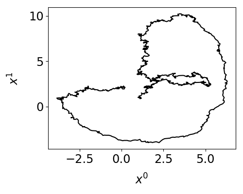
Figure 2. Plot of $x^{0}_{t},x^{1}_{t}$ from a typical orbit of length $T=2$.

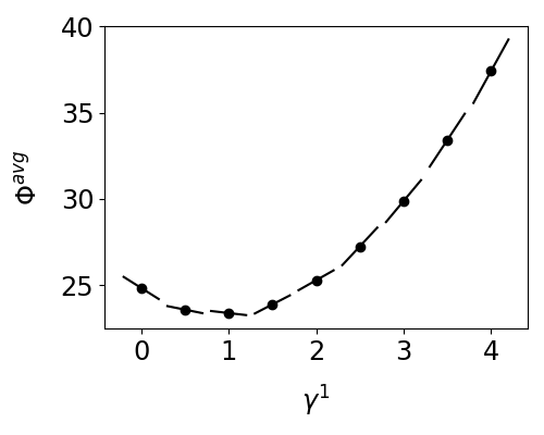
Figure 3. $\Phi^{avg}_{T}$ and $\delta\Phi^{avg}_{T}$ for different $\gamma^{1}$. The dots are $\Phi^{avg}_{T}$, and the short lines are $\delta\Phi^{avg}_{T}$ computed by the kernel-differentiation algorithm; they are computed from the same orbit.

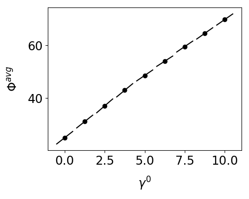
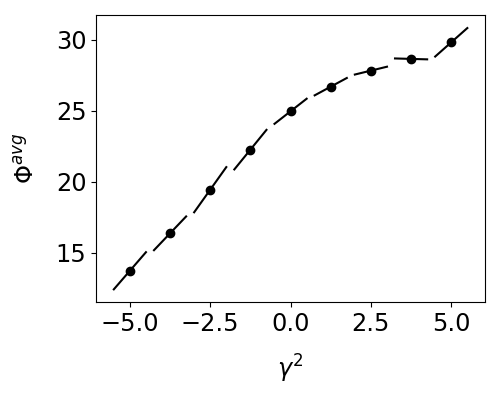
Figure 4. $\Phi^{avg}_{T}$ and $\delta\Phi^{avg}_{T}$ for different $\gamma^{0}$ and $\gamma^{2}$.

Then we compute the linear response to $\gamma^{0}$ for the physical measure. In Algorithm˜2, we set $T=1000$ and $W=1$. The results are in Figure˜5. As we can see, the algorithm gives an accurate linear response for the noised case. Moreover, the linear response of $\gamma^{0}$ in the noised case is a reasonable reflection of the observable-parameter relation in the deterministic case.

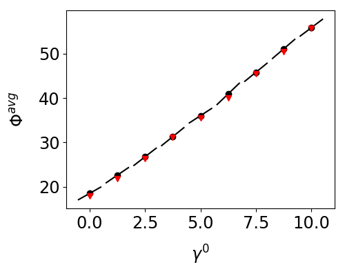
Figure 5. $\Phi^{avg}$ and $\delta\Phi^{avg}$ of the physical measure for different $\gamma^{0}$. The red triangles are $\Phi^{avg}$ for the Lorenz 96 system without noise.

We also compute the linear response to $\gamma^{1}$ for the physical measure, and compare with the pure kernel-differentiation method. By Section˜3.2, the pure kernel-differentiation can be obtained by setting $\alpha\equiv 1/{\Delta t}$ in the path-kernel formula. We keep all other settings the same. Figure˜6 shows that our path-kernel method performs much better than the pure kernel method. We also tried the pure path-perturbation method; it overflows halfway, so there is nothing to compare with.

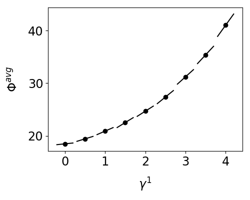
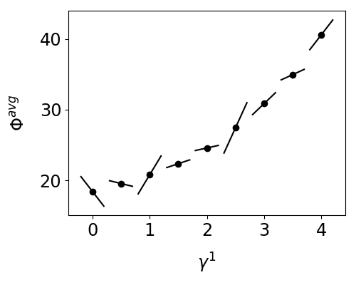
Figure 6. $\Phi^{avg}$ and $\delta\Phi^{avg}$ of the physical measure for different $\gamma^{1}$. Left: the derivatives are computed by path-kernel method. Right: the derivatives are computed by pure kernel method.

Data availability statement

The code used in this paper is posted at https://github.com/niangxiu/paker. There are no other associated data.

References

- [1] W. Bahsoun, M. Ruziboev, and B. Saussol. Linear response for random dynamical systems. Advances in Mathematics, 364:107011, 4 2020.
- [2] V. Baladi. The quest for the ultimate anisotropic Banach space. Journal of Statistical Physics, 166:525–557, 2017.
- [3] J.-M. Bismut. Large Deviations and the Malliavin Calculus, volume 45. Birkhäuser Boston Inc., Progress in Mathematics, 1984.
- [4] R. Bowen and D. Ruelle. The ergodic theory of axiom A flows. Inventiones Mathematicae, 29:181–202, 1975.
- [5] D. Dolgopyat. On differentiability of SRB states for partially hyperbolic systems. Inventiones Mathematicae, 155:389–449, 2004.
- [6] D. Dragičević, P. Giulietti, and J. Sedro. Quenched linear response for smooth expanding on average cocycles. Communications in Mathematical Physics, 399:423–452, 4 2023.
- [7] R. Durrett. Probability: Theory and Examples. Cambridge University Press, 4th edition edition, 8 2010.
- [8] K. Elworthy and X. Li. Formulae for the derivatives of heat semigroups. Journal of Functional Analysis, 125:252–286, 10 1994.
- [9] G. L. Eyink, T. W. N. Haine, and D. J. Lea. Ruelle’s linear response formula, ensemble adjoint schemes and lévy flights. Nonlinearity, 17:1867–1889, 2004.
- [10] S. Galatolo and P. Giulietti. A linear response for dynamical systems with additive noise. Nonlinearity, 32:2269–2301, 6 2019.
- [11] S. Galatolo and A. Ni. Optimal response for hyperbolic systems by the fast adjoint response method. arXiv:2501.02395, 1 2025.
- [12] S. Galatolo and I. Nisoli. An elementary approach to rigorous approximation of invariant measures. SIAM Journal on Applied Dynamical Systems, 13:958–985, 2014.
- [13] S. Galatolo and M. Pollicott. Controlling the statistical properties of expanding maps. Nonlinearity, 30:2737–2751, 7 2017.
- [14] P. W. Glynn. Likelihood ratio gradient estimation for stochastic systems. Communications of the ACM, 33:75–84, 10 1990.
- [15] S. Gouëzel and C. Liverani. Compact locally maximal hyperbolic sets for smooth maps: Fine statistical properties. Journal of Differential Geometry, 79:433–477, 2008.
- [16] M. Hairer and A. J. Majda. A simple framework to justify linear response theory. Nonlinearity, 23:909–922, 4 2010.
- [17] M. Jiang. Differentiating potential functions of SRB measures on hyperbolic attractors. Ergodic Theory and Dynamical Systems, 32:1350–1369, 2012.
- [18] E. N. Lorenz. Predictability – a problem partly solved, pages 40–58. Cambridge University Press, 7 2006.
- [19] V. Lucarini, F. Ragone, and F. Lunkeit. Predicting climate change using response theory: Global averages and spatial patterns. Journal of Statistical Physics, 166:1036–1064, 2017.
- [20] A. Ni. Fast linear response algorithm for differentiating chaos. arXiv:2009.00595, pages 1–28, 2020.
- [21] A. Ni. Fast adjoint algorithm for linear responses of hyperbolic chaos. SIAM Journal on Applied Dynamical Systems, 22:2792–2824, 12 2023.
- [22] A. Ni. Backpropagation in hyperbolic chaos via adjoint shadowing. Nonlinearity, 37:035009, 3 2024.
- [23] A. Ni. Ergodic and foliated kernel-differentiation method for linear responses of random systems. arXiv:2410.10138, 10 2024.
- [24] A. Ni and C. Talnikar. Adjoint sensitivity analysis on chaotic dynamical systems by non-intrusive least squares adjoint shadowing (NILSAS). Journal of Computational Physics, 395:690–709, 2019.
- [25] A. Ni and Y. Tong. Recursive divergence formulas for perturbing unstable transfer operators and physical measures. Journal of Statistical Physics, 190:126, 7 2023.
- [26] A. Ni and Y. Tong. Equivariant divergence formula for hyperbolic chaotic flows. Journal of Statistical Physics, 191:118, 9 2024.
- [27] P. Plecháč, G. Stoltz, and T. Wang. Martingale product estimators for sensitivity analysis in computational statistical physics. IMA Journal of Numerical Analysis, 43:3430–3477, 11 2023.
- [28] M. I. Reiman and A. Weiss. Sensitivity analysis for simulations via likelihood ratios. Operations Research, 37:830–844, 10 1989.
- [29] P. Ren and F.-Y. Wang. Bismut formula for lions derivative of distribution dependent sdes and applications. Journal of Differential Equations, 267:4745–4777, 10 2019.
- [30] R. Y. Rubinstein. Sensitivity analysis and performance extrapolation for computer simulation models. Operations Research, 37:72–81, 2 1989.
- [31] D. Ruelle. A measure associated with axiom-A attractors. American Journal of Mathematics, 98:619, 1976.
- [32] D. Ruelle. Differentiation of SRB states. Commun. Math. Phys, 187:227–241, 1997.
- [33] C. Wormell. Spectral Galerkin methods for transfer operators in uniformly expanding dynamics. Numerische Mathematik, 142:421–463, 2019.
- [34] L.-S. Young. What are SRB measures, and which dynamical systems have them? Journal of Statistical Physics, 108:733–754, 2002.
- [35] Q. Zhang and J. Duan. Linear response theory for nonlinear stochastic differential equations with -stable Levy noises. Journal of Statistical Physics, 182:32, 2 2021.