The Quantum Ratio

Abstract

The concept of the Quantum Ratio was born out of the efforts to find a simple but universal criterion if the center of mass (CM) of an isolated (microscopic or macroscopic) body behaves quantum mechanically or classically, and under which conditions. It is defined as the ratio between the quantum fluctuation range, which is the spatial extension of the pure-state CM wave function, and the linear size of the body (the space support of the internal, bound-state wave function). The two cases where the ratio is smaller than unity or much larger than unity, roughly correspond to the body’s CM behaving classically or quantum mechanically, respectively. An important notion following from the introduction of quantum ratio is that the elementary particles (thus the electron and the photon) are quantum mechanical. This is so even when the environment-induced decoherence turns them into a mixed state. Decoherence (mixed state) and classical state should not be identified. This simple observation is further elaborated, by analyzing some atomic or molecular processes. It may have far-reaching implications on the way quantum mechanics works, e.g., in biological systems.

1 The Quantum Ratio

The question we are going to discuss in this talk is this: given an isolated microscopic, mesoscopic or macroscopic body, see Fig. 1, does its center of mass (CM) behave classically or quantum mechanically?

Figure 1: Does this body behave classically or quantum mechanically?

The question might sound deceptively simple, or perhaps, poorly defined. Actually, an attempt to answer it will eventually take us to the entire issues of what might be called the Great Twin Puzzles of Physics Today, namely, (i) the so-called Quantum Measurement Problems on the one hand, and (ii) how Newton’s law for macroscopic bodies emerges from quantum mechanics, on the other. The first of them was addressed recently in [2, 3, 4]. The second problem was investigated in [5, 1, 6].

The concept of Quantum Ratio summarizes, in an approximate but universal way, how to discriminate whether an isolated body is best described by quantum mechanics or by Newton’s equations. It is defined by

$$Q\equiv\frac{R_{q}}{L_{0}}\;,$$ (1.1)

where $R_{q}$ is the quantum fluctuation range of the CM of the body, and $L_{0}$ is its (linear) size. The criterion proposed to tell whether the body behaves quantum mechanically or classically is [5, 1]

$$Q\gg 1\;,\qquad{\rm(quantum)},$$ (1.2)

or

$$Q\lesssim 1\;,\qquad{\rm(classical)}\;,$$ (1.3)

respectively.

Let us take the total wave function of the body in a factorized form,

$$\Psi({\bf r}_{1},{\bf r}_{2},\ldots{\bf r}_{N})=\Psi_{CM}({\bf R})\,\psi_{int}({\hat{\bf r}}_{1},{\hat{\bf r}}_{2},\ldots{\hat{\bf r}}_{N-1})\;.$$ (1.4)

where $\Psi_{CM}$ is the CM wave function, the $N$-body bound state is described by the internal wave function $\psi_{int}$. $\{{\hat{\bf r}}_{1},{\hat{\bf r}}_{2},\ldots{\hat{\bf r}}_{N-1}\}$ are the internal positions of the component atoms or molecules, ${\bf R}$ is the CM position and ${\bf r}_{i}={\bf R}+{\hat{\bf r}}_{i}$ ($i=1,2,\ldots,N$). In the case of a macroscopic body $N$ can be as large as $N\sim 10^{25},10^{50},$ etc. The size of the body can be defined as

$$L_{0}={\rm Max}_{i}\,{\bar{r}_{i}}\;,\qquad{\bar{r}_{i}}\equiv(\langle\psi_{int}|({\hat{\bf r}}_{i})^{2}|\psi_{int}\rangle)^{1/2}\;,$$ (1.5)

whereas the quantum range $R_{q}$ is simply the spatial extension of the pure-state CM wave function $\Psi_{CM}$. A few remarks:

(i)

There are no a priori upper limit on $R_{q}$: this is closely related to the well-known quantum nonlocality. This originates from the fact that QM has no fundamental constant with the dimension of a length [2]. Note also that even the normalization condition of a single particle wave function, $||\psi||=1$, does not limit $R_{q}$ in general (recall Weyl’s criterion).

(ii)

$R_{q}$ is restricted by decoherence, it depends on the body temperature (for an isolated macroscopic body), or on the environment.

(iii)

The size of the wave packet of the CM wave function, $\Delta_{CM}$, should not be identified either with $L_{0}$ or with $R_{q}$. Being a measure of a spread of the wave function, however, it does mean

$$R_{q}\gtrsim\Delta_{CM}\;,$$ (1.6)

but $R_{q}$ can be much larger than $\Delta_{CM}$.

(iv)

$L_{0}$ and $\Delta_{CM}$ are independent of each other: given a body with size $L_{0}$, its CM can have a wave function with a narrow wavepacket, $\Delta_{CM}\ll L_{0}$, or with spread much larger than it: $\Delta_{CM}\gg L_{0}$.

Also, the wave packet of a free particle diffuses in time. The diffusion time (which may be defined appropriately) depends on mass in an essential way, see Table 1.

particle	mass (in $g$)	diffusion time (in $s$)
electron	$9\cdot 10^{-28}$	$10^{-8}$
hydrogen atom	$1.6\cdot 10^{-24}$	$1.6\cdot 10^{-5}$
$C_{70}$ fullerene	$8\cdot 10^{-22}$	$8\cdot 10^{-3}$
a stone of $1g$	$1$	$10^{19}$

Table 1: Diffusion time of the free wave packet for different particles. Here we take the initial wave packet size of $\Delta_{CM}=1\mu=10^{-6}m$, and define the diffusion time as $\Delta t$ needed for doubling it. For a macroscopic particle of $1g$, the doubling time, $10^{19}{\rm sec}\sim 10^{11}{\rm yrs}$, exceeds the age of the universe.

1.1 Warning

Even if the CM of a macroscopic body might behave classically, the microscopic degrees of freedom inside the body are always quantum mechanical (see the discussion below), a fact fundamental in biological processes [7].

2 Quantum Ratio: illustration

2.1 Elementary particles

For elementary particles,

$$L_{0}=0\;,\qquad.^{.}.\qquad Q=\infty\;.$$ (2.1)

The elementary particles are quantum mechanical. The elementary particles known today are the quarks, leptons, the gauge bosons (the photon, $W$ and $Z$ bosons, and the Higgs scalar (Appendix A). Note that the fact that the world is described very precisely by the so-called standard quantum field theory of these elementary particles, $SU(3)_{QCD}\times(SU(2)\times U(1))_{GWS}$ (known as the Quantum ChromoDynamics and Glashow-Weinberg-Salam electroweak theory) [8, 9, 10, 11], up to the energies $O(10)\,$TeV, means that

$$L_{0}\lesssim O(10^{-18})\,{\rm cm}\;.$$ (2.2)

It can be taken to be $0$ for any physics purpose at the nuclear, atomic or larger distance scales.

A familiar idea in physics is that the size of an object is a relative concept. Any object may look pointlike, if observed from a much greater distance than its size. Indeed, this concept survives in a subtle and precise way in renormalizable quantum field theories such as the the standard $SU(3)_{QCD}\times(SU(2)\times U(1))_{GWS}$ theory. Namely the system is invariant under renormalization group (RG) [12]: that is, physics looks alike when the relevant scale is changed, as long as the coupling constants are appropriately varied (i.e., obeying the RG equations). In a sense, therefore, the system is invariant under dilatations [13].

However, this scale invariance is broken by the vacuum expectation value of the Higgs scalar, $\langle\phi^{0}\rangle\simeq 246\,{\rm GeV}$, and by the RG invariant mass scale of QCD , $\Lambda_{QCD}\simeq 250\,{\rm MeV}$. All the mass parameters (Appendix A) of our world [14] arise from the above two and from some dimensionless coupling constants in the $SU(3)_{QCD}\times(SU(2)\times U(1))_{GWS}$ theory.

In other words, the world we live in have definite characteristic scales (such as the Bohr radius, and the size of the nuclei). Accordingly, the concepts such as the microscopic (nuclear, atomic, molecular) or macroscopic (much larger than those) systems, have a well-defined, concrete meaning.

2.2 Atomic nuclei and hadrons

The atomic nuclei and the hadrons ($p$, $n$, $\pi^{\pm}$, $\pi^{0}$, etc.) have all sizes of the order of $L_{0}\sim 1$ fm, that is $O(10^{-13})$ cm.

2.3 Atoms

The atoms have a characteristic size of the order of

$$L_{0}=0.5\sim 10^{2}\,\AA \;.$$ (2.3)

In the famous Stern-Gerlach experiment [15], a silver atom of size $L_{0}\sim 1.4\,\AA$ is sent into a region of magnetic field of strong gradient. Its wave packet (of size $0.02-0.03$ mm) splits into two subpackets, separated by distances $\sim 0.2$ mm. The spatial support of the wave function $\psi$ can be taken to be about this size. It follows that

$$Q=\frac{R_{q}}{L_{0}}\gtrsim\frac{0.2\,mm}{1.4\,\AA }\simeq 10^{6}\gg 1\,.$$ (2.4)

The silver atom, a quantum-mechanical bound state of $47$ electrons, $47$ protons and $51$ neutrons and with mass $\sim 100$ times that of the hydrogen atom, thus behaves perfectly as a quantum mechanical particle, as a whole.

2.4 Molecular interferometry

Many beautiful atomic or molecular interference experiments have been performed in recent years [16]-[25]. Many of them makes use of the Talbot-Lau interferometry, illustrated schematically in Fig. 2, Fig. 3, Fig. 4.

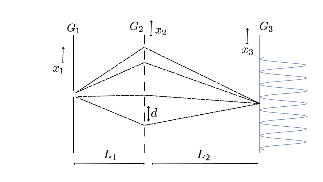
Figure 2: The Talbot effect [26]. The intensity modulation of the molecules immediately after the passage of the diffraction grating $G_{2}$, Fig. 3, is reproduced, due to the sum over paths, at an imaging plane $G_{3}$ placed at definite distances $L_{2}$, related to the Talbot length $L_{T}=\frac{d^{2}}{\lambda_{dB}}\;$ from $G_{2}$.

Figure 3: The intensity pattern of the atom (or molecule) behind the diffraction grating $G_{2}$. Each peak corresponds to a slit opening.

The rough estimate of the quantum ratio for the atom or molecule in these experiments is discussed in [1]: the result is shown in Table 2.

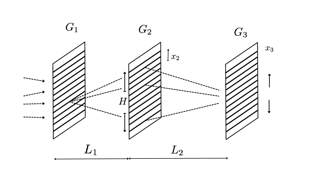
Figure 4: Talbot-Lau interferometer. $G_{2}$ is the diffraction grating. Thick lines are the slit openings. $G_{3}$ is a transmission-scanning grating movable vertically. $G_{1}$ are the source slits.

Particle	mass	$L_{0}$	$R_{q}$	$Q$	Exp	Miscl
$Ag$	$108$	$1.44$	$0.2$	$\sim 10^{6}$	[15]	Stern-Gerlach
$Na$	$23$	$2.27$	$0.5/0.75$	$\sim 10^{6}$	[22]
$C_{70}$	$840$	$9.4$	$16$	$\sim 10^{7}$	[20, 19, 21]	$T\ll 2000K$
$C_{70}$	$840$	$9.4$	$\sim 0.001$	$\sim 10^{3}$	[21]	$T\geq 3000K$

Table 2: The size ($L_{0}$), the quantum fluctuation range ($R_{q}$) and the quantum ratio $Q\equiv R_{q}/L_{0}$ of atoms and molecules in various experiments. The mass is in atomic unit ($au$); $L_{0}$ is given in Angström ($\AA$); $R_{q}$ is in $mm$. In all cases, the momentum of the atom (molecule), their masses, the size of the whole experimental apparatus, thus the time interval involved, are such that the quantum diffusion of their (transverse) wave packets are negligible.

2.4.1 Remark on “matter wave”

A familiar expression used often in the articles on the atomic and molecular interferometry [17]-[25] is “matter wave”. It might appear to summarize nicely the characteristic feature of quantum-mechanics: “wave-particle duality”. Actually, such an expression is more likely to obscure the essential quantum mechanical features of these processes, rather than illuminating them. It appears to imply that the beams of atoms or molecules somehow behave as a sort of wave: this is not an accurate description of the processes studied. The wave-particle duality of de Broglie, the core concept of quantum mechanics, is the property of each single quantum-mechanical particle, and not of any unspecified collective motion of particles in the beam . This point was demonstrated experimentally by Tonomura et. al.[27] in a double-slit electron interferometry experiment à la Young, with exemplary clarity.

Exactly the same phenomena occur in any atomic or molecular interferometry. As the correlation among the atoms or molecules in the beam is negligible (as it should be), and the position of each final atom/molecule is apparently random, the resulting interference fringes such as manifested in the Talbot (or the Talbot-Lau) interferometers, is all the more surprising and interesting. What these experiments show goes much deeper into the heart of QM, than the words, “matter wave” or “wave-particle duality”, might suggest.

2.5 A reflection

Thus the electron, being an elementary particle, is quantum mechanical ($L_{0}=0,$ $Q=\infty$). On the other hand, it is well known that an electron decoheres in $10^{-13}$ sec, in the $300K$ atmosphere at $1$ atm pressure [28]-[34]. So what is happening? The only sensible conclusion to draw is that decoherence and classical limit are two distinct concepts: they should not be identified. Decoherence does not mean in itself that the particle affected becomes classical, even though the classical behavior of macroscopic bodies do require decoherence (see Appendix B).

3 Decoherence does not imply classical

This observation, which follows at once from the concept of Quantum Ratio applied to the elementary particles, can have far-reaching consequences. Let us discuss this question with a few atomic or molecular processes.

3.1 Stern-Gerlach processes with small and large spins

First we discuss the SG process again, in more detail, in three different regimes, (i) a pure QM process; (ii) the environmental decoherence (an incoherent, mixed state); and (iii) for a classical particle. The main aim is to highlight the differences between these different physics situations as sharply as possible.

3.1.1 Pure spin $\frac{1}{2}$ state

In the Stern-Gerlach experiment for a spin $\frac{1}{2}$ particle, the wave function

$$\Psi=\psi_{1}({\bf r},t)|\!\uparrow\rangle+\,\psi_{2}({\bf r},t)|\!\downarrow\rangle\;.$$ (3.1)

splits, in an inhomogeneous magnetic field, into two subpackets, each obeying the Schrödinger equation,

$$i\hbar\frac{\partial}{\partial t}\psi_{1,2}=\left(\frac{{\bf p}^{2}}{2m}\pm\mu_{B}B_{z}\right)\psi_{1,2}\;.$$ (3.2)

For certain subtleties in the Stern-Gerlach processes, see Appendix C and [35, 36].

From (3.2) and their complex conjugates, the Ehrenfest theorems for spin-up and spin-down components follow separately,

$$\frac{d}{dt}\langle{\bf r}\rangle_{1}=\langle{\bf p}/{m}\rangle_{1}\;,\quad\frac{d}{dt}\langle{\bf p}\rangle_{1}=-\langle\nabla(\mu_{B}B(z))\rangle_{1}\;;$$ (3.3)

$$\frac{d}{dt}\langle{\bf r}\rangle_{2}=\langle{\bf p}/{m}\rangle_{2}\;,\quad\frac{d}{dt}\langle{\bf p}\rangle_{2}=+\langle\nabla(\mu_{B}B(z))\rangle_{2}\;,$$ (3.4)

where $\langle{\bf r}\rangle_{1}\equiv\langle\psi_{1}|{\bf r}|\psi_{1}\rangle$, etc. Nevertheless, the two subwavepackets $\psi_{1}$ and $\psi_{2}$ remain in coherent superposition.

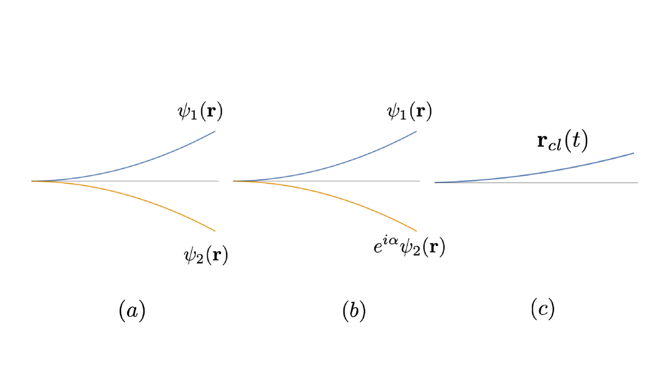
Figure 5: The spin-up and spin-down sub wavepackets of the silver atom evolve independently under the Schrödinger equation, both in the vacuum (fig.(a), pure state) and in a weak environment (3.6)-(3.8) (fig.(b)), where the decoherence is represented by an unknown, to-be-averaged-over, relative phase $\alpha$ between $\psi_{1}({\mathbf{r}})$ and $\psi_{2}({\mathbf{r}})$. Fig.(c) represents a unique classical trajectory.

3.1.2 Spin $\frac{1}{2}$ and weak decoherence

When the system is immersed in an environment, it rapidly decoheres. The density matrix in the position representation gets reduced at times $t\gg 1/\Lambda$, to a diagonal form

$$\psi({\bf r})\psi({\bf r}^{\prime})^{*}\to\psi_{1}({\bf r})\psi_{1}({\bf r}^{\prime})^{*}|\!\uparrow\rangle\langle\uparrow|+\psi_{2}({\bf r})\psi_{2}({\bf r}^{\prime})^{*}|\!\downarrow\rangle\langle\downarrow|\;,\qquad|{\bf r}_{1}-{\bf r}_{2}|\gg\lambda\;,$$ (3.5)

where $\Lambda$ is the decoherence rate [28]-[34] and $\lambda$ is the de Broglie wavelength of the environment particles. The diagonal density matrix (3.5) means that each atom is now either near ${\bf r}_{1}$ or near ${\bf r}_{2}$. The prediction for the SG experiment is however similar to the case of spin-mixed state: it cannot be distinguished from the prediction $|c_{1}|^{2}:|c_{2}|^{2}$ for the relative intensities of the two image bands in the case of the pure state.

Actually, the study of the effects of the environment particles is a complex, and highly nontrivial problem, as it involves many factors such as the density and flux of these particles, the pressure, the average temperature, kinds of the particles present and the type of interactions, and so on [28]-[34]. A simple statement such as (3.5) might sound as an oversimplification.

Without going into details, we may nevertheless enlist the basic conditions under which the result (3.5) can be considered reliable. Following [30], we introduce the decoherence time $\tau_{dec}\sim 1/\Lambda_{dec}$, as a typical timescale over which the decoherence takes place. Also the dissipation time $\tau_{diss}$ may be considered, as a timescale in which the loss of the energy, momentum of the atom under study due to the interactions with the environmental particles, become significant . We need to consider also a typical quantum diffusion time, $\tau_{diff}$, and finally, the transition time, $\tau_{trans}$, the interval of time the atom spends between the source slit to the image screen. Summarizing, we consider the time scales

$$\tau_{dec}\ll\tau_{trans}\ll\tau_{diff},\tau_{diss}\;.$$ (3.6)

The first inequality tells that the motion of the wave packets is much slower than the typical decoherence time. Consider the atom at some point, where it is described by a split wave packet of the form (3.1), with their centers separated by

$$|{\bf r}_{1}-{\bf r}_{2}|\gg a\;,$$ (3.7)

where $a$ is the size of the original wavepacket. We may then treat such an atom as if it were at rest, and take into account the rapid decoherence processes studied in [28]-[34] first (a sort of Born-Oppenheimer approximation). Furthermore, let us also take the typical de Broglie wavelength $\lambda$ of the environment particles such that

$$a\ll\lambda\ll|{\bf r}_{1}-{\bf r}_{2}|\;.$$ (3.8)

Namely, the environment particles can resolve between the split wave packets, but not the interior of each of the subpackets, $\psi_{1}({\bf r})$ or $\psi_{2}({\bf r}).$

Under the conditions (3.6)-(3.8), each of the split wave packets proceeds just as in the pure case (no environment) reviewed in Sec. 3.1.1, whose average position and momentum (i.e., the expectation values) obey Newton’s equations, (3.3), (3.4). Each of the subpackets describes a quantum particle, in a (position) mixed state, that is, either near ${\bf r}_{1}$ or ${\bf r}_{2}$. After leaving the region of the SG magnets, it is just a (pure-state) wave packet $\psi_{1}({\bf r})$ or $\psi_{2}({\bf r})$. The two wave functions however no longer interfere, Fig. 5 (b), in contrast to the pure split wave packet studied in Sec. 3.1.1, Fig. 5 (a).

Note that if any of the conditions (3.6)-(3.8) are violated the motion of the atom would be very different. For instance, $\tau_{diss}\ll\tau_{trans}$ would mean a totally random motion for the atom. Even in such a case, though, the effects of the environment-induced decoherence/disturbance are quite distinct from that of a classical motion of a particle, with a unique, well-defined trajectory, discussed below, Fig. 5 (c).

3.1.3 Classical particle

A classical particle, with the magnetic moment directed towards

$${\bf n}=(\sin\theta\cos\phi,\sin\theta\sin\phi,\cos\theta)\;,$$ (3.9)

is described by Newton’s equation,

$$m\,{\dot{\bf r}}={\bf p}\;,\qquad\frac{dp_{x}}{dt}=\frac{dp_{y}}{dt}=0\;,\quad\frac{dp_{z}}{dt}=F_{z}=-\frac{\partial}{\partial z}{\boldsymbol{\mu}\cdot{\bf B}}\;.$$ (3.10)

It traces a unique, well defined trajectory (Fig. 5 c). The way the unique trajectory for a classical particle emerges from quantum mechanics has been discussed in [5], where the magnetic moment is an expectation value

$$\sum_{i}\langle\Psi|({\hat{\boldsymbol{\mu}}}_{i}+\frac{e_{i}{\hat{\boldsymbol{\ell}}}_{i}}{2m_{i}c})|\Psi\rangle={\boldsymbol{\mu}}\;,$$ (3.11)

taken in the internal bound-state wave function $\Psi$ and $\mu_{i}$ and $\frac{e_{i}{\bf\ell}_{i}}{2m_{i}c}$ denote the intrinsic magnetic moment and one due to the orbital motion of the $i$-th constituent atom (molecule); $i=1,2,\ldots,N$. Clearly, in general, the considerations made in Sec. 3.1.1 and Sec. 3.1.2 for a spin $1/2$ atom, with a doubly split wave packet, cannot be generalized simply to (or compared with) a classical body (3.11) with $N\sim O(10^{23})$.

3.2 An infinite spin puzzle

Generally many spins inside a macroscopic body are oriented in random, different directions. But above all, the particles inside are bound in atomic, molecular and in crystaline structures. A bound particle does not split à la Stern-Gerlach under an inhomogeneous magnetic field, because the bound-state Hamiltonian does not allow that .

But what about a body made of many component spin $\frac{1}{2}$, all oriented in the same direction (e.g., a magnetized piece of metal)? Does such a body, with large spin, split in many sub wave packets in a strongly inhomogeneous magnetic field? The question is whether the three conditions recognized in [5] for the emergence of classical mechanics for a macroscopic body with a unique trajectory, reviewed in Appendix B here, are indeed sufficient. Or, is some extra condition, or a new unknown mechanism, needed, to suppress possible wide spreading of the wave function into many sub-packets under an inhomogeneous magnetic field?

The answer turns out to be simple, but somewhat unexpected [1, 6]. Consider the state of spin $j$, oriented towards a definite spatial direction, ${\mathbf{n}}$, that is ,

$${\hat{\mathbf{J}}}^{2}\,|j,{\mathbf{n}}\rangle=j(j+1)|j,{\mathbf{n}}\rangle\,,\qquad({\hat{\mathbf{J}}}\cdot{\mathbf{n}})\,|j,{\mathbf{n}}\rangle=j\,|j,{\mathbf{n}}\rangle\,,$$ (3.12)

where ${\mathbf{n}}$ is a unit vector directed towards $(\theta,\phi)$ direction,

$${\mathbf{n}}=(\sin\theta\cos\phi,\sin\theta\sin\phi,\cos\theta)\;.$$ (3.13)

The projection of this state on various eigenstates of $J_{z}$ is give by

$$|j,{\mathbf{n}}\rangle=\sum_{k=0}^{2j}c_{k}\,|j,m\rangle\;,\qquad m=-j+k\;,$$ (3.14)

$$c_{k}={\binom{2j}{k}}^{1/2}\,e^{i(j-k)\phi}\left(\cos\tfrac{\theta}{2}\right)^{k}\left(\sin\tfrac{\theta}{2}\right)^{2j-k}\;,\qquad\sum_{k=0}^{2j}|c_{k}|^{2}=1\;,$$ (3.15)

Under a magnetic field with a strong gradient towards the ${\hat{z}}$ direction, the wave function of a small spin particle will split in sub wavepackets, with relative weight proportional to $|c_{k}|^{2}$, ($j_{z}=-j+k$), as in Fig. 5 (a) for spin $\frac{1}{2}$, or as in Fig. 6 for a spin $\frac{13}{2}$ particle.

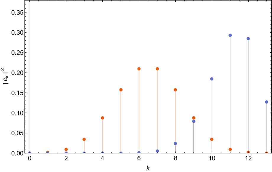
Figure 6: The distribution $|c_{k}|^{2}$ in $k$, i.e. in possible values of $J_{z}=m$, $-j\leq m\leq j$ ($m=-j+k$) for a spin $j=13/2$ particle in the state (3.14), (3.15), with $\theta=\pi/2$ (center, orange dots) or with $\theta=\pi/4$ (right, blue dots).

But the behavior for $j\to\infty$ turns out to be quite different. See Fig. 7, for a spin $j=20000.$ Such a behavior can be understood by using Stirling’s formula in (3.15). One finds, for $n$ and $k=j+m$ both large with $x=k/n$ fixed, the following distribution in different values of $m=-j+k$,

$$|c_{k}|^{2}\simeq e^{nf(x)}\;,\qquad x=k/n=(j+m)/2j\;,$$ (3.16)

where

$$f(x)=-x\log x-(1-x)\log(1-x)+2x\log\cos\tfrac{\theta}{2}+2(1-x)\log\sin\tfrac{\theta}{2}\;.$$ (3.17)

The saddle-point approximation valid at $n\to\infty$, yields

$$f(x)\simeq-\frac{(x-x_{0})^{2}}{x_{0}(1-x_{0})}\;,\qquad x_{0}=\cos^{2}\tfrac{\theta}{2}\;,$$ (3.18)

and therefore

$$\sum_{k}|c_{k}|^{2}(\cdots)\longrightarrow\int_{0}^{1}dx\,\delta(x-x_{0})\,(\cdots)$$ (3.19)

in the $n\to\infty$ ($x=k/n$ fixed) limit. The narrow peak position $x=x_{0}$ corresponds to (see Eq.(3.14))

$$J_{z}=m=n(x-\tfrac{1}{2})=j\,(2\cos^{2}\tfrac{\theta}{2}-1)=j\,\cos\theta\;.$$ (3.20)

This means that a large spin ($j\gg\hbar$) quantum particle with spin directed towards ${\mathbf{n}}$, in a Stern-Gerlach setting with an inhomogeneous magnetic field, moves along a single trajectory of a classical particle with $J_{z}=j\,\cos\theta$, instead of spreading over a wide range of split sub-packet trajectories covering $-j\leq m\leq j$.

This (perhaps) somewhat surprising result appears to indicate that quantum mechanics (QM) takes care of itself, so to speak, in ensuring that a large spin particle ($j/\hbar\to\infty$) behaves classically, at least for these particular states $|j,{\mathbf{n}}\rangle$. No extra conditions are necessary. See [6], however, for more careful discussion on the quantum mechanical nature of generic large spin states, far from spin coherent states $|j,{\mathbf{n}}\rangle$.

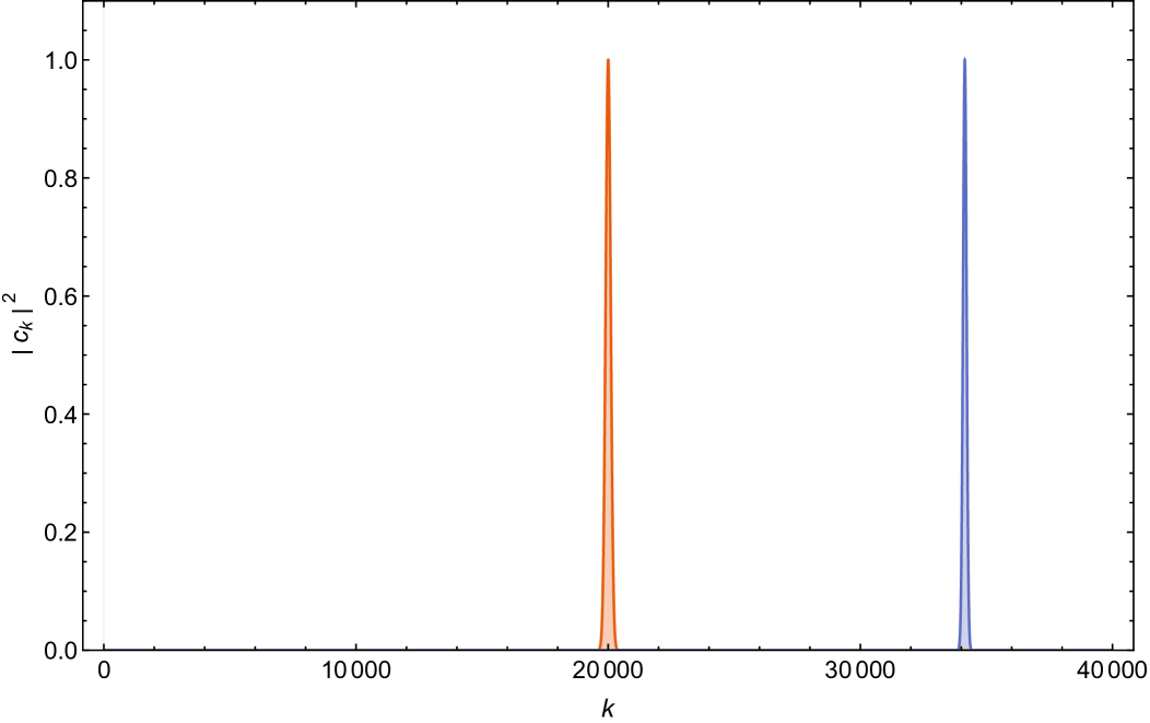
Figure 7: The distribution $|c_{k}|^{2}$ ($J_{z}=m=-j+k$) as in Fig. 6 but for a spin $j=2\cdot 10^{5}$, for $\theta=\pi/2$ (center, orange peak) or $\theta=\pi/4$ (right, blue peak). This figure is drawn by using the approximation (3.16) and (3.17), rather than the exact formula, (3.14), (3.15).

3.3 Tunnelling molecules

Another example of a process in which the distinction between decoherence and the classical limit can be neatly illustrated is a molecular (or atomic) beam, spilt in transverse direction $(x,y)$,

$$\Psi=e^{ip_{0}z/\hbar}\psi(x,y)\;,\qquad\psi(x,y)=c_{1}\psi_{1}(x,y)+c_{2}\psi_{2}(x,y)\;,$$ (3.21)

where $\psi_{1}$ and $\psi_{2}$ are narrow (free) wave packets centered at ${\bf r}_{1}=(x_{1},y_{1})$ and ${\bf r}_{2}=(x_{2},y_{2})$, respectively. Actually, we take a wave packet, $\chi_{p_{0}}(p,z)$, also for the longitudinal wave function by considering a linear superposition of the plane waves $e^{ipz/\hbar}$ with momentum $p$ narrowly distributed around $p=p_{0}$. For instance, a Gaussian distribution in $p$, $\sim e^{-(p-p_{0})^{2}/b^{2}}$, will yield a Gaussian longitudinal wave packet in $z$ of width $\sim 2\hbar/b$. At times much less than the characteristic diffusion time $t\ll\frac{2m\hbar}{b^{2}}$, the particle is approximately described by the wave function ,

$$\Psi_{asymp}\sim e^{ip_{0}z/\hbar}e^{-ip_{0}^{2}t/2m\hbar}e^{-\tfrac{b^{2}}{4\hbar^{2}}(z-\tfrac{p_{0}t}{m})^{2}}\;\psi(x,y)\;.$$ (3.22)

Assume that such a particle is incident from $z=-\infty$ ($t=-\infty$), moves towards right (increasing $z$), and hits a potential barrier (Fig. 8),

$$V=\begin{cases}0\;,&|z|>a,\\ V(z)\;,&-a<z<a\end{cases}$$ (3.23)

whose height is above the energy of the particle, approximately given by the longitudinal kinetic energy, $E\simeq\tfrac{p_{0}^{2}}{2m}$. As the longitudinal and transverse motions are factorized, the relative frequencies of finding the particle on both sides of the barrier (barrier penetration and reflection) at large $t$ can be calculated by the standard one-dimensional QM. The answer is well known: for instance the tunnelling frequency is given, in the semi-classical approximation, by

$$P_{tunnel}=|c|^{2}\,,\qquad c\sim e^{-\int_{-a_{0}}^{a_{0}}dz\,\sqrt{2m(V(z)-E)}/\hbar}\;,$$ (3.24)

($V(z)-E>0,\,\,-a_{0}<z<a_{0}$). The particle on the right of the barrier is described by the wave function

$$\Psi_{penetrated}\simeq c\,\Psi_{asymp}=c\,e^{ip_{0}z/\hbar}e^{-ip_{0}^{2}t/2m\hbar}e^{-\tfrac{b^{2}}{4\hbar^{2}}(z-\tfrac{p_{0}t}{m})^{2}}\;\psi(x,y)\;,$$ (3.25)

where $c$ is the transmission coefficient (3.24). The transverse, coherent superposition of the two sub wavepackets, (3.21), remains intact. See Fig. 8.

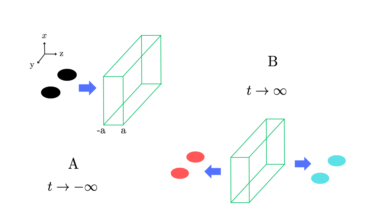
Figure 8: On the left figure (A), an atom (molecule) arrives from $z=-\infty$ and moves towards the potential barrier $V(z)$ at $-a<z<a$ (independent of $x$ and $y$). It is described by a wave packet (split in the transverse direction as in (3.21)). The wave function of the particle at $t\to\infty$, shown in the right part (B), contains both the reflected and transmitted waves. The coherent superposition of the two sub wavepackets in the $(xy)$ plane remains intact.

Now reconsider the whole process, with the region left of the barrier ($z<-a$) immersed in air. The precise decoherence rate depends on several parameters, but the incident particles get decohered in a very short time in general, as in (3.5) [28]-​[34]. The particle at the left of the barrier is now a mixture: each atom (molecule) is either near ${\bf r}_{1}=(x_{1},y_{1})$ or ${\bf r}_{2}=(x_{2},y_{2})$ in the transverse plane, just as in (3.5). But when it hits the potential barrier it will tunnel through it, with the relative frequencies (3.24), and will emerge on the other side of the barrier as a free particle. It has the wave function, (3.25), with $\psi(x,y)$ replaced by $\psi_{1}(x,y)$, with relative frequency $|c_{1}|^{2}/(|c_{1}|^{2}+|c_{2}|^{2})$, or by $\psi_{2}(x,y)$, with frequency $|c_{2}|^{2}/(|c_{1}|^{2}+|c_{2}|^{2}$). It is a statistical mixture, but each is a pure quantum mechanical particle. See Fig. 9.

Our discussion here assumes that the air molecules are just energetic enough (their de Broglie wave length small enough) to resolve the transverse split wave packets (see (3.5)), but are much less energetic than the longitudinal kinetic energy $\tfrac{p_{0}^{2}}{2m}$ and that their flux is sufficiently small. In writing (3.25) we assumed that the effects of the environment particles on the longitudinal wave packet are small, even though the tunnel frequency may be somewhat modified, as it is very sensitive to its energy.

Obviously, in a much warmer and denser environment the effects of the scatterings on our molecule would be more severe, and the tunnelling rate would become considerably smaller. Even then, our atom (or molecule) remains quantum mechanical .

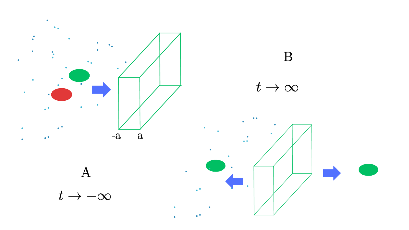
Figure 9: On the left figure (A), an atom (molecule) arrives from $z=-\infty$ and moves towards the potential barrier at $-a<z<a$, as in Fig. 8. But, this time, the half space on the left of the potential barrier contains air. The molecule is now in a mixed state due to the environment-induced decoherence. Its (transverse) position density matrix became diagonal: it is either near $(x_{1},y_{1})$ or near $(x_{2},y_{2})$. The wave function of the particle at $t\to\infty$, shown in the right part (B), contains still a small transmitted wave as well as the reflected wave, however without coherent superposition of two transverse wave packets.

3.4 Cosmic rays

The cosmic rays (neutrinos, gamma, proton, etc.) coming out of the hot and dense environments of star’s interiors, once out, propagate freely in the intergalaxy space (a good approximation of the vacuum) as pure-state quantum mechanical particles.

4 Conclusion

The notion that the elementary particles are quantum mechanical, is usually taken for granted in high-energy physics (and in general, physics) communities. However, as we are asking here whether a molecule, a macromolecule, or larger particles, are quantum mechanical or classical, and under which conditions, it perhaps makes sense to ask whether or not the elementary particles are quantum mechanical, and if so, why. Introduction of the concept of the Quantum Ratio, and the related criterion, allow us to answer at once this question affirmatively, and to explain why.

We are however not claiming that this is a new, original idea about the quantum mechanical nature of the elementary particles. Perhaps one should go back to early $70^{\prime}$ s when the standard model [8, 9, 10, 11] of the quarks and leptons has been established as the correct theory of the fundamental interactions. The laws underlying the Nature seem to be written in terms of a unifying language of local, quantum field theory of nonAbelian gauge interactions [42]. And these are relativistic, quantum theories of particles.

The fact that elementary particles, thus electron and photon, and to certain extent the atoms and small molecules, are always quantum mechanical, means that even if the CM of a macroscopic body behaves classically, the internal microscopic degrees of freedoms continue to be quantum mechanical. This is so, even if in a warm environment such as interiors of biological systems these particles will suffer from various sorts of decoherence effects. Decoherence however does not mean that the system affected becomes classical: the latter becomes a mixture. It is possible that certain quantum mechanical phenomena such as the tunnel effect survive decoherence, as discussed in Sec. 3.3. These questions constitute one of the important research themes in the nascent science of quantum biology [7].

A bi-product of these considerations concerns the abstract concept of “a particle of mass $m$”, familiar both in quantum-mechanics and classical-mechanics textbooks, to formulate model systems such as a harmonic oscillator. The Quantum Ratio [1], and general ideas how Newton’s equations emerge from quantum mechanics for macroscopic bodies [5], tell us however that a model based on such an abstract concept of “particle”, without any information about its size $L_{0}$ and its composition, cannot be used to explain the emergence of classical mechanics.

In a recent attempt to clean up our understanding of the so-called quantum measurement problems [2], a particular emphasis was given to the particle nature of the fundamental entities of our world. This is indeed the reason for the spacetime local (i.e., event-like) nature of any quantum measurement process at its core. And this, combined with the unique classical state of matter (the reading) of the macroscopic measuring device after each measurement, explains what is often perceived as the “wave function collapse”.

The Quantum Ratio [1] and the notion that the elementary particles are quantum mechanical, might have been thought as the final outcome of the series of considerations on the Great Twin Puzzles of Physics Today. It is heartwarming though to realize that, actually, the idea of pointlike quantum nature of the fundamental entities of our world was also at the very starting point [2] and characterizes the whole chain of reasonings which followed [3, 4, 5, 6], and which has eventually led to the idea of the Quantum Ratio [5, 1].

Appendix A Elementary particles

The elementary particles known today (as of the year 2024) are the quarks, leptons (electron, muon, $\tau$ lepton), the three types of neutrinos, and the gauge bosons (the gluons, $W$, $Z$ bosons and the photon), plus the Higgs boson (with mass $125,35$ GeV/$c^{2}$), with masses [14],

$2.16$ ($u$)	$4.67$ ($d$)	$93.4$ ($s$)	$1.27\cdot 10^{3}$ ($c$)	$4.18\cdot 10^{3}$ ($b$)	$172.7\cdot 10^{3}$ ($t$)

Table 3: The quark masses in MeV/$c^{2}$; the errors not indicated. $1$ MeV$/c^{2}\simeq 1.782661\cdot 10^{-27}$ g

$0.51099895$ ($e$)	$105.658$ ($\mu$)	$1776.86$ ($\tau$)	$m_{\nu}\neq 0$ ; $m_{\nu}<0.8$ eV$/c^{2}$

Table 4: The lepton masses. The $e$, $\mu$ and $\tau$ masses are given in MeV$/c^{2}$.

photon	gluons	${W^{\pm}}$ (GeV$/c^{2}$)	${Z}$ (GeV$/c^{2}$)
$0$	$0$	$80.377\pm 0.012$	$91.1876\pm 0.0021$

Table 5: Gauge bosons and their masses

Appendix B Newton’s equation for a macroscopic body

The conditions needed for the CM of an isolated macroscopic body at finite body temperatures to obey Newton’s equations have been investigated in great care in [5]. They are

• For macroscopic motions (for which $\hbar\simeq 0$) the Heisenberg relation does not limit the simultaneous determination – the initial condition – of the position and momentum;

• The absence of quantum diffusion, due to a large mass (a large number of atoms and molecules composing the body);

• A finite body temperature, implying the thermal decoherence and mixed-state nature of the body.

Under these conditions, the CM of an isolated macroscopic body has a unique trajectory. Newton’s equations for it follow from the Ehrenfest theorem. See Ref. [5] for discussions on various subtleties and for the explicit derivation of Newton’s equation under external gravitational forces, under weak, static, smoothly varying external electromagnetic fields, and under a harmonic-oscillator potential. Somewhat unexpectedly, the environment-induced decoherence [28]-[34] which is extremely effective in rendering macroscopic states in a finite-temperature environment a mixture, is found not to be the most essential element for the derivation of classical mechanics from quantum mechanics.

Appendix C A subtle face of the Stern-Gerlach experiment

The Hamiltonian is given by

$$H=\frac{{\bf p}^{2}}{2m}+V\;,\qquad V=-{\boldsymbol{\mu}\cdot{\bf B}}\;,$$ (C.1)

$${\boldsymbol{\mu}}=\mu_{B}\,g\,{\mathbf{s}}\;,\qquad\partial B_{z}/\partial z\neq 0\;,$$ (C.2)

where $\mu_{B}=\frac{e\hbar}{2m_{e}c}$ is the Bohr magneton. We recall the well-known fact that the gyromagnetic ratio $g\simeq 2$ of the electron and the spin magnitude $1/2$ approximately cancel, so $\mu_{B}$ is the magnetic moment, in the case of the atoms such as $A_{g}$, where a single outmost electron provides the total spin $\tfrac{1}{2}$.

An example of the inhomogeneous field ${\bf B}$ appropriate for the Stern-Gerlach experiment is [36, 35]

$${\bf B}=(0,B_{y},B_{z}),\qquad B_{y}=-b_{0}\,y,\quad B_{z}=B_{0}+b_{0}\,z\;$$ (C.3)

which satisfy $\nabla\cdot{\bf B}=\nabla\times{\bf B}=0$. The constant field $B_{0}$ in the $z$ direction must be large,

$$|B_{0}|\gg|b_{0}\,y|\;.$$ (C.4)

in the relevant region of $(y,z)$ of the experiment. The wave function of the spin $\frac{1}{2}$ particle entering the SG magnet has the form,

$$\Psi={\tilde{\psi}}_{1}({\bf r},t)|\!\uparrow\rangle+\,{\tilde{\psi}}_{2}({\bf r},t)|\!\downarrow\rangle\;.$$ (C.5)

obeying the Schrödinger equation,

$$i\hbar\frac{d}{dt}\Psi=H\,\Psi\;.$$ (C.6)

By redefining the wave functions for the upper and down spin components as

$${\tilde{\psi}}_{1}({\bf r},t)=e^{i\mu_{B}B_{0}t/\hbar}\psi_{1}({\bf r},t)\;,\qquad{\tilde{\psi}}_{2}({\bf r},t)=e^{-i\mu_{B}B_{0}t/\hbar}\psi_{2}({\bf r},t)\;,$$ (C.7)

one finds that the up- and down- spin components $\psi_{1}$ and $\psi_{2}$ satisfy the separate Schrödinger equations [36]

$$i\hbar\frac{\partial}{\partial t}\psi_{1}=\left(\frac{{\bf p}^{2}}{2m}-\mu_{B}b_{0}z\right)\psi_{1}\;,\qquad i\hbar\frac{\partial}{\partial t}\psi_{2}=\left(\frac{{\bf p}^{2}}{2m}+\mu_{B}b_{0}z\right)\psi_{2}\;.$$ (C.8)

This is because the term $\propto-\mu_{y}B_{y}=-(g\mu_{B}b)s_{y}$ in the Hamiltonian (C.1) mixing the two components $\psi_{1,2}$ has acquired a rapidly oscillating phase factor,

$$\pm i\mu_{B}\,b_{0}y\,e^{\mp 2i\mu_{B}B_{0}t/\hbar}\;,$$ (C.9)

hence can be safely neglected. The condition (C.4) is crucial here.

As explained in [35], this can be classically understood as the spin precession effect around the large constant magnetic field $B_{0}\hat{z}$, thanks to which the forces on the particle in the transverse ($\hat{x},\hat{y}$) directions average out to zero . The only significant force it receives is due to the inhomogeneity in $B_{z}$, (C.2), which deflects the atom in the $\pm\hat{z}$ direction.

References

- [1] Konishi K and Elze H T 2024 “The Quantum Ratio”, Symmetry 2024, 16(4), 427; [arXiv:2402.10702 [quant-ph]].
- [2] Konishi K 2022 “Quantum fluctuations, particles and entanglement: a discussion towards the solution of the quantum measurement problems,” Int. Journ. Mod. Phys. A 37 2250113 [arXiv:2111.14723 [quant-ph]].
- [3] Konishi K 2023 “Quantum fluctuations, particles and entanglement: solving the quantum measurement problems,” J. Phys. Conf. Ser. 2533, no.1, 012009 [arXiv:2302.08892 [quant-ph]].
- [4] Konishi K 2024 “On the Negative Result Experiments in Quantum Mechanics,” Entropy 26, no.11, 958 (2024) [arXiv:2310.01955 [quant-ph]].
- [5] Konishi K 2023 “Newton’s equations from quantum mechanics for a macroscopic body in the vacuum”, Int. Journ. Mod. Phys. A 38 2350080 [arXiv:2209.07318 [quant-ph]].
- [6] Konishi K and Menta R 2024 “Large Angular Momentum”, [arXiv:2404.14931 [quant-ph]].
- [7] Al-Khalili J, Mc-Fadden J, Kim Y, et.al. 2021 “Quantum Biology: An Update and Perspective”, Quantum Reports 3, 80, number: 1 Publisher: Multidisciplinary Digital Publishing Institute.
- [8] Weinberg S 1967 “A model of Leptons”, Phys. Rev. Lett. 19 1264.
- [9] Salam A 1968 “Weak and electromagnetic interactions,” in Elementary Particle Theory, ed. N. Svartholm, Almqvist Forlag AB, 367.
- [10] Glashow S L, Iliopoulos J and Maiani L 1970, “Weak Interactions with Lepton-Hadron Symmetry,” Phys. Rev. D 2, 1285.
- [11] Fritzsch H, Gell-Mann M and Leutwyler H 1973 ”Advantages of the color octet gluon picture”, Physics Letters 47 B, 365.
- [12] Wilson K G 1983 “The Renormalization Group and Critical Phenomena”, Rev. Mod. Phys. 55, 583.
- [13] Coleman S 1971 “Dilatations”, in “Aspect of Symmetry - selected Erice Lectures” Cambridge University Press (1985).
- [14] Workman R L et.al., (Particle Data Group) 2022 Prog. Theor. Exp. Phys. 2022 083C01 and 2023 update.
- [15] Gerlach W and Stern O 1922 “Der experimentelle Nachweis der Richtungsquantelung im Magnetfeld”, Zeitschrift für Physik. 9 (1) 349.
- [16] Keith D W, Ekstrom C R, Turchette Q A, and Prichard D E 1991 “An interferometer for Atoms”, Phys. Rev. Lett. 66 2693.
- [17] Brand C, Troyer S, Knobloch C, Cheshinovsky O and Arndt M A 2021 “Single, double and triple-slit diffraction of molecular matter waves”, Am. J. of Phys. 89, 1132 arXiv:2108.06565v2 [quant-ph]
- [18] Arndt M, Nairz O, Vos-Andreae J, Keller C, van der Zouw G, Zeilinger A 1999 “Wave-particle duality of molecules”, Nature 401 680.
- [19] Brezger B, Arndt M and Zeilinger A, “Concepts for near-field interferometers with large molecules”, J. Opt. B: Quantum Semiclass. Opt. 5 (2003) S82–S89.
- [20] Brezger B, Hackermüller L, Uttenthaler S, Petschinka J, Arndt M, and Zeilinger A 2002 “Matter-Wave Interferometer for Large Molecules” Phys. Rev. Lett. 88.100404
- [21] Hackermüller L, Hornberger K, Brezger B, Zeilinger A, Arndt M 2004 “Decoherence of matter waves by thermal emission of radiation”, Nature, 427, 711. arXiv:quant-ph/0402146.
- [22] Chapman M S, Ekstrom C R, Hammond T D, Schmiedmayer J, Tannian B E, Wehinger S, and Pritchard D E 1995 “Near-field imaging of atom diffraction gratings: The atomic Talbot effect”, Phys. Rev. A, 51, R14-R17.
- [23] Nowak S, Kurtsiefer Ch, Pfau T, and David C 1997 ”High-order Talbot fringes for atomic matter waves,” Opt. Lett. 22, 1430.
- [24] Clauser J F and Li S 1994 “Talbot-vonLau atom interferometry with cold slow potassium”, Phys. Rev. A 49, R2213.
- [25] Bateman J, Nimmrichter S, Hornberger K, Ulbricht H 2014 “Near-field interferometry of a free-falling nanoparticle from a point-like source”, Nature communications, 5, Article number: 4788.
- [26] Talbot H F Esq. F.R.S. (1836) LXXVI. “Facts relating to optical science. No. IV”, The London, Edinburgh, and Dublin Philosophical Magazine and Journal of Science, 9:56, 401-407
- [27] Tonomura A, Endo J, Matsuda T, Kawasaki T and Ezawa H 1989 “Dimonstration of single-electron buildup of interference pattern”, American Journal of Physics 57, 117.
- [28] Joos E and Zeh H D 1985 “The emergence of classical properties through interaction with the environment”, Z. Phys. B 59, 223-243 (1985).
- [29] Zurek W H (1991) “Decoherence and the Transition from Quantum to Classical”, Physics Today 44, 10, 36 (1991).
- [30] Tegmark M 1993 “Apparent wave function collapse caused by scattering,” Found. Phys. Lett. 6, 571 (1993) [arXiv:gr-qc/9310032 [gr-qc]].
- [31] Hansen K and Campbell E E B 1988 “Thermal radiation from small particles”, Phys. Rev. E 58, 5477.
- [32] Tegmark M 2000 “Importance of quantum decoherence in brain processes”, Phys. Rev. E 61 4194.
- [33] Joos E, Zeh H D, Kiefer C, Giulini D, Kupsch J, Stamatescu I O 2002 “Decoherence and the Appearance of a Classical World in Quantum Theory”, Springer.
- [34] Zurek W H 2003 “Decoherence, einselection, and the quantum origins of the classical,” Rev. Mod. Phys. 75, 715-775 [arXiv:quant-ph/0105127 [quant-ph]].
- [35] Alstrøm P, Hjorth P and Mattuck R 1982 “Paradox in the classical treatment of the Stern-Gerlach experiment”, Am. J. Phys. 50, 697.
- [36] Platt D E 1992 “A modern analysis of the Stern-Gerlach experiment”, Am. J. Phys. 60, 306.
- [37] Radcliffe J M 1971 “Some properties of coherent spin states”, J. Phys. A: Gen. Phys. 4 (1971).
- [38] Arecchi F T, Courtens E, Gilmore R and Thomas H 1972 “Atomic Coherence States in Quantum Optics”, Phys. Rev. A 6, 2211 (1972).
- [39] Lieb E H 1973 “The Classical Limit of Quantum Spin Systems”, Commun. Math. Phys. 31, 327.
- [40] Puri R R 1997 “Coherent and squeezed states on physical basis”, Pramana - J Phys 48 787.
- [41] Aravind P K 1999 “Spin coherent states as anticipators of the geometric phase”, Am. J. Phys. 67, 899.
- [42] ’t Hooft G 1980 “Why Do We Need Local Gauge Invariance in Theories With Vector Particles? An Introduction,” NATO Sci. Ser. B 59, 101-115 (1980).