LSD of the Commutator of two data Matrices

Abstract.

We study the spectral properties of a class of random matrices of the form $S_{n}^{-}=n^{-1}(X_{1}X_{2}^{*}-X_{2}X_{1}^{*})$ where $X_{k}=\Sigma_{k}^{1/2}Z_{k}$, $Z_{k}$’s are independent $p\times n$ complex-valued random matrices, and $\Sigma_{k}$ are $p\times p$ positive semi-definite matrices that commute and are independent of the $Z_{k}$’s for $k=1,2$. We assume that $Z_{k}$’s have independent entries with zero mean and unit variance. The skew-symmetric/skew-Hermitian matrix $S_{n}^{-}$ will be referred to as a random commutator matrix associated with the samples $X_{1}$ and $X_{2}$. We show that, when the dimension $p$ and sample size $n$ increase simultaneously, so that $p/n\to c\in(0,\infty)$, there exists a limiting spectral distribution (LSD) for $S_{n}^{-}$, supported on the imaginary axis, under the assumptions that the joint spectral distribution of $\Sigma_{1},\Sigma_{2}$ converges weakly and the entries of $Z_{k}$’s have moments of sufficiently high order. This nonrandom LSD can be described through its Stieltjes transform, which satisfies a system of Marčenko-Pastur-type functional equations. Moreover, we show that the companion matrix $S_{n}^{+}=n^{-1}(X_{1}X_{2}^{*}+X_{2}X_{1}^{*})$, under identical assumptions, has an LSD supported on the real line, which can be similarly characterized.

1. Introduction

Since the seminal works on the behavior of the empirical distribution of eigenvalues of large-dimensional symmetric matrices and sample covariance matrices by Wigner [24] and Marčenko and Pastur [15] respectively, there have been extensive studies on establishing limiting behavior of various classes of random matrices. With the traditional definitions of sample size and dimension for multivariate observations, one may refer to the high-dimensional asymptotic regime where these quantities are proportional as the random matrix regime. In the random matrix regime, there have been discoveries of nonrandom limits for the empirical distribution of sample eigenvalues of various classes of symmetric or hermitian matrices. Notable classes of examples include matrices known as Fisher matrices (or “ratios” of independent sample covariance matrices ([27], [28]), signal-plus-noise matrices ([9]) arising in signal processing, sample covariance corresponding to data with separable population covariance structure ([26],[6]), with a given variance profile ([13], symmetrized sample autocovariance matrices associated with stationary linear processes ([12], [14], [3]), sample cross covariance matrix ([4]), etc. Studies of the spectra of these classes of random matrices mentioned above are often motivated by various statistical inference problems.

Commutators play an important role in quantum mechanics, for example in describing Heisenberg’s uncertainty principle. Using combinatorial techniques, [16] derived the spectral distribution of the commutator of two free random variables. [8] established the Tetilla Law, namely, the law of the commutator of two free semicircular random variables, which is absolutely continuous with a density having a closed form expression. [18] investigated the statistical properties of multiplicative commutators, i.e. matrices of the type $C=uvu^{-1}v^{-1}$, when $u$ and $v$ are independent random matrices, uniformly distributed with respect to the Haar measure of the groups $U(N)$ and $O(N)$. [19] analyzed the distribution of the anti-commutator of two free Poisson random variables. [23] proved the existence of limiting spectral distributions for the commutator and the anti-commutator of two Hermitian random matrices, rotated independently with respect to one another, as the dimension grows to infinity.

Partially motivated by these, we look at a different class of ”commutator/ anti-commutator matrices”, namely that of two independent rectangular data matrices under certain regularity conditions. In this paper, we study the asymptotic behavior of the spectra of random commutator matrices under the random matrix regime and discuss a potential application to a inference problem involving covariance matrices.

As the setup for introducing these random matrices, suppose we have $p$-variate independent samples of the same size $n$ (expressed as $p\times n$ matrices) denoted by $X_{k}=[X_{k,1}:\cdots:X_{k,n}]$, for $k=1,2$, from two populations with zero mean and variances $\Sigma_{1}$ and $\Sigma_{2}$ respectively. We shall study the spectral properties of the matrix $S_{n}^{-}$ defined as

$$S_{n}^{-}:=n^{-1}[X_{1},X_{2}]:=n^{-1}(X_{1}X_{2}^{*}-X_{2}X_{1}^{*})$$

where $X_{k}^{*}$ denotes the Hermitian conjugate of $X_{k}$. Given the analogy with a commutator matrix, we shall refer to $S_{n}^{-}$ as a “sample commutator matrix” associated with the data $(X_{1},X_{2})$. A distinctive feature of $S_{n}^{-}$ is that it is skew-symmetric, so that the eigenvalues of $S_{n}^{-}$ are purely imaginary numbers. Analogously, we also study the properties of the Hermitian companion matrix $S_{n}^{+}$ which we shall refer to as the anti-commutator matrix.

$$S_{n}^{+}:=n^{-1}\{X_{1},X_{2}\}:=n^{-1}(X_{1}X_{2}^{*}+X_{2}X_{1}^{*})$$

As a primary contribution, in this paper we establish the existence of limits for the empirical spectral distribution (ESD) of $S_{n}^{-}$, when $p,n\to\infty$ such that $p/n\to c\in(0,\infty)$, and describe the limiting spectral distribution (LSD) through its Stieltjes transform, under additional technical assumptions on the statistical model. This LSD can be described as a unique solution of a pair of functional equations describing its Stieltjes transform. We also derived results related to continuity of the solution as a function of the limiting population spectrum of $\Sigma_{1},\Sigma_{2}$. The proof techniques are largely based on the matrix decomposition based approach popularized by [2]. Furthermore, in the special case when $\Sigma_{1}=I_{p}=\Sigma_{2}$, we completely describe the LSD of $S_{n}^{-}$ as a mixture distribution on the imaginary axis with a point mass at zero (only if $c>2$), and a symmetric distribution with a density. Establishment of this result requires a very careful analysis of the Stieltjes transform of the LSD of $S_{n}^{-}$, since the latter satisfies a cubic equation for each complex argument. The density function of the continuous component of the LSD can be derived in a closed (albeit complicated) functional form that depends only on the value of $c$.

As a further contribution, we are able to derive the asymptotic behavior of the spectrum of the companion matrix $S_{n}^{+}$. The results follow a similar pattern, which is why we state these results in parallel with our main results (about the spectral distribution of $S_{n}^{-}$).

As a potential application, consider a set of $n$ paired $p$-dimensional observations from a multivariate Gaussian distribution. Denote the two samples as $X_{1}=\Sigma^{\frac{1}{2}}Z$ and $X_{2}=\Sigma^{\frac{1}{2}}W$ where $W=(W_{ij}),Z=(Z_{ij})\in\mathbb{R}^{p\times n}$ having independent entries with zero mean and unit variance. The experimenter suspects an element-wise dependence, i.e., $\operatorname{Corr}(Z_{ij},W_{ij})=\rho$, and would like to test the hypothesis $H_{0}:\rho=0$ against $H_{1}:\rho\neq 0$.

We can characterize this dependence in terms of another independent Gaussian random matrix $V=(V_{ij})$, with i.i.d. standard normal entries, as follows. Observe that, distributionally, we have the following representation:

$$W_{ij}=\rho Z_{ij}+\sqrt{1-\rho^{2}}V_{ij},\qquad\mbox{for}~i=1,\ldots,p,~j=1,\ldots,n.$$

We see that

(1.1) $$n^{-1}[X_{1},X_{2}]=\Sigma^{\frac{1}{2}}[Z,W]\Sigma^{\frac{1}{2}} =n^{-1}\Sigma^{\frac{1}{2}}(ZW^{*}-WZ^{*})\Sigma^{\frac{1}{2}}$$

$$=n^{-1}\Sigma^{\frac{1}{2}}\bigg{(}Z(\rho Z^{*}+\sqrt{1-\rho^{2}})V^{*})-(\rho Z+\sqrt{1-\rho^{2}}V)Z^{*}\bigg{)}\Sigma^{\frac{1}{2}}$$

$$=n^{-1}\sqrt{1-\rho^{2}}\Sigma^{\frac{1}{2}}(ZV^{*}-VZ^{*})\Sigma^{\frac{1}{2}}=n^{-1}\sqrt{1-\rho^{2}}\Sigma^{\frac{1}{2}}[Z,V]\Sigma^{\frac{1}{2}}$$

Note that under the null hypothesis, $Z$ and $W$ are independent, thus allowing us to derive the limiting spectral distribution of $n^{-1}[X_{1},X_{2}]$ using the results derived in this paper. Even under the alternative, (1.1) allows us to derive the limiting spectral distribution of $n^{-1}[X_{1},X_{2}]$, by making used of the fact that $Z$ and $V$ are independent. Indeed, under the alternative, the only change in the form of the LSD is that the support shrinks by a factor of $\sqrt{1-\rho^{2}}$. This result can be helpful in deriving asymptotic properties of test statistics for testing $H_{0}:\rho=0$ vs. $H_{1}:\rho\neq 0$ if such statistics are derived from linear functionals of the eigenvalues of $[X_{1},X_{2}]$.

A related question was studied by [4], who studied the spectral behavior of the sample cross-covariance matrix $C_{n}:=n^{-1}X_{1}X_{2}^{T}$, under the assumption that entries of $(X_{1,ij},X_{2,ij})$ are independent, with a common correlation $\rho$, and with mean 0 and variance 1. This corresponds to the setting above with $\Sigma=I_{p}$. Under these assumptions, when $p/n\to c\in(0,\infty)$, they showed that $C_{n}$ converges in an algebraic sense, and the limiting spectral moments depend on only $\rho$ and $c$. Observe that $S_{n}^{-}=n^{-1}[X_{1},X_{2}]$ may be seen as an skew-Hermitized version of $C_{n}$. Analogously, the anti-commutator can be viewed as the Hermitian version of the cross-covariance matrix.

The rest of the paper is organized as follows. Section 2 describes the preliminaries and the model setup. Section 3 introduces new definitions to handle distributions over the imaginary axis. This is important since we will be working with skew-Hermitian matrices. As such, existing results related to metrics and convergence of measures over the real line are tweaked to handle measures over the imaginary axis. The main result of this paper is Theorem 4.3 in Section 4 that covers the most general case with arbitrary pairs of commuting variance matrices. In Section 5, we present the special case when $\Sigma_{1}=\Sigma_{2}$. The next section deals with the special case when $\Sigma_{1}=I_{p}=\Sigma_{2}$. Finally, results regarding the anti-commutator matrix are derived in Section 7.

2. Model and preliminaries

Notations: $\mathbbm{i}$ denotes $\sqrt{-1}$. $\mathbb{R}$ and $\mathbbm{i}\mathbb{R}$ denote the real and the imaginary axes of the complex plane respectively. $\mathbb{C}^{+}$ and $\mathbb{C}^{-}$ denote the upper and the lower halves of the complex plane respectively excluding the real axis, i.e. $\mathbb{C}^{\pm}=\{u+\mathbbm{i}v:u\in\mathbb{R},\pm v>0\}$. Similarly, $\mathbb{C}_{L}:=\{-u+\mathbbm{i}v:u>0,v\in\mathbb{R}\}$ and $\mathbb{C}_{R}:=\{u+\mathbbm{i}v:u>0,v\in\mathbb{R}\}$ denote the left and right halves of the complex plane respectively excluding the imaginary axis. $\Re(z)$ and $\Im(z)$ denote the real and imaginary parts respectively of $z$. The norm of a vector $x$ will be denoted as $||x||$ and the operator norm of a matrix $A$ is denoted by $||A||_{op}$.

Definition 2.1.

For a skew-Hermitian matrix $S\in\mathbb{C}^{p\times p}$ with eigenvalues $\{\mathbbm{i}\lambda_{j}\}_{j=1}^{p}$, we define the empirical spectral distribution (ESD) $F$ of $S$ as

(2.1) $$F^{S}:\mathbbm{i}\mathbb{R}\rightarrow[0,1];\hskip 8.53581ptF^{S}(\mathbbm{i}x)=\frac{1}{p}\sum_{j=1}^{p}\mathbbm{1}_{\{\lambda_{j}\leq x\}}$$

Remark 2.2.

Note that $-\mathbbm{i}S$ is Hermitian with real eigenvalues $\{\lambda_{j}\}_{j=1}^{p}$. Reconciling (2.1) with the standard definition of ESD for Hermitian matrices (e.g. Section 2 of [21]), we thus have

(2.2) $$F^{S}(\mathbbm{i}x)=F^{-\mathbbm{i}S}(x)\hskip 5.69054pt\forall x\in\mathbb{R}$$

In (2.2), we have used the same notation, i.e. $F^{A}$ to denote the ESD of Hermitian and skew-Hermitian matrices alike. It is to be understood that the argument of the function will be real or imaginary depending on the matrix being Hermitian or skew-Hermitian respectively.

Definition 2.3.

Let $\{\lambda_{1j},\lambda_{2j}\}_{j=1}^{p}$ represent the eigenvalues of two commuting positive semi-definite matrices $\Sigma_{1},\Sigma_{2}\in\mathbb{C}^{p\times p}$ respectively. We define the joint empirical spectral distribution (JESD) of the two matrices as follows.

(2.3) $$H(s,t):=F^{\Sigma_{1},\Sigma_{2}}(s,t):=\frac{1}{p}\sum_{j=1}^{p}\mathbbm{1}_{\{0\leq\lambda_{1j}\leq s,0\leq\lambda_{2j}\leq t\}};\quad s,t\in\mathbb{R}$$

Suppose $\{Z_{1}^{(n)},Z_{2}^{(n)}\}_{n=1}^{\infty}$ are sequences of random matrices each having dimension $p\times n$ such that $p/n\rightarrow c\in(0,\infty)$. The entries have zero mean, unit variance and uniformly bounded moments of order $4+\eta_{0}$ for some $\eta_{0}>0$. Let $\Sigma_{1n},\Sigma_{2n}\in\mathbb{C}^{p\times p}$ be a sequence of random commuting positive semi-definite matrices such that the JESD of $\{\Sigma_{1n},\Sigma_{2n}\}_{n=1}^{\infty}$ converge weakly to a probability distribution function $H$ (supported on a subset of $\mathbb{R}_{+}^{2}$) in an almost sure sense. We are interested in the limiting behavior (as $p,n\rightarrow\infty$) of the ESDs of matrices of the type

(2.4) $$S_{n}^{\pm}:=\frac{1}{n}X_{1}^{(n)}(X_{2}^{(n)})^{*}\pm\frac{1}{n}X_{1}^{(n)}(X_{2}^{(n)})^{*}\text{, where }$$

$$X_{k}^{(n)}:=(\Sigma_{kn})^{\frac{1}{2}}Z_{k}^{(n)}\text{ for }k\in\{1,2\}$$

Henceforth, for simplicity we will use $Z_{k}$ (corresp., $X_{k}$) to denote $Z_{k}^{(n)}$ (corresp., $X_{k}^{(n)}$), respectively for $k=1,2$.

We define the following central objects associated with our work.

Definition 2.4.

$S_{n}:=\frac{1}{n}(X_{1}X_{2}^{*}-X_{2}X_{1}^{*})=\frac{1}{n}\sum_{r=1}^{n}(X_{1r}X_{2r}^{*}-X_{2r}X_{1r}^{*})$

Definition 2.5.

$S_{nj}:=\frac{1}{n}\sum_{r\neq j}(X_{1r}X_{2r}^{*}-X_{2r}X_{1r}^{*})$ for $1\leq j\leq n$

Additionally for $z\in\mathbb{C}_{L}$, we define the following.

Definition 2.6.

$Q(z):=(S_{n}-zI_{p})^{-1}$ is the resolvent of $S_{n}$

Definition 2.7.

$Q_{-j}(z):=(S_{nj}-zI_{p})^{-1}$ is the resolvent of $S_{nj}$ where $1\leq j\leq n$

Remark 2.8.

For $z\in\mathbb{C}_{L}$, it is easy to see that any eigenvalue $\lambda$ of $S_{n}-zI_{p}$ satisfies $|\lambda|\geq|\Re(z)|$. Thus we have $||Q(z)||_{op}\leq 1/|\Re(z)|$. Similarly, we also have $||Q_{-j}(z)||_{op}\leq 1/|\Re(z)|$.

Definition 2.9.

We denote the JESD of $(\Sigma_{1n},\Sigma_{2n})$ as $H_{n}$ for $n\in\mathbb{N}$.

3. Stieltjes Transforms of Measures on the imaginary axis

The existing definition of Stieltjes transform and basic results deal with the weak convergence of probability measures supported on (subsets of) the real line. Since we will be dealing with skew-Hermitian matrices which have purely imaginary (or zero) eigenvalues, we modify/ develop existing definitions/ results related to convergence of measures. We will start by defining a distribution function over the imaginary axis.

Let $X$ be a purely imaginary random variable. We give the most natural definition for the distribution function $F$ of $X$. Let $\overline{F}$ be the distribution function of $-\mathbbm{i}X$, the real counterpart of $X$. Then, $F$ is defined as follows.

(3.1) $$F(\mathbbm{i}x):=\overline{F}(x)\text{ for }x\in\mathbb{R}$$

It is clear that $F$ is the clockwise rotated version of $\overline{F}$. The analogous Levy metric between distribution functions $F,G$ on the imaginary axis can be defined as

(3.2) $$L_{im}(F,G):=L(\overline{F},\overline{G})$$

where $L(\overline{F},\overline{G})$ is the “standard” Levy distance between distributions $\overline{F},\overline{G}$ over the real line. Similarly, we define the uniform distance between $F$ and $G$ as

(3.3) $$||F-G||_{im}:=||\overline{F}-\overline{G}||$$

where $||\overline{F}-\overline{G}||$ represents the “standard” uniform metric between distributions over the real line. Therefore, using Lemma B.18 of [2] leads to the following analogous inequality between Levy and uniform metrics.

(3.4) $$L_{im}(F,G)=L(\overline{F},\overline{G})=\leq||\overline{F}-\overline{G}||=||F-G||_{im}$$

This will be important specifically in establishing the weak convergence of measures over the imaginary axis.

Definition 3.1.

(Stieltjes Transform) For a measure (not necessarily probability) $\mu$ supported on the imaginary axis, we define the Stieltjes Transform as follows.

(3.5) $$s_{\mu}:\mathbb{C}\backslash\operatorname{supp}(\mu)\rightarrow\mathbb{C},\hskip 8.53581pt\displaystyle s_{\mu}(z)=\int_{\mathbb{R}}\dfrac{\mu(dt)}{\mathbbm{i}t-z}$$

With this definition, we immediately observe the following properties. The proofs are exactly similar to those of the corresponding properties for Stieltjes Transforms of probability measures on the real line (for instance Section 2.1.2 of [7]).

1:

$s_{\mu}(.)$ is analytic on its domain and

(3.6) $$s_{\mu}(\mathbb{C}_{L})\subset\mathbb{C}_{R}\text{ and }s_{\mu}(\mathbb{C}_{R})\subset\mathbb{C}_{L}$$

2:

Let the total mass of $\mu$ be denoted by $M_{\mu}\geq 0$. Then a bound for the value of the transform at the point $z$ is given by

(3.7) $$|s_{\mu}(z)|\leq M_{\mu}/|\Re(z)|$$

3:

If a probability measure $\mu$ has a density at $\mathbbm{i}x$ where $x\in\mathbb{R}$, then

(3.8) $$f_{\mu}(x)=\dfrac{1}{\pi}\underset{\epsilon\downarrow 0}{\lim}\hskip 2.84526pt\,\Re(s_{\mu}(-\epsilon+\mathbbm{i}x))$$

4:

If a probability measure $\mu$ has a point mass at $\mathbbm{i}x$ where $x\in\mathbb{R}$, then

(3.9) $$\mu(\{x\})=\underset{\epsilon\downarrow 0}{\lim}\hskip 2.84526pt\,\epsilon s_{\mu}(-\epsilon+\mathbbm{i}x)$$

5:

For $\mathbbm{i}a,\mathbbm{i}b$ continuity points of a probability measure $\mu$, we have

(3.10) $$\mu([\mathbbm{i}a,\mathbbm{i}b])=\dfrac{1}{\pi}\underset{\epsilon\downarrow 0}{\lim}\hskip 2.84526pt\int_{a}^{b}\Re(s_{\mu}(-\epsilon+\mathbbm{i}x)dx$$

Recall the definition of $S_{n}$ from (2.4). Let $S_{n}=P\Lambda P^{*}$ be a spectral decomposition of $S_{n}$ with $\{\mathbbm{i}\lambda_{j}\}_{j=1}^{p}$ being the $p$ purely imaginary (or zero) eigenvalues of $S_{n}$. In light of Definition (3.5), we have the following expression for the Stieltjes Transform of $F^{S_{n}}$, the ESD of $S_{n}$.

Definition 3.2.

$s_{n}(z):=\dfrac{1}{p}\operatorname{trace}(Q(z))=\dfrac{1}{p}\sum_{j=1}^{p}\dfrac{1}{\mathbbm{i}\lambda_{j}-z}$

Let $P^{*}\Sigma_{kn}P:=A^{(k)}=(a_{ij}^{(k)})$ for $k=1,2$. With this notation, we define another quantity that will play a key role in our work.

Definition 3.3.

$\textbf{h}_{n}(z):=(h_{1n}(z),h_{2n}(z))^{T}$ where $h_{kn}(z):=\dfrac{1}{p}\operatorname{trace}(\Sigma_{kn}Q(z))=\dfrac{1}{p}\sum_{j=1}^{p}\dfrac{a_{jj}^{(k)}}{\mathbbm{i}\lambda_{j}-z}$

It is easy to see that $h_{kn}(\cdot)$ is the Stieltjes Transform of the discrete measure (say $\mu_{kn}$) that allocates a mass of $a_{jj}^{(k)}/p$ at the point $\mathbbm{i}\lambda_{j}$ for $1\leq j\leq p$ and $k=1,2$. At this point, we make a note of the total variation norm of the underlying measure ($\mu_{kn}$) which will be used later.

(3.11) $$TV(\mu_{kn})=\frac{1}{p}\sum_{j=1}^{p}a_{jj}^{(k)}=\frac{1}{p}\operatorname{trace}(A^{(k)})=\frac{1}{p}\operatorname{trace}(\Sigma_{kn})$$

Lemma 3.4.

For a probability distribution $F$ over the imaginary axis, let $s_{F}$ be the Stieltjes Transform (in the sense of Definition 3.5). For any random variable $X\sim F$, let $\overline{F}$ represent the distribution of the real-valued random variable $-\mathbbm{i}X$. Then, the Stieltjes Transform (in the standard sense) of $\overline{F}$ at $z\in\mathbb{C}^{+}$ is given by

(3.12) $$s_{\overline{F}}(z)=\mathbbm{i}s_{F}(\mathbbm{i}z)$$

Proof.

For $x\in\mathbb{R}$, it is clear that $dF(\mathbbm{i}x)=d\overline{F}(x)$. Note that $z\in\mathbb{C}^{+}$ implies that $\mathbbm{i}z\in\mathbb{C}_{L}$. Thus, we have

(3.13) $$s_{\overline{F}}(z)=\int\frac{d\overline{F}(x)}{x-z}=\int\frac{dF(\mathbbm{i}x)}{-\mathbbm{i}(\mathbbm{i}x-\mathbbm{i}z)}=\mathbbm{i}\int\frac{dF(y)}{y-\mathbbm{i}z}=\mathbbm{i}s_{F}(\mathbbm{i}z)$$

∎

The following is an analogue of a result linking convergence of Stieltjes transforms to the weak convergence of measures on the real axis.

Proposition 3.5.

For $n\in\mathbb{N}$, let $s_{n}(\cdot)$ be the Stieltjes transform of $F_{n}$, a probability distribution over the imaginary axis. If $s_{n}(z)\xrightarrow{}s(z)$ for $z\in\mathbb{C}_{L}$ and $\underset{y\rightarrow+\infty}{\lim}ys(-y)=1$, then $F_{n}\xrightarrow{d}F$ where $s(\cdot)$ is the Stieltjes transform of $F$, a probability distribution over the imaginary axis.

Proof.

The proof can be adapted with similar arguments from Theorem 1 of [11] which is stated below.

“Suppose that ($P_{n}$) are real Borel probability measures with Stieltjes transforms ($S_{n}$) respectively. If $\underset{n\rightarrow\infty}{\lim}S_{n}(z)=S(z)$ for all z with $\Im(z)>0$, then there exists a Borel probability measure $P$ with Stieltjes transform $S_{P}=S$ if and only if

$$\underset{y\rightarrow\infty}{\lim}\mathbbm{i}yS(\mathbbm{i}y)=-1$$

in which case $P_{n}\rightarrow P$ in distribution.” ∎

Proposition 3.6.

Let $m_{G}(.)$ be the Stieltjes Transform of a probability measure $G$ on the imaginary axis. Then $G$ is differentiable at $\mathbbm{i}x_{0}$, if $m^{*}(\mathbbm{i}x_{0})\equiv\underset{z\in\mathbb{C}_{L}\rightarrow\mathbbm{i}x_{0}}{\lim}\Re(m_{G}(z))$ exists and its derivative at $\mathbbm{i}x_{0}$ is $({1}/{\pi})m^{*}(\mathbbm{i}x_{0})$.

Proof.

The proof is similar to that of Theorem 2.1 of [5] which is stated below.

“Let G be a p.d.f. and $x_{0}\in\mathbb{R}$. Suppose $\Im(m_{G}(x_{0}))\equiv\underset{z\in\mathbb{C}^{+}\rightarrow x_{0}}{\lim}\Im(m_{G}(z))$ exists. Then G is differentiable at $x_{0}$, and its derivative is $({1}/{\pi})\Im(m_{G}(x_{0}))$.” ∎

We mention the Vitali-Porter Theorem (Section 2.4, [20]) below without proof.

Theorem 3.7.

Let $\{f_{n}\}_{n=1}^{\infty}$ be a locally uniformly bounded sequence of analytic functions in a domain $\Omega$ such that $\underset{n\rightarrow\infty}{\lim}f_{n}(z)$ exists for each $z$ belonging to a set $E\subset\Omega$ which has an accumulation point in $\Omega$. Then $\{f_{n}\}_{n=1}^{\infty}$ converges uniformly on compact subsets of $\Omega$ to an analytic function.

We state the Grommer-Hamburger Theorem (page 104-105 of [25]) below without proof.

Theorem 3.8.

Let $\{\mu_{n}\}_{n=1}^{\infty}$ be a sequence of measures in $\mathbb{R}$ for which the total variation is uniformly bounded.

1. If $\mu_{n}\xrightarrow{d}\mu$, then $S(\mu_{n};z)\rightarrow S(\mu;z)$ uniformly on compact subsets of $\mathbb{C}\backslash\mathbb{R}$.

2. If $S(\mu_{n};z)\rightarrow S(z)$ uniformly on compact subsets of $\mathbb{C}\backslash\mathbb{R}$, then S(z) is the Stieltjes transform of a measure on $\mathbb{R}$ and $\mu_{n}\xrightarrow{d}\mu$.

4. LSD under arbitrary commuting pair of scaling matrices

Before stating the main result of the paper, we first define a few functions.

Definition 4.1.

$\boldsymbol{\rho}:\mathbb{C}^{2}\backslash\{(z_{1},z_{2})\in\mathbb{C}^{2}:z_{1}z_{2}\neq-1\}\rightarrow\mathbb{C}^{2}$ such that $\boldsymbol{\rho}(z_{1},z_{2})=\bigg{(}\dfrac{z_{2}}{1+z_{1}z_{2}},\dfrac{z_{1}}{1+z_{1}z_{2}}\bigg{)}^{T}$

Letting $\boldsymbol{\rho}(z_{1},z_{2})=(\rho_{1}(z_{1},z_{2}),\rho_{2}(z_{1},z_{2}))^{T}$, we have the following relationships.

(4.1) $$\Re(\rho_{1}(z_{1},z_{2}))=\frac{\Re(z_{2}(1+\bar{z}_{1}\bar{z}_{2}))}{|1+z_{1}z_{2}|^{2}}=\frac{\Re(z_{2})+\Re(z_{1})|z_{2}|^{2}}{|1+z_{1}z_{2}|^{2}}$$

(4.2) $$\Re(\rho_{2}(z_{1},z_{2}))=\frac{\Re(z_{1}(1+\bar{z}_{1}\bar{z}_{2}))}{|1+z_{1}z_{2}|^{2}}=\frac{\Re(z_{1})+\Re(z_{2})|z_{1}|^{2}}{|1+z_{1}z_{2}|^{2}}$$

Remark 4.2.

It is clear that for $\textbf{z}=(z_{1},z_{2})\in\mathbb{C}_{R}^{2}$, we have $\boldsymbol{\rho}(\textbf{z}):=(\rho_{1}(\textbf{z}),\rho_{2}(\textbf{z}))^{T}\in\mathbb{C}_{R}^{2}$ or $\boldsymbol{\rho}(\mathbb{C}_{R}^{2})\subset\mathbb{C}_{R}^{2}$

Theorem 4.3.

Main Theorem: Suppose the following conditions hold.

$T_{1}$:

$c_{n}:=\dfrac{p}{n}\rightarrow c\in(0,\infty)$

$T_{2}$:

Entries of $Z_{1},Z_{2}$ are independent, zero mean, unit variance and have a uniform bound on moments of order $4+\eta_{0}$ for some $\eta_{0}>0$. $Z_{1}$ and $Z_{2}$ are independent.

$T_{3}$:

$\Sigma_{1n}\Sigma_{2n}=\Sigma_{2n}\Sigma_{1n}$ for all $n\in\mathbb{N}$

$T_{4}$:

$H_{n}\xrightarrow{d}H$ a.s. where $H$ is a non-random bi-variate probability distribution on $\mathbb{R}_{+}^{2}$ with support not contained entirely in the real or the imaginary axis.

$T_{5}$:

There exists a constant $D_{0}>0$ such that

(4.3) $$\underset{n\rightarrow\infty}{\limsup}\,\underset{k=1,2}{\max}\,\bigg{\{}\frac{1}{p}\operatorname{trace}(\Sigma_{kn}^{2})\bigg{\}}<D_{0}$$

Then, $F^{S_{n}}\xrightarrow{d}F$ where the Stieltjes Transform of $F$ at $z\in\mathbb{C}_{L}$ is characterized by the below set of equations.

(4.4) $$s_{F}(z) =\displaystyle\int_{\mathbb{R}_{+}^{2}}\frac{dH(\boldsymbol{\lambda})}{-z+\boldsymbol{\lambda}^{T}\boldsymbol{\rho}(c\textbf{h}(z))}$$

where $\textbf{h}(z)=(h_{1}(z),h_{2}(z))\in\mathbb{C}_{R}^{2}$ are unique numbers such that

(4.5) $$\textbf{h}(z) =\displaystyle\int_{\mathbb{R}_{+}^{2}}\frac{\boldsymbol{\lambda}dH(\boldsymbol{\lambda})}{-z+\boldsymbol{\lambda}^{T}\boldsymbol{\rho}(c\textbf{h}(z))}\text{, and }\boldsymbol{\lambda}=(\lambda_{1},\lambda_{2})^{T}$$

Moreover, $h_{1},h_{2}$ themselves are Stieltjes Transforms of measures (not necessarily probability measures) over the imaginary axis and continuous as functions of $H$. An equivalent characterization of the Stieltjes Transform is given by

(4.6) $$s_{F}(z) =\frac{1}{z}\bigg{(}\frac{2}{c}-1\bigg{)}-\frac{2}{cz}\bigg{(}\frac{1}{1+c^{2}h_{1}(z)h_{2}(z)}\bigg{)}\quad\text{for }z\in\mathbb{C}_{L}$$

NOTE: Throughout the paper we will be using bold symbols such as h, $\boldsymbol{\lambda}$, $\boldsymbol{\rho},\textbf{0}$ to denote vector quantities.

Remark 4.4.

The alternate characterization (4.6) of the Stieltjes Transform is useful when investigating presence of point mass at $0$ in the LSD. The detailed proofs of Theorem 4.3 presented later on will thus focus only on proving (4.4) and (4.5).

Remark 4.5.

For a fixed $z\in\mathbb{C}_{L}$, Theorem 4.24 states a result regarding the continuity of the solution to (4.5), i.e. $\textbf{h}(z)$ w.r.t. $H$ under a certain technical condition (4.19) and Assumption $T_{5}$. In the special case covered in Section 5, we prove a stronger result (Theorem 5.4) without requiring this technical condition or any assumption on spectral moment bounds.

Due to the conditions (i.e $T_{5}$) imposed on $\Sigma_{1n},\Sigma_{2n}$ in Theorem 4.3, there exists $0<C_{0}<\infty$ such that

(4.7) $$\underset{k=1,2}{\max}\,\bigg{\{}\underset{n\rightarrow\infty}{\limsup}\frac{1}{p}\operatorname{trace}(\Sigma_{kn})\bigg{\}}<C_{0}$$

and by Skorohod Representation Theorem and Fatou’s Lemma,

(4.8) $$\underset{k=1,2}{\max}\,\int\lambda_{k}dH(\boldsymbol{\lambda})\leq C_{0}$$

Remark 4.6.

The proof for existence of some solution of (4.5) can be done using a uniform bound only on the first spectral moments of $\Sigma_{1n},\Sigma_{2n}$ (i.e. 4.7). The proofs of uniqueness and continuity of the solution requires the second moments to be bounded, i.e. Assumption $T_{5}$.

Remark 4.7.

The assumptions on $\Sigma_{kn};k=1,2$ hold in an almost sure sense. Moreover, $H_{n}$ (defined in (2.3)) converges weakly to a non-random $H$ almost surely. By the end of this Section, we show that conditioning on $\Sigma_{kn};k=1,2$, $F^{S_{n}}$ converges weakly to a non-random limit $F$ that depends on $\Sigma_{kn}$ only through their non-random limit $H$. This result holds irrespective of whether $\Sigma_{kn}$ is random or not. Therefore, we will henceforth treat $\{\Sigma_{kn}\}_{n=1}^{\infty};k=1,2$ as a non-random sequence.

4.0.1. Proof of the equivalent characterization, i.e. (4.6) in Theorem 4.3

Proof.

The second expression for the Stieltjes Transform of the LSD $F$ in Theorem 4.3, i.e. (4.6) follows easily from (4.4) and (4.5). For $k=1,2$, we have

(4.9) $$h_{k}(z)=\int\frac{\lambda_{k}dH(\boldsymbol{\lambda})}{-z+\boldsymbol{\lambda}^{T}\boldsymbol{\rho}(c\textbf{h})}$$

$$\implies h_{k}(z)\rho_{k}(c\textbf{h}(z))=\int\frac{\lambda_{k}\rho_{k}(c\textbf{h}(z))dH(\boldsymbol{\lambda})}{-z+\boldsymbol{\lambda}^{T}\boldsymbol{\rho}(c\textbf{h}(z))}$$

$$\implies h_{1}(z)\rho_{1}(c\textbf{h}(z))+h_{2}(z)\rho_{2}(c\textbf{h}(z))=\int\frac{z-z+\lambda_{1}\rho_{1}(c\textbf{h}(z))+\lambda_{2}\rho_{2}(c\textbf{h}(z))}{-z+\lambda_{1}\rho_{1}(c\textbf{h}(z))+\lambda_{2}\rho_{2}(c\textbf{h}(z))}dH(\boldsymbol{\lambda})$$

$$\implies\frac{2ch_{1}(z)h_{2}(z)}{1+c^{2}h_{1}(z)h_{2}(z)}=zs_{F}(z)+1$$

$$\implies s_{F}(z)=-\frac{1}{z}+\frac{2}{cz}\frac{c^{2}h_{1}(z)h_{2}(z)}{1+c^{2}h_{1}(z)h_{2}(z)}$$

$$\implies s_{F}(z)=-\frac{1}{z}+\frac{2}{cz}\bigg{(}1-\frac{1}{1+c^{2}h_{1}(z)h_{2}(z)}\bigg{)}$$

$$\implies s_{F}(z)=\frac{1}{z}\bigg{(}\frac{2}{c}-1\bigg{)}-\frac{2}{cz}\bigg{(}\frac{1}{1+c^{2}h_{1}(z)h_{2}(z)}\bigg{)}$$

∎

Lemma 4.8.

Under the conditions of Theorem 4.3, if we instead had $H=\delta_{(0,0)}$, we have $F^{S_{n}}\xrightarrow{d}\delta_{(0,0)}$ a.s. For any probability distribution $H$ supported on $\mathbb{R}_{+}^{2}$, $\{F^{S_{n}}\}_{n=1}^{\infty}$ is a tight sequence.

The proof is given in Section B.2.1. Now we sketch the necessary steps to prove Theorem 4.3.

4.1. Sketch of the proof

Following [26], we will first prove the result under a set of extra assumptions. This will act as a stepping stone to prove the result under general conditions mentioned in Theorem 4.3. The assumptions are as follows.

4.1.1. Assumptions

• $A_{1}:$ There exists a constant $\tau>0$ such that $\underset{k=1,2}{\max}\bigg{(}\underset{n\in\mathbb{N}}{\operatorname{sup}}||\Sigma_{kn}||_{op}\bigg{)}\leq\tau$

• $A_{2}:$ For $k\in\{1,2\}$, $\mathbb{E}z_{ij}^{(k)}=0,|z_{ij}^{(k)}|\leq B_{n}$, where $B_{n}:=n^{a}$ with $\frac{1}{4+\eta_{0}}<a<\frac{1}{4}$ and $\eta_{0}>0$ is described in $T_{2}$ of Theorem 4.3

We provide below the sketch of the proof of Theorem 4.3 under Assumptions 4.1.1.

• First we show that for all $z\in\mathbb{C}_{L}$ equation (4.5) can have at most one solution within the class of analytic functions mapping $\mathbb{C}_{L}$ to $\mathbb{C}_{R}^{2}$. This is established in Theorem 4.11.

• For $k=1,2$, the sequences $\{h_{kn}(z)\}_{n=1}^{\infty}$ have at least one subsequential limit by Theorem 4.12. Every subsequential limit of $\{h_{kn}(z)\}_{n=1}^{\infty}$, $k=1,2$ satisfies (4.5) and moreover, they are Stieltjes Transforms of measures over the imaginary axis. This is done in Theorem 4.19. Thus (4.5) has a unique solution.

• Finally we will show that $s_{n}(z)\xrightarrow{a.s.}s_{F}(z)$ and $s_{F}$ satisfies the condition in Proposition 3.5. Therefore, $F^{S_{n}}\xrightarrow{d}F$ a.s. This is done in Theorem 4.19.

Next we show the above under the general conditions of Theorem 4.3. The idea is to construct sequences of matrices whose ESDs are close in uniform metric to that of $S_{n}$ but satisfy Assumptions 4.1.1. This allows us to use the above results. The outline of this part of the proof is provided in Theorem 4.20.

Definition 4.9.

For $0<b$, we define the bounded sector of $\mathbb{C}_{R}$ denoted by $\mathcal{S}(b)$ as follows.

(4.10) $$\mathcal{S}(b):=\{z\in\mathbb{C}_{R}:|\Im(z)|\leq\Re(z),|z|\leq b\}$$

Lemma 4.10.

(Location of Solution:) Let $z=-u+\mathbbm{i}v\in\mathbb{C}_{L}$ and $\textbf{h}=(h_{1},h_{2})\in\mathbb{C}_{R}^{2}$ be a solution to (4.5). Then for $k=1,2$,

1. Under the conditions of Theorem 4.3, we have $|h_{k}(z)|\leq C_{0}/u$ where $C_{0}$ is defined in (4.8).

2. If $|v|<u$ and $u$ is sufficiently large, then $|\Im(h_{k}(z))|\leq\Re(h_{k}(z)),k=1,2$.

The proof can be found in Section B.1.1.

Theorem 4.11.

(Uniqueness) For a bi-variate distribution $H$ supported on $\mathbb{R}_{+}^{2}$ and $c\in(0,\infty)$, there can be at most one solution to (4.5) within the class of analytic functions that map $\mathbb{C}_{L}$ to $\mathbb{C}_{R}^{2}$.

The proof can be found in Section B.1.2.

4.2. Existence of Solution under Assumptions 4.1.1

Theorem 4.12.

Compact Convergence: For $z\in\mathbb{C}_{L}$ and $k\in\{1,2\},$ $\mathcal{H}_{k}=\{h_{kn}:n\in\mathbb{N}\}$ are normal families.

Proof.

By Montel’s theorem (Theorem 3.3 of [22]), it is sufficient to show that $s_{n}$, $h_{1n}$ and $h_{2n}$ are uniformly bounded on every compact subset of $\mathbb{C}_{L}$. Let $K\subset\mathbb{C}_{L}$ be an arbitrary compact subset. Define $u_{0}:=\inf\{|\Re(z)|:z\in K\}$. Then it is clear that $u_{0}>0$. Then for arbitrary $z\in K$, using (3.7) we have

$$|s_{n}(z)|=\frac{1}{p}|\operatorname{trace}(Q(z))|\leq\frac{1}{|\Re(z)|}\leq\frac{1}{u_{0}}$$

Using $R_{5}$ of A.1, (4.7) and Remark 2.8, for sufficiently large $n$ and $k=1,2$, we have

(4.11) $$|h_{kn}(z)| =\frac{1}{p}|\operatorname{trace}(\Sigma_{kn}Q)|\leq\bigg{(}\frac{1}{p}\operatorname{trace}(\Sigma_{kn})\bigg{)}||Q(z)||_{op}\leq\frac{C_{0}}{|\Re(z)|}\leq\frac{C_{0}}{u_{0}}$$

∎

Remark 4.13.

Note that the proof relied simply on $T_{5}$ of Theorem 4.3 and not on Assumptions 4.1.1.

Theorem 4.14.

Deterministic Equivalent: Under Assumptions 4.1.1, for $z\in\mathbb{C}_{L}$, a deterministic equivalent for $Q(z)$ is given by

(4.12) $$\bar{Q}(z)=\bigg{(}-zI_{p}+\rho_{1}(c_{n}\mathbb{E}{\textbf{h}}_{n}(z))\Sigma_{1n}+\rho_{2}(c_{n}\mathbb{E}{\textbf{h}}_{n}(z))\Sigma_{2n}\bigg{)}^{-1}$$

Remark 4.15.

By (B.35), for large $n$, all the eigenvalues of $\bar{Q}(z)$ are non-zero for any $z\in\mathbb{C}_{L}$. This in particular implies that $\bar{Q}(z)$ is invertible for sufficiently large $n$ depending on $z$. The proof is given in Section C.

At this point, we define a few additional deterministic quantities that will serve as approximations to the random quantity $h_{kn}(z)$ for $z\in\mathbb{C}_{L}$ and $k=1,2$.

Definition 4.16.

$\tilde{\textbf{h}}_{n}(z):=(\tilde{h}_{1n}(z),\tilde{h}_{2n}(z))$ where $\tilde{h}_{kn}(z)=\frac{1}{p}\operatorname{trace}\{\Sigma_{kn}\bar{Q}(z)\}$, $k=1,2$, $z\in\mathbb{C}_{L}$

Under Assumptions 4.1.1, a direct consequence of Theorem 4.14 is as follows. For $k=1,2$, $z\in\mathbb{C}_{L}$, we have

(4.13) $$\left|\frac{1}{p}\operatorname{trace}(\Sigma_{kn}(Q(z)-\overline{Q}(z)))\right|\xrightarrow{a.s.}0\implies\left|h_{kn}(z)-\tilde{h}_{kn}(z)\right|\xrightarrow{a.s.}0$$

Definition 4.17.

$\bar{\bar{Q}}(z)=\bigg{(}-zI_{p}+\rho_{1}(c_{n}\tilde{\textbf{h}}_{n}(z))\Sigma_{1n}+\rho_{2}(c_{n}\tilde{\textbf{h}}_{n}(z))\Sigma_{2n}\bigg{)}^{-1}$

Definition 4.18.

$\tilde{\tilde{\textbf{h}}}_{n}(z):=(\tilde{\tilde{h}}_{1n}(z),\tilde{\tilde{h}}_{2n}(z))$ where $\tilde{\tilde{h}}_{kn}(z)=\frac{1}{p}\operatorname{trace}\{\Sigma_{kn}\bar{\bar{Q}}(z)\}$ , $k=1,2$

Using $T_{3}$ of Theorem 4.3, we can simplify $\tilde{h}_{kn}(z)$ and $\tilde{\tilde{h}}_{kn}(z)$ as follows.

(4.14) $$\tilde{\tilde{h}}_{kn}(z) =\int\frac{\lambda_{k}dH(\boldsymbol{\lambda})}{-z+\lambda_{1}\rho_{1}(c_{n}\mathbb{E}{\textbf{h}}_{n}(z))+\lambda_{2}\rho_{2}(c_{n}\mathbb{E}{\textbf{h}}_{n}(z))}$$

$$\tilde{\tilde{h}}_{kn}(z) =\int\frac{\lambda_{k}dH(\boldsymbol{\lambda})}{-z+\lambda_{1}\rho_{1}(c_{n}\tilde{\textbf{h}}_{n}(z))+\lambda_{2}\rho_{2}(c_{n}\tilde{\textbf{h}}_{n}(z))}$$

Note that by Theorem 4.14 and Lemma B.12, $\tilde{h}_{kn}(z),\tilde{\tilde{h}}_{kn}(z)$ are deterministic approximations to $h_{kn}(z)$. This serves as a critical step in the proof for the existence of the unique solution to (4.5).

Theorem 4.19.

Existence of solution: Under Assumptions 4.1.1, for $z\in\mathbb{C}_{L}$, we have

1:

For $k=1,2$, $h_{kn}(z)\xrightarrow{a.s.}h_{k}^{\infty}(z)$ where $h_{k}^{\infty}$ are Stieltjes transforms of measures over the imaginary axis

2:

$h_{1}^{\infty}(z),h_{2}^{\infty}(z)$ uniquely satisfy (4.5)

3:

For $z\in\mathbb{C}_{L}$, $s_{n}(z)\xrightarrow{a.s.}s_{F}(z)$ where $s_{F}(\cdot)$ is as defined in (4.4)

4:

$s_{F}(\cdot)$ satisfies $\underset{y\rightarrow+\infty}{\lim}ys_{F}(-y)=1$

The proof is given in Section D.

4.3. Existence of Solution under General Conditions

Theorem 4.19 proved the statement of Theorem 4.3 under Assumptions 4.1.1. We now repeat this but under the general conditions $T_{1}-T_{5}$ of 4.3. As a consequence of Theorem 4.19, for any fixed $\tau>0$, if we truncate $H$ at the point $(\tau,\tau)$, there exists a unique solution to (4.5) (with $H$ replaced by $H^{\tau}$) denoted by $\textbf{h}^{\tau}=(h_{1}^{\tau},h_{2}^{\tau})$ and the corresponding Stieltjes Transform of the LSD as $s^{\tau}$. Moreover, if the underlying distribution of $s^{\tau}$ is $F^{\tau}$, then, This serves as the basis for the proof.

Theorem 4.20.

Under the conditions of Theorem 4.3, for $z\in\mathbb{C}_{L}$, we have

1:

For $k=1,2$, $h_{k}^{\tau}(z)\xrightarrow{}h_{k}^{\infty}(z)$ where $h_{k}^{\infty}$ are Stieltjes transforms of measures over the imaginary axis

2:

$h_{1}^{\infty}(z),h_{2}^{\infty}(z)$ uniquely satisfy (4.5)

3:

For $z\in\mathbb{C}_{L}$, $s_{n}(z)\xrightarrow{a.s.}s_{F}(z)$ where $s_{F}(\cdot)$ is as defined in (4.4)

4:

$s_{F}(\cdot)$ satisfies $\underset{y\rightarrow+\infty}{\lim}ys_{F}(-y)=1$

Proof.

We construct a sequence of matrices similar to $\{S_{n}\}_{n=1}^{\infty}$ but satisfying A1-A2 of Assumptions 4.1.1. The steps below give an outline of the proof with the essential details shifted to individual modules wherever necessary.

Step1:

Let $H$ be a bi-variate distribution supported on $\mathbb{R}_{+}^{2}$. Consider the random vector $\textbf{e}=(e_{1},e_{2})\sim H$. For $\tau>0$, define $H^{\tau}$ as the distribution of $\textbf{e}^{\tau}:=(e_{1}^{\tau},e_{2}^{\tau})$ where $e_{k}^{\tau}:=e_{k}\mathbbm{1}_{\{e_{k}\leq\tau\}};k=1,2$

Step2:

For a p.s.d. matrix A and a fixed $\tau>0$, let $A^{\tau}$ represent the matrix obtained by replacing all eigenvalues of $A$ greater than $\tau$ with 0 in its spectral decomposition. Recall the definition of JESD from (2.3). It is clear that for any fixed $\tau>0$, as $n\rightarrow\infty$, we have

$$H_{n}^{\tau}:=F^{\Sigma_{1n}^{\tau},\Sigma_{2n}^{\tau}}\xrightarrow{d}H^{\tau}$$

However, we will choose $\tau>0$ such that $(\tau,\tau)$ is a continuity point of $H$. This will be essential in Section E.2.

Step3:

For $k=1,2$, let $\Lambda_{kn}:=\Sigma_{kn}^{\frac{1}{2}}$ and $\Lambda_{kn}^{\tau}:=(\Sigma_{kn}^{\tau})^{\frac{1}{2}}$. Then $S_{n}=\frac{1}{n}(\Lambda_{1n}Z_{1}Z_{2}^{*}\Lambda_{2n}-\Lambda_{2n}Z_{2}Z_{1}^{*}\Lambda_{1n})$

Step4:

Define

(4.15) $$T_{n}:=\frac{1}{n}(\Lambda_{1n}^{\tau}Z_{1}Z_{2}^{*}\Lambda_{2n}^{\tau}-\Lambda_{2n}^{\tau}Z_{2}Z_{1}^{*}\Lambda_{1n}^{\tau})$$

Step5:

Recall that for $k=1,2$, we have $Z_{k}=(z_{ij}^{(k)})\in\mathbb{C}^{p\times n}$. With $B_{n}=n^{a}$ as in A2 of Assumptions 4.1.1, define $\hat{Z}_{k}:=(\hat{z}_{ij}^{(k)})$ with $\hat{z}_{ij}^{(k)}=z_{ij}^{(k)}\mathbbm{1}_{\{|z_{ij}^{(k)}|\leq B_{n}\}}$. Now, let

(4.16) $$U_{n}:=\frac{1}{n}(\Lambda_{1n}^{\tau}\hat{Z_{1}}\hat{Z_{2}}^{*}\Lambda_{2n}^{\tau}-\Lambda_{2n}^{\tau}\hat{Z_{2}}\hat{Z_{1}}^{*}\Lambda_{1n}^{\tau})$$

Step6:

For $k=1,2$, let $\tilde{Z}_{k}=\hat{Z}_{k}-\mathbb{E}\hat{Z}_{k}$. Then, define

(4.17) $$\tilde{U}_{n}:=\frac{1}{n}(\Lambda_{1n}^{\tau}\tilde{Z_{1}}\tilde{Z_{2}}^{*}\Lambda_{2n}^{\tau}-\Lambda_{2n}^{\tau}\tilde{Z_{2}}\tilde{Z_{1}}^{*}\Lambda_{1n}^{\tau})$$

Let $s_{n}(z),t_{n}(z),u_{n}(z),\tilde{u}_{n}(z)$ be the the Stieltjes transforms of $F^{S_{n}},F^{T_{n}}$, $F^{U_{n}},F^{\tilde{U}_{n}}$ respectively.

Step7:

Now, $\Sigma_{kn}^{\tau}$ satisfies A1 and $\tilde{Z}_{k}$ satisfy A2 of Assumptions 4.1.1 for $k=1,2$. Therefore by Theorem 4.19, $F^{\tilde{U}_{n}}\xrightarrow{a.s.}F^{\tau}$ for some $F^{\tau}$ which is characterized by a pair $(\textbf{h}^{\tau},s^{\tau})$ satisfying (4.4) and (4.5) with $H^{\tau}$ instead of $H$. In particular, $|\tilde{u}_{n}(z)-s^{\tau}(z)|\xrightarrow{a.s.}0$ by the same theorem.

Step8:

Next we show that $\textbf{h}^{\tau}$ converges to some limit as $\tau\rightarrow\infty$ through continuity points of $\tau$. Using Montel’s Theorem, we are able to show that any arbitrary subsequence of $\{\textbf{h}^{\tau}\}$ has a further subsequence $\{\textbf{h}^{\tau_{m}}\}_{m=1}^{\infty}$ that converges uniformly on compact subsets (of $\mathbb{C}_{L}$) as $m\rightarrow\infty$. Each subsequential limit will be shown to belong to $\mathbb{C}_{R}$ and satisfy (4.5). Moroever by Theorem 4.11, all these subsequential limits must be the same which we denote by $\textbf{h}^{\infty}$. Therefore, $\textbf{h}^{\tau}\xrightarrow{}\textbf{h}^{\infty}$.

Step9:

Next we show that $s^{\tau}(z)\xrightarrow{a.s.}s_{F}(z)$ with $s_{F}(\cdot)$ defined in (4.4) and that $s_{F}(\cdot)$ satisfies the necessary and sufficient condition in Proposition 3.5 for a Stieltjes transform of a measure over the imaginary axis. So, there exists some distribution $F$ corresponding to $s_{F}$. To show $F^{S_{n}}\xrightarrow{d}F$ a.s., we have to prove that $s_{n}(z)\xrightarrow{a.s.}s_{F}(z)$. This is done in Step10. Step8 and Step9 are shown explicitly in Section E.1.

Step10:

We have

$$|s_{n}(z)-s_{F}(z)|\leq|s_{n}(z)-t_{n}(z)|+|t_{n}(z)-u_{n}(z)|+|u_{n}(z)-\tilde{u}_{n}(z)|+|\tilde{u}_{n}(z)-s^{\tau}(z)|+|s^{\tau}(z)-s_{F}(z)|$$

We will show that each term on the RHS goes to 0 as $n\rightarrow\infty$ and $\tau\rightarrow\infty$ through continuity points of $H$. From Section E.2 and (3.4), we get the following inequalities.

• $L_{im}(F^{S_{n}},F^{T_{n}})\leq||F^{S_{n}}-F^{T_{n}}||_{im}\xrightarrow{a.s.}0$

• $L_{im}(F^{T_{n}},F^{U_{n}})\leq||F^{T_{n}}-F^{U_{n}}||_{im}\xrightarrow{a.s.}0$

• $L_{im}(F^{U_{n}},F^{\tilde{U}_{n}})\leq||F^{U_{n}}-F^{\tilde{U}_{n}}||_{im}\xrightarrow{a.s.}0$

Application of Lemma A.1 on the above three items implies $|s_{n}(z)-t_{n}(z)|\xrightarrow{a.s.}0$, $|t_{n}(z)-u_{n}(z)|\xrightarrow{a.s.}0$ and $|u_{n}(z)-\tilde{u}_{n}(z)|\xrightarrow{a.s.}0$ respectively. From Step7, we have $|\tilde{u}_{n}(z)-s^{\tau}(z)|\xrightarrow{a.s.}0$. From Section E.1, we have $|s^{\tau}(z)-s_{F}(z)|\rightarrow 0$.

Step11:

Hence $s_{n}(z)\xrightarrow{a.s.}s_{F}(z)$ which is a Stieltjes transform. Therefore by Proposition 3.5, $F^{S_{n}}\xrightarrow{a.s.}F$ where $F$ is characterized by $(\textbf{h}^{\infty},s_{F})$ which satisfy (4.4) and (4.5). This concludes the proof.

∎

4.4. Properties of the L.S.D

Proposition 4.21.

The LSD $F$ in Theorem 4.3 is symmetric about $0$.

Proof.

Note that

(4.18) $$\rho_{1}(\overline{z_{1}},\overline{z_{2}})=\frac{\overline{z_{2}}}{1+\overline{z_{1}}\overline{z_{2}}}=\overline{\bigg{(}\frac{z_{2}}{1+z_{1}z_{2}}\bigg{)}}=\overline{\rho_{1}(z_{1},z_{2})}$$

Similarly $\rho_{2}(\overline{z_{1}},\overline{z_{2}})=\overline{\rho_{2}(z_{1},z_{2})}$. Thus we find that $h_{k}(\overline{z})=\overline{h_{k}(z)}$ and $s_{F}(\overline{z})=\overline{s_{F}(z)}$. The symmetry of the LSD is immediate upon using (3.10). ∎

Remark 4.22.

For real skew symmetric matrices, the ESDs ($F^{S_{n}}$) are exactly symmetric about $0$.

Theorem 4.23.

In Theorem 4.3, let $H=(1-\beta)\delta_{\textbf{0}}+\beta H_{1}$ where $H_{1}$ is a probability distribution over $\mathbb{R}_{+}^{2}$ which has no point mass at $\textbf{0}=(0,0)$ and $0<\beta\leq 1$. Then,

1. When $0<c<2/\beta$, the LSD $F$ has a point mass at $0$ equal to $1-\beta$.

2. When $2/\beta\leq c$, the LSD $F$ has a point mass at $0$ equal to $1-2/c$.

The proof is given in Section E.3.

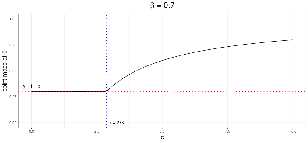
Figure 1. Illustration of the result of Theorem 4.23 as $c$ varies when $\beta=0.7$

Theorem 4.24.

Suppose $L(H_{n},H)\rightarrow 0$ where $H_{n},H$ are bi-variate distributions over $\mathbb{R}_{+}^{2}$ and $L(\cdot,\cdot)$ denotes the Levy distance. If $\exists K>0$ such that

(4.19) $$\underset{k=1,2}{\max}\bigg{\{}\underset{n\rightarrow\infty}{\limsup}\int_{\mathbb{R}_{+}^{2}}\lambda_{k}^{2}dH_{n}(\lambda_{1},\lambda_{2})\bigg{\}}<K$$

then, $\underset{n\rightarrow\infty}{\lim}\textbf{h}(z,H_{n})=\textbf{h}(z,H)$ for any $z\in\mathbb{C}_{L}$.

For the proof, please refer to Section E.4.

5. Special Case: Equal covariance matrices

Now we consider the special case where $\Sigma_{1n}=\Sigma_{n}=\Sigma_{2n}$. Here, Theorem 4.3 reduces to a simpler form and holds under weaker conditions. In this case, we replace Assumptions $T_{4}$ and $T_{5}$ of Theorem 4.3 with $T_{4}^{{}^{\prime}}$ and $T_{5}^{{}^{\prime}}$ respectively.

1. The ESD of $\Sigma_{n}$ converges weakly to a uni-variate probability distribution $H\neq\delta_{0}$ almost surely, i.e. $F^{\Sigma_{n}}\xrightarrow{d}H$ a.s. and $\operatorname{supp}(H)\subset\mathbb{R}_{+}$

2. Further, $\exists$ $C_{0}>0$ such that $\underset{n\rightarrow\infty}{\limsup}\frac{1}{p}\operatorname{trace}(\Sigma_{n})<C_{0}$

It is clear that Assumption $T_{5}^{{}^{\prime}}$ follows from Assumption $T_{5}$. To characterize the main result of this section, we need the uni-variate analog of the functions (4.1) that were integral to the main result of Section 4.

Definition 5.1.

Define the complex-valued functions $\sigma,\sigma_{2}$ as

(5.1) $$\sigma(z): =\frac{1}{\mathbbm{i}+z}+\frac{1}{-\mathbbm{i}+z}=\frac{2z}{1+z^{2}},z\not\in\{\mathbbm{i},-\mathbbm{i}\}$$

(5.2) $$\sigma_{2}(z): =\frac{1}{|\mathbbm{i}+z|^{2}}+\frac{1}{|-\mathbbm{i}+z|^{2}},z\not\in\{\mathbbm{i},-\mathbbm{i}\}$$

Then for $z\not\in\{\mathbbm{i},-\mathbbm{i}\}$ we have,

(5.3) $$\Re(\sigma(z)) =\frac{\Re(\overline{\mathbbm{i}+z})}{|\mathbbm{i}+z|^{2}}+\frac{\Re(\overline{-\mathbbm{i}+z})}{|-\mathbbm{i}+z|^{2}}=\sigma_{2}(z)\Re(z)$$

Corollary 5.2.

In Theorem 4.3, suppose we have $\Sigma_{1n}=\Sigma_{2n}=\Sigma_{n}$ for $n\in\mathbb{N}$ such that $F^{\Sigma_{n}}\xrightarrow{d}H$ a.s. where $H\neq\delta_{0}$ is a non-random uni-variate distribution on $\mathbb{R}_{+}$. Then under $T_{1},T_{2},T_{4}^{{}^{\prime}},T_{5}^{{}^{\prime}}$, we have $F^{S_{n}}\xrightarrow{d}F$ a.s. where $F$ is a non-random distribution with Stieltjes Transform at $z\in\mathbb{C}_{L}$ given by

(5.4) $$s(z)=\int\frac{dH(\lambda)}{-z+\lambda\sigma(ch(z))}=\dfrac{1}{z}\bigg{(}\dfrac{2}{c}-1\bigg{)}-\dfrac{2}{cz}\bigg{(}\dfrac{1}{1+c^{2}h^{2}(z)}\bigg{)}$$

where $h(z)\in\mathbb{C}_{R}$ is the unique number such that

(5.5) $$h(z)=\int\dfrac{\lambda dH(\lambda)}{-z+\lambda\sigma(ch(z)))}$$

Further $h$ is the Stieltjes Transform of a measure (not necessarily a probability) over the imaginary axis and has a continuous dependence on $H$.

Unlike in Section 4, when both covariance matrices are equal, the uniqueness and continuity (w.r.t the weak topology) of the solution of (4.5) can be proved without requiring any spectral moment bounds (i.e,4.7, 4.3) and/ or other technical conditions (4.19). Moreover, in the special case, the result regarding the continuity of the solution w.r.t. the weak topology is much stronger in the sense that it holds for any weakly converging sequence of distribution functions. Hence, to complete the proof of Corollary 5.2, we will prove the uniqueness and continuity of the solution of (5.5) without these extra conditions.

Theorem 5.3.

Uniqueness of solution when $\Sigma_{1n}=\Sigma_{n}=\Sigma_{2n}$: There exists at most one solution to the following equation within the class of functions that map $\mathbb{C}_{L}$ to $\mathbb{C}_{R}$.

$$h(z)=\int\dfrac{\lambda dH(\lambda)}{-z+\lambda\sigma(ch(z))}$$

where H is any probability distribution function such that $\operatorname{supp}(H)\subset\mathbb{R}_{+}$ and $H\neq\delta_{0}$.

The proof is given in Section F.1.

Theorem 5.4.

Continuity of solution when $\Sigma_{1n}=\Sigma_{n}=\Sigma_{2n}$: Let $H_{n},H$ be uni-variate distribution functions satisfying the conditions in Corollary 5.2 and $H_{n}\xrightarrow{d}H$. For a fixed $z\in\mathbb{C}_{L}$, denote the unique solutions to (5.5) corresponding to $H_{n}$ and $H$ as $h(z,H_{n})$ and $h(z,H)$ respectively. Then $h(z,H_{n})\xrightarrow{}h(z,H)$.

The proof is given in Section F.2.

6. LSD when the common covariance is the Identity Matrix

When $\Sigma_{n}=I_{p}$ a.s., we have $F^{\Sigma_{n}}=\delta_{1}$ for all $n\in\mathbb{N}$ and thus $F^{\Sigma_{n}}\xrightarrow{d}\delta_{1}$ a.s. So plugging in $H=\delta_{1}$ in Corollary 5.2, there exists a probability distribution function $F$ on the imaginary axis such that $F^{S_{n}}\xrightarrow{d}F$. The LSD $F$ is characterized by $(h,s_{F})$ with $h$ satisfying (5.5) with $H=\delta_{1}$ and $(h,s_{F})$ satisfies (5.4). We will shortly see that $F$ in this case becomes an explicit function of $c$. Therefore, we will henceforth refer to the LSD as $F_{c}$. The goal of this section is to recover closed form expressions for the distribution $F_{c}$.

We first note that $h(z)$, the unique solution to (5.5) with positive real part is the same as $s_{F_{c}}(z)$ in this case. This is shown below. Writing $h(z)$ as $h$ for simplicity, we have from (5.5)

(6.1) $$\frac{1}{h}=-z+\frac{2ch}{1+c^{2}h^{2}}$$

$$\implies c^{2}zh^{3}+(c^{2}-2c)h^{2}+zh+1=0$$

$$\implies c^{2}zh^{3}+zh=-1-h^{2}(c^{2}-2c)$$

$$\implies c^{3}zh^{3}+czh=-c-c^{2}h^{2}(c-2)$$

$$\implies czh(c^{2}h^{2}+1)=2-c+c^{2}h^{2}(2-c)-2=(2-c)(c^{2}h^{2}+1)-2$$

$$\implies czh=2-c-\frac{2}{1+c^{2}h^{2}}=2-c+\frac{1}{\mathbbm{i}}\bigg{(}\frac{1}{\mathbbm{i}+ch}-\frac{1}{-\mathbbm{i}+ch}\bigg{)}$$

$$\implies h=\frac{1}{z}\bigg{(}\frac{2}{c}-1\bigg{)}-\frac{2}{cz}\bigg{(}\frac{1}{1+c^{2}h^{2}}\bigg{)}=s_{F_{c}}(z)\text{, by }(\ref{s_main_eqn_1})$$

Therefore, the Stieltjes Transform ($s_{F_{c}}(z)$) of the LSD at $z\in\mathbb{C}_{L}$ can be recovered by finding the unique solution with positive real part (exactly one exists by Theorem 4.3) to the following equation.

(6.2) $$\frac{1}{m(z)}=-z+\frac{2cm(z)}{1+c^{2}m^{2}(z)}$$

We simplify (6.2) to an equivalent functional cubic equation which is more amenable for recovering the roots.

(6.3) $$c^{2}zm^{3}(z)+(c^{2}-2c)m^{2}(z)+zm(z)+1=0$$

For $z\in\mathbb{C}_{L}$, we extract the functional roots $\{m_{j}(z)\}_{j=1}^{3}$ of (6.3) using Cardano’s method (subsection 3.8.2 of [1]) and select the one which has a positive real component.

6.1. Deriving the functional roots

We define the following quantities as functions of $c\in(0,\infty)$.

(6.4) $$\left\{\begin{aligned} &q_{0}=\frac{1}{3c^{2}};\hskip 51.21495ptq_{2}=-\frac{(c-2)^{2}}{9c^{2}};\hskip 14.22636pt\tilde{q}=(q_{0},q_{2})\\ &r_{1}=-\frac{c+1}{3c^{3}};\hskip 34.1433ptr_{3}=-\frac{(c-2)^{3}}{27c^{3}};\hskip 14.22636pt\tilde{r}=(r_{1},r_{3})\\ &d_{0}=\dfrac{1}{27c^{6}};\hskip 48.36967ptd_{2}=\dfrac{2c^{2}+10c-1}{27c^{6}};\hskip 14.22636ptd_{4}=\dfrac{(c-2)^{3}}{27c^{5}};\hskip 14.22636pt\tilde{d}=(d_{0},d_{2},d_{4})\\ &Q(z):=q_{0}+\frac{q_{2}}{z^{2}};\hskip 19.91692ptR(z):=\frac{r_{1}}{z}+\frac{r_{3}}{z^{3}};z\in\mathbb{C}\backslash\{0\}\end{aligned}\right.$$

By Cardano’s method, the three roots of the cubic equation (6.3) are given as follows where $1,\omega_{1},\omega_{2}$ are the cube roots of unity.

(6.5) $$\left\{\begin{aligned} m_{1}(z)&=-\dfrac{1-2/c}{3z}+S_{0}+T_{0}\\ m_{2}(z)&=-\dfrac{1-2/c}{3z}+\omega_{1}S_{0}+\omega_{2}T_{0}\\ m_{3}(z)&=-\dfrac{1-2/c}{3z}+\omega_{2}S_{0}+\omega_{1}T_{0}\end{aligned}\right.$$

where $S_{0}$ and $T_{0}$ satisfy

(6.6) $$S_{0}^{3}+T_{0}^{3}=2R(z);\quad S_{0}T_{0}=-Q(z)$$

Note that if ($S_{0},T_{0}$) satisfy (6.6), then so do ($\omega_{1}S_{0},\omega_{2}T_{0}$) and ($\omega_{2}S_{0},\omega_{1}T_{0}$). But exactly one of the functional roots of (6.3) is the Stieltjes Transform $s_{F}(\cdot)$. This ambiguity in the definition of $S_{0}$ and $T_{0}$ prevents us from pinpointing which one among $\{m_{j}(z)\}_{j=1}^{3}$ is the Stieltjes transform of $F$ at $z$ unless we explicitly solve for the roots. However, we will show in Theorem 6.2 that at points arbitrarily close to the imaginary axis, it is possible to calculate the value of the Stieltjes transform thus allowing us to recover the distribution.

An interesting property of the roots of equation (6.3) can be found in Proposition G.4. We have also included a result regarding the continuity of the Stieltjes Transform ($s_{F_{c}}(\cdot)$) as a function of $c$ in Proposition G.5 and regarding the location of the Stieltjes Transform in Proposition G.6.

6.2. Deriving the density of the L.S.D

Certain properties of the LSD such as symmetry about $0$ and existence and value of point mass at $0$ have already been established in Proposition 4.21 and Theorem 4.23 respectively. Before deriving the density and support of the LSD $F_{c}$, we introduce a few quantities that parametrize said density.

Definition 6.1.

For $c>0$, let $\tilde{d},R(.),Q(.)$ be as in (6.4). Then define

1. $R_{\pm}:=\dfrac{d_{2}\pm\sqrt{d_{2}^{2}-4d_{0}d_{4}}}{2d_{0}};\hskip 14.22636pt$ $R_{\pm}$ are real numbers as shown in Lemma G.2

2. $L_{c}:=\sqrt{R_{-}\mathbbm{1}_{\{R_{-}>0\}}}$;    $U_{c}:=\sqrt{R_{+}}$

3. $S_{c}:=(-U_{c},-L_{c})\cup(L_{c},U_{c})$; It denotes the smallest open set excluding the point $0$ where the density of the LSD is finite.

4. For $x\neq 0$, let $r(x):=\underset{\epsilon\downarrow 0}{\lim}\hskip 2.84526ptR(-\epsilon+\mathbbm{i}x)$ and $q(x):=\underset{\epsilon\downarrow 0}{\lim}\hskip 2.84526ptQ(-\epsilon+\mathbbm{i}x)$
   Results related to these limits are established in Lemma G.2

5. For $x\neq 0$, $d(x):=d_{0}-\dfrac{d_{2}}{x^{2}}+\dfrac{d_{4}}{x^{4}}$

Theorem 6.2.

$F_{c}$ is differentiable at $x\neq 0$ for any $c>0$. Define $V_{\pm}(x):=|r(x)|\pm\sqrt{-d(x)}$. The functional form of the density is given by

$$f_{c}(x)=\dfrac{\sqrt{3}}{2\pi}\left((V_{+}(x))^{\frac{1}{3}}-(V_{-}(x))^{\frac{1}{3}}\right)\mathbbm{1}_{\{x\in S_{c}\}}$$

At $x=0$, the derivative exists only when $0<c<2$ and is given by

$$f_{c}(0)=\dfrac{1}{\pi\sqrt{2c-c^{2}}}$$

The density is continuous wherever it exists.

The proof can be found in Section G.2.

6.3. Simulation study

We ran simulations for different values of $c$ while keeping $p=2000$. Data matrices (i.e., $Z_{1},Z_{2}$) were generated with independent observations, a random half of which were simulated from $\mathcal{N}(0,1)$ and the other half from $\mathcal{U}(-\sqrt{3},\sqrt{3}$). Figures 2(a), 2(b), 2(c), 2(d) 2(e) and 2(f) below show the comparison of the ESDs of these matrices for different against the theoretical distribution from Theorem 6.2. We have also run these simulations for smaller values of $p$ such as $p=750$. The results are visually similar to the ones provided below.

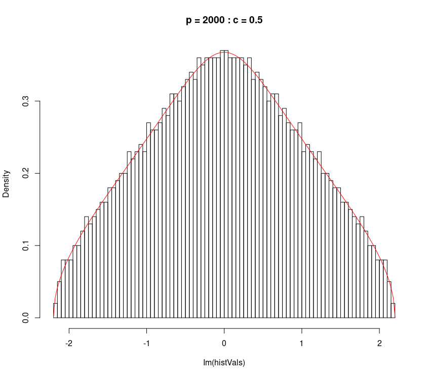
(a) c=0.5

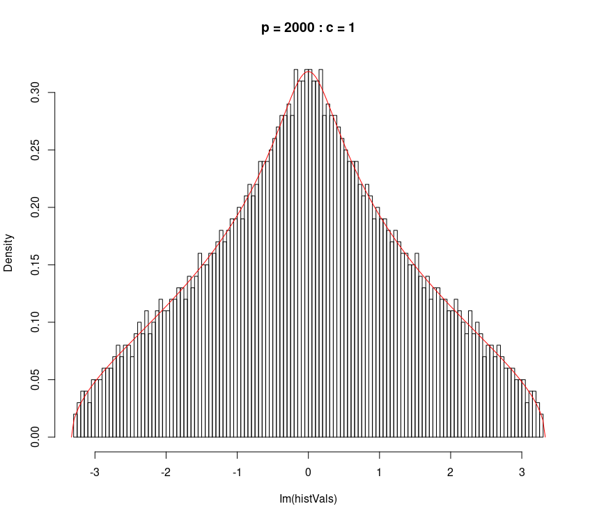
(b) c=1

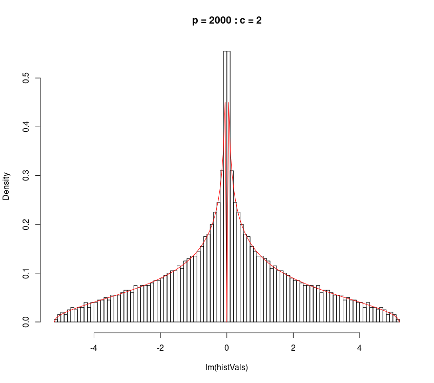
(c) c=2

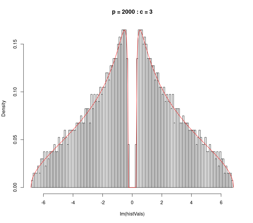
(d) c=3

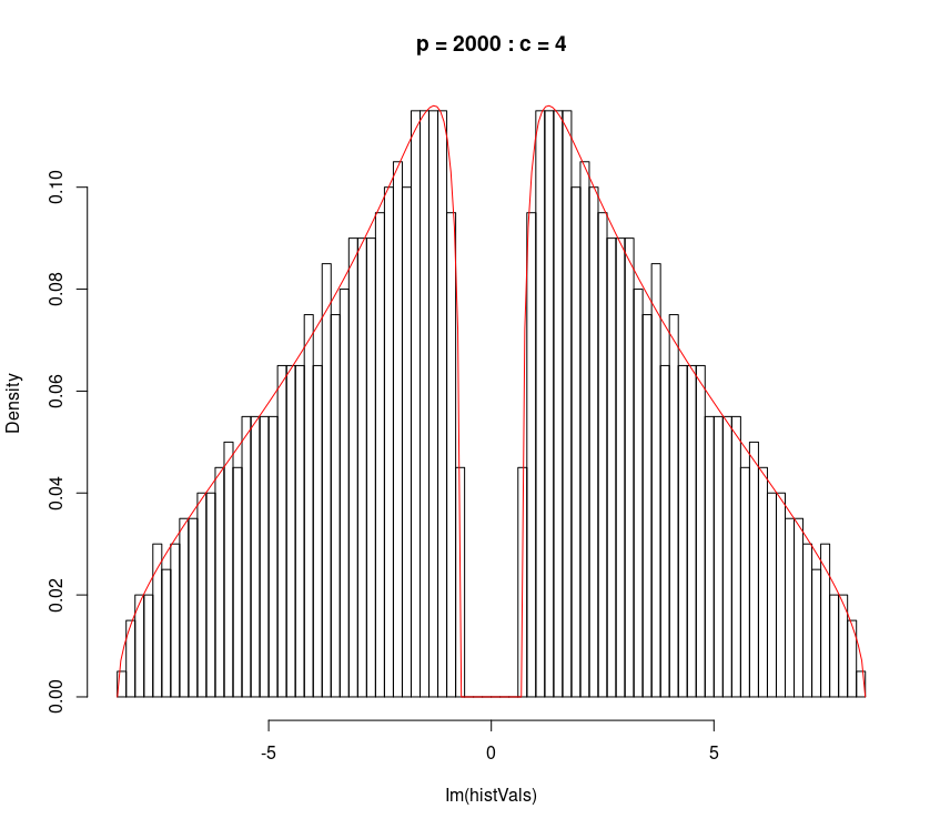
(e) c=4

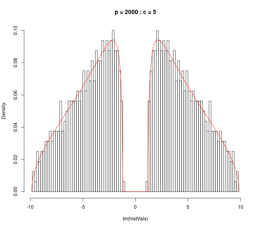
(f) c=5

Figure 2. Simulated vs. theoretical limit distributions at various levels of $c$ for $\Sigma_{n}=I_{p}$

7. The case of the Anti-Commutator Matrix

We define the anti-commutator matrix of $X_{1},X_{2}$ as

(7.1) $$S_{n}^{+}=\frac{1}{n}(X_{1}X_{2}^{*}+X_{2}X_{1}^{*})=\frac{1}{n}\{X_{1},X_{2}\}$$

Note that

(7.2) $$\frac{1}{n}[X_{1},\mathbbm{i}X_{2}]=\frac{1}{n}(X_{1}(\mathbbm{i}X_{2})^{*}-\mathbbm{i}X_{2}X_{1}^{*})=-\frac{1}{n}\mathbbm{i}(X_{1}X_{2}^{*}+X_{2}X_{1}^{*})=-\frac{\mathbbm{i}}{n}\{X_{1},X_{2}\}$$

This in particular implies that the LSD of the anti-commutator of $X_{1}$ and $\mathbbm{i}X_{2}$ is the same as that of the commutator of $X_{1}$ and $X_{2}$ upon counter-clockwise rotation by $\pi/2$. Noting that $X_{2}$ and $\mathbbm{i}X_{2}$ both satisfy Assumption $T_{1}$ in Theorem 4.3, we have the following result.

Corollary 7.1.

Under ($T_{1}-T_{5}$) of Theorem 4.3, $F^{S_{n}^{+}}\xrightarrow{d}G$ where the Stieltjes Transform of G at $z\in\mathbb{C}^{+}$ is characterized by the set of equations.

(7.3) $$s_{G}(z)=\displaystyle\int_{\mathbb{R}_{+}^{2}}\frac{dH(\boldsymbol{\lambda})}{-z-\mathbbm{i}\boldsymbol{\lambda}^{T}\boldsymbol{\rho}(c\textbf{h}(\mathbbm{i}z))}=\frac{1}{z}\bigg{(}\frac{2}{c}-1\bigg{)}-\frac{2}{cz}\bigg{(}\frac{1}{1+c^{2}h_{1}(\mathbbm{i}z)h_{2}(\mathbbm{i}z)}\bigg{)}$$

where $\textbf{h}(\mathbbm{i}z)=(h_{1}(\mathbbm{i}z),h_{2}(\mathbbm{i}z))^{T}\in\mathbb{C}_{R}^{2}$ are unique numbers such that

(7.4) $$\mathbbm{i}\textbf{h}(\mathbbm{i}z) =\displaystyle\int_{\mathbb{R}_{+}^{2}}\frac{\boldsymbol{\lambda}dH(\boldsymbol{\lambda})}{-z-\mathbbm{i}\boldsymbol{\lambda}^{T}\boldsymbol{\rho}(c\textbf{h}(\mathbbm{i}z))}$$

Moreover, $h_{1},h_{2}$ themselves are Stieltjes Transforms of measures (not necessarily probability measures) over the imaginary axis and continuous as functions of $H$.

Proof.

The proof is immediate from (7.2) and Lemma 3.4. ∎

Acknowledgments: The authors would like to thank Professor Arup Bose for some insightful suggestions and discussions.

Appendix A A few general results

A.1. A few basic results related to matrices

• Resolvent identity: $A^{-1}-B^{-1}=A^{-1}(B-A)B^{-1}=B^{-1}(B-A)A^{-1}$

• For skew-Hermitian matrices $A,B\in\mathbb{C}^{p\times p}$, we have

  (A.1) $$||F^{A}-F^{B}||_{im}=||F^{-\mathbbm{i}A}-F^{-\mathbbm{i}B}||\leq\frac{1}{p}\operatorname{rank}(A-B)$$

  The first equality follows from (2.2) and the last inequality follows from Lemma 2.4 of [21].

• For a rectangular matrix, we have $\operatorname{rank}(A)\leq$ the number of non-zero entries of A. This is a result from Lemma 2.1 of [21].

• $\operatorname{rank}(AXB-PXQ)\leq\operatorname{rank}(A-P)+\operatorname{rank}(B-Q)$ where the dimensions of relevant matrices are compatible

• Cauchy-Schwarz Inequality: $|a^{*}Xb|\leq||X||_{op}\,||a||\,||b||$

• For a p.s.d. matrix B and any square matrix A, $|\operatorname{trace}(AB)|\leq||A||_{op}\operatorname{trace}(B)$.

• For $A,B\in\mathbb{R}^{N\times N}$, $|\operatorname{trace}(AB)|\leq N||A||_{op}\,||B||_{op}$

Lemma A.1.

Let $\{F_{n},G_{n}\}_{n=1}^{\infty}$ be sequences of distribution functions on $\mathbbm{i}\mathbb{R}$ with $s_{F_{n}}(z),s_{G_{n}}(z)$ denoting their respective Stieltjes transforms at $z\in\mathbb{C}_{L}$. If $L_{im}(F_{n},G_{n})\rightarrow 0$, then $|s_{F_{n}}(z)-s_{G_{n}}(z)|\rightarrow 0$.

Proof.

As usual, for a distribution function $F$ on $\mathbbm{i}\mathbb{R}$, we denote its real counterpart as $\overline{F}$. Let $\mathcal{P}(\mathbb{R})$ represent the set of all probability distribution functions on $\mathbb{R}$. Then the bounded Lipschitz metric is defined as follows

$$\beta:\mathcal{P}(\mathbb{R})\times\mathcal{P}(\mathbb{R})\rightarrow\mathbb{R}_{+}\text{, where }\beta(\overline{F},\overline{G}):=\underset{}{\sup}\bigg{\{}\bigg{|}\int hd\overline{F}-\int hd\overline{G}\bigg{|}:||h||_{BL}\leq 1\bigg{\}}$$

$$\text{and }||h||_{BL}=\sup\{|h(x)|:x\in\mathbb{R}\}+\underset{x\neq y}{\sup}\dfrac{|h(x)-h(y)|}{|x-y|}$$

From Corollary 18.4 and Theorem 8.3 of [10], we have the following relationship between Levy (L) and bounded Lipschitz ($\beta$) metrics.

(A.2) $$\frac{1}{2}\beta(\overline{F},\overline{G})\leq L(\overline{F},\overline{G})\leq 3\sqrt{\beta(\overline{F},\overline{G})}$$

Fix $z\in\mathbb{C}_{L}$ arbitrarily. Define $g_{z}(x):=(\mathbbm{i}x-z)^{-1}$. Note that, $|g_{z}(x)|\leq 1/|\Re(z)|$ $\forall x\in\mathbb{R}$. Also,

$$|g_{z}(x_{1})-g_{z}(x_{2})|=\bigg{|}\frac{1}{\mathbbm{i}x_{1}-z}-\frac{1}{\mathbbm{i}x_{2}-z}\bigg{|}=\frac{|x_{1}-x_{2}|}{|\mathbbm{i}x_{1}-z||\mathbbm{i}x_{2}-z|}\leq|x_{1}-x_{2}|\frac{1}{\Re^{2}(z)}$$

Note that $||g_{z}||_{BL}\leq{1}/{|\Re(z)|}+{1}/{\Re^{2}(z)}<\infty$. Then for $g:={g_{z}}/{||g_{z}||_{BL}}$, we have $||g||_{BL}=1$.

By (A.2) and (3.4) and using $dF_{n}(\mathbbm{i}x)=d\overline{F}_{n}(x)$ for $x\in\mathbb{R}$, we have

$$L_{im}(F_{n},G_{n})\rightarrow 0\leftrightarrow L(\overline{F}_{n},\overline{G}_{n})\rightarrow 0$$

$$\leftrightarrow \beta(\overline{F}_{n},\overline{G}_{n})\rightarrow 0$$

$$\implies \bigg{|}\int_{\mathbb{R}}g(x)d\overline{F}_{n}(x)-\int_{\mathbb{R}}g(x)d\overline{G}_{n}(x)\bigg{|}\rightarrow 0$$

$$\implies \bigg{|}\int_{\mathbb{R}}\frac{1}{\mathbbm{i}x-z}dF_{n}(\mathbbm{i}x)-\int_{\mathbb{R}}\frac{1}{\mathbbm{i}x-z}dG_{n}(\mathbbm{i}x)\bigg{|}\rightarrow 0$$

$$\implies |s_{F_{n}}(z)-s_{G_{n}}(z)|\longrightarrow 0$$

∎

Lemma A.2.

Let $\{X_{jn},Y_{jn}:1\leq j\leq n\}_{n=1}^{\infty}$ be triangular arrays of random variables. Suppose $\underset{1\leq j\leq n}{\max}|X_{jn}|\xrightarrow{a.s.}0$ and $\underset{1\leq j\leq n}{\max}|Y_{jn}|\xrightarrow{a.s.}0$. Then $\underset{1\leq j\leq n}{\max}|X_{jn}+Y_{jn}|\xrightarrow{a.s.}0$.

Proof.

Let $A_{x}:=\{\omega:\underset{n\rightarrow\infty}{\lim}\underset{1\leq j\leq n}{\max}|X_{jn}(\omega)|=0\}$, $A_{y}:=\{\omega:\underset{n\rightarrow\infty}{\lim}\underset{1\leq j\leq n}{\max}|Y_{jn}(\omega)|=0\}$. Then $\mathbb{P}(A_{x})=1=\mathbb{P}(A_{y})$. Then $\forall\omega\in A_{x}\cap A_{y}$, we have $0\leq|X_{jn}(\omega)+Y_{jn}(\omega)|\leq|X_{jn}(\omega)|+|Y_{jn}(\omega)|$. Hence, $\underset{n\rightarrow\infty}{\lim}\underset{1\leq j\leq n}{\max}|X_{jn}(\omega)+Y_{jn}(\omega)|=0$. But, $\mathbb{P}(A_{x}\cap A_{y})=1$. Therefore, the result follows. ∎

Lemma A.3.

Let $\{A_{jn},B_{jn},C_{jn},D_{jn}:1\leq j\leq n\}_{n=1}^{\infty}$ be triangular arrays of random variables. Suppose $\underset{1\leq j\leq n}{\max}|A_{jn}-C_{jn}|\xrightarrow{a.s.}0$ and $\underset{1\leq j\leq n}{\max}|B_{jn}-D_{jn}|\xrightarrow{a.s.}0$ and $\exists N_{0}\in\mathbb{N}$ such that $|C_{jn}|\leq B_{1}$ a.s. and $|D_{jn}|\leq B_{2}$ a.s. when $n>N_{0}$ for some $B_{1},B_{2}\geq 0$. Then $\underset{1\leq j\leq n}{\max}|A_{jn}B_{jn}-C_{jn}D_{jn}|\xrightarrow{a.s.}0$.

Proof.

Let $\Omega_{1}=\{\omega:\underset{n\rightarrow\infty}{\lim}\underset{1\leq j\leq n}{\max}|A_{jn}(\omega)-C_{jn}(\omega)|=0\}$, $\Omega_{2}=\{\omega:\underset{n\rightarrow\infty}{\lim}\underset{1\leq j\leq n}{\max}|B_{jn}(\omega)-D_{jn}(\omega)|=0\}$, $\Omega_{3}=\{\omega:|C_{jn}(\omega)|\leq B_{1}\text{ for }n>N_{0}\}$ and $\Omega_{4}=\{\omega:|D_{jn}(\omega)|\leq B_{2}\text{ for }n>N_{0}\}$. Then $\Omega_{0}=\cap_{j=1}^{4}\Omega_{j}$ is a set of probability $1$. Then $\forall\omega\in\Omega_{0}$, $\underset{1\leq j\leq n}{\max}|B_{jn}(\omega)|\leq B_{2}$ eventually for large $n$. Therefore for $\omega\in\Omega_{0}$ and large $n$, we get the following that concludes the proof.

$$\underset{1\leq j\leq n}{\max}|A_{jn}B_{jn}-C_{jn}D_{jn}| \leq\underset{1\leq j\leq n}{\max}|A_{jn}-C_{jn}||B_{jn}|+\underset{1\leq j\leq n}{\max}|C_{jn}||B_{jn}-D_{jn}|$$

$$\leq B_{2}\underset{1\leq j\leq n}{\max}|A_{jn}-C_{jn}|+B_{1}\underset{1\leq j\leq n}{\max}|B_{jn}-D_{jn}|\xrightarrow{a.s.}0$$

∎

Lemma A.4.

Let $\{X_{jn},Y_{jn}:1\leq j\leq n\}_{n=1}^{\infty}$ be triangular arrays of random variables such that $\underset{1\leq j\leq n}{\max}|X_{jn}-Y_{jn}|\xrightarrow{a.s.}0$. Then $|\frac{1}{n}\sum_{j=1}^{n}(X_{jn}-Y_{jn})|\xrightarrow{a.s.}0$.

Proof.

Let $M_{n}:=\underset{1\leq j\leq n}{\max}|X_{jn}-Y_{jn}|$. We have $|\frac{1}{n}\sum_{j=1}^{n}(X_{jn}-Y_{jn})|\leq\frac{1}{n}\sum_{j=1}^{n}|X_{jn}-Y_{jn}|\leq M_{n}$. Let $\epsilon>0$ be arbitrary. Then $\exists\Omega_{0}\subset\Omega$ such that $\mathbb{P}(\Omega_{0})=1$ and $\forall\omega\in\Omega_{0}$, we have $M_{n}(\omega)<\epsilon$ for sufficiently large $n\in\mathbb{N}$. Then, $\mathbb{P}(\{\omega:|\frac{1}{n}\sum_{j=1}^{n}(X_{jn}-Y_{jn})|<\epsilon\})=1$. Since $\epsilon>0$ is arbitrary, the result follows. ∎

We state the following result (Lemma B.26 of [2]) without proof.

Lemma A.5.

Let $A=(a_{ij})$ be an $n\times n$ non-random matrix and $x=(x_{1},\ldots,x_{n})^{T}$ be a vector of independent entries. Suppose $\mathbb{E}x_{i}=0,\mathbb{E}|x_{i}|^{2}=1$, and $\mathbb{E}|x_{i}|^{l}\leq\nu_{l}$. Then for $k\geq 1$, $\exists$ $C_{k}>0$ independent of $n$ such that

$$\mathbb{E}|x^{*}Ax-\operatorname{trace}(A)|^{k}\leq C_{k}\bigg{(}(\nu_{4}\operatorname{trace}(AA^{*}))^{\frac{k}{2}}+\nu_{2k}\operatorname{trace}\{(AA^{*})^{\frac{k}{2}}\}\bigg{)}$$

Simplification: For deterministic matrix $A$ with $||A||_{op}<\infty$, let $B=\frac{A}{||A||_{op}}$. Then $||B||_{op}=1$ and by $R_{6}$ of A.1, $\operatorname{trace}(BB^{*})\leq n||B||_{op}^{2}=n$ and $\operatorname{trace}\{(BB^{*})^{\frac{k}{2}}\}\leq n||B||_{op}^{k}=n$. Then by Lemma A.2, we have

(A.3) $$\mathbb{E}|x^{*}Bx-\operatorname{trace}(B)|^{k}\leq C_{k}\bigg{(}(\nu_{4}\operatorname{trace}(BB^{*}))^{\frac{k}{2}}+\nu_{2k}\operatorname{trace}\{(BB^{*})^{\frac{k}{2}}\}\bigg{)}$$

$$\implies \frac{\mathbb{E}|x^{*}Ax-\operatorname{trace}(A)|^{k}}{||A||_{op}^{k}}\leq C_{k}[(n\nu_{4})^{\frac{k}{2}}+n\nu_{2k}]$$

$$\implies \mathbb{E}|x^{*}Ax-\operatorname{trace}(A)|^{k}\leq C_{k}||A||_{op}^{k}[(n\nu_{4})^{\frac{k}{2}}+n\nu_{2k}]$$

We will be using this form of the inequality going forward.

Lemma A.6.

Let $\{x_{jn}:1\leq j\leq n\}_{n=1}^{\infty}$ be a triangular array of complex valued random vectors in $\mathbb{C}^{p}$ with independent entries. For $1\leq r\leq n$, denote the $r^{th}$ element of $x_{jn}$ as $x_{jn}^{(r)}$. Suppose $\mathbb{E}x_{jn}^{(r)}=0,\mathbb{E}|x_{jn}^{(r)}|^{2}=1$ and for $k\geq 1$, $\nu_{k}:=\mathbb{E}|x_{jn}^{(r)}|^{k}\leq n^{ak}$ where $0<a<\frac{1}{4}$. Suppose $A_{j}\in\mathbb{C}^{p\times p}$ is independent of $x_{jn}$ and $||A_{j}||_{op}\leq B$ a.s. for some $B>0$. Then,

$$\underset{1\leq j\leq n}{\max}\left|\dfrac{1}{n}x_{jn}^{*}Ax_{jn}-\dfrac{1}{n}\operatorname{trace}(A_{j})\right|\xrightarrow{a.s}0$$

Proof.

For arbitrary $\epsilon>0$ and $k\geq 1$, we have

$$p_{n}:= \mathbb{P}\bigg{(}\underset{1\leq j\leq n}{\max}\left|\dfrac{1}{n}x_{jn}^{*}A_{j}x_{jn}-\dfrac{1}{n}\operatorname{trace}(A_{j})\right|>\epsilon\bigg{)}$$

$$\leq\sum_{j=1}^{n}\mathbb{P}\bigg{(}\left|\dfrac{1}{n}x_{jn}^{*}A_{j}x_{jn}-\dfrac{1}{n}\operatorname{trace}(A_{j})\right|>\epsilon\bigg{)}\text{, by union bound}$$

$$\leq\sum_{j=1}^{n}\dfrac{\mathbb{E}\left|\dfrac{1}{n}x_{jn}^{*}A_{j}x_{jn}-\dfrac{1}{n}\operatorname{trace}(A_{j})\right|^{k}}{\epsilon^{k}}\text{, for any }k\in\mathbb{N}$$

$$= \sum_{j=1}^{n}\dfrac{\mathbb{E}\bigg{(}\mathbb{E}\bigg{[}|\dfrac{1}{n}x_{jn}^{*}A_{j}x_{jn}-\dfrac{1}{n}\operatorname{trace}(A_{j})|^{k}\bigg{|}A_{j}\bigg{]}\bigg{)}}{\epsilon^{k}}$$

$$\leq\sum_{j=1}^{n}\dfrac{\mathbb{E}||A_{j}||_{op}^{k}C_{k}((n\nu_{4})^{\frac{k}{2}}+n\nu_{2k})}{n^{k}\epsilon^{k}}\text{ by }(\ref{I1})$$

$$\leq\sum_{j=1}^{n}\dfrac{K[(n^{1+4a})^{\frac{k}{2}}+n^{1+2ak}]}{n^{k}}\text{, where }K=C_{k}\bigg{(}\frac{B}{\epsilon}\bigg{)}^{k}$$

$$=\dfrac{nK[n^{\frac{k}{2}+2ak}+n^{1+2ak}]}{n^{k}}=\frac{K}{n^{k(\frac{1}{2}-2a)-1}}+\frac{K}{n^{k(1-2a)-2}}$$

Since $0<a<\frac{1}{4}$, we can choose $k\in\mathbb{N}$ large enough so that $\min\{k(\frac{1}{2}-2a)-1,k(1-2a)-2\}>1$ to ensure that $\sum_{n=1}^{\infty}p_{n}$ converges. Therefore by Borel Cantelli lemma we have the result. ∎

Corollary A.7.

Let $\{u_{jn},v_{jn}:1\leq j\leq n\}_{n=1}^{\infty}$ be triangular arrays and $A_{j}$ be complex matrices as in Lemma A.6 with $u_{jn}$ and $v_{jn}$ independent of each other. Then,

$$\underset{1\leq j\leq n}{\max}\left|\frac{1}{n}u_{jn}^{*}A_{j}v_{jn}\right|\xrightarrow{a.s.}0$$

Proof.

Let $Q_{j}(u,v):=\frac{1}{n}u_{jn}^{*}A_{j}v_{jn}$. Define $Q_{j}(v,v),Q_{j}(u,u),Q_{j}(v,u)$ similarly. Let $x_{jn}=\frac{1}{\sqrt{2}}(u_{jn}+v_{jn})$. Now applying Lemma A.6, we get

(A.4) $$\underset{1\leq j\leq n}{\max}\left|\frac{1}{n}x_{jn}^{*}A_{j}x_{jn}-\frac{1}{n}\operatorname{trace}(A_{j})\right|\xrightarrow{a.s.}0$$

$$\implies\underset{1\leq j\leq n}{\max}\left|\frac{1}{2}(Q_{j}(u,u)-T_{j})+\frac{1}{2}(Q_{j}(v,v)-T_{j})+\frac{1}{2}(Q_{j}(u,v)+Q_{j}(v,u))\right|\xrightarrow{a.s.}0\text{, where }T_{j}:=\frac{1}{n}\operatorname{trace}(A_{j})$$

Now setting $x_{jn}=\frac{1}{\sqrt{2}}(u_{jn}+\mathbbm{i}v_{jn})$ and applying Lemma A.6, we get

(A.5) $$\underset{1\leq j\leq n}{\max}\left|\frac{1}{n}x_{jn}^{*}A_{j}x_{jn}-\frac{1}{n}\operatorname{trace}(A_{j})\right|\xrightarrow{a.s.}0$$

$$\implies\underset{1\leq j\leq n}{\max}\left|\frac{1}{2}(Q_{j}(u,u)-T_{j})+\frac{1}{2}(Q_{j}(v,v)-T_{j})+\frac{1}{2}\mathbbm{i}(Q_{j}(u,v)-Q_{j}(v,u))\right|\xrightarrow{a.s.}0$$

Using Lemma A.2 on (A.4) and (A.5), we get $\underset{1\leq j\leq n}{\max}|Q_{j}(u,v)|\xrightarrow{a.s.}0$. ∎

Lemma A.8.

2-rank perturbation equality: Let $B\in\mathbb{C}^{p\times p}$ be of the form $B=A-zI_{p}$ for some skew-Hermitian matrix $A$ and $z\in\mathbb{C}_{L}$. For vectors $u,v\in\mathbb{C}^{p}$, define $\langle u,v\rangle:=u^{*}B^{-1}v$. Then,

1:

$(B+uv^{*}-vu^{*})^{-1}u=B^{-1}(\alpha_{1}u+\beta_{1}v)$; $\alpha_{1}=(1-\langle u,v\rangle)D(u,v)$; $\beta_{1}=\langle u,u\rangle D(u,v)$

2:

$(B+uv^{*}-vu^{*})^{-1}v=B^{-1}(\alpha_{2}v+\beta_{2}u)$; $\alpha_{2}=(1+\langle v,u\rangle)D(u,v)$; $\beta_{2}=-\langle v,v\rangle D(u,v)$

where $D(u,v)=\bigg{(}(1-\langle u,v\rangle)(1+\langle v,u\rangle)+\langle u,u\rangle\langle v,v\rangle\bigg{)}^{-1}$

Proof.

Clearly, $B$ cannot have zero as eigenvalue. So $\langle u,v\rangle$ is well defined. For $P\in\mathbb{C}^{p\times p},Q,R\in\mathbb{C}^{p\times n}$ with $P+QR^{*}$ and $P$ being invertible, Woodbury’s formula states that

(A.6) $$(P+QR^{*})^{-1} =P^{-1}-P^{-1}Q(I_{n}+R^{*}P^{-1}Q)^{-1}R^{*}P^{-1}$$

(A.7) $$\implies(P+QR^{*})^{-1}Q =P^{-1}Q-P^{-1}Q(I_{n}+R^{*}P^{-1}Q)^{-1}R^{*}P^{-1}Q$$

$$=P^{-1}Q\bigg{(}I_{n}-(I_{n}+R^{*}P^{-1}Q)^{-1}R^{*}P^{-1}Q\bigg{)}$$

Let $P=B$, $Q=[u:v]$ and $R=[v:-u]$. Note that $\operatorname{det}(I_{2}+R^{*}P^{-1}Q)^{-1}=D(u,v)$. So, $D(u,v)$ is well-defined. Finally, observing that $B+uv^{*}-vu^{*}=P+QR^{*}$, we use (A.6) to get

$$(B+uv^{*}-vu^{*})^{-1}[u:v]$$

$$=B^{-1}[u:v]\bigg{(}I_{2}-(I_{2}+R^{*}P^{-1}Q)^{-1}R^{*}P^{-1}Q\bigg{)}$$

$$=B^{-1}[u:v]\bigg{(}I_{2}-{\begin{bmatrix}1+\langle v,u\rangle&\langle v,v\rangle\\ -\langle u,u\rangle&1-\langle u,v\rangle\end{bmatrix}}^{-1}\begin{bmatrix}\langle v,u\rangle&\langle v,v\rangle\\ -\langle u,u\rangle&-\langle u,v\rangle\\ \end{bmatrix}\bigg{)}$$

$$=B^{-1}[u:v]\bigg{(}I_{2}-D(u,v)\begin{bmatrix}1-\langle u,v\rangle&-\langle v,v\rangle\\ \langle u,u\rangle&1+\langle v,u\rangle\end{bmatrix}\begin{bmatrix}\langle v,u\rangle&\langle v,v\rangle\\ -\langle u,u\rangle&-\langle u,v\rangle\\ \end{bmatrix}\bigg{)}$$

$$=D(u,v)B^{-1}[u:v]\begin{bmatrix}\alpha_{1}&\beta_{2}\\ \beta_{1}&\alpha_{2}\end{bmatrix}$$

∎

Appendix B Intermediate Results

B.1. Results related to proof of uniqueness in (4.5)

Definition B.1.

For $\textbf{h}=(h_{1},h_{2})\in\mathbb{C}_{R}^{2}$ and $r,s\in\mathbb{N}\cup\{0\}$, we define $I_{r,s}(\textbf{h}(z),H):=\displaystyle\int\frac{\lambda_{1}^{r}\lambda_{2}^{s}dH(\boldsymbol{\lambda})}{|-z+\boldsymbol{\lambda}^{T}\boldsymbol{\rho}(c\textbf{h})|^{2}}$

Fix $z=-u+\mathbbm{i}v\in\mathbb{C}_{L}$ with $u>0$. Suppose $\textbf{h}=(h_{1},h_{2})$ satisfy (4.5). Then, with the above definition we observe that,

$$\Re(h_{1}) =\int\frac{\lambda_{1}\Re(\overline{-z+\boldsymbol{\lambda}^{T}\boldsymbol{\rho}(c\textbf{h}))}}{|-z+\boldsymbol{\lambda}^{T}\boldsymbol{\rho}(c\textbf{h})|^{2}}dH(\boldsymbol{\lambda})$$

$$=u\int\frac{\lambda_{1}dH(\boldsymbol{\lambda})}{|-z+\boldsymbol{\lambda}^{T}\boldsymbol{\rho}(c\textbf{h})|^{2}}+\Re(\rho_{1}(c\textbf{h}))\int\frac{\lambda_{1}^{2}dH(\boldsymbol{\lambda})}{|-z+\boldsymbol{\lambda}^{T}\boldsymbol{\rho}(c\textbf{h})|^{2}}+\Re(\rho_{2}(c\textbf{h}))\int\frac{\lambda_{1}\lambda_{2}dH(\boldsymbol{\lambda})}{|-z+\boldsymbol{\lambda}^{T}\boldsymbol{\rho}(c\textbf{h})|^{2}}$$

(B.1) $$=uI_{1,0}(\textbf{h},H)+\Re(\rho_{1}(c\textbf{h}))I_{2,0}(\textbf{h},H)+\Re(\rho_{2}(c\textbf{h}))I_{1,1}(\textbf{h},H)$$

Similarly we get

(B.2) $$\Re(h_{2}) =uI_{0,1}(\textbf{h},H)+\Re(\rho_{1}(ch))I_{1,1}(\textbf{h},H)+\Re(\rho_{2}(ch))I_{0,2}(\textbf{h},H)$$

$$\Im(h_{1}) =uI_{1,0}(\textbf{h},H)-\Im(\rho_{1}(ch))I_{2,0}(\textbf{h},H)-\Im(\rho_{2}(ch))I_{1,1}(\textbf{h},H)$$

$$\Im(h_{2}) =uI_{0,1}(\textbf{h},H)+\Im(\rho_{1}(ch))I_{1,1}(\textbf{h},H)-\Im(\rho_{2}(ch))I_{0,2}(\textbf{h},H)$$

Lemma B.2.

(Lipschitz within an isosceles sector): Recall the definition of $\mathcal{S}(b)$ from (4.10). For $0<b$, the functions $\rho_{1},\rho_{2}$ are Lipschitz continuous on $\mathcal{S}(b)^{2}=\mathcal{S}(b)\times\mathcal{S}(b)$.

Proof.

Let $\textbf{h}=(h_{1},h_{2}),\textbf{g}=(g_{1},g_{2})\in\mathcal{S}(b)^{2}$. First we establish a bound for $|1+h_{1}h_{2}|^{-1}$ and $|1+g_{1}g_{2}|^{-1}$. Clearly $\Re(h_{1}h_{2})\geq 0$ and therefore,

(B.3) $$\frac{1}{|1+h_{1}h_{2}|}=\frac{1}{\sqrt{(1+\Re(h_{1}h_{2}))^{2}+\Im^{2}(h_{1}h_{2})}}\leq 1$$

and the same bound works for $|1+g_{1}g_{2}|^{-1}$ as well.

We have

(B.4) $$|\rho_{1}(\textbf{h})|=|\rho_{1}(h_{1},h_{2})|=\left|\frac{h_{2}}{1+h_{1}h_{2}}\right|\leq b$$

We therefore have

$$\left|\rho_{1}(\textbf{h})-\rho_{1}(\textbf{g})\right| =\left|\frac{h_{2}}{1+h_{1}h_{2}}-\frac{g_{2}}{1+g_{1}g_{2}}\right|$$

$$=\left|\frac{(h_{2}-g_{2})+h_{2}g_{2}(g_{1}-h_{1})}{(1+h_{1}h_{2})(1+g_{1}g_{2})}\right|$$

$$\leq\left|\frac{h_{2}-g_{2}}{(1+h_{1}h_{2})(1+g_{1}g_{2})}\right|+|\rho_{1}(\textbf{h})||\rho_{1}(\textbf{g})|g_{1}-h_{1}|$$

$$\leq|h_{2}-g_{2}|+b^{2}|h_{1}-g_{1}|$$

$$\leq K_{0}||\textbf{h}-\textbf{g}||_{1}\text{, where }K_{0}:=\max\{1,b^{2}\}$$

∎

B.1.1. Proof of Lemma 4.10

Proof.

Note that $\boldsymbol{\rho}(c\textbf{h})\in\mathbb{C}_{R}^{2}$ follows from Remark 4.2. Therefore, for $\boldsymbol{\lambda}\in\mathbb{R}_{+}^{2}$,

(B.5) $$|-z+\boldsymbol{\lambda}^{T}\boldsymbol{\rho}(c\textbf{h})|\geq|u+\lambda_{1}\Re(\rho_{1}(c\textbf{h}))+\lambda_{2}\Re(\rho_{2}(c\textbf{h}))|\geq u$$

Therefore using (4.8), we have

(B.6) $$|h_{k}(z)|\leq\int\left|\frac{\lambda_{k}}{-z+\boldsymbol{\lambda}^{T}\boldsymbol{\rho}(c\textbf{h})}\right|dH(\boldsymbol{\lambda})\leq\int\frac{\lambda_{k}dH(\boldsymbol{\lambda})}{u}\leq\frac{C_{0}}{u}$$

For arbitrary $\epsilon>0$, there exist $\delta(\epsilon)>0$ such that $|\theta_{1}|,|\theta_{2}|<\delta(\epsilon)\implies|\rho_{k}(\theta_{1},\theta_{2})|<\epsilon$. Without loss of any generality, we can choose $\delta(\epsilon)<1$. By choosing $u>cC_{0}/\delta(\epsilon)$, we can ensure that $|ch_{k}(z)|<\delta(\epsilon)$. Then for such $z$, we have for $k=1,2$

(B.7) $$|\rho_{k}(c\textbf{h})|=|\rho_{k}(ch_{1},ch_{2})|<\epsilon$$

Now by (B.1), we have

(B.8) $$\Re(h_{1}(z)) =\,uI_{1,0}(\textbf{h},H)+\Re(\rho_{1}(c\textbf{h}))I_{2,0}(\textbf{h},H)+\Re(\rho_{2}(c\textbf{h}))I_{1,1}(\textbf{h},H)$$

(B.9) $$\Im(h_{1}(z)) =\,vI_{1,0}(\textbf{h},H)-\Im(\rho_{1}(c\textbf{h}))I_{2,0}(\textbf{h},H)-\Im(\rho_{2}(c\textbf{h}))I_{1,1}(\textbf{h},H)$$

First of all note that $I_{1,1}(\textbf{h},H)\leq\sqrt{I_{2,0}(\textbf{h},H)I_{0,2}(\textbf{h},H)}$ is immediate from the Cauchy-Schwarz inequality. Using $T_{5}$ of Theorem 4.3, we observe that

(B.10) $$I_{2,0}(\textbf{h},H)=\int\frac{\lambda_{1}^{2}dH(\boldsymbol{\lambda})}{|-z+\boldsymbol{\lambda}^{T}\boldsymbol{\rho(c\textbf{h})}|^{2}}\leq\frac{1}{u^{2}}\int\lambda_{1}^{2}dH(\boldsymbol{\lambda})\leq\frac{D_{0}}{u^{2}}$$

Similarly, $I_{0,2}(\textbf{h},H)\leq D_{0}/u^{2}$ and therefore, $I_{1,1}(\textbf{h},H)\leq D_{0}/u^{2}$. From (B.7), we have

$$\max\,\{|\Re(\rho_{1}(c\textbf{h})),|\Re(\rho_{2}(c\textbf{h}))|,|\Im(\rho_{1}(c\textbf{h})),|\Im(\rho_{2}(c\textbf{h}))|\}<\epsilon$$

By similar arguments we also have $I_{1,0}(\textbf{h},H)|\,\leq C_{0}/u^{2}$. Then it turns out that

(B.11) $$|\Im(h_{1}(z))| \leq\,I_{1,0}+|\Im(\rho_{1}(c\textbf{h}))\,|I_{2,0}+|\Im(\rho_{2}(c\textbf{h}))\,|I_{1,1}\leq\frac{C_{0}}{u^{2}}+\frac{2D_{0}\epsilon}{u^{2}}$$

and by (B.8) and arbitrary $M>0$, we have

(B.12) $$\Re(h_{1}(z))\geq \,uI_{(1,0)}(\textbf{h},H)$$

$$=\int_{\mathbb{R}_{+}^{2}}\frac{u\lambda_{1}dH(\boldsymbol{\lambda})}{|-z+\boldsymbol{\lambda}^{T}\boldsymbol{\rho}(c\textbf{h})|^{2}}$$

$$\geq \int_{[0,M]^{2}}\frac{u\lambda_{1}dH(\boldsymbol{\lambda})}{|-z+\boldsymbol{\lambda}^{T}\boldsymbol{\rho}(c\textbf{h})|^{2}}$$

$$\geq \int_{[0,M]^{2}}\frac{u\lambda_{1}dH(\boldsymbol{\lambda})}{(|z|+|\boldsymbol{\lambda}^{T}\boldsymbol{\rho}(c\textbf{h})|)^{2}}$$

$$\geq \int_{[0,M]^{2}}\frac{u\lambda_{1}dH(\boldsymbol{\lambda})}{(|z|+2\tau\epsilon)^{2}}=\frac{u\int_{[0,M]^{2}}\lambda_{1}dH(\boldsymbol{\lambda})}{(|z|+2M\epsilon)^{2}}$$

where we used the fact that $|\boldsymbol{\lambda}^{T}\boldsymbol{\rho}(c\textbf{h})|\leq||\boldsymbol{\lambda}||_{2}||\boldsymbol{\rho}(c\textbf{h})||_{2}\leq 2\tau\epsilon$ by the Cauchy-Schwarz inequality.

Now, we derive some precise bounds for the numerator and the denominator of the RHS of (B.12). Since $|v|<u$, choosing $z=-u+\mathbbm{i}v$ with $u>2$ gives us

(B.13) $$(|z|+2)^{2}=|z|^{2}+4|z|+4\leq|z|^{2}+4|z|^{2}+|z|^{2}\leq 6|z|^{2}\leq 6(u^{2}+u^{2})=12u^{2}$$

For the numerator of (B.12), we choose $M=1/\epsilon$ and choose $\epsilon$ to be sufficiently small (depending on $H$), we get

(B.14) $$\Re(h_{1}(z))\geq\frac{u\int_{[0,M]^{2}}\lambda_{1}dH(\boldsymbol{\lambda})}{(|z|+2)^{2}}\geq\frac{u\int_{\mathbb{R}_{+}^{2}}\lambda_{1}dH(\boldsymbol{\lambda})/2}{12u^{2}}\geq\frac{uE_{0}}{24u^{2}}=\frac{E_{0}}{24u}$$

where

(B.15) $$E_{0}:=\underset{k=1,2}{\min}\int\lambda_{k}dH(\boldsymbol{\lambda}).$$

By our choice of $H$ in Theorem 4.3, we have $E_{0}>0$. Define the following quantity.

(B.16) $$U_{0}:=\max\bigg{\{}2,\dfrac{cC_{0}}{\delta(\epsilon_{H})},\dfrac{24(C_{0}+2D_{0}\epsilon_{H})}{E_{0}}\bigg{\}}$$

Combining everything we conclude that when $u>U_{0}$ and $|v|<u$, then for $z=-u+\mathbbm{i}v$ and $k=1,2$, we must have $|\Im(h_{k}(z))|\leq\Re(h_{k}(z))$. We emphasize the fact that $\epsilon>0$ in (B.16) depends on $H$. ∎

Remark B.3.

If $u>U_{0}$, we have

$$\frac{cC_{0}}{u}\leq\frac{cC_{0}}{U_{0}}\leq\frac{cC_{0}}{cC_{0}/\delta(\epsilon_{H})}=\delta(\epsilon_{H})<1$$

since we chose $\delta<1$ without loss of generality. Then setting $b=cC_{0}/u$ in Lemma B.2, we conclude that the Lipschitz constant for $\rho_{k}(\cdot,\cdot)$ in the region $\mathcal{S}(b)\times\mathcal{S}(b)$ must be equal to $K_{0}=\max\{1,b^{2}\}=1$.

B.1.2. Proof of Theorem 4.11

Proof.

Suppose there exists two distinct analytic solutions $\textbf{h}=(h_{1},h_{2})$ and $\textbf{g}=(g_{1},g_{2})$ to (4.5) and they both map $\mathbb{C}_{L}$ to $\mathbb{C}_{R}^{2}$.

• Define the quantity

  (B.17) $$R_{0}:=\max\{U_{0},2\sqrt{cD_{0}}\}$$

  where $U_{0}$ was defined in (B.16) in the proof of Lemma 4.10. Let $z=-u+\mathbbm{i}v\in\mathbb{C}_{L}$ with $|v|<u$ and $u>R_{0}$. By the same Lemma, any solution of (4.5) lies in $\mathcal{S}(C_{0}/u)^{2}=\mathcal{S}(C_{0}/u)\times\mathcal{S}(C_{0}/u)$.

• In particular, $c\textbf{h},c\textbf{g}\in\mathcal{S}(cC_{0}/u)^{2}$. By Remark B.3, $\rho_{1},\rho_{2}$ are Lipschitz continuous on $\mathcal{S}(cC_{0}/u)^{2}$ with Lipschitz constant equal to unity.

• We will first show that $g_{k}(z)=h_{k}(z);k=1,2$ for $z$ as defined in item 1.

• By the uniqueness of analytic extensions, we must have $g_{k}(z)=h_{k}(z)$ for all $z\in\mathbb{C}_{L}$.

To show item 3, note that

$$g_{1}-h_{1} =\int\frac{\lambda_{1}dH(\boldsymbol{\lambda})}{-z+\boldsymbol{\lambda}^{T}\boldsymbol{\rho}(c\textbf{g})}-\int\frac{\lambda_{1}dH(\boldsymbol{\lambda})}{-z+\boldsymbol{\lambda}^{T}\boldsymbol{\rho}(c\textbf{h})}$$

$$=\int\frac{\lambda_{1}\lambda^{T}(\boldsymbol{\rho}(c\textbf{h})-\boldsymbol{\rho}(c\textbf{g})))dH(\boldsymbol{\lambda})}{[-z+\boldsymbol{\lambda}^{T}\boldsymbol{\rho}(c\textbf{g})][-z+\boldsymbol{\lambda}^{T}\boldsymbol{\rho}(c\textbf{h})]}$$

$$=\int\frac{\bigg{(}\lambda_{1}^{2}(\rho_{1}(c\textbf{h})-\rho_{1}(c\textbf{g}))+\lambda_{1}\lambda_{2}(\rho_{2}(c\textbf{h})-\rho_{2}(c\textbf{g}))\bigg{)}dH(\boldsymbol{\lambda})}{[-z+\boldsymbol{\lambda}^{T}\boldsymbol{\rho}(c\textbf{g})][-z+\boldsymbol{\lambda}^{T}\boldsymbol{\rho}(c\textbf{h})]}$$

We have $cg_{1},cg_{2},ch_{1},ch_{2}\in\mathcal{S}(cC_{0}/u)$ and $\rho_{1},\rho_{2}$ are Lipschitz continuous with constant $K_{0}=1$. Now using $\ddot{H}$older’s Inequality, we get

$$|g_{1}-h_{1}| \leq\int\frac{\bigg{(}\lambda_{1}^{2}|\rho_{1}(c\textbf{h})-\rho_{1}(c\textbf{g})|+\lambda_{1}\lambda_{2}|\rho_{2}(c\textbf{h})-\rho_{2}(c\textbf{g})|\bigg{)}dH(\boldsymbol{\lambda})}{|-z+\boldsymbol{\lambda}^{T}\boldsymbol{\rho}(c\textbf{g})|\times|-z+\boldsymbol{\lambda}^{T}\boldsymbol{\rho}(c\textbf{h})|}$$

$$\leq K_{0}||c\textbf{h}-c\textbf{g}||_{1}\bigg{(}\int\frac{\lambda_{1}\lambda_{1}dH(\boldsymbol{\lambda})}{|-z+\boldsymbol{\lambda}^{T}\boldsymbol{\rho}(c\textbf{g})|\times|-z+\boldsymbol{\lambda}^{T}\boldsymbol{\rho}(c\textbf{h})|}+\int\frac{\lambda_{1}\lambda_{2}dH(\boldsymbol{\lambda})}{|-z+\boldsymbol{\lambda}^{T}\boldsymbol{\rho}(c\textbf{g})|\times|-z+\boldsymbol{\lambda}^{T}\boldsymbol{\rho}(c\textbf{h})|}\bigg{)}$$

$$\leq cK_{0}||\textbf{h}-\textbf{g}||_{1}\bigg{(}\sqrt{I_{2,0}(\textbf{g},H)I_{2,0}(\textbf{h},H)}+\sqrt{I_{2,0}(\textbf{g},H)I_{0,2}(\textbf{h},H)}\bigg{)}$$

Similarly, we get

$$|g_{2}-h_{2}|\leq cK_{0}||\textbf{h}-\textbf{g}||_{1}\bigg{(}\sqrt{I_{0,2}(\textbf{g},H)I_{2,0}(\textbf{h},H)}+\sqrt{I_{0,2}(\textbf{g},H)I_{0,2}(\textbf{h},H)}\bigg{)}$$

Then, using the inequality $\sqrt{wx}+\sqrt{yz}\leq\sqrt{w+y}\sqrt{x+z}$ for $w,x,y,z,\geq 0$, we have

(B.18) $$||\textbf{h}-\textbf{g}||_{1}\leq 2cK_{0}||\textbf{h}-\textbf{g}||_{1}\underbrace{\bigg{(}\sqrt{I_{2,0}(\textbf{g},H)+I_{0,2}(\textbf{g},H)}\sqrt{I_{2,0}(\textbf{h},H)+I_{0,2}(\textbf{h},H)}\bigg{)}}_{:=P_{0}}$$

Now note that with $D_{0}$ as specified in (4.3), we have

(B.19) $$I_{2,0}(\textbf{h},H)=\int\frac{\lambda_{1}^{2}dH(\boldsymbol{\lambda})}{|-z+\lambda^{T}\boldsymbol{\rho}(c\textbf{h})|^{2}}\leq\frac{D_{0}}{u^{2}}\text{ and}$$

(B.20) $$I_{0,2}(\textbf{h},H)=\int\frac{\lambda_{2}^{2}dH(\boldsymbol{\lambda})}{|-z+\lambda^{T}\boldsymbol{\rho}(c\textbf{h})|^{2}}\leq\frac{D_{0}}{u^{2}}$$

(B.21) $$\implies P_{0}\leq\frac{2D_{0}}{u^{2}}$$

Therefore we have,

(B.22) $$2cK_{0}P_{0}\leq\frac{4cD_{0}}{u^{2}}<1\text{ when }u>R_{0}$$

Now (B.18) implies that $||\textbf{h}-\textbf{g}||_{1}<||\textbf{h}-\textbf{g}||_{1}$ which is a contradiction. Therefore, for $z\in\mathbb{C}_{L}$ with (absolute value of) real part larger than $R_{0}$, we have established uniqueness of the solution to (4.5).

So for $u=|\Re(z)|>R_{0}$ and $|v|<u$, we have $\textbf{h}(z)=\textbf{g}(z)$. Now observe that $h_{1},h_{2},g_{1},g_{2}$ are all analytic functions on $\mathbb{C}_{L}$. For $k=1,2$, $h_{k}$ and $g_{k}$ agree whenever $|\Re(z)|>M_{0}$ and in particular over an open subset of $\mathbb{C}_{L}$. This implies that $h_{k}=g_{k}$ over all of $\mathbb{C}_{L}$ by the Identity Theorem. Thus $\textbf{h}(z)=\textbf{g}(z),\forall z\in\mathbb{C}_{L}$. ∎

B.2. Results related to proof of existence in (4.5)

B.2.1. Proof of Lemma 4.8

Proof.

For $n\in\mathbb{N}$, define

$$A_{n}:=\frac{1}{\sqrt{n}}\begin{bmatrix}Z_{1n}&0\\ 0&Z_{2n}\end{bmatrix};\quad B_{n}:=\frac{1}{\sqrt{n}}\begin{bmatrix}Z_{2n}^{*}&0\\ 0&-Z_{1n}^{*}\end{bmatrix};\quad P_{n}:=[\Sigma_{1n}^{\frac{1}{2}}:\Sigma_{2n}^{\frac{1}{2}}];\quad Q_{n}:=\begin{bmatrix}(\Sigma_{2n}^{\frac{1}{2}})^{*}\\ (\Sigma_{1n}^{\frac{1}{2}})^{*}\end{bmatrix}$$

Then, $S_{n}=P_{n}A_{n}B_{n}Q_{n}$. Also note that $F^{A_{n}A_{n}^{*}}=F^{B_{n}^{*}B_{n}}$ and $F^{P_{n}P_{n}^{*}}=F^{Q_{n}^{*}Q_{n}}$. Note that while the support of $F^{S_{n}}$ is purely imaginary, those of $F^{\sqrt{A_{n}A_{n}^{*}}}$, $F^{P_{n}P_{n}^{*}}$ are purely real.

For arbitrary $K_{1},K_{2}>0$, let $K=K_{1}^{2}K_{2}^{2}$. Using (2.2) and Lemma 2.3 of [21],

(B.23) $$F^{S_{n}}\{(-\infty,-\mathbbm{i}K)\cup(\mathbbm{i}K,\infty)\}$$

$$=F^{\sqrt{S_{n}S_{n}^{*}}}\{(K,\infty)\}$$

$$\leq F^{\sqrt{A_{n}A_{n}^{*}}}\{(K_{1},\infty)\}+F^{\sqrt{P_{n}P_{n}^{*}}}\{(K_{2},\infty)\}+F^{\sqrt{Q_{n}Q_{n}^{*}}}\{(K_{2},\infty)\}+F^{\sqrt{B_{n}B_{n}^{*}}}\{(K_{1},\infty)\}$$

$$=2F^{A_{n}A_{n}^{*}}\{(K_{1}^{2},\infty)\}+2F^{P_{n}P_{n}^{*}}\{(K_{2},\infty)\}$$

In the second term of the last equality, we used the fact that the sets of non-zero eigenvalues of $Q_{n}Q_{n}^{*}$ and of $Q_{n}^{*}Q_{n}$ coincide and the sets of non-zero eigenvalues of $A_{n}A_{n}^{*}$ and of $B_{n}^{*}B_{n}$ coincide.

Note that $\{F^{P_{n}P_{n}^{*}}\}_{n=1}^{\infty}$ and $\{F^{A_{n}A_{n}^{*}}\}_{n=1}^{\infty}$ are tight sequences. We have $P_{n}P_{n}^{*}=\Sigma_{1n}+\Sigma_{2n}$. Since $\{F^{\Sigma_{kn}}\}_{n=1}^{\infty}$ is tight for $k=1,2$ and $\Sigma_{1n}$ and $\Sigma_{2n}$ commute, tightness of $\{F^{P_{n}P_{n}^{*}}\}_{n=1}^{\infty}$ is immediate. The fact that $\{F^{\frac{1}{n}Z_{kn}Z_{kn}^{*}}\}_{n=1}^{\infty}$, $k=1,2$ are tight sequences automatically imply that $\{F^{A_{n}A_{n}^{*}}\}_{n=1}^{\infty}$ is tight.

Now we prove the first result. Suppose $H_{n}\xrightarrow{d}H=\delta_{(0,0)}$ a.s. Choose $\epsilon,K_{1}>0$ arbitrarily and set $K_{2}=\sqrt{\epsilon/K_{1}}$. Then, $\{F^{\Sigma_{1n}+\Sigma_{2n}}\}_{n=1}^{\infty}$ converges weakly to $\delta_{0}$ for $k=1,2$, we have

$$\underset{n\rightarrow\infty}{\limsup}F^{P_{n}P_{n}^{*}}\{(K_{2},\infty)\}=0$$

Now letting $K_{1}\rightarrow\infty$ in (B.23), we see that

$$\underset{n\rightarrow\infty}{\limsup}F^{S_{n}}\{(-\infty,-\mathbbm{i}\epsilon)\cup(\mathbbm{i}\epsilon,\infty)\}\leq\underset{K_{1}\rightarrow\infty}{\limsup}F^{A_{n}A_{n}^{*}}\{(K_{1}^{2},\infty)\}=0$$

Since $\epsilon>0$ was chosen arbitrarily, we conclude that $F^{S_{n}}\xrightarrow{d}\delta_{0}$ a.s. This justifies why we exclusively stick to the case where $H\neq\delta_{(0,0)}$ in Theorem 4.3.

Now suppose $H_{n}\xrightarrow{d}H\neq\delta_{(0,0)}$ a.s. The tightness of $\{F^{S_{n}}\}_{n=1}^{\infty}$ is immediate from (B.23) upon utilizing the tightness of $\{F^{P_{n}P_{n}^{*}}\}_{n=1}^{\infty}$ and $\{F^{A_{n}A_{n}^{*}}\}_{n=1}^{\infty}$. ∎

Lemma B.4.

Let $M_{n}\in\mathbb{C}^{p\times p}$ be a sequence of deterministic matrices with bounded operator norm, i.e. $||M_{n}||_{op}\leq B$ for some $B\geq 0$. Under Assumptions 4.1.1, for $1\leq j\leq n$, $z\in\mathbb{C}_{L}$ and sufficiently large $n$, we have

$$\underset{1\leq j\leq n}{\max}|\operatorname{trace}\{M_{n}Q(z)\}-\operatorname{trace}\{M_{n}Q_{-j}(z)\}|\leq\dfrac{4cC_{0}B}{\Re^{2}(z)}\text{ a.s.}$$

Consequently, $\underset{1\leq j\leq n}{\max}|\frac{1}{p}\operatorname{trace}\{M_{n}(Q(z)-Q_{-j}(z))\}|\xrightarrow{a.s.}0$

Proof.

Fix $z\in\mathbb{C}_{L}$ and denote $Q(z)$ as Q. By $R_{0}$ and $R_{4}$ of (A.1), for any $1\leq j\leq n$,

(B.24) $$|\operatorname{trace}\{M_{n}Q\}-\operatorname{trace}\{M_{n}Q_{-j}\}|$$

$$=|\operatorname{trace}\{M_{n}(S_{n}-zI_{p})^{-1}\}-\operatorname{trace}\{M_{n}(S_{nj}-zI_{p})^{-1}\}|$$

$$=|\operatorname{trace}\{M_{n}Q(\dfrac{1}{n}X_{1j}X_{2j}^{*}-\dfrac{1}{n}X_{2j}X_{1j}^{*})Q_{-j}\}|$$

$$=\frac{1}{n}|X_{2j}^{*}Q_{-j}M_{n}QX_{1j}-X_{1j}^{*}Q_{-j}M_{n}QX_{2j}|$$

$$\leq\dfrac{1}{n}|X_{2j}^{*}Q_{-j}MQX_{1j}|+\dfrac{1}{n}|X_{1j}^{*}Q_{-j}MQX_{2j}|$$

$$\leq||Q_{-j}M_{n}Q||_{op}\bigg{(}\sqrt{\frac{1}{n}X_{2j}^{*}X_{2j}}\sqrt{\frac{1}{n}X_{1j}^{*}X_{1j}}+\sqrt{\frac{1}{n}X_{1j}^{*}X_{1j}}\sqrt{\frac{1}{n}X_{2j}^{*}X_{2j}}\bigg{)}$$

First of all, we have

$$||Q_{-j}M_{n}Q||_{op}<B/\Re^{2}(z)\text{ since }||Q_{-j}||_{op},||Q||_{op}\leq 1/|\Re(z)|,||M_{n}||_{op}<B$$

For a fixed $k=1,2$, we have $X_{kj}^{*}X_{kj}=Z_{kj}^{*}\Sigma_{kn}Z_{kj}$ where $\Sigma_{kn}$ satisfies A1 and $Z_{1},Z_{2}$ satisfy A2 respectively of Assumptions 4.1.1. Setting $x_{jn}=Z_{kj}$ and $A_{j}=\Sigma_{kn}$ for $1\leq j\leq n$ and applying Lemma A.6, we have

$$\underset{1\leq j\leq n}{\max}\bigg{|}\frac{1}{n}X_{kj}^{*}X_{kj}-\frac{1}{n}\operatorname{trace}(\Sigma_{kn})\bigg{|}\xrightarrow{a.s.}0.$$

From $T_{1}$ of Theorem 4.3 and (4.7),

$$\dfrac{1}{n}\operatorname{trace}(\Sigma_{kn})=c_{n}\bigg{(}\dfrac{1}{p}\operatorname{trace}(\Sigma_{kn})\bigg{)}<2cC_{0}$$

for sufficiently large $n$. This implies that for $k\in\{1,2\}$ and large $n$,

$$\underset{1\leq j\leq n}{\max}\bigg{|}\frac{1}{n}X_{kj}^{*}X_{kj}\bigg{|}<2cC_{0}\text{a.s.}$$

Combining everything with (B.24), for large $n$, we must have

$$\underset{1\leq j\leq n}{\max}|\operatorname{trace}\{M_{n}Q\}-\operatorname{trace}\{M_{n}Q_{-j}\}|\leq\frac{B}{\Re^{2}(z)}(2cC_{0}+2cC_{0})=\frac{4cC_{0}B}{\Re^{2}(z)}\text{ a.s.}$$

For $z\in\mathbb{C}_{L}$, it is clear that for arbitrary $\epsilon>0$, $\underset{1\leq j\leq n}{\max}|\frac{1}{p}\operatorname{trace}\{M(Q-Q_{-j})\}|<\epsilon$ a.s. for large $n$. Therefore, $\underset{1\leq j\leq n}{\max}|\frac{1}{p}\operatorname{trace}\{M(Q-Q_{-j})\}|\xrightarrow{a.s.}0$. ∎

Lemma B.5.

Under Assumptions 4.1.1, for $z\in\mathbb{C}_{L}$ and $k=1,2$, we have $|h_{kn}(z)-\mathbb{E}h_{kn}(z)|\xrightarrow{a.s.}0$

Proof.

Define $\mathcal{F}_{j}=\sigma(\{X_{1r},X_{2r}:j+1\leq r\leq n\})$ and for a measurable function $f$, we denote $\mathbb{E}_{j}f(X):=\mathbb{E}(f(X)|\mathcal{F}_{j})$ for $0\leq j\leq n-1$ and $\mathbb{E}_{n}f(X):=\mathbb{E}f(X)$. For $k=1,2$, we observe that

$$h_{kn}(z)-\mathbb{E}h_{kn}(z) =\dfrac{1}{p}\operatorname{trace}(\Sigma_{kn}Q(z))-\mathbb{E}\bigg{(}\dfrac{1}{p}\operatorname{trace}(\Sigma_{kn}Q(z))\bigg{)}$$

$$=\dfrac{1}{p}\sum_{j=1}^{n}(\mathbb{E}_{j-1}-\mathbb{E}_{j})\operatorname{trace}(\Sigma_{kn}Q(z))$$

$$=\dfrac{1}{p}\sum_{j=1}^{n}(\mathbb{E}_{j-1}-\mathbb{E}_{j})\bigg{(}\underbrace{\operatorname{trace}(\Sigma_{kn}Q(z))-\operatorname{trace}(\Sigma_{kn}Q_{-j}(z))}_{:=Y_{j}}\bigg{)}$$

$$=\dfrac{1}{p}\sum_{j=1}^{n}\underbrace{(\mathbb{E}_{j-1}-\mathbb{E}_{j})Y_{j}}_{:=D_{j}}=\frac{1}{p}\sum_{j=1}^{n}D_{j}$$

Denote $Q(z)$ as $Q$ and $Q_{-j}(z)$ as $Q_{-j}$. From (B.24), we have

$$|Y_{j}|=|\operatorname{trace}\{\Sigma_{kn}Q\}-\operatorname{trace}\{\Sigma_{kn}Q_{-j}\}|\leq\dfrac{\tau}{\Re^{2}(z)}W_{nj}\text{, where }W_{nj}:=\frac{1}{n}(||X_{1j}||^{2}+||X_{2j}||^{2})$$

So, we have $\left|D_{j}\right|\leq\dfrac{2\tau}{\Re^{2}(z)}W_{nj}$. By Lemma 2.12 of [2], there exists $K_{4}$ depending only on $z\in\mathbb{C}_{L}$ such that

(B.25) $$\mathbb{E}\left|h_{kn}(z)-\mathbb{E}h_{kn}(z)\right|^{4}=\mathbb{E}\left|\frac{1}{p}\sum_{j=1}^{n}D_{j}\right|^{4} \leq\frac{K_{4}}{p^{4}}\mathbb{E}\bigg{(}\sum_{j=1}^{n}|D_{j}|^{2}\bigg{)}^{2}\leq\frac{16K_{4}\tau^{4}}{p^{4}\Re^{8}(z)}\mathbb{E}\bigg{(}\sum_{j=1}^{n}|W_{nj}|^{2}\bigg{)}^{2}$$

$$=\frac{K_{0}}{p^{4}}\bigg{(}\sum_{j=1}^{n}\mathbb{E}|W_{nk}|^{4}+\sum_{j\neq l}\mathbb{E}|W_{nj}|^{2}\mathbb{E}|W_{nl}|^{2}\bigg{)}$$

We have the following inequalities.

1. $||X_{kj}||^{m}=(Z_{kj}^{*}\Sigma_{kn}Z_{kj})^{\frac{m}{2}}\leq(||\Sigma_{kn}||_{op}||Z_{kj}||^{2})^{\frac{m}{2}}\leq\tau^{\frac{m}{2}}||Z_{kj}||^{m}$ for $m\geq 1$

2. $|W_{nj}|^{2}\leq\dfrac{2}{n^{2}}(||X_{1j}||^{4}+||X_{2j}||^{4})\leq\dfrac{2\tau^{2}}{n^{2}}(||Z_{1j}||^{4}+||Z_{2j}||^{4})$

3. $|W_{nj}|^{4}\leq\dfrac{8}{n^{4}}(||X_{1j}||^{8}+||X_{2j}||^{8})\leq\dfrac{8\tau^{4}}{n^{4}}(||Z_{1j}||^{8}+||Z_{2j}||^{8})$

Recall that $Z_{1j}$ is the $j^{th}$ column of $Z_{1}$ and $z_{rj}^{(1)}$ represents the $r^{th}$ element of $Z_{1j}$. Let $M_{4}>0$ be such that for $k=1,2$, $\mathbb{E}|z_{rj}^{(k)}|^{4}\leq M_{4}$. This exists since the entries of $Z_{1},Z_{2}$ have uniform bound on moments of order $4+\eta_{0}$. So, we have

$$\mathbb{E}||Z_{1j}||^{4}=\mathbb{E}\bigg{(}\sum_{r=1}^{p}|z_{rj}^{(1)}|^{2}\bigg{)}^{2}=\mathbb{E}\bigg{(}\sum_{r=1}^{p}|z_{rj}^{(1)}|^{4}+\sum_{r\neq s}|z_{rj}^{(1)}|^{2}|z_{sj}^{(1)}|^{2}\bigg{)}\leq pM_{4}+p(p-1)$$

and, by Assumptions 4.1.1, $\mathbb{E}|z_{rj}^{(1)}|^{m}\leq n^{ma}$, for $m\geq 1$, with $0<a<1/4$,

$$\mathbb{E}||Z_{1j}||^{8}=\mathbb{E}\bigg{(}\sum_{r=1}^{p}|z_{rj}^{(1)}|^{2}\bigg{)}^{4} =\mathbb{E}\bigg{(}\sum_{r=1}^{p}|z_{rj}^{(1)}|^{8}+\sum_{r\neq s}|z_{rj}^{(1)}|^{6}|z_{sj}^{(1)}|^{2}+\sum_{r\neq s}|z_{rj}^{(1)}|^{4}|z_{sj}^{(1)}|^{4}\bigg{)}$$

$$\leq p\times(M_{4}n^{12a})^{1/2}+p(p-1)\times(M_{4}n^{8a})^{1/2}\times 1+p(p-1)\times M_{4}^{2}$$

$$\leq p(M_{4}n^{12a})^{1/2}+p^{2}(M_{4}n^{8a})^{1/2}+p^{2}M_{4}^{2}$$

where the bounds in the second last line follows from the inequalities below derived using Cauchy-Schwarz inequality.

1. $\mathbb{E}|z_{rj}^{(1)}|^{8}\leq(\mathbb{E}|z_{rj}^{(1)}|^{4}\mathbb{E}|z_{rj}^{(1)}|^{12})^{1/2}$

2. $\mathbb{E}|z_{rj}^{(1)}|^{6}\leq(\mathbb{E}|z_{rj}^{(1)}|^{4}\mathbb{E}|z_{rj}^{(1)}|^{8})^{1/2}$

Therefore, combining everything, we get

$$\mathbb{E}|W_{nj}|^{2} \leq\frac{4\tau^{2}}{n^{2}}\bigg{(}pM_{4}+p(p-1)\bigg{)}\leq 4\tau^{2}c_{n}^{2}(M_{4}/p+1)\text{, where }c_{n}=p/n$$

$$\mathbb{E}|W_{nj}|^{4} \leq\frac{16\tau^{4}}{n^{4}}\bigg{(}c_{n}M_{4}^{1/2}n^{1+6a}+c_{n}^{2}M_{4}^{1/2}n^{2+4a}+p^{2}M_{4}^{2}\bigg{)}=O\bigg{(}\max\bigg{\{}\frac{1}{n^{3-6a}},\frac{1}{n^{2-4a}}\bigg{\}}\bigg{)}$$

Since $0<a<1/4$, we have $\min\{2-4a,3-6a\}=2-4a>1$. Using these in (B.25) and by Borel Cantelli Lemma, we have $|h_{kn}(z)-\mathbb{E}h_{kn}(z)|\xrightarrow{a.s.}0$. The other result follows similarly. ∎

Definition B.6.

Let $\mathcal{H}_{s,t}$ denote the hemispherical region $\mathcal{H}_{s,t}:=\{h\in\mathbb{C}_{R}:\Re(h)\geq s,|h|\leq t\}$ for $0<s\leq t$.

Lemma B.7.

Let $z\in\mathbb{C}_{L}$. Then there exists $s,t$ independent of $n$ such that $0<s\leq t$ and for sufficiently large $n$ and under A1 of Assumptions 4.1.1, we have

1. $c_{n}\textbf{h}_{n}(z)=(c_{n}h_{1n}(z),c_{n}h_{2n}(z))\in\mathcal{H}_{s,t}^{2}$

2. $c_{n}\mathbb{E}\textbf{h}_{n}(z)=(c_{n}\mathbb{E}h_{1n}(z),c_{n}\mathbb{E}h_{2n}(z))\in\mathcal{H}_{s,t}^{2}$

3. $c_{n}\tilde{\textbf{h}}_{n}(z)=(c_{n}\tilde{h}_{1n}(z),c_{n}\tilde{h}_{2n}(z))\in\mathcal{H}_{s,t}^{2}$

Proof.

Under A1 of Assumptions 4.1.1, we have $||\Sigma_{1n}||_{op},||\Sigma_{2n}||_{op}\leq\tau$. Since $H_{n}$ and $H$ are compactly supported on (a subset of) $[0,\tau]^{2}$ and $H_{n}\xrightarrow{d}H$ a.s., we get

(B.26) $$\int_{0}^{\tau}\lambda_{k}dH_{n}(\boldsymbol{\lambda})\xrightarrow{}\int_{0}^{\tau}\lambda_{k}dH(\boldsymbol{\lambda})\quad k=1,2$$

Moreover, this limit must be positive since $H$ is not supported entirely on the real or the imaginary axis. Therefore,

(B.27) $$\frac{1}{n}\operatorname{trace}(\Sigma_{1n})=c_{n}\int_{0}^{\tau}\lambda_{1}dH_{n}(\boldsymbol{\lambda})\xrightarrow{}c\int_{0}^{\tau}\lambda_{1}dH(\boldsymbol{\lambda})>0$$

Let $z=-u+\mathbbm{i}v$ with $u>0$. Denoting $a_{ij}$ as the $ij^{th}$ element of $A:=P^{*}\Sigma_{1n}P$ where $S_{n}=P\Lambda P^{*}$ and $\Lambda=\operatorname{diag}(\{\mathbbm{i}\lambda_{j}\}_{j=1}^{p})$ is a diagonal matrix containing the purely imaginary (or zero) eigenvalues of $S_{n}$. Then,

$$c_{n}h_{1n}(z)=\frac{p}{n}\frac{1}{p}\operatorname{trace}\{\Sigma_{1n}Q(z)\}=\frac{1}{n}\operatorname{trace}\{P^{*}\Sigma_{1n}P(\Lambda-zI_{p})^{-1}\}=\frac{1}{n}\sum_{j=1}^{p}\frac{a_{jj}}{\mathbbm{i}\lambda_{j}-z}$$

For any $\delta>0$, we have

(B.28) $$||S_{n}||_{op} =||\frac{1}{n}X_{1}X_{2}^{*}-\frac{1}{n}X_{2}X_{1}^{*}||_{op}$$

$$\leq\,2\sqrt{||\frac{1}{n}X_{1}X_{1}^{*}||_{op}}\sqrt{||\frac{1}{n}X_{2}X_{2}^{*}||_{op}}$$

$$\leq\,||\Sigma_{1n}||_{op}(1+\sqrt{p/n})^{2}+\delta/2+||\Sigma_{2n}||_{op}(1+\sqrt{p/n})^{2}+\delta/2$$

$$\leq\,2\tau(1+\sqrt{c_{n}})^{2}+\delta$$

Let $B=4\tau(1+\sqrt{c})^{2}$. Then $\mathbb{P}(|\lambda_{j}|>B\hskip 5.69054pti.o.)=0$.

Define $B^{*}:=\left\{\begin{matrix}-B\operatorname{sgn}(v)&\text{ if }v\neq 0\\ B&\text{ if }v=0\end{matrix}\right.$

Then $(\lambda_{j}-v)^{2}\leq(B^{*}-v)^{2}$. Therefore,

$$\Re(c_{n}h_{1n}(z)) =\frac{1}{n}\sum_{j=1}^{p}\frac{a_{jj}u}{(\lambda_{j}-v)^{2}+u^{2}}$$

$$\geq \frac{1}{n}\sum_{j=1}^{p}\frac{a_{jj}u}{(B^{*}-v)^{2}+u^{2}}$$

$$=\frac{u}{(B^{*}-v)^{2}+u^{2}}\bigg{(}\frac{1}{n}\sum_{j=1}^{p}a_{jj}\bigg{)}$$

$$=\frac{u}{(B^{*}-v)^{2}+u^{2}}\bigg{(}\frac{1}{n}\operatorname{trace}(\Sigma_{1n})\bigg{)}\text{, as }\operatorname{trace}(A)=\operatorname{trace}(\Sigma_{1n})$$

$$\xrightarrow{} \frac{u}{(B^{*}-v)^{2}+u^{2}}\bigg{(}c\int_{0}^{\tau}\lambda_{1}dH(\boldsymbol{\lambda})\bigg{)}:=K_{1}>0\text{ from }(\ref{trace_limit})$$

Similarly we define

$$K_{2}:=\frac{u}{(B^{*}-v)^{2}+u^{2}}\bigg{(}c\int_{0}^{\tau}\lambda_{2}dH(\boldsymbol{\lambda})\bigg{)}$$

and let $K_{x}(c,z,\tau,H^{\tau}):=\min(K_{1},K_{2})>0$. For $k=1,2$ and sufficiently large $n$, using (4.11), we have

$$K_{x}\leq\Re(c_{n}h_{kn}(z))\leq|c_{n}h_{kn}(z)|\leq 2cC_{0}/u$$

So let $s=K_{x}$ and $t=2cC_{0}/u$. This establishes the first item. In conjunction with Lemma B.5 and (4.13), the second and third items respectively are immediate. ∎

Lemma B.8.

Let $h_{1},h_{2}\in\mathcal{H}_{s,t}$. Then the quantity $|1+h_{1}h_{2}|^{-1}$ is upper bounded.

Proof.

Let $h_{1},h_{2}\in\mathcal{H}_{s,t}$. First we establish a bound for $|1+h_{1}h_{2}|^{-1}$.

Case1: $\Re(h_{1}h_{2})\geq 0$. In this case,

(B.29) $$\frac{1}{|1+h_{1}h_{2}|}=\frac{1}{\sqrt{(1+\Re(h_{1}h_{2}))^{2}+\Im^{2}(h_{1}h_{2})}}\leq 1$$

and the same bound works for $|1+g_{1}g_{2}|^{-1}$ as well.

Case2: $\Re(h_{1}h_{2})<0$. Then, we define $\theta_{0}:=\cos^{-1}(s/t)$ and $\theta_{k}:=\arg(h_{k}),k=1,2$. Clearly,

(B.30) $$\max\{|\theta_{1}|,|\theta_{2}|\leq\theta_{0}\}$$

Since $\Re(h_{1}h_{2})<0$, this implies that either $\pi/2<\theta_{1}+\theta_{2}\leq 2\theta_{0}$ or $-\pi/2>\theta_{1}+\theta_{2}\geq-2\theta_{0}$ depending on whether $\Im(h_{1}h_{2})$ is positive or negative. Irrespective of the sign of $\Im(h_{1}h_{2})$, we observe that

(B.31) $$|\sin(\theta_{1}+\theta_{2})|\geq\sin(2\theta_{0})$$

Since $|h_{k}|\geq\Re(h_{k})\geq s>0$ and $\theta_{0}\neq 0$, we observe that

(B.32) $$|\Im(h_{1}h_{2})|=|h_{1}h_{2}\Im(e^{\mathbbm{i}(\theta_{1}+\theta_{2})})|\geq|\Re(h_{1})|\,|\Re(h_{2})|\,|\sin(2\theta_{0})|=s^{2}|\sin(2\theta_{0})|:=L_{0}>0$$

Thus we have

(B.33) $$\frac{1}{|1+h_{1}h_{2}|}\leq\frac{1}{|\Im(h_{1}h_{2})|}\leq\frac{1}{L_{0}}$$

Combining both cases, we conclude that $|1+h_{1}h_{2}|^{-1}\leq M_{0}:=\max\{1,1/L_{0}\}$. ∎

Lemma B.9.

Lipschitz within a hemisphere: For $0<s\leq t$, the functions $\rho_{k}(\cdot,\cdot)$, $k=1,2$ are Lipschitz continuous on $\mathcal{H}_{s,t}^{2}$.

Proof.

Let $M_{0}$ be as defined in Lemma B.8. For $\textbf{h}=(h_{1},h_{2}),\textbf{g}=(g_{1},g_{2})\in\mathcal{H}_{s,t}^{2}$, observe that

$$\left|\rho_{1}(\textbf{h})-\rho_{1}(\textbf{g})\right| =\left|\frac{h_{2}}{1+h_{1}h_{2}}-\frac{g_{2}}{1+g_{1}g_{2}}\right|$$

$$=\left|\frac{(h_{2}-g_{2})+h_{2}g_{2}(g_{1}-h_{1})}{(1+h_{1}h_{2})(1+g_{1}g_{2})}\right|$$

$$\leq\left|\frac{h_{2}-g_{2}}{(1+h_{1}h_{2})(1+g_{1}g_{2})}\right|+\frac{|h_{2}|}{|1+h_{1}h_{2}|}\frac{|g_{2}|}{|1+g_{1}g_{2}|}|g_{1}-h_{1}|$$

$$\leq|h_{2}-g_{2}|M_{0}^{2}+(tM_{0})^{2}|h_{1}-g_{1}|$$

$$\leq K_{0}||\textbf{h}-\textbf{g}||_{1}\text{, where }K_{0}:=\max\{M_{0}^{2},M_{0}^{2}t^{2}\}$$

The same Lipschitz constant also works for $\rho_{2}(\cdot,\cdot)$. ∎

Lemma B.10.

Under Assumptions 4.1.1, we have the following results for $z\in\mathbb{C}_{L}$.

1:

$|\rho_{k}(c_{n}\textbf{h}_{n}(z))-\rho_{k}(c_{n}\mathbb{E}\textbf{h}_{n}(z))|\xrightarrow{a.s.}0$

2:

$|\rho_{k}(c_{n}\tilde{\textbf{h}}_{n}(z))-\rho_{k}(c_{n}\mathbb{E}\textbf{h}_{n}(z))|\xrightarrow{}0$

Proof.

Fix $z\in\mathbb{C}_{L}$. By Lemma B.7, for sufficiently large $n$, we must have . The first result follows from Lemma B.5 and Lemma B.9. The second result follows from (4.13) and Lemma B.9. ∎

Lemma B.11.

Under Assumptions 4.1.1, the operator norms of the matrices $\bar{Q}(z),\bar{\bar{Q}}(z)$ defined in Theorem 4.14 and (4.17) respectively are bounded by $1/|\Re(z)|$ for $z\in\mathbb{C}_{L}$.

Proof.

Since $\Sigma_{1n}$ and $\Sigma_{2n}$ commute, there exists a common unitary matrix $P$ such that $\Sigma_{kn}=P\Lambda_{k}P^{*}$ where $\Lambda_{k}=\operatorname{diag}(\{\lambda_{kj}\}_{j=1}^{p})$ with $\lambda_{kj}\geq 0$ for $k=1,2$. Then,

$$\bar{Q}(z) =\bigg{(}-zPP^{*}+\rho_{1}(\mathbb{E}c_{n}h_{1n},\mathbb{E}c_{n}h_{2n})P\Lambda_{1}P^{*}+\rho_{2}(\mathbb{E}c_{n}h_{1n},\mathbb{E}c_{n}h_{2n})P\Lambda_{2}P^{*}\bigg{)}^{-1}$$

(B.34) $$=P\bigg{(}-zI_{p}+\rho_{1}(\mathbb{E}c_{n}h_{1n},\mathbb{E}c_{n}h_{2n})\Lambda_{1}+\rho_{2}(\mathbb{E}c_{n}h_{1n},\mathbb{E}c_{n}h_{2n})\Lambda_{2}\bigg{)}^{-1}P^{*}$$

For sufficiently large $n$, we have $\Re(c_{n}h_{kn}(z))>0$ from Lemma B.7. Since $\rho_{k}(\mathbb{C}_{R}^{2})\subset\mathbb{C}_{R}$, we observe that for any $1\leq j\leq p$, the following holds.

(B.35) $$\Re(-z+\rho_{1}(\mathbb{E}c_{n}h_{1n},\mathbb{E}c_{n}h_{2n})\lambda_{1j}+\rho_{2}(\mathbb{E}c_{n}h_{1n},\mathbb{E}c_{n}h_{2n})\lambda_{2j})\geq\Re(-z)>0$$

Using (B.2.1) and (B.35), we have $||\bar{Q}(z)||_{op}\leq 1/|\Re(z)|$. For the other result note that,

$$\bar{\bar{Q}}(z)=P\bigg{(}-zI_{p}+\rho_{1}(c_{n}\tilde{h}_{1n},c_{n}\tilde{h}_{2n})\Lambda_{1}+\rho_{2}(c_{n}\tilde{h}_{1n},c_{n}\tilde{h}_{2n})\Lambda_{2}\bigg{)}^{-1}P^{*}$$

Using Lemma B.10 and Lemma B.2, we conclude that $||\bar{\bar{Q}}(z)||_{op}\leq{1}/{|\Re(z)|}$. ∎

Lemma B.12.

Under Assumptions 4.1.1, $z\in\mathbb{C}_{L}$, we have $|\tilde{h}_{kn}(z)-\tilde{\tilde{h}}_{kn}(z)|\rightarrow 0$ for $k=1,2$.

Proof.

From definitions (4.16), (4.18)

$$|\tilde{h}_{kn}(z)-\tilde{\tilde{h}}_{kn}(z)| =\frac{1}{p}|\operatorname{trace}\{\Sigma_{kn}(\bar{Q}-\bar{\bar{Q}})\}|$$

$$=\frac{1}{p}\left|\operatorname{trace}\{\Sigma_{kn}\bar{Q}\bigg{(}\sum_{k=1}^{2}[\rho_{k}(c_{n}\tilde{h}_{kn})-\rho_{k}(c_{n}\mathbb{E}h_{kn})\Sigma_{kn}]\bigg{)}\bar{\bar{Q}}\}\right|\text{, by resolvent identity (\ref{R123})}$$

$$\leq\bigg{(}\frac{1}{p}\operatorname{trace}(\Sigma_{kn})\bigg{)}\sum_{k=1}^{2}\left|\rho_{k}(c_{n}\tilde{h}_{kn})-\rho_{k}(c_{n}\mathbb{E}h_{kn})\Sigma_{kn}\right|\times||\bar{Q}\Sigma_{kn}\bar{\bar{Q}}||_{op}\text{, by }R_{5}\text{ of }(\ref{R123})$$

$$\leq\sum_{k=1}^{2}C_{0}|\rho_{k}(c_{n}\tilde{h}_{kn})-\rho_{k}(c_{n}\mathbb{E}h_{kn}))|\frac{\tau}{\Re^{2}(z)}\text{, for large }n\text{ and using Lemma \ref{normBound}}$$

$$=\frac{C_{0}\tau}{\Re^{2}(z)}\,|\boldsymbol{\rho}(c_{n}\tilde{h}_{kn})-\boldsymbol{\rho}(c_{n}\mathbb{E}h_{kn})|$$

Now we use Lemma B.10 to conclude the result. ∎

A few intermediate quantities are introduced which will be required to prove the next result.

Definition B.13.

$E_{j}(r,s):=\frac{1}{n}X_{rj}^{*}Q_{-j}X_{sj}=\frac{1}{n}Z_{rj}^{*}\Sigma_{rn}^{\frac{1}{2}}Q_{-j}\Sigma_{sn}^{\frac{1}{2}}Z_{sj}\text{ for }r,s\in\{1,2\},1\leq j\leq n$

Definition B.14.

$F_{j}(r,s):=\frac{1}{n}X_{rj}^{*}\bar{Q}M_{n}Q_{-j}X_{sj}\text{ for }r,s\in\{1,2\},1\leq j\leq n$

Definition B.15.

$m_{kn}(z):=\frac{1}{n}\operatorname{trace}\{\Sigma_{kn}\bar{Q}M_{n}Q\}\text{ for }k\in\{1,2\}$

Definition B.16.

$v_{n}(z):=\dfrac{1}{1+c_{n}^{2}h_{1n}(z)h_{2n}(z)}$

Remark B.17.

For a fixed $z\in\mathbb{C}_{L}$, $|v_{n}(z)|$ is bounded above by a quantity independent of $n$ by Lemma B.7 and Lemma B.8.

Lemma B.18.

Under Assumptions 4.1.1, the quantities $c_{1j},c_{2j},d_{1j},d_{2j},v_{n}$ and $F_{j}(r,s),m_{rn}$ for $r,s=1,2$ as defined throughout the proof of Theorem 4.14 satisfy the following results.

$$\underset{1\leq j\leq n}{\max}|c_{1j}-v_{n}|\xrightarrow{a.s.}0\hskip 51.21495pt\underset{1\leq j\leq n}{\max}|d_{1j}-v_{n}|\xrightarrow{a.s.}0$$

$$\underset{1\leq j\leq n}{\max}|c_{2j}-c_{n}v_{n}h_{1n}|\xrightarrow{a.s.}0\hskip 28.45274pt\underset{1\leq j\leq n}{\max}|d_{2j}-c_{n}v_{n}h_{2n}|\xrightarrow{a.s.}0$$

$$\underset{1\leq j\leq n}{\max}|F_{j}(r,r)-m_{rn}|\xrightarrow{a.s.}0,r\in\{1,2\}$$

$$\underset{1\leq j\leq n}{\max}|F_{j}(r,s)|\xrightarrow{a.s.}0\text{ where }r\neq s,r,s\in\{1,2\}$$

Proof.

Recall the definition of $E_{j}(r,s)$ from (B.13). We will first establish a few results related to $E_{j}(r,s)$. For a fixed $r=1,2$, let $A_{j}:=\Sigma_{rn}^{\frac{1}{2}}Q_{-j}\Sigma_{rn}^{\frac{1}{2}}$ and $x_{jn}=Z_{rj},1\leq j\leq n$. We have $||A_{j}||_{op}\leq{\tau}/{|\Re(z)|}$. Then $\{x_{jn}:1\leq j\leq n\}_{n=1}^{\infty}$ and $A_{j}$ satisfy the conditions of Lemma A.6. Thus we have

(B.36) $$\underset{1\leq j\leq n}{\max}\left|\frac{1}{n}x_{jn}^{*}A_{j}x_{jn}-\dfrac{1}{n}\operatorname{trace}(A_{rj})\right|=\underset{1\leq j\leq n}{\max}\left|E_{j}(r,r)-\dfrac{1}{n}\operatorname{trace}\{\Sigma_{rn}Q_{-j}\}\right|\xrightarrow{a.s.}0$$

From Lemma B.4, $|\frac{1}{n}\operatorname{trace}\{\Sigma_{rn}(Q-Q_{-j})\}|\xrightarrow{a.s.}0$. Observing that $c_{n}h_{rn}=\dfrac{1}{n}\operatorname{trace}\{\Sigma_{rn}Q\}$ we get

(B.37) $$\underset{1\leq j\leq n}{\max}\left|E_{j}(r,r)-c_{n}h_{rn}\right|\xrightarrow{a.s.}0$$

From Corollary A.7, we also get

(B.38) $$\underset{1\leq j\leq n}{\max}|E_{j}(1,2)|\xrightarrow{a.s.}0\hskip 17.07164pt\text{ and }\hskip 17.07164pt\underset{1\leq j\leq n}{\max}|E_{j}(2,1)|\xrightarrow{a.s.}0$$

Note that by Lemma B.11,

(B.39) $$||\bar{Q}M_{n}Q_{-j}||_{op}\leq||\bar{Q}||_{op}||M_{n}||_{op}||Q_{-j}||_{op}\leq\frac{B}{\Re^{2}(z)}$$

Therefore, repeating the same arguments presented through (B.37)-(B.38) (replacing $Q_{-j}$ with $\bar{Q}M_{n}Q_{-j}$ throughout), we get the following uniform almost sure convergence results.

• $\underset{1\leq j\leq n}{\max}|F_{j}(r,r)-m_{rn}|\xrightarrow{a.s.}0,r\in\{1,2\}$

• $\underset{1\leq j\leq n}{\max}|F_{j}(r,s)|\xrightarrow{a.s.}0\text{ where }r\neq s,r,s\in\{1,2\}$

We now prove the result related to $c_{1j}$ defined in (C.3). To show $\underset{1\leq j\leq n}{\max}|c_{1j}-v_{n}|\xrightarrow{a.s.}0$, define for $1\leq j\leq n$,

1:

$A_{jn}=1-E_{j}(1,2)$

2:

$B_{jn}=Den(j)$ , defined in (C.3)

3:

$C_{jn}=1$ and $D_{jn}=v_{n}$

By Remark B.17, we see that $A_{jn},B_{jn},C_{jn},D_{jn}$ satisfy the conditions of Lemma A.3. Therefore, we have the result associated with $c_{1j}$. The results for $c_{2j},d_{1j},d_{2j}$ follow from similar arguments. ∎

Appendix C Proof of Theorem 4.14

Proof.

Let $z\in\mathbb{C}_{L}$. Define $F(z):=\bigg{(}\bar{Q}(z)\bigg{)}^{-1}$. From the resolvent identity (A.1), we have

(C.1) $$Q-\bar{Q}=Q\bigg{(}F+zI_{p}-\dfrac{1}{n}\sum_{j=1}^{n}(X_{1j}X_{2j}^{*}-X_{2j}X_{1j}^{*})\bigg{)}\bar{Q}$$

Using the above, we get

(C.2) $$\frac{1}{p}\operatorname{trace}\{(Q-\bar{Q})M_{n}\}$$

$$=\frac{1}{p}\operatorname{trace}\{Q(F+zI_{p})\bar{Q}M_{n}\}-\frac{1}{p}\operatorname{trace}\{Q\bigg{(}\sum_{j=1}^{n}\dfrac{1}{n}(X_{1j}X_{2j}^{*}-X_{2j}X_{1j}^{*})\bigg{)}\bar{Q}M_{n}\}$$

$$=\frac{1}{p}\operatorname{trace}\{(F+zI_{p})\bar{Q}M_{n}Q\}-\frac{1}{p}\operatorname{trace}\{\bigg{(}\sum_{j=1}^{n}\dfrac{1}{n}(X_{1j}X_{2j}^{*}-X_{2j}X_{1j}^{*})\bigg{)}\bar{Q}M_{n}Q\}$$

$$= \underbrace{\frac{1}{p}\operatorname{trace}\{(F+zI_{p})\bar{Q}M_{n}Q\}}_{{Term}_{1}}-\underbrace{\frac{1}{p}\sum_{j=1}^{n}\dfrac{1}{n}(X_{2j}^{*}\bar{Q}M_{n}QX_{1j}-X_{1j}^{*}\bar{Q}M_{n}QX_{2j})}_{{Term}_{2}}$$

To establish ${Term}_{1}-{Term}_{2}\xrightarrow{a.s.}0$, we define the following.

Simplifying ${Term}_{2}$ using Lemma A.8, with $A=Q_{-j}(z)$ (see (2.7)), $u=\frac{1}{\sqrt{n}}X_{1j}$ and $v=\frac{1}{\sqrt{n}}X_{2j}$, we get

(C.3) $$\frac{1}{\sqrt{n}}QX_{1j} =Q_{-j}\bigg{(}\frac{1}{\sqrt{n}}X_{1j}c_{1j}+\frac{1}{\sqrt{n}}X_{2j}c_{2j}\bigg{)}$$

$$\text{where }c_{1j} =(1-E_{j}(1,2))Den(j);\hskip 14.22636ptc_{2j}=E_{j}(1,1)Den(j)$$

$$Den(j) =\bigg{(}(1-E_{j}(1,2))(1+E_{j}(2,1))+E_{j}(1,1)E_{j}(2,2)\bigg{)}^{-1}$$

and

(C.4) $$\frac{1}{\sqrt{n}}QX_{2j} =Q_{-j}\bigg{(}\frac{1}{\sqrt{n}}X_{2j}d_{1j}-\frac{1}{\sqrt{n}}X_{1j}d_{2j}\bigg{)}$$

$$\text{where }d_{1j} =(1+E_{j}(2,1))Den(j);\hskip 14.22636ptd_{2j}=E_{j}(2,2)Den(j)$$

Using (C.3) and (C.4), $Term_{2}$ of (C.2) can be simplified as follows.

(C.5) $${Term}_{2}=\frac{1}{p}\sum_{j=1}^{n}\dfrac{1}{n}(X_{2j}^{*}\bar{Q}M_{n}QX_{1j}-X_{1j}^{*}\bar{Q}M_{n}QX_{2j})$$

$$=\sum_{j=1}^{n}\dfrac{1}{p\sqrt{n}}X_{2j}^{*}\bar{Q}M_{n}\bigg{(}\frac{1}{\sqrt{n}}QX_{1j}\bigg{)}-\sum_{j=1}^{n}\dfrac{1}{p\sqrt{n}}X_{1j}^{*}\bar{Q}M_{n}\bigg{(}\frac{1}{\sqrt{n}}QX_{2j}\bigg{)}$$

$$=\sum_{j=1}^{n}\dfrac{1}{p\sqrt{n}}X_{2j}^{*}\bar{Q}M_{n}Q_{-j}\bigg{(}\frac{X_{1j}c_{1j}+X_{2j}c_{2j}}{\sqrt{n}}\bigg{)}-\sum_{j=1}^{n}\dfrac{1}{p\sqrt{n}}X_{1j}^{*}\bar{Q}M_{n}Q_{-j}\bigg{(}\frac{X_{2j}d_{1j}-X_{1j}d_{2j}}{\sqrt{n}}\bigg{)}$$

$$=\frac{1}{p}\sum_{j=1}^{n}\Bigg{[}\bigg{(}c_{1j}F_{j}(2,1)+c_{2j}F_{j}(2,2)\bigg{)}-\bigg{(}d_{1j}F_{j}(1,2)-d_{2j}F_{j}(1,1)\bigg{)}\Bigg{]}\text{ using definition }(\ref{defining_Fjrs})$$

To proceed, we need the limiting behavior of $c_{1j},c_{2j},d_{1j},d_{2j},F_{j}(r,s),r,s\in\{1,2\}$ for $1\leq j\leq n$. This is established in Lemma B.18 and the summary of results is given below.

(C.6) $$\left\{\begin{aligned} &\underset{1\leq j\leq n}{\max}|c_{1j}-v_{n}|\xrightarrow{a.s.}0\hskip 14.22636pt\underset{1\leq j\leq n}{\max}|d_{1j}-v_{n}|\xrightarrow{a.s.}0\\ &\underset{1\leq j\leq n}{\max}|c_{2j}-c_{n}h_{1n}v_{n}|\xrightarrow{a.s.}0\hskip 14.22636pt\underset{1\leq j\leq n}{\max}|d_{2j}-c_{n}h_{2n}v_{n}|\xrightarrow{a.s.}0\\ &\underset{1\leq j\leq n}{\max}|F_{j}(r,r)-m_{rn}|\xrightarrow{a.s.}0\\ &\underset{1\leq j\leq n}{\max}|F_{j}(r,s)|\xrightarrow{a.s.}0\text{ where }r\neq s\end{aligned}\right.$$

For sufficiently large $n$ and $k=1,2$, we note that

1. Remark (B.17) established an upper bound for $|v_{n}|$

2. $|h_{kn}|$ is bounded above by (4.11)

3. $|m_{kn}|$ is bounded above using $R_{5}$ of A.1 and Lemma B.11 as shown below.

   (C.7) $$|m_{kn}|=\bigg{|}\frac{1}{n}\operatorname{trace}\{\Sigma_{kn}\bar{Q}M_{n}Q\}\bigg{|}\leq\bigg{(}\frac{1}{n}\operatorname{trace}(\Sigma_{kn})\bigg{)}||\bar{Q}M_{n}Q||_{op}\leq\frac{BC_{0}}{\Re^{2}(z)}$$

Using the above bounds with (C.6) and applying Lemma A.3, we get the following results.

1. $\underset{1\leq j\leq n}{\max}|c_{1j}F_{j}(2,1)|\xrightarrow{a.s.}0$;     $\underset{1\leq j\leq n}{\max}|d_{1j}F_{j}(1,2)|\xrightarrow{a.s.}0$

2. $\underset{1\leq j\leq n}{\max}|c_{2j}F_{j}(2,2)-c_{n}v_{n}h_{1n}m_{2n}|\xrightarrow{a.s.}0$;     $\underset{1\leq j\leq n}{\max}|d_{2j}F_{j}(1,1)-c_{n}v_{n}h_{2n}m_{1n}|\xrightarrow{a.s.}0$

With the above results and applying Lemma A.4 on (C.5) gives

(C.8) $$|Term_{2}-v_{n}h_{1n}m_{1n}-v_{n}h_{2n}m_{2n}|\xrightarrow{a.s.}0$$

Now note that

$$v_{n}h_{1n}m_{2n} =\frac{n}{p}\dfrac{c_{n}h_{1n}}{1+c_{n}^{2}h_{1n}h_{2n}}\frac{1}{n}\operatorname{trace}\{\Sigma_{2n}\bar{Q}M_{n}Q\}\text{, by definitions }(\ref{defining_vn}),(\ref{defining_mkn})$$

$$=\frac{1}{p}\rho_{2}(c_{n}h_{1n},c_{n}h_{2n})\operatorname{trace}\{\Sigma_{2n}\bar{Q}M_{n}Q\}$$

$$=\frac{1}{p}\operatorname{trace}\{\rho_{2}(c_{n}h_{1n},c_{n}h_{2n})\Sigma_{2n}\bar{Q}M_{n}Q\}$$

where the last equality follows from definition (4.1). Similarly, we have

$$v_{n}h_{2n}m_{1n}=\frac{1}{p}\operatorname{trace}\{\rho_{1}(c_{n}h_{1n},c_{n}h_{2n})\Sigma_{1n}\bar{Q}M_{n}Q\}$$

Finally from Lemma B.10 and (C.7), we get

(C.9) $$\bigg{|}\frac{1}{p}\operatorname{trace}\{\rho_{2}(c_{n}h_{1n},c_{n}h_{2n})\Sigma_{2n}\bar{Q}M_{n}Q\}-\frac{1}{p}\operatorname{trace}\{\rho_{2}(\mathbb{E}c_{n}h_{1n},\mathbb{E}c_{n}h_{2n})\Sigma_{2n}\bar{Q}M_{n}Q\}\bigg{|}\xrightarrow{a.s.}0$$

$$\bigg{|}\frac{1}{p}\operatorname{trace}\{\rho_{1}(c_{n}h_{1n},c_{n}h_{2n})\Sigma_{1n}\bar{Q}M_{n}Q\}-\frac{1}{p}\operatorname{trace}\{\rho_{1}(\mathbb{E}c_{n}h_{1n},\mathbb{E}c_{n}h_{2n})\Sigma_{1n}\bar{Q}M_{n}Q\}\bigg{|}\xrightarrow{a.s.}0$$

Combining (C.5), (C.8) and (C.9) we get

$$\left|Term_{2}-\frac{1}{p}\operatorname{trace}\{\bigg{(}\rho_{1}(\mathbb{E}c_{n}h_{1n},\mathbb{E}c_{n}h_{2n})\Sigma_{1n}+\rho_{2}(\mathbb{E}c_{n}h_{1n},\mathbb{E}c_{n}h_{2n})\Sigma_{2n}\bigg{)}\bar{Q}M_{n}Q\}\right|\xrightarrow{a.s.}0$$

$$\implies \left|Term_{2}-\frac{1}{p}\operatorname{trace}\{\bigg{(}zI_{p}-zI_{p}+\rho_{1}(\mathbb{E}c_{n}h_{1n},\mathbb{E}c_{n}h_{2n})\Sigma_{1n}+\rho_{2}(\mathbb{E}c_{n}h_{1n},\mathbb{E}c_{n}h_{2n})\Sigma_{2n}\bigg{)}\bar{Q}M_{n}Q\}\right|\xrightarrow{a.s.}0$$

$$\implies |Term_{2}-\frac{1}{p}\operatorname{trace}\{(F(z)+zI_{p})\bar{Q}M_{n}Q\}|\xrightarrow{a.s.}0$$

$$\implies|Term_{2}-Term_{1}|\xrightarrow{a.s.}0$$

This concludes the proof. ∎

Appendix D Proof of Theorem 4.19

Proof.

By Theorem 4.12, every sub-sequence of $\{\textbf{h}_{n}(\cdot)\}_{n=1}^{\infty}$ has a further sub-sequence that converges uniformly in each compact subset of $\mathbb{C}_{L}$. Let $\textbf{h}^{\infty}(\cdot)=(h_{1}^{\infty}(\cdot),h_{2}^{\infty}(\cdot))$ be one such subsequential limit corresponding to the sub-sequence $\{\textbf{h}_{n_{m}}(\cdot)\}_{m=1}^{\infty}$. Additionally, due to (3.11) and (4.7), $\{\textbf{h}_{n_{m}}(\cdot)\}_{m=1}^{\infty}$ satisfies the conditions of Theorem 3.8. Therefore it turns out that $h_{k}^{\infty}(\cdot);k=1,2$ are themselves Stieltjes Transforms of some measures on the imaginary axis. By (3.6), for any $z\in\mathbb{C}_{L}$, we have

(D.1) $$\underset{k=1,2}{\min}\Re(h_{k}^{\infty}(z))>0$$

Consider the subsequences of $\textbf{h}_{n}$ (see 3.3), $\tilde{\textbf{h}}_{n}$ (see 4.16), $\tilde{\tilde{\textbf{h}}}_{n}$ (see 4.18), $c_{n}=p/n$ and $H_{n}$ (see 2.9) along the subsequence $\{n_{m}\}_{m=1}^{\infty}$. For simplicity, we denote them as follows.

1. $\textbf{g}_{m}=(g_{1m},g_{2m})=\textbf{h}_{n_{m}}=(h_{1,n_{m}},h_{2,n_{m}})$

2. $\tilde{\textbf{g}}_{m}=(\tilde{g}_{1m},\tilde{g}_{2m})=\tilde{\textbf{h}}_{n_{m}}=(\tilde{h}_{1,n_{m}},\tilde{h}_{2,n_{m}})$

3. $\tilde{\tilde{\textbf{g}}}_{m}=(\tilde{\tilde{g}}_{1m},\tilde{\tilde{g}}_{2m})=\tilde{\tilde{\textbf{h}}}_{n_{m}}=(\tilde{\tilde{h}}_{1,n_{m}},\tilde{\tilde{h}}_{2,n_{m}})$

4. $d_{m}=c_{n_{m}}$

5. $G_{m}=H_{n_{m}}=F^{\Sigma_{1,n_{m}},\Sigma_{2,n_{m}}}$

Fix $z\in\mathbb{C}_{L}$. With the above definitions, we have $g_{km}(z)\xrightarrow{a.s.}h_{k}^{\infty}(z)$ for $k=1,2$ since $\textbf{h}^{\infty}(\cdot)$ is a subsequential limit. Therefore, using (4.13), we have

$$|\tilde{g}_{km}(z)-h_{k}^{\infty}(z)|\leq|\tilde{g}_{km}(z)-g_{km}(z)|+|g_{km}(z)-h_{k}^{\infty}(z)|\rightarrow 0$$

In other words, for $k=1,2$, we have

(D.2) $$\tilde{g}_{k,m}(z)\rightarrow h_{k}^{\infty}(z)$$

From Lemma B.12 and (4.14), we have

$$\tilde{g}_{k,m}(z)-\tilde{\tilde{g}}_{k,m}(z)\rightarrow 0$$

$$\implies \displaystyle\tilde{g}_{k,m}(z)-\int\dfrac{\lambda_{k}dG_{m}(\boldsymbol{\lambda})}{-z+\boldsymbol{\lambda}^{T}\boldsymbol{\rho}(d_{m}\tilde{\textbf{g}}_{m}(z))}\longrightarrow 0$$

(D.3) $$\implies \tilde{g}_{k,m}(z)-\int\dfrac{\lambda_{k}d\{G_{m}(\boldsymbol{\lambda})-H(\boldsymbol{\lambda})\}}{-z+\boldsymbol{\lambda}^{T}\boldsymbol{\rho}(d_{m}\tilde{\textbf{g}}_{m}(z))}-\int\dfrac{\lambda_{k}dH(\boldsymbol{\lambda})}{-z+\boldsymbol{\lambda}^{T}\boldsymbol{\rho}(d_{m}\tilde{\textbf{g}}_{m}(z))}\longrightarrow 0$$

For large $m$, the common integrand in the second and third terms of (D) can be bounded above as follows.

(D.4) $$\bigg{|}\frac{\lambda_{1}}{-z+\boldsymbol{\lambda}^{T}\boldsymbol{\rho}(d_{m}\tilde{\textbf{g}}_{m})}\bigg{|}\leq\frac{|\lambda_{1}|}{|\Re(-z+\boldsymbol{\lambda}^{T}\boldsymbol{\rho}(d_{m}\tilde{\textbf{g}}_{m}))|}\leq\frac{|\lambda_{1}|}{|\Re(\lambda_{1}\rho_{1}(d_{m}\tilde{\textbf{g}}_{m}))|}=\frac{1}{\Re(\rho_{1}(d_{m}\tilde{\textbf{g}}_{m}))}\xrightarrow{}\frac{1}{\Re(\rho_{1}(c\textbf{h}^{\infty}))}$$

The limit in (D.4) follows upon observing that $\Re(\rho_{1}(c\textbf{h}^{\infty}))>0$ because of (D.1) and (4.1). Next note that $d_{m}\tilde{g}_{k,m}=c_{k_{m}}\tilde{h}_{k,n_{m}}\rightarrow ch_{k}$ for $k=1,2$. By continuity of $\rho_{1}(\cdot)$ at $c\textbf{h}^{\infty}$, we have $\rho_{1}(d_{m}\tilde{\textbf{g}}_{m})\rightarrow\rho_{1}(c\textbf{h}^{\infty})$.

Similarly we also have

(D.5) $$\bigg{|}\frac{\lambda_{2}}{-z+\boldsymbol{\lambda}^{T}\boldsymbol{\rho}(d_{m}\tilde{\textbf{g}}_{m})}\bigg{|}\leq\frac{|\lambda_{2}|}{|\Re(-z+\boldsymbol{\lambda}^{T}\boldsymbol{\rho}(d_{m}\tilde{\textbf{g}}_{m}))|}\leq\frac{|\lambda_{2}|}{|\Re(\lambda_{2}\rho_{2}(d_{m}\tilde{\textbf{g}}_{m}))|}=\frac{1}{\Re(\rho_{2}(d_{m}\tilde{\textbf{g}}_{m}))}\xrightarrow{}\frac{1}{\Re(\rho_{2}(c\textbf{h}^{\infty}))}$$

So the second term of (D) can be made arbitrarily small as $G_{m}\xrightarrow{d}H$. Applying D.C.T. in the third term of (D) and using (D.2), we get

(D.6) $$h_{k}^{\infty}(z)=\displaystyle\int\dfrac{\lambda_{k}dH(\boldsymbol{\lambda})}{-z+\boldsymbol{\lambda}^{T}\boldsymbol{\rho}(c\textbf{h}^{\infty}(z))}$$

Thus any subsequential limit ($h_{k}^{\infty}(z)\in\mathbb{C}_{R}$) satisfies (4.5). By Theorem 4.11, all these subsequential limits must coincide which we will denote as $\textbf{h}^{\infty}=(h_{1}^{\infty},h_{2}^{\infty})$ going forward. In particular, we have shown that

(D.7) $$h_{kn}(z)\xrightarrow{}h_{k}^{\infty}(z)$$

and $h_{k}(\cdot)$ are Stieltjes Transforms of measures on the imaginary axis.

We now show that $s_{n}(z)\xrightarrow{a.s.}s_{F}(z)$ where $s_{F}(z)$ is defined in (4.4). From Theorem 4.14, we have

$$|s_{n}(z)-\frac{1}{p}\operatorname{trace}(\bar{Q}(z))|\xrightarrow{a.s.}0$$

Therefore, all that remains is to show that

$$\left|\frac{1}{p}\operatorname{trace}(\bar{Q}(z))-\int\frac{dH(\boldsymbol{\lambda})}{-z+\boldsymbol{\lambda}^{T}\boldsymbol{\rho}(c\textbf{h}^{\infty}(z))}\right|\rightarrow 0$$

Due to $T_{3}$ of Theorem 4.3, we have

(D.8) $$\frac{1}{p}\operatorname{trace}(\bar{Q}(z)) =\int\frac{dH_{n}(\boldsymbol{\lambda})}{-z+\boldsymbol{\lambda}^{T}\boldsymbol{\rho}(c_{n}\mathbb{E}\textbf{h}_{n}(z))}=\int\frac{d\{H_{n}(\boldsymbol{\lambda})-H(\boldsymbol{\lambda})\}}{-z+\boldsymbol{\lambda}^{T}\boldsymbol{\rho}(c_{n}\mathbb{E}\textbf{h}_{n}(z))}+\int\frac{dH(\boldsymbol{\lambda})}{-z+\boldsymbol{\lambda}^{T}\boldsymbol{\rho}(c_{n}\mathbb{E}\textbf{h}_{n}(z))}$$

The common integrand in both the terms is bounded by $1/|\Re(z)|$. Since $H_{n}\xrightarrow{d}H$, the second term goes to $0$. Applying D.C.T. in the second term and using Lemma B.5, we get

(D.9) $$\underset{n\rightarrow\infty}{\lim}\int\frac{dH(\boldsymbol{\lambda})}{-z+\boldsymbol{\lambda}^{T}\boldsymbol{\rho}(c_{n}\mathbb{E}\textbf{h}_{n}(z))}=\int\frac{dH(\boldsymbol{\lambda})}{-z+\boldsymbol{\lambda}^{T}\boldsymbol{\rho}(c\textbf{h}^{\infty}(z))}=s_{F}(z)$$

Therefore, $s_{n}(z)\xrightarrow{a.s.}s_{F}(z)$. This establishes the equivalence between $(\ref{s_main_eqn})$ and (4.6). From (4.11), for sufficiently large $n$, we have $|h_{kn}(z)|\leq{C_{0}}/{|\Re(z)|}$. Thus for $y>0$, $|h_{k}^{\infty}(-y)|\leq{C_{0}}/{|y|}$ and $\underset{y\rightarrow\infty}{\lim}h_{k}^{\infty}(-y)=0$. This implies that

(D.10) $$\underset{y\rightarrow+\infty}{\lim}ys_{F}(-y)=1-\frac{2}{c}+\underset{y\rightarrow\infty}{\lim}\frac{2}{c}\bigg{(}\frac{1}{1+c^{2}h_{1}^{\infty}(-y)h_{2}^{\infty}(-y)}\bigg{)}=1$$

Since $s_{F}(.)$ satisfies the necessary and sufficient condition from Proposition 3.5, it is the Stieltjes transform of some probability distribution. By Proposition 3.5, this underlying measure $F$ is the LSD of $F^{S_{n}}$. This completes the proof of Theorem 4.3 under Assumptions 4.1.1. ∎

Appendix E Proof of Theorem 4.20

E.1. Proof of Step8 and Step9

Proof.

Since Theorem 4.3 holds for $\tilde{U}_{n}$, we have $F^{\tilde{U}_{n}}\xrightarrow{d}F^{\tau}$ for some LSD $F^{\tau}$ and for $z\in\mathbb{C}_{L}$, there exists functions $s^{\tau}(z)$ and $\textbf{h}^{\tau}(z)$ satisfying (4.4) and (4.5) with $H^{\tau}$ replacing $H$ and mapping $\mathbb{C}_{L}$ to $\mathbb{C}_{R}$ and analytic on $\mathbb{C}_{L}$. We have to show existence of analogous quantities for the sequence $\{F^{S_{n}}\}_{n=1}^{\infty}$.

First assume that H has a bounded support. If $\tau_{0}>0$ is such that $H(\tau_{0},\tau_{0})=1$, then $H^{\tau}(s,t)=H(s,t)$ for all $\tau\geq\tau_{0}$. By Theorem 4.19, $\textbf{h}^{\tau}(z)=(h_{1}^{\tau}(z),h_{2}^{\tau}(z))$ must be the same for all large $\tau$. Hence $s^{\tau}(z)$ and in turn $F^{\tau}(.)$ must also be the same for all large $\tau$. Denote this common LSD by $F$ and the common value of $\textbf{h}^{\tau}$ and $s^{\tau}$ by $\textbf{h}^{\infty}$ and $s_{F}$ respectively. This proves Theorem 4.3 when $H$ has a bounded support.

Now we analyze the case where $H$ has unbounded support. We need to show there exist functions $\textbf{h}^{\infty}$, $s_{F}$ that satisfy equations (4.4) and (4.5) and an LSD $F$ serving as the almost sure weak limit of the ESDs of $\{S_{n}\}_{n=1}^{\infty}$.

We will show that for $k\in\{1,2\}$, $\mathcal{H}_{k}=\{h_{k}^{\tau}:\tau>0\}$ forms a normal family. Following arguments similar to those used in Theorem 4.12, let $K\subset\mathbb{C}_{L}$ be an arbitrary compact subset. Then $u_{0}>0$ where $u_{0}:=\inf\{|\Re(z)|:z\in K\}$. For arbitrary $z\in K$, using ($R_{5}$) of A.1 and (4.7), for sufficiently large $n$, we have

(E.1) $$|h_{kn}^{\tau}(z)| =\frac{1}{p}|\operatorname{trace}\{\Sigma_{kn}^{\tau}Q\}|\leq\bigg{(}\frac{1}{p}\operatorname{trace}(\Sigma_{kn}^{\tau})\bigg{)}||Q||_{op}\leq\frac{C_{0}}{|\Re(z)|}\leq\frac{C_{0}}{u_{0}}$$

By Theorem 4.19, for any $\tau>0$, $h_{k}^{\tau}(z)$ is the uniform limit of $h_{kn}^{\tau}(z):=\frac{1}{n}\operatorname{trace}\{\Sigma_{kn}^{\tau}Q(z)\}$. Therefore, for $z\in K$,

(E.2) $$|h_{k}^{\tau}(z)|\leq\frac{C_{0}}{|\Re(z)|}\leq\frac{C_{0}}{u_{0}}$$

Therefore as a consequence of Montel’s theorem, any subsequence of $\mathcal{H}_{k}$ has a further convergent subsequence that converges uniformly on compact subsets of $\mathbb{C}_{L}$.

Let $\{\textbf{h}^{\tau_{m}}(\cdot)\}_{m=1}^{\infty}=\{h_{1}^{\tau_{m}}(\cdot),h_{2}^{\tau_{m}}(\cdot)\}_{m=1}^{\infty}$ be a convergent subsequence with $\textbf{h}^{\infty}(z)=(h_{1}^{\infty}(\cdot),h_{2}^{\infty}(z))$ as the subsequential limit where $\tau_{m}\rightarrow\infty$ as $m\rightarrow\infty$. By Theorem 4.19, for any $\tau>0$, $h_{k}^{\tau};k=1,2$ are Stieltjes transforms of measures on the imaginary axis. Moreover, the underlying measures of these transforms have uniformly bounded total variation due to (4.7). Therefore by Theorem 3.8, we deduce that $h_{k}^{\infty}(\cdot);k=1,2$ themselves must also be Stieltjes transforms of measures on the imaginary axis. By (3.6), for all $z\in\mathbb{C}_{L}$, we must have

(E.3) $$\min\{\Re(h_{1}^{\infty}(z)),\Re(h_{2}^{\infty}(z))\}>0$$

Now fix $z\in\mathbb{C}_{L}$. By (4.1), (4.2) and the fact that $\Re(h_{k}^{\infty}(z))>0$, we have $\Re(\boldsymbol{\rho}_{k}(c\textbf{h}^{\infty}))>0$ for $k=1,2$. Therefore by continuity of $\boldsymbol{\rho}$ at $c\textbf{h}^{\infty}$,

(E.4) $$\bigg{|}\frac{\lambda_{1}}{-z+\boldsymbol{\lambda}^{T}\boldsymbol{\rho}(c\textbf{h}^{\tau_{m}})}\bigg{|}\leq\frac{|\lambda_{1}|}{|\Re(-z+\boldsymbol{\lambda}^{T}\boldsymbol{\rho}(c\textbf{h}^{\tau_{m}}))|}\leq\frac{|\lambda_{1}|}{|\Re(\lambda_{1}\rho_{1}(c\textbf{h}^{\tau_{m}}))|}=\frac{1}{\Re(\rho_{1}(c\textbf{h}^{\tau_{m}}))}\xrightarrow{}\frac{1}{\Re(\rho_{1}(c\textbf{h}^{\infty}))}<\infty$$

as $m\rightarrow\infty$. Now by Theorem 4.19, $(\textbf{h}^{\tau_{m}},H^{\tau_{m}})$ satisfy the below equation.

$$\textbf{h}^{\tau_{m}}(z) =\int\dfrac{\boldsymbol{\lambda}dH^{\tau_{m}}(\boldsymbol{\lambda})}{-z+\boldsymbol{\lambda}^{T}\boldsymbol{\rho}(c\textbf{h}^{\tau_{m}})}=\int\dfrac{\boldsymbol{\lambda}d\{H^{\tau_{m}}(\boldsymbol{\lambda})-H(\boldsymbol{\lambda})\}}{-z+\boldsymbol{\lambda}^{T}\boldsymbol{\rho}(c\textbf{h}^{\tau_{m}})}+\int\dfrac{\boldsymbol{\lambda}dH(\boldsymbol{\lambda})}{-z+\boldsymbol{\lambda}^{T}\boldsymbol{\rho}(c\textbf{h}^{\tau_{m}})}$$

Note that the first term of the last expression can be made arbitrarily small as the integrand is bounded by (E.4) and $H^{\tau_{m}}\xrightarrow{d}H$. The same bound on the integrand also allows us to apply D.C.T. in the second term thus giving us

$$\underset{m\rightarrow\infty}{\lim}\textbf{h}^{\tau_{m}}(z)=\underset{m\rightarrow\infty}{\lim}\int\dfrac{\boldsymbol{\lambda}dH(\boldsymbol{\lambda})}{-z+\boldsymbol{\lambda}^{T}\boldsymbol{\rho}(c\textbf{h}^{\tau_{m}})}$$

(E.5) $$\implies \textbf{h}^{\infty}(z)=\int\dfrac{\boldsymbol{\lambda}dH(\boldsymbol{\lambda})}{-z+\boldsymbol{\lambda}^{T}\boldsymbol{\rho}(c\textbf{h}^{\infty}(z))}$$

Now $\{\tau_{m}\}_{m=1}^{\infty}$ is a further subsequence of an arbitrary subsequence and $\{\textbf{h}^{\tau_{m}}(z)\}$ converges to $\textbf{h}^{\infty}(z)\in\mathbb{C}_{R}$ that satisfies (4.5). By Theorem 4.11, all these subsequential limits coincide which we will denote by $\textbf{h}^{\infty}(z)=(h_{1}^{\infty}(z),h_{2}^{\infty}(z))$.

Now we will show that $s^{\tau}(z)\rightarrow s_{F}(z)$ as $\tau\rightarrow\infty$ where $s_{F}(\cdot)$ is given by (4.4). Note that,

(E.6) $$|s^{\tau}(z)-s_{F}(z)|$$

$$=\left|\int\dfrac{dH^{\tau}(\boldsymbol{\lambda})}{-z+\boldsymbol{\lambda}^{T}\boldsymbol{\rho}(c\textbf{h}^{\tau}(z))}-\int\dfrac{dH(\boldsymbol{\lambda})}{-z+\boldsymbol{\lambda}^{T}\boldsymbol{\rho}(c\textbf{h}^{\infty}(z))}\right|$$

$$\leq\left|\int\dfrac{d\{H^{\tau}(\boldsymbol{\lambda})-dH(\boldsymbol{\lambda})\}}{-z+\boldsymbol{\lambda}^{T}\boldsymbol{\rho}(c\textbf{h}^{\tau}(z))}\right|+\int\left|\dfrac{1}{-z+\boldsymbol{\lambda}^{T}\boldsymbol{\rho}(c\textbf{h}^{\tau}(z))}-\dfrac{1}{-z+\boldsymbol{\lambda}^{T}\boldsymbol{\rho}(c\textbf{h}^{\infty}(z))}\right|dH(\boldsymbol{\lambda})$$

Note that $\textbf{h}^{\infty}(z),\textbf{h}^{\tau}(z)\in\mathbb{C}_{R}^{2}$. In particular, this implies that the integrands of the first and second terms in (E.6) are bounded by $1/|\Re(z)|$ and $2/|\Re(z)|$ respectively. The first term can be made arbitrarily small by choosing $\tau$ to be very large since $H^{\tau}\xrightarrow{d}H$. Note that $\textbf{h}^{\tau}(z)\rightarrow\textbf{h}^{\infty}(z)$ and $\boldsymbol{\rho}$ is analytic at $c\textbf{h}^{\infty}(z)\in\mathbb{C}_{R}^{2}$. Thus, applying D.C.T., we get

(E.7) $$\underset{\tau\rightarrow\infty}{\lim}\int\left|\dfrac{1}{-z+\boldsymbol{\lambda}^{T}\boldsymbol{\rho}(c\textbf{h}^{\tau}(z))}-\dfrac{1}{-z+\boldsymbol{\lambda}^{T}\boldsymbol{\rho}(c\textbf{h}^{\infty}(z))}\right|dH(\boldsymbol{\lambda})=0$$

Thus, we have proved that $s^{\tau}(z)\xrightarrow{}s_{F}(z)$ and we have established the equivalence between $(\ref{s_main_eqn})$ and (4.6).

From (E.2), $|h_{k}^{\tau}(z)|\leq{C_{0}}/{|\Re(z)|}$. Thus, $|h_{k}^{\infty}(z)|\leq{C_{0}}/{|\Re(z)|}$ implying that $\underset{y\rightarrow\infty}{\lim}h_{k}^{\infty}(-y)=0$. Therefore,

$$\underset{y\rightarrow+\infty}{\lim}ys_{F}(-y)=\bigg{(}1-\frac{2}{c}\bigg{)}+\underset{y\rightarrow\infty}{\lim}\frac{2}{c}\bigg{(}\frac{1}{1+c^{2}h_{1}^{\infty}(-y)h_{2}^{\infty}(-y)}\bigg{)}=1$$

To conclude,

• $\textbf{h}^{\tau}\rightarrow\textbf{h}^{\infty}$ and $s^{\tau}\rightarrow s_{F}$

• $h_{1}^{\infty},h_{2}^{\infty}$ satisfy (4.5) and is a Stieltjes transform of a measure over the imaginary axis.

• $s_{F}$ satisfies the conditions of Proposition 3.5 for a Stieltjes Transform of a probability measure on the imaginary axis.

∎

E.2. Proof of Step10

Proof.

We first note the following rank inequality.

$$\operatorname{rank}(PAQ-RAS) =\operatorname{rank}(PAQ-RAQ+RAQ-RAS)$$

$$\leq\operatorname{rank}((P-R)AQ)+\operatorname{rank}(RA(Q-S))$$

(E.8) $$\leq\operatorname{rank}(P-R)+\operatorname{rank}(Q-S)$$

Let $A=\frac{1}{n}Z_{1}Z_{2}^{*},B=\frac{1}{n}Z_{2}Z_{1}^{*},P=\Lambda_{1n},Q=\Lambda_{2n},R=\Lambda_{1n}^{\tau},S=\Lambda_{2n}^{\tau}$ we have

• $S_{n}=\frac{1}{n}(\Lambda_{1n}Z_{1}Z_{2}^{*}\Lambda_{2n}-\Lambda_{2n}Z_{2}Z_{1}^{*}\Lambda_{1n})=PAQ-QBP$

• $T_{n}=\frac{1}{n}(\Lambda_{1n}^{\tau}Z_{1}Z_{2}^{*}\Lambda_{2n}^{\tau}-\Lambda_{2n}^{\tau}Z_{2}Z_{1}^{*}\Lambda_{1n}^{\tau})=RAS-SBR$

Finally using $R_{1}$ of A.1 and (E.2), we observe that,

$$||F^{S_{n}}-F^{T_{n}}||_{im} \leq\dfrac{1}{p}\operatorname{rank}(S_{n}-T_{n})$$

$$\leq\frac{1}{p}\operatorname{rank}(PAQ-RAS)+\operatorname{rank}(QBP-SBR)$$

$$\leq\frac{2}{p}\bigg{(}\operatorname{rank}(\Lambda_{1n}-\Lambda_{1n}^{\tau})+\operatorname{rank}(\Lambda_{2n}-\Lambda_{2n}^{\tau})\bigg{)}$$

$$=2(1-F^{\Sigma_{1n}}(\tau))+2(1-F^{\Sigma_{2n}}(\tau))$$

$$\xrightarrow{\text{as }n\rightarrow\infty} 2(1-H_{1}(\tau))+2(1-H_{2}(\tau))\xrightarrow{\text{as }\tau\rightarrow\infty}0$$

where $H_{1}$ and $H_{2}$ are the marginal distributions of $H$. Here we used the fact that $\tau>0$ was chosen such that $(\tau,\tau)$ is a continuity point of $H$.

Now we will show that $||F^{T_{n}}-F^{U_{n}}||_{im}\xrightarrow{a.s.}0$. We have $T_{n}=\frac{1}{n}(\Lambda_{1n}^{\tau}Z_{1}Z_{2}^{*}\Lambda_{2n}^{\tau}-\Lambda_{2n}^{\tau}Z_{2}Z_{1}^{*}\Lambda_{1n}^{\tau})$ and $U_{n}=\frac{1}{n}(\Lambda_{1n}^{\tau}\hat{Z}_{1}\hat{Z}_{2}^{*}\Lambda_{2n}^{\tau}-\Lambda_{2n}^{\tau}\hat{Z}_{2}\hat{Z}_{1}^{*}\Lambda_{1n}^{\tau})$.

Then using $R_{1}$ of A.1 and (E.2) ,

(E.9) $$||F^{T_{n}}-F^{U_{n}}||_{im} \leq\frac{1}{p}\operatorname{rank}(T_{n}-U_{n})$$

$$=\frac{1}{p}\operatorname{rank}\bigg{(}\frac{1}{n}\Lambda_{1n}^{\tau}(Z_{1}Z_{2}^{*}-\hat{Z}_{1}\hat{Z}_{2}^{*})\Lambda_{2n}^{\tau}-\frac{1}{n}\Lambda_{2n}^{\tau}(Z_{2}Z_{1}^{*}-\hat{Z}_{2}\hat{Z}_{1}^{*})\Lambda_{1n}^{\tau}\bigg{)}$$

$$\leq\frac{1}{p}\operatorname{rank}(Z_{1}Z_{2}^{*}-\hat{Z}_{1}\hat{Z}_{2}^{*})+\frac{1}{p}\operatorname{rank}(Z_{2}Z_{1}^{*}-\hat{Z}_{2}\hat{Z}_{1}^{*})$$

$$=\frac{2}{p}\operatorname{rank}(Z_{1}Z_{2}^{*}-\hat{Z}_{1}\hat{Z}_{2}^{*})$$

$$\leq\frac{2}{p}\bigg{(}\operatorname{rank}(Z_{1}-\hat{Z}_{1})+\operatorname{rank}(Z_{2}-\hat{Z}_{2})\bigg{)}$$

For $k=1,2$, define $I_{ij}^{(k)}:=\mathbbm{1}_{\{z_{ij}^{(k)}\neq\hat{z}_{ij}^{(k)}\}}=\mathbbm{1}_{\{|z_{ij}^{(k)}|>B_{n}\}}$ where $B_{n}$ is defined in Assumption 4.1.1. Using $R_{2}$ of Section A.1, we get $\operatorname{rank}(Z_{k}-\hat{Z}_{k})\leq\sum_{ij}I_{ij}^{(k)}$. Noting that

$$\mathbb{P}(I_{ij}^{(k)}=1)=\mathbb{P}(|z_{ij}^{(k)}|>B_{n})\leq\dfrac{\mathbb{E}|z_{ij}^{(k)}|^{4+\eta_{0}}}{B_{n}^{4+\eta_{0}}}\leq\dfrac{M_{4+\eta_{0}}}{n^{a(4+\eta_{0})}}$$

we get,

$$\dfrac{1}{p}\sum_{i,j}\mathbb{P}(I_{ij}^{(k)}=1)\leq\frac{1}{p}\times\dfrac{npM_{4+\eta_{0}}}{n^{a(4+\eta_{0})}}=\dfrac{M_{4+\eta_{0}}}{n^{(4+\eta_{0})(a-\frac{1}{4+\eta_{0}})}}\rightarrow 0$$

Also, we have $\operatorname{Var}I_{ij}^{(k)}\leq\mathbb{P}(I_{ij}^{(k)}=1)$. For arbitrary $\epsilon>0$, we must have $\sum_{i,j}\operatorname{Var}I_{ij}^{(k)}\leq p\epsilon/2$ for large enough $n$. Finally we use Bernstein’s Inequality to get the following bound.

$$\mathbb{P}\bigg{(}\dfrac{1}{p}\sum_{i,j}I_{ij}^{(k)}>\epsilon\bigg{)} \leq\hskip 2.84526pt\mathbb{P}\bigg{(}\sum_{i,j}(I_{ij}^{(k)}-\mathbb{P}(I_{ij}^{(k)}=1))>\dfrac{p\epsilon}{2}\bigg{)}$$

$$\leq\hskip 2.84526pt2\exp{\bigg{(}-\dfrac{p^{2}\epsilon^{2}/4}{2(p\epsilon/2+\sum_{i,j}\operatorname{Var}I_{ij}^{(k)})}\bigg{)}}$$

$$\leq\hskip 2.84526pt2\exp{\bigg{(}-\dfrac{p^{2}\epsilon^{2}/4}{2(p\epsilon/2+p\epsilon/2)}\bigg{)}}=2\exp{\bigg{(}-\dfrac{p\epsilon}{8}\bigg{)}}$$

By Borel Cantelli lemma, $\frac{1}{p}\sum_{ij}I_{ij}^{(k)}\xrightarrow{a.s.}0$ and thus $\frac{1}{p}\operatorname{rank}(Z_{k}-\hat{Z}_{k})\xrightarrow{a.s.}0$. Combining this with (E.9), we have $||F^{T_{n}}-F^{U_{n}}||_{im}\xrightarrow{a.s.}0$.

The last result to be proved is $||F^{U_{n}}-F^{\tilde{U}_{n}}||_{im}\xrightarrow{a.s.}0$. Define $\check{Z}_{k}=(\check{z}^{(k)}_{ij}):=(z_{ij}^{(k)}I_{ij}^{(k)})$ for $k\in\{1,2\}$. Then,

(E.10) $$\dfrac{1}{p}\operatorname{rank}\check{Z}_{k}=\dfrac{1}{p}\operatorname{rank}(Z_{k}-\hat{Z}_{k})\leq\dfrac{1}{p}\sum_{i,j}\mathbb{P}(I_{ij}^{(k)}=1)\xrightarrow{a.s.}0$$

Finally we see that,

(E.11) $$||F^{U_{n}}-F^{\tilde{U}_{n}}||_{im} \leq\frac{1}{p}\operatorname{rank}(U_{n}-\tilde{U}_{n})$$

$$\leq\frac{1}{p}\operatorname{rank}\bigg{(}\frac{1}{n}\Lambda_{1n}^{\tau}(\hat{Z}_{1}\hat{Z}_{2}^{*}-\tilde{Z}_{1}\tilde{Z}_{2}^{*})\Lambda_{2n}^{\tau})-\frac{1}{n}\Lambda_{2n}^{\tau}(\hat{Z}_{2}\hat{Z}_{1}^{*}-\tilde{Z}_{2}\tilde{Z}_{1}^{*})\Lambda_{1n}^{\tau}\bigg{)}$$

$$\leq\frac{1}{p}\operatorname{rank}(\hat{Z}_{1}\hat{Z}_{2}^{*}-\tilde{Z}_{1}\tilde{Z}_{2}^{*})+\frac{1}{p}\operatorname{rank}(\hat{Z}_{2}\hat{Z}_{1}^{*}-\tilde{Z}_{2}\tilde{Z}_{1}^{*})$$

$$\leq\frac{2}{p}\operatorname{rank}(\hat{Z}_{1}-\tilde{Z}_{1})+\frac{2}{p}\operatorname{rank}(\hat{Z}_{2}-\tilde{Z}_{2})$$

$$= \frac{2}{p}\operatorname{rank}(\mathbb{E}\hat{Z}_{1})+\frac{2}{p}\operatorname{rank}(\mathbb{E}\hat{Z}_{2})$$

$$=\frac{2}{p}\operatorname{rank}(\mathbb{E}\check{Z}_{1})+\frac{2}{p}\operatorname{rank}(\mathbb{E}\check{Z}_{2})\text{, since }\textbf{0}=\mathbb{E}Z_{k}=\mathbb{E}\hat{Z}_{k}+\mathbb{E}\check{Z}_{k}$$

$$\longrightarrow 0\text{, using }(\ref{rank_convergence})$$

∎

E.3. Proof of Theorem 4.23

Proof.

Note that for any $\epsilon>0$ and $k=1,2$, we have $h_{k}(-\epsilon)=\overline{h_{k}(\epsilon)}$ implying that $h_{k}(-\epsilon)\in\mathbb{R}$. Also, since $h_{k}(\mathbb{C}_{L})\subset\mathbb{C}_{R}$, we must have $h_{k}(-\epsilon)>0$.

We will now show that when $c\geq 2/\beta$, we must have $\underset{\epsilon\downarrow 0}{\lim}\hskip 2.84526pth_{k}(-\epsilon)=\infty$. If we assume the contrary, then there exists some $M>0$ such that for all sufficiently small $\epsilon$, we have

(E.12) $$h_{k}(-\epsilon)<M$$

Then, for any sequence $\{\epsilon_{n}\}_{n=1}^{\infty}$ with $\epsilon_{n}\downarrow 0$, we have $|h_{k}(-\epsilon_{n})|<M$ for sufficiently large $n$. So there exists a subsequence $\{n_{m}\}_{m=1}^{\infty}$ such that $\underset{m\rightarrow\infty}{\lim}\textbf{h}(-\epsilon_{n_{m}})=(\underset{m\rightarrow\infty}{\lim}h_{1}(-\epsilon_{n_{m}}),\underset{m\rightarrow\infty}{\lim}h_{2}(-\epsilon_{n_{m}}))=(\theta_{1},\theta_{2})$ where $\theta_{k}\geq 0$ for $k=1,2$. By Fatou’s Lemma, we observe the following inequality.

(E.13) $$h_{k}(-\epsilon_{n_{m}})=\int\frac{\lambda_{k}dH(\boldsymbol{\lambda})}{\epsilon_{n_{m}}+\boldsymbol{\lambda}^{T}\boldsymbol{\rho}(c\textbf{h}(-\epsilon_{n_{m}}))}$$

$$\implies\theta_{k}=\underset{m\rightarrow\infty}{\liminf}h_{k}(-\epsilon_{n_{m}})\geq\int\underset{m\rightarrow\infty}{\liminf}\frac{\lambda_{k}dH(\boldsymbol{\lambda})}{\epsilon_{n_{m}}+\boldsymbol{\lambda}^{T}\boldsymbol{\rho}(c\textbf{h}(-\epsilon_{n_{m}}))}$$

Case1: If $\theta_{1}=0=\theta_{2}$, then we get $0\geq\infty$ from (E.13).

Case2: Exactly one of $\theta_{1}$ and $\theta_{2}$ is $0$. Without loss of generality, let $\theta_{1}>0$ and $\theta_{2}=0$. Then from (E.13), we observe that

(E.14) $$\theta_{2}=0\geq\beta\int\frac{\lambda_{2}dH_{1}(\boldsymbol{\lambda})}{\lambda_{1}\rho_{1}(c\theta_{1},0)+\lambda_{2}\rho_{2}(c\theta_{1},0)}=\frac{\beta}{c\theta_{1}}\int\frac{\lambda_{2}dH_{1}(\boldsymbol{\lambda})}{\lambda_{1}}$$

The expression on the right is either a positive real number or infinity both of them leading to a contradiction.

Case3: $z_{1},z_{2}\in(0,\infty)$.

Note that for large $m\in\mathbb{N}$ and $k=1,2$, we have

$$\left|\frac{\lambda_{k}}{\epsilon_{n_{m}}+\lambda_{1}\rho_{1}(ch_{1}(-\epsilon_{n_{m}}))+\lambda_{2}\rho_{2}(ch_{2}(-\epsilon_{n_{m}}))}\right|\leq\frac{1}{\rho_{k}(ch_{k}(-\epsilon_{n_{m}}))}=\frac{1+c^{2}h_{1}(-\epsilon_{n_{m}})h_{2}(-\epsilon_{n_{m}})}{ch_{k}(-\epsilon_{n_{m}})}\leq\frac{2(1+c^{2}M^{2})}{cz_{k}}$$

This allows us to use D.C.T. in (E.13) which gives us

$$\theta_{k}=\beta\int\frac{\lambda_{k}dH_{1}(\boldsymbol{\lambda})}{\lambda_{1}\rho_{2}(c\theta_{1},c\theta_{2})+\lambda_{2}\rho_{1}(c\theta_{1},c\theta_{2})}$$

$$\implies\theta_{1}\rho_{2}(c\theta_{1},c\theta_{2})+\theta_{2}\rho_{1}(c\theta_{1},c\theta_{2})=\beta\int\frac{\lambda_{1}\rho_{2}(c\beta_{1},cz_{2})+\lambda_{2}\rho_{1}(c\theta_{1},c\theta_{2})dH_{1}(\boldsymbol{\lambda})}{\lambda_{1}\rho_{2}(c\beta_{1},c\beta_{2})+\lambda_{2}\rho_{1}(c\theta_{1},c\theta_{2})}$$

$$\implies z_{1}\rho_{1}(c\theta_{1},c\theta_{2})+z_{2}\rho_{2}(c\theta_{1},c\theta_{2})=\beta$$

(E.15) $$\implies 2c\theta_{1}\theta_{2}=\beta(1+c^{2}\theta_{1}\theta_{2})\implies c(2-c\beta)\theta_{1}\theta_{2}=\beta$$

When $c\geq 2/\beta$, we have a contradiction as the LHS is non-positive but the the RHS is positive. Therefore, $\underset{\epsilon\downarrow 0}{\lim}\hskip 2.84526pth_{k}(-\epsilon)=\infty$. Finally, using (4.6) and (3.9), we get

(E.16) $$\underset{\epsilon\rightarrow 0}{\lim}\epsilon s_{F}(-\epsilon)=1-\frac{2}{c}+\underset{\epsilon\rightarrow 0}{\lim}\frac{2}{c}\frac{1}{1+c^{2}h_{1}(-\epsilon)h_{2}(-\epsilon)}=1-\frac{2}{c}$$

Remark E.1.

One implication of this is that the existence of a bound ($M>0$) for some $c<2/\beta$ is sufficient to imply that any subsequential limit $\theta=(\theta_{1},\theta_{2})$ must satisfy $\theta_{1}\theta_{2}=\dfrac{\beta}{c(2-c\beta)}$.

Now we show that for $0<c<2/\beta$, we have $\underset{\epsilon\downarrow 0}{\lim}\hskip 2.84526pth_{k}(-\epsilon)=\theta_{k}$, $k=1,2$, where

(E.17) $$\theta_{k}=\frac{1+c^{2}\theta_{1}\theta_{2}}{c}\int\frac{\lambda_{k}dH(\boldsymbol{\lambda})}{\lambda_{1}\theta_{2}+\lambda_{2}\theta_{1}}$$

Then, it is clear that $\theta_{1},\theta_{2}$ satisfy

(E.18) $$c(2-c\beta)\theta_{1}\theta_{2}=\beta$$

Note that in light of Remark E.1, all we need is show that $h_{k}(-\epsilon)$ is bounded. For $k=1,2$ and $\epsilon>0,\textbf{t}=(x,y)\in\mathbb{R}_{+}^{2}$, define the functions $G_{k}(\epsilon,\textbf{t}):\mathbb{R}_{+}^{3}\rightarrow\mathbb{R}_{+}$ as follows.

(E.19) $$G_{k}(\epsilon,\textbf{t}):=\int\frac{\lambda_{k}dH(\boldsymbol{\lambda})}{\epsilon+\lambda_{1}\rho_{2}(c\textbf{t})+\lambda_{2}\rho_{1}(c\textbf{t})}=\int\frac{\beta\lambda_{k}dH_{1}(\boldsymbol{\lambda})}{\epsilon+\boldsymbol{\lambda}^{T}\boldsymbol{\rho}(c\textbf{t})}$$

First of all, as an implication of D.C.T, we have $\underset{\epsilon\downarrow 0}{\lim}\hskip 2.84526ptG_{k}(\boldsymbol{\theta},\epsilon)=\theta_{k}$ for $k=1,2$. This is clear from the arguments presented in (E.3). The following chain of arguments establishes an upper bound for $h_{k}(-\epsilon)$ as $\epsilon>0$ goes to $0$ for $k=1,2$.

1. We employ a geometric approach to find the fixed points for the functions $G_{1},G_{2}$. We project the surface of $G_{1}(z=\epsilon,x,y)$ to the $x-z$ plane to get a curve. The (unique) point (on the $x-$ axis) where this projected curve meets the diagonal $x=z$ is the first coordinate of the fixed point. For the other coordinate, we project $G_{2}(z=\epsilon,x,y)$ to the $y-z$ plane and find the (unique) point (on the $y-$axis) where the projected curve meets the line $y=z$.

2. So, $G_{k}(\epsilon,\theta_{1},\theta_{2})$ increases to $\theta_{k}$ as $\epsilon>0$ goes to $0$.

3. Let $\boldsymbol{C_{H}}=(C_{1},C_{2})=\int\boldsymbol{\lambda}dH(\boldsymbol{\lambda})=(\beta\int\lambda_{1}dH(\boldsymbol{\lambda}),\beta\int\lambda_{2}dH(\boldsymbol{\lambda}))$. Clearly, $0<C_{1},C_{2}<\infty$. So, for any $\epsilon>0$, $G_{k}(\epsilon,0,0)=C_{k}/\epsilon>0$.

4. We see that at a left neighborhood of (0,0), $G_{k}$ is above the diagonal and at a right neighborhood of $(\theta_{1},\theta_{2})$, $G_{k}$ is below the diagonal.

5. By continuity of $G_{k}$, it is clear that $h_{k}(-\epsilon)<\theta_{k}$. Therefore, $\theta_{k}$ is an upper bound for $h_{k}(-\epsilon)$ for any $0<c<2/\beta$.

Now using the arguments presented in (E.3) and the subsequent remark, we get (E.18). Finally, using (4.6) and (3.9), we get

(E.20) $$\underset{\epsilon\rightarrow 0}{\lim}\epsilon s_{F}(-\epsilon)=1-\frac{2}{c}+\underset{\epsilon\rightarrow 0}{\lim}\frac{2}{c}\frac{1}{1+c^{2}h_{1}(-\epsilon)h_{2}(-\epsilon)}=1-\beta$$

∎

E.4. Proof of Theorem 4.24

Proof.

Step1: First we prove the continuity of $\textbf{h}(z,H)$ as a function of $H$ for fixed $z\in\mathbb{C}_{L}$ with $|\Re(z)|>R_{0}$ where $R_{0}$ was defined in Theorem 4.11.

Step2: Let $H_{n}\xrightarrow{d}H_{\infty}$ and denote $\textbf{h}_{n}(z)=\textbf{h}(z,H_{n})$ and $\textbf{h}_{\infty}(z)=\textbf{h}(z,H_{\infty})$. Then, $\textbf{g}_{n}(z)=\textbf{h}_{n}(z)-\textbf{h}_{\infty}(z)$ is analytic over $\mathbb{C}_{L}$ and from Step1, $\underset{n\rightarrow\infty}{\lim}\textbf{g}_{n}(z)=\textbf{0}$ for all $z$ with large real component. It is easy to see that $\textbf{g}_{n}$ are uniformly locally bounded due to (4.19). In particular, $\{\textbf{g}_{n}\}_{n=1}^{\infty}$ satisfy the conditions of Theorem 3.7. So $\{\textbf{g}_{n}\}_{n=1}^{\infty}$ converges to an analytic function which is equal to $0$ for all $z\in\mathbb{C}_{L}$ with large real component. By Identity Theorem, $\underset{n\rightarrow\infty}{\lim}\textbf{g}_{n}(z)=0$ for all $z\in\mathbb{C}_{L}$.

So, all that remains is to prove Step1. Fix $z=-u+\mathbbm{i}v\in\mathbb{C}_{L}$ such that $u>R_{0}$. For bi-variate probability distributions $G$ and $H$ on $\mathbb{R}_{+}^{2}$, let $\textbf{h}(z)=\textbf{h}(z,H)=(h_{1},h_{2})$ and $\textbf{g}(z)=\textbf{h}(z,G)=(g_{1},g_{2})$. Choose $\epsilon>0$ arbitrarily. We have

(E.21) $$|h_{1}-g_{1}|=\left|\int\frac{\lambda_{1}dH(\boldsymbol{\lambda})}{-z+\boldsymbol{\lambda}^{T}\boldsymbol{\rho}(c\textbf{h})}-\int\frac{\lambda_{1}dG(\boldsymbol{\lambda})}{-z+\boldsymbol{\lambda^{T}\boldsymbol{\rho}}(c\textbf{g})}\right|$$

$$\leq\left|\int\frac{\lambda_{1}dH(\boldsymbol{\lambda})}{-z+\boldsymbol{\lambda}^{T}\boldsymbol{\rho}(c\textbf{h})}-\int\frac{\lambda_{1}dG(\boldsymbol{\lambda})}{-z+\boldsymbol{\lambda^{T}\boldsymbol{\rho}}(c\textbf{h})}\right|+\left|\int\frac{\lambda_{1}dG(\boldsymbol{\lambda})}{-z+\boldsymbol{\lambda}^{T}\boldsymbol{\rho}(c\textbf{h})}-\int\frac{\lambda_{1}dG(\boldsymbol{\lambda})}{-z+\boldsymbol{\lambda^{T}\boldsymbol{\rho}}(c\textbf{g})}\right|$$

$$=\underbrace{\left|\frac{\lambda_{1}d\{H(\boldsymbol{\lambda})-G(\boldsymbol{\lambda})\}}{-z+\boldsymbol{\lambda}^{T}\boldsymbol{\rho}(c\textbf{h})}\right|}_{T_{1}}+\underbrace{\left|\int\frac{\lambda_{1}\boldsymbol{\lambda}^{T}(\boldsymbol{\rho}(c\textbf{g})-\boldsymbol{\rho}(c\textbf{h}))dG(\boldsymbol{\lambda})}{(-z+\boldsymbol{\lambda^{T}\boldsymbol{\rho}}(c\textbf{g}))(-z+\boldsymbol{\lambda^{T}\boldsymbol{\rho}}(c\textbf{h}))}\right|}_{T_{2}}$$

Similarly,

(E.22) $$|h_{2}-g_{2}|\leq\underbrace{\left|\int\frac{\lambda_{2}d\{H(\boldsymbol{\lambda})-G(\boldsymbol{\lambda})\}}{-z+\boldsymbol{\lambda}^{T}\boldsymbol{\rho}(c\textbf{h})}\right|}_{T_{3}}+\underbrace{\left|\int\frac{\lambda_{2}\boldsymbol{\lambda}^{T}(\boldsymbol{\rho}(c\textbf{g})-\boldsymbol{\rho}(c\textbf{h}))dG(\boldsymbol{\lambda})}{(-z+\boldsymbol{\lambda^{T}\boldsymbol{\rho}}(c\textbf{g}))(-z+\boldsymbol{\lambda^{T}\boldsymbol{\rho}}(c\textbf{h}))}\right|}_{T_{4}}$$

The integrand in $T_{1}$ is bounded by $1/\Re(\rho_{1}(c\textbf{h}))$ and that in $T_{3}$ is bounded by $1/\Re(\rho_{2}(c\textbf{h}))$. So by choosing G sufficiently close to $H$ (i.e. the Levy distance $L(H,G)$ is close to $0$), we can make $T_{1}$ and $T_{3}$ arbitrarily small. Now let’s look at $T_{2}$. We have $cg_{1},cg_{2},ch_{1},ch_{2}\in\mathcal{S}(cC_{0}/u)$ and due to Remark B.3, $\rho_{1},\rho_{2}$ are Lipschitz continuous with constant $K_{0}=1$. Using H$\ddot{o}$lder’s Inequality, we have

(E.23) $$T_{2} =\left|\int\frac{\lambda_{1}^{2}(\rho_{1}(c\textbf{g})-\rho_{1}(c\textbf{h}))+\lambda_{1}\lambda_{2}(\rho_{2}(c\textbf{g})-\rho_{2}(c\textbf{h}))}{(-z+\boldsymbol{\lambda^{T}\boldsymbol{\rho}}(c\textbf{g}))(-z+\boldsymbol{\lambda^{T}\boldsymbol{\rho}}(c\textbf{h}))}dG(\boldsymbol{\lambda})\right|$$

$$\leq K_{0}||c\textbf{g}-c\textbf{h}||_{1}\bigg{(}\sqrt{I_{2,0}(g,G)}\sqrt{I_{2,0}(h,G)}+\sqrt{I_{2,0}(g,G)I_{0,2}(h,G)}\bigg{)}$$

Repeating arguments from (B.19), we have

(E.24) $$\max\{I_{2,0}(g,G),I_{2,0}(h,G),I_{0,2}(h,G)\}\leq\frac{D_{0}}{u^{2}}$$

Therefore, $T_{2}\leq\dfrac{2cK_{0}D_{0}}{u^{2}}||\textbf{g}-\textbf{h}||_{1}$. Similarly, it can be shown that $T_{4}\leq\dfrac{2cK_{0}D_{0}}{u^{2}}||\textbf{g}-\textbf{h}||_{1}$.

So to summarize,

(E.25) $$||\textbf{g}-\textbf{h}||_{1}\leq T_{1}+T_{3}+T_{2}+T_{4}\leq T_{1}+T_{3}+\frac{4cD_{0}}{u^{2}}||\textbf{g}-\textbf{h}||_{1}\text{, since }K_{0}=1$$

By making $L(H,G)$ close to $0$, we can make $T_{1}+T_{3}$ arbitrarily small. We have $4cD_{0}/u^{2}<1$ since $u>R_{0}$. So, this establishes the continuity of $\textbf{h}(z,H)$ as a function of $H$. ∎

Appendix F Proofs related to Section 5

F.1. Proof of Theorem 5.3

Proof.

Suppose for some $z=-u+\mathbbm{i}v\in\mathbb{C}_{L}$, $\exists$ $h_{1},h_{2}\in\mathbb{C}_{R}$ such that for $j\in\{1,2\}$, we have

$$h_{j}=\displaystyle\int\dfrac{\lambda dH(\lambda)}{-z+\lambda\sigma(ch_{j})}$$

Further let $\Re(h_{j})=h_{j1},\Im(h_{j})=h_{j2}$ where $h_{j1}>0$ by assumption for $j\in\{1,2\}$. Using (5.3), we have

(F.1) $$h_{j1}=\Re(h_{j})=\displaystyle\int\dfrac{\lambda\Re(\overline{-z+\lambda\sigma(ch_{j})})dH(\lambda)}{|-z+\lambda\sigma(ch_{j})|^{2}}=\int\dfrac{u\lambda+\lambda^{2}[\sigma_{2}(ch_{j})\Re(ch_{j})]}{|-z+\lambda\sigma(ch_{j})|^{2}}dH(\lambda)$$

$$\implies h_{j1}=uI_{1}(h_{j},H)+ch_{j1}\sigma_{2}(ch_{j})I_{2}(h_{j},H)$$

$$\text{where }I_{k}(h_{j},H): =\int\dfrac{\lambda^{k}dH(\lambda)}{|-z+\lambda\sigma(ch_{j})|^{2}}\text{ for }k\in\{1,2\}$$

Note that $I_{k}(h_{j},H)>0,k\in\{1,2\}$ due to the conditions on H. Since $h_{j1}>0$ and $u>0$, using (F.1), we must have

(F.2) $$c\sigma_{2}(ch_{j})I_{2}(h_{j},H)<1$$

Then we have

$$\begin{split}h_{1}-h_{2}&=\displaystyle\int\dfrac{(\sigma(ch_{2})-\sigma(ch_{1}))\lambda^{2}}{[-z+\lambda\sigma(ch_{1})][-z+\lambda\sigma(ch_{2})]}dH(\lambda)\\ &=(h_{1}-h_{2})\displaystyle\int\dfrac{\dfrac{c\lambda^{2}}{(\mathbbm{i}+ch_{1})(\mathbbm{i}+ch_{2})}+\dfrac{c\lambda^{2}}{(-\mathbbm{i}+ch_{1})(-\mathbbm{i}+ch_{2})}}{[-z+\lambda\sigma(ch_{1})][-z+\lambda\sigma(ch_{2})]}dH(\lambda)\\ \end{split}$$

By $\ddot{H}$older’s inequality, we have $|h_{1}-h_{2}|\leq|h_{1}-h_{2}|(T_{1}+T_{2})$ where

$$T_{1} =\displaystyle\sqrt{\int\dfrac{c|\mathbbm{i}+ch_{1}|^{-2}\lambda^{2}dH(\lambda)}{|-z+\lambda\sigma(ch_{1})|^{2}}}\sqrt{\int\dfrac{c|\mathbbm{i}+ch_{2}|^{-2}\lambda^{2}dH(\lambda)}{|-z+\lambda\sigma(ch_{2})|^{2}}}$$

$$=\sqrt{c|\mathbbm{i}+ch_{1}|^{-2}I_{2}(h_{1},H)}\sqrt{c|\mathbbm{i}+ch_{2}|^{-2}I_{2}(h_{2},H)}$$

and

$$T_{2} =\displaystyle\sqrt{\int\dfrac{c|-\mathbbm{i}+ch_{1}|^{-2}\lambda^{2}dH(\lambda)}{|-z+\lambda\sigma(ch_{1})|^{2}}}\sqrt{\int\dfrac{c|-\mathbbm{i}+ch_{2}|^{-2}\lambda^{2}dH(\lambda)}{|-z+\lambda\sigma(ch_{2})|^{2}}}$$

$$=\sqrt{c|-\mathbbm{i}+ch_{1}|^{-2}I_{2}(h_{1},H)}\sqrt{c|-\mathbbm{i}+ch_{2}|^{-2}I_{2}(h_{2},H)}$$

Then, using the inequality $\sqrt{wx}+\sqrt{yz}\leq\sqrt{w+y}\sqrt{x+z}$ for $w,x,y,z,\geq 0$, we get

$$T_{1}+T_{2}$$

$$=\sqrt{c|\mathbbm{i}+ch_{1}|^{-2}I_{2}(h_{1},H)}\sqrt{c|\mathbbm{i}+ch_{2}|^{-2}I_{2}(h_{2},H)}+\sqrt{c|-\mathbbm{i}+ch_{1}|^{-2}I_{2}(h_{1},H)}\sqrt{c|-\mathbbm{i}+ch_{2}|^{-2}I_{2}(h_{2},H)}$$

$$\leq\sqrt{(c|\mathbbm{i}+ch_{1}|^{-2}+c|-\mathbbm{i}+ch_{1}|^{-2})I_{2}(h_{1},H)}\sqrt{(c|\mathbbm{i}+ch_{2}|^{-2}+c|-\mathbbm{i}+ch_{2}|^{-2})I_{2}(h_{2},H)}$$

$$=\sqrt{c\sigma_{2}(ch_{1})I_{2}(h_{1},H)}\sqrt{c\sigma_{2}(ch_{2})I_{2}(h_{2},H)}<1\text{, using }(\ref{lessThanOne})$$

This implies that $|h_{1}-h_{2}|<|h_{1}-h_{2}|$ which is a contradiction thus proving the uniqueness of $h(z)\in\mathbb{C}_{R}$. ∎

F.2. Proof of Theorem 5.4

Proof.

For a fixed $c>0$ and $z\in\mathbb{C}_{L}$, let $h,\underaccent{\bar}{h}$ be the unique numbers in $\mathbb{C}_{R}$ corresponding to distribution functions $H$ and $\underaccent{\bar}{H}$ respectively that satisfy (5.5). Following [17], we have

$$h-\underaccent{\bar}{h}= \int\dfrac{\lambda dH(\lambda)}{-z+\lambda\sigma(ch)}-\int\dfrac{\lambda d\underaccent{\bar}{H}(\lambda)}{-z+\lambda\sigma(c\underaccent{\bar}{h})}$$

$$=\underbrace{\int\dfrac{\lambda d\{H(\lambda)-\underaccent{\bar}{H}(\lambda)\}}{-z+\lambda\sigma(ch)}}_{:=T_{1}}+\int\dfrac{\lambda d\underaccent{\bar}{H}(\lambda)}{-z+\lambda\sigma(ch)}-\int\dfrac{\lambda d\underaccent{\bar}{H}(\lambda)}{-z+\lambda\sigma(c\underaccent{\bar}{h})}$$

$$=T_{1}+\int\dfrac{\lambda^{2}(\sigma(c\underaccent{\bar}{h})-\sigma(ch))}{(-z+\lambda\sigma(ch))(-z+\lambda\sigma(c\underaccent{\bar}{h}))}d\underaccent{\bar}{H}(\lambda)$$

$$=T_{1}+\int\dfrac{\dfrac{\lambda^{2}c(h-\underaccent{\bar}{h})}{(\mathbbm{i}+ch)(\mathbbm{i}+c\underaccent{\bar}{h})}+\dfrac{\lambda^{2}c(h-\underaccent{\bar}{h})}{(-\mathbbm{i}+ch)(-\mathbbm{i}+c\underaccent{\bar}{h})}}{(-z+\lambda\sigma(ch))(-z+\lambda\sigma(c\underaccent{\bar}{h}))}d\underaccent{\bar}{H}(\lambda)$$

$$=T_{1}+(h-\underaccent{\bar}{h})\underbrace{\int\dfrac{\dfrac{\lambda^{2}c}{(\mathbbm{i}+ch)(\mathbbm{i}+c\underaccent{\bar}{h})}+\dfrac{\lambda^{2}c}{(-\mathbbm{i}+ch)(-\mathbbm{i}+c\underaccent{\bar}{h})}}{(-z+\lambda\sigma(ch))(-z+\lambda\sigma(c\underaccent{\bar}{h}))}d\underaccent{\bar}{H}(\lambda)}_{:=\gamma}$$

$$=T_{1}+(h-\underaccent{\bar}{h})\gamma$$

Note that $\Re(\sigma(ch))=\sigma_{2}(ch)\Re(ch)>0$ and the integrand in $T_{1}$ is bounded by $1/\Re(\sigma(ch))$. So by making $\underaccent{\bar}{H}$ closer to $H$, $T_{1}$ can be made arbitrarily small. Now, if we can show that $|\gamma|<1$, this will essentially prove the continuous dependence of the solution to (5.5) on H.

$$\gamma =\underbrace{\int\dfrac{\dfrac{\lambda^{2}c}{(\mathbbm{i}+ch)(\mathbbm{i}+c\underaccent{\bar}{h})}}{(-z+\lambda\sigma(ch))(-z+\lambda\sigma(c\underaccent{\bar}{h}))}d\underaccent{\bar}{H}(\lambda)}_{:=G_{1}}+\underbrace{\int\dfrac{\dfrac{\lambda^{2}c}{(-\mathbbm{i}+ch)(-\mathbbm{i}+c\underaccent{\bar}{h})}}{(-z+\lambda\sigma(ch))(-z\lambda\sigma(c\underaccent{\bar}{h}))}d\underaccent{\bar}{H}(\lambda)}_{:=G_{2}}$$

$$=G_{1}+G_{2}$$

By $\ddot{H}$older’s Inequality we have,

$$|G_{1}| \leq\displaystyle\sqrt{\underbrace{\int\dfrac{c\lambda^{2}|\mathbbm{i}+ch|^{-2}d\underaccent{\bar}{H}(\lambda)}{|-z+\lambda\sigma(ch)|^{2}}}_{:=P_{1}}}\sqrt{\underbrace{\int\dfrac{c\lambda^{2}|\mathbbm{i}+c\underaccent{\bar}{h}|^{-2}d\underaccent{\bar}{H}(\lambda)}{|-z+\lambda\sigma(c\underaccent{\bar}{h})|^{2}}}_{:=P_{2}}}=\sqrt{P_{1}\times P_{2}}$$

From the definitions used in (F.1), we have $|P_{2}|=c|\mathbbm{i}+c\underaccent{\bar}{h}|^{-2}I_{2}(\underaccent{\bar}{h},\underaccent{\bar}{H})$ and

$$|P_{1}| =c|\mathbbm{i}+ch|^{-2}\int\dfrac{\lambda^{2}d\underaccent{\bar}{H}(\lambda)}{|-z+\lambda\sigma(ch)|^{2}}$$

$$=c|\mathbbm{i}+ch|^{-2}\bigg{(}\underbrace{\int\dfrac{\lambda^{2}d\{\underaccent{\bar}{H}(\lambda)-H(\lambda)\}}{|-z+\lambda\sigma(ch)|^{2}}}_{:=K_{1}}+\int\dfrac{\lambda^{2}dH(\lambda)}{|-z+\lambda\sigma(ch)|^{2}}\bigg{)}$$

$$=c|\mathbbm{i}+ch|^{-2}K_{1}+c|\mathbbm{i}+ch|^{-2}I_{2}(h,H)$$

$$<\epsilon+c|\mathbbm{i}+ch|^{-2}I_{2}(h,H)$$

for some arbitrarily small $\epsilon>0$. The last inequality follows since the integrand in $K_{1}$ is bounded by ${|\Re(\sigma(ch))|^{-2}}$, we can arbitrarily control the first term by taking $\underaccent{\bar}{H}$ sufficiently close to $H$ in the Levy metric. The argument for bounding $|G_{2}|$ is exactly the same.

Therefore we have $|G_{1}|<\sqrt{\epsilon+c|\mathbbm{i}+ch|^{-2}I_{2}(h,H)}\sqrt{c|\mathbbm{i}+c\underaccent{\bar}{h}|^{-2}I_{2}(\underaccent{\bar}{h},\underaccent{\bar}{H})}$.
Similarly, we get $|G_{2}|<\sqrt{\epsilon+c|-\mathbbm{i}+ch|^{-2}I_{2}(h,H)}\sqrt{c|-\mathbbm{i}+c\underaccent{\bar}{h}|^{-2}I_{2}(\underaccent{\bar}{h},\underaccent{\bar}{H})}$.

Using the inequality $\sqrt{wx}+\sqrt{yz}\leq\sqrt{w+y}\sqrt{x+z}$ for $w,x,y,z,\geq 0$, we have

$$|G_{1}|+|G_{2}|$$

$$<\sqrt{\epsilon+c|\mathbbm{i}+ch|^{-2}I_{2}(h,H)}\sqrt{c|\mathbbm{i}+c\underaccent{\bar}{h}|^{-2}I_{2}(\underaccent{\bar}{h},\underaccent{\bar}{H})}+$$

$$\sqrt{\epsilon+c|-\mathbbm{i}+ch|^{-2}I_{2}(h,H)}\sqrt{c|-\mathbbm{i}+c\underaccent{\bar}{h}|^{-2}I_{2}(\underaccent{\bar}{h},\underaccent{\bar}{H})}$$

$$\leq\sqrt{2\epsilon+(c|\mathbbm{i}+ch|^{-2}+c|-\mathbbm{i}+ch|^{-2})I_{2}(h,H)}\sqrt{(c|\mathbbm{i}+c\underaccent{\bar}{h}|^{-2}+c|-\mathbbm{i}+c\underaccent{\bar}{h}|^{-2})I_{2}(\underaccent{\bar}{h},\underaccent{\bar}{H})}$$

$$=\sqrt{2\epsilon+c\sigma_{2}(ch)I_{2}(h,H)}\sqrt{c\sigma_{2}(c\underaccent{\bar}{h})I_{2}(\underaccent{\bar}{h},\underaccent{\bar}{H})}$$

From (F.2), we have $c\sigma_{2}(ch)I_{2}(h,H)<1$ and $c\sigma_{2}(c\underaccent{\bar}{h})I_{2}(\underaccent{\bar}{h},\underaccent{\bar}{H})<1$. By choosing $\epsilon>0$ arbitrarily small, we finally have $|\gamma|=|G_{1}+G_{2}|\leq|G_{1}|+|G_{2}|<1$ for $\underaccent{\bar}{H}$ sufficiently close to H. This completes the proof. ∎

Appendix G Proofs related to Section 6

G.1. Results related to the density of the LSD in Section 6

Lemma G.1.

Let $s_{F}$ be as derived in Section 6. If a certain sequence $\{z_{n}\}_{n=1}^{\infty}\subset\mathbb{C}_{L}$ with $z_{n}\rightarrow\mathbbm{i}x$ satisfies $\underset{n\rightarrow\infty}{\lim}s_{F}(z_{n})=s_{0}\in\mathbb{C}_{R}$, then $s_{F}^{0}(x):=\underset{\mathbb{C}_{L}\ni z\rightarrow\mathbbm{i}x}{\lim}s_{F}(z)$ is well defined and equals $s_{0}$.

Proof.

Consider the tuple $(z,s_{F}(z))$ for $z\in\mathbb{C}_{L}$. Define the function,

$$z_{F}:s_{F}(\mathbb{C}_{L})\rightarrow\mathbb{C}_{L}\hskip 14.22636ptz_{F}(s):=\frac{1}{s}\bigg{(}\frac{2}{c}-1\bigg{)}+\frac{1}{\mathbbm{i}cs}\bigg{(}\frac{1}{\mathbbm{i}+cs}-\frac{1}{-\mathbbm{i}+cs}\bigg{)}$$

We can extend the domain of $z_{F}$ to the set $\mathbb{C}\backslash\{0,\pm{\mathbbm{i}}/{c}\}$ where it is analytic. Note that on $s_{F}(\mathbb{C}_{L})$, $z_{F}$ coincides with the inverse mapping of $s_{F}$. Clearly $z_{F}$ is continuous at $s_{0}$ as $s_{0}\in\mathbb{C}_{R}$ and hence, $s_{0}\not\in\{0,\pm\mathbbm{i}/c\}$. Therefore, $z_{F}(s_{0})=z_{F}(\underset{n\rightarrow\infty}{\lim}s_{F}(z_{n}))=\underset{n\rightarrow\infty}{\lim}z_{F}(s_{F}(z_{n}))=\underset{n\rightarrow\infty}{\lim}z_{n}=\mathbbm{i}x$.

Let $\{z_{1n}\}_{n=1}^{\infty}\subset\mathbb{C}_{L}$ be any another sequence such that $z_{1n}\rightarrow\mathbbm{i}x$. Since $s_{0}\in\mathbb{C}_{R}$, we can choose an arbitrarily small $\epsilon$ such that $0<\epsilon<\Re(s_{0})$ and define $B:=B(s_{0};\epsilon)$. $z_{F}$ being analytic and non-constant, $z_{F}(B)$ is open by the Open Mapping Theorem and $\mathbbm{i}x\in z_{F}(B)$. So, for large $n$, $z_{1n}\in z_{F}(B)$. For these $z_{1n}$, there exists $s_{1n}\in B$ such that $z_{F}(s_{1n})=z_{1n}$. By Theorem 5.3, we must have $s_{F}(z_{1n})=s_{1n}\in B$. Since $\epsilon>0$ is arbitrary, the result follows. ∎

Lemma G.2.

For the quantities defined in (6.1) and $\tilde{r},\tilde{q},\tilde{d}$ defined in (6.4), the following results hold.

1:

$L_{c}<U_{c}$

2:

$d(x)<0$ on $S_{c}$ and $d(x)\geq 0$ on $S_{c}^{c}\backslash\{0\}$

3:

For $x\neq 0$, $r(x)=\mathbbm{i}\operatorname{sgn}(x)\bigg{(}-\dfrac{r_{1}}{|x|}+\dfrac{r_{3}}{|x|^{3}}\bigg{)}$ and $q(x)=q_{0}-\dfrac{q_{2}}{x^{2}}$

4:

For $x\neq 0$, $d(x)=r^{2}(x)+q^{3}(x)$

Proof.

Consider the polynomial $g(x)=d_{0}x^{4}-d_{2}x^{2}+d_{4}$. Reparametrizing $y=x^{2}$, the two roots in $y$ are given by $R_{\pm}$ ((1) of 6.1). We start with the fact for any $c\in(0,\infty)$, the discriminant term is positive since

(G.1) $$d_{2}^{2}-4d_{0}d_{4}=\bigg{(}\frac{4c+1}{9c^{4}}\bigg{)}^{3}>0$$

Now note that $\forall c\in(0,\infty)$, $R_{+}$ is positive for all values of c. In fact we have

$$R_{+}=\frac{d_{2}+\sqrt{d_{2}^{2}-4d_{0}d_{4}}}{2d_{0}}=\frac{1}{2}\bigg{(}(2c^{2}+10c-1)+(4c+1)^{\frac{3}{2}}\bigg{)}>0$$

However, $R_{-}$ is positive depending on the value of c. Note that

$$R_{-} =\dfrac{d_{2}-\sqrt{d_{2}^{2}-4d_{0}d_{4}}}{2d_{0}}>0$$

$$\Leftrightarrow d_{2}>\sqrt{d_{2}^{2}-4d_{0}d_{4}}>0\text{, since }d_{0}=1/27c^{2}>0$$

$$\Leftrightarrow 4d_{0}d_{4}>0\Leftrightarrow d_{4}>0\Leftrightarrow 1-2/c>0\Leftrightarrow c>2$$

For $0<c\leq 2$, $R_{-}\leq 0<R_{+}\implies L_{c}<U_{c}$. For $c>2$, we have $d_{2}>0$ and using (G.1) implies

$$\sqrt{d_{2}^{2}-4d_{0}d_{4}}<d_{2}\implies\frac{d_{2}-\sqrt{d_{2}^{2}-4d_{0}d_{4}}}{2d_{0}}<\frac{d_{2}+\sqrt{d_{2}^{2}-4d_{0}d_{4}}}{2d_{0}}\implies R_{-}<R_{+}\implies L_{c}<U_{c}$$

Therefore, $\forall c>0$ $(L_{c},U_{c})$ is a valid interval in $\mathbb{R}$. This proves the first result.

Since $d_{0}=1/(27c^{6})>0$ $\forall$ $c>0$, the polynomial $g(x)$ is a parabola (in $x^{2}$) with a convex shape. When $c>2$, we have $0<R_{-}<R_{+}$. In this case, $g(x)=0$ when $x^{2}=R_{\pm}$ and $g(x)<0$ when $x^{2}\in(R_{-},R_{+})$. Thus $\forall x\in(-\sqrt{R_{+}},-\sqrt{R_{-}})\cup(\sqrt{R_{-}},\sqrt{R_{+}})=S_{c}$, we have $g(x)<0$. Similarly, for $0<c\leq 2$, $g(x)<0$ $\forall x\in(-\sqrt{R_{+}},0)\cup(0,\sqrt{R_{+}})=S_{c}$. Therefore, for any $c>0$, we have $g(x)<0$ on the set $S_{c}$. $g(x)\geq 0$ on $S_{c}^{c}\backslash\{0\}$ follows from the convexity of $g(\cdot)$ in $x^{2}$. This establishes the second result.

Let $x\neq 0$ and $\epsilon>0$. Consider $z=-\epsilon+\mathbbm{i}x$. Using the definition of $R(z)$, $Q(z)$ from (6.4),

(G.2) $$r(x)=\underset{\epsilon\downarrow 0}{\lim}\hskip 2.84526ptR(-\epsilon+\mathbbm{i}x)=\underset{\epsilon\downarrow 0}{\lim}\hskip 2.84526pt\dfrac{r_{1}}{-\epsilon+\mathbbm{i}x}+\dfrac{r_{3}}{(-\epsilon+\mathbbm{i}x)^{3}}=\frac{r_{1}}{\mathbbm{i}x}+\frac{r_{3}}{(\mathbbm{i}x)^{3}}=\mathbbm{i}\operatorname{sgn}(x)\bigg{(}-\frac{r_{1}}{|x|}+\frac{r_{3}}{|x|^{3}}\bigg{)}$$

(G.3) $$q(x)=\underset{\epsilon\downarrow 0}{\lim}\hskip 2.84526ptQ(-\epsilon+\mathbbm{i}x)=\underset{\epsilon\downarrow 0}{\lim}\hskip 2.84526pt\bigg{(}q_{0}+\frac{q_{2}}{(-\epsilon+\mathbbm{i}x)^{2}}\bigg{)}=q_{0}-\frac{q_{2}}{x^{2}}$$

This proves the third result. For the final result, note that $q_{0}^{3}=d_{0}$, $d_{2}=3q_{0}^{2}q_{2}+r_{1}^{2}$, $d_{4}=3q_{0}q_{2}^{2}+2r_{1}r_{3}$ and $q_{2}^{3}+r_{3}^{2}=0$. Therefore for $x\neq 0$, we have

$$r^{2}(x)+q^{3}(x) =-\bigg{(}-\frac{r_{1}}{|x|}+\frac{r_{3}}{|x|^{3}}\bigg{)}^{2}+\bigg{(}q_{0}-\frac{q_{2}}{x^{2}}\bigg{)}^{3}$$

$$=q_{0}^{3}+\frac{-3q_{0}^{2}q_{2}-r_{1}^{2}}{x^{2}}+\frac{3q_{0}q_{2}^{2}+2r_{1}r_{3}}{x^{4}}+\frac{q_{2}^{3}+r_{3}^{2}}{x^{6}}$$

$$=d_{0}-\frac{d_{2}}{x^{2}}+\frac{d_{4}}{x^{4}}=d(x)$$

∎

We state the following result (Theorem 2.2 of [5]) without proof. This result will be used to establish the continuity of the density function.

Lemma G.3.

Let X be an open and bounded subset of $\mathbb{R}^{n}$, let Y be an open and bounded subset of $\mathbb{R}^{m}$, and let $f:\overline{X}\rightarrow Y$ be a function continuous on X. If, for all $x_{0}\in\partial X$, $\underset{x\in X\rightarrow x_{0}}{\lim}f(x)=f(x_{0})$, then f is continuous on all of $\overline{X}$.

G.2. Proof of Theorem 6.2

Proof.

To check for existence (and consequently derive the value), we employ the following strategy. We first show that $\underset{\epsilon\downarrow 0}{\lim}\hskip 2.84526pt\Re(s_{F}(-\epsilon+\mathbbm{i}x))$ exists. Then by Lemma G.1, the conditions of Proposition 3.6 are satisfied implying existence of density at $x_{0}$. The value of the density is then extracted by using the formula in (3.8).

Recall the definition of $r(x)$ and $q(x)$ from (6.1). We will first show that for $x\in S_{c}$,

(G.4) $$-\frac{r_{1}}{|x|}+\frac{r_{3}}{|x|^{3}}>0$$

For $0<c\leq 2$, we have $0=L_{c}<U_{c}$ and from (6.4),

$$\frac{r_{3}}{r_{1}}=\frac{(c-2)^{3}}{9(c+1)}<0$$

Thus $x\in S_{c}\implies x^{2}>0>\dfrac{r_{3}}{r_{1}}$.

For $c>2$, we have

$$0<\frac{r_{3}}{r_{1}}=\frac{(c-2)^{3}}{9(c+1)}<\frac{1}{2}((2c^{2}+10c-1)-(4c+1)^{\frac{3}{2}})=L_{c}^{2}$$

Thus, $0<\dfrac{r_{3}}{r_{1}}<L_{c}^{2}<U_{c}^{2}$. Therefore $x\in S_{c}\implies x^{2}>\dfrac{r_{3}}{r_{1}}$. In either case, since $r_{1}<0$ we have

(G.5) $$x^{2}>\frac{r_{3}}{r_{1}}\implies r_{1}x^{2}<r_{3}\implies-\frac{r_{1}}{|x|}+\frac{r_{3}}{|x|^{3}}>0\implies|r(x)|=\mathbbm{i}\operatorname{sgn}(x)r(x)$$

where the last equality follows from (G.2).

Having established this, we are now in a position to derive the value of the density. Without loss of generality, choose $x\in S_{c}$ such that $x>0$. We can do this since the limiting distribution is symmetric about 0 from Proposition 4.21. Consider $z=-\epsilon+\mathbbm{i}x$. The roots of (6.3) are given in (6.5) in terms of quantities $S_{0}(z),T_{0}(z)$ that satisfy (6.6). Using (G.5) and Lemma G.2, we get

(G.6) $$|r(x)|^{2}>(\mathbbm{i}\operatorname{sgn}(x)r(x))^{2}-q^{3}(x)=-(r^{2}(x)+q^{3}(x))=-d(x)>0$$

$$\implies|r(x)|>\sqrt{-d(x)}$$

Therefore $V_{+}(x)>V_{-}(x)>0$. Now, let $s_{0}:=\mathbbm{i}(V_{+})^{\frac{1}{3}}$ and $t_{0}:=-q(x)/s_{0}$ (note that $s_{0}\neq 0$). Since $q(x)=q_{0}-{q_{2}}/{x^{2}}>0$ as $q_{0}>0,q_{2}<0$, both $s_{0}$ and $t_{0}$ are purely imaginary. First of all, observe that

$$V_{+}(x)V_{-}(x)=|r(x)|^{2}-(\sqrt{-d(x)})^{2}=-r^{2}(x)+d(x)=q^{3}(x)$$

Therefore, we get

$$t_{0}^{3}=-\frac{q^{3}(x)}{s_{0}^{3}}=\frac{V_{+}(x)V_{-}(x)}{\mathbbm{i}V_{+}(x)}=-\mathbbm{i}V_{-}(x)$$

Finally we observe that $s_{0},t_{0}$ satisfy the below relationship.

• $s_{0}^{3}+t_{0}^{3}=2r(x)=\underset{\epsilon\downarrow 0}{\lim}\hskip 2.84526pt2R(-\epsilon+\mathbbm{i}x)=\underset{\epsilon\downarrow 0}{\lim}\hskip 2.84526pt\bigg{(}S_{0}^{3}(-\epsilon+\mathbbm{i}x)+T_{0}^{3}(-\epsilon+\mathbbm{i}x)\bigg{)}$

• $s_{0}t_{0}=-q(x)=-\underset{\epsilon\downarrow 0}{\lim}\hskip 2.84526ptQ(-\epsilon+\mathbbm{i}x)=\underset{\epsilon\downarrow 0}{\lim}\hskip 2.84526pt\bigg{(}S_{0}(-\epsilon+\mathbbm{i}x)T_{0}(-\epsilon+\mathbbm{i}x)\bigg{)}$

From the above it turns out that

$$\bigg{\{}\underset{\epsilon\downarrow 0}{\lim}\hskip 2.84526ptS_{0}^{3}(-\epsilon+\mathbbm{i}x),\underset{\epsilon\downarrow 0}{\lim}\hskip 2.84526ptT_{0}^{3}(-\epsilon+\mathbbm{i}x)\bigg{\}}=\{s_{0}^{3},t_{0}^{3}\}$$

This leaves us with the following three possibilities.

$$\bigg{\{}\underset{\epsilon\downarrow 0}{\lim}\hskip 2.84526ptS_{0}(-\epsilon+\mathbbm{i}x),\underset{\epsilon\downarrow 0}{\lim}\hskip 2.84526ptT_{0}(-\epsilon+\mathbbm{i}x)\bigg{\}}=\{s_{0},t_{0}\}\text{ or }\{\omega_{1}s_{0},\omega_{2}t_{0}\}\text{ or }\{\omega_{2}s_{0},\omega_{1}t_{0}\}$$

Fortunately, the nature of (6.5) is such that all three choices lead to the same set of roots denoted by $\{m_{j}(-\epsilon+\mathbbm{i}x)\}_{j=1}^{3}$. Using (6.5) and shrinking $\epsilon$ to 0, we find in the limit

$$\left\{\begin{aligned} M_{1}(x):=\underset{\epsilon\downarrow 0}{\lim}\hskip 2.84526ptm_{1}(-\epsilon+\mathbbm{i}x)&=-\dfrac{1-2/c}{3(-\epsilon+\mathbbm{i}x)}+s_{0}+t_{0}\\ M_{2}(x):=\underset{\epsilon\downarrow 0}{\lim}\hskip 2.84526ptm_{2}(-\epsilon+\mathbbm{i}x)&=-\dfrac{1-2/c}{3(-\epsilon+\mathbbm{i}x)}+\omega_{1}s_{0}+\omega_{2}t_{0}\\ M_{3}(x):=\underset{\epsilon\downarrow 0}{\lim}\hskip 2.84526ptm_{3}(-\epsilon+\mathbbm{i}x)&=-\dfrac{1-2/c}{3(-\epsilon+\mathbbm{i}x)}+\omega_{2}s_{0}+\omega_{1}t_{0}\end{aligned}\right.$$

We have $\underset{\epsilon\downarrow 0}{\lim}\hskip 2.84526pt\Re\bigg{(}\dfrac{2/c-1}{3(-\epsilon+\mathbbm{i}x)}\bigg{)}=0$ and $\Re(s_{0})=0=\Re(t_{0})$. Therefore, $\Re(M_{1}(x))=0$. Focusing on the second root,

$$\Re(M_{2}(x))=\Re(\omega_{1}s_{0}+\omega_{2}t_{0} =\Re\bigg{(}-\frac{s_{0}+t_{0}}{2}+\mathbbm{i}\frac{\sqrt{3}}{2}(s_{0}-t_{0})\bigg{)}$$

$$=\frac{\sqrt{3}}{2}\Im(t_{0}-s_{0})=\frac{\sqrt{3}}{2}\bigg{(}(V_{-})^{\frac{1}{3}}-(V_{+})^{\frac{1}{3}}\bigg{)}<0$$

and similarly,

$$\Re(M_{3}(x))=\Re(\omega_{2}s_{0}+\omega_{1}t_{0}) =\Re\bigg{(}-\frac{s_{0}+t_{0}}{2}-\mathbbm{i}\frac{\sqrt{3}}{2}(s_{0}-t_{0})\bigg{)}$$

$$=\frac{\sqrt{3}}{2}\Im(s_{0}-t_{0})=\frac{\sqrt{3}}{2}\bigg{(}(V_{+})^{\frac{1}{3}}-(V_{-})^{\frac{1}{3}}\bigg{)}>0$$

To summarize till now, we evaluated the roots of (6.3) at a sequence of complex numbers $-\epsilon+\mathbbm{i}x$ in the left half of the argand plane close to the point $\mathbbm{i}x$ on the imaginary axis. This leads to three sequences of roots $\{m_{j}(-\epsilon+\mathbbm{i}x)\}_{j=1}^{3}$ of which only one has real part converging to a positive number. Therefore, for $x\in S_{c}\cap\mathbb{R}_{+}$, $s_{F}(-\epsilon+\mathbbm{i}x)\rightarrow M_{3}(x)$ as $\epsilon\downarrow 0$ by Theorem 5.3. So, from (3.8) and the symmetry about 0, the density at $x\in S_{c}$ is

$$f_{c}(x) =\dfrac{1}{\pi}\underset{\epsilon\downarrow 0}{\lim}\hskip 2.84526pt\Re(s_{F}(-\epsilon+\mathbbm{i}x))=\frac{\sqrt{3}}{2\pi}\bigg{(}V_{+}(x))^{\frac{1}{3}}-V_{-}(x)^{\frac{1}{3}}\bigg{)}$$

Now we evaluate the density when $x\in S_{c}^{c}\backslash\{0\}$. Without loss of generality, let $x>0$ since the distribution is symmetric about 0. From Lemma G.2, $d(x)\geq 0$ in this case. Noting that $r(x)=-\mathbbm{i}|r(x)|$ from (G.5), define $s_{0}:=(\sqrt{d(x)}-\mathbbm{i}|r(x)|)^{\frac{1}{3}}$ be any cube root and $t_{0}:=-{q(x)}/{s_{0}}$. Note that $s_{0}\neq 0$ since $d(x)\geq 0$ and $|r(x)|>0$. Then,

$$t_{0}^{3}=-\frac{q^{3}(x)}{s_{0}^{3}}=-\frac{d(x)-r^{2}(x)}{s_{0}^{3}}=-\frac{(\sqrt{d(x)}-\mathbbm{i}|r(x)|)(\sqrt{d(x)}+\mathbbm{i}|r(x)|)}{\sqrt{d(x)}-\mathbbm{i}|r(x)|}=-\sqrt{d(x)}-\mathbbm{i}|r(x)|$$

Therefore, we have

$$s_{0}^{3}+t_{0}^{3}=2r(x)=\underset{\epsilon\downarrow 0}{\lim}\hskip 2.84526pt2R(-\epsilon+\mathbbm{i}x);\hskip 14.22636pts_{0}t_{0}=-q(x)=-\underset{\epsilon\downarrow 0}{\lim}\hskip 2.84526ptQ(-\epsilon+\mathbbm{i}x)$$

Therefore using (6.5) to find the three roots of (6.3) and shrinking $\epsilon>0$ to 0, we get in the limit

$$\left\{\begin{aligned} M_{1}(x):=\underset{\epsilon\downarrow 0}{\lim}\hskip 2.84526ptm_{1}(-\epsilon+\mathbbm{i}x)&=-\dfrac{1-2/c}{3x}+s_{0}+t_{0}\\ M_{2}(x):=\underset{\epsilon\downarrow 0}{\lim}\hskip 2.84526ptm_{2}(-\epsilon+\mathbbm{i}x)&=-\dfrac{1-2/c}{3x}+\omega_{1}s_{0}+\omega_{2}t_{0}\\ M_{3}(x):=\underset{\epsilon\downarrow 0}{\lim}\hskip 2.84526ptm_{3}(-\epsilon+\mathbbm{i}x)&=-\dfrac{1-2/c}{3x}+\omega_{2}s_{0}+\omega_{1}t_{0}\end{aligned}\right.$$

Observe that $\bigg{|}\sqrt{d(x)}-\mathbbm{i}|r(x)|\bigg{|}^{2}=d(x)+|r(x)|^{2}=d(x)-r^{2}(x)=q^{3}(x)$. Therefore,

$$t_{0}=-\dfrac{q(x)}{s_{0}}=-\dfrac{q(x)\overline{s_{0}}}{|s_{0}|^{2}}=-\dfrac{q(x)\overline{s_{0}}}{|(\sqrt{d(x)}-\mathbbm{i}|r(x)|)|^{\frac{2}{3}}}=-\dfrac{q(x)\overline{s_{0}}}{|q(x)^{3}|^{\frac{1}{3}}}=-\dfrac{q(x)\overline{s_{0}}}{q(x)}=-\overline{s_{0}}$$

using the fact that $q(x)>0$ for $x\neq 0$. Therefore, $\Re(s_{0})=-\Re(t_{0})$ and $\Im(s_{0})=\Im(t_{0})$. In particular, $s_{0}+t_{0}=2\mathbbm{i}\Im(s_{0})$ and $s_{0}-t_{0}=2\Re(s_{0})$. This leads to the following observations.

$$\Re(M_{1}(x)) =\Re\{s_{0}+t_{0}\}=0$$

$$\Re(M_{2}(x)) =\Re\{-\frac{1}{2}(s_{0}+t_{0})+\mathbbm{i}\frac{\sqrt{3}}{2}(s_{0}-t_{0})\}=0$$

$$\Re(M_{3}(x)) =\Re\{-\frac{1}{2}(s_{0}+t_{0})-\mathbbm{i}\frac{\sqrt{3}}{2}(s_{0}-t_{0})\}=0$$

So when $x\in S_{c}^{c}\backslash\{0\}$, all three roots (in particular, the one that agrees with the Stieltjes transform) of (6.3) at $z=-\epsilon+\mathbbm{i}x$ have real component shrinking to 0 as $\epsilon\downarrow 0$. Therefore, by (3.8) and the symmetry about $0$

$$\begin{split}f_{c}(x)&=-\dfrac{1}{\pi}\underset{\epsilon\downarrow 0}{\lim}\hskip 2.84526pt\Re(s_{F}(-\epsilon+\mathbbm{i}x))=0\\ \end{split}$$

So, the density is positive on $S_{c}$ and zero on $S_{c}^{c}\backslash\{0\}$.

Finally we check if the density can exist at $x=0$ for $0<c<2$. For this we evaluate $L:=\underset{\epsilon\downarrow 0}{\lim}\hskip 2.84526pt\Re(s_{F}(-\epsilon))$.

$$\frac{1}{s_{F}(-\epsilon)}=-(-\epsilon)+\frac{1}{\mathbbm{i}+cs_{F}(-\epsilon)}+\frac{1}{-\mathbbm{i}+s_{F}(-\epsilon)}$$

$$\implies \frac{1}{L}=\frac{1}{\mathbbm{i}+cL}+\frac{1}{-\mathbbm{i}+cL}=\frac{2cL}{1+c^{2}L^{2}}$$

$$\implies 2cL^{2}=1+c^{2}L^{2}$$

$$\implies \underset{\epsilon\downarrow 0}{\lim}\hskip 2.84526pts_{F}(-\epsilon)=\frac{1}{\sqrt{2c-c^{2}}}\text{, considering the positive root as }s_{F}$$

is a Stieltjes Transform of a measure on the imaginary axis

Therefore by (3.8), when $0<c<2$, $f_{c}(0)=\dfrac{1}{\pi\sqrt{2c-c^{2}}}$.

Now we show the continuity of $f_{c}$. Consider the case $0<c<2$. We saw that $f_{c}(x)=0$ for $x\in S_{c}^{c}$. So, we need to show the continuity of $f_{c}$ in $S_{c}$. When $0<c<2$, $\underset{\epsilon\downarrow 0}{\lim}\hskip 2.84526pt\Re(s_{F}(-\epsilon+\mathbbm{i}x))$ exists for all $x\in\mathbb{R}$. In particular, when $x\in S_{c}$, $\underset{\epsilon\downarrow 0}{\lim}\hskip 2.84526pt\Re(s_{F}(-\epsilon+\mathbbm{i}x))>0$. For an arbitrary $x_{0}\in S_{c}$, take an open bounded set $E\subset\mathbb{C}_{L}$ and choose $K>0$ such that

$$\mathbbm{i}x_{0}\in(-\mathbbm{i}K,\mathbbm{i}K)\subset\partial E$$

Then the below function

$$s_{F}^{0}:\overline{E}\rightarrow\mathbb{R};\hskip 14.22636pts_{F}^{0}(z_{0})=\underset{E\ni z\rightarrow z_{0}}{\lim}\Re(s_{F}(z))$$

is well defined due to Lemma G.1. It is continuous on $E$ due to the continuity of $\Re(s_{F})$ on $\mathbb{C}_{L}$ and satisfies the conditions of Lemma G.3 by construction. Hence, the continuity of $s_{F}^{0}$ and of $f_{c}$ at $x_{0}$ is immediate.

Now consider the case when $c\geq 2$. As before, we only need to show the continuity of $f_{c}$ at an arbitrary $x_{0}\in S_{c}$. Note that $x_{0}$ cannot be 0 as $0\not\in S_{c}$. We already proved that $\underset{\epsilon\downarrow 0}{\lim}\hskip 2.84526pt\Re(s_{F}(-\epsilon+\mathbbm{i}x_{0}))>0$. Construct an open bounded set $E\subset\mathbb{C}_{L}$ such that

$$\bigg{(}-\frac{3\mathbbm{i}|x_{0}|}{2},-\frac{\mathbbm{i}|x_{0}|}{2}\bigg{)}\cup\bigg{(}\frac{\mathbbm{i}|x_{0}|}{2},\frac{3\mathbbm{i}|x_{0}|}{2}\bigg{)}\subset\partial E$$

A similar argument establishes the continuity of $f_{c}$ at $x_{0}\neq 0$. ∎

G.3. Ancillary results related to the Stieltjes Transform in Section 6

For the results in this subsection, we denote $\mathbb{Q}_{1}:=\{u+\mathbbm{i}v:u>0,v>0\}$ and $\mathbb{Q}_{2}:=\{-u+\mathbbm{i}v:u>0,v>0\}$

Proposition G.4.

For $j\in\{1,2,3\}$, $m_{j}(z)$ cannot be purely imaginary for $z\in\mathbb{C}_{L}$ and for $z\in\mathbb{Q}_{2}$, $m_{j}(z)$ cannot be purely real.

Proof.

First of all $m_{j}(z)$ cannot be equal to 0 because then we have $1=0$ from (6.3).

Suppose $\exists z=u+\mathbbm{i}v\in\mathbb{C}_{L}$ such that $\Re(m_{j}(z))=0$ for some $j\in\{1,2,3\}$. Let $m_{j}(z)=\mathbbm{i}m$ where $m\neq 0$. Since $m_{j}(z)$ satisfies (6.2),

$$\dfrac{1}{m_{j}(z)}=-z+\dfrac{1}{\mathbbm{i}+cm_{j}(z)}+\dfrac{1}{-\mathbbm{i}+cm_{j}(z)}$$

$$\implies u+\mathbbm{i}v=-\dfrac{1}{\mathbbm{i}m}+\dfrac{1}{\mathbbm{i}+\mathbbm{i}cm}+\dfrac{1}{-\mathbbm{i}+\mathbbm{i}cm}$$

$$\implies u=-\mathbbm{i}v-\dfrac{1}{\mathbbm{i}m}+\dfrac{1}{\mathbbm{i}+\mathbbm{i}cm}+\dfrac{1}{-\mathbbm{i}+\mathbbm{i}cm}$$

Note that $m\neq\pm 1/c$ from the discussion following (6.2). So the RHS of the above equation is purely imaginary but the LHS is purely real. This implies that $u=0$ which leads to a contradiction since $z\in\mathbb{C}_{L}$.

For the other part, suppose $\exists z=u+\mathbbm{i}v\in\mathbb{Q}_{2}$ such that $\Im(m_{j}(z))=0$ for some $j\in\{1,2,3\}$. Let $m_{j}(z)=m$ where $m\in\mathbb{R}\backslash\{0\}$. Since $m_{j}(z)$ satisfies (6.3), we have

$$\begin{split}&c^{2}zm^{3}+(c^{2}-2c)m^{2}+zm+1=0\\ \implies&(c^{2}zm^{3}+zm)+(c^{2}-2c)m^{2}+1=0\\ \implies&m(u+\mathbbm{i}v)(c^{2}m^{2}+1)+(c^{2}-2c)m^{2}+1=0\\ \implies&um(c^{2}m^{2}+1)+(c^{2}-2c)m^{2}+1=-\mathbbm{i}vm(c^{2}m^{2}+1)\\ \implies&vm(c^{2}m^{2}+1)=0\\ \end{split}$$

This leads to a contradiction as $v\neq 0$, $m\neq 0$ and clearly $c^{2}m^{2}+1\neq 0$ ∎

Proposition G.5.

Keeping $z\in\mathbb{C}_{L}$ fixed, the Stieltjes transform s(z, c) is continuous in $c>0$.

Proof.

From Theorem 4.3, one of the roots of (6.3) is a Stieltjes transform and hence analytic. Let us denote this functional root as $s(z,c)$. Let $z_{0}\in\mathbb{C}_{L}$ be fixed and $\{c_{n}\}_{n=1}^{\infty}\subset\mathbb{R}_{+}$ be such that $\underset{n\rightarrow\infty}{\lim}c_{n}=c_{0}\in(0,\infty)$. Let $s_{n}:=s(z_{0},c_{n})$ be the corresponding functional root (with positive real component) of (6.3) with $c_{n}$ instead of $c$. Then $\forall n\in\mathbb{N}$, $s_{n}$ satisfies

$$c_{n}^{2}z_{0}s_{n}^{3}+(c_{n}^{2}-2c_{n})s_{n}^{2}+z_{0}s_{n}+1=0$$

Now, $|s_{n}|\leq 1/|\Re(z_{0})|$ on account of being a Stieltjes transform at $z_{0}$ of a probability measure on the imaginary axis. Therefore, every subsequence has a further subsequence that converges. For such a convergent subsequence $\{s_{n_{k}}\}_{k=1}^{\infty}$, let the subsequential limit be $l(z_{0})$. Then $\Re(l(z_{0}))=\underset{n\rightarrow\infty}{\lim}\Re(s_{n}(z_{0}))\geq 0$. We claim that $\Re(l(z_{0}))>0$. Taking limit as $n\rightarrow\infty$ in (G.3), we get

$$c_{0}^{2}z_{0}l^{3}(z_{0})+(c_{0}^{2}-2c_{0})l^{2}(z_{0})+z_{0}l(z_{0})+1=0$$

Thus $l(z_{0})$ satisfies (6.3) with $c_{0},z_{0}$ in place of $c,z$ respectively. Therefore, by Proposition G.4, we must have $\Re(l(z_{0}))>0$. By Theorem (5.3), we conclude that any subsequential limit of $\{s_{n}\}_{n=1}^{\infty}$ must be the same and satisfies (6.3) with $c_{0},z_{0}$ instead of $c,z$ respectively. Therefore, $\underset{n\rightarrow\infty}{\lim}s_{n}=\underset{n\rightarrow\infty}{\lim}s(z_{0},c_{n})=s(z_{0},c)$. Therefore, $s(z,c)$ is continuous in $c$. ∎

Proposition G.6.

For $z\in\mathbb{Q}_{2}$, there always exists one root of (6.3) that lies in $\mathbb{Q}_{1}$. In fact this functional root is the required Stieltjes Transform.

Proof.

We first prove the result for $c=2$. In this case, $r_{1}=-1/8;r_{3}=0;q_{0}=1/12;q_{2}=0$ from (6.4). Fix an arbitrary $z\in\mathbb{Q}_{2}$. Then $\theta_{z}:=\operatorname{Arg}(z)\in(\frac{\pi}{2},\pi)$. By (6.4), we have

(G.7) $$Q(z) =q_{0}+\frac{q_{2}}{z^{2}}=q_{0}$$

(G.8) $$R(z) =\dfrac{r_{1}}{z}=\dfrac{r_{1}}{|z|}e^{-\mathbbm{i}\theta_{z}}=-\dfrac{1}{8|z|}(\cos{\theta_{z}}-\mathbbm{i}\sin{\theta_{z}})=-\dfrac{1}{8|z|}(\cos{\theta_{z}}-\mathbbm{i}\sin{\theta_{z}})\in\mathbb{Q}_{1}$$

(G.9) $$D(z) =R^{2}(z)+Q^{3}(z)=\frac{r_{1}^{2}}{|z|^{2}}e^{-2\mathbbm{i}\theta_{z}}+q_{0}^{3}=\bigg{(}q_{0}^{3}+\frac{r_{1}^{2}\operatorname{cos}(2\theta_{z})}{|z|^{2}}\bigg{)}-\mathbbm{i}\bigg{(}\frac{r_{1}^{2}\operatorname{sin}(2\theta_{z})}{|z|^{2}}\bigg{)}\in\mathbb{Q}_{1}\text{ or }\mathbb{Q}_{2}$$

(G.8) and (G.9) follows since $\cos(\theta_{z})<0$, $\sin{(\theta_{z})}>0$ and $\sin{(2\theta_{z})}<0$. Therefore, $\operatorname{Arg}(D(z)):=\theta_{D}\in(0,\pi)$. Since $\theta_{D}/2\in(0,\pi/2)$, it is clear that

(G.10) $$\sqrt{D(z)}=\sqrt{|D(z)|}e^{\frac{1}{2}\mathbbm{i}\theta_{D}}\in\mathbb{Q}_{1}$$

Finally, let us define

(G.11) $$V_{\pm}(z):=R(z)\pm\sqrt{D(z)};\hskip 28.45274pt\theta_{\pm}:=\operatorname{Arg(V_{\pm}(z))}$$

$$\implies V_{\pm}=|V_{\pm}|e^{\mathbbm{i}\theta_{\pm}}$$

For simplicity, we will henceforth refer to $R,Q,D,V_{\pm}$ without the explicit dependence on z. As $R$ and $\sqrt{D}$ both are in $\mathbb{Q}_{1}$, we have the following results using (G.11),

(G.12) $$V_{+}\in\mathbb{Q}_{1};\hskip 14.22636pt|V_{+}|>|V_{-}|;\hskip 14.22636pt\theta_{+}\in(0,\pi/2)$$

To derive the roots of (6.3), we define two quantities below that satisfy (6.6).

(G.13) $$s_{0}: =|V_{+}|^{\frac{1}{3}}e^{\frac{1}{3}\mathbbm{i}\theta_{+}};\hskip 28.45274ptt_{0}:=-Q/s_{0}=-q_{0}|V_{+}|^{-\frac{1}{3}}e^{-\frac{1}{3}\mathbbm{i}\theta_{+}}\text{, where }q_{0}=1/12$$

Then $s_{0}$ is cube root of $V_{+}$ by definition. Moreover, $t_{0}$ is a cube root of $V_{-}$ since

(G.14) $$t_{0}^{3}=\frac{-Q^{3}}{s_{0}^{3}}=\frac{(R+\sqrt{R^{2}+Q^{3}})(R-\sqrt{R^{2}+Q^{3}})}{R+\sqrt{R^{2}+Q^{3}}}=V_{-}\text{, note }s_{0}^{3}=V_{+}\in\mathbb{Q}_{1}(\neq 0)$$

$$\implies|t_{0}|=|V_{-}|^{\frac{1}{3}}$$

Note that from (G.12), (G.13) and (G.14), we have $|s_{0}|>|t_{0}|$. Also (G.13) implies $\operatorname{Arg}(s_{0})=-\operatorname{Arg}(t_{0})$. As intended, $s_{0},t_{0}$ satisfy

$$s_{0}^{3}+t_{0}^{3}=V_{+}+V_{-}=2R;\hskip 28.45274pts_{0}t_{0}=-Q$$

First Root: By (6.5), the first root $m_{1}=s_{0}+t_{0}$. Since $\theta_{+}\in(0,\pi/2)$, (G.13) implies $\Im(s_{0}),\Im(t_{0})>0\implies\Im(s_{0}+t_{0})>0$. Also, $\Re(s_{0})>0,\Re(t_{0})<0$ but since $|s_{0}|>|t_{0}|$ and $\operatorname{Arg}(s_{0})=-\operatorname{Arg}(t_{0})$ from (G.13), we conclude $\Re(s_{0}+t_{0})>0$ and thus $m_{1}\in\mathbb{Q}_{1}$.

Second Root: By (6.5), the second root is

(G.15) $$m_{2} =\omega_{1}s_{0}+\omega_{2}t_{0}$$

$$=|V_{+}|^{\frac{1}{3}}e^{\frac{\mathbbm{i}(2\pi+\theta_{+})}{3}}+|V_{-}|^{\frac{1}{3}}e^{\frac{\mathbbm{i}(4\pi-\theta_{+})}{3}}$$

$$=(|V_{+}|^{\frac{1}{3}}-|V_{-}|^{\frac{1}{3}})e^{\frac{\mathbbm{i}(2\pi+\theta_{+})}{3}}$$

Since $\theta_{+}\in(0,\pi/2)$, we have $\cos(\frac{2\pi+\theta_{+}}{3})<0$ and $\sin(\frac{2\pi+\theta_{+}}{3})>0$. Thus we have $m_{2}\in\mathbb{Q}_{2}$.
Third Root: By (6.5), the last root is

(G.16) $$m_{3} =\omega_{2}s_{0}+\omega_{1}t_{0}$$

$$=|V_{+}|^{\frac{1}{3}}e^{\frac{\mathbbm{i}(4\pi+\theta_{+})}{3}}+|V_{-}|^{\frac{1}{3}}e^{\frac{\mathbbm{i}(2\pi-\theta_{+})}{3}}$$

$$=(|V_{+}|^{\frac{1}{3}}-|V_{-}|^{\frac{1}{3}})e^{\frac{\mathbbm{i}(4\pi+\theta_{+})}{3}}$$

Since $\theta_{+}\in(0,\pi/2)$, we have $\cos(\frac{4\pi+\theta_{+}}{3})<0$ and $\sin(\frac{4\pi+\theta_{+}}{3})<0$. Thus we have $m_{3}\in\mathbb{Q}_{3}$.

Thus for $c=2$, it is clear that $s_{F}=m_{1}$ is the required Stieltjes Transform. When $c\neq 2$, by the continuity of $s(z,c)$ in $c$ from Proposition G.5, for values of $c$ “close” to $2$, $s(z,c)\in\mathbb{Q}_{1}$ will still hold keeping $z\in\mathbb{Q}_{2}$ fixed. However, we claim that $s(z,c)$ must live in $\mathbb{Q}_{1}$. Because if for a certain $c\neq 2$, say $\Re(s(z,c))<0$, then by Intermediate Value Theorem, there exists $c_{1},c_{2},c_{3}>0$ such that $\Re(s(z,c_{1}))>0$, $\Re(s(z,c_{2}))<0$ and $\Re(s(z,c_{3}))=0$. But this contradicts Proposition G.4. We arrive at another contradiction if we assume $\Im(s(z,c))<0$ for some $c\neq 2$. Therefore for all values of $c>0$, $s(z,c)\in\mathbb{Q}_{1}$ for $z\in\mathbb{Q}_{2}$. ∎

References

- [1] Milton Abramowitz and Irene A. Stegun. Handbook of Mathematical Functions. National Bureau of Standards, 1964.
- [2] Zhidong Bai and Jack W. Silverstein. Spectral Analysis of Large Dimensional Random Matrices. Springer, 2nd edition, 2009.
- [3] Monika Bhattacharjee and Arup Bose. Large sample behaviour of high dimensional autocovariance matrices. Annals of Statistics, 44:598–628, 2016.
- [4] Monika Bhattacharjee, Arup Bose, and Apratim Dey. Joint convergence of sample cross-covariance matrices. arXiv:2103.11946, 2021.
- [5] Sang-Il choi and Jack W. Silverstein. Analysis of the limiting spectral distribution of large dimensional random matrices. Journal of Multivariate Analysis, 54:295–309, 1995.
- [6] Romain Couillet and Walid Hachem. Analysis of the limiting spectral measure of large random matrices of the separable covariance type. Random Matrix Theory and Applications, 2014.
- [7] Romain Couillet and Zhenyu Liao. Random Matrix Methods for Machine Learning. Cambridge University Press, 2022.
- [8] Aur´elien Deya and Ivan Nourdin. Convergence of wigner integrals to the tetilla law. Latin American Journal of Probability, Mathematics and Statistics, 2012.
- [9] R. Brent Dozier and Jack W. Silverstein. Analysis of the limiting spectral distribution of large dimensional information-plus-noise type matrices. Annals (of the Institut) Henri Poincaré, 2007.
- [10] Richard M. Dudley. Probabilities and Metrics; Convergence of Laws on Metric Spaces, with a View to Statistical Testing. Aarhus universitet, Matematisk Institut, 1976.
- [11] Jeffrey S. Geronimo and Theodore P. Hill. Necessary and sufficient condition that the limit of Stieltjes transforms is a Stieltjes transform. Journal of Approximation Theory, 121:54–60, 2003.
- [12] Walid Hachem, Philippe Loubaton, and Jamal Najim. The empirical eigenvalue distribution of a gram matrix: From independence to stationarity. Markov Processes and Related Fields, 2005.
- [13] Walid Hachem, Philippe Loubaton, and Jamal Najim. The empirical distribution of the eigenvalues of a gram matrix with a given variance profile. Annales de l’Institut Henri Poincaré, 2006.
- [14] Haoyang Liu, Alexander Aue, and Debashis Paul. On the Marčenko–Pastur law for linear time series. Annals of Statistics, 45:675–712, 2015.
- [15] Volodymyr Marčenko and Leonid Pastur. Distribution of eigenvalues for some sets of random matrices. Mathematics of the USSR Sbornik, 1:457–483, 1967.
- [16] Alexandru Nica and Roland Speicher. Commutators of free random variables. arXiv:funct-an/9612001, 1996.
- [17] Debashis Paul and Jack W. Silverstein. No eigenvalues outside the support of the limiting empirical spectral distribution of a separable covariance matrix. Journal of Multivariate Analysis, 100(1):37–57, 2009.
- [18] Marcelo R. Barbosa Pedro H. S. Palheta and Marcel Novaes. Commutators of random matrices from the unitary and orthogonal groups. Journal of Mathematical Physics, 2022.
- [19] DANIEL PERALES. On the anti-commutator of two free random variables. arXiv:2101.09444, 2021.
- [20] Joel L. Schiff. Normal Families. Springer-Verlag, New York, 1993.
- [21] Jack W. Silverstein and Zhidong Bai. On the empirical distribution of eigenvalues of a class of large dimensionsal random matrices. Journal of Multivariate Analysis, 1995.
- [22] Elias M. Stein and Rami Shakarchi. Complex Analysis. Princeton University Press, 2003.
- [23] V. Vasilchuk. On the asymptotic distribution of the commutator and anticommutator of random matrices. Journal of Mathematical Physics, 2003.
- [24] Eugene Wigner. On the distribution of the roots of certain symmetric matrices. Annals of Mathematics, 67:325–328, 1958.
- [25] Aurel Wintner. Spektraltheorie der Unendlichen Matrizen,. Hirzel, Leipzig, 1929.
- [26] Lixin Zhang. Spectral Analysis of Large Dimensional Random matrices. PhD thesis, National University of Singapore, 2006.
- [27] Shurong Zheng. Central limit theorems for linear spectral statistics of large dimensional F-matrices. Annales de l’Institut Henri Poincaré, 48:444–476, 2012.
- [28] Shurong Zheng, Zhidong Bai, and Jianfeng Yao. CLT for eigenvalue statistics of large-dimensional general Fisher matrices with applications. Bernoulli, 2017.