Dynamical Decoupling of Generalization and
Overfitting in Large Two-Layer Networks

Abstract

The inductive bias and generalization properties of large machine learning models are –to a substantial extent– a byproduct of the optimization algorithm used for training. Among others, the scale of the random initialization, the learning rate, and early stopping all have crucial impact on the quality of the model learnt by stochastic gradient descent or related algorithms. In order to understand these phenomena, we study the training dynamics of large two-layer neural networks. We use a well-established technique from non-equilibrium statistical physics (dynamical mean field theory) to obtain an asymptotic high-dimensional characterization of this dynamics. This characterization applies to a Gaussian approximation of the hidden neurons non-linearity, and empirically captures well the behavior of actual neural network models.

Our analysis uncovers several interesting new phenomena in the training dynamics: $(i)$ The emergence of a slow time scale associated with the growth in Gaussian/Rademacher complexity; $(ii)$ As a consequence, algorithmic inductive bias towards small complexity, but only if the initialization has small enough complexity; $(iii)$ A separation of time scales between feature learning and overfitting; $(iv)$ A non-monotone behavior of the test error and, correspondingly, a ‘feature unlearning’ phase at large times.

1 Introduction

Large machine learning (ML) models are trained using stochastic gradient descent (SGD), or one of its variants to minimize the error on training data (empirical risk function). Classical ML theory decouples the analysis of the resulting model from the optimization algorithm, under the assumption that the latter converges to a good approximation of the global minimum [SSBD14]. The model complexity is assumed to be well controlled by suitable regularization techniques, leading to uniform generalization bounds.

In contrast, in modern ML the empirical risk is highly non-convex and overparametrized: the number of parameters is comparable with the number of training data points. More importantly, the model complexity is only weakly controlled and, as a consequence, the empirical risk landscape abounds with near optima that have different generalization properties. It is by now a well-accepted hypothesis that a specific near-global optimum is selected implicitly by the specification of the optimization algorithm. Hence, generalization and inductive bias cannot be decoupled from the dynamics of training.

Several striking consequences of this lack of decoupling are documented in the literature (and have long been familiar to practitioners): $(i)$ The network weights are initialized at random, and the test error after training is observed to depend strongly on the initial distribution [GB10]. $(ii)$ Several classes of optimization algorithms are used in practice (SGD, RMSProp, ADAM, and so on), and test error depends strongly on the selected algorithm, even when they achieve the same train error [WRS⁺17]. $(iii)$ Each of these algorithms comes with several hyperparameters, with learning rate schedule and batch size playing an important role. Careful choice of these hyperparameters is crucial [LWM19, YLWJ19], and the optimal choice is often different from the one that minimizes train error. $(iv)$ Early stopping SGD has long been known to play a regularization role [MB89, Bis95]: models learned by training for a shorter time have smaller complexity and can generalize better. The generalization properties depend strongly (and non-monotonically) on the time at which the optimization algorithm is stopped.

In summary, the model learned by SGD is not simply the minimizer of an empirical risk function, but is determined by the training dynamics. This observation has motivated a broad effort to encapsulate the effect of the dynamics as ‘implicit regularization’ [SHN⁺18, ACHL19, CB20, WGL⁺20]. The main hypothesis of this line of work can be summarized as follows: the optimization algorithm selects, among many equivalent near-optima, one that is minimizes a specific notion of ‘model complexity.’ As a toy example, in the case of linear models, SGD converges to the minimizer that is closest to the initialization in $\ell_{2}$ sense.

While the implicit regularization hypothesis has been extremely fruitful, it has two important limitations: $(i)$ It is a priori unclear whether the effect of the training dynamics can be encapsulated by any explicit notion of ‘model complexity’; $(ii)$ This hypothesis can only be validated to the extent that we can precisely understand the training dynamics, and general tools for the latter are sorely missing.

In this work, we address directly the central problem of developing tools to analyze the training dynamics and derive quantitative predictions on the implicit bias of neural network training. This allows us to capture feature learning and lazy/overfitting regimes within the same unified picture. We discover a time-scale separation in the training dynamics, between an early stage in which the model learns the relevant features representation of the data, and a late stage of training that is characterized by overfitting, feature ‘unlearning,’ and hence worse test error.

We study two-layer fully connected neural networks $f(\,\cdot\,;{\boldsymbol{\theta}}):{\mathbb{R}}^{d}\to{\mathbb{R}}$,

$$f({\boldsymbol{x}};{\boldsymbol{\theta}})=\frac{1}{m}\sum_{i=1}^{m}a_{i}\,\sigma(\langle{\boldsymbol{w}}_{i},{\boldsymbol{x}}\rangle)\,.$$ (1.1)

This model class is parametrized by ${\boldsymbol{\theta}}=({\boldsymbol{a}},\boldsymbol{W})$, where $\boldsymbol{W}=({\boldsymbol{w}}_{1},\dots,{\boldsymbol{w}}_{m})\in{\mathbb{R}}^{d\times m}$ and ${\boldsymbol{a}}=(a_{1},\dots,a_{m})\in{\mathbb{R}}^{m}$ are, respectively, first- and second-layer weights. For mathematical convenience, we will assume the first-layer weights to be normalized, i.e. ${\boldsymbol{w}}_{i}\in{\mathbb{S}}^{d-1}$.

We apply model (1.1) to a classical supervised learning task. We are given i.i.d. data $(y_{i},{\boldsymbol{x}}_{i})$, $i\leq n$, with $y_{i}\in{\mathbb{R}}$ a response variable and ${\boldsymbol{x}}_{i}\in{\mathbb{R}}^{d}$ a feature vector, and try to learn a model $f(\,\cdot\,;{\boldsymbol{\theta}})$ to predict the response $y_{\mbox{\tiny\rm new}}$ corresponding to a new input ${\boldsymbol{x}}_{\mbox{\tiny\rm new}}$. We use gradient flow to minimize the empirical risk under square loss, namely

$$\dot{{\boldsymbol{\theta}}}(t)=-\frac{n}{d}{\boldsymbol{P}}_{{\boldsymbol{\theta}}}\nabla\widehat{\mathscrsfs{R}}_{n}({\boldsymbol{\theta}}(t))\,,\;\;\;\;\;\;\widehat{\mathscrsfs{R}}_{n}({\boldsymbol{\theta}}):=\frac{1}{2n}\sum_{i=1}^{n}\big{(}y_{i}-f({\boldsymbol{x}}_{i};{\boldsymbol{\theta}})\big{)}^{2}\,.$$ (1.2)

Here ${\boldsymbol{P}}_{{\boldsymbol{\theta}}}$ is a projection matrix that guarantees that ${\boldsymbol{w}}_{i}(t)\in{\mathbb{S}}^{d-1}$ at all times. The factor $1/d$ is introduced for mathematical convenience and simply amounts to a rescaling of time. We will typically initialize the training by setting $({\boldsymbol{w}}_{i})_{i\leq m}\sim_{iid}{\sf Unif}({\mathbb{S}}^{d-1})$, and $a_{i}=a_{0}$ for all $i\leq m$, and study the dependence of the training dynamics on three key parameters:

$$\mbox{Network width:}\;\;m,\;\;\;\;\mbox{Overparametrization ratio:}\;\;\alpha:=\frac{n}{md},\;\;\;\;\mbox{Initialization scale:}\;\;a_{0}\,.$$

Alongside the train error, we will be interested in the test error at time $t$, i.e. $\mathscrsfs{R}({\boldsymbol{\theta}}(t)):={\mathbb{E}}\{(y_{\mbox{\tiny\rm new}}-f({\boldsymbol{x}}_{\mbox{\tiny\rm new}};{\boldsymbol{\theta}}(t)))^{2}\}/2$, and the generalization error $\mathscrsfs{R}({\boldsymbol{\theta}}(t))-\widehat{\mathscrsfs{R}}_{n}({\boldsymbol{\theta}}(t))$.

1.1 General questions

While much simpler than models of current use in AI, the fully connected network (1.1) is an important component of many state-of-the-art architectures (e.g., transformers [VSP⁺17]). Most importantly, it exhibits some of the crucial phenomena that are ubiquitous in modern ML and allows to investigate several general questions which we summarize next.

Convergence to global minimizers.

When the network is sufficiently overparametrized ($\alpha$ small) and the initialization is large ($a_{0}$ large), neural tangent kernel (NTK) theory [JGH18, DLL⁺19, COB19] predicts that gradient-based training converges to a global minimum with vanishing training error. On the other hand, models obtained with such initializations are known to have suboptimal generalization properties [GMMM21, MMM22].

• For which values $\alpha,a_{0}$ does convergence take place (beyond the linear/NTK regime)?

• Does the selected model (with vanishing training error) provide good generalization?

Feature learning.

When the network initialization scale is small ($a_{0}$ small) suitable gradient-based algorithms can learn non-linear low-dimensional representation of the data [BES⁺22, DLS22], along a hierarchy of increasing complexity [AAM22, BEG⁺22]. In these analysis, the difference between train and test error (generalization error) is negligible, during training. In other words, the model does not overfit.

• Can we reconcile this feature-learning/no-overfitting behavior with the lazy-training/overfitting regime described previously?

The role of the number of iterations.

SGD dynamics simplifies significantly in the first epoch, during which each training sample is visited only once. As long as data is not revisited, the generalization error vanishes (under weak assumptions). Further, the dynamics has a simple Markovian structure (we can reveal the $k$-th batch only at step $k$) which allows simpler asymptotic characterizations [SS95, MMN18]. However, training for multiple epochs is beneficial in most applications, while also leading to overfitting and non-vanishing generalization error.

• How does the generalization error increase with the number of epochs? At what point in the training is the tradeoff optimized?

The role of network size.

How does the answer to the previous question change with the number of neurons (and hence the number of parameters)? Naively one would expect that increasing network size makes overfitting easier. However, on short time scales, the mean field theory of [MMN18, CB18, RVE22] suggests this not to happen.

• How does the generalization error depend on network size and number of iterations?

• Does overfitting start earlier for larger networks or later?

1.2 A preview of our results

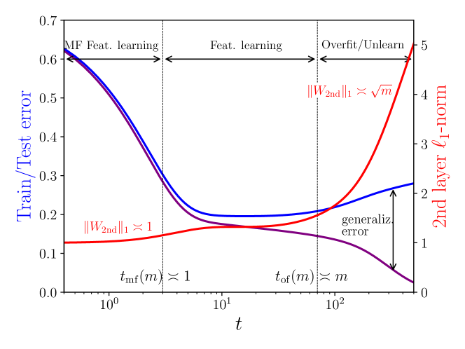
Figure 1: Three dynamical regimes of learning in a two-layer neural networks, with $m$ hidden neurons. Training data comprises $n$ points in $d$ dimensions distributed according to a single index model. We assume $n,m,d$ all large with $n/md=\alpha$ (here $\alpha=0.3$). Blue: test error. Purple: train error. Red: $\ell_{1}$ norm of second-layer weights (a proxy for model complexity).

We address the above general questions within model (1.1), by assuming a simple data distribution. Namely, we assume unstructured feature vectors ${\boldsymbol{x}}_{i}\sim{\sf N}(0,{\boldsymbol{I}}_{d})$, and response variables that depend on a low-dimensional projection of these data:

$$y_{i}=\varphi({\boldsymbol{U}}^{{\sf T}}{\boldsymbol{x}}_{i})+{\varepsilon}_{i}\,,\;\;\;\;{\varepsilon}_{i}\sim{\sf N}(0,\tau^{2})\,,$$ (1.3)

where it is understood that the noise ${\varepsilon}_{i}$ is independent of ${\boldsymbol{x}}_{i}$, ${\boldsymbol{U}}\in{\mathbb{R}}^{d\times k}$ is an orthogonal matrix (${\boldsymbol{U}}^{{\sf T}}{\boldsymbol{U}}={\boldsymbol{I}}_{k}$) and $\varphi:{\mathbb{R}}^{k}\to{\mathbb{R}}$ is a nonlinear function, ${\mathbb{E}}\{\varphi({\boldsymbol{g}})^{2}\}<\infty$ for ${\boldsymbol{g}}$ standard Gaussian. Our main focus will be on the simplest case, namely $k=1$, with $\varphi$ a generic function (in particular ${\mathbb{E}}\{\varphi(G)G\}\neq 0$ for $G\sim{\sf N}(0,1)$).

This data distribution is known as ‘$k$-index model’ and, despite its simplicity, presents a rich variety of phenomena. In particular, when the dimension $d$ becomes large, discovering the latent features ${\boldsymbol{U}}^{{\sf T}}{\boldsymbol{x}}$ is crucial for learning and requires nonlinear processing of the labels $y_{i}$. Indeed, many of the studies mentioned above are preoccupied with studying specific aspects of this model or its variations [BES⁺22, DLS22, AAM22, BEG⁺22].

A visual summary of our results is presented in Figure 1. From a technical viewpoint, we achieve two sets of goals:

1. We use techniques from theoretical physics to derive an approximate asymptotic characterization of the gradient flow dynamics (1.2) in the limit $n,d\to\infty$, with $n/d\to\overline{\alpha}$. This characterization is a ‘dynamical mean field theory’ (DMFT) which is asymptotically exact for a well-defined Gaussian version of the original model.

2. We study this DMFT, with special attention to the large network limit $m\to\infty$ at $\alpha=m\overline{\alpha}$ fixed, for a generic single index model ($k=1$). In this limit, we obtain a separation of time scales in the learning dynamics, with each timescale corresponding to a regime of learning.

Figure 1 illustrates this separation of time scales and emergence of learning regimes (curves are obtained by solving numerically the DMFT equations, see the appendices. This figures refers to learning a single index noisy ($\tau>0$) data distribution with an overparametrized model $\alpha=0.3$. We identify three regimes (below $\boldsymbol{W}_{\mbox{\tiny\rm 2nd}}:={\boldsymbol{a}}/m$ is the vector of second-layer weights in model (1.1)):

$(i)$ Mean field feature learning. $t=O(1)$. The network learns the low-dimensional features ${\boldsymbol{U}}^{{\sf T}}{\boldsymbol{x}}$; the train error and test error decrease while their difference (generalization error) is negligible; the second layer weights remain small $\|\boldsymbol{W}_{\mbox{\tiny\rm 2nd}}\|_{1}=O(1)$.

$(ii)$ Extended feature learning. $1\ll t\ll m$. The train error decreases slowly; the generalization error increases but remains small $\mathscrsfs{R}({\boldsymbol{\theta}}(t))-\widehat{\mathscrsfs{R}}_{n}({\boldsymbol{\theta}}(t))=o(1)$; the test error can evolve non-monotonically, but remains approximately constant. Second-layer weights become large $1\ll\|\boldsymbol{W}_{\mbox{\tiny\rm 2nd}}\|_{1}\ll\sqrt{m}$.

$(iii)$ Overfitting and feature unlearning. $t\gtrsim m$. Train error and test error diverge significantly, i.e. $\mathscrsfs{R}({\boldsymbol{\theta}}(t))-\widehat{\mathscrsfs{R}}_{n}({\boldsymbol{\theta}}(t))$ becomes of order one. At the end of this regime, the train error converges to $0$, i.e. the neural network interpolates the noisy data. The test error instead grows, and its limit value is the one of a (data independent) kernel method: in other words, the model unlearns the low-dimensional structure. Finally, the second weights grow to $\|\boldsymbol{W}_{\mbox{\tiny\rm 2nd}}\|_{1}\asymp\sqrt{m}$, which indeed is the scale required for interpolation.

In Section 2 we provide a more complete account of our results, focusing on the insights it provides on the training dynamics. The derivation of the DMFT equations as well as their detailed analysis is deferred to the appendices. In Section 3 we state two simple rigorous results that confirm the picture arising from DMFT, and in Section 4 we draw some conclusions. We point out some of our results apply to $k$-index models for general fixed $k$. However, a complete analysis of the generic $k\geq 2$ case would require to consider time $t$ diverging logarithmically in $d$, and hence a more complex asymptotics. We expect qualitative results to carry through, but defer this analysis to future work.

2 Main results

We begin by describing the nature of our DMFT approximation in Section 2.1. In Section 2.2, we use this approximation to study the simplest possible setting: pure noise data. Already this case presents a rich phenomenology, and provides useful background. Finally we consider the single-index model in Section 2.3.

As mentioned, we study the high dimensional limit $n,d\to\infty$, with $n/d\to\overline{\alpha}\in(0,\infty)$ (and take the large network limit afterwards.) Throughout, we index sequences by $n$, and it is understood that $d=d_{n}$ satisfies the limit.

2.1 Technique

Notice that each fitting error $F_{i}({\boldsymbol{\theta}})=y_{i}-f({\boldsymbol{x}}_{i};{\boldsymbol{\theta}})$, $i\in\{1,\dots,n\}$ is a random function of the model parameters ${\boldsymbol{\theta}}$. The randomness is due to the randomness in ${\boldsymbol{x}}_{i}$ and in the noise ${\varepsilon}_{i}$. The empirical risk in Eq. (1.2) can be rewritten as

$$\widehat{\mathscrsfs{R}}_{n}({\boldsymbol{\theta}})=\frac{1}{2n}\|{\boldsymbol{F}}({\boldsymbol{\theta}})\|^{2}\,,\;\;\;\;{\boldsymbol{F}}({\boldsymbol{\theta}})=\big{(}F_{1}({\boldsymbol{\theta}}),\dots,F_{n}({\boldsymbol{\theta}})\big{)}\,.$$ (2.1)

Our key approximation consists in replacing the i.i.d. random functions $(F_{i})_{i\leq n}$ by i.i.d. Gaussian processes $(F^{g}_{i})_{i\leq n}$ with matching mean and covariance. While DMFT equations have been recently proven without recurring to this approximation (see [CCM21] and appendices), their structure is simpler in the Gaussian case, which allows us to carry out the large-$m$ analysis.

Computing the covariance of ${\boldsymbol{F}}(\,\cdot\,)$ is a straightforward exercise. We assume for simplicity that an intercept is subtracted so that ${\mathbb{E}}[\sigma(G)]=0$, ${\mathbb{E}}[\varphi({\boldsymbol{G}})]=0$ and otherwise these functions are generic ($G$, $G_{1}$, ${\boldsymbol{G}}$ and so on will denote standard Gaussian vectors). We then have

$${\mathbb{E}}\big{\{}f({\boldsymbol{x}};{\boldsymbol{\theta}}_{1})f({\boldsymbol{x}};{\boldsymbol{\theta}}_{2})\big{\}}=\frac{1}{m^{2}}\langle{\boldsymbol{a}}_{1},h(\boldsymbol{W}_{1}^{{\sf T}}\boldsymbol{W}_{2}){\boldsymbol{a}}_{2}\rangle\,,$$ (2.2)

$${\mathbb{E}}\big{\{}f({\boldsymbol{x}};{\boldsymbol{\theta}})y\big{\}}=\frac{1}{m^{2}}\langle{\boldsymbol{a}},\widehat{\varphi}(\boldsymbol{W}^{{\sf T}}{\boldsymbol{U}})\rangle\,.$$ (2.3)

Recall that ${\boldsymbol{\theta}}=({\boldsymbol{a}},\boldsymbol{W})$ where ${\boldsymbol{a}}\in{\mathbb{R}}^{m}$, $\boldsymbol{W}=({\boldsymbol{w}}_{1},\dots,{\boldsymbol{w}}_{m})\in{\mathbb{R}}^{d\times m}$ are the first layer weights Finally, $h:{\mathbb{R}}\to{\mathbb{R}}$, $\widehat{\varphi}:{\mathbb{R}}^{k}\to{\mathbb{R}}$ encode the activations $\sigma$ and the target function $\varphi$, with $h$ applied entrywise to the matrix $\boldsymbol{W}_{1}^{{\sf T}}\boldsymbol{W}_{2}$.

The covariance of $F_{i}({\boldsymbol{\theta}})=y_{i}-f_{i}({\boldsymbol{x}};{\boldsymbol{\theta}})$ is easily computed from the above, and this defines completely the corresponding Gaussian process $(F^{g}_{i})_{i\leq n}$. We denote the associated risk function $\widehat{\mathscrsfs{R}}^{g}_{n}({\boldsymbol{\theta}}):=\|{\boldsymbol{F}}^{{\boldsymbol{g}}}({\boldsymbol{\theta}})\|^{2}/2n$.

Let us emphasize that the cost function $\widehat{\mathscrsfs{R}}^{g}_{n}({\boldsymbol{\theta}})$ remains highly non-trivial despite the fact that the functions $F_{i}$ are replaced by Gaussian processes. Near-minima of high-dimensional Gaussian processes have a very rich structure, which is a central theme in spin glass theory [MPV87, Tal10]. Additional layers of complexity arise here for two reasons. First, $\widehat{\mathscrsfs{R}}^{g}_{n}({\boldsymbol{\theta}})$ is a sum of squares of Gaussians and, second, the underlying Gaussian process has a significantly more intricate covariance than in standard spin glasses (where typically depends only on the inner product $\langle{\boldsymbol{\theta}}_{1},{\boldsymbol{\theta}}_{2}\rangle$). Recent work explored the simpler case in which $F^{g}_{i}(\,\cdot\,)$ is a Gaussian process with covariance ${\mathbb{E}}\{F^{g}_{i}({\boldsymbol{\theta}}_{1})F^{g}_{i}({\boldsymbol{\theta}}_{2})\}=\xi(\langle{\boldsymbol{\theta}}_{1},{\boldsymbol{\theta}}_{2}\rangle)$ depending uniquely on the inner product [Fyo19, FT22, Urb23, Sub23, MS23, MS24, KD24]. Gradient descent dynamics on these models has been recently studied via DMFT in [KU23a, KU23b]: our work builds on these advances. DMFT was leveraged before to address other questions in high-dimensional statistics and ML [MKUZ19, BP22]. We refer to [BADG06, CCM21] for mathematical results on the DMFT approach.

While $\widehat{\mathscrsfs{R}}^{g}_{n}({\boldsymbol{\theta}})$ has a non-trivial structure, methods from statistical physics can be brought to bear to derive an asymptotic characterization. Namely, define the functions

$$C_{ij}^{n}(t_{1},t_{2})=\langle{\boldsymbol{w}}_{i}(t_{1}),{\boldsymbol{w}}_{j}(t_{2})\rangle\,,\;\;\;\;{\boldsymbol{v}}^{n}_{i}(t):={\boldsymbol{U}}^{{\sf T}}{\boldsymbol{\theta}}_{i}(t)\,,\;\;\;a^{n}_{i}(t)\,.$$ (2.4)

These functions are random (because of the random initialization and the randomness in ${\boldsymbol{F}}^{{\boldsymbol{g}}}$) and depend on $n,d$. However, as $n,d\to\infty$ with $n/d\to\overline{\alpha}$, they converge to non-random limits $(C_{ij}(t_{1},t_{2}))_{i<j\leq m}$, $({\boldsymbol{v}}_{i}(t))_{i\leq m}$, $(a_{i}(t))_{i<j\leq m}$ that are the unique solution of a set of coupled integro-differential equations, see the appendices. We refer to these as to the DMFT equations.

Our main focus is on the behavior of the solutions of these equations for large $m$ and, at first sight, the complexity of the DMFT increases with $m$. An important simplification arises when choosing a symmetric initial condition $a_{i}(0)=a_{0}$ for all $i\leq m$, and $({\boldsymbol{w}}_{i}(0))_{i\leq m}\sim_{iid}{\sf Unif}({\mathbb{S}}^{d-1})$. Namely, the solution of the DMFT equations is symmetric under permutations of the neurons: $C_{ii}(t_{1},t_{2})=C_{d}(t_{1},t_{2})$ for $i\leq m$ and $C_{ij}(t_{1},t_{2})=C_{o}(t_{1},t_{2})$ for $i\neq j\leq m$, while ${\boldsymbol{u}}_{i}(t)={\boldsymbol{u}}(t)$, $a_{i}(t)=a(t)$ for $i\leq m$. We then have a reduction to a set of integro-differential equations on $k+3$ functions, that depend parametrically on $m$.

We use two approaches to study these equations (see appendix):

• Numerical integration for increasing values of $m$ under different initial conditions.

• Asymptotics as $m\to\infty$ (at fixed $\alpha=\overline{\alpha}/m$) via singular perturbation theory [Ber01, Hol13].

For $(b)$, a specific dynamical regime is identified by a scaling of the time variable, which in our case will take the form $t=t_{\#}(m)\cdot\hat{t}$ for a certain fixed function $t_{\#}(m)$ and $\hat{t}=O(1)$ a scaled time. The asymptotics of DMFT quantities in that regime takes the form

$$\lim_{m\to\infty}{\boldsymbol{v}}\Big{(}t_{\#}(m)\cdot\hat{t};m,\overline{\alpha}=\frac{\alpha}{m}\Big{)}={\boldsymbol{v}}_{*}(\hat{t};\alpha)\,.$$ (2.5)

2.2 Training on pure noise

We begin by the case in which the data is pure noise: $y_{i}={\varepsilon}_{i}\sim{\sf N}(0,\tau^{2})$. A by-now-classic experiment [ZBH⁺21] showed that deep learning models have sufficient capacity to achieve vanishing training error even when actual labels are replaced by random ones: they ‘interpolate pure noise.’

The ability of a model ${\mathcal{F}}_{\Theta}=(f(\,\cdot\,;{\boldsymbol{\theta}}):{\boldsymbol{\theta}}\in\Theta)$ to interpolate pure noise is intimately connected to its Gaussian complexity ${\mathcal{G}}({\mathcal{F}}_{\Theta};n):={\mathbb{E}}\sup_{{\boldsymbol{\theta}}\in\Theta}\langle{\boldsymbol{g}},f(\boldsymbol{X};{\boldsymbol{\theta}})\rangle/n$ [Ver18] (Rademacher complexity for binary labels). Indeed, interpolation is impossible unless ${\mathcal{G}}({\mathcal{F}}_{\Theta};n)\geq\tau$. Viceversa, ${\mathcal{G}}({\mathcal{F}}_{\Theta};n)\ll\tau$ ensures good generalization.

An important theorem of Bartlett [Bar96] shows that, for the network (1.1), with a bound on the $\ell_{1}$ norm of second-layer weights, ${\mathcal{G}}({\mathcal{F}}_{\Theta};n)\leq L_{\sigma}\|{\boldsymbol{a}}/m\|_{1}\sqrt{d/n}$ (with $L_{\sigma}$ depending uniquely on the activation function). This means that, in order to interpolate noise, the average magnitude of second layer weights must be $\|{\boldsymbol{a}}\|_{1}/m\geq C_{\sigma,\alpha}\tau\sqrt{m}$ (where $C_{\sigma,\alpha}=\sqrt{\alpha}/L_{\sigma}$ and we recall that $\alpha=(n/md)=\Theta(1)$ is the overparametrization ratio).

Does gradient flow converge to interpolators? Does the neural network produced by gradient flow have vanishing train error (and hence $\|{\boldsymbol{a}}\|_{1}\gtrsim\sqrt{m}$), and yet generalize well?

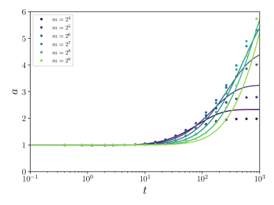
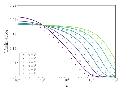
Figure 2: Evolution of second-layer weights (left) and train error (right) when fitting white noise variance with standard deviation $\tau=0.6$. Here we use mean field initialization and $h(z)=(9/10)z+(1/6)z^{3}$. Symbols: SGD results on actual 2-layer networks. Continuous viridis lines: Numerical solution of the DMFT equations.

We will study the dynamics of training on pure noise under three different setings for the evolution of second layer weights: $a(0)\asymp\sqrt{m}$ not evolving with gradient flow; $a(0)\asymp\sqrt{m}$ evolving; $a(0)\asymp 1$ evolving. The first setting is the simpler to study, but we will show that the long-time behavior of the other two is closely related to the first one via an adiabatic approximation.

As an introduction, Figure 2 compares the DMFT predictions to simulations using SGD to train an actual two layer networks. In this figure we initialize $a(0)=1$, and $a(t)$ evolving. We observe that the theory describes well —both qualitatively and quantitatively— the empirical results, despite the Gaussian approximation in our DMFT and the difference between SGD and gradient flow. We also observe that second-layer weights remain roughly equal until a large time $t_{\#}(m)$, which appears to increase with $m$. Roughly at the same time, train error starts to decrease rapidly and converges to zero. Our analysis will make precise this qualitative description.

We also note that, for $\varphi=0$, the problem depends on ${\boldsymbol{a}}$, $\tau$ only through the ratio ${\boldsymbol{a}}/\tau$. Unless stated otherwise, we can think that $\tau=1$ is fixed.

2.2.1 Fixed $a$, lazy initialization

We set $a(t)=\gamma\sqrt{m}$ with $\gamma$ independent of $m$ which does not change with time. Note that ${\mathcal{G}}({\mathcal{F}}_{\Theta};n)\asymp\gamma/\sqrt{\alpha}$ and hence such a network can interpolate pure noise if $\gamma$ is larger than a suitable constant (depending on $\alpha$). Indeed, DMFT predicts a sharp phase transition. For $\alpha\in(0,1)$, GF converges to vanishing train error with high probability if $\gamma>\gamma_{\mbox{\tiny\rm GF}}(\alpha,m)$, and converges to a strictly positive training error if $\gamma<\gamma_{\mbox{\tiny\rm GF}}(\alpha,m)$. The threshold $\gamma_{\mbox{\tiny\rm GF}}(\alpha,m)$ converges to a limit $\gamma_{\mbox{\tiny\rm GF}}^{*}(\alpha)\in(0,1)$ as $m\to\infty$. Informally $\gamma_{\mbox{\tiny\rm GF}}^{*}(\alpha)$ is the minimum complexity $\gamma$ for a very large network to interpolate noise.

In other words, for $\gamma<\gamma_{\mbox{\tiny\rm GF}}^{*}(\alpha)$, we have $\lim_{n,d\to\infty}\widehat{\mathscrsfs{R}}_{n}^{g}({\boldsymbol{\theta}}(t))={e}_{\mbox{{\rm\footnotesize tr}}}(t;m,\gamma_{0})$, and

$$\lim_{t\to\infty}\lim_{m\to\infty}{e}_{\mbox{{\rm\footnotesize tr}}}(t;m,\gamma_{0})=\begin{cases}e_{*}(\gamma_{0})>0&\mbox{ for $\gamma_{0}<\gamma_{\mbox{\tiny\rm GF}}^{*}(\alpha)$,}\\ 0&\mbox{ for $\gamma_{0}\geq\gamma_{\mbox{\tiny\rm GF}}^{*}(\alpha)$.}\end{cases}$$ (2.6)

The function $e_{*}(\gamma)$ will play an important role below.

2.2.2 Dynamical $a$, lazy initialization

We use the initialization $a(0)=\gamma_{0}\sqrt{m}$ with $\gamma_{0}$ independent of $m$, and let $a(t)$ evolve according to gradient flow (1.2); $\gamma(t)=a(t)/\sqrt{m}$ evolves accordingly. DMFT predicts that, if $\gamma_{0}$ is a small constant ($\gamma_{0}<\gamma_{\mbox{\tiny\rm GF}}^{*}(\alpha)$), then $\gamma(t)$ grows in time until it becomes large enough for interpolation to take place.

More precisely, for large $m$, we identify three dynamical regimes.

First dynamical regime: $t=O(1/m)$. $\gamma(t)=\gamma_{0}+o_{m}(1)$: second layer weights remain approximately constant. The train error decreases because of the evolution of first layer weights which change $\|{\boldsymbol{w}}_{i}(t)-{\boldsymbol{w}}_{i}(0)\|=O(1/\sqrt{m})$. At the end of this regime, the network approximates the zero function $f(\,\cdot\,;{\boldsymbol{\theta}})\approx 0$.

Second dynamical regime: $t=\Theta(1)$. Also in this regime $\gamma(t)=\gamma_{0}+o_{m}(1)$ and hence the model complexity remains unchanged. However, first-layer weights change significantly: $\|{\boldsymbol{w}}_{i}(t)-{\boldsymbol{w}}_{i}(0)\|=\Theta(1)$. The train error decreases appreciably in this phase and has a well defined limit $\lim_{m\to\infty}\widehat{\mathscrsfs{R}}^{g}_{n}({\boldsymbol{\theta}}(t))={e}^{\mbox{\tiny\rm lz2}}_{\mbox{{\rm\footnotesize tr}}}(t;\gamma_{0})$, with $t\mapsto{e}^{\mbox{\tiny\rm lz2}}_{\mbox{{\rm\footnotesize tr}}}(t;\gamma_{0})$ a monotone decreasing function.

The long-time behavior of ${e}^{\mbox{\tiny\rm lz2}}_{\mbox{{\rm\footnotesize tr}}}(t;\gamma_{0})$ depends on the complexity at initialization $\gamma_{0}$. If $\gamma_{0}>\gamma_{\mbox{\tiny\rm GF}}(\alpha)$, then $\lim_{t\to\infty}{e}^{\mbox{\tiny\rm lz2}}_{\mbox{{\rm\footnotesize tr}}}(t;\gamma_{0})=0$ and interpolation takes place within this dynamical regime. If $\gamma_{0}<\gamma_{\mbox{\tiny\rm GF}}(\alpha)$, then $\lim_{t\to\infty}{e}^{\mbox{\tiny\rm lz2}}_{\mbox{{\rm\footnotesize tr}}}(t;\gamma_{0})=e_{*}(\gamma_{0})>0$. This coincides with the asymptotic train error at fixed $\gamma$, cf. Sec. 2.2.1. In the latter case, a third dynamical regime emerges and leads to interpolation on significantly longer time scales.

Third dynamical regime: $t=\Theta(m)$. $\gamma(t)$ increases significantly: $\gamma(t)-\gamma_{0}=\Theta(1)$. At the same time, the train error decreases on the same time scale, reaching $0$ when $\gamma(t)\approx\gamma^{*}_{\mbox{\tiny\rm GF}}(\alpha)$. The model complexity $\gamma(t)$ and training error $\widehat{\mathscrsfs{R}}^{g}_{n}({\boldsymbol{\theta}}(t))$ obey a scaling law. Namely, for any fixed $z\in(0,\infty)$, as $m\to\infty$, we have

$$a(mz)={\gamma}^{\mbox{\tiny\rm lz3}}(z;\gamma_{0})\sqrt{m}+o_{m}(\sqrt{m})\,,\;\;\;\;\;\;\;\;\;\widehat{\mathscrsfs{R}}^{g}_{n}({\boldsymbol{\theta}}(mz))={e}^{\mbox{\tiny\rm lz3}}_{\mbox{{\rm\footnotesize tr}}}(z;\gamma_{0})+o_{m}(1)\,.$$ (2.7)

Informally, the scaling law implies that, in this time scale, $a(t)\approx\sqrt{m}{\gamma}^{\mbox{\tiny\rm lz3}}(t/m;\gamma_{0})$ and $\widehat{\mathscrsfs{R}}^{g}_{n}({\boldsymbol{\theta}}(t))\approx{e}^{\mbox{\tiny\rm lz3}}_{\mbox{{\rm\footnotesize tr}}}(t/m;\gamma_{0})$. We have $\lim_{z\to 0}{\gamma}^{\mbox{\tiny\rm lz3}}(z;\gamma_{0})=\gamma_{0}$ hence matching the previous two regimes.

As further discussed below, the DMFT solution points at a separation of dynamical degrees of freedom, with the complexity $\gamma(t)$ acting as a slow variable, while the others variables evolving rapidly [VK85, PS08].

2.2.3 Dynamical $a$, mean field initialization

We now choose an initialization $a(0)=a_{0}$ that is independent of $m$, and let $a(t)$ evolve with gradient flow. Figure 3 compares numerical experiments with SGD on actual two-layer networks and numerical integration of the DMFT equations.

At initialization, the Gaussian complexity of the models with the given $\|{\boldsymbol{a}}\|_{1}$ is ${\mathcal{G}}({\mathcal{F}}_{\Theta};n)\lesssim\sqrt{d/n}=1/\sqrt{m\alpha}$. In order to achieve interpolation, $a(t)$ has to grow and become of order $\sqrt{m}$. For large $m$, DMFT predicts that the growth of $a(t)$ (and hence model complexity) takes place in three distinct dynamical regimes, each corresponding to a different time scale, as described below.

First dynamical regime: $t=O(1)$. Second layer weights do not move $a(t)=a_{0}+o_{m}(1)$, while first layer weights change by a small amount $\|{\boldsymbol{w}}_{i}(0)-{\boldsymbol{w}}_{i}(t)\|=o_{m}(1)$ to achieve approximately $0$ mean: $\sum_{i\leq m}{\boldsymbol{w}}_{i}\approx\boldsymbol{0}$. The model learned at the end of this regime is a good approximation of the null model $f({\boldsymbol{x}};{\boldsymbol{\theta}})\approx 0$. Correspondingly, $\widehat{\mathscrsfs{R}}_{n}({\boldsymbol{\theta}}(t))=\widehat{\mathscrsfs{R}}_{n,\mbox{\tiny\rm null}}+o_{m}(1)$ with $\widehat{\mathscrsfs{R}}_{n,\mbox{\tiny\rm null}}:=\tau^{2}/2$ the error of the null model.

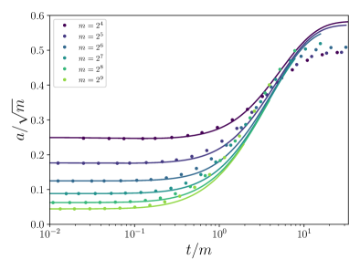
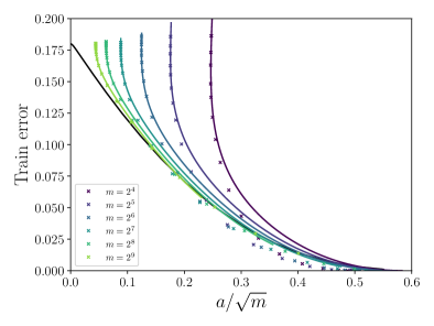
Figure 3: Evolution of second-layer weights (left) and train error vs second-layer weights (right), under mean field initialization. Same setting as in Fig. 2, except we scale $t$ and $a$ according to the interpolation scaling law of Eq. (2.7). Symbols: SGD results. Continuous viridis lines: DMFT. Continuous black line: scaling law (computed with fixed second layer weights).

Second dynamical regime: $t=\Theta(\sqrt{m})$. On this time scale, second layer begin to evolve according to $a(t)={a}^{\mbox{\tiny\rm mf2}}(t/\sqrt{m})+o_{m}(1)$, while first layer weights change significantly $\|{\boldsymbol{w}}_{i}(t)-{\boldsymbol{w}}_{i}(0)\|=\Theta(1)$. While the dynamics on this regime is highly non-trivial, the change is not large enough to change the train error $\widehat{\mathscrsfs{R}}_{n}({\boldsymbol{\theta}}(t))$ appreciably. We still have $\widehat{\mathscrsfs{R}}_{n}({\boldsymbol{\theta}}(t))\approx\widehat{\mathscrsfs{R}}_{n,\mbox{\tiny\rm null}}+o_{m}(1)$. Equations for the scaling function ${a}^{\mbox{\tiny\rm mf2}}(\,\cdot\,)$ are given in the appendices. It turns out that, in this regime, the dynamics of the $m$ neurons is asymptotically equivalent to the dynamics of $m$ systems coupled uniquely via $a(t)$. Further, each of the neurons follows a dynamics that is equivalent to the dynamics of a ‘reduced model.’ In the Gaussian process setting, the reduced model is the celebrated mixed spherical spin glass model [CK93, FFRT20].

Third dynamical regime: $t=\Theta(m)$. On this scale, second layer weights finally grow to be of order $\sqrt{m}$ and interpolation becomes possible. Namely, for any fixed $z$, as $m\to\infty$, we have

$$a(mz)=\sqrt{m}{\gamma}^{\mbox{\tiny\rm mf3}}(z)+o_{m}(\sqrt{m})\,,\;\;\;\;\;\widehat{\mathscrsfs{R}}_{n}({\boldsymbol{\theta}}(mz))={e}^{\mbox{\tiny\rm mf3}}_{\mbox{{\rm\footnotesize tr}}}(z)+o_{m}(1)\,.$$ (2.8)

The functions ${\gamma}^{\mbox{\tiny\rm mf3}}$, ${e}^{\mbox{\tiny\rm mf3}}_{\mbox{{\rm\footnotesize tr}}}$ are close (and potentially identical to) the $\gamma_{0}\to 0$ limit of the functions ${\gamma}^{\mbox{\tiny\rm lz3}}$, ${e}^{\mbox{\tiny\rm lz3}}_{\mbox{{\rm\footnotesize tr}}}$ of Eq. (2.7). We have ${\gamma}^{\mbox{\tiny\rm mf3}}(z)=\gamma_{1}z+o(z)$ as $z\to 0$ which suggests to $a(t)\asymp t/\sqrt{m}$ for $\sqrt{m}\ll t\ll m$, thus matching the previous time scale. At the other extreme, ${\gamma}^{\mbox{\tiny\rm mf3}}(z)\to\overline{\gamma}^{*}_{\mbox{\tiny\rm GF}}(\alpha)\approx\gamma^{*}_{\mbox{\tiny\rm GF}}(\alpha)$ as $z\to\infty$, i.e. weights grow until $a(t)\approx\gamma^{*}_{\mbox{\tiny\rm GF}}(\alpha)\sqrt{m}$ and at that point interpolation takes place.

This third dynamical regime is illustrated in Fig. 3 which compares numerical simulations with SGD and DMFT in terms of the rescaled variables $t/m$, $a(t)/\sqrt{m}$ and $\widehat{\mathscrsfs{R}}_{n}({\boldsymbol{\theta}}(t))$. In the left plot, we plot $a(t)/\sqrt{m}$ versus $t/m$ for several values of $m$. We obtain approximate collapse of data obtained for different values of $m$, confirming the the ansatz in the third dynamical regime.

Remark 2.1.

While our analytical derivations are based on the Gaussian approximation $\widehat{\mathscrsfs{R}}^{g}_{n}({\boldsymbol{\theta}})$ to the empirical risk function, we expect our qualitative conclusions to apply to the original empirical risk $\widehat{\mathscrsfs{R}}_{n}({\boldsymbol{\theta}})$. In particular, we expect the same time-scale separation to arise in this context. This is partially confirmed by our numerical simulations, and by the rigorous results of Section 3.

2.2.4 Adiabatic evolution

Consider again the third dynamical regime under lazy initialization. In Fig. 3 right frame, we plot $e_{\mbox{{\rm\footnotesize tr}}}(t)$ parametrically against $a(t)/\sqrt{m}$ for several values of $m$. As $m$ increase, the curves appear to converge to a well-defined limit. To characterize this limit, recall the ansatz (2.8) and the fact that function ${\gamma}^{\mbox{\tiny\rm mf3}}$ describing the increase in complexity is monotone, mapping $(0,\infty)$ to $(0,\overline{\gamma}^{*}_{\mbox{\tiny\rm GF}}(\alpha))$ (with $\overline{\gamma}^{*}_{\mbox{\tiny\rm GF}}(\alpha))\approx\gamma^{*}_{\mbox{\tiny\rm GF}}(\alpha)$). We can therefore define the inverse function $\gamma\mapsto({\gamma}^{\mbox{\tiny\rm mf3}})^{-1}(\gamma)$ and

$${{\varepsilon}}^{\mbox{\tiny\rm mf}}(\gamma):={e}^{\mbox{\tiny\rm mf3}}_{\mbox{{\rm\footnotesize tr}}}(({\gamma}^{\mbox{\tiny\rm mf3}})^{-1}(\gamma))\,.$$ (2.9)

Under the ansatz (2.8), the finite-$m$ curves of Fig. 3 converge to the limit $(\gamma,{{\varepsilon}}^{\mbox{\tiny\rm mf}}(\gamma))$.

Note that we could have defined an analogous curve for the lazy initialization. Namely, for $\gamma\in(\gamma_{0},\gamma^{*}_{\mbox{\tiny\rm GF}}(\alpha))$ ${{\varepsilon}}^{\mbox{\tiny\rm lz}}(\gamma):={e}^{\mbox{\tiny\rm lz3}}_{\mbox{{\rm\footnotesize tr}}}(({\gamma}^{\mbox{\tiny\rm lz3}})^{-1}(\gamma;\gamma_{0});\gamma_{0})$ (where the inverse function is defined by ${\gamma}^{\mbox{\tiny\rm lz3}}(({\gamma}^{\mbox{\tiny\rm lz3}})^{-1}(\gamma;\gamma_{0});\gamma_{0})=\gamma$). Our analysis of the DMFT equations implies that ${{\varepsilon}}^{\mbox{\tiny\rm lz}}(\gamma)\approx{{\varepsilon}}^{\mbox{\tiny\rm mf}}(\gamma)$.

In Fig. 3, we also plot the curve $e_{*}(\gamma)$ defined in Sec. 2.2.1 which gives the asymptotic training error when keeping second-layer weights fixed (as computed from numerically solving the DMFT equations). The finite-$m$ curves appear to converge to the latter, i.e.:

$${{\varepsilon}}^{\mbox{\tiny\rm mf}}(\gamma)\approx{{\varepsilon}}^{\mbox{\tiny\rm lz}}(\gamma)\approx e_{*}(\gamma)\,.$$ (2.10)

This identity has a simple interpretation. For large $m$, we have a fast-slow separation of degrees of freedom (a classical phenomenon in multiscale analysis [PS08]). The model complexity $\gamma(t)$ grows slowly, while all other quantities in the DMFT equations relax rapidly. At any given $t$, the dynamics of the other degrees of freedom is nearly the same as if the complexity was kept fixed at $\gamma(t)$ (as in Sec. 2.2.1).

While our numerical integration of the DMFT equations is consistent with the hypothesis that (2.10) is an exact equality, establishing whether exact equality holds is an open problem.

2.3 Training on data with latent structure

We next consider training on data from a single-index model. While we expect the time-scale separation discussed hear to hold for general $k$-index models, some subtleties arise with the high-dimensional asymptotics studied here. We discuss the generalization to $k\geq 2$ in Section 4. As before, we separately analyze two types of initializations: lazy and mean field.

Figure 4: Train/test error (right) when fitting data from a single index model, with $h(z)=\widehat{\varphi}(z)=(9/10)z+z^{2}/2$, $\tau=0.3$ and $\alpha=0.3$. Lines correspond to predictions from the DMFT (continuous: train error; dashed: test error). The inset on the right reports the value of the test error at the plateau, as a function of $m$ (green line is the $m\to\infty$ value). Right: Same data plotted versus $t$.

2.3.1 Lazy initialization

We initialize $a(0)=\gamma_{0}\sqrt{m}$, and let $\gamma(t)$ evolve according to gradient flow alongside first-layer weights. DMFT predicts the emergence of three dynamical regimes for large $m$, in analogy to the case of pure noise data. For an illustration, we refer to Fig. 4.

First dynamical regime: $t=O(1/m)$. Second layer weights do not change significantly $\gamma(t)=\gamma_{0}+o_{m}(1)$, while first layer-weights move by $\|{\boldsymbol{w}}_{i}(t)-{\boldsymbol{w}}_{i}(0)\|=\Theta(1/\sqrt{m})$. Because the weights $a_{i}(t)$ are of order $\sqrt{m}$, even an $O(1/\sqrt{m})$ change in the ${\boldsymbol{w}}_{i}$ leads to a significant decrease in test error and train error.

Train and test error are close to each other. Namely, the following limits are well defined

$$\lim_{n,d\to\infty}\widehat{\mathscrsfs{R}}_{n}({\boldsymbol{\theta}}(t))=e_{\mbox{{\rm\footnotesize tr}}}(t;\varphi,\gamma_{0},m,\alpha)\,,\;\;\;\;\;\lim_{n,d\to\infty}\mathscrsfs{R}({\boldsymbol{\theta}}(t))=e_{\mbox{\rm\footnotesize ts}}(t;\varphi,\gamma_{0},m,\alpha)\,.$$ (2.11)

with $\lim_{m\to\infty}e_{\mbox{{\rm\footnotesize tr}}}(\hat{t}/m;\varphi,\gamma_{0},m,\alpha)=\lim_{m\to\infty}e_{\mbox{\rm\footnotesize ts}}(\hat{t}/m;\varphi,\gamma_{0},m,\alpha)=:{e}^{\mbox{\tiny\rm lz1}}(\hat{t};\varphi,\gamma_{0},\alpha)$.

For large scaled time $\hat{t}$, the error ${e}^{\mbox{\tiny\rm lz1}}(\hat{t};\varphi,\gamma_{0},\alpha)$ converges to the error of the best linear approximation to $f_{*}$. This dynamical regime follows the qualitative predictions of NTK theory, and is essentially linear in the weights ${\boldsymbol{w}}_{i}$.

Second dynamical regime: $t=\Theta(1)$. This regime is completely analogous to the second dynamical regime with pure noise data and lazy initialization, cf. Section 2.2.2. Second layer weights do not change significantly: $\gamma(t)=\gamma_{0}+o_{m}(1)$, while first layer weights change significantly $\|{\boldsymbol{w}}_{i}(t)-{\boldsymbol{w}}_{i}(0)\|=\Theta(1)$. However they change orthogonally to the latent subspace ${\boldsymbol{U}}$ and hence the test error does not change: no actual learning takes place in this regime.

More formally, train and test error have well defined limits

$${e}^{\mbox{\tiny\rm lz2}}_{\mbox{{\rm\footnotesize tr}}}(t;\varphi,\gamma_{0},\alpha):=\lim_{m\to\infty}e_{\mbox{{\rm\footnotesize tr}}}(t;\varphi,\gamma_{0},m,\alpha)\,,\;\;\;{e}^{\mbox{\tiny\rm lz2}}_{\mbox{\rm\footnotesize ts}}(t;\varphi,\gamma_{0},\alpha):=\lim_{m\to\infty}e_{\mbox{\rm\footnotesize ts}}(t;\varphi,\gamma_{0},m,\alpha)\,.$$ (2.12)

However, ${e}^{\mbox{\tiny\rm lz2}}_{\mbox{\rm\footnotesize ts}}(t;\varphi,\gamma_{0},\alpha)$ is constant

$${e}^{\mbox{\tiny\rm lz2}}_{\mbox{\rm\footnotesize ts}}(t;\varphi,\gamma_{0},\alpha)=\lim_{\hat{t}\to\infty}{e}^{\mbox{\tiny\rm lz1}}(\hat{t};\varphi,\gamma_{0},\alpha)=\frac{1}{2}\left(\tau^{2}+\|\varphi\|^{2}-\frac{\|\nabla\widehat{\varphi}({\mathbf{0}})\|^{2}}{h^{\prime}(0)}+\gamma_{0}^{2}(h(1)-h^{\prime}(0))\right)\,.$$ (2.13)

Since the ${\boldsymbol{w}}_{i}$’s move orthogonally to the latent space, their dynamics is equivalent (for large $m$) to the one in the pure noise setting, modulo a redefinition of the covariance $h$. The right plot in Fig. 4 illustrates this.

Third dynamical regime: $t=\Theta(m)$. Also this dynamical regime is analogous to the one in the case of pure noise data, cf. Sec. 2.2.2. Its qualitative properties depend whether or not $\gamma_{0}$ is larger than an interpolation threshold $\gamma^{*}_{\mbox{\tiny\rm GF}}(\alpha,\varphi,\tau)$, which generalizes the threshold $\gamma^{*}_{\mbox{\tiny\rm GF}}(\alpha)=\gamma^{*}_{\mbox{\tiny\rm GF}}(\alpha,0,1)$ introduced in Sec. 2.2.2. Because of the equivalence between the two dynamics mentioned above, the following relation exists:

$$\gamma^{*}_{\mbox{\tiny\rm GF}}(\alpha,\varphi,\tau)=\Big{(}\tau^{2}+\|\varphi\|^{2}-\frac{\|\nabla\hat{\varphi}(\boldsymbol{0})\|^{2}}{h^{\prime}(0)}\Big{)}^{1/2}\gamma^{*}_{\mbox{\tiny\rm GF}}(\alpha)\,.$$ (2.14)

For $\gamma_{0}>\gamma^{*}_{\mbox{\tiny\rm GF}}(\alpha,\varphi,\tau)$, interpolation is achieved during the second dynamical regime, no further evolution takes place. For $\gamma_{0}<\gamma^{*}_{\mbox{\tiny\rm GF}}(\alpha,\varphi,\tau)$, we have, for any $z\in(0,\infty)$, as $m\to\infty$,

$$\gamma(mz)={\gamma}^{\mbox{\tiny\rm lz3}}(z)+o_{m}(1),\;\;\;e_{\mbox{{\rm\footnotesize tr}}}(mz)={e}^{\mbox{\tiny\rm lz3}}_{\mbox{{\rm\footnotesize tr}}}(z)+o_{m}(1),\;\;\;e_{\mbox{\rm\footnotesize ts}}(mz)={e}^{\mbox{\tiny\rm lz3}}_{\mbox{\rm\footnotesize ts}}(z)+o_{m}(1)\,,$$ (2.15)

with ${\gamma}^{\mbox{\tiny\rm lz3}}(z)$ growing to $\overline{\gamma}^{*}_{\mbox{\tiny\rm GF}}(\alpha,\varphi,\tau)\approx\gamma^{*}_{\mbox{\tiny\rm GF}}(\alpha,\varphi,\tau)$ and ${e}^{\mbox{\tiny\rm lz3}}_{\mbox{{\rm\footnotesize tr}}}(z)$ decreasing to $0$ as $z\to\infty$. In other words, interpolation is achieved on this third regime. Further ${e}^{\mbox{\tiny\rm lz3}}_{\mbox{\rm\footnotesize ts}}(z)$ increase from $\gamma_{0}$ approximately to the test error predicted in Eq. (2.13), with $\gamma_{0}$ replaced by $\gamma^{*}_{\mbox{\tiny\rm GF}}(\alpha,\varphi,\tau)$.

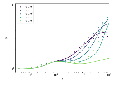
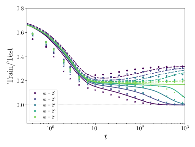
Figure 5: Training dynamics under a single-index model with $h(q)=\widehat{\varphi}(q)=(9/10)q+q^{3}/6$, $\tau=0.3$ and $\alpha=0.3$. Left: second-layer weights. Right: train and test error. Symbols are empirical results for SGD with actual two-layer neural networks with $d=200$, $n=\alpha md$. Lines correspond to predictions from the DMFT (on the right, continuous: train error; dashed: test error).

2.3.2 Mean field initialization

We initialize $a(0)=a_{0}$, independent of $m$ and let second layer weights evolve according to gradient flow. By analyzing the DMFT equations, we observe two dynamical regimes for large $m$. We will refer to them as ‘first’ and ‘third regime’ since they are in correspondence with the first and third dynamical regimes in the pure noise case, see Sec. 2.2.3. For an illustration, we refer to Figs. 5, 6.

First dynamical regime: $t=O(1)$. Both first and second layer weights change by order one: $a(t)=a_{0}+\Theta(1)$ and $\|{\boldsymbol{w}}_{i}(t)-{\boldsymbol{w}}_{i}(0)\|=\Theta(1)$. and as a consequence test and train error decrease significantly. In this regime, the two errors remain close to each other and their evolution is well captured by the mean field theory of [MMN18, CB18], as specialized to the case of spherically invariant distributions [BMZ24, ASKL23].

Namely, $\lim_{t\to\infty}a(t)={a}^{\mbox{\tiny\rm mf1}}(t)$, $\lim_{t\to\infty}{\boldsymbol{v}}(t)={{\boldsymbol{v}}}^{\mbox{\tiny\rm mf1}}(t)$, and DMFT reduces to a system of $k+1$ ordinary differential equations for the $k+1$ scalar variables $({a}^{\mbox{\tiny\rm mf1}}(t),{{\boldsymbol{v}}}^{\mbox{\tiny\rm mf1}}(t))$

$$\begin{split}\partial_{t}{{\boldsymbol{v}}}^{\mbox{\tiny\rm mf1}}(t)&=\alpha{a}^{\mbox{\tiny\rm mf1}}(t){\boldsymbol{Q}}_{{{\boldsymbol{v}}}^{\mbox{\tiny\rm mf1}}(t)}\Big{(}\nabla\hat{\varphi}({{\boldsymbol{v}}}^{\mbox{\tiny\rm mf1}}(t))-{a}^{\mbox{\tiny\rm mf1}}(t)h^{\prime}(\|{{\boldsymbol{v}}}^{\mbox{\tiny\rm mf1}}(t)\|^{2}){{\boldsymbol{v}}}^{\mbox{\tiny\rm mf1}}(t)\Big{)}\,,\\ \partial_{t}{a}^{\mbox{\tiny\rm mf1}}(t)&=\alpha\hat{\varphi}({{\boldsymbol{v}}}^{\mbox{\tiny\rm mf1}}(t))-\alpha{a}^{\mbox{\tiny\rm mf1}}(t)h(\|{{\boldsymbol{v}}}^{\mbox{\tiny\rm mf1}}(t)\|^{2})\,,\end{split}$$ (2.16)

where ${\boldsymbol{Q}}_{{\boldsymbol{v}}}:={\boldsymbol{I}}_{k}-{\boldsymbol{v}}{\boldsymbol{v}}^{{\sf T}}$. As mentioned above, train and test error coincide in the large width limit

$$\lim_{m\to\infty}e_{\mbox{{\rm\footnotesize tr}}}(t)=\lim_{m\to\infty}e_{\mbox{\rm\footnotesize ts}}(t)={e}^{\mbox{\tiny\rm mf1}}(t)\,,$$ (2.17)

$${e}^{\mbox{\tiny\rm mf1}}(t)=\frac{1}{2}\left[\tau^{2}+\|\varphi\|^{2}-2{a}^{\mbox{\tiny\rm mf1}}(t)\hat{\varphi}({{\boldsymbol{v}}}^{\mbox{\tiny\rm mf1}}(t))+{a}^{\mbox{\tiny\rm mf1}}(t)^{2}h(\|{{\boldsymbol{v}}}^{\mbox{\tiny\rm mf1}}(t)\|^{2})\right]\,.$$ (2.18)

In the case $k=1$ and $\widehat{\varphi}(z)=h(z)$, we have that ${a}^{\mbox{\tiny\rm mf1}}=1$, ${v}^{\mbox{\tiny\rm mf1}}=1$ is a fixed point of Eq. (2.16), and indeed the only fixed point with ${v}^{\mbox{\tiny\rm mf1}}>0$. If $h^{\prime}(0)>0$, then, we have $({a}^{\mbox{\tiny\rm mf1}}(t),{v}^{\mbox{\tiny\rm mf1}}(t))\to(1,1)$ as $t\to\infty$, and therefore test and train error converge to the Bayes error ${e}^{\mbox{\tiny\rm mf1}}(t)\to\tau^{2}/2$. This is of course significantly smaller than the test error achieved with lazy initialization, cf. Sec. 2.3.1. The separation between lazy and mean-field initialization is expected because feature learning takes place in the mean field regime.

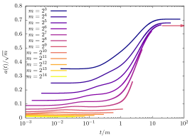
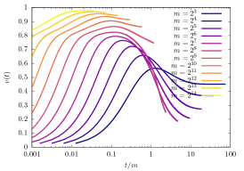
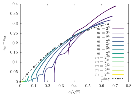
Figure 6: Left Panel: the second layer weights on the scale $\sqrt{m}$ as a function of $t/m$. Curves appear to collapse on a master curve. The rose arrow denotes $\gamma_{GF}^{*}$ and the curves appear to converge to that limit. Central panel: the projection of the first layer weights on the latent space in the single index model as a function of time on timescales of order $m$. Right panel: the difference between test and train error as a function of the second layer weights on the scale $\sqrt{m}$. The finite $m$ curve are approaching a scaling curve which coincides with the one obtained by evaluating the same quantity but with a lazy initialization and fixed second layer weights.

Instability of the first dynamical regime. It is possible to compute $O(1/m)$ corrections to the mean field asymptotics described above (see Appendix). We obtain, in particular:

$$a(t)={a}^{\mbox{\tiny\rm mf1}}(t)+\frac{1}{m}\tilde{a}(t)+o(1/m)\,,\;\;\;\lim_{t\to\infty}\frac{\tilde{a}(t)}{t}=a_{*}\in(0,\infty)\,.$$ (2.19)

If we assume this result holds beyond $t=O(1)$, then we obtain $a(t)\approx{a}^{\mbox{\tiny\rm mf1}}(t)+a_{*}t/m$ for $t\gg 1$, which suggests that the mean field asymptotics breaks down for $t=\Theta(m)$.

Third dynamical regime: $t=\Omega(m)$. For $t\gtrsim m$, we observe that the second layer weights grow to achieve $a(t)\asymp\sqrt{m}$, the projection onto the latent space decreases to ${\boldsymbol{v}}(t)\asymp 1/\sqrt{m}$, and train and test error diverge, eventually achieving $e_{\mbox{{\rm\footnotesize tr}}}(t)\approx 0$ and test error significantly larger than the Bayes error achieved earlier. We refer to this phenomenon as ‘feature unlearning.’

Dynamics on this time scale is illustrated by Fig. 6 that reports solutions of the DMFT equations. We observe the increase of $a(t)$ and decrease of $v(t)$. Further, the increase in generalization error $e_{\mbox{\rm\footnotesize ts}}(t)-e_{\mbox{{\rm\footnotesize tr}}}(t)$ is directly related to $a(t)/\sqrt{m}$ becoming of order $1$.

Denoting by $t_{0}(m;c)$ the time at which $a(t)=c\sqrt{m}$ (for $c$ a small constant), we expect the existence of a window size $w(m)$ such that

$$\lim_{m\to\infty}\frac{a\big{(}t_{0}(m;c)+z\,w(m)\big{)}}{\sqrt{m}} ={\gamma}^{\mbox{\tiny\rm mf3}}(z)\,,\;\;\;\;\;\;\lim_{m\to\infty}e_{\mbox{{\rm\footnotesize tr}}/\mbox{\rm\footnotesize ts}}\big{(}t_{0}(m;c)+z\,w(m)\big{)}={e}^{\mbox{\tiny\rm mf3}}_{\mbox{{\rm\footnotesize tr}}/\mbox{\rm\footnotesize ts}}(z)\,,$$ (2.20)

where ${\gamma}^{\mbox{\tiny\rm mf3}}(z)$, ${e}^{\mbox{\tiny\rm mf3}}_{\mbox{{\rm\footnotesize tr}}}(z)$, ${e}^{\mbox{\tiny\rm mf3}}_{\mbox{\rm\footnotesize ts}}(z)$ are scaling functions describing the dynamics on this timescale. We expect $t_{0}(m;c)=t_{*}(c)m+o(m)$, and $w(m)\lesssim t_{0}(m;c)$, but our numerical solutions are not sufficient to determine the precise scaling. On the other hand, it appears that at large times, the complexity converges close the interpolation threshold (see left plot in Fig. 6):

$$\lim_{z\to\infty}{\gamma}^{\mbox{\tiny\rm mf3}}(z)=\overline{\gamma}^{*}_{\mbox{\tiny\rm GF}}(\alpha,\varphi,\tau)\approx\gamma^{*}_{\mbox{\tiny\rm GF}}(\alpha,\varphi,\tau)\,.$$ (2.21)

Finally, the evolution of train and test error for $a(t)\asymp\sqrt{m}$ appears to match the behavior at fixed second-layer weights. Namely, in analogy with Section 2.2.4, we define two functions

$${{\varepsilon}}^{\mbox{\tiny\rm mf}}_{\mbox{{\rm\footnotesize tr}}/\mbox{\rm\footnotesize ts}}(\gamma):=\lim_{m\to\infty}e_{\mbox{{\rm\footnotesize tr}}/\mbox{\rm\footnotesize ts}}(t_{0}(m;\gamma),m)\,.$$ (2.22)

We observe that the limit curves $(\gamma,{{\varepsilon}}^{\mbox{\tiny\rm mf}}_{\mbox{{\rm\footnotesize tr}}}(\gamma))$, $(\gamma,{{\varepsilon}}^{\mbox{\tiny\rm mf}}_{\mbox{\rm\footnotesize ts}}(\gamma))$, match closely asymptotic train and test error obtained by fixing $a(t)=\gamma\sqrt{m}$, and not letting second-layer weight evolve. This confirms the hypothesis that $\gamma(t)$ is a slow variabes, while others converge as if $\gamma$ was fixed.

3 Lower bounding the overfitting timescale

In this section we rigorously establish two results that confirm some elements of the scenario developed via DMFT the previous sections. The first result implies that (under mean field initialization) overfitting cannot take place too early.

Lemma 3.1.

Under the GF dynamics (1.2), and the data distribution in the introduction, further assume $|\sigma(0)|,\|\sigma\|_{\mbox{\tiny\rm Lip}}\leq L$, $|\varphi(0)|,\|\varphi\|_{\mbox{\tiny\rm Lip}}\leq L$, $\|{\boldsymbol{a}}(0)\|_{\infty}\leq a_{0}$, for some $a_{0}\geq 1$ and that the ${\boldsymbol{w}}_{i}(0)$, $i\leq m$ are independent of the data. Then, there exists a universal constant $C_{0}$ and $c=c(L,\tau)>0$ such that, with probability at least $1-2\exp(-cn)$, the following holds for all $t\geq 0$,

$$\|{\boldsymbol{a}}(t)\|_{\infty}\leq a_{0}+a_{1}\,t\,,\;\;\;\;a_{1}:=C_{0}\alpha L(\tau+a_{0}L)\,.$$ (3.1)

As a consequence, if further $\|\sigma\|_{\infty}\leq L$, we have with the same probability

$$\mathscrsfs{R}({\boldsymbol{a}}(t),\boldsymbol{W}(t))-\widehat{\mathscrsfs{R}}_{n}({\boldsymbol{a}}(t),\boldsymbol{W}(t))\leq C(\alpha,L,\tau)(a_{0}+a_{1}t)^{2}\cdot\frac{1}{\sqrt{m}}\,.$$ (3.2)

Under mean field initialization, $a_{0}$ is a fixed constant independent of $m,n,d$, and hence $a_{1}$ is also bounded. As a consequence, the generalization error in Eq. (3.2) is small as long as $t=o(m^{1/4})$. In other words, under mean field initialization, overfitting takes place only on time scales diverging with $m$, confirming the picture developed within DMFT.

The second result implies that, up to time-scale of order one, the dynamics is closely tracked by the mean field equations (2.16).

Proposition 3.2.

Under the the GF dynamics (1.2), and the data distribution in the introduction, further assume that $\|\varphi\|_{\infty},\|\varphi\|_{\mbox{\tiny\rm Lip}}\leq L$, $\|\sigma\|_{\infty},\sigma^{\prime}\|_{\infty},\|\sigma^{\prime}\|_{\mbox{\tiny\rm Lip}}\leq L$. Further assume the initialization $a_{i}(0)=a_{0}$ for all $i\leq m$, $({\boldsymbol{w}}_{i}(0))_{i\leq m}\sim_{iid}{\sf Unif}({\mathbb{S}}^{d-1})$. Then for any ${\varepsilon}>0$ there exist constants $c_{0}$ $c_{1}$, $C$ depending on $L,\tau,\alpha,{\varepsilon}$ such that, letting $T_{\mbox{\rm\tiny lb}}(m)=(c_{0}\log m)^{1/3}$, the following happens with probability at least $1-2\exp(-c_{1}(d\wedge m))$,

$$\sup_{t\leq T_{\mbox{\rm\tiny lb}}(m)}\frac{1}{m}\sum_{i=1}^{m}\Big{(}|a_{i}(t)-{a}^{\mbox{\tiny\rm mf1}}_{i}(t)|+\|{\boldsymbol{v}}_{i}(t)-{{\boldsymbol{v}}}^{\mbox{\tiny\rm mf1}}_{i}(t)\|\Big{)} \leq Cm^{{\varepsilon}}\Big{\{}\frac{1}{\sqrt{m}}+\frac{1}{\sqrt{d}}\Big{\}}\,,$$ (3.3)

$$\sup_{t\leq T_{\mbox{\rm\tiny lb}}(m)}\Big{|}\mathscrsfs{R}({\boldsymbol{a}}(t),\boldsymbol{W}(t))-e_{\mbox{\rm\footnotesize ts}}(t)\Big{|} \leq Cm^{{\varepsilon}}\Big{\{}\frac{1}{\sqrt{m}}+\frac{1}{\sqrt{d}}\Big{\}}\,.$$ (3.4)

4 Discussion

We conclude by highlighting a few qualitative conclusions of our work, and how they address questions raised in Section 1.1. In the following remarks, we consider the overparametrization $\alpha=n/md$ as constant.

Interpolation mechanism. In the current setting, the neural model complexity is proportional to $\|{\boldsymbol{a}}(t)\|_{1}/\sqrt{m}=\gamma(t)+o_{n}(1)$. We observe two alternative scenario. If the complexity at initialization is large enough $\gamma_{0}>\gamma^{*}_{\mbox{\tiny\rm GF}}(\alpha)$, then the gradient flow rapidly converges to a near interpolator without significant change in $\gamma(t)$. If instead, $\gamma_{0}<\gamma^{*}_{\mbox{\tiny\rm GF}}(\alpha)$, then $\gamma(t)$ grows to reach the interpolation threshold at which point the training error converges to $0$.

Adiabatic evolution of model complexity. In the latter case, the complexity $\gamma(t)$ evolves on a slower time scale than other degrees of freedom. The dynamics on shorter timescales is well approximated by the one at fixed $\gamma$ (given by the current value $\gamma(t)$). The generalization error becomes of order one only when $\gamma(t)$ is of order one.

Decoupling of learning and overfitting. When $\gamma_{0}=o_{m}(1)$, the above implies a large-$m$ decoupling between learning (which takes place on faster timescales, as long as $\gamma(t)=o_{m}(1)$), and overfitting (which takes place on slower timescales, when $\gamma(t)=\Omega_{m}(1)$). This has several implications for the questions outlined in the introduction. Question Q3: Lazy initialization $a(0)\asymp\sqrt{m}$ leads to poor generalization because the feature-learning phase is skipped either partially or altogether. Question Q2: Training until intepolation is generally suboptimal. Question Q4: The optimal tradeoff is obtained at the end of the first phase. Further, at fixed overerparametrization $n/md=\alpha$, overfitting starts later for larger models (questions Q5, Q6).

Overfitting and feature unlearning. The above description points at a nonmonotonicity of the model quality, which improves on short time scales, and deteriorates at larger time scales. Reciprocally, early stopping acts as a regularization. While this phenomenon is well understood for linear models [FHT00, YRC07], our analysis provides an analogous (quantitative) scenario for training neural network models. In particular, it clarifies the underlying mechanism: in the same dynamical regime in which network complexity grows ($\gamma(t)$ becomes of order one), and training error becomes negligible, the low-dimensional latent features are ‘unlearned’ (${\boldsymbol{v}}(t)$ becomes of order $1/\sqrt{m}$).

Acknowledgments

This work was supported by the NSF through award DMS-2031883, the Simons Foundation through Award 814639 for the Collaboration on the Theoretical Foundations of Deep Learning, and the ONR grant N00014-18-1-2729. This work was supported by the French government under the France 2030 program (PhOM - Graduate School of Physics) with reference ANR-11-IDEX-0003.

Appendix A Setting

We recall for reference some basic definitions and notations. We consider the 2-layer network defined by

$$f({\boldsymbol{x}};{\boldsymbol{a}},\boldsymbol{W})=\frac{1}{m}\sum_{i=1}^{m}a_{i}\,\sigma(\langle{\boldsymbol{w}}_{i},{\boldsymbol{x}}\rangle)\,.$$ (A.1)

Throughout, we assume an offset to be subtracted so that ${\mathbb{E}}\sigma(G)=0$, for $G\sim{\sf N}(0,1)$. The network input ${\boldsymbol{x}}$ is a $d$-dimensional real vector and the output is a scalar variable. The parameters of the network are the weights of the first layer collected in the matrix $\boldsymbol{W}$ defined as

$$\boldsymbol{W}=\left(\begin{matrix}{\boldsymbol{w}}_{1}\\ {\boldsymbol{w}}_{2}\\ \cdot\\ \cdot\\ {\boldsymbol{w}}_{m}\end{matrix}\right)\in{\mathbb{R}}^{m\times d}\,,\;\;\;\;\;{\boldsymbol{w}}_{i}\in{\mathbb{R}}^{d}\,.$$ (A.2)

We will assume that $\|{\boldsymbol{w}}_{i}\|^{2}=1$. The weights of the second layer are instead $(a_{1},\dots,a_{m})$ and are real, possibly unbounded, variables.

We consider a dataset of $n$ points independent and identically distributed $(y_{i},{\boldsymbol{x}}_{i})_{i\leq n}$ where ${\boldsymbol{x}}_{i}\sim{\sf N}(0,{\boldsymbol{I}}_{d})$, and the labels $y_{i}$ are generated according to the following $k$-index models:

$$y_{i} =\varphi({\boldsymbol{U}}^{{\sf T}}{\boldsymbol{x}}_{i})+{\varepsilon}_{i}\>.$$ (A.3)

Therefore, labels depend on the projection of the covariates on a fixed subspace ${\boldsymbol{U}}\in{\mathbb{R}}^{d\times k}$, with ${\boldsymbol{U}}^{{\sf T}}{\boldsymbol{U}}={\boldsymbol{I}}_{k}$ (there is no loss of generality in assuming ${\boldsymbol{U}}$ orthogonal). Efficient learning requires to estimate this subspace. Since we consider learning with square loss, we assume

$$\|\varphi\|_{2}^{2}:={\mathbb{E}}\big{\{}\varphi({\boldsymbol{U}}^{{\sf T}}{\boldsymbol{x}}_{i})^{2}\big{\}}={\mathbb{E}}\{\varphi({\boldsymbol{g}})^{2}\}\,,$$

where ${\boldsymbol{g}}\sim{\sf N}(0,{\boldsymbol{I}}_{k})$. We refer to the case $\varphi=0$ as the ‘pure noise case’ or ‘pure noise data’.

We now discuss the covariance structure of the network given by Eq. (A.1). For two sets of weights $({\boldsymbol{a}}_{1},\boldsymbol{W}_{1})$ and $({\boldsymbol{a}}_{2},\boldsymbol{W}_{2})$ we have

$${\mathbb{E}}\big{\{}f({\boldsymbol{x}};{\boldsymbol{a}}_{1},\boldsymbol{W}_{1})\,f({\boldsymbol{x}};{\boldsymbol{a}}_{2},\boldsymbol{W}_{2})\big{\}}=\frac{1}{m^{2}}\sum_{i,j=1}^{m}a_{1,i}a_{2,j}h\left(\langle{\boldsymbol{w}}_{1,i},{\boldsymbol{w}}_{2,j}\rangle\right)\,,$$ (A.4)

where

$$h(q)={\mathbb{E}}\{\sigma(G_{1})\sigma(G_{2})\}$$ (A.5)

for $(G_{1},G_{2})$ centered jointly Gaussian with ${\mathbb{E}}\{G_{i}^{2}\}=1$, ${\mathbb{E}}\{G_{1}G_{2}\}=q$.

Furthermore we have that:

$${\mathbb{E}}\{f({\boldsymbol{x}};{\boldsymbol{a}},\boldsymbol{W})\,\varphi({\boldsymbol{U}}^{{\sf T}}{\boldsymbol{x}})\}=\frac{1}{m}\sum_{i=1}^{m}a_{i}\widehat{\varphi}({\boldsymbol{U}}^{{\sf T}}{\boldsymbol{w}}_{i})\,.$$ (A.6)

where $\widehat{\varphi}$ is given by

$$\widehat{\varphi}({\boldsymbol{v}}):={\mathbb{E}}\Big{\{}\sigma(\langle{\boldsymbol{v}},{\boldsymbol{G}}\rangle+\sqrt{1-\|{\boldsymbol{v}}\|^{2}}G_{0})\varphi({\boldsymbol{G}})\Big{\}}\,,$$ (A.7)

for ${\boldsymbol{G}}\sim{\sf N}(0,{\boldsymbol{I}}_{k})$ independent of $G_{0}\sim{\sf N}(0,1)$.

We consider Gaussian process $f^{g}({\boldsymbol{a}},\boldsymbol{W})$, $\varphi^{g}$ with the same covariance function defined above and define the empirical risk under Gaussian approximation as

$$\widehat{\mathscrsfs{R}}^{g}_{n}({\boldsymbol{a}},\boldsymbol{W}) =\frac{1}{2n}\sum_{i=1}^{n}\big{(}f^{g}_{i}({\boldsymbol{a}},\boldsymbol{W})-\varphi^{g}_{i}-{\varepsilon}_{i})^{2}$$ (A.8)

$$=\frac{1}{2n}\big{\|}{\boldsymbol{f}}^{g}({\boldsymbol{a}},\boldsymbol{W})-{\boldsymbol{\varphi}}^{g}-{\boldsymbol{{\varepsilon}}}\big{\|}^{2}\,,$$

where ${\boldsymbol{f}}^{g}(\cdots)=(f^{g}_{i}(\cdots):i\leq n)$, ${\boldsymbol{\varphi}}^{g}=(\varphi^{g}_{i}:i\leq n)$, ${\boldsymbol{{\varepsilon}}}=({\varepsilon}_{i}:i\leq n)$ are vectors containing $n$ i.i.d. copies of the above processes. We will also write ${\boldsymbol{y}}^{g}={\boldsymbol{\varphi}}^{g}+{\boldsymbol{{\varepsilon}}}$.

Given a model with estimated parameters $\hat{\boldsymbol{a}},\widehat{\boldsymbol{W}}$, the test error is given by

$$\mathscrsfs{R}(\hat{\boldsymbol{a}},\widehat{\boldsymbol{W}}) =\frac{1}{2}{\mathbb{E}}\big{\{}\big{(}f^{g}(\hat{\boldsymbol{a}},\widehat{\boldsymbol{W}})-\varphi^{g}-{\varepsilon}\big{)}^{2}\big{\}}$$ (A.9)

$$=\frac{1}{2}{\mathbb{E}}\big{\{}\big{(}f({\boldsymbol{x}},\hat{\boldsymbol{a}},\widehat{\boldsymbol{W}})-\varphi({\boldsymbol{U}}^{{\sf T}}{\boldsymbol{x}})-{\varepsilon}\big{)}^{2}\big{\}}\,,$$

where the expectation in the first line is over a triple $(f^{g},\varphi^{g},{\varepsilon})$ independent of the data, and in the second line with respect to ${\boldsymbol{x}}$. The two expectations coincide because they depend uniquely on the second moments of these processes.

We are interested in studying the gradient flow dynamics in the random landscape $\widehat{\mathscrsfs{R}}_{n}({\boldsymbol{a}},\boldsymbol{W})$

$$\begin{split}\dot{{\boldsymbol{a}}}(t)&=-\frac{n}{d}\nabla_{{\boldsymbol{a}}}\widehat{\mathscrsfs{R}}_{n}({\boldsymbol{a}}(t),\boldsymbol{W}(t))\,,\\ \dot{{\boldsymbol{w}}}_{i}(t)&=-\frac{n}{d}\nabla_{{\boldsymbol{w}}_{i}}\widehat{\mathscrsfs{R}}_{n}({\boldsymbol{a}}(t),\boldsymbol{W}(t))-\nu_{i}(t){\boldsymbol{w}}_{i}(t)\;\;\;\;\forall i=1,\ldots,m\,.\end{split}$$ (A.10)

The Lagrange multipliers $\nu_{i}$ are added to enforce the spherical constraint $\|{\boldsymbol{w}}_{i}(t)\|^{2}=1$. While we consider the case of normalized first-layer weights, our approach can be generalized to unconstrained weights or to include weight decay (ridge regularization). As explained in the main text, we will replace this by gradient flow in the Gaussian model $\widehat{\mathscrsfs{R}}^{g}_{n}({\boldsymbol{a}},\boldsymbol{W})$. We refer to Section I for a discussion of DMFT in the original non-Gaussian model.

In our analysis we will always consider the proportional asymptotics

$$n,d\to\infty,\;\;\;\frac{n}{d}\to\overline{\alpha}\in(0,\infty)\,.$$ (A.11)

We typically index sequences and limits by $n$, but it is understood that $d=d(n)\to\infty$ as well. After $n,d\to\infty$ proportionally, we will consider the large network asymptotics $m\to\infty$ at fixed $\alpha=\overline{\alpha}/m$.

In the following we will drop the superscript $g$ and write, for instance $\widehat{\mathscrsfs{R}}_{n}({\boldsymbol{a}},\boldsymbol{W})$ instead of $\widehat{\mathscrsfs{R}}^{g}_{n}({\boldsymbol{a}},\boldsymbol{W})$ whenever clear from the context. All of our analytical predictions (except for Section 3) are obtained within the Gaussian model.

Appendix B Dynamical Mean Field Theory (DMFT)

In this section we state the results of Dynamical Mean Field Theory (DMFT). We will outline a heuristic derivation in Section J. We first introduce the general DMFT equations in Section B.1 and the corresponding predictions for certain observable of interest in Section B.2. These are a set of $\Theta(m^{2})$ integro-differential equations in as many unknown functions.

We then specialize these equations to the case of a symmetric initialization, in which ${\boldsymbol{w}}_{i}(0)\sim{\sf Unif}({\mathbb{S}}^{d-1})$ and $a_{i}(0)=a_{0}$ for all $i\leq m$, see Section B.3 In this case, the dynamics is characterized by a set of $k+3$ equations which are stated in Sections B.4 and B.5.

B.1 General DMFT equations

Let $a_{i}^{n}(t)$, ${\boldsymbol{w}}_{i}^{n}(t)$, $\nu_{i}^{n}(t)$ the the solution of Eq (A.10) when the dynamics is initialized at non-random $a_{i}^{n}(0)=a_{0,i}$, $i\leq n$ and possibly random, ${\boldsymbol{w}}_{i}^{n}(0)$ such that $\langle{\boldsymbol{w}}^{n}_{i}(0),{\boldsymbol{w}}^{n}_{j}(0)\rangle\to C_{ij}^{0}$ for $i,j\leq n$, ${\boldsymbol{U}}^{{\sf T}}{\boldsymbol{w}}^{n}_{i}(0)\to{\boldsymbol{v}}_{i}^{0}$ for $i\leq n$. While random, the ${\boldsymbol{w}}^{n}_{i}(0)$ are assumed here to be independent of the random processes ${\boldsymbol{f}}^{g}$, ${\boldsymbol{\varphi}}^{g}$, ${\boldsymbol{{\varepsilon}}}$.

For $t,s\geq 0$ consider the quantities

$$C_{ij}^{n}(t,s):=\langle{\boldsymbol{w}}^{n}_{i}(t),{\boldsymbol{w}}^{n}_{j}(s)\rangle\,,\;\;\;{\boldsymbol{v}}^{n}_{i}(t):={\boldsymbol{U}}^{{\sf T}}{\boldsymbol{w}}^{n}_{i}(t)\,.$$ (B.1)

Then DMFT predicts that these quantities have a well defined non-random limit as $n,d\to\infty$,

$$C_{ij}(t,s)=\lim_{n,d\to\infty}C^{n}_{ij}(t,s)\,,\;\;\;\;\;{\boldsymbol{v}}_{i}(t)=\lim_{n,d\to\infty}{\boldsymbol{v}}^{n}_{i}(t)\,,\;\;\;\;\;a_{i}(t)=\lim_{n,d\to\infty}a^{n}_{i}(t)\,,$$ (B.2)

where the limits are understood to hold in almost sure sense. These limits are the unique solution of a set of integro-differential equations in the unknowns $\{C_{ij}(t,s),R_{ij}(t,s),{\boldsymbol{v}}_{i}(t),a_{i}(t):\;i,j\leq m\}$, which we next state as three sets: $(1)$ Dynamical equations; $(2)$ Equations for auxiliary functions; $(3)$ Boundary conditions. Before that, we mention some constraints that need to be satisfied by the solution of these equations.

(0) Constraints.

The functions $C_{ij}(t,s)$, $R_{ij}(t,s)$ satisfy:

$$C_{ii}(t,t) =1\;\;\;\;\forall 0\leq t\,,$$ (B.3)

$$C_{ij}(t,s) =C_{ji}(s,t)\;\;\;\;\forall 0\leq t,s\,,$$ (B.4)

$$R_{ij}(t,s) =0\;\;\;\;\forall 0\leq t<s\,.$$ (B.5)

The first condition in particular implies the following useful relation:

$$\begin{split}\frac{{\rm d}C_{ij}(t,t)}{{\rm d}t}&=\lim_{t^{\prime}\to t}\left[\frac{\partial C_{ij}(t,t^{\prime})}{\partial t}+\frac{\partial C_{ji}(t,t^{\prime})}{\partial t}\right]\>.\end{split}$$ (B.6)

We refer to the property (B.5) (and similar ones for $R$ functions appearing below) as ‘causality constraint.’

(1) Dynamical equations.

These equations determine the dynamics of $\{C_{ij}(t,s),R_{ij}(t,s),{\boldsymbol{v}}_{i}(t),a_{i}(t):\;i,j\leq m\}$, and involve the auxiliary functions (memory kernels) $M^{C}_{ij}(t,s)$, $M^{R}_{ij}(t,s)$ and (Lagrange multipliers) $\nu_{i}(t)$ (the last equations assume implicitly $t_{a}>t_{b})$:

$$\frac{{\rm d}a_{i}(t)}{{\rm d}t}= -\frac{\overline{\alpha}}{m}\int_{0}^{t}R_{A}(t,s)\left[\frac{1}{m}\sum_{l=1}^{m}a_{l}(s)h\left(C_{li}(s,t)\right)-\hat{\varphi}({\boldsymbol{v}}_{i}(t))\right]{\rm d}s$$ (B.7)

$$\phantom{AAAA}-\frac{\overline{\alpha}}{m}\int_{0}^{t}C_{A}(t,s)\frac{1}{m}\sum_{l=1}^{m}a_{l}(s)h^{\prime}\big{(}C_{li}(s,t)\big{)}R_{il}(t,s)\,{\rm d}s\,,$$

$$\frac{{\rm d}{\boldsymbol{v}}_{i}(t)}{{\rm d}t}= -\nu_{i}(t){\boldsymbol{v}}_{i}(t)+\frac{\overline{\alpha}}{m}a_{i}(t)\nabla\hat{\varphi}({\boldsymbol{v}}_{i}(t))\int_{0}^{t}R_{A}(t,s)\,{\rm d}s-\frac{1}{m}\sum_{j=1}^{m}\int_{0}^{t}M^{R}_{ij}(t,s)\,{\boldsymbol{v}}_{j}(s)\,{\rm d}s\,,$$ (B.8)

$$\frac{\partial C_{ij}(t_{a},t_{b})}{\partial t_{a}}= -\nu_{i}(t_{a})C_{ij}(t_{a},t_{b})+\frac{\overline{\alpha}}{m}a_{i}(t_{a})\langle\nabla\hat{\varphi}({\boldsymbol{v}}_{i}(t_{a})),{\boldsymbol{v}}_{j}(t_{b})\rangle\int_{0}^{t_{a}}R_{A}(t_{a},s)\,{\rm d}s$$ (B.9)

$$\phantom{AAAA}-\frac{1}{m}\sum_{l=1}^{m}\int_{0}^{t_{a}}M^{R}_{il}(t_{a},s)\,C_{lj}(s,t_{b})\,{\rm d}s-\frac{1}{m}\sum_{l=1}^{m}\int_{0}^{t_{b}}M^{C}_{il}(t_{a},s)\,R_{jl}(t_{b},s){\rm d}s\,,$$

$$\frac{\partial R_{ij}(t_{a},t_{b})}{\partial t_{a}}= -\nu_{i}(t_{a})R_{ij}(t_{a},t_{b})+\delta_{ij}\delta(t_{a}-t_{b})-\frac{1}{m}\sum_{l=1}^{m}\int_{t_{b}}^{t_{a}}M^{R}_{il}(t_{a},s)\,R_{lj}(s,t_{b})\,{\rm d}s\,.$$ (B.10)

We point out that the $\delta(t_{a}-t_{b})$ in the last equation (together with Eq. (B.5)) has to be interpreted as follows: $R_{ij}(t,t^{\prime})=0$ for $t<t^{\prime}$ while, for ${\varepsilon}>0$, $R_{ij}(t+{\varepsilon},t)=\delta_{ij}+o_{{\varepsilon}}(1)$.

Equations (B.9) and (B.10) can also be written in terms of an effective stochastic process in ${\mathbb{R}}^{m}$: ${\boldsymbol{w}}^{e}(t)=(w^{e}_{i}(t):i\leq m)$. This is defined as the solution of the following set of ODEs (for $i\in\{1,\dots,m\}$):

$$\frac{{\rm d}w^{e}_{i}(t)}{{\rm d}t} =-\nu_{i}(t)w^{e}_{i}(t)+\alpha a_{i}(t)\langle\nabla\widehat{\varphi}({\boldsymbol{v}}(t)),{\boldsymbol{v}}(t^{\prime})\rangle\int_{0}^{t}R_{A}(t,s)\,{\rm d}s$$ (B.11)

$$\phantom{AAAA}-\frac{1}{m}\sum_{l=1}^{m}\int_{0}^{t}M^{R}_{il}(t,s)w^{e}_{l}(s)\,{\rm d}s+\eta_{i}(t)+b_{i}(t)\,,$$ (B.12)

$$\ w^{e}_{i}(0) \sim{\sf N}(0,1)\,,$$ (B.13)

where $(\eta_{i}(t):\,i\leq m)$ is a centered Gaussian process with covariance

$${\mathbb{E}}[\eta_{i}(t)\eta_{j}(t^{\prime})] =-\frac{1}{m}M^{C}_{ij}(t,t^{\prime})\,.$$ (B.14)

Define $\underline{b}(t)=(b_{i}(t):i\leq m)$. The solution of Eqs. (B.9) and (B.10) can be written as

$$C_{ij}(t,t^{\prime}) =\lim_{\underline{b}\to 0}{\mathbb{E}}\left[w_{i}(t)w_{j}(t^{\prime})\right]\,,$$ (B.15)

$$R_{ij}(t,t^{\prime}) =\lim_{\underline{b}\to 0}\frac{\delta{\mathbb{E}}[w_{i}(t)]}{\delta b_{j}(t^{\prime})}\>.$$ (B.16)

In fact the stochastic process of Eq. (B.11) is expected to describe the limit distribution of the second-layer weights $\boldsymbol{W}(t)$. Namely, for $i\leq d$, define $\tilde{\boldsymbol{w}}_{i}(t)=\boldsymbol{W}(t){\boldsymbol{e}}_{i}\in{\mathbb{R}}^{m}$ be a vector containing the $i$-th coordinate of each neuron. Then, for any fixed $i$ and any $T$,

$$(\tilde{\boldsymbol{w}}_{i}(t):0\leq t\leq T)\stackrel{{\scriptstyle d}}{{\Rightarrow}}({\boldsymbol{w}}^{e}(t):0\leq t\leq T)\,.$$ (B.17)

Here $\stackrel{{\scriptstyle d}}{{\Rightarrow}}$ denotes convergence in distribution as $n,d\to\infty$, in $C([0,T],{\mathbb{R}}^{m})$.

(2) Equations for auxiliary functions.

The memory kernels $M^{R}$ and $M^{C}$ are defined by

$$\begin{split}M^{R}_{ij}(t,s)&=\frac{\overline{\alpha}}{m}\left[R_{A}(t,s)h^{\prime}(C_{ij}(t,s))+C_{A}(t,s)h^{\prime\prime}(C_{ij}(t,s))R_{ij}(t,s)\right]a_{i}(t)a_{j}(s)\,,\\ M^{C}_{ij}(t,s)&=\frac{\overline{\alpha}}{m}C_{A}(t,s)h^{\prime}(C_{ij}(t,s))a_{i}(t)a_{j}(s)\>.\end{split}$$ (B.18)

where the functions $R_{A}$ and $C_{A}$ satisfy the symmetry properties $C_{A}(t,s)=C_{A}(s,t)$ and $R_{A}(t,s)=0$ for $t<s$, and are the unique solution

$$\begin{split}&\int_{t^{\prime}}^{t}\left[\delta(t-s)+\Sigma_{R}(t,s)\right]R_{A}(s,t^{\prime})\,{\rm d}s=\delta(t-t^{\prime})\,,\\ &\int_{0}^{t}\left[\delta(t-s)+\Sigma_{R}(t,s)\right]C_{A}(s,t^{\prime})\,{\rm d}s+\int_{0}^{t^{\prime}}\Sigma_{C}(t,s)R_{A}(t^{\prime},s)\,{\rm d}s=0\,,\end{split}$$ (B.19)

where

$$\begin{split}\Sigma_{C}(t,s)&:=\tau^{2}+\|\varphi\|^{2}+\frac{1}{m^{2}}\sum_{i,j=1}^{m}a_{i}(t)a_{j}(s)h\big{(}C_{ij}(t,s)\big{)}\\ &\phantom{AAAA}-\frac{1}{m}\sum_{l=1}^{m}a_{l}(t)\hat{\varphi}({\boldsymbol{v}}_{l}(t))-\frac{1}{m}\sum_{l=1}^{m}a_{l}(s)\hat{\varphi}({\boldsymbol{v}}_{l}(s))\,,\\ \Sigma_{R}(t,s)&:=\frac{1}{m^{2}}\sum_{i,j=1}^{m}a_{i}(t)a_{j}(s)h^{\prime}\big{(}C_{ij}(t,s)\big{)}R_{ij}(t,s)\>.\end{split}$$ (B.20)

The Lagrange multipliers $\nu_{i}(t)$ have to be fixed to enforce the constraint $C_{ii}(t,t)=1$ which follows from ${\boldsymbol{w}}_{\alpha}\in{\mathbb{S}}^{d-1}$. The corresponding equations are

$$\nu_{i}(t_{a}) =\frac{\overline{\alpha}}{km}a_{i}(t_{a})\langle{\boldsymbol{v}}_{i}(t_{a}),\nabla\hat{\varphi}({\boldsymbol{v}}_{i}(t_{a}))\rangle\int_{0}^{t_{a}}R_{A}(t_{a},s)\,{\rm d}s$$ (B.21)

$$-\frac{1}{m}\sum_{j=1}^{m}\int_{0}^{t_{a}}M^{R}_{ij}(t_{a},s)\,C_{ij}(s,t_{a})\,{\rm d}s-\frac{1}{m}\sum_{j=1}^{m}\int_{0}^{t_{a}}M^{C}_{ij}(t_{a},s)\,R_{ji}(t_{a},s)\,{\rm d}s\,.$$

(3) Boundary conditions.

The dynamical equations (B.7) to (B.10) can be integrated from a set of initial conditions that reflect initial conditions of the GF dynamics:

$$\begin{split}{\boldsymbol{v}}_{i}(0)&={\boldsymbol{v}}_{i}^{0},\;\;\;\;a_{i}(0)=a_{i}^{0}\hskip 28.45274pt\forall i\in\{1,\ldots,m\}\,,\\ C_{ij}(0,0)&=C^{0}_{ij}\hskip 28.45274pt\forall i,j\in\{1,\ldots,m\}\,,\\ R_{ij}(0,0)&=0\hskip 28.45274pt\forall i,j\in\{1,\ldots,m\}\>.\end{split}$$ (B.22)

B.2 Expressions for train and test error

The asymptotics of many quantities of interest can be expressed in terms of the solutions of the DMFT equations stated in the last section. In particular, the train error $\widehat{\mathscrsfs{R}}_{n}(\boldsymbol{W}(t),{\boldsymbol{a}}(t))$ and test error $\mathscrsfs{R}(\boldsymbol{W}(t),{\boldsymbol{a}}(t))$ at time $t$ have well defined limits under the proportional asymptotics:

$$\lim_{n\to\infty}\widehat{\mathscrsfs{R}}_{n}^{g}(\boldsymbol{W}(t),{\boldsymbol{a}}(t))=e_{\mbox{{\rm\footnotesize tr}}}(t)\,,\;\;\;\;\;\lim_{n\to\infty}\mathscrsfs{R}^{g}(\boldsymbol{W}(t),{\boldsymbol{a}}(t))=e_{\mbox{\rm\footnotesize ts}}(t)\,.$$ (B.23)

The functions $e_{\mbox{{\rm\footnotesize tr}}}(t)$ $e_{\mbox{\rm\footnotesize ts}}(t)$ are given by

$$e_{\mbox{{\rm\footnotesize tr}}}(t) =-\frac{1}{2}C_{A}(t,t)\,,$$ (B.24)

$$e_{\mbox{\rm\footnotesize ts}}(t) =\frac{1}{2}\Big{\{}\tau^{2}+\frac{1}{k}\|\varphi\|^{2}+\frac{1}{m^{2}}\sum_{i,j=1}^{m}h\big{(}C_{ij}(t,t)\big{)}-\frac{2}{m}\sum_{i=1}^{m}\hat{\varphi}({\boldsymbol{v}}_{i}(t))\Big{\}}\$$ (B.25)

More generally, $C_{A}(t,s)$ gives the asymptotics of the correlation of residuals:

$$\lim_{n\to\infty}\frac{1}{n}\big{\langle}\boldsymbol{\Delta}(t),\boldsymbol{\Delta}(s)\big{\rangle}=-C_{A}(t,s)\,,$$ (B.26)

$$\boldsymbol{\Delta}(t):={\boldsymbol{y}}^{g}-{\boldsymbol{f}}^{g}({\boldsymbol{a}}(t),\boldsymbol{W}(t))\,.$$ (B.27)

where we recall that ${\boldsymbol{y}}^{g}={\boldsymbol{\varphi}}^{g}+{\boldsymbol{{\varepsilon}}}$.

B.3 Symmetric initialization and solutions

As anticipated, we consider the uninformative initialization ${\boldsymbol{w}}^{n}_{i}(0)\sim{\sf Unif}({\mathbb{S}}^{d-1})$ and $a^{n}_{i}(0)=a_{0}$ for all $i\leq m$. This results in the following initialization for the DMFT equations of

$$\begin{split}{\boldsymbol{v}}_{i}(0)&={\boldsymbol{v}}_{i}^{0}={\mathbf{0}}\hskip 28.45274pt\forall i\in\{1,\ldots,m\}\,,\\ C_{i\neq j}(0,0)&=C_{i\neq j}^{0}=0\hskip 28.45274pt\forall i\neq j,i,j\in\{1,\ldots,m\}\,,\\ C_{ii}(0,0)&=C_{ii}^{0}=1\hskip 28.45274pt\forall i\in\{1,\ldots,m\}\,.\end{split}$$ (B.28)

This initialization is invariant under permutations of the $m$ neurons. Since the DMFT equations of Section B.1 are equivariant under such permutations, their solution is also invariant under permutations. This means that it takes the form:

$$C_{ij}(t,t^{\prime}) =\begin{cases}C_{d}(t,t^{\prime})&\mbox{if $i=j$,}\\ C_{o}(t,t^{\prime})&\mbox{if $i\neq j$,}\\ \end{cases}\,\;\;\;\;R_{ij}(t,t^{\prime})=\begin{cases}R_{d}(t,t^{\prime})&\mbox{if $i=j$,}\\ R_{o}(t,t^{\prime})&\mbox{if $i\neq j$,}\\ \end{cases}$$ (B.29)

$${\boldsymbol{v}}_{i}(t) ={\boldsymbol{v}}(t)\,,\;\;\;\;\;\;\nu_{i}(t)=\nu(t)\,,\;\;\;\;\;\;a_{i}(t)=a(t)\;\;\;\forall i\,.$$ (B.30)

As a consequence, the memory kernels in Eq. (B.18) take the form

$$M^{C}_{ij}(t,t^{\prime}) =\begin{cases}M^{C}_{d}(t,t^{\prime})&\mbox{if $i=j$,}\\ M^{C}_{o}(t,t^{\prime})&\mbox{if $i\neq j$,}\\ \end{cases}\,\;\;\;\;\;\;\;\;M^{R}_{ij}(t,t^{\prime})=\begin{cases}M^{R}_{d}(t,t^{\prime})&\mbox{if $i=j$,}\\ M^{R}_{o}(t,t^{\prime})&\mbox{if $i\neq j$.}\\ \end{cases}\,.$$ (B.31)

We will refer to the reduced DMFT under symmetry as to the SymmDMFT .

B.4 DMFT equations for symmetric initialization (SymmDMFT )

(1) Dynamical equations.

Substituting the ansats of the previous section in the equations of Section B.1, we obtain the following equations for the functions $a(t)$, ${\boldsymbol{v}}(t)$, $C_{d}(t,s)$, $C_{o}(t,s)$, $R_{d}(t,s)$, $R_{o}(t,s)$:

$$\frac{{\rm d}a}{{\rm d}t}(t)= \frac{\overline{\alpha}}{m}\hat{\varphi}({\boldsymbol{v}}(t))\int_{0}^{t}R_{A}(t,s)\,{\rm d}s$$ (B.32)

$$\;\;\;-\frac{\overline{\alpha}}{m}\int_{0}^{t}R_{A}(t,s)a(s)\left[\frac{1}{m}h(C_{d}(t,s))+\frac{m-1}{m}h(C_{o}(t,s))\right]\,{\rm d}s$$

$$\;\;\;-\frac{\overline{\alpha}}{m}\int_{0}^{t}C_{A}(t,s)a(s)\left[\frac{1}{m}h^{\prime}(C_{d}(t,s))R_{d}(t,s)+\frac{m-1}{m}h^{\prime}(C_{o}(t,s))R_{o}(t,s)\right]\,{\rm d}s\,,$$

$$\frac{{\rm d}{\boldsymbol{v}}}{{\rm d}t}(t)= -\nu(t){\boldsymbol{v}}(t)+\frac{\overline{\alpha}}{m}\nabla\hat{\varphi}({\boldsymbol{v}}(t))a(t)\int_{0}^{t}R_{A}(t,s)\,{\rm d}s$$ (B.33)

$$\;\;\;-\frac{1}{m}\int_{0}^{t}\left[M_{R}^{(d)}(t,s)+(m-1)M_{R}^{(o)}(t,s)\right]{\boldsymbol{v}}(s)\,{\rm d}s\,,$$

$$\partial_{t}C_{d}(t,t^{\prime})= -\nu(t)C_{d}(t,t^{\prime})+\frac{\overline{\alpha}}{m}\langle\nabla\hat{\varphi}^{\prime}({\boldsymbol{v}}(t)),{\boldsymbol{v}}(t^{\prime})\rangle a(t)\int_{0}^{t}R_{A}(t,s)\,{\rm d}s$$ (B.34)

$$\;\;\;-\frac{1}{m}\int_{0}^{t}\left[M_{R}^{(d)}(t,s)C_{d}(t^{\prime},s)+(m-1)M_{R}^{(o)}(t,s)C_{o}(t^{\prime},s)\right]\,{\rm d}s$$

$$\;\;\;-\frac{1}{m}\int_{0}^{t^{\prime}}\left[M_{C}^{(d)}(t,s)R_{d}(t^{\prime},s)+(m-1)M_{C}^{(o)}(t,s)R_{o}(t^{\prime},s)\right]\,{\rm d}s\,,$$

$$\partial_{t}C_{o}(t,t^{\prime})= -\nu(t)C_{o}(t,t^{\prime})+\frac{\overline{\alpha}}{m}\langle\nabla\hat{\varphi}({\boldsymbol{v}}(t)),{\boldsymbol{v}}(t^{\prime})\rangle a(t)\int_{0}^{t}R_{A}(t,s)\,{\rm d}s$$ (B.35)

$$\;\;\;-\frac{1}{m}\int_{0}^{t}\left[M_{R}^{(d)}(t,s)C_{o}(t^{\prime},s)+M_{R}^{(o)}(t,s)C_{d}(t^{\prime},s)+(m-2)M_{R}^{(o)}(t,s)C_{o}(t^{\prime},s)\right]\,{\rm d}s$$

$$\;\;\;-\frac{1}{m}\int_{0}^{t^{\prime}}\left[M_{C}^{(d)}(t,s)R_{o}(t^{\prime},s)+M_{C}^{(o)}(t,s)R_{d}(t^{\prime},s)+(m-2)M_{C}^{(o)}(t,s)R_{o}(t^{\prime},s)\right]\,{\rm d}s\,,$$

$$\partial_{t}R_{d}(t,t^{\prime})= -\nu(t)R_{d}(t,t^{\prime})+\delta(t-t^{\prime})$$ (B.36)

$$\;\;\;-\frac{1}{m}\int_{t^{\prime}}^{t}\left[M_{R}^{(d)}(t,s)R_{d}(s,t^{\prime})+(m-1)M_{R}^{(o)}(t,s)R_{o}(s,t^{\prime})\right]\,{\rm d}s\,,$$

$$\partial_{t}R_{o}(t,t^{\prime}) =-\nu(t)R_{o}(t,t^{\prime})-\frac{1}{m}\int_{t^{\prime}}^{t}\left[M_{R}^{(d)}(t,s)R_{o}(s,t^{\prime})+M_{R}^{(o)}(t,s)R_{d}(s,t^{\prime})\right.$$ (B.37)

$$\;\;\;\left.+(m-2)M_{R}^{(o)}(t,s)R_{o}(s,t^{\prime})\right]\,{\rm d}s\,.$$

(2) Equations for auxiliary functions.

The memory kernels $M_{R}^{(s)}(t,s)$, $M_{R}^{(o)}(t,s)$ and $M_{C}^{(s)}(t,s)$, $M_{C}^{(o)}(t,s)$ are given by:

$$M_{R}^{(d)}(t,s) =\frac{\overline{\alpha}}{m}a(t)a(s)\left[R_{A}(t,s)h^{\prime}(C_{d}(t,s))+C_{A}(t,s)h^{\prime\prime}(C_{d}(t,s))R_{d}(t,s)\right]\,,$$ (B.38)

$$M_{R}^{(o)}(t,s) =\frac{\overline{\alpha}}{m}a(t)a(s)\left[R_{A}(t,s)h^{\prime}(C_{o}(t,s))+C_{A}(t,s)h^{\prime\prime}(C_{o}(t,s))R_{o}(t,s)\right]\,,$$ (B.39)

$$M_{C}^{(d)}(t,s) =\frac{\overline{\alpha}}{m}a(t)a(s)C_{A}(t,s)h^{\prime}(C_{d}(t,s))\,,$$ (B.40)

$$M_{C}^{(o)}(t,s) =\frac{\overline{\alpha}}{m}a(t)a(s)C_{A}(t,s)h^{\prime}(C_{o}(t,s))\,.$$ (B.41)

Further, $C_{A}(t,s)$, $R_{A}(t,s)$ are given by the same equations (B.19), where $\Sigma_{C}$, $\Sigma_{R}$ are simplified as follows:

$$\begin{split}\Sigma_{C}(t,s)&=\tau^{2}+\|\varphi\|^{2}-a(t)\hat{\varphi}({\boldsymbol{v}}(t))-a(s)\hat{\varphi}({\boldsymbol{v}}(s))+\frac{a(t)a(s)}{m}h(C_{d}(t,s))\\ &+\frac{m-1}{m}a(t)a(s)h(C_{o}(t,s))\\ \Sigma_{R}(t,s)&=\frac{a(t)a(s)}{m}h^{\prime}(C_{d}(t,s))R_{d}(t,s)+\frac{m-1}{m}a(t)a(s)h^{\prime}(C_{o}(t,s))R_{o}(t,s)\end{split}$$ (B.42)

Finally, the Lagrange multipliers are determined by

$$\begin{split}\nu(t)=&\frac{\overline{\alpha}}{m}\langle\nabla\hat{\varphi}({\boldsymbol{v}}(t)),{\boldsymbol{v}}(t)\rangle a(t)\int_{0}^{t}R_{A}(t,s)\,{\rm d}s\\ &\;\;\;\;-\frac{1}{m}\int_{0}^{t}\left[M_{R}^{(s)}(t,s)C_{d}(t,s)+(m-1)M_{R}^{(o)}(t,s)C_{o}(t,s)\right]\,{\rm d}s\\ &\;\;\;-\frac{1}{m}\int_{0}^{t}\left[M_{C}^{(s)}(t,s)R_{d}(t,s)+(m-1)M_{C}^{(o)}(t,s)R_{o}(t,s)\right]\,{\rm d}s\,.\end{split}$$ (B.43)

(3) Boundary conditions.

As anticipated the SymmDMFT is initialized as

$$\begin{split}{\boldsymbol{v}}(0)={\mathbf{0}},\hskip 28.45274ptC_{d}(0,0)=1\hskip 28.45274ptC_{o}(0,0)=0\,.\end{split}$$ (B.44)

B.5 Expressions for train and test error under symmetric initialization

The general expression for train and test error given in Section B.2 specialize to:

$$e_{\mbox{{\rm\footnotesize tr}}}(t) =-\frac{1}{2}C_{A}(t,t)\,,$$ (B.45)

$$e_{\mbox{\rm\footnotesize ts}}(t) =\frac{1}{2}\left[\tau^{2}+\|\varphi\|^{2}-2a(t)\hat{\varphi}({\boldsymbol{v}}(t))+\frac{1}{m}a^{2}(t)h(1)+\frac{m-1}{m}a^{2}(t)h(C_{o}(t,t))\right]\,.$$ (B.46)

Appendix C Numerical integration of the DMFT equations

C.1 Integration technique

We integrate the SymmDMFT equations (B.32) to (B.37) using a standard Euler discretization. Namely, we discretize time on an equi-spaced grid $t\in{\mathbb{T}}:=\{0,\eta,2\eta,\dots\}$ and approximate derivatives by differences and integrals by sums on this grid. As an example, Eq. (B.32) is replaced by

$$\frac{a(t+\eta)-a(t)}{\eta}= \frac{\overline{\alpha}}{m}\hat{\varphi}({\boldsymbol{v}}(t))\sum_{s\in{\mathbb{T}},s\leq t}R_{A}(t,s)\,\eta$$ (C.1)

$$-\frac{\overline{\alpha}}{m}\sum_{s\in{\mathbb{T}},s\leq t}R_{A}(t,s)a(s)\left[\frac{1}{m}h(C_{d}(t,s))+\frac{m-1}{m}h(C_{o}(t,s))\right]\,\eta$$

$$-\frac{\overline{\alpha}}{m}\sum_{s\in{\mathbb{T}},s\leq t}C_{A}(t,s)a(s)\left[\frac{1}{m}h^{\prime}(C_{d}(t,s))R_{d}(t,s)+\frac{m-1}{m}h^{\prime}(C_{o}(t,s))R_{o}(t,s)\right]\,\eta\,.$$

Of course, the solution of this system of difference equation does not coincide with the solution of the original equations (B.32) to (B.37), and in this section we will write $a(t;\eta)$, $C_{o}(t,s;\eta)$ and so on to emphasize the distinction.

Equations (B.42) can be directly interpreted as determining $\Sigma_{C}(t,s)$ and $\Sigma_{R}(t,s)$ on the grid $t,s\in{\mathbb{T}}$. Finally, we discretize Eq. (B.19) as

$$\begin{split}&\sum_{s\in{\mathbb{T}}}\left[{\boldsymbol{1}}_{t=s}+\Sigma_{R}(t,s)\eta\right]R_{A}(s,t^{\prime})\,=\frac{1}{\eta}{\boldsymbol{1}}_{t=t^{\prime}}\,,\\ &\sum_{s\in{\mathbb{T}}}\left[{\boldsymbol{1}}_{t=s}+\Sigma_{R}(t,s)\eta\right]C_{A}(s,t^{\prime})\,+\sum_{s\in{\mathbb{T}}}\Sigma_{C}(t,s)R_{A}(t^{\prime},s)\eta=0\,.\end{split}$$ (C.2)

Note that we dropped the integration limits here, since they are enforced by the causality constraints implying $\Sigma_{R}(t,s)=0$, $R_{A}(t,s)=0$ for $t<s$. Defining the matrices ${\boldsymbol{\Sigma}}_{R}=(\Sigma_{R}(t,s):t,s\in{\mathbb{T}})$, and similarly for ${\boldsymbol{\Sigma}}_{C}$, ${\boldsymbol{C}}_{A}$, ${\boldsymbol{R}}_{A}$, we can rewrite (C.2) as

$$\left[{\boldsymbol{I}}+\eta{\boldsymbol{\Sigma}}_{R}\right]{\boldsymbol{R}}_{A} =\frac{1}{\eta}{\boldsymbol{I}}\,,$$ (C.3)

$$\left[{\boldsymbol{I}}+\eta{\boldsymbol{\Sigma}}_{R}\right]{\boldsymbol{C}}_{A}\,+\eta{\boldsymbol{\Sigma}}_{C}{\boldsymbol{R}}_{A} ={\mathbf{0}}\,.$$ (C.4)

We truncate these matrices (which are infinite) to a maximum time $T$ (e.g., redefine ${\boldsymbol{\Sigma}}_{R}=(\Sigma_{R}(t,s):t,s\in{\mathbb{T}},s,t\leq T)$) and solve these equations by matrix inversion:

$${\boldsymbol{R}}_{A} =\frac{1}{\eta}\big{(}{\boldsymbol{I}}+\eta{\boldsymbol{\Sigma}}_{R}\big{)}^{-1}\,,$$ (C.5)

$${\boldsymbol{C}}_{A} =-\big{(}{\boldsymbol{I}}+\eta{\boldsymbol{\Sigma}}_{R}\big{)}^{-1}{\boldsymbol{\Sigma}}_{C}\big{(}{\boldsymbol{I}}+\eta{\boldsymbol{\Sigma}}_{R}\big{)}^{-1}\,.$$ (C.6)

We denote by $a(t;\eta)$, ${\boldsymbol{v}}(t;\eta)$, $C_{o}(t,s;\eta)$, $C_{d}(t,s;\eta)$, $R_{o}(t,s;\eta)$, $R_{d}(t,s;\eta)$, the functions obtained via the Euler integration scheme. We will assume that this solution is interpolated continuously for $t,s\not\in{\mathbb{T}}$. For instance, for $i,j\in{\mathbb{N}}$ $a,b\in[0,1)$, we let

$$C_{d}((i+a)\eta,(j+b)\eta;\eta)= (1-a)(1-b)\,C_{d}(i\eta,j\eta;\eta)+a(1-b)\,C_{d}((i+1)\eta,j\eta;\eta)$$ (C.7)

$$+(1-a)b\,C_{d}((i+1)\eta,j\eta;\eta)+ab\,C_{d}((i+1)\eta,(j+1)\eta;\eta)\,.$$

Finally, while we described the discretization procedure for the SymmDMFT , the discussion above applies verbatimly for the full DMFT of Section B.1.

The DMFT equations and their symmetric specialization have a causal structure which means that they can be integrated by progressively by increasing $T$. Furthermore there is no self-consistency condition in the integration scheme at variance with the non-Gaussian settings, see for example [MKUZ20]. This simplification allows to investigate the long time behavior of the dynamics in a numerical, rather efficient, way.

C.2 Accuracy of the numerical integration scheme

The discretization of DMFT is expected to converge to the actual solution with errors of order $\eta$. Namely, we expect

$$C_{d}(t,t^{\prime};\eta)=C_{d}(t,t^{\prime})+O(\eta)\,,\;\;\;\;\;\;C_{o}(t,t^{\prime};\eta)=C_{o}(t,t^{\prime})+O(\eta)\,,$$ (C.8)

and similarly for the other functions. We refer to [CCM21] for related examples in which the convergence was proved rigorously, and to [KU23a] for an empirical study in a closely related model.

In order to test the accuracy of our approach, and the correctness of the DMFT equations, we simulated the gradient descent (GD) dynamics for the Gaussian model. Namely, we generate realizations of the process ${\boldsymbol{f}}^{g}({\boldsymbol{a}},\boldsymbol{W})=(f^{g}_{i}({\boldsymbol{a}},\boldsymbol{W}):\,i\leq n)$ with the prescribed covariance (A.4), and the vector ${\boldsymbol{\varphi}}^{g}=(\varphi^{g}_{i}:\,i\leq n)$ with same covariance as in Eq. (A.6) (see Section C.4.) We define $\widehat{\mathscrsfs{R}}_{n}({\boldsymbol{a}},\boldsymbol{W})$ via Eq. (A.8) and implement the following GD iteration

$$\begin{split}{\boldsymbol{a}}(t+\eta)&={\boldsymbol{a}}(t)-\frac{\eta_{\mbox{\tiny\rm GD}}n}{d}\nabla_{{\boldsymbol{a}}}\widehat{\mathscrsfs{R}}_{n}({\boldsymbol{a}}(t),\boldsymbol{W}(t))\,,\\ {\boldsymbol{w}}_{i}(t+\eta)&={\boldsymbol{P}}_{{\mathbb{S}}^{d-1}}\left({\boldsymbol{w}}_{i}(t)-\frac{\eta_{\mbox{\tiny\rm GD}}n}{d}\nabla_{{\boldsymbol{w}}_{i}}\widehat{\mathscrsfs{R}}_{n}({\boldsymbol{a}}(t),\boldsymbol{W}(t))\right)\,,\end{split}$$ (C.9)

where ${\boldsymbol{P}}_{{\mathbb{S}}^{d-1}}$ is the projector to the unit sphere, i.e. ${\boldsymbol{P}}_{{\mathbb{S}}^{d-1}}({\boldsymbol{x}})={\boldsymbol{x}}/\|{\boldsymbol{x}}\|$ if ${\boldsymbol{x}}\neq{\mathbf{0}}$ and ${\boldsymbol{P}}_{{\mathbb{S}}^{d-1}}({\mathbf{0}})={\mathbf{0}}$. Note that the trajectories of Eq. (C.9) depend on the sample size $n$ (and hence the dimension $d=d_{n}$) and the stepsize $\eta_{\mbox{\tiny\rm GD}}$. We denote them by ${\boldsymbol{a}}^{n}(t;\eta_{\mbox{\tiny\rm GD}})$ $\boldsymbol{W}^{n}(t;\eta_{\mbox{\tiny\rm GD}})$.

We expect the GD trajectories defined by Eq. (C.9) approach the GF trajectories defined by Eq. (A.10) as $\eta_{\mbox{\tiny\rm GD}}\to 0$ uniformly in $n,d$. Namely,

$$\lim_{\eta_{\mbox{\tiny\rm GD}}\to 0}\limsup_{n,d\to\infty}\|\boldsymbol{W}^{n}(t;\eta_{\mbox{\tiny\rm GD}})-\boldsymbol{W}^{n}(t)\|_{F} =0\,,$$ (C.10)

$$\lim_{\eta_{\mbox{\tiny\rm GD}}\to 0}\limsup_{n,d\to\infty}\|{\boldsymbol{a}}^{n}(t;\eta_{\mbox{\tiny\rm GD}})-{\boldsymbol{a}}^{n}(t)\|_{2} =0\,,$$ (C.11)

where the limits are understood to hold in probability for any fixed $t$. Informally, for fixed small $\eta_{\mbox{\tiny\rm GD}}$, GD dynamics is a good approximation to GF dynamics, irrespective of the dimension.

We generate several realizations of the processes ${\boldsymbol{f}}^{g}$, ${\boldsymbol{\varphi}}^{g}$, and of the gradient descent trajectories (C.9). We average observables of interest over these realizations and compare these with the Euler discretization of the DMFT equations. For instance, consider the correlation functions $C_{ij}(t,s)$. Then we can compare:

• $C_{ij}^{n}(t,s;\eta_{\mbox{\tiny\rm GD}})={\mathbb{E}}\langle{\boldsymbol{w}}^{n}_{i}(t;\eta_{\mbox{\tiny\rm GD}}),{\boldsymbol{w}}^{n}_{j}(s;\eta_{\mbox{\tiny\rm GD}})\rangle$ where the expectation is taken with respect to the GD process (C.9).

• $C_{ij}(t,s;\eta)$, the solution of the Euler discretization of the DMFT, described in the previous section.

Some results of this comparison are presented in the next subsection. This comparison allows us to gauge two types of systematic effects:

1. The effect of finite $n,d$. Indeed, the DMFT equations characterize the $n,d\to\infty$ limit of the GD dynamics (C.9).

2. The non-zero stepsize $\eta$. Note that the effect of discretization introduced in the DMFT equations are different from the ones in the gradient descent (C.9). Therefore the disagreement between the two is a measure of the nonzero-$\eta$ effects.

To clarify further the last point, we emphasize that, despite the notation, $C_{ij}(t,s;\eta)$ is not the $n,d\to\infty$ limit of $C_{ij}^{n}(t,s;\eta)$.

We note in passing that it is possible to derive DMFT equations for GD, hence characterizing $\lim_{n\to\infty}C_{ij}^{n}(t,s;\eta_{\mbox{\tiny\rm GD}})$. Similar characterizations were obtained for related (simpler) models in [MKUZ20, CCM21, MU22, KU23a, KU23b]. We defer the analysis of GD with large stepsizes to future work.

C.3 Testing the numerical accuracy

Figures 7 and 8 we present examples of the numerical comparison described in the previous section, under two different settings, as described below.

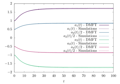
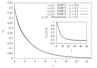
Figure 7: Comparison between discretized DMFT and GD dynamics for the Gaussian model (labeled as ‘Simulations’). GD results are averaged over $N=10^{4}$ realizations of the Gaussian process, under Setting 1 described in the main text. Left frame: Second layer for DMFT and GD with $\eta_{\mbox{\tiny\rm GD}}=\eta=0.1$. Right frame: Train error and correlation function for DMFT with a few values of $\eta$, and for GD.

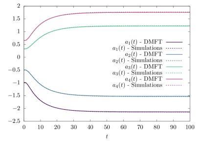
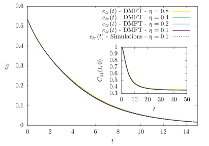
Figure 8: Comparison between discretized DMFT and GD dynamics (labeled as ‘Simulations’). GD results are averaged over $N=10^{4}$ realizations of the Gaussian process, under Setting 2 described in the main text. Results for GD are averaged over $N=10^{4}$ samples.

Setting 1.

We assume pure noise data with $\tau=1$ and train a network with $m=4$ neurons and covariance structure given by $h(z)=z/10+z^{2}/2$. We simulate GD trajectories, according to Eq. (C.9) with $d=100$, $n=150$, and correspondingly evaluate the Euler discretization of DMFT, cf. Section C.1 for $\overline{\alpha}=n/d=1.5$.

We choose an initialization that is not symmetric and therefore we have to use the full DMFT equations of Section B.1. More precisely, we initialize second layer weights as follows:

$$a_{1}(0)=a_{2}(0)=1\ \ \ \ \ a_{3}(0)=a_{4}(0)=-1$$ (C.12)

The weights of the first layer are instead initialized by generating two random vectors ${\boldsymbol{y}}_{1},\ {\boldsymbol{y}}_{2}\sim{\sf Unif}({\mathbb{S}}^{d-1})$, and setting

$${\boldsymbol{w}}_{1}(0)={\boldsymbol{w}}_{3}(0)={\boldsymbol{y}}_{1}\ \ \ \ \ {\boldsymbol{w}}_{2}(0)={\boldsymbol{w}}_{4}(0)={\boldsymbol{y}}_{2}$$ (C.13)

This initialization results in initializing the DMFT equations with

$$\begin{split}&C_{11}(0,0)=C_{22}(0,0)=C_{33}(0,0)=C_{44}(0,0)=1\,,\\ &C_{13}(0,0)=C_{24}(0,0)=1\,,\\ &C_{12}(0,0)=C_{14}(0,0)=C_{23}(0,0)=C_{34}(0,0)=0\,.\end{split}$$ (C.14)

Both for the discretized DMFT and for GD for several values of the stepsize. The results of this analysis are plotted in Fig. 7.

Setting 2.

We consider again pure noise with $\tau=1$, a network with $m=4$, input dimension $d=100$ and sample size $n=150$. We use hidden neurons with the same covariance structure as in the Setting 1.

However, we change the initialization with respect to Setting 1. First layer are initialized independently and uniformly at random. It follows that

$$C_{ij}(0,0)=\delta_{ij}\ \ \ \forall i,j=1,\ldots,4$$ (C.15)

Second layer weights are initialized according to

$$a_{1}(0)=-1\,,\ \ \ a_{2}(0)=-\frac{1}{2}\,,\ \ \ a_{3}(0)=\frac{1}{3}\,,\ \ \ a_{4}(0)=\frac{2}{3}\,.$$ (C.16)

We use stepsize $\eta=0.1$.

C.4 Construction of the Gaussian process $f^{g}(\,\cdot\,)$

The Gaussian process $f^{g}$ can be constructed as follows. Define a sequence of independent Gaussian tensors $\boldsymbol{J}^{(k)}\in({\mathbb{R}}^{d})^{\otimes k}$, $k\geq 1$, with entries $(J^{(k)}_{i_{1},\ldots,i_{k}}:i_{j}\leq d)\sim_{iid}{\sf N}(0,1)$. We then let

$$f^{g}({\boldsymbol{a}},\boldsymbol{W})=\frac{1}{m}\sum_{i=1}^{m}a_{i}\sum_{k=0}^{\infty}c_{k}\sum_{i_{1},\ldots,i_{k}=1}^{d}J^{(k)}_{i_{1},\ldots,i_{k}}w_{i,i_{1}}\ldots w_{i,i_{k}}$$ (C.17)

It is easy to check that this stochastic process has the prescribed covariance, with

$$h(z)=\sum_{k=0}^{\infty}c_{k}^{2}z^{k}\,,$$ (C.18)

has long as the series above has radius of convergence larger than $1$. An analogous construction holds for $\varphi^{g}$.

Appendix D Dynamical regimes: General preliminaries

In the next two sections, we will study the SymmDMFT equations of Section B.4 and characterize different dynamical regimes in the large network limit. From a technical viewpoint, we develop a singular perturbation theory of the DMFT equations as $m\to\infty$ for fixed overparametrization ratio $\alpha=\overline{\alpha}/m$.

While singular perturbation theory is a classical domain of mathematics [Ber01, Hol13], making this type of analysis rigorous is notoriously challenging. We will proceed heuristically as follows: $(i)$ Hypothesize a certain asymptotic behavior of the DMFT solution in a specific time-scale; $(ii)$ Check consistency with the DMFT equations; $(iii)$ Check that this behavior is observed in the numerical solution of the DMFT equations.

More precisely, a specific dynamical regime is identified by a scaling of the time variable, which in our case will take the form $t=t_{\#}(m)\cdot\hat{t}$ for a certain fixed function $t_{\#}(m)$ and $\hat{t}$ a scaled time of order one. The asymptotics of DMFT quantities in that regime takes the form (for instance)

$$\lim_{m\to\infty}\frac{1}{c_{\#}(m)}C_{o}\Big{(}t_{\#}(m)\cdot\hat{t},t_{\#}(m)\cdot\hat{s};m,\overline{\alpha}=\frac{\alpha}{m}\Big{)}=c_{o}(\hat{t},\hat{s};\alpha)\,,$$ (D.1)

where $c_{\#}(m)$, $c_{o}(\hat{t},\hat{s};\alpha)$ are two fixed functions, the limit is understood to hold at fixed $\hat{t},\hat{s},\alpha\in(0,\infty)$, and we made explicit the dependence of $C_{o}$ on $m$, $\overline{\alpha}$. More concisely, we will often write the above formula as

$$C_{o}\Big{(}t_{\#}(m)\cdot\hat{t},t_{\#}(m)\cdot\hat{s};m,\overline{\alpha}=\frac{\alpha}{m}\Big{)}=c_{\#}(m)c_{o}(\hat{t},\hat{s};\alpha)+o(c_{\#}(m))\,,$$ (D.2)

and we will typically use $t$, $s$ instead of $\hat{t}$, $\hat{s}$ for the dummy variables.

The behavior of the DMFT equations depends in a crucial way in the initialization of the second layer weights:

• In Section E, we will consider the case of a ‘lazy initialization,’ i.e. we will assume $a(0)=\gamma_{0}\sqrt{m}$ for some constant $\gamma_{0}\in(0,\infty)$ independent of $m$.

• In Section F, we will consider the ‘mean field initialization’ i.e. assume $a(0)=a_{0}$ to be constant and independent of $m$.

Appendix E Dynamical regimes: Lazy initialization

As anticipated, in this section we study dynamical regimes under lazy initialization. In subsection E.1, we will consider the case of pure noise data and in subsection E.2 the $k$-index model.

Throughout this section, we let $\gamma(t)=a(t)/\sqrt{m}$ (in particular, $\gamma(0)=\gamma_{0}$).

E.1 Pure noise model

Under the pure noise model, we have $\varphi=\hat{\varphi}=0$. Further, the variable ${\boldsymbol{v}}(t)$ is not defined and can be dropped (equivalently, we can set ${\boldsymbol{v}}(t)={\mathbf{0}}$).

We identify three dynamical regimes:

1. $t=O(1/m)$: $\gamma(t)=\gamma_{0}+o_{m}(1)$, train error decreases, and the network approximates the null function (Section E.1.1).

2. $t=\Theta(1)$: $\gamma(t)=\gamma_{0}+o_{m}(1)$, first-layer weights move significantly and train error converges to a limit $e_{*}(\gamma_{0})$ (Section E.1.2). If $\gamma_{0}$ is larger than the interpolation threshold, then train error vanishes in this regime.

3. $t=\Theta(m)$: This regime emerges only if $\gamma_{0}$ is smaller than the interpolation threshold. (We discuss the identification of the interpolation transition of gradient flow in Section E.1.3.)

   If this is the case, $\gamma(t)$ grows on the time scale $t=\Theta(m)$ until it crosses the interpolation threshold. At that point the train error vanishes (Section E.1.4).

Since in the first two regimes $\gamma(t)$ does not change appreciably, the dynamics in these time scales is essentially equivalent to the one of a network in which second-layer weights are fixed and do not evolve by GF. In Section E.1.1 and E.1.2 we first consider this case.

We note that the pure noise model is unchanged if we rescale $\tau\to c\tau$, $\gamma_{0}\to c\gamma_{0}$. More precisely, this results in a rescaling of the risk by $c^{2}$ and hence of time by the same factor. As a consequence quantities of interest often depend on $\gamma,\tau$ uniquely through their ratio $\gamma/\tau$.

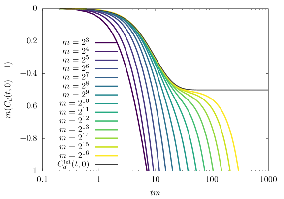
Figure 9: Rescaled correlation function $m(C_{d}(t,s)-1)$ in the first dynamical regime as a function of the scaled time $tm$ for a model initialized with a lazy scaling and fixed second layer weights. Different curves correspond to the numerical integration of the SymmDMFT equations at various values of $m$. They appear to converge to the scaling solution in the large $m$ limit described by Eqs. (E.6). Here $\alpha=0.5$, $\tilde{h}(z)=(3/10)z+z^{2}/2$ and $\tau=1$.

E.1.1 First dynamical regime: $t=O(1/m)$

We first consider the case in which the (scaled) second layer weights are not updated and fixed to their initialization, i.e. $\gamma(t)=\gamma_{0}$.

It is possible to check that, up to higher-order terms, the SymmDMFT equations are solved by functions of the form (the first equation holds in weak sense, i.e. after integrating against a test function)

$$R_{A}(t/m,s/m) =m\,\delta(t-s)+o_{m}(m) C_{A}(t/m,s/m) ={C}^{\mbox{\tiny\rm lz1}}_{A}(t,s)+o_{m}(1)$$ (E.1)

$$R_{o}(t/m,s/m) =\frac{1}{m}{R}^{\mbox{\tiny\rm lz1}}_{o}(t,s)+o_{m}(1/m) C_{o}(t/m,s/m) =\frac{1}{m}{C}^{\mbox{\tiny\rm lz1}}_{o}(t,s)+o_{m}(1/m)$$ (E.2)

$$R_{d}(t/m,s/m) =\vartheta(t-s)+o_{m}(1) C_{d}(t/m,s/m) =1+\frac{1}{m}{C}^{\mbox{\tiny\rm lz1}}_{d}(t,s)+o_{m}(1/m)$$ (E.3)

$$\nu(t/m) ={\nu}^{\mbox{\tiny\rm lz1}}(t)+o_{m}(1)\>.$$ (E.4)

where ${C}^{\mbox{\tiny\rm lz1}}_{A}$, ${C}^{\mbox{\tiny\rm lz1}}_{d}$, ${C}^{\mbox{\tiny\rm lz1}}_{o}$, ${\nu}^{\mbox{\tiny\rm lz1}}$ and ${R}^{\mbox{\tiny\rm lz1}}_{o}$ are suitable functions independent of $m$. Here and below, we use the notation $\vartheta(t)={\boldsymbol{1}}(t>0)$.

Note that Eq. (E.3) implies that on this dynamical regime the weights of the first layer change by order $1/m$.

Plugging the asymptotic form in Eqs. (E.1) to (E.4) into the SymmDMFT equations and matching the leading orders for large $m$, we obtain that the functions ${C}^{\mbox{\tiny\rm lz1}}_{A}$, ${C}^{\mbox{\tiny\rm lz1}}_{d}$, ${C}^{\mbox{\tiny\rm lz1}}_{o}$, ${\nu}^{\mbox{\tiny\rm lz1}}$ and ${R}^{\mbox{\tiny\rm lz1}}_{o}$ must satisfy

$$\begin{split}{\nu}^{\mbox{\tiny\rm lz1}}(t)&=-\alpha\gamma_{0}^{2}h^{\prime}(1)-\alpha\gamma_{0}^{2}h^{\prime}(0){C}^{\mbox{\tiny\rm lz1}}_{o}(t,t)\,,\\ \partial_{t}{R}^{\mbox{\tiny\rm lz1}}_{o}(t,t^{\prime})&=-\alpha\gamma_{0}^{2}h^{\prime}(0)\left(1+{R}^{\mbox{\tiny\rm lz1}}_{o}(t,t^{\prime})\right)\,,\\ \partial_{t}{C}^{\mbox{\tiny\rm lz1}}_{o}(t,t^{\prime})&=-\alpha\gamma_{0}^{2}h^{\prime}(0)\left(1+{C}^{\mbox{\tiny\rm lz1}}_{o}(t,t^{\prime})\right)\,,\\ \partial_{t}{C}^{\mbox{\tiny\rm lz1}}_{d}(t,t^{\prime})&=\alpha\gamma_{0}^{2}h^{\prime}(0)\left({C}^{\mbox{\tiny\rm lz1}}_{o}(t,t)-{C}^{\mbox{\tiny\rm lz1}}_{o}(t,t^{\prime})\right)\,,\\ {C}^{\mbox{\tiny\rm lz1}}_{A}(t,s)&=-\left[\tau^{2}+\gamma_{0}^{2}h(1)-\gamma_{0}^{2}h(0){C}^{\mbox{\tiny\rm lz1}}_{o}(t,s)\right]\>.\end{split}$$ (E.5)

These are a set of ordinary differential equations that can be solved explicitly. We get

$$\begin{split}{R}^{\mbox{\tiny\rm lz1}}_{o}(t,t^{\prime})&=\vartheta(t-t^{\prime})\left[e^{-\alpha\gamma_{0}^{2}h^{\prime}(0)(t-t^{\prime})}-1\right]\,,\\ {C}^{\mbox{\tiny\rm lz1}}_{o}(t,t)&=e^{-2\alpha\gamma_{0}^{2}h^{\prime}(0)t}-1\,,\\ {C}^{\mbox{\tiny\rm lz1}}_{o}(t,t^{\prime})&=-1+e^{-\alpha\gamma_{0}^{2}h^{\prime}(0)(t-t^{\prime})}({C}^{\mbox{\tiny\rm lz1}}_{o}(t^{\prime},t^{\prime})+1)\,\;\;\;\;\;\;\mbox{ for }t>t^{\prime}\,,\\ {C}^{\mbox{\tiny\rm lz1}}_{d}(t,t^{\prime})&=1+e^{-\alpha\gamma_{0}^{2}h^{\prime}(0)(t+t^{\prime})}-\frac{1}{2}\left(e^{-2\alpha\gamma_{0}^{2}h^{\prime}(0)t}+e^{-2\alpha\gamma_{0}^{2}h^{\prime}(0)t^{\prime}}\right)\,,\;\;\;\;\;\;\mbox{ for }t>t^{\prime}\>.\end{split}$$ (E.6)

In particular, Eqs. (E.6) imply

$$\begin{split}\lim_{t\to\infty}{C}^{\mbox{\tiny\rm lz1}}_{o}(t,t)&=-1\,,\\ \lim_{t,t^{\prime}\to\infty,\,t-t^{\prime}\to\infty}{R}^{\mbox{\tiny\rm lz1}}_{o}(t,t^{\prime})&=-1\>.\end{split}$$ (E.7)

Recalling Eq. (E.2) we conclude that

$$\lim_{t\to\infty}\lim_{m\to\infty}m\,C_{o}(t/m,t/m) =-1\,,$$ (E.8)

or, using the interpretation of $C_{o}$,

$$\lim_{t\to\infty}\lim_{m\to\infty}\lim_{n\to\infty}m\cdot\langle{\boldsymbol{w}}_{i}(t/m),{\boldsymbol{w}}_{j}(t/m)\rangle =-1\;\;\;\;\forall i\neq j\>.$$ (E.9)

In other words, at the end of this dynamical regime, the first-layer weights form a regular simplex, with center $\overline{{\boldsymbol{w}}}(t/m):=m^{-1}\sum_{i=1}^{m}{\boldsymbol{w}}_{i}(t/m)$ satisfying $\|\overline{{\boldsymbol{w}}}(t/m)\|^{2}=o_{m}(1)$.

Hence, at the end of the first dynamical regime, the first-layer weights are such that the linear component of the activation function $\sigma$ is removed. In other words, for $t$ a large constant, we have

$$f^{g}(\,\cdot\,;{\boldsymbol{a}}(t/m),\boldsymbol{W}(t/m))=\frac{\gamma_{0}}{\sqrt{m}}\sum_{i=1}^{m}\sigma^{\mbox{\rm\footnotesize nl}}_{G}({\boldsymbol{w}}_{i}(t/m))+{\rm err}\,,$$ (E.10)

where $\sigma^{\mbox{\rm\footnotesize nl}}_{G}({\boldsymbol{w}})$ is a Gaussian process with covariance structure given by $h(z)-zh^{\prime}(0)$, and ${\rm err}$ is small in mean square.

Notice also that this is achieved by a $O(1/\sqrt{m})$ change in each of the first layer weights. Indeed, by Eq. (E.3), we have

$$\lim_{n\to\infty}\|{\boldsymbol{w}}_{i}(0)-{\boldsymbol{w}}_{i}(t/m)\|^{2}=2-2C_{d}(0,t/m)=-\frac{2}{m}{C}^{\mbox{\tiny\rm lz1}}_{d}(0,t)+o_{m}(1/m)\,.$$ (E.11)

Equations (E.1) to (E.4) can be used to compute the behavior of the train error in this dynamical regime:

$$\lim_{m\to\infty}e_{\mbox{{\rm\footnotesize tr}}}(t/m)={e}^{\mbox{\tiny\rm lz1}}_{\mbox{{\rm\footnotesize tr}}}(t)\,.$$ (E.12)

Using Eqs. (E.6), we get the expression:

$${e}^{\mbox{\tiny\rm lz1}}_{\mbox{{\rm\footnotesize tr}}}(t)=\frac{1}{2}\left[\tau^{2}+\gamma_{0}^{2}h(1)+\gamma_{0}^{2}h^{\prime}(0){C}^{\mbox{\tiny\rm lz1}}_{o}(t,t)\right]\>.$$ (E.13)

In particular, the train error at the end of this dynamical regime is

$$\lim_{t\to\infty}\lim_{m\to\infty}e_{\mbox{{\rm\footnotesize tr}}}(t/m)=\lim_{t\to\infty}{e}^{\mbox{\tiny\rm lz1}}_{\mbox{{\rm\footnotesize tr}}}(t)=\frac{1}{2}\left[\tau^{2}+\gamma_{0}^{2}h(1)-\gamma_{0}^{2}h^{\prime}(0)\right]\,.$$ (E.14)

This is in agreement with (E.10). Indeed, note that

$$\widehat{\mathscrsfs{R}}_{n}({\boldsymbol{a}},\boldsymbol{W})=\frac{1}{2n}\|{\boldsymbol{{\varepsilon}}}\|^{2}-\frac{1}{n}\langle{\boldsymbol{{\varepsilon}}},{\boldsymbol{f}}^{g}({\boldsymbol{a}},\boldsymbol{W})\rangle+\frac{1}{2n}\|{\boldsymbol{f}}^{g}({\boldsymbol{a}},\boldsymbol{W})\|^{2}\,.$$ (E.15)

Training in this timescale attempts to minimize $\|{\boldsymbol{f}}^{g}({\boldsymbol{a}},\boldsymbol{W})\|^{2}$ without fitting the noise.

This picture is confirmed by the fact that Eqs. (E.6) depend on $h$ only through $h^{\prime}(0)$. This means that the dynamics on timescales of order $1/m$ is controlled by the linear part of the covariance structure of the hidden layer.

In Fig.9 we test the correctness of the asymtotic ansatz of Eqs. (E.1) to (E.4). Namely, we compare the results of numerical integration of the SymmDMFT equations for various values of $m$, with the prediction of Eqs. (E.6). The match is excellent.

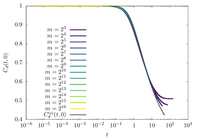
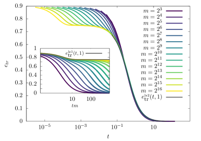
Figure 10: Training with pure noise data under lazy initialization: second dynamical regime $t=\Theta(1)$. Left panel: First-layer weights correlation function $C_{d}(t,0)$ measuring the inner product between neurons at time $0$ and time $t$, plotted versus $t$ for several values of $m$, and compared with the large $m$-asymptotics ${C}^{\mbox{\tiny\rm lz2}}_{d}$. Right panel: training error a $e_{\mbox{{\rm\footnotesize tr}}}(t,\gamma_{0},m)$ plotted versus $t$ for several values of $m$, and compared with the large-$m$ asymptotics in this regime ${e}^{\mbox{\tiny\rm lz2}}_{\mbox{{\rm\footnotesize tr}}}(t,1)$. Notice the two-steps decrease of the training error, corresponding to the two regimes $t=O(1/m)$ and $t=\Theta(1)$. Inset: Same curves plotted versus $tm$, and compared with the asymptotic prediction ${e}^{\mbox{\tiny\rm lz1}}_{\mbox{{\rm\footnotesize tr}}}(\,\cdot\,,1)$ in the first dynamical regime. For both panels we use $\alpha=0.5$, $\tilde{h}(z)=(3/10)z+z^{2}/2$, $\gamma_{0}=1$ and $\tau=1$.

So far we assumed that second-layer weights are not optimized and $\gamma(t)=\gamma_{0}$. What happens if drop this constraint? It can be checked that the form given in Eqs. (E.1)-(E.4) still solves the SymmDMFT equations when $a(t)$ is allowed to evolve, and $\gamma(t/m)=\gamma_{0}+o_{m}(1)$ for all fixed $t\in(0,\infty)$. In other words, second layer weights do not change significantly during this dynamical regime.

E.1.2 Second dynamical regime: $t=\Theta(1)$

The second dynamical regime arises when $t=\Theta(1)$. Recall from the previous subsection that, for $t=o_{m}(1)$, the train error remains close (for large $m$) to the plateau characterized at the end of the first dynamical regime, see Eq. (E.14). When $t$ is of order one, the first layer weights start changing by an amount of order one as well, and the model starts to fit the noise.

As before, we begin by considering the simplified setting in which $\gamma(t)=\gamma_{0}$ is fixed and not optimized by GF.

We claim that the SymmDMFT equations are solved by the following ansatz, up to lower order terms as $m\to\infty$:

$$\nu(t) ={\nu}^{\mbox{\tiny\rm lz2}}(t)+o_{m}(1)\,,$$ (E.16)

$$C_{d}(t,t^{\prime}) ={C}^{\mbox{\tiny\rm lz2}}_{d}(t,t^{\prime})+o_{m}(1)\,,$$ (E.17)

$$R_{d}(t,t^{\prime}) ={R}^{\mbox{\tiny\rm lz2}}_{d}(t,t^{\prime})+o_{m}(1)\,,$$ (E.18)

$$C_{o}(t,t^{\prime}) =\frac{1}{m}{C}^{\mbox{\tiny\rm lz2}}_{o}(t,t^{\prime})+o_{m}(1/m)=-\frac{1}{m}{C}^{\mbox{\tiny\rm lz2}}_{d}(t,t^{\prime})+o_{m}(1/m)\,,$$ (E.19)

$$R_{o}(t,t^{\prime}) =\frac{1}{m}{R}^{\mbox{\tiny\rm lz2}}_{o}(t,t^{\prime})+o_{m}(1/m)=-\frac{1}{m}{R}^{\mbox{\tiny\rm lz2}}_{d}(t,t^{\prime})+o_{m}(1/m)\,.$$ (E.20)

Here ${C}^{\mbox{\tiny\rm lz2}}_{d}$, ${R}^{\mbox{\tiny\rm lz2}}_{d}$, ${C}^{\mbox{\tiny\rm lz2}}_{o}$, ${R}^{\mbox{\tiny\rm lz2}}_{o}$ and ${\nu}^{\mbox{\tiny\rm lz2}}$ are certain functions independent of $m$. Equations (E.19),  (E.20) state in particular that ${C}^{\mbox{\tiny\rm lz2}}_{o}(t,t^{\prime})=-{C}^{\mbox{\tiny\rm lz2}}_{d}(t,t^{\prime})$ and ${R}^{\mbox{\tiny\rm lz2}}_{o}(t,t^{\prime})=-{R}^{\mbox{\tiny\rm lz2}}_{d}(t,t^{\prime})$, and the therefore we are left with the task of determining ${C}^{\mbox{\tiny\rm lz2}}_{d}(t,t^{\prime})$, ${R}^{\mbox{\tiny\rm lz2}}_{d}(t,t^{\prime})$. By substituting Eqs. (E.16) to (E.20) into the SymmDMFT equations and matching leading order terms, we get a set of two integral-differential equations for ${C}^{\mbox{\tiny\rm lz2}}_{d}(t,t^{\prime})$, ${R}^{\mbox{\tiny\rm lz2}}_{d}(t,t^{\prime})$, which we next state.

We first define

$$\begin{split}{\Sigma}^{\mbox{\tiny\rm lz2}}_{R}(t,s)&:=\gamma_{0}^{2}\left(h^{\prime}({C}^{\mbox{\tiny\rm lz2}}_{d}(t,s))-h^{\prime}(0)\right){R}^{\mbox{\tiny\rm lz2}}_{d}(t,s)\,,\\ {\Sigma}^{\mbox{\tiny\rm lz2}}_{C}(t,s)&:=\tau^{2}+\gamma_{0}^{2}h({C}^{\mbox{\tiny\rm lz2}}_{d}(t,s))-\gamma_{0}^{2}h^{\prime}(0){C}^{\mbox{\tiny\rm lz2}}_{d}(t,s)\,,\end{split}$$ (E.21)

then we define ${R}^{\mbox{\tiny\rm lz2}}_{A}$ and ${C}^{\mbox{\tiny\rm lz2}}_{A}$ as the solution of

$$\begin{split}\delta(t-t^{\prime})&=\int_{t^{\prime}}^{t}\left[\delta(t-s)+{\Sigma}^{\mbox{\tiny\rm lz2}}_{R}(t,s)\right]{R}^{\mbox{\tiny\rm lz2}}_{A}(s,t^{\prime})\,{\rm d}s\,,\\ 0&=\int_{0}^{t}\left[\delta(t-s)+{\Sigma}^{\mbox{\tiny\rm lz2}}_{R}(t,s)\right]{C}^{\mbox{\tiny\rm lz2}}_{A}(s,t^{\prime}){\rm d}s+\int_{0}^{t^{\prime}}{\Sigma}^{\mbox{\tiny\rm lz2}}_{C}(t,s){R}^{\mbox{\tiny\rm lz2}}_{A}(t^{\prime},s)\,{\rm d}s\>.\end{split}$$ (E.22)

We next define the asymptotic form for the memory kernels

$$\begin{split}{M}^{\mbox{\tiny\rm lz2}}_{R}(t,s)&:=\alpha\left[{R}^{\mbox{\tiny\rm lz2}}_{A}(t,s)\tilde{h}^{\prime}({C}^{\mbox{\tiny\rm lz2}}_{d}(t,s))+{C}^{\mbox{\tiny\rm lz2}}_{A}(t,s)\tilde{h}^{\prime\prime}({C}^{\mbox{\tiny\rm lz2}}_{d}(t,s)){R}^{\mbox{\tiny\rm lz2}}_{d}(t,s)\right]\,,\\ {M}^{\mbox{\tiny\rm lz2}}_{C}(t,s)&:=\alpha\tilde{h}^{\prime}({C}^{\mbox{\tiny\rm lz2}}_{d}(t,s)){C}^{\mbox{\tiny\rm lz2}}_{A}(t,s)\,.\end{split}$$ (E.23)

and we have defined

$$\tilde{h}(z):=h(z)-h^{\prime}(0)z\>.$$ (E.24)

The equations for ${\nu}^{\mbox{\tiny\rm lz2}}$, ${C}^{\mbox{\tiny\rm lz2}}_{d}$ and ${R}^{\mbox{\tiny\rm lz2}}_{d}$ are then given by

$${\nu}^{\mbox{\tiny\rm lz2}}(t)=-\int_{0}^{t}\left[{M}^{\mbox{\tiny\rm lz2}}_{R}(t,s){C}^{\mbox{\tiny\rm lz2}}_{d}(t,s)+{M}^{\mbox{\tiny\rm lz2}}_{C}(t,s){R}^{\mbox{\tiny\rm lz2}}_{d}(t,s)\right]\,{\rm d}s\,,$$ (E.25)

$$\partial_{t}{R}^{\mbox{\tiny\rm lz2}}_{d}(t,t^{\prime})=\delta(t-t^{\prime})-{\nu}^{\mbox{\tiny\rm lz2}}(t){R}^{\mbox{\tiny\rm lz2}}_{d}(t,t^{\prime})-\int_{t^{\prime}}^{t}{M}^{\mbox{\tiny\rm lz2}}_{R}(t,s){R}^{\mbox{\tiny\rm lz2}}_{d}(s,t^{\prime})\,{\rm d}s\,,$$ (E.26)

$$\partial_{t}{C}^{\mbox{\tiny\rm lz2}}_{d}(t,t^{\prime})=-{\nu}^{\mbox{\tiny\rm lz2}}(t){C}^{\mbox{\tiny\rm lz2}}_{d}(t,t^{\prime})-\int_{0}^{t}{M}^{\mbox{\tiny\rm lz2}}_{R}(t,s){C}^{\mbox{\tiny\rm lz2}}_{d}(t^{\prime},s)\,{\rm d}s-\int_{0}^{t^{\prime}}{M}^{\mbox{\tiny\rm lz2}}_{C}(t,s){R}^{\mbox{\tiny\rm lz2}}_{d}(t^{\prime},s)\,{\rm d}s\>.$$ (E.27)

(As before, in the second and last equation, it is understood that $t\geq t^{\prime}$, and the last equation is understood to hold in weak sense.)

Given the constraints on $C_{d}$, $R_{d}$, we have the following constraints on ${C}^{\mbox{\tiny\rm lz2}}_{d}$, ${R}^{\mbox{\tiny\rm lz2}}_{d}$,

$${C}^{\mbox{\tiny\rm lz2}}_{d}(t,t) =1\,,$$ (E.28)

$${C}^{\mbox{\tiny\rm lz2}}_{d}(t,s) ={C}^{\mbox{\tiny\rm lz2}}_{d}(s,t)\,,$$ (E.29)

$${R}^{\mbox{\tiny\rm lz2}}_{d}(t,s) =0\;\;\;\;\;\forall t\leq s\,.$$ (E.30)

In particular, the last condition, together with Eq. (E.26) implies ${R}^{\mbox{\tiny\rm lz2}}_{d}(t+,t)=1$.

The evolution of the the train error in this second dynamical regime is given by

$$\lim_{m\to\infty}e_{\mbox{{\rm\footnotesize tr}}}(t) ={e}^{\mbox{\tiny\rm lz2}}_{\mbox{{\rm\footnotesize tr}}}(t,\gamma_{0})\,,$$ (E.31)

$${e}^{\mbox{\tiny\rm lz2}}_{\mbox{{\rm\footnotesize tr}}}(t,\gamma_{0}) =-\frac{1}{2}{C}^{\mbox{\tiny\rm lz2}}_{A}(t,t)\>,$$ (E.32)

where we have made explicit the dependence on the initialization of second-layer weights $\gamma_{0}$.

Note that Eq. (E.22) implies ${C}^{\mbox{\tiny\rm lz2}}_{A}(0,0)=-{\Sigma}^{\mbox{\tiny\rm lz2}}_{C}(0,0)$, and Eq. (E.21) yields ${\Sigma}^{\mbox{\tiny\rm lz2}}_{C}(0,0)=\tau^{2}+\gamma_{0}^{2}h(1)-\gamma_{0}^{2}h^{\prime}(0)$. Therefore

$$\lim_{t\to 0}{e}^{\mbox{\tiny\rm lz2}}_{\mbox{{\rm\footnotesize tr}}}(t,\gamma_{0})=\frac{1}{2}\left[\tau^{2}+\gamma_{0}^{2}\tilde{h}(1)\right]=\lim_{t\to\infty}{e}^{\mbox{\tiny\rm lz1}}_{\mbox{{\rm\footnotesize tr}}}(t,\gamma_{0})\,.$$ (E.33)

In other words, this second dynamical regime captures the decrease of the training error which starts at the plateau reached in the first regime, cf. Eq. (E.14). which coincides with the long time extrapolation of the first dynamical regime.

This second dynamical regime is fully non-linear and depends on the entire covariance function $\tilde{h}$. Further, the first order weights move by an amount $\|{\boldsymbol{w}}_{i}(t)-{\boldsymbol{w}}_{i}(0)\|=\Theta(1)$, as follows from the fact that ${C}^{\mbox{\tiny\rm lz2}}_{d}(t,0)<1$ strictly.

In order to confirm the ansatz (E.16) to (E.20), we compared the solution of the full SymmDMFT equations, with the solution of the asymptotic equations (E.25), (E.27). An example of such a comparison is presented in Fig. 10: the agreement is excellent.

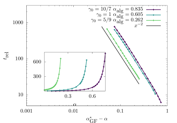
Figure 11: Training with pure noise data under lazy initialization. We plot the time for GF to converge to near-zero training error as a function of $\alpha$, for various values of $\gamma_{0}$, as computed using the theory of Section E.1.2. The divergence of $t_{\text{rel}}$ signals the phase transition for GF interpolation $\alpha_{\mbox{\tiny\rm GF}}^{*}$. Inset: $\tau_{\text{rel}}$ versus $\alpha$ in linear scale. Main panel: $t_{\text{rel}}$ versus $\alpha_{\mbox{\tiny\rm GF}}^{*}-\alpha$ (with the fitted value of $\alpha^{*}_{\mbox{\tiny\rm GF}}$). Here we use $h(z)=(3/10)z+z^{2}/2$.

The treatment above assumed the constraint $\gamma(t)=\gamma_{0}$. However, as in the first dynamical regime, if we let second layer weights evolve, they do not change appreciably. Namely, the asymptotic form given in Eqs. (E.16) to (E.20) still solves the SymmDMFT equations when $a(t)$ is allowed to evolve. We have $\gamma(t)=\gamma_{0}+o_{m}(1)$ on this timescale.

E.1.3 The algorithmic interpolation transition

For the discussion in this section, we denote by $e_{\mbox{{\rm\footnotesize tr}}}(t,\gamma_{0},m,\alpha)$ the train error as a function of $t$, where we emphasized the dependence on the initial condition $\gamma_{0}$, on the number of neurons $m$, and on the overparametrization ratio $\alpha$. We further assume that second layer weigths are not evolved and therefore $\gamma(t)=\gamma_{0}$ for all $t$. We define the asymptotic train error achieved by GF as

$$e_{\mbox{{\rm\footnotesize tr}},\infty}(\gamma_{0},m,\alpha) :=\lim_{t\to\infty}e_{\mbox{{\rm\footnotesize tr}}}(t,\gamma_{0},m,\alpha)$$ (E.34)

$$=\lim_{t\to\infty}\lim_{n\to\infty}\widehat{\mathscrsfs{R}}_{n}({\boldsymbol{a}},\boldsymbol{W}(t))\,.$$ (E.35)

Again, in this definition $a_{i}=\gamma_{0}\sqrt{m}$ is kept fixed and does not evolve with time.

Notice that it is in principle possible that $\lim_{n\to\infty}\widehat{\mathscrsfs{R}}_{n}({\boldsymbol{a}},\boldsymbol{W}(t_{n}))$ is strictly smaller than $e_{\mbox{{\rm\footnotesize tr}},\infty}(\gamma_{0},m,\alpha)$ if we let $t_{n}$ diverge with $n$ at sufficiently fast rate. However, based on results on related models in spin-glass theory we expect this not to be the case as long as $t_{n}$ is polynomial in $n$. Explicitly, we expect that, for any sequence $t_{n}\to\infty$

$$t_{n}\leq n^{C}\;\;\Rightarrow\;\;\lim_{n\to\infty}\widehat{\mathscrsfs{R}}_{n}({\boldsymbol{a}},\boldsymbol{W}(t_{n}))=e_{\mbox{{\rm\footnotesize tr}},\infty}(\gamma_{0},m,\alpha)\,.$$ (E.36)

Using the reduced equations for $t=\Theta(1)$ timescale, i.e. Eqs. (E.25) to (E.27), we can also define

$${e}^{\mbox{\tiny\rm lz2}}_{\mbox{{\rm\footnotesize tr}},\infty}(\gamma_{0},\alpha) :=\lim_{t\to\infty}{e}^{\mbox{\tiny\rm lz2}}_{\mbox{{\rm\footnotesize tr}}}(t,\gamma_{0},\alpha)$$ (E.37)

$$=\lim_{t\to\infty}\lim_{m\to\infty}\lim_{n\to\infty}\widehat{\mathscrsfs{R}}_{n}({\boldsymbol{a}},\boldsymbol{W}(t))\,.$$

A natural question is whether the large $m$ limit of $e_{\mbox{{\rm\footnotesize tr}},\infty}(\gamma_{0},m,\alpha)$ coincides with ${e}^{\mbox{\tiny\rm lz2}}_{\mbox{{\rm\footnotesize tr}},\infty}(\gamma_{0},\alpha)$. This amounts to asking whether there exists dynamical regime with timescale $t(m)$ diverging with $m$ at which $e_{\mbox{{\rm\footnotesize tr}}}(t(m),\gamma_{0},m,\alpha)$ starts diverging significantly from the value at the end of the second dynamical regime namely ${e}^{\mbox{\tiny\rm lz2}}_{\mbox{{\rm\footnotesize tr}},\infty}(\gamma_{0},\alpha)$. If ${e}^{\mbox{\tiny\rm lz2}}_{\mbox{{\rm\footnotesize tr}},\infty}(\gamma_{0},\alpha)=0$ then of course $\lim_{m\to\infty}e_{\mbox{{\rm\footnotesize tr}}}(t(m),\gamma_{0},m,\alpha)=0$ as well.

If however ${e}^{\mbox{\tiny\rm lz2}}_{\mbox{{\rm\footnotesize tr}},\infty}(\gamma_{0},\alpha)>0$, then the answer depends upon whether the second layer weights are evolved with GF:

• In the constrained setting in which second-layer weights do not evolve, we observe (from numerical solutions of ${\sf SymmDMFT}\,$) that

  $$\lim_{m\to\infty}e_{\mbox{{\rm\footnotesize tr}},\infty}(\gamma_{0},m,\alpha)={e}^{\mbox{\tiny\rm lz2}}_{\mbox{{\rm\footnotesize tr}},\infty}(\gamma_{0},\alpha)\,.$$ (E.38)

• In the next section we will see that if $\gamma(t)$ evolves with GF then the train error achieved on a diverging timescale $t=\Theta(m)$ is strictly smaller than ${e}^{\mbox{\tiny\rm lz2}}_{\mbox{{\rm\footnotesize tr}},\infty}(\gamma_{0},\alpha)$ and vanishes for large enough $t$.

Note that $e_{\mbox{{\rm\footnotesize tr}},\infty}(\gamma_{0},m,\alpha)$ and ${e}^{\mbox{\tiny\rm lz2}}_{\mbox{{\rm\footnotesize tr}},\infty}(\gamma_{0},\alpha)$ also depend on the noise variance $\tau^{2}$. However, because of the invariance under rescaling discussed at the beginning of this section (adding $\tau$ as an argument):

$${e}^{\mbox{\tiny\rm lz2}}_{\mbox{{\rm\footnotesize tr}},\infty}(\gamma_{0},\alpha,\tau^{2})=\tau^{2}\cdot{e}^{\mbox{\tiny\rm lz2}}_{\mbox{{\rm\footnotesize tr}},\infty}(\gamma_{0}/\tau,\alpha,\tau^{2}=1)\,,$$ (E.39)

and similarly for $e_{\mbox{{\rm\footnotesize tr}},\infty}(\gamma_{0},m,\alpha)$. Because of this relation, we can think that $\tau^{2}$ is fixed throughout, e.g. $\tau^{2}=1$.

We expect $e_{\mbox{{\rm\footnotesize tr}},\infty}(\gamma_{0},m,\alpha)$, ${e}^{\mbox{\tiny\rm lz2}}_{\mbox{{\rm\footnotesize tr}},\infty}(\gamma_{0},\alpha)$ to be non-increasing in $\gamma_{0}$, and define the thresholds

$$\gamma_{\mbox{\tiny\rm GF}}(\alpha,m) :=\inf\big{\{}\gamma_{0}:\;e_{\mbox{{\rm\footnotesize tr}},\infty}(\gamma_{0},m,\alpha)=0\big{\}}\,,$$ (E.40)

$$\gamma^{*}_{\mbox{\tiny\rm GF}}(\alpha) :=\inf\big{\{}\gamma_{0}:\;{e}^{\mbox{\tiny\rm lz2}}_{\mbox{{\rm\footnotesize tr}},\infty}(\gamma_{0},\alpha)=0\big{\}}\,.$$ (E.41)

(These definitions need to be modified if $\gamma_{0}\mapsto e_{\mbox{{\rm\footnotesize tr}},\infty}(\gamma_{0},m,\alpha)$ is non-monotone.)

Of course, Eq. (E.38) implies

$$\lim_{m\to\infty}\gamma_{\rm GF}(\alpha,m)=\gamma^{*}_{\rm GF}(\alpha)\,.$$ (E.42)

The numerical solution of the SymmDMFT equations imply that the curve $\gamma^{*}_{\mbox{\tiny\rm GF}}(\alpha)$ is monotone increasing with $\alpha$, as also suggested by the Gaussian complexity bound (see Section 2.2 in the main text). Hence we can invert it to get a threshold $\alpha_{\mbox{\tiny\rm GF}}^{*}(\gamma_{0})$: the two descriptions are equivalent.

In order to determine $\alpha_{\mbox{\tiny\rm GF}}^{*}(\gamma_{0})$, we adopt a procedure already implemented in [KU23a] for a simpler model. The procedure is based on the observation (from numerical solutions) that when ${e}^{\mbox{\tiny\rm lz2}}_{\mbox{{\rm\footnotesize tr}},\infty}(\gamma_{0},\alpha)=0$, ${e}^{\mbox{\tiny\rm lz2}}_{\mbox{{\rm\footnotesize tr}}}(t,\gamma_{0},\alpha)=\exp(-t/t_{\text{rel}}(\alpha;{\varepsilon})+o(t))$ for some $t_{\text{rel}}(\alpha)>0$ which diverges as $\alpha\uparrow\alpha_{\mbox{\tiny\rm GF}}$.

1. Define a grid of values of $\alpha$, $A_{0}=\{\alpha_{1},\alpha_{2},\dots,\alpha_{K}\}$, which are expected to be smaller than $\alpha_{\mbox{\tiny\rm GF}}^{*}(\gamma_{0})$.

2. For each value $\alpha\in A_{0}$, integrate numerically the reduced equations (E.25) to (E.27). Verify that ${e}^{\mbox{\tiny\rm lz2}}_{\mbox{{\rm\footnotesize tr}}}(t,\gamma_{0},\alpha)$ appear to converge to $0$ with $t\to\infty$. Let $A\subseteq A_{0}$ be the subset of values for which this happens.

3. For each $\alpha\in A$, define $t_{\text{rel}}(\alpha_{i};{\varepsilon}):=\inf\{t:{e}^{\mbox{\tiny\rm lz2}}_{\mbox{{\rm\footnotesize tr}}}(t,\gamma_{0},\alpha_{i})<{\varepsilon}\cdot\tau^{2}\}$ where ${\varepsilon}$ is a small threshold value (we use ${\varepsilon}=10^{-7}$).

4. Estimate parameters $\alpha^{*}_{\mbox{\tiny\rm GF}}(\gamma_{0}),c,\nu$ by fitting the relation $t_{\rm rel}(\alpha_{i};{\varepsilon})\sim c(\alpha^{*}_{\mbox{\tiny\rm GF}}-\alpha_{i})^{-\nu}$.

Figure 11 illustrates the calculation of $\alpha^{*}_{\mbox{\tiny\rm GF}}(\gamma_{0})$ for three values of $\gamma_{0}$. In the inset we plot $t_{\text{rel}}$ for three values of $\gamma_{0}$ as a function of $\alpha$. In the main panel, we demonstrate the divergence of $t_{\text{rel}}$ when $(\alpha^{*}_{\mbox{\tiny\rm GF}}-\alpha)$ vanishes. In practice, we observe $\nu=2$ fit well the data across a variety of settings, suggesting this is the universal exponent for the divergence of $t_{\text{rel}}$.

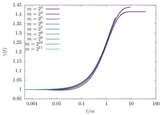
Figure 12: Training with pure noise data under lazy initialization: third dynamical regime. Evolution of the (rescaled) weights of the second layer as a function of $t/m$. Here $\tau=2.5$ and $\gamma_{0}=1$, $\alpha=0.3$, and covariance structure for the neurons given by $h(z)=(9/10)z+z^{2}/2$.

E.1.4 Third dynamical regime: $t=\Theta(m)$

In the first two dynamical regimes, the large-$m$ behavior did not depend on whether we would let second layer evolve with GF or we kept them fixed, i.e. $\gamma(t)=\gamma_{0}$.

In contrast, the behavior on timescales diverging with $m$ depends significantly on the dynamics of second-layer weights.

• If second layer weights are fixed, no significant further evolution takes place. In particular, the training error does not decrease significantly below the value reached at the end of the second dynamical regime, i.e. $e^{\ell}_{\mbox{{\rm\footnotesize tr}},\infty}(\gamma_{0},\alpha)$. This is stated formally in Eq. (E.38).

• If second layer weights evolve according to GF, then the dynamics on time-scales diverging with $m$ can be non-trivial and depends on the second-layer weights initialization $\gamma_{0}$. If $\gamma_{0}>\gamma_{\mbox{\tiny\rm GF}}^{*}(\alpha)$, then GR reaches vanishing training error during the second dynamical regime, and no further evolution takes place.

  However, if $\gamma_{0}<\gamma_{\mbox{\tiny\rm GF}}^{*}(\alpha)$, second layer weights start evolving when $t=\Theta(m)$, thus giving rise to a third dynamical regime. This is the object of the present subsection.

In Fig. 12, left frame, we plot the rescaled second layer weights $\gamma(t)$ (as predicted by numerical integration of the SymmDMFT equation) as a function of time for several values of $m$. Here, obviously, we do not constrain $\gamma(t)=\gamma(0)$.

We observe that $\gamma(t)$ changes only when $t=\Theta(m)$. Indeed, when plotted against $t/m$, curves obtained for different values of $m$ collapse onto each other. This suggests that, for $t=o(m)$ $\gamma(t)=\gamma(0)+o_{m}(1)$ (recall that $\gamma(0)=\gamma_{0}$ by definition). Further, the curve collapse suggests that, for any fixed $\hat{t}\in(0,\infty)$:

$$\lim_{m\to\infty}\gamma(\hat{t}\,m,\gamma_{0})={\gamma}^{\mbox{\tiny\rm lz3}}(\hat{t},\gamma_{0})\,,$$ (E.43)

where we have made explicit the dependence on $\gamma_{0}$. Of course, the case $\gamma_{0}>\gamma^{*}_{\mbox{\tiny\rm GF}}(\alpha)$ fits in this framework with ${\gamma}^{\mbox{\tiny\rm lz3}}(z,\gamma_{0})=\gamma_{0}$ identically.

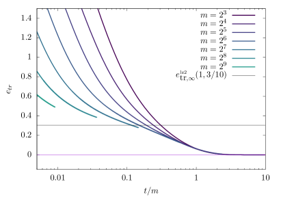
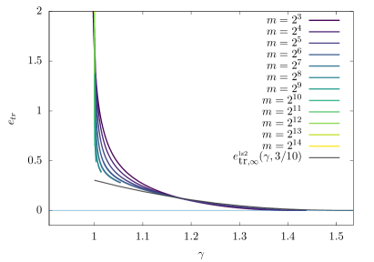
Figure 13: Training with pure noise data under lazy initialization: third dynamical regime. Left frame: Train error on timescales of order $m$. Right frame: GF trajectories in the plane $\gamma$ (second layer weights) — $e_{\mbox{{\rm\footnotesize tr}}}$ (train error). Black dots represent pairs $(\gamma,{e}^{\mbox{\tiny\rm lz2}}_{\mbox{{\rm\footnotesize tr}},\infty}(\gamma))$, where ${e}^{\mbox{\tiny\rm lz2}}_{\mbox{{\rm\footnotesize tr}},\infty}(\gamma)$ is the train error achieved at the end of the first dynamical regime, cf. Section E.1.3. The data has been produced from the same model as in Fig. 12.

We next consider the evolution of the train error. In Fig. 13, left frame, we plot the train error (again, as predicted by numerical integration of the SymmDMFT equation) as a function of time for several values of $m$.

Again, when plotted as a function of $t/m$, curves for different values of $m$ reach a plateau, and collapse below the plateau. This suggests the following limit behavior, which is consistent with Eq. (E.43)

$$\lim_{m\to\infty}\tilde{e}_{\mbox{{\rm\footnotesize tr}}}(\hat{t}\,m,\gamma_{0},m)={e}^{\mbox{\tiny\rm lz3}}_{\mbox{{\rm\footnotesize tr}}}(\hat{t},\gamma_{0})\>.$$ (E.44)

(Here we use $\tilde{e}_{\mbox{{\rm\footnotesize tr}}}(\hat{t}\,m,\gamma_{0})$ to denote the train error when second-layer weights evolve, in contrast with $e_{\mbox{{\rm\footnotesize tr}}}(\hat{t}\,m,\gamma_{0})$ which we used for the setting in which second-layer weights are constrained.)

Matching the present dynamical regime ($t=\Theta(m)$) with previous one ($t=\Theta(1)$, cf. Section E.1.2), implies that

$$\lim_{\hat{t}\to 0+}{e}^{\mbox{\tiny\rm lz3}}_{\mbox{{\rm\footnotesize tr}}}(\hat{t},\gamma_{0})=\lim_{t\to\infty}{e}^{\mbox{\tiny\rm lz2}}_{\mbox{{\rm\footnotesize tr}}}(t,\gamma_{0})={e}^{\mbox{\tiny\rm lz2}}_{\mbox{{\rm\footnotesize tr}},\infty}(\gamma_{0})$$ (E.45)

In other words, the function ${e}^{\mbox{\tiny\rm lz3}}_{\mbox{{\rm\footnotesize tr}}}$ describes the decrease of the train error below the level ${e}^{\mbox{\tiny\rm lz2}}_{\mbox{{\rm\footnotesize tr}},\infty}(\gamma_{0})$ achieved during the second dynamical regime.

In order to characterize the scaling function ${e}^{\mbox{\tiny\rm lz3}}_{\mbox{{\rm\footnotesize tr}}}$, in Fig. 13, right frame, we plot parametrically the the train error for different values of $m$ as a function of the second layer weights $\gamma(t)$. We also plot the curve $(\gamma,{e}^{\mbox{\tiny\rm lz2}}_{\mbox{{\rm\footnotesize tr}},\infty}(\gamma))$. This plot is consistent with the following behavior as $m\to\infty$. In a first regimes (corresponding to $t=o(m)$) the train error has a drop that becomes vertical in the $m\to\infty$ limit, implying that $\gamma(t)$ does not evolve while the train error decreases until it reaches $e_{\mbox{{\rm\footnotesize tr}},\infty}^{\ell}(\gamma_{0})$. In the last regime (corresponding to $t=\Theta(m)$), $\gamma(t)$ increases together with the decrease of the train error $e^{\ell}_{\mbox{{\rm\footnotesize tr}}}(t,\gamma_{0})$. Remarkably, they follow the curve $(\gamma,{e}^{\mbox{\tiny\rm lz2}}_{\mbox{{\rm\footnotesize tr}},\infty}(\gamma))$.

In order to describe the last regime, we point out that $t\mapsto{\gamma}^{\mbox{\tiny\rm lz3}}(t)$ is monotone increasing. Therefore we can re-parametrize time by the value of the second layer weights. Namely, define $\tilde{\gamma}^{-1}$ the inverse function, so that

$$\hat{t}=\tilde{\gamma}^{-1}({\gamma}^{\mbox{\tiny\rm lz3}}(\hat{t},\gamma_{0}),\gamma_{0})\>.$$ (E.46)

Using this reparametrization of time, the behavior in Fig. 13 can be formalized as

$$\lim_{t,m\to\infty:\gamma(t,\gamma_{0},m)=\tilde{\gamma}}{e}^{\mbox{\tiny\rm lz3}}_{\mbox{{\rm\footnotesize tr}}}(t,\gamma_{0},m)={e}^{\mbox{\tiny\rm lz3}}_{\mbox{{\rm\footnotesize tr}}}(\tilde{\gamma}^{-1}(\tilde{\gamma},\gamma_{0}),\gamma_{0})=:\varepsilon(\tilde{\gamma},\gamma_{0})\>.$$ (E.47)

The collapse on finite $m$ curves in Fig. 13, right frame, onto the curve $(\gamma,{e}^{\mbox{\tiny\rm lz2}}_{\mbox{{\rm\footnotesize tr}},\infty}(\gamma))$ suggests that

$$\gamma>\gamma_{0}\;\;\Rightarrow\;\;\varepsilon(\tilde{\gamma},\gamma_{0})={e}^{\mbox{\tiny\rm lz2}}_{\mbox{{\rm\footnotesize tr}},\infty}(\gamma)\>.$$ (E.48)

In other words, the dynamics on timescales of order $m$ is adiabatic: at each increase of $\gamma(t)$ on timescales of order $m$, the train error relaxes to the the value it would have had if the second layer weights would have been fixed in time at the corresponding value of $\gamma$.

A remarkable consequence of Eq. (E.48) is that that

$$\lim_{\hat{t}\to\infty}{\gamma}^{\mbox{\tiny\rm lz3}}(\hat{t})=\lim_{m\to\infty}\gamma_{\rm GF}(\alpha,m)=\gamma^{*}_{\rm GF}(\alpha)\>.$$ (E.49)

In words, in the large network limit, the norm of second-layer weights at the end of training is asymptotically the minimum norm that allows for interpolation.

E.2 Multi-index model

In this section we generalize the computations of Section E.1 to the case in which the dataset has a structure produced via a $k$-index model. The weights of the second layer are set to $a(t)=\gamma(t)\sqrt{m}$ and evolve with GF. The initialization scale $\gamma(0)=\gamma_{0}$ is fixed and independent of $m$.

As in the pure noise case, we identify three dynamical regimes:

1. $t=O(1/m)$: $\gamma(t)=\gamma_{0}+o_{m}(1)$, $\|{\boldsymbol{w}}_{i}(t)-{\boldsymbol{w}}_{i}(0)\|=\Theta(1/\sqrt{m})$. On this scale the network only learns a linear approximation of the target. Test and train error remain close to each other (Section E.2.1).

2. $t=\Theta(1)$: $\gamma(t)=\gamma_{0}+o_{m}(1)$, $\|{\boldsymbol{w}}_{i}(t)-{\boldsymbol{w}}_{i}(0)\|=\Theta(1)$. Test error does not change but train error decreases significantly (Section E.2.2).

3. $t=\Theta(m)$: This regime only emerges if $\gamma_{0}$ is below a certain interpolation threshold, i.e. $\gamma_{0}<\gamma_{\mbox{\tiny\rm GF}}^{*}(\alpha,\varphi,\tau)$. In this regime $\gamma(t)$ grows until the threshold, and train error decreases to $0$ while test error decreases to $0$ (Section E.2.5).

E.2.1 First dynamical regime: $t=O(1/m)$

On this timescale, the SymmDMFT equations are solved, up to higher order terms, by the following ansatz:

$$C_{d}(t/m,s/m) =1+o_{m}(1)\,, R_{d}(t/m,s/m) =\vartheta(t-s)+o_{m}(1)\,,$$ (E.50)

$$C_{o}(t/m,s/m) =\frac{1}{m}{C}^{\mbox{\tiny\rm lz1}}_{o}(t,s)+o_{m}(m^{-1})\,, R_{o}(t/m,s/m) =\frac{1}{m}{R}^{\mbox{\tiny\rm lz1}}_{o}(t,s)+o_{m}(m^{-1})\,,$$ (E.51)

$$\frac{1}{m}R_{A}(t/m,s/m) =\delta(t-s)+o_{m}(1)\,, C_{A}(t/m,s/m) =-{\Sigma}^{\mbox{\tiny\rm lz1}}_{C}(t,s)+o_{m}(1)\,,$$ (E.52)

$$a(t/m)\sqrt{m} =\gamma_{0}+o_{m}(1)\,, v(t/m) =\frac{1}{\sqrt{m}}{{\boldsymbol{v}}}^{\mbox{\tiny\rm lz1}}(t)+o_{m}(m^{-1/2})\,,$$ (E.53)

with

$${\Sigma}^{\mbox{\tiny\rm lz1}}_{C}(t,s)=\tau^{2}+\|\varphi\|^{2}-\gamma_{0}\langle\nabla\hat{\varphi}({\mathbf{0}}),{{\boldsymbol{v}}}^{\mbox{\tiny\rm lz1}}(t)\rangle-\gamma_{0}\langle\nabla\hat{\varphi}({\mathbf{0}}),{{\boldsymbol{v}}}^{\mbox{\tiny\rm lz1}}(s)\rangle+\gamma_{0}^{2}\left(h(1)+h^{\prime}(0){C}^{\mbox{\tiny\rm lz1}}_{o}(t,s)\right)\>.$$ (E.54)

In particular, Eq. (E.50) implies $\|{\boldsymbol{w}}_{i}(0)-{\boldsymbol{w}}_{i}(t/m)\|=o_{m}(1)$: weights of the first layer change by small amount.

The scaling functions defined in Eqs. (E.50)-(E.53) satisfy a set of equations that can be derived directly from the SymmDMFT equations:

$$\begin{split}\partial_{t}{{\boldsymbol{v}}}^{\mbox{\tiny\rm lz1}}(t)&=\alpha\gamma_{0}\nabla\hat{\varphi}({\mathbf{0}})-\alpha\gamma_{0}^{2}h^{\prime}(0){{\boldsymbol{v}}}^{\mbox{\tiny\rm lz1}}(t)\,,\\ \partial_{t}{C}^{\mbox{\tiny\rm lz1}}_{o}(t,t^{\prime})&=\alpha\gamma_{0}\langle\nabla\hat{\varphi}^{\prime}({\mathbf{0}}),{{\boldsymbol{v}}}^{\mbox{\tiny\rm lz1}}(t^{\prime})\rangle-\alpha\gamma_{0}^{2}h^{\prime}(0)\left(1+{C}^{\mbox{\tiny\rm lz1}}_{o}(t,t^{\prime})\right)\\ \partial_{t}{R}^{\mbox{\tiny\rm lz1}}_{o}(t,s)&=-\alpha\hat{\gamma}_{0}^{2}h^{\prime}(0)\left(1+{R}^{\mbox{\tiny\rm lz1}}_{o}(t,s)\right)\>.\end{split}$$ (E.55)

Note that

$$\frac{{\rm d}{C}^{\mbox{\tiny\rm lz1}}_{o}(t,t)}{{\rm d}t}=2\lim_{t^{\prime}\to t^{-}}\partial_{t}{C}^{\mbox{\tiny\rm lz1}}_{o}(t,t^{\prime})\>.$$ (E.56)

The solution of Eqs. (E.55) implies that

$$\begin{split}{{\boldsymbol{v}}}^{\mbox{\tiny\rm lz1}}_{\infty}:=\lim_{t\to\infty}{{\boldsymbol{v}}}^{\mbox{\tiny\rm lz1}}(t)&=\frac{\nabla\hat{\varphi}({\mathbf{0}})}{\gamma_{0}h^{\prime}(0)}\,,\\ \lim_{t\to\infty}{C}^{\mbox{\tiny\rm lz1}}_{o}(t,t)&=-\left(1-\|{{\boldsymbol{v}}}^{\mbox{\tiny\rm lz1}}_{\infty}\|^{2}\right)\>.\end{split}$$ (E.57)

Furthermore, on this timescale, the train and test error coincide and are given by

$$\lim_{m\to\infty}e_{\mbox{{\rm\footnotesize tr}}}(t/m)=\lim_{m\to\infty}e_{\mbox{\rm\footnotesize ts}}(t/m)=\frac{1}{2}{\Sigma}^{\mbox{\tiny\rm lz1}}_{C}(t,t)\>.$$ (E.58)

The corresponding asymptotic value is given by

$$\lim_{t\to\infty}\lim_{m\to\infty}e_{\mbox{\rm\footnotesize ts}}(t/m)={e}^{\mbox{\tiny\rm lz1}}_{\mbox{\rm\footnotesize ts},\infty}=\frac{1}{2}\left(\tau^{2}+\|\varphi\|^{2}-\frac{1}{h^{\prime}_{s}(0)}\|\nabla\widehat{\varphi}({\mathbf{0}})\|^{2}+\gamma_{0}^{2}\tilde{h}(1)\right)$$ (E.59)

where

$$\begin{split}\tilde{h}(z)&=h(z)-h^{\prime}(0)\>.\end{split}$$ (E.60)

The interpretation of this dynamical regime is analogous to the one of the same regime in the pure-noise setting, as confirmed by Eq. (E.59) : the network learns the linear component of the data distribution.

In the left panel of Fig. 14 we test the scaling theory in this dynamical regime, as given by Eqs. (E.50) to (E.53). We plot the solution of the SymmDMFT equations, versus $tm$, for increasing values of $m$: the curve collapse well on their conjectured $m\to\infty$ limit.

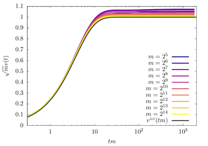
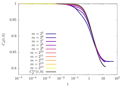
Figure 14: SymmDMFT predictions and large network scaling for lazy training in a single index model. Left: Projection $v(t)$ of the first layer weights onto the latent direction on timescales of the order $1/m$. The result for $m\to\infty$, ${v}^{\mbox{\tiny\rm lz1}}$, has been obtained by integrating analytically Eq. (E.55). Right: The behavior of $C_{d}(t,0)$ on timescales $t=\Theta(1)$, compared with the scaling theory for $m\to\infty$, namely ${C}^{\mbox{\tiny\rm lz2}}_{d}$. In both cases with $h(z)=\hat{\varphi}(z)=(9/10)z+z^{2}/2$, $\tau=0.3$ and $\alpha=0.3$, $\gamma_{0}=1$.

E.2.2 Second dynamical regime: $t=\Theta(1)$

We next consider $t=\Theta(1)$. One can show that the SymmDMFT equations are solved, up to higher order terms as $m\to\infty$, by the following ansatz

$$C_{d}(t,s) ={C}^{\mbox{\tiny\rm lz2}}_{d}(t,s)+o_{m}(1)\,,\;\;\;\;\;\;\;\;\;\;\;\;\;R_{d}(t,s)={R}^{\mbox{\tiny\rm lz2}}_{d}(t,s)+o_{m}(1)\,,$$

$$C_{o}(t,s) =\frac{1}{m}{C}^{\mbox{\tiny\rm lz2}}_{o}(t,s)+o_{m}(m^{-1})\,,\;\;\;\;\;\;R_{o}(t,s)=\frac{1}{m}{R}^{\mbox{\tiny\rm lz2}}_{o}(t,s)+o_{m}(m^{-1})\,,$$ (E.61)

$${\boldsymbol{v}}(t) =\frac{1}{\sqrt{m}}{{\boldsymbol{v}}}^{\mbox{\tiny\rm lz1}}_{\infty}+o_{m}(m^{-1/2})\,,\;\;\;\;\;\;\;\nu(t)={\nu}^{\mbox{\tiny\rm lz2}}(t)+o_{m}(1)\,,$$

with $\gamma(t)=\gamma_{0}+o_{m}(1)$ and

$${C}^{\mbox{\tiny\rm lz2}}_{o}(t,s)=-{C}^{\mbox{\tiny\rm lz2}}_{d}(t,s)+\|{{\boldsymbol{v}}}^{\mbox{\tiny\rm lz2}}_{\infty}\|^{2}\,,\;\;\;\;{R}^{\mbox{\tiny\rm lz2}}_{o}(t,s)=-{R}^{\mbox{\tiny\rm lz2}}_{d}(t,s)\,.$$ (E.62)

In other words, on this time scale first layer weights move by order one $\|{\boldsymbol{w}}_{i}(t)-{\boldsymbol{w}}_{i}(0)\|=\Theta(1)$, but in a linear subspace that is orthogonal to the latent space. Second layer weights do not move appreciably. As a consequence, no additional learning takes place in this regime, but the model begins to overfit the data.

Note that the above scaling form is compatible with the long time limit of the previous dynamical regime.

In order to define the equations for the functions on the right-hand side of Eq. (E.61) we define ${R}^{\mbox{\tiny\rm lz2}}_{A}$ and ${C}^{\mbox{\tiny\rm lz2}}_{A}$ to be the solution of

$$\begin{split}\delta(t-t^{\prime})&=\int_{t^{\prime}}^{t}\left[\delta(t-s)+{\Sigma}^{\mbox{\tiny\rm lz2}}_{R}(t,s)\right]{R}^{\mbox{\tiny\rm lz2}}_{A}(s,t^{\prime})\,{\rm d}s\,,\\ 0&=\int_{0}^{t}\left[\delta(t-s)+{\Sigma}^{\mbox{\tiny\rm lz2}}_{R}(t,s)\right]{C}^{\mbox{\tiny\rm lz2}}_{A}(s,t^{\prime})\,{\rm d}s+\int_{0}^{t^{\prime}}{\Sigma}^{\mbox{\tiny\rm lz2}}_{C}(t,s){R}^{\mbox{\tiny\rm lz2}}_{A}(t^{\prime},s)\,{\rm d}s\,,\end{split}$$ (E.63)

where

$$\begin{split}{\Sigma}^{\mbox{\tiny\rm lz2}}_{R}(t,s)&=\gamma_{0}^{2}\left(h^{\prime}({C}^{\mbox{\tiny\rm lz2}}_{d}(t,s))-h^{\prime}(0)\right){R}^{\mbox{\tiny\rm lz2}}_{d}(t,s)\,,\\ {\Sigma}^{\mbox{\tiny\rm lz2}}_{C}(t,s)&=\tau^{2}+\|\varphi\|^{2}-2\gamma_{0}\langle\nabla\hat{\varphi}(\boldsymbol{0}),{{\boldsymbol{v}}}^{\mbox{\tiny\rm lz1}}_{\infty}\rangle+\gamma_{0}^{2}\left(h({C}^{\mbox{\tiny\rm lz2}}_{d}(t,s))+h^{\prime}(0){C}^{\mbox{\tiny\rm lz2}}_{o}(t,s)\right)\,.\end{split}$$ (E.64)

Define the following memory kernels

$$\begin{split}{M}^{\mbox{\tiny\rm lz2}}_{R,d}(t,s)&=\alpha\gamma_{0}^{2}\left[{R}^{\mbox{\tiny\rm lz2}}_{A}(t,s)h^{\prime}({C}^{\mbox{\tiny\rm lz2}}_{d}(t,s))+{C}^{\mbox{\tiny\rm lz2}}_{A}(t,s)h^{\prime\prime}({C}^{\mbox{\tiny\rm lz2}}_{d}(t,s)){R}^{\mbox{\tiny\rm lz2}}_{d}(t,s)\right]\,,\\ {M}^{\mbox{\tiny\rm lz2}}_{R,o}(t,s)&=\alpha\gamma_{0}^{2}h^{\prime}(0){R}^{\mbox{\tiny\rm lz2}}_{A}(t,s)\,,\\ {M}^{\mbox{\tiny\rm lz2}}_{C,d}(t,s)&=\alpha\gamma_{0}^{2}h^{\prime}({C}^{\mbox{\tiny\rm lz2}}_{d}(t,s)){C}^{\mbox{\tiny\rm lz2}}_{A}(t,s)\,,\\ {M}^{\mbox{\tiny\rm lz2}}_{C,o}(t,s)&=\alpha\gamma_{0}^{2}h^{\prime}(0){C}^{\mbox{\tiny\rm lz2}}_{A}(t,s)\>.\end{split}$$ (E.65)

Substituting the ansatz (E.61) into the SymmDMFT equations, and using Eqs. (E.62), we obtain the following equations for ${C}^{\mbox{\tiny\rm lz2}}_{d}(t,t^{\prime})$, ${R}^{\mbox{\tiny\rm lz2}}_{d}(t,t^{\prime})$, ${\nu}^{\mbox{\tiny\rm lz2}}(t)$

$$\partial_{t}{C}^{\mbox{\tiny\rm lz2}}_{d}(t,t^{\prime}) =-{\nu}^{\mbox{\tiny\rm lz2}}(t){C}^{\mbox{\tiny\rm lz2}}_{d}(t,t^{\prime})+{\alpha}\gamma_{0}\langle\nabla\hat{\varphi}^{\prime}(\boldsymbol{0}),{{\boldsymbol{v}}}^{\mbox{\tiny\rm lz1}}_{\infty}\rangle\int_{0}^{t}{R}^{\mbox{\tiny\rm lz2}}_{A}(t,s){\rm d}s$$

$$\;\;\;-\int_{0}^{t}{\rm d}s\left[{M}^{\mbox{\tiny\rm lz2}}_{R,d}(t,s){C}^{\mbox{\tiny\rm lz2}}_{d}(t^{\prime},s)+{M}^{\mbox{\tiny\rm lz2}}_{R,o}(t,s){C}^{\mbox{\tiny\rm lz2}}_{o}(t^{\prime},s)\right]\,{\rm d}s$$ (E.66)

$$\;\;\;-\int_{0}^{t^{\prime}}\left[{M}^{\mbox{\tiny\rm lz2}}_{C,d}(t,s){R}^{\mbox{\tiny\rm lz2}}_{d}(t^{\prime},s)+{M}^{\mbox{\tiny\rm lz2}}_{C,o}(t,s){R}^{\mbox{\tiny\rm lz2}}_{o}(t^{\prime},s)\right]{\rm d}s\,,$$

$$\partial_{t}{R}^{\mbox{\tiny\rm lz2}}_{d}(t,t^{\prime}) =-{\nu}^{\mbox{\tiny\rm lz2}}(t){R}^{\mbox{\tiny\rm lz2}}_{d}(t,t^{\prime})+\delta(t-t^{\prime})$$ (E.67)

$$\;\;\;-\int_{t^{\prime}}^{t}\left[{M}^{\mbox{\tiny\rm lz2}}_{R,d}(t,s){R}^{\mbox{\tiny\rm lz2}}_{d}(s,t^{\prime})+{M}^{\mbox{\tiny\rm lz2}}_{R,o}(t,s){R}^{\mbox{\tiny\rm lz2}}_{o}(s,t^{\prime})\right]{\rm d}s\,,$$

$${\nu}^{\mbox{\tiny\rm lz2}}(t) =\alpha\gamma_{0}\langle\nabla\hat{\varphi}^{\prime}(\boldsymbol{0}),{{\boldsymbol{v}}}^{\mbox{\tiny\rm lz1}}_{\infty}\rangle\int_{0}^{t}{R}^{\mbox{\tiny\rm lz2}}_{A}(t,s)\,{\rm d}s-\int_{0}^{t}\left[{M}^{\mbox{\tiny\rm lz2}}_{R,d}(t,s){C}^{\mbox{\tiny\rm lz2}}_{d}(t,s)+{M}^{\mbox{\tiny\rm lz2}}_{R,o}(t,s){C}^{\mbox{\tiny\rm lz2}}_{o}(t,s)\right]\,{\rm d}s$$

$$\;\;\;-\int_{0}^{t}\left[{M}^{\mbox{\tiny\rm lz2}}_{C,d}(t,s){R}^{\mbox{\tiny\rm lz2}}_{d}(t,s)+{M}^{\mbox{\tiny\rm lz2}}_{C,o}(t,s){R}^{\mbox{\tiny\rm lz2}}_{o}(t,s)\right]\,{\rm d}s\,.$$ (E.68)

Finally, the train and test errors converge to well defined limits for $t$ fixed and $m\to\infty$:

$$e_{\mbox{{\rm\footnotesize tr}}}(t,\gamma_{0})={e}^{\mbox{\tiny\rm lz2}}_{\mbox{{\rm\footnotesize tr}}}(t,\gamma_{0})+o_{m}(1)\,,\;\;\;\;\;e_{\mbox{\rm\footnotesize ts}}(t,\gamma_{0})={e}^{\mbox{\tiny\rm lz2}}_{\mbox{\rm\footnotesize ts}}(t,\gamma_{0})+o_{m}(1)\,.,$$ (E.69)

where

$${e}^{\mbox{\tiny\rm lz2}}_{\mbox{{\rm\footnotesize tr}}}(t,\gamma_{0})=-\frac{1}{2}{C}^{\mbox{\tiny\rm lz2}}_{A}(t,t)\,,\;\;\;{e}^{\mbox{\tiny\rm lz2}}_{\mbox{\rm\footnotesize ts}}(t,\gamma_{0})=\frac{1}{2}{\Sigma}^{\mbox{\tiny\rm lz2}}_{C}(t,t)\,.$$ (E.70)

Note that, using Eqs. (E.62), (E.64), and the fact that ${C}^{\mbox{\tiny\rm lz2}}_{d}(t,t)=1$ (because of the unit norm constraint on the first layer weights), we get

$${e}^{\mbox{\tiny\rm lz2}}_{\mbox{\rm\footnotesize ts}}(t,\gamma_{0})=\frac{1}{2}\Big{\{}\tau^{2}+\|\varphi\|^{2}-2\gamma_{0}\langle\nabla\hat{\varphi}(\boldsymbol{0}),{{\boldsymbol{v}}}^{\mbox{\tiny\rm lz1}}_{\infty}\rangle+\gamma_{0}^{2}\big{(}h(1)-h^{\prime}(0)+h^{\prime}(0)\|{{\boldsymbol{v}}}^{\mbox{\tiny\rm lz1}}_{\infty}\|^{2}\big{)}\Big{\}}\,.$$ (E.71)

Using Eq. (E.57), we obtain that the asymptotic test error in this dynamical regime is constant and equal to the test error achieved at the end of the previous regime, namely ${e}^{\mbox{\tiny\rm lz2}}_{\mbox{\rm\footnotesize ts}}(t,\gamma_{0})={e}^{\mbox{\tiny\rm lz1}}_{\mbox{\rm\footnotesize ts},\infty}$, cf. Eq. (E.59). As anticipated, no learning takes place on this timescale.

The predictions of Eqs. (E.61) are tested in the right panel of Fig. 14. We plot the correlation function $C_{d}(t,0)$ for several values of $m$, as obtained by solving the SymmDMFT equations. We compare these results with the $m\to\infty$ prediction ${C}^{\mbox{\tiny\rm lz2}}_{d}(t,0)$ obtained by solving Eqs. (E.66) to (E.68). We observe collapse of finite $m$ curves on the large $m$ asymptotics supporting our conclusions.

In Fig. 15 we plot the behavior of the train and test error both on timescales $t=\Theta(1/m)$ (left frame, plotting $e_{\mbox{{\rm\footnotesize tr}}}(t,\gamma_{0})$, $e_{\mbox{\rm\footnotesize ts}}(t,\gamma_{0})$ versus $tm$) and $t=\Theta(1)$ (right frame, plotting $e_{\mbox{{\rm\footnotesize tr}}}(t,\gamma_{0})$, $e_{\mbox{\rm\footnotesize ts}}(t,\gamma_{0})$ versus $tm$). We the solutions of SymmDMFT equations at increasing values of $m$ with the theory scaling theory presented in the previous section (for $t=\Theta(1/m)$, left frame) and in this section (for $t=\Theta(1)$, right frame). As anticipated, we observe the following:

• On the time scale $t=\Theta(1/m)$ (left panel), test and train error collapse (as $m\to\infty$) on a common limiting curve ${e}^{\mbox{\tiny\rm lz1}}_{\mbox{{\rm\footnotesize tr}}}(\hat{t},\gamma_{0})={e}^{\mbox{\tiny\rm lz1}}_{\mbox{\rm\footnotesize ts}}(\hat{t},\gamma_{0})$ which converges, for large $\hat{t}$, to the positive limiting value ${e}^{\mbox{\tiny\rm lz1}}_{\mbox{\rm\footnotesize ts},\infty}$ characterized in the previous section.

• On the time scale $t=\Theta(1)$ (right panel), test and train error collapse (as $m\to\infty$) on two distinct limiting curves. The first one is constant and equal to ${e}^{\mbox{\tiny\rm lz1}}_{\mbox{\rm\footnotesize ts},\infty}$. The second one decreases from ${e}^{\mbox{\tiny\rm lz1}}_{\mbox{\rm\footnotesize ts},\infty}$ to $0$ and is predicted by the asymptotic theory in this section, cf. Eq. (E.70).

Note that, in the example of Fig. 15, the initialization $\gamma_{0}$ is sufficiently large that the train error decreases to zero on the time scale $\Theta(1)$, namely $\gamma_{0}>\gamma^{*}_{\mbox{\tiny\rm GF}}(\alpha,\varphi,\tau)$, for a suitable threshold $\gamma^{*}_{\mbox{\tiny\rm GF}}(\alpha,\varphi,\tau)$. As we will see in the next section, a third dynamical regime emerges when $\gamma_{0}<\gamma^{*}_{\mbox{\tiny\rm GF}}(\alpha,\varphi,\tau)$.

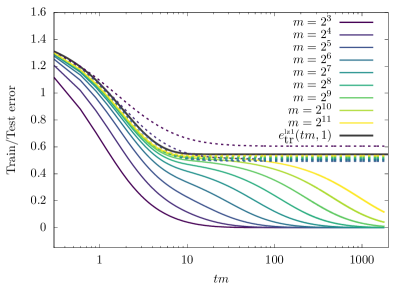
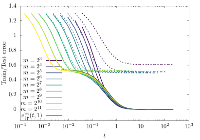
Figure 15: SymmDMFT predictions and large network scaling for lazy training in a single index model: train and test error. Left frame: train and test error on the time scale $t=\Theta(1/m)$ for several values of $m$, together with the asymptotic prediction as $m\to\infty$ on this time scale ${e}^{\mbox{\tiny\rm lz1}}_{\mbox{{\rm\footnotesize tr}}}(\hat{t},\gamma_{0})={e}^{\mbox{\tiny\rm lz1}}_{\mbox{\rm\footnotesize ts}}(\hat{t},\gamma_{0})$. Right: train and test error on the time scale $t=\Theta(1)$ for several values of $m$, together with the asymptotic prediction as $m\to\infty$ on this time scale ${e}^{\mbox{\tiny\rm lz2}}_{\mbox{{\rm\footnotesize tr}}}(t,\gamma_{0})$. Here $\gamma_{0}=1$, $h(z)=\hat{\varphi}(z)=(9/10)z+z^{2}/2$, $\tau=0.3$, $\alpha=0.3$.

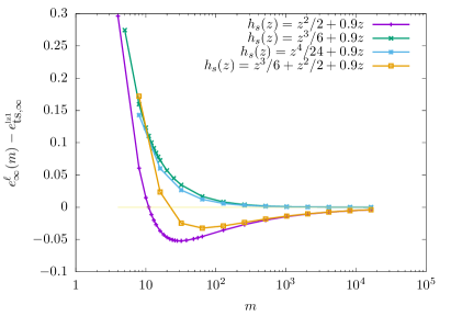
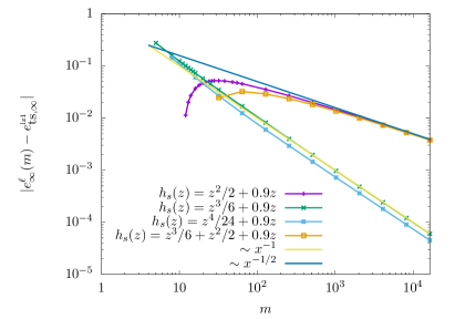
Figure 16: The asymptotic behavior of the test error as a function of $m$ for different $h(z)=\hat{\varphi}(z)$. We observe that soon as $h(z)$ contains a $z^{2}$ term, the NTK limit for $m\to\infty$ is approached from below (left panel). Furthermore the speed of the convergence to the limiting value depends crucially on whether a $z^{2}$ monomial is present in the Taylor expansion of $h(z)$ (right panel). The data has been produced with $\alpha=0.3$ and $\tau=0.6$.

E.2.3 The algorithmic interpolation threshold

The asymptotic theory within the second dynamical regime, described in Section E.2.2, turns out to be equivalent to the one in the pure-noise model, Section E.1.2, up to a change of variables. Namely, defining

$$\tilde{C}_{o}(t,s)={C}^{\mbox{\tiny\rm lz2}}_{o}(t,s)+\|{{\boldsymbol{v}}}^{\mbox{\tiny\rm lz1}}_{\infty}\|^{2}\,,$$ (E.72)

with initial condition $\tilde{C}_{o}(0,0)=-1$ , reduce the equations of Section E.2.2 to the ones of Section E.1.2 with noise level $\tau$ replaced by

$$\tau^{\prime 2}=\tau^{2}+\|\varphi\|^{2}-\frac{\|\nabla\hat{\varphi}(\boldsymbol{0})\|^{2}}{h^{\prime}(0)}\,.$$ (E.73)

The interpretation of this reduction is simple. On the time scale $t=\Theta(1)$, the first layer weights move orthogonally to the latent subspace spanned by ${\boldsymbol{U}}$. Hence, the dynamics on this timescale is not affected by the signal and only attempts to fit the labels noise. The noise is inflated as per Eq. (E.73), because the network is not able to fit beyond the linear part of the target distribution.

As a corollary of the above equivalence, the interpolation threshold of the $k$-index model coincides with with the interpolation threshold on pure noise data with noise level given by Eq. (E.73). Using the extended notation $\gamma^{*}_{\mbox{\tiny\rm GF}}(\alpha,\varphi,\tau)$ to indicate the dependence on the underlying data distribution (which is parametrized by $\varphi,\tau$), we can write the stated relation as

$$\gamma^{*}_{\mbox{\tiny\rm GF}}(\alpha,\varphi,\tau)=\Big{(}\tau^{2}+\|\varphi\|^{2}-\frac{\|\nabla\hat{\varphi}(\boldsymbol{0})\|^{2}}{h^{\prime}(0)}\Big{)}^{1/2}\gamma^{*}_{\mbox{\tiny\rm GF}}(\alpha,0,1)\,.$$ (E.74)

(Here we used the invariance under rescaling in the pure noise model, which implies $\gamma^{*}_{\mbox{\tiny\rm GF}}(\alpha,0,\tau^{2})=\tau\gamma^{*}_{\mbox{\tiny\rm GF}}(\alpha,0,1)$.)

E.2.4 Dependence on $m$

Within NTK theory, it is normally assumed that optimal models are achieved at very large network sizes $m\to\infty$. Empirical results contradicting this expectation have been put forward in [VBN22], but no theoretical analysis was provided either in [VBN22] or in subsequent work. We can use the SymmDMFT theory to fill this gap and study the dependence of test error on the number of neurons $m$ under lazy initialization. We choose $\gamma_{0}>\gamma^{*}_{\rm GF}(\alpha,\varphi,\tau)$, and therefore vanishing training error is reached during the second dynamical regime, i.e. for $t=\Theta(1)$: this is therefore the last dynamical regime. Throughout this regime, we have $\gamma(t)=\gamma_{0}+o_{m}(1)$.

Recalling that $e_{\mbox{\rm\footnotesize ts}}(t,\gamma_{0},m,\alpha)$ is the test error at time $t$ in this setting, as predicted by SymmDMFT we consider the limit

$$e^{\ell}_{\infty}(\gamma_{0},m,\alpha)=\lim_{t\to\infty}e_{\mbox{\rm\footnotesize ts}}(t,\gamma_{0},m,\alpha)\,.$$ (E.75)

We note that, for $\gamma_{0}>\gamma^{*}_{\rm GF}(\alpha,\varphi,\tau)$, we expect

$$\lim_{m\to\infty}e^{\ell}_{\infty}(\gamma_{0},m,\alpha)={e}^{\mbox{\tiny\rm lz1}}_{\mbox{\rm\footnotesize ts},\infty},$$ (E.76)

to be given by Eq. (E.59).

In Fig. 16 we plot the SymmDMFT prediction for $e^{\ell}_{\infty}(\gamma_{0},m,\alpha)$ as a function of $m$ for several choices of $h$ (we use $h=\hat{\varphi}$ here). The limit $m\to\infty$ of these curves matches ${e}^{\mbox{\tiny\rm lz1}}_{\mbox{\rm\footnotesize ts},\infty}$ as expected. However we empirically observe that $e^{\ell}_{\infty}(\gamma_{0},m,\alpha)$ approaches ${e}^{\mbox{\tiny\rm lz1}}_{\mbox{\rm\footnotesize ts},\infty}$ in two qualitatively different ways:

• In the cases we consider that have $h^{\prime\prime}(0)\neq 0$, ${e}^{\mbox{\tiny\rm lz1}}_{\mbox{\rm\footnotesize ts},\infty}$ is approached from below as $m\to\infty$, and $e^{\ell}_{\infty}(\gamma_{0},m,\alpha)$ is non-monotone. We also observe that, for the values of $m$ we consider, the approach to the asymptotic value is compatible with a rate $m^{-1/2}$: $e^{\ell}_{\infty}(\gamma_{0},m,\alpha)={e}^{\mbox{\tiny\rm lz1}}_{\mbox{\rm\footnotesize ts},\infty}-\Theta(m^{-1/2})$.

• In the cases we consider that have $h^{\prime\prime}(0)\neq 0$, then ${e}^{\mbox{\tiny\rm lz1}}_{\mbox{\rm\footnotesize ts},\infty}$ is approached from above as $m\to\infty$, and $e^{\ell}_{\infty}(\gamma_{0},m,\alpha)$ is typically monotone. In this case the approach to the limiting behavior is compatible with a rate $m^{-1}$: $e^{\ell}_{\infty}(\gamma_{0},m,\alpha)={e}^{\mbox{\tiny\rm lz1}}_{\mbox{\rm\footnotesize ts},\infty}+\Theta(m^{-1})$.

The first scenario is the generic one, and similar to what is observed in [VBN22] for actual neural networks. An intuitive explanation is that –at finite $m$– the projection of neurons onto the latent space $\|{{\boldsymbol{v}}}^{\mbox{\tiny\rm lz1}}_{\infty}\|=\Theta(1/\sqrt{m})$ is sufficient for the network to partially learn the quadratic component of the target function. In order to establish on more solid grounds these empirical observations one should study the $1/m$ corrections to the scaling theory developed here. This is left for future work.

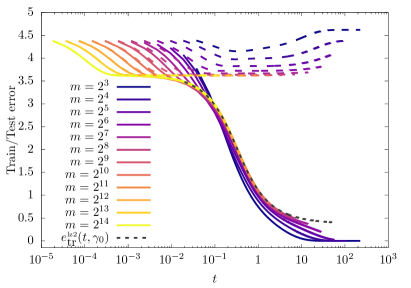
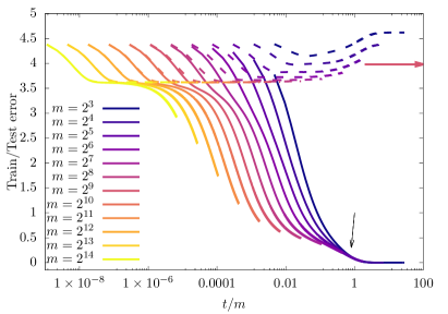
Figure 17: Train error (solid curves) and test error (dashed curves) for a model trained on a single index data with $h(z)=(9/10)z+z^{2}/2=\hat{\varphi}(z)$. The noise level is $\tau=2.5$ and initialization $a(0)=\gamma_{0}\sqrt{m}$, $\gamma_{0}<\gamma^{*}_{\mbox{\tiny\rm GF}}(\alpha,\varphi,\tau)$. Left panel: timescales of order one. The grey dashed line corresponds to the scaling solution for $m\to\infty$ when the second layer does not evolve with GF. Right panel: same data plotted versus $t/m$, to explore timescales of order $m$. The arrows show scaling appearing and curves collapsing on a master curve.

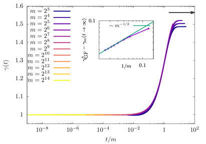
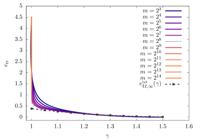
Figure 18: Training a two layer network in the same setting of Figure 17. Left panel: second layer weights on the timescale of order $m$. The black arrow corresponds to the interpolation threshold for a model, $\gamma_{GF}^{*}(\alpha,\tau)$ obtained by fitting the relaxation time as a function of the weights of an lazy initialized model for $\gamma_{0}>\gamma_{\rm GF}^{*}(\alpha,\tau)$. The second layer weights, at finite $m$ develop a plateau at long time. In the inset we show the approach of this plateaus to the limiting value given by $\gamma_{\mbox{\tiny\rm GF}}^{*}(\alpha,\varphi,\tau)$. Right panel: parametric plot of the train error as a function of the scaled weights of the second layer. The dashed gray dashed line corresponds to the extrapolated train error for an network with second layer weights fixed to the corresponding value in the $m\to\infty$ (as extracted from the numerical integration of the scaling theory).

E.2.5 Third dynamical regime: $t=\Theta(m)$

As for the pure noise case, beyond the time scale $t=\Theta(1)$, we distinguish two situations. If $\gamma_{0}>\gamma^{*}_{\mbox{\tiny\rm GF}}(\alpha,\varphi,\tau)$, then vanishing training error is reached within the second dynamical regime $t=\Theta(1)$. If $\gamma_{0}<\gamma_{\rm GF}^{*}(\alpha,\varphi,\tau)$, GF dynamics develops an additional regime for $t=\Theta(m)$. In this section, we study this third regime.

In Figure 17, we plot the SymmDMFT predictions for train and test errors as a function of time for several values of $m$, for a setting with $\gamma_{0}<\gamma_{\rm GF}^{*}(\alpha,\varphi,\tau)$. In particular, in Fig.17-left we plot train and test error as a function of $t$. The curves for the train error for increasing value of $m$ collapse on limit curve given by ${e}^{\mbox{\tiny\rm lz2}}_{\mbox{{\rm\footnotesize tr}}}(t,\gamma_{0})$ characterized in Section E.2.2. In other words, the dynamics on this timescales follows the scaling theory of Section E.2.2. However in this case $\gamma_{0}<\gamma_{\rm GF}^{*}(\alpha,\varphi,\tau)$, whence by definition ${e}^{\mbox{\tiny\rm lz2}}_{\mbox{{\rm\footnotesize tr}},\infty}>0$. This correspond to the limit curve in Fig. 17-left having a strictly positive asymptote.

Figure 17-right shows train and test error plotted against $t/m$. We observe that curves training error curves collapse on a common limit, that decreases from ${e}^{\mbox{\tiny\rm lz2}}_{\mbox{{\rm\footnotesize tr}},\infty}$ to $0$, while test error curves increase above the plateau ${e}^{\mbox{\tiny\rm lz1}}_{\mbox{\rm\footnotesize ts},\infty}$. This suggests the following limit behavior

$$\begin{split}\lim_{m\to\infty}e_{\mbox{{\rm\footnotesize tr}}}(m\hat{t},\gamma_{0},m)&={e}^{\mbox{\tiny\rm lz3}}_{\mbox{{\rm\footnotesize tr}}}(\hat{t},\gamma_{0})\\ \lim_{m\to\infty}e_{\mbox{\rm\footnotesize ts}}(m\hat{t},\gamma_{0},m)&={e}^{\mbox{\tiny\rm lz3}}_{\mbox{\rm\footnotesize ts}}(\hat{t},\gamma_{0})\>.\end{split}$$ (E.77)

In order to further explore the GF dynamics in this regime, in Fig. 18-left we plot the evolution of the second layer rescaled weights against $t/m$. The curves for increasing values of $m$ collapse on a master curve, suggesting the existence of a limit

$$\lim_{m\to\infty}\gamma(m\hat{t},\gamma_{0})={\gamma}^{\mbox{\tiny\rm lz3}}(\hat{t},\gamma_{0})\>.$$ (E.78)

The limit curve ${\gamma}^{\mbox{\tiny\rm lz3}}(\hat{t},\gamma_{0})$ increases from $\gamma_{0}$ to a limit value:

$$\lim_{\hat{t}\to\infty}{\gamma}^{\mbox{\tiny\rm lz3}}(\hat{t},\gamma_{0})={\gamma}^{\mbox{\tiny\rm lz3}}_{\infty}(\gamma_{0}).$$ (E.79)

As in Section E.2.5 we consider the inverse function of $t\mapsto{\gamma}^{\mbox{\tiny\rm lz3}}(t,\gamma_{0})$, denoted by $\gamma\mapsto\tilde{\gamma}^{-1}(\gamma,\gamma_{0})$. In Fig. 18-right we plot the train error as a function of the second layer weights $\gamma(t)$. Again, for increasing values of $m$ the curves collapse on a master curve which is given by

$$\varepsilon(\gamma,\gamma_{0})={e}^{\mbox{\tiny\rm lz3}}_{\mbox{{\rm\footnotesize tr}}}(\tilde{\gamma}^{-1}(\gamma,\gamma_{0}),\gamma_{0})$$ (E.80)

We then also plot in Fig.18-right the asymptotic value of the train error for a network initialized with second layer weights blocked at an initialization scale $\gamma$, call it ${e}^{\mbox{\tiny\rm lz2}}_{\mbox{{\rm\footnotesize tr}},\infty}(\gamma)$.

The curves $\varepsilon(\gamma,\gamma_{0})$ appear to have a vertical segment (corresponding to $t=o(m)$) in which the training error decreases, while $\gamma(t)=\gamma_{0}+o_{m}(1)$ is nearly unchanged, and a continuously decreasing segment in which $\gamma(t)$ increases while $e_{\mbox{{\rm\footnotesize tr}}}(t,\gamma_{0})$ decreases to $0$ (corresponding to $t=\Theta(m)$). In the second phase, the curves appear to converge to ${e}^{\mbox{\tiny\rm lz2}}_{\mbox{{\rm\footnotesize tr}},\infty}(\gamma)$ as $m\to\infty$. This suggests

$$\varepsilon(\gamma,\gamma_{0})={e}^{\mbox{\tiny\rm lz2}}_{\mbox{{\rm\footnotesize tr}},\infty}(\gamma)\ \ \ \ \forall\gamma\geq\gamma_{0}\>.$$ (E.81)

In other words the dynamics on timescales of order $m$ is adiabatic also in the multi index case. For a small change of the second layer weights on a scale of order $\sqrt{m}$, the train error relaxes to its asymptotic value on timescales of order one. This graph suggests that the limit value of $\gamma(t)$ coincides with the critical value for interpolation. Namely recalling the definition (E.79) for the asymptotic value of $\gamma(t)$, we have

$${\gamma}^{\mbox{\tiny\rm lz3}}_{\infty}(\gamma_{0})=\gamma_{\rm GF}^{*}(\alpha,\varphi,\tau)$$ (E.82)

where the interpolation threshold in the multi-index model $\gamma_{\rm GF}^{*}(\alpha,\varphi,\tau)$ is related to the interpolation threshold in the pure noise model via Eq. (E.74).

Appendix F Dynamical regimes: Mean field initialization

In this section we assume the initialization of the weights of the second layer is kept of order one. To be definite, we set $a(0)=a_{0}$, independent of $m$. This corresponds to the mean field initialization studied in [MMN18, CB18, RVE22].

Specializing to the data distribution considered here, earlier work characterized the dynamics up to time $T$, under a few settings (which prove equivalent in this regime):

• One-pass SGD, with stepsize ${\varepsilon}\ll 1/d$ and therefore time horizons such that $T\ll d/n$ (the latter inequality follows from $T\leq n{\varepsilon}$ for one-pass SGD). In this case, the dynamics is characterized by a set of ODEs for for the projections of the weights on the latent space and inner products between weights.

• Gradient flow in the population risk, which admits the same characterization and corresponds to the limit $n\to\infty$ of the above.

• The limit of the above regimes for large width $m\to\infty$. This is characterized by a partial differential equation for the distribution of projections of first layer weights onto the latent space, provided $T\leq c_{0}\log m$, for $c_{0}$ a sufficiently small constant.

We refer to [BES⁺22, DLS22, AAM22, BEG⁺22, ASKL23, BMZ24] for a few pointers to this literature. In all of these settings, the train error remains close to the test error. In contrast, the analysis presented here allow us to explore the overfitting regime.

Section F.1, we will focus on a pure noise data distribution, while Section F.2, considers a multi-index model. As in the case of lazy initializations, we consider first the limit $n,d\to\infty$ at $n/md=\alpha$ and $m$ fixed (hence characterized by SymmDMFT ) and subsequently study dynamical regimes emerging as $m\to\infty$ at $n/md=\alpha$ fixed.

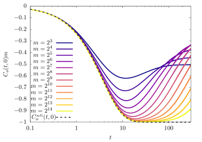
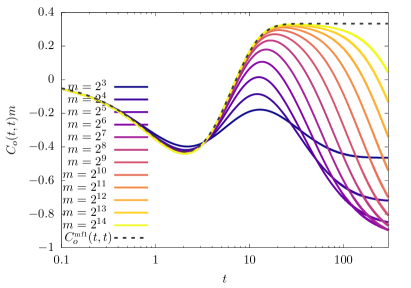
Figure 19: Training on pure noise data under mean-field initialization: $t=\Theta(1)$ regime. We plot $C_{o}(t,0)$ and $C_{o}(t,t)$ as given by solving the SymmDMFT equations for different values of $m$ and compare them with the asymptotic solution of Section F.1.1. Here we use $\tau=0.6$, $\alpha=0.3$ and $h(z)=(9/10)z+z^{3}/6$. Note that the vertical axis is multiplied by a factor $m$, in agreement with the prediction of Eq. (F.2).

F.1 Pure noise model

Under the pure noise model, we have $\varphi=\hat{\varphi}=0$. We identify three distinct dynamical regimes:

• $t=O(1)$: $a(t)=a_{0}+o_{m}(1)$, $e_{\mbox{{\rm\footnotesize tr}}}(t)=\tau^{2}/2+o_{m}(1)$, and $\|{\boldsymbol{w}}_{i}(t)-{\boldsymbol{w}}_{i}(0)\|=o_{m}(1)$. In words, the weights change minimally and the train error remains close to the one of the null network $f({\boldsymbol{x}};{\boldsymbol{\theta}})\approx 0$ (Section F.1.1).

• $t=\Theta(\sqrt{m})$: $a(t)=\Theta(1)$, $e_{\mbox{{\rm\footnotesize tr}}}(t)=\tau^{2}/2+o_{m}(1)$, and $\|{\boldsymbol{w}}_{i}(t)-{\boldsymbol{w}}_{i}(0)\|=\Theta(1)$. Namely, weights change but the train error does not change significantly. (Section F.1.2).

• $t=\Theta(m)$. In this regime $a(t)=\sqrt{m}\gamma(t/m)+o_{m}(1)$, and therefore the network complexity becomes large enough for it to fit the noise. The dynamics on this timescale is closely related to the one under lazy initialization, studied in Section E.1.4. In particular, $\gamma(\hat{t})$ converge to the interpolation threshold $\gamma^{*}_{\mbox{\tiny\rm GF}}(\alpha,\tau)$ if $\hat{t}\to\infty$ (after $m\to\infty$). (Section F.1.3).

F.1.1 First dynamical regime: $t=O(1)$

In this dynamical regime, the SymmDMFT equations are solved by the following scaling ansatz

$$C_{d}(t,s) =1+o_{m}(1) R_{d}(t,s) =\vartheta(t-s)+o_{m}(1)\,,$$ (F.1)

$$mC_{o}(t,s) ={C}^{\mbox{\tiny\rm mf1}}_{o}(t,s)+o_{m}(1) mR_{o}(t,s) ={R}^{\mbox{\tiny\rm mf1}}_{o}(t,s)+o_{m}(1)\,,$$ (F.2)

$$a(t) =a_{0}+o_{m}(1) \nu(t) =o_{m}(1)\,.$$ (F.3)

Furthermore we have

$${R}^{\mbox{\tiny\rm mf1}}_{A}(t,s)=\delta(t-s)+o_{m}(1)\ \ \ \ {C}^{\mbox{\tiny\rm mf1}}_{A}(t,s)=-\tau^{2}+o_{m}(1)\,,$$ (F.4)

Plugging the scaling ansatz in the SymmDMFT , we obtain equations determining the scaling functions ${C}^{\mbox{\tiny\rm mf1}}_{o}$, ${R}^{\mbox{\tiny\rm mf1}}_{o}$. Defining

$$\rho_{0}:=\alpha a^{2}_{0}h^{\prime}(0)$$ (F.5)

we have

$$\begin{split}{R}^{\mbox{\tiny\rm mf1}}_{o}(t,s)&=\left[e^{-\rho_{0}(t-s)}-1\right]\vartheta(t-s)\,,\\ {C}^{\mbox{\tiny\rm mf1}}_{o}(t,t^{\prime})&=\left[\left[\frac{2\tau^{2}}{\rho_{0}}-\frac{1}{\rho_{0}}\left(\tau^{2}-\rho_{0}\right)\right]e^{-2\rho_{0}t^{\prime}}-\frac{\tau^{2}}{\rho_{0}}e^{-\rho_{0}t^{\prime}}\right]e^{-\rho_{0}(t-t^{\prime})}\\ &+\frac{\tau^{2}-\rho_{0}}{\rho_{0}}-\frac{\tau^{2}}{\rho_{0}}e^{-\rho_{0}t^{\prime}}\,.\end{split}$$ (F.6)

In particular

$$\begin{split}\lim_{t\to\infty}{C}^{\mbox{\tiny\rm mf1}}_{o}(t,t)&=\frac{\tau^{2}-\rho_{0}}{\rho_{0}}\,,\\ \lim_{t\to\infty}{C}^{\mbox{\tiny\rm mf1}}_{o}(t,t^{\prime})&=\frac{\tau^{2}-\rho_{0}}{\rho_{0}}-\frac{\tau^{2}}{\rho_{0}}e^{-\rho_{0}t^{\prime}}\,,\\ \lim_{t\to\infty,t^{\prime}\to\infty,t-t^{\prime}\geq 0}{C}^{\mbox{\tiny\rm mf1}}_{o}(t,t^{\prime})&=\frac{\tau^{2}-\rho_{0}}{\rho_{0}}\,.\end{split}$$ (F.7)

The equations (F.4) imply that the train error is constant in this regime and equal to

$$e_{\mbox{{\rm\footnotesize tr}}}(t)=\frac{\tau^{2}}{2}+o_{m}(1)\,.$$ (F.8)

In other words, in this regime both first and second layer weights change minimally and the resulting error remains close to the one to the null function $f({\boldsymbol{x}};{\boldsymbol{\theta}})\approx 0$. We will see that this regime is significantly more interesting for the case of data with a signal, see Section F.2. We note in passing that the limit value $\langle{\boldsymbol{w}}_{j},{\boldsymbol{w}}_{j}\rangle\approx\frac{\tau^{2}-\rho_{0}}{m\rho_{0}}$ for $i\neq j$ corresponds to minimizing the empirical risk under the linear approximation in which $\sigma(z)$ is replaced by $\sqrt{h^{\prime}(0)}z$.

The above predictions are tested in Fig. 19 where we plot $C_{o}(t,t)$ and $C_{o}(t,0)$ for different values of $m$ and check their approach to the scaling functions ${C}^{\mbox{\tiny\rm mf1}}_{o}(t,0)$ and ${C}^{\mbox{\tiny\rm mf1}}_{o}(t,t)$.

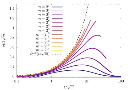
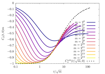
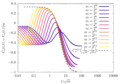
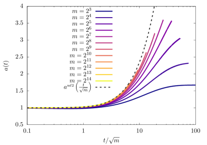
Figure 20: Training on pure noise data under mean-field initialization: $t=\Theta(1)$ regime, under the same setting as in Fig. 19. We plot the solutions of the SymmDMFT equations for several values of $m$ as a function of $t/\sqrt{m}$. We compare these to the $m\to\infty$ scaling theory of Section F.1.2, i.e. to numerical solutions of Eqs. (F.14) to (F.17).

F.1.2 Second dynamical regime: $t=\Theta(\sqrt{m})$

We now consider the case in which time scales as $\sqrt{m}$. The following asymptotic forms can be checked to solve the SymmDMFT equations, up to higher order terms, for suitable choices of the scaling functions on the right-hand side:

$$C_{d}(t\sqrt{m},s\sqrt{m}) ={C}^{\mbox{\tiny\rm mf2}}_{d}(t,s)+o_{m}(1) R_{d}(t\sqrt{m},s\sqrt{m}) ={R}^{\mbox{\tiny\rm mf2}}_{d}(t,s)+o_{m}(1)\,,$$ (F.9)

$$C_{o}(t\sqrt{m},s\sqrt{m}) =\frac{1}{m}{C}^{\mbox{\tiny\rm mf2}}_{o}(t,s)+o_{m}(m^{-1}) R_{o}(t\sqrt{m},s\sqrt{m}) =\frac{1}{m}{R}^{\mbox{\tiny\rm mf2}}_{o}(t,s)+o_{m}(m^{-1})\,,$$ (F.10)

$$\sqrt{m}R_{A}(t\sqrt{m},s\sqrt{m}) =\delta(t-s)+o_{m}(1) C_{A}(t\sqrt{m},s\sqrt{m}) =-\tau^{2}+o_{m}(1)\,,$$ (F.11)

$$\sqrt{m}\nu(t\sqrt{m}) ={\nu}^{\mbox{\tiny\rm mf2}}(t)+o_{m}(1) a(t\sqrt{m}) ={a}^{\mbox{\tiny\rm mf2}}(t)+o_{m}(1)\,.$$ (F.12)

Plugging this scaling ansatz into the SymmDMFT equations we get the constraints

$$\begin{split}{R}^{\mbox{\tiny\rm mf2}}_{o}(t,s)&=-{R}^{\mbox{\tiny\rm mf2}}_{d}(t,s)\,,\\ {C}^{\mbox{\tiny\rm mf2}}_{o}(t,s)&=-{C}^{\mbox{\tiny\rm mf2}}_{d}(t,s)+\frac{\tau^{2}}{\alpha h^{\prime}(0)({a}^{\mbox{\tiny\rm mf2}}(t))^{2}}\,.\end{split}$$ (F.13)

We also obtain that the following equations must be satisfied by ${C}^{\mbox{\tiny\rm mf2}}_{d}(t,t^{\prime})$, ${R}^{\mbox{\tiny\rm mf2}}_{d}(t,t^{\prime})$, ${a}^{\mbox{\tiny\rm mf2}}(t)$, ${\nu}^{\mbox{\tiny\rm mf2}}(t)$,

$$\partial_{t}{C}^{\mbox{\tiny\rm mf2}}_{d}(t,t^{\prime}) =-{\nu}^{\mbox{\tiny\rm mf2}}(t){C}^{\mbox{\tiny\rm mf2}}_{d}(t,t^{\prime})+\alpha\tau^{2}{a}^{\mbox{\tiny\rm mf2}}(t)\int_{0}^{t}{a}^{\mbox{\tiny\rm mf2}}(s)h^{\prime\prime}({C}^{\mbox{\tiny\rm mf2}}_{d}(t,s)){R}^{\mbox{\tiny\rm mf2}}_{d}(t,s){C}^{\mbox{\tiny\rm mf2}}_{d}(t^{\prime},s)\,{\rm d}s$$ (F.14)

$$+\alpha\tau^{2}{a}^{\mbox{\tiny\rm mf2}}(t)\int_{0}^{t^{\prime}}{a}^{\mbox{\tiny\rm mf2}}(s)\left[h^{\prime}({C}^{\mbox{\tiny\rm mf2}}_{d}(t,s))-h^{\prime}(0)\right]{R}^{\mbox{\tiny\rm mf2}}_{d}(t^{\prime},s)\,{\rm d}s\,,$$

$$\partial_{t}{R}^{\mbox{\tiny\rm mf2}}_{d}(t,t^{\prime}) =\delta(t-t^{\prime})-{\nu}^{\mbox{\tiny\rm mf2}}(t){R}^{\mbox{\tiny\rm mf2}}_{d}(t,t^{\prime})$$ (F.15)

$$+\alpha\tau^{2}{a}^{\mbox{\tiny\rm mf2}}(t)\int_{t^{\prime}}^{t}{a}^{\mbox{\tiny\rm mf2}}(s)h^{\prime\prime}({C}^{\mbox{\tiny\rm mf2}}_{d}(t,s)){R}^{\mbox{\tiny\rm mf2}}_{d}(t,s){R}^{\mbox{\tiny\rm mf2}}_{d}(s,t^{\prime})\,{\rm d}s\,,$$

$${\nu}^{\mbox{\tiny\rm mf2}}(t) =\alpha\tau^{2}{a}^{\mbox{\tiny\rm mf2}}(t)\int_{0}^{t}\left[{a}^{\mbox{\tiny\rm mf2}}(s)h^{\prime\prime}({C}^{\mbox{\tiny\rm mf2}}_{d}(t,s)){R}^{\mbox{\tiny\rm mf2}}_{d}(t,s){C}^{\mbox{\tiny\rm mf2}}_{d}(t,s)\right]\,{\rm d}s$$ (F.16)

$$+\alpha\tau^{2}{a}^{\mbox{\tiny\rm mf2}}(t)\int_{0}^{t}{a}^{\mbox{\tiny\rm mf2}}(s)\left[h^{\prime}({C}^{\mbox{\tiny\rm mf2}}_{d}(t,s))-h^{\prime}(0)\right]{R}^{\mbox{\tiny\rm mf2}}_{d}(t,s)\,{\rm d}s\,,$$

$$\frac{{\rm d}{a}^{\mbox{\tiny\rm mf2}}(t)}{{\rm d}t} =\alpha\tau^{2}\int_{0}^{t}{a}^{\mbox{\tiny\rm mf2}}(s)\left[h^{\prime}({C}^{\mbox{\tiny\rm mf2}}_{d}(t,s))-h^{\prime}(0)\right]{R}^{\mbox{\tiny\rm mf2}}_{d}(t,s)\,{\rm d}s\,,$$ (F.17)

with initial conditions given by

$${C}^{\mbox{\tiny\rm mf2}}_{d}(0,0) =1 {R}^{\mbox{\tiny\rm mf2}}_{d}(0+,0) =1 {a}^{\mbox{\tiny\rm mf2}}(0)=a_{0}\>.$$ (F.18)

We test these predictions in Fig. 20. We plot several quantities in the solution of the SymmDMFT equations for increasing values of $m$ and compare them with the solution of the asymptotic equations (F.14) to (F.17). We observe convergence to the predicted asymptotic behavior.

Equations (F.14) to (F.17) can be further simplified. The right-hand side of Eq. (F.17) is a positive. Therefore ${a}^{\mbox{\tiny\rm mf2}}(t)$ is a monotone increasing function. Define the time change

$$\tilde{t}(t) =\tau\sqrt{\alpha}\int_{0}^{t}{a}^{\mbox{\tiny\rm mf2}}(s)\,{\rm d}s\,,$$ (F.19)

and the corresponding time-changed scaling functions

$$\begin{split}\tilde{\nu}(\tilde{t}(t))&=\frac{{\nu}^{\mbox{\tiny\rm mf2}}(t)}{{a}^{\mbox{\tiny\rm mf2}}(t)\tau\sqrt{\alpha}}\,,\\ {\tilde{C}}^{\mbox{\tiny\rm mf}}_{d}(\tilde{t}(t),\tilde{t}(t^{\prime}))&={C}^{\mbox{\tiny\rm mf2}}_{d}(t,t^{\prime})\,,\\ {\tilde{R}}^{\mbox{\tiny\rm mf}}_{d}(\tilde{t}(t),\tilde{t}(t^{\prime}))&={R}^{\mbox{\tiny\rm mf2}}_{d}(t,t^{\prime})\>.\end{split}$$ (F.20)

Equations (F.14) to (F.17) imply that these time-changed function functions satisfy

$$\partial_{t}{\tilde{C}}^{\mbox{\tiny\rm mf}}_{d}(t,t^{\prime}) =-{\tilde{\nu}}^{\mbox{\tiny\rm mf}}(t){\tilde{C}}^{\mbox{\tiny\rm mf}}_{d}(t,t^{\prime})+\int_{0}^{t}\ \tilde{h}^{\prime\prime}({\tilde{C}}^{\mbox{\tiny\rm mf}}_{d}(t,s)){\tilde{R}}^{\mbox{\tiny\rm mf}}_{d}(t,s){\tilde{C}}^{\mbox{\tiny\rm mf}}_{d}(t^{\prime},s)\,{\rm d}s$$ (F.21)

$$+\int_{0}^{t^{\prime}}\tilde{h}^{\prime}({\tilde{C}}^{\mbox{\tiny\rm mf}}_{d}(t,s)){\tilde{R}}^{\mbox{\tiny\rm mf}}_{d}(t^{\prime},s)\,{\rm d}s\,,$$

$$\partial_{t}{\tilde{R}}^{\mbox{\tiny\rm mf}}_{d}(t,t^{\prime}) =\delta(t-t^{\prime})-{\tilde{\nu}}^{\mbox{\tiny\rm mf}}(t){\tilde{R}}^{\mbox{\tiny\rm mf}}_{d}(t,t^{\prime})+\int_{t^{\prime}}^{t}\tilde{h}^{\prime\prime}({\tilde{C}}^{\mbox{\tiny\rm mf}}_{d}(t,s)){\tilde{R}}^{\mbox{\tiny\rm mf}}_{d}(t,s){\tilde{R}}^{\mbox{\tiny\rm mf}}_{d}(s,t^{\prime})\,{\rm d}s$$ (F.22)

$${\tilde{\nu}}^{\mbox{\tiny\rm mf}}(t) =\int_{0}^{t}\tilde{h}^{\prime\prime}({\tilde{C}}^{\mbox{\tiny\rm mf}}_{d}(t,s)){\tilde{R}}^{\mbox{\tiny\rm mf}}_{d}(t,s){\tilde{C}}^{\mbox{\tiny\rm mf}}_{d}(t,s)\,{\rm d}s+\int_{0}^{t}\tilde{h}^{\prime}({\tilde{C}}^{\mbox{\tiny\rm mf}}_{d}(t,s)){\tilde{R}}^{\mbox{\tiny\rm mf}}_{d}(t,s)\,{\rm d}s\,,$$ (F.23)

where again $\tilde{h}(z)=h(z)-h^{\prime}(0)z$.

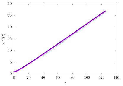
Figure 21: Evolution of second layer weights in the he weights of the second layer, as predicted by the numerical solution of Eq. (F.17). Here we use $h(z)=(9/10)z+z^{3}/6$, $\alpha=0.3$ and $\tau=0.6$. The straight line is just a guide to the eyes to test the prediction of Eq. (F.29).

Equations (F.21), (F.23) are independent of the dynamics of the second layer weights. These equations are nothing but the DMFT equations describing gradient descent dynamics of the celebrated spherical mixed $p$-spin glass model [CHS93, CK93, BADG06, FFRT20], whose definition we recall next. Consider a random cost function $H({\boldsymbol{x}})$ indexed ${\boldsymbol{x}}\in{\mathbb{S}}^{d-1}$, which is a centered Gaussian process with covariance structure given by

$$\begin{split}{\mathbb{E}}\left(H({\boldsymbol{x}})H({\boldsymbol{y}})\right)&=d\,\tilde{h}(\langle{\boldsymbol{x}},{\boldsymbol{y}}\rangle)\,.\end{split}$$ (F.24)

Define the gradient flow dynamics

$$\dot{\boldsymbol{x}}(t)=-{\boldsymbol{P}}^{\perp}_{{\boldsymbol{x}}(t)}\nabla H({\boldsymbol{x}}(t))\,,$$ (F.25)

where ${\boldsymbol{P}}^{\perp}_{{\boldsymbol{x}}(t)}$ is the projector orthogonal to ${\boldsymbol{x}}(t)$. Then the high-dimensional asymptotics of this dynamics is characterized by Eqs. (F.21), (F.23). In particular $\lim_{d\to\infty}\langle{\boldsymbol{x}}(t),{\boldsymbol{x}}(s)\rangle={\tilde{C}}^{\mbox{\tiny\rm mf}}_{d}(t,t^{\prime})$ almost surely.

A particularly interesting quantity is the asymptotic energy value in the mixed $p$-spin model:

$$\mathscrsfs{E}=\lim_{t\to\infty}\lim_{d\to\infty}\frac{1}{d}H({\boldsymbol{x}}(t))\,.$$ (F.26)

The DMFT analysis for this problem implies that

$$\mathscrsfs{E}=-\lim_{t\to\infty}\int_{0}^{t}\tilde{h}^{\prime}({\tilde{C}}^{\mbox{\tiny\rm mf}}_{d}(t,s)){\hat{R}}^{\mbox{\tiny\rm mf}}_{d}(t,s)\,{\rm d}s\>.$$ (F.27)

For $\tilde{h}(z)=c_{k}^{2}z^{k}$, $k\geq 2$, we have the explicit expression [CK93, CD95, Sel24]

$$\mathscrsfs{E}=-2c_{k}\sqrt{\frac{k-1}{k}}\,\>.$$ (F.28)

An explicit expression for $\mathscrsfs{E}$ for general covariance structure is an unknown [FFRT20].

The asymptotic energy $\mathscrsfs{E}$ has an interesting interpretation for the dynamics of two-layer networks –within the SymmDMFT theory. Eq. (F.28) implies that

$$\lim_{t\to\infty}\frac{{a}^{\mbox{\tiny\rm mf2}}(t)}{t}=-\tau\sqrt{\alpha}\mathscrsfs{E}=:A_{\infty}\,.$$ (F.29)

In Fig. 21 we test the prediction of Eq. (F.29) by integrating numerically Eqs. (F.14) to (F.17) and plotting the prediction for the second-layer weigths ${a}^{\mbox{\tiny\rm mf}}(t)$. We observe that at large $t$, ${a}^{\mbox{\tiny\rm mf2}}(t)\approx A_{\infty}t$, with $A_{\infty}$ given by Eq. (F.29)as predicted.

We also note that $C_{A}(t,t)=-\tau^{2}$ also in this timescale, and hence the train error does not change significantly. Namely , for any constant $t$, we have

$$e_{\mbox{{\rm\footnotesize tr}}}(t\sqrt{m})=\frac{1}{2}\tau^{2}+o_{m}(1)\,.$$ (F.30)

If we use heuristically Eq. (F.28) and Eq. (F.12) beyond the $\sqrt{t}$ time scale, we obtain

$$a(t)\approx{a}^{\mbox{\tiny\rm mf2}}\big{(}t/\sqrt{m}\big{)}\approx A_{\infty}\frac{t}{\sqrt{m}}\,.$$ (F.31)

This suggests that $a(t)$ becomes of order $\sqrt{m}$ on timescale of order $m$. When this happens, the network complexity is large enough to allow for interpolation, and hence we expect the dynamics to change. Indeed a new dynamical regime emerges for $t=\Theta(m)$, as we will study next.

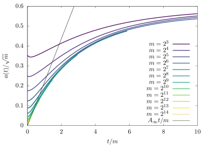
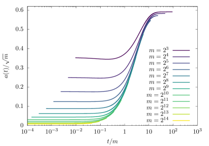
Figure 22: Training on pure noise data under mean-field initialization: $t=\Theta(m)$ regime. Rescaled second layer weights $a(t)/\sqrt{m}$ as a function of $t/m$. We plot solutions of the SymmDMFT equations for the setting of Fig. 19.

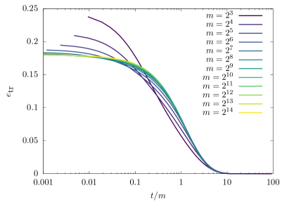
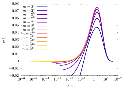
Figure 23: Train error and Lagrange multiplier $\nu(t)$ on timescales of order $m$ under mean field initialization. Solutions of the SymmDMFT equations for the setting of Fig. 19. Finite $m$ curves accumulate on master curves suggesting the existence of scaling functions.

F.1.3 Third dynamical regime: $t=\Theta(m)$

As anticipated, an additional regime arises on timescales of order $m$. In Figure 22 we plot the evolution of the weights of the second layer as a function of $t/m$ for increasing values of the width $m$. The different curves collapse suggesting the following limit to exist

$$\lim_{m\to\infty}\frac{a(tm)}{\sqrt{m}}={\gamma}^{\mbox{\tiny\rm mf3}}(t)\>.$$ (F.32)

The limit curve appears to grows linearly at small $t$, ${\gamma}^{\mbox{\tiny\rm mf3}}(t)=A_{\infty}t+o(t)$, where $A_{\infty}$ is the coefficient computed in the previous section, cf. Eq. (F.29). Hence, this third dynamical regime matches directly with the previous one. As can be seen from the right plot, there appear to be a finite limit $\lim_{t\to\infty}{\gamma}^{\mbox{\tiny\rm mf3}}(t)<\infty$.

We now turn to the analysis of the train error. Recall that on the previous timescales, the train error stays approximately constant, and equal to the train error of the null network, namely $e_{\mbox{{\rm\footnotesize tr}}}(t\sqrt{m})=\tau^{2}/2+o_{m}(1)$ for any fixed $t$. In Fig. 23 we plot both the train error and the Lagrange multiplier $\nu$ as a function of $t/m$. Again, as $m$ grows, these curve converge to limit curves. This suggests the existence of the following limits

$$\lim_{m\to\infty}e_{\mbox{{\rm\footnotesize tr}}}(tm) ={e}^{\mbox{\tiny\rm mf3}}_{\mbox{{\rm\footnotesize tr}}}(t)\,,$$ (F.33)

$$\lim_{m\to\infty}\nu(tm) ={\nu}^{\mbox{\tiny\rm mf3}}(t)\,.$$ (F.34)

Note that in this case, differently from the lazy initialization setting, the corresponding scaling function do not depend on the initialization parameter $a_{0}$.

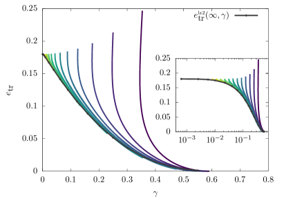
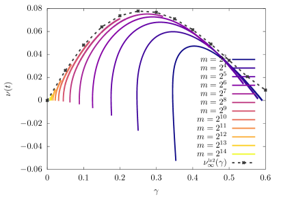
Figure 24: Train error, rescaled second-layer weights and the Lagrange multiplier $\nu(t)$ on timescales of order $m$ under mean field initialization. Left Panel: parametric plot of the train error as a function of the weights of the second layer on the scale $\sqrt{m}$, namely $\gamma=a(t)/\sqrt{m}$. The inset shows the same data on a logarithmic scale. Right Panel: same plot for the Lagrange multiplier $\nu$. Data is the same as in Fig. 19.

In order to characterize the limits in Eqs. (F.33)-(F.34), we proceed as in Sec. E.1.4. Namely, in Fig. 24 we plot the train error and the Lagrange multiplier $\nu$ as a function of the rescaled second layer weights $\gamma=a(t)/\sqrt{m}$. We also plot the asymptotic value of train error and Lagrange multiplier under the constrained GF dynamics in which second layer weigths are fixed to $a(t)=\gamma\sqrt{m}$ and do not evolve with time: ${e}^{\mbox{\tiny\rm lz2}}_{\mbox{{\rm\footnotesize tr}},\infty}(\gamma):=\lim_{t\to\infty}{e}^{\mbox{\tiny\rm lz2}}_{\mbox{{\rm\footnotesize tr}}}(t,\gamma)$ and ${\nu}^{\mbox{\tiny\rm lz2}}_{\infty}(\gamma):=\lim_{t\to\infty}{\nu}^{\mbox{\tiny\rm lz2}}(t,\gamma)$. These are computed by integration of the scaling theory in Section E.1.2.

The good collapse on these curves suggests to consider the the following construction, analogous to Sec. E.1.4. Define the inverse function of $t\mapsto{\gamma}^{\mbox{\tiny\rm mf3}}(t)$, denoted by $({\gamma}^{\mbox{\tiny\rm mf3}})^{-1}$. Then, define

$$\begin{split}{\varepsilon}^{\mbox{\tiny\rm mf3}}(\gamma)&={e}^{\mbox{\tiny\rm mf3}}_{\mbox{{\rm\footnotesize tr}}}(({\gamma}^{\mbox{\tiny\rm mf3}})^{-1}(\gamma))\,,\\ {\nu}^{\mbox{\tiny\rm mf3}}_{*}(\gamma)&={\nu}^{\mbox{\tiny\rm mf3}}(({\gamma}^{\mbox{\tiny\rm mf3}})^{-1}(\gamma))\,.\end{split}$$ (F.35)

Figure 24 suggests that

$${\varepsilon}^{\mbox{\tiny\rm mf3}}(\gamma) \approx{e}^{\mbox{\tiny\rm lz2}}_{\mbox{{\rm\footnotesize tr}},\infty}(\gamma)\,,$$ (F.36)

$${\nu}^{\mbox{\tiny\rm mf3}}_{*}(\gamma) \approx{\nu}^{\mbox{\tiny\rm lz2}}_{\mbox{{\rm\footnotesize tr}},\infty}(\gamma)\,.$$ (F.37)

Equations (F.36), (F.36) imply that on timescales of order $m$ the dynamics is adiabatic. For each incremental change of $a$ on a the scale $\sqrt{m}$, all one-time quantities relax to the asymptotic value which turns out to be the same as a constrained model with $a(t)/\sqrt{m}=\gamma$ fixed.

The consequence of Eqs. (F.36)-(F.36) is that

$$\lim_{t\to\infty}{\gamma}^{\mbox{\tiny\rm mf3}}(t)\approx\gamma_{\rm GF}^{*}(\alpha,\tau)\,.$$ (F.38)

where $\gamma_{\rm GF}^{*}(\alpha,\tau)$ corresponds to the interpolation value of the initialization scale of a lazy model.

F.2 Multi-index model

In this section we consider the case in which the dataset is distributed according to a multi-index model. For time scales beyond $t=O(1)$, we will assume that $h(z)=\hat{\varphi}(z)$. This simplifies the asymptotics for $t$ large but of order one.

We identify two dynamical regimes emerging as $m\to\infty$:

• $t=O(1)$: $a(t)=O(1)$ but is not constant. Also, the projection ${\boldsymbol{v}}(t)$ of first layer weights onto the latent space evolve as well as do train and test error. We further have $e_{\mbox{{\rm\footnotesize tr}}}(t)=e_{\mbox{\rm\footnotesize ts}}(t)+o_{m}(1)$: there is no overfitting. This evolution is captured the mean field theory of [MMN18, CB18] which we recover as $m\to\infty$ limit of SymmDMFT .

• $t=\Theta(m)$: $a(t)=\Theta(\sqrt{m})$, ${\boldsymbol{v}}(t)$ decreases towards $0$ and train and test error diverge. In this dynamical regime the network unlearns to a large extent the latent structure of the data and overfit it.

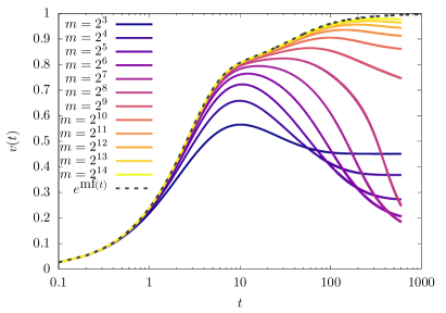
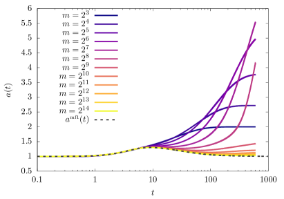
Figure 25: Gradient flow dynamics under mean field initialization in the first dynamical regime $t=O(1)$. for data distributed according to a single index model. Curves are numerical solutions of the SymmDMFT equations: we plot $v(t)$ and $a(t)$ for different values of $m$ and compare them to the mean field predictions. Data is distributed according to a single index model with $h_{t}(z)=\hat{\varphi}(z)=h(z)=(9/10)z+z^{3}/6$ with $\tau=0.6$ and $\alpha=0.3$.

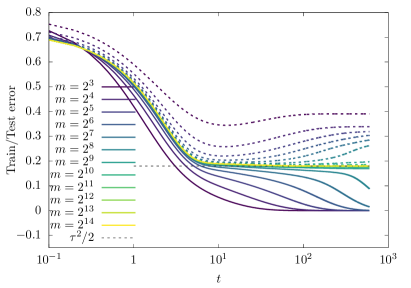
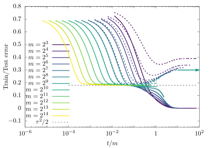
Figure 26: Gradient flow dynamics under mean field initialization $a(0)=1$. The train (solid curves) and test (dashed curves) errors as a function of time $t$ (left panel) and scaled time $t/m$ (right panel). Curves are numerical solutions of the SymmDMFT equations for $h(z)=(9/10)z+z^{3}/6$, $\hat{\varphi}(z)=h(z)$, $\tau=0.6$ and $\alpha=0.3$. The arrow on the right panel corresponds to the asymptotic test error for a model with second layer weights fixed to the corresponding interpolation threshold.

F.2.1 First dynamical regime: $t=\Theta(1)$

For timescales of order one, the SymmDMFT equations are solved, up to subleading terms as $m\to\infty$, by the following ansatz

$$C_{d}(t,s) ={C}^{\mbox{\tiny\rm mf1}}_{d}(t,s)+o_{m}(1)\,, C_{o}(t,s) ={C}^{\mbox{\tiny\rm mf1}}_{o}(t,s)+o_{m}(1)\,,$$ (F.39)

$$R_{d}(t,s) ={R}^{\mbox{\tiny\rm mf1}}_{d}(t,s)+o_{m}(1)\,, mR_{o}(t,s) ={R}^{\mbox{\tiny\rm mf1}}_{o}(t,s)+o_{m}(1)$$ (F.40)

$$v(t) ={v}^{\mbox{\tiny\rm mf1}}(t)+o_{m}(1)\,, a(t) ={a}^{\mbox{\tiny\rm mf1}}(t)\,.$$ (F.41)

The corresponding scaling equations are then given by

$$\begin{split}\partial_{t}{R}^{\mbox{\tiny\rm mf1}}_{o}(t,t^{\prime})&=-{\nu}^{\mbox{\tiny\rm mf1}}(t){R}^{\mbox{\tiny\rm mf1}}_{o}(t,t^{\prime})-\alpha{a}^{\mbox{\tiny\rm mf1}}(t)^{2}h^{\prime}({C}^{\mbox{\tiny\rm mf1}}_{o}(t,t))\left({R}^{\mbox{\tiny\rm mf1}}_{d}(t,t^{\prime})+{R}^{\mbox{\tiny\rm mf1}}_{o}(t,t^{\prime})\right)\,,\\ \partial_{t}{C}^{\mbox{\tiny\rm mf1}}_{o}(t,t^{\prime})&=-{\nu}^{\mbox{\tiny\rm mf1}}(t){C}^{\mbox{\tiny\rm mf1}}_{o}(t,t^{\prime})+\alpha\langle\nabla\hat{\varphi}({{\boldsymbol{v}}}^{\mbox{\tiny\rm mf1}}(t)),{{\boldsymbol{v}}}^{\mbox{\tiny\rm mf1}}(t^{\prime})\rangle{a}^{\mbox{\tiny\rm mf1}}(t)-\alpha{a}^{\mbox{\tiny\rm mf1}}(t)^{2}h^{\prime}({C}^{\mbox{\tiny\rm mf1}}_{o}(t,t)){C}^{\mbox{\tiny\rm mf1}}_{o}(t,t^{\prime})\,,\\ {\nu}^{\mbox{\tiny\rm mf1}}(t)&=\alpha\langle\nabla\hat{\varphi}({{\boldsymbol{v}}}^{\mbox{\tiny\rm mf1}}(t)),{{\boldsymbol{v}}}^{\mbox{\tiny\rm mf1}}(t)\rangle{a}^{\mbox{\tiny\rm mf1}}(t)-\alpha{a}^{\mbox{\tiny\rm mf1}}(t)^{2}h^{\prime}({C}^{\mbox{\tiny\rm mf1}}_{o}(t,t)){C}^{\mbox{\tiny\rm mf1}}_{o}(t,t)\\ \partial_{t}{C}^{\mbox{\tiny\rm mf1}}_{d}(t,t^{\prime})&=-{\nu}^{\mbox{\tiny\rm mf1}}(t){C}^{\mbox{\tiny\rm mf1}}_{d}(t,t^{\prime})+\alpha\langle\nabla\hat{\varphi}({{\boldsymbol{v}}}^{\mbox{\tiny\rm mf1}}(t)),{{\boldsymbol{v}}}^{\mbox{\tiny\rm mf1}}(t^{\prime})\rangle{a}^{\mbox{\tiny\rm mf1}}(t)-\alpha{a}^{\mbox{\tiny\rm mf1}}(t)^{2}h^{\prime}({C}^{\mbox{\tiny\rm mf1}}_{o}(t,t)){C}^{\mbox{\tiny\rm mf1}}_{o}(t,t^{\prime})\,,\\ \partial_{t}{R}^{\mbox{\tiny\rm mf1}}_{d}(t,t^{\prime})&=-{\nu}^{\mbox{\tiny\rm mf1}}(t){R}^{\mbox{\tiny\rm mf1}}_{d}(t,t^{\prime})+\delta(t-t^{\prime})\,,\\ \partial_{t}{{\boldsymbol{v}}}^{\mbox{\tiny\rm mf1}}(t)&=-{\nu}^{\mbox{\tiny\rm mf1}}(t){{\boldsymbol{v}}}^{\mbox{\tiny\rm mf1}}(t)+\alpha\nabla\hat{\varphi}({{\boldsymbol{v}}}^{\mbox{\tiny\rm mf1}}(t)){a}^{\mbox{\tiny\rm mf1}}(t)-\alpha{a}^{\mbox{\tiny\rm mf1}}(t)^{2}h^{\prime}({C}^{\mbox{\tiny\rm mf1}}_{o}(t,t)){{\boldsymbol{v}}}^{\mbox{\tiny\rm mf1}}(t)\,,\\ \partial_{t}{a}^{\mbox{\tiny\rm mf1}}(t)&=\alpha\left(\hat{\varphi}({{\boldsymbol{v}}}^{\mbox{\tiny\rm mf1}}(t))-{a}^{\mbox{\tiny\rm mf1}}(t)h({C}^{\mbox{\tiny\rm mf1}}_{o}(t,t))\right)\,.\end{split}$$ (F.42)

These equations are solved by setting:

$${C}^{\mbox{\tiny\rm mf1}}_{o}(t,t^{\prime})=\langle{{\boldsymbol{v}}}^{\mbox{\tiny\rm mf1}}(t),{{\boldsymbol{v}}}^{\mbox{\tiny\rm mf1}}(t^{\prime})\rangle$$ (F.43)

with ${{\boldsymbol{v}}}^{\mbox{\tiny\rm mf1}}(t)$, ${a}^{\mbox{\tiny\rm mf1}}(t)$ the solution of

$$\begin{split}\partial_{t}{{\boldsymbol{v}}}^{\mbox{\tiny\rm mf1}}(t)&=\alpha{a}^{\mbox{\tiny\rm mf1}}(t)\big{(}{\boldsymbol{I}}_{k}-{{\boldsymbol{v}}}^{\mbox{\tiny\rm mf1}}(t){{\boldsymbol{v}}}^{\mbox{\tiny\rm mf1}}(t)^{{\sf T}}\big{)}\left(\nabla\hat{\varphi}({{\boldsymbol{v}}}^{\mbox{\tiny\rm mf1}}(t))-{a}^{\mbox{\tiny\rm mf1}}(t)h^{\prime}(\|{{\boldsymbol{v}}}^{\mbox{\tiny\rm mf1}}(t)\|^{2}){{\boldsymbol{v}}}^{\mbox{\tiny\rm mf1}}(t)\right)\,,\\ \partial_{t}{a}^{\mbox{\tiny\rm mf1}}(t)&=\alpha\left(\hat{\varphi}({{\boldsymbol{v}}}^{\mbox{\tiny\rm mf1}}(t))-{a}^{\mbox{\tiny\rm mf1}}(t)h(\|{{\boldsymbol{v}}}^{\mbox{\tiny\rm mf1}}(t)\|^{2})\right)\,,\end{split}$$ (F.44)

with initial conditions given by ${{\boldsymbol{v}}}^{\mbox{\tiny\rm mf1}}(0)={\mathbf{0}}$ and ${a}^{\mbox{\tiny\rm mf1}}(0)=a_{0}$.

Equations (F.44) coincide with the mean field theory of [MMN18, CB18, RVE22], when the latter are specialized to the multi-index model studied here, under symmetric initializations [BMZ24, Section 4.2]. (See also [ASKL23].) Using the ansatz of Eqs. (F.39) to (F.41) in the formulas for training and test error (B.45), (B.46), we get

$$\lim_{m\to\infty}e_{\mbox{{\rm\footnotesize tr}}}(t)=\lim_{m\to\infty}e_{\mbox{\rm\footnotesize ts}}(t)={e}^{\mbox{\tiny\rm mf1}}(t)\,,$$ (F.45)

with

$${e}^{\mbox{\tiny\rm mf1}}(t)=\frac{1}{2}\left[\tau^{2}+\|\varphi\|^{2}-2{a}^{\mbox{\tiny\rm mf1}}(t)\hat{\varphi}({{\boldsymbol{v}}}^{\mbox{\tiny\rm mf1}}(t))+{a}^{\mbox{\tiny\rm mf1}}(t)^{2}h(\|{{\boldsymbol{v}}}^{\mbox{\tiny\rm mf1}}(t)\|^{2})\right]\,.$$ (F.46)

A particularly simple case is the one in which $k=1$ (single index model) and $\varphi=\sigma$ (whence $\hat{\varphi}=h$). For a class of such activations with $h^{\prime}(0)>0$, we have ${a}^{\mbox{\tiny\rm mf1}}(t),{v}^{\mbox{\tiny\rm mf1}}(t)\to 1$ as $t\to\infty$ and therefore

$$\lim_{t\to\infty}{e}^{\mbox{\tiny\rm mf1}}(t)=\frac{\tau^{2}}{2}\,.$$ (F.47)

In other words, neurons align perfectly with latent direction, the generalization error vanishes, and and train and test error converge for large constant $t$ to the Bayes error $\tau^{2}/2$.

In Fig. 25 we compare the solution of Eqs. (F.44) with the numerical integrations of the SymmDMFT equations for a range of values of $m$. As $m$ increases, the SymmDMFT solutions converge to the asymptotic predictions ${v}^{\mbox{\tiny\rm mf1}}(t)$, ${a}^{\mbox{\tiny\rm mf1}}(t)$, confirming the above ansatz.

Similarly, in Fig. 26-left panel we compute the train and test error by solving the SymmDMFT equations and compare the results to the asymptotic prediction provided by Eq. (F.46). We observe that –as predicted– train and test error match on an increasingly long time interval. At a certain point, they diverge: we will next characterize the timescale on which this happens.

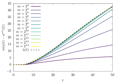
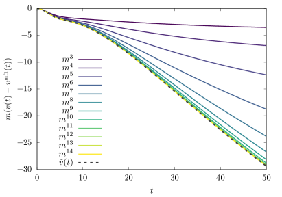
Figure 27: The $1/m$ corrections to the second layer weights and the projection on the latent space of the single index model on timescales of order $1$. Dashed lines are obtained by integrating numerically Eqs. (F.56) to (F.59) determining the limits $m\to\infty$. Here, $\hat{\varphi}(z)=h(z)=(9/10)z+z^{3}/6$ with $\tau=0.6$ and $\alpha=0.3$.

F.2.2 Escape from the mean field dynamical regime

In order to understand on which time scale the dynamics diverges from mean field theory described above, we will study small deviations from this theory. We expect that these deviations will diverge with time. Characterizing this divergence will allow to determine time scale on which we exit the mean field regime.

We focus on the case of a single index model $k=1$, with $\hat{\varphi}=h$, and set $a(0)=1$. We believe that the qualitative conclusions obtained in this case apply more generally. We also assume $h$ to be such that the long time asymptotics of mean field dynamical solutions is

$$\lim_{t\to\infty}{a}^{\mbox{\tiny\rm mf1}}(t) =1\,,\;\;\;\;\;\;\;\;\;\lim_{t\to\infty}{v}^{\mbox{\tiny\rm mf1}}(t)=1\>.$$ (F.48)

As mentioned in the previous section, this holds for a broad class of activations. In other words, for time $t$ large and yet of order one, the neurons are very well aligned.

We next study the corrections to the mean field solution. We claim that such corrections are of order $1/m$ and define the functions $\tilde{a}(t)$, $\tilde{v}(t)$, dots ,$\tilde{R}_{o}(t,t^{\prime})$, via

$$m(a(t)-{a}^{\mbox{\tiny\rm mf1}}(t))=\tilde{a}(t)+o_{m}(1)\,,$$ (F.49)

$$m(v(t)-{v}^{\mbox{\tiny\rm mf1}}(t))=\tilde{v}(t)+o_{m}(1)\,,$$ (F.50)

$$m(C_{d}(t,t^{\prime})-{C}^{\mbox{\tiny\rm mf1}}_{d}(t,t^{\prime}))=\tilde{C}_{d}(t,t^{\prime})+o_{m}(1)\,,$$ (F.51)

$$m(C_{o}(t,t^{\prime})-{C}^{\mbox{\tiny\rm mf1}}_{o}(t,t^{\prime}))=\tilde{C}_{o}(t,t^{\prime})+o_{m}(1)\,,$$ (F.52)

$$m(R_{d}(t,t^{\prime})-{R}^{\mbox{\tiny\rm mf1}}_{d}(t,t^{\prime}))=\tilde{R}_{d}(t,t^{\prime})+o_{m}(1)\,,$$ (F.53)

$$m(R_{o}(t,t^{\prime})-{R}^{\mbox{\tiny\rm mf1}}_{o}(t,t^{\prime}))=\tilde{R}_{o}(t,t^{\prime})+o_{m}(1)\,,$$ (F.54)

$$m(\nu(t)-{\nu}^{\mbox{\tiny\rm mf1}}(t))=\tilde{\nu}(t)+o_{m}(1)\,.$$ (F.55)

Substituting the above form into the SymmDMFT equations and matching the next-to-leading order in $m$ we can obtain the equations for the $1/m$ corrections. It turns out that equations for $\tilde{a},\ \tilde{v},\ \tilde{C}_{o}$ and $\tilde{\nu}$ decouple from the equations for $\tilde{C}_{d}$, $\tilde{R}_{d}$ and $\tilde{R}_{o}$. Given that we are interested in the former quantities we only report the corresponding equations:

$$\frac{{\rm d}\tilde{a}(t)}{{\rm d}t}= \alpha\hat{\varphi}^{\prime}({v}^{\mbox{\tiny\rm mf1}}(t))\tilde{v}(t)-\alpha\hat{\varphi}({v}^{\mbox{\tiny\rm mf1}}(t))\int_{0}^{t}\Sigma_{R}^{(1)}(t,s)\,{\rm d}s-\alpha{a}^{\mbox{\tiny\rm mf1}}(t)\left[h(1)-h({C}^{\mbox{\tiny\rm mf1}}_{o}(t,t))\right]$$ (F.56)

$$+\alpha\int_{0}^{t}\Sigma_{R}^{(1)}(t,s){a}^{\mbox{\tiny\rm mf1}}(s)h({C}^{\mbox{\tiny\rm mf1}}_{o}(t,s)){\rm d}s-\alpha\tilde{a}(t)h({C}^{\mbox{\tiny\rm mf1}}_{o}(t,t))-\alpha{a}^{\mbox{\tiny\rm mf1}}(t)h^{\prime}({C}^{\mbox{\tiny\rm mf1}}_{o}(t,t))\tilde{C}_{o}(t,t)$$

$$-\alpha\int_{0}^{t}{C}^{\mbox{\tiny\rm mf1}}_{A}(t,s){a}^{\mbox{\tiny\rm mf1}}(s)\left[h^{\prime}({C}^{\mbox{\tiny\rm mf1}}_{d}(t,s)){R}^{\mbox{\tiny\rm mf1}}_{d}(t,s)+h^{\prime}({C}^{\mbox{\tiny\rm mf1}}_{o}(t,s)){R}^{\mbox{\tiny\rm mf1}}_{o}(t,s)\right]\,{\rm d}s\,,$$

$$\frac{{\rm d}\tilde{v}(t)}{{\rm d}t}= -{\nu}^{\mbox{\tiny\rm mf1}}(t)\tilde{v}(t)-\tilde{\nu}(t){v}^{\mbox{\tiny\rm mf1}}(t)+\alpha\hat{\varphi}({v}^{\mbox{\tiny\rm mf1}}(t))\tilde{a}(t)+\alpha\hat{\varphi}^{\prime\prime}({v}^{\mbox{\tiny\rm mf1}}(t))\tilde{v}(t){a}^{\mbox{\tiny\rm mf1}}(t)$$ (F.57)

$$-\alpha\hat{\varphi}^{\prime}({v}^{\mbox{\tiny\rm mf1}}(t)){a}^{\mbox{\tiny\rm mf1}}(t)\int_{0}^{t}\Sigma^{(1)}_{R}(t,s)\,{\rm d}s-\int_{0}^{t}\left[\tilde{M}_{R}^{(d)}(t,s)-M_{R,o}^{(0)}(t,s)\right]{v}^{\mbox{\tiny\rm mf1}}(s)\,{\rm d}s$$

$$-\int_{0}^{t}\left[M_{R,o}^{(1)}(t,s){v}^{\mbox{\tiny\rm mf1}}(s)+M_{R,o}^{(0)}(t,s)\tilde{v}(s)\right]\,{\rm d}s\,,$$

$$\tilde{\nu}(t)= \alpha\hat{\varphi}^{\prime}({v}^{\mbox{\tiny\rm mf1}}(t))\tilde{v}(t){a}^{\mbox{\tiny\rm mf1}}(t)+\alpha\hat{\varphi}^{\prime\prime}({v}^{\mbox{\tiny\rm mf1}}(t)){v}^{\mbox{\tiny\rm mf1}}(t)\tilde{v}(t){a}^{\mbox{\tiny\rm mf1}}(t)$$ (F.58)

$$+\alpha\hat{\varphi}^{\prime}({v}^{\mbox{\tiny\rm mf1}}(t)){v}^{\mbox{\tiny\rm mf1}}(t)\tilde{a}(t)-\alpha\hat{\varphi}^{\prime}({v}^{\mbox{\tiny\rm mf1}}(t)){v}^{\mbox{\tiny\rm mf1}}(t)\int_{0}^{t}\Sigma_{R}^{(1)}(t,s)\,{\rm d}s$$

$$-\int_{0}^{t}\left[\tilde{M}_{R}^{(d)}(t,s){C}^{\mbox{\tiny\rm mf1}}_{d}(t,s)-M_{R,o}^{(0)}(t,s){C}^{\mbox{\tiny\rm mf1}}_{o}(t,s)\right]\,{\rm d}s$$

$$-\int_{0}^{t}\left[M_{R,o}^{(1)}(t,s){C}^{\mbox{\tiny\rm mf1}}_{o}(t,s)+M_{R,o}^{(0)}(t,s)\tilde{C}_{o}(t,s)\right]\,{\rm d}s$$

$$-\int_{0}^{t}\left[\tilde{M}_{C}^{(d)}(t,s){R}^{\mbox{\tiny\rm mf1}}_{d}(t,s)+M_{C,o}^{(0)}(t,s){R}^{\mbox{\tiny\rm mf1}}_{o}(t,s)\right]\,{\rm d}s\,,$$

$$\frac{\partial\tilde{C}_{o}(t,t^{\prime})}{\partial t}= -{\nu}^{\mbox{\tiny\rm mf1}}(t)\tilde{C}_{o}(t,t^{\prime})-\tilde{\nu}(t){C}^{\mbox{\tiny\rm mf1}}_{o}(t,t^{\prime})+\alpha\hat{\varphi}^{\prime\prime}({v}^{\mbox{\tiny\rm mf1}}(t))\tilde{v}(t){v}^{\mbox{\tiny\rm mf1}}(t^{\prime}){a}^{\mbox{\tiny\rm mf1}}(t)$$ (F.59)

$$+\alpha\hat{\varphi}^{\prime}({v}^{\mbox{\tiny\rm mf1}}(t))\tilde{v}(t^{\prime}){a}^{\mbox{\tiny\rm mf1}}(t)+\alpha\hat{\varphi}^{\prime}({v}^{\mbox{\tiny\rm mf1}}(t)){v}^{\mbox{\tiny\rm mf1}}(t^{\prime})\tilde{a}(t)$$

$$-\alpha\hat{\varphi}^{\prime}({v}^{\mbox{\tiny\rm mf1}}(t)){v}^{\mbox{\tiny\rm mf1}}(t^{\prime}){a}^{\mbox{\tiny\rm mf1}}(t)\int_{0}^{t}\Sigma_{R}^{(1)}(t,s)\,{\rm d}s$$

$$-\int_{0}^{t}\left[\tilde{M}_{R}^{(d)}(t,s){C}^{\mbox{\tiny\rm mf1}}_{o}(t^{\prime},s)+M_{R,o}^{(0)}(t,s){C}^{\mbox{\tiny\rm mf1}}_{d}(t^{\prime},s)-2M_{R,o}^{(0)}(t,s){C}^{\mbox{\tiny\rm mf1}}_{o}(t^{\prime}s)\right]\,{\rm d}s$$

$$-\int_{0}^{t}\left[M_{R,o}^{(0)}(t,s)\tilde{C}_{o}(t^{\prime},s)+M_{R,o}^{(1)}(t,s){C}^{\mbox{\tiny\rm mf1}}_{o}(t^{\prime},s)\right]\,{\rm d}s$$

$$-\int_{0}^{t^{\prime}}\left[\tilde{M}_{C}^{(d)}(t,s){R}^{\mbox{\tiny\rm mf1}}_{d}(t^{\prime},s)+M_{C,o}^{(0)}(t,s){R}^{\mbox{\tiny\rm mf1}}_{o}(t^{\prime},s)\right]\,{\rm d}s\>.$$

Here, we used the following auxiliary functions

$$\Sigma_{R}^{(1)}(t,s) ={a}^{\mbox{\tiny\rm mf1}}(t){a}^{\mbox{\tiny\rm mf1}}(s)\left[h^{\prime}({C}^{\mbox{\tiny\rm mf1}}_{d}(t,s)){R}^{\mbox{\tiny\rm mf1}}_{d}(t,s)+h^{\prime}({C}^{\mbox{\tiny\rm mf1}}_{o}(t,s)){R}^{\mbox{\tiny\rm mf1}}_{o}(t,s)\right]\,,$$ (F.60)

$${C}^{\mbox{\tiny\rm mf1}}_{A}(t,s) =-\left[\tau^{2}+h_{t}(1)-{a}^{\mbox{\tiny\rm mf1}}(t)\varphi({v}^{\mbox{\tiny\rm mf1}}(t))-{a}^{\mbox{\tiny\rm mf1}}(s)\varphi({v}^{\mbox{\tiny\rm mf1}}(s))+{a}^{\mbox{\tiny\rm mf1}}(t){a}^{\mbox{\tiny\rm mf1}}(s)h({C}^{\mbox{\tiny\rm mf1}}_{o}(t,s))\right]\,,$$ (F.61)

$$\tilde{M}_{R}^{(d)}(t,s) =\alpha{a}^{\mbox{\tiny\rm mf1}}(t){a}^{\mbox{\tiny\rm mf1}}(s)\left[h^{\prime}(1)\delta(t-s)+{C}^{\mbox{\tiny\rm mf1}}_{A}(t,s)h^{\prime\prime}({C}^{\mbox{\tiny\rm mf1}}_{d}(t,s)){R}^{\mbox{\tiny\rm mf1}}_{d}(t,s)\right]\,,$$ (F.62)

$$M_{R,o}^{(0)}(t,s) =\alpha({a}^{\mbox{\tiny\rm mf1}}(t))^{2}h^{\prime}({C}^{\mbox{\tiny\rm mf1}}_{o}(t,s))\delta(t-s)\,,$$ (F.63)

$$M_{R,o}^{(1)}(t,s) =\alpha\left[2{a}^{\mbox{\tiny\rm mf1}}(t)\tilde{a}(t)h^{\prime}({C}^{\mbox{\tiny\rm mf1}}_{o}(t,t))+({a}^{\mbox{\tiny\rm mf1}}(t))^{2}h^{\prime\prime}({C}^{\mbox{\tiny\rm mf1}}_{o}(t,t))\tilde{C}(t,t)\right]\delta(t-s)$$ (F.64)

$$-\alpha{a}^{\mbox{\tiny\rm mf1}}(t){a}^{\mbox{\tiny\rm mf1}}(s)\Sigma_{R}^{(1)}(t,s)h^{\prime}({C}^{\mbox{\tiny\rm mf1}}_{o}(t,s))$$ (F.65)

$$+\alpha{a}^{\mbox{\tiny\rm mf1}}(t){a}^{\mbox{\tiny\rm mf1}}(s){C}^{\mbox{\tiny\rm mf1}}_{A}(t,s)h^{\prime\prime}({C}^{\mbox{\tiny\rm mf1}}_{o}(t,s)){R}^{\mbox{\tiny\rm mf1}}_{o}(t,s)\,,$$ (F.66)

$$\tilde{M}_{C}^{(d)}(t,s) =\alpha{a}^{\mbox{\tiny\rm mf1}}(t){a}^{\mbox{\tiny\rm mf1}}(s){C}^{\mbox{\tiny\rm mf1}}_{A}(t,s)h^{\prime}({C}^{\mbox{\tiny\rm mf1}}_{d}(t,s))\,,$$ (F.67)

$$M_{C,o}^{(0)}(t,s) =\alpha{a}^{\mbox{\tiny\rm mf1}}(t){a}^{\mbox{\tiny\rm mf1}}(s){C}^{\mbox{\tiny\rm mf1}}_{A}(t,s)h^{\prime}({C}^{\mbox{\tiny\rm mf1}}_{o}(t,s))\,.$$ (F.68)

Note that Eqs. (F.56) to (F.59) are a set of four integral-differential equations for the four functions $\tilde{a}(t)$, $\tilde{v}(t)$, $\tilde{\nu}(t)$, $\tilde{C}_{o}(t,t^{\prime})$. The original SymmDMFT equations involve three other functions: $\tilde{C}_{d}(t,t^{\prime})$, $\tilde{R}_{d}(t,t^{\prime})$, $\tilde{R}_{o}(t,t^{\prime})$? We also remark that: $(i)$ These equations are linear in the unknowns $\tilde{a}(t)$, $\tilde{v}(t)$, $\tilde{\nu}(t)$, $\tilde{C}_{o}(t,t^{\prime})$; $(ii)$ They can be integrated numerically with the same strategy used to integrate the SymmDMFT equations.

In Fig. 27 we plot the deviations from the mean field limit $m(a(t)-{a}^{\mbox{\tiny\rm mf1}}(t))$ and $m(v(t)-{v}^{\mbox{\tiny\rm mf1}}(t))$ as a function of time $t$, as obtained by solving the SymmDMFT equations, for several values of $m$. We also plot the predicted limits $\tilde{a}(t)$, $\tilde{v}(t)$, which are obtained by integrating Eqs. (F.56) to (F.59) As $m$ gets large, the finite-$m$ curves appear to converge to the predictions $\tilde{a}(t)$, $\tilde{v}(t)$.

In Figure 28 we plot the result of integrating Eqs. (F.56) to (F.59) over a wider time window. We observe that $\tilde{v}$, $\tilde{a}$, $\tilde{\nu}$ and $\tilde{C}_{o}(t,t)$ diverge linearly with $t$.

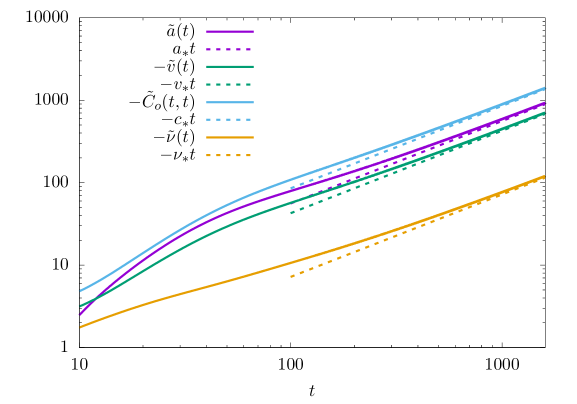
Figure 28: The $1/m$ corrections to $v(t)$, $a(t)$, $C_{o}(t,t)$ and $\tilde{\nu}(t)$ as a function of time as extracted from the numerical integration of the corresponding equations. The dashed lines are the asymptotic predictions for $t\to\infty$ which show that the divergence of all quantities is linear with time. Here, $\hat{\varphi}(z)=h(z)=(9/10)z+z^{3}/6$ with $\tau=0.6$ and $\alpha=0.3$.

This suggests the following asymptotics for these corrections

$$\lim_{t\to\infty}\frac{\tilde{a}(t)}{t} =a_{*}\,, \lim_{t\to\infty}\frac{\tilde{v}(t)}{t} =v_{*}\,,$$ (F.69)

$$\lim_{t\to\infty}\frac{\tilde{\nu}(t)}{t} =\nu_{*}\,, \lim_{t\to\infty}\frac{\tilde{C}_{o}(t,t)}{t} =c_{*}\,.$$ (F.70)

The values of the constant $a_{*}$, $v_{*}$, $\nu_{*}$ and $c_{*}$ can be obtained analytically by using the above ansatz in Eqs. (F.56) to (F.59). We obtain that they solve the following linear equations

$$0 =\hat{\varphi}^{\prime}(1)v_{*}+{\hat{\varphi}(1)}a_{*}\,,$$ (F.71)

$$0 =\hat{\varphi}^{\prime}(1)c_{*}+2{\hat{\varphi}(1)}a_{*}\,,$$ (F.72)

$$0 =-\hat{\varphi}^{\prime}(1)\nu_{*}-\hat{\varphi}^{\prime}(1)\left(\alpha\hat{\varphi}^{\prime\prime}(1)-\alpha\hat{\varphi}^{\prime}(1)-\alpha(\hat{\varphi}^{\prime}(1))^{2}\right)a_{*}+2\alpha\hat{\varphi}(1)\hat{\varphi}^{\prime\prime}(1)\,,$$ (F.73)

$$0 =-\frac{1}{2}c_{*}-\nu_{1}c_{*}-2\nu_{*}v_{1}+4v_{1}\alpha\tau^{2}\,,$$ (F.74)

where

$$v_{1} :=\lim_{t\to\infty}(v(t)-1)t\,,$$ (F.75)

$$\nu_{1} :=\lim_{t\to\infty}\tilde{\nu}(t)t\,.$$ (F.76)

The asymptotic linear behavior predicted by Eqs. (F.69), (F.70), with the coefficients determined by Eqs. (F.71)-(F.74) is plotted in Fig. 28. We observe good agreement with the numerical integration of Eqs. (F.56) to (F.59).

The above analysis implies that (considering to be definite second layer weights, and projection of first layer weigths onto the latent direction), for $m\gg 1$, $t\gg 1$,

$$a(t) ={a}^{\mbox{\tiny\rm mf1}}(t)+\frac{1}{m}\big{(}a_{*}t+o(t)\big{)}+\frac{1}{m}\Delta_{a}(t,m)\,,$$ (F.77)

$$v(t) ={v}^{\mbox{\tiny\rm mf1}}(t)+\frac{1}{m}\big{(}v_{*}t+o(t)\big{)}+\frac{1}{m}\Delta_{v}(t,m)\,,$$ (F.78)

where $\lim_{m\to\infty}\Delta_{a/v}(t,m)=0$. If we neglect the error terms, and assume that this expression holds for $t$ larger than $O(1)$ in $m$, then it indicates that $a(t)$, $v(t)$ differ significantly from the mean field prediction when $t/m$ becomes of order one. We expect therefore a third dynamical regime for $t=\Theta(m)$, which will be the object of the next section.

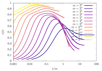
Figure 29: Gradient flow under mean field initialization on timescales of order $m$. Left: rescaled second layer weights $a(t)/m$ as a function of the rescaled time $t/m$. The arrow on the right points at the threshold $\gamma_{\mbox{\tiny\rm GF}}^{*}(\alpha,\varphi,\tau)$ for interpolation under gradient flow, see Section E.2.3. Right: projection of the first layer weights on the latent space in the single index model as a function of rescaled time $t/m$. Here, $\hat{\varphi}(z)=h(z)=(9/10)z+z^{3}/6$ with $\tau=0.6$ and $\alpha=0.3$. $v=1/\gamma$ in (E.57).

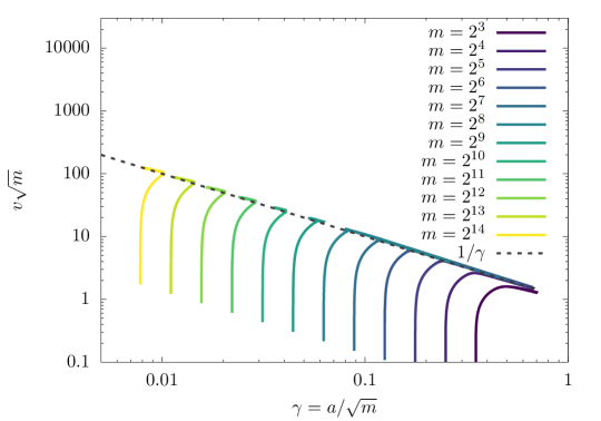
Figure 30: Same data as in Fig. 29: parametric plot of the rescaled projection onto the latent direction $v\sqrt{m}$ against rescaled second layer weights $\gamma=a/\sqrt{m}$. Dashed line is $v\sqrt{m}=1/\gamma$.

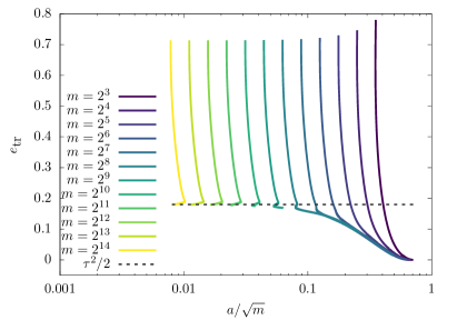
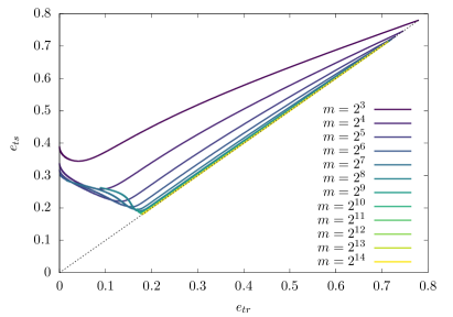
Figure 31: Gradient flow under mean field initialization, for increasing values of $m$. Left: train error as a function of rescaled weights $a(t)/\sqrt{m}$. Dashed line is the Bayes error $\tau^{2}/2$. Curves are traversed in time from top to bottom. Right: test error versus train error. Curves are traversed in time from right to left. Here $\hat{\varphi}(z)=h(z)=(9/10)z+z^{3}/6$ with $\tau=0.6$ and $\alpha=0.3$.

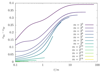
Figure 32: Left panel: the difference between test and train error plotted as a function of $a/\sqrt{m}$ and compared to what is obtained from a model with fixed second layer weights initialized with Lazy scaling. Right panel: the difference between test and train error on timescales of order $m$. Here, $\hat{\varphi}(z)=h(z)=(9/10)z+z^{3}/6$ with $\tau=0.6$ and $\alpha=0.3$.

F.2.3 Second dynamical regime: $t=\Theta(m)$ and beyond

As pointed out at the end of the previous section, we expect a third dynamical regime when $t=\Theta(m)$. By this time, the stability calculation in the previous section indicates that second layer weights become of order $\sqrt{m}$. Figure 29 confirms this, and shows that, in the same regime $v(t)$ becomes small. In fact, numerical solution of the SymmDMFT equations are consistent with $a(t)=\Theta(\sqrt{m})$, $v(t)=\Theta(1/\sqrt{m})$, and $a(t)v(t)\approx 1$ for $t=\Theta(m)$.

For a small constant $c$ denote by $t_{0}(m;c)$ the time at which $a(t_{0}(m;c))=c\sqrt{m}$. We then expect that the following exists

$$\lim_{m\to\infty}\frac{a(t_{0}(m;c)+\theta\,w(m))}{\sqrt{m}} ={\gamma}^{\mbox{\tiny\rm mf3}}(\theta)\,,$$ (F.79)

$$\lim_{m\to\infty}{\boldsymbol{v}}(t_{0}(m;c)+\theta\,w(m))\sqrt{m} ={{\boldsymbol{v}}}^{+}(\theta)\,,$$ (F.80)

provided $w(m)$ is a suitable function (with $w(m)=O(t_{0}(m;c))$). The stability analysis in the previous section suggests that $t_{0}(m;c)\leq t_{*}(c)m+o(m)$. Our numerical solutions do not cover a large enough range of values of $m$ to verify this ansatz, and determine the scaling of $w(m)$ with $m$. On the other hand, they indicate that indeed $t_{0}(m;c)=\Theta(m)$.

Since the second layer weights become of order $\sqrt{m}$ in this dynamical regime, train and test error start to differ significantly. We expect

$$\lim_{m\to\infty}e_{\mbox{{\rm\footnotesize tr}}}(t_{0}(m;c)+\theta\,w(m)) ={e}^{\mbox{\tiny\rm mf3}}_{\mbox{{\rm\footnotesize tr}}}(\theta)\,,$$ (F.81)

$$\lim_{m\to\infty}e_{\mbox{{\rm\footnotesize tr}}}(t_{0}(m;c)+\theta\,w(m)) ={e}^{\mbox{\tiny\rm mf3}}_{\mbox{\rm\footnotesize ts}}(\theta)\,\,.$$ (F.82)

This picture is confirmed by Fig. 31, which reports train and test error as predicted by numerical solutions of the SymmDMFT equations for increasing values of $m$. On the left, we plot the train error as a function of the rescaled second layer weights $\gamma=a/\sqrt{m}$. We observe that curves for different values of $m$ decrease until they reach the Bayes error $\tau^{2}$. On this phase however different curves do not collapse corresponding to the fact that $\gamma$ vanishes. In the second phase, $\gamma$ grows to be of order one and correspondingly the train error decreases below the Bayes error: this is the third dynamical regime. Overfitting takes place at this point.

In the right frame of Fig. 31, we plot test error versus train error. We observe, again, the two phases emerging for large $m$. In the first phase train error and test error are closely matched. In the second phase, train error decreases and test error correspondingly increases. Again, this takes place when $t=\Theta(m)$.

Finally, in Fig. 32, we repeat similar plots for the generalization error (difference between test and train error).

When $t/m$ is large, the train error vanishes. We observe from Figure 29, left frame that, as $t\to\infty$, rescaled second layer weights reach a finite limit that is close to the interpolation threshold characterized in Section E.2.3. Namely

$$\lim_{\tau\to\infty}{\gamma}^{+}(\theta)\approx\gamma_{\mbox{\tiny\rm GF}}^{*}(\alpha,\varphi,\tau)\,.$$ (F.83)

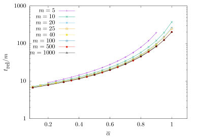
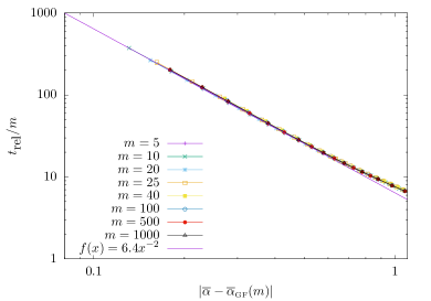
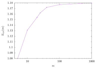
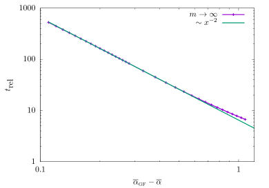
Figure 33: The interpolation transition for pure noise data and a network with second layer weights that do not evolve with time, fixed at $a=1$, see Section G. The noise level is fixed to $\tau=1$ and we considered $h(z)=(3/10)z+z^{2}/2$. Top left panel: relaxation time ((rate for convergence to vanishing error) for different values of $m$. Top right panel: logarithmic plot of the relaxation time. The value of the algorithmic threshold for different values of $m$ is a fitting parameter. Bottom left panel: values of the algorithmic thresholds as a function of $m$. Bottom right panel: the relaxation time as extracted from the scaling limit of the SymmDMFT equations in the $m\to\infty$ limit. The algorithmic threshold is in this case $\overline{\alpha}_{\mbox{\tiny\rm GF}}(\infty)\approx 1.18$ which fits well the behavior plotted in the left bottom plot.

Appendix G Dynamics under mean field initialization for $n/d=\overline{\alpha}$ fixed

G.1 Interpolation threshold at fixed $a(t)=a_{0}$

In this section, we consider an alternative scaling in the large width limit. As before, we use the SymmDMFT equations, and therefore study the limit $n,d\to\infty$ with $n/d\to\overline{\alpha}$. In the previous sections we studied the large width limit $m\to\infty$ with $\alpha=\overline{\alpha}/m$ fixed. In that setting interpolation is only possible when the network complexity scales, i.e. second-layer weights are $a=\Theta(\sqrt{m})$

Here instead we keep $a(t)=1$ and do not let evolve second-layer weights with GF. We consider pure noise data, and show that interpolation takes place if $\overline{\alpha}<\overline{\alpha}_{\mbox{\tiny\rm GF}}(m)$, while the train error remains bounded away from zero for $\overline{\alpha}>\overline{\alpha}_{\mbox{\tiny\rm GF}}(m)$. As expected from Gaussian complexity considerations, the threshold $\overline{\alpha}_{\mbox{\tiny\rm GF}}(m)$ has a finite limit as $m\to\infty$. In particular, for any $\alpha>0$, a network with $a$ bounded cannot interpolate pure noise data.

As thorough in Sec.E we fix $\overline{\alpha}$ and integrate numerically the SymmDMFT equations for finite but increasing values of $m$. We fix the initialization scale $a_{0}$ and the noise level $\tau$ and change only $\overline{\alpha}$.

We observe that for $\overline{\alpha}$ small enough the train error decreases exponentially fast to zero. Namely, recalling that $e_{\mbox{{\rm\footnotesize tr}}}(t;\overline{\alpha}):=\lim_{n,d\to\infty}\widehat{\mathscrsfs{R}}_{n}({\boldsymbol{a}}(t),\boldsymbol{W}(t))$, we have that

$$\overline{\alpha}<\overline{\alpha}_{\mbox{\tiny\rm GF}}(m)\;\;\Rightarrow\;\;e_{\mbox{{\rm\footnotesize tr}}}(t;\overline{\alpha})=\exp\{-t/t^{*}_{\mbox{\rm\tiny rel}}(\overline{\alpha},m)+o(t)\}\,.$$ (G.1)

However, the relaxation time time $t^{*}_{\mbox{\rm\tiny rel}}(\overline{\alpha},m)$ increases as $\overline{\alpha}\uparrow\overline{\alpha}_{\mbox{\tiny\rm GF}}(m)$. Concretely, we define $t_{\mbox{\rm\tiny rel}}(\overline{\alpha},m,c)$ as the infimum time such that $e_{\mbox{{\rm\footnotesize tr}}}(t;\overline{\alpha})\leq c$, where $c$ is some small constant. In practice, we set $c=10^{-7}$. The results are plotted as a function of $\overline{\alpha}$ for several values of $m$ in Fig. 33, top left plot.

For each value of $m$ the relaxation time appears to diverge at the critical point $\overline{\alpha}_{\mbox{\tiny\rm GF}}(m)$ as an inverse power of $\overline{\alpha}_{\mbox{\tiny\rm GF}}(m)-\overline{\alpha}$, namely:

$$\overline{\alpha}\uparrow\overline{\alpha}_{\mbox{\tiny\rm GF}}(m)\;\;\;\Rightarrow\;\;\;t_{\mbox{\rm\tiny rel}}(\overline{\alpha},m,c)=\frac{L(m,c)}{(\overline{\alpha}_{\mbox{\tiny\rm GF}}(m)-\overline{\alpha})^{\nu}}\big{(}1+o(1)\big{)}\,.$$ (G.2)

The exponent $\nu$ appears to be independent of $m$. We fit this form to our data and extract the interpolation thresholds $\overline{\alpha}_{\mbox{\rm\tiny rel}}(m)$. In Fig. 33, top right, we plot $t_{\mbox{\rm\tiny rel}}(\overline{\alpha},m,c)/m$ as a function of the gap to this threshold. This plot confirms the form (G.2), with exponent $\nu\approx 2$. Also, the fact that different curves superimpose indicate that $L(m,c)\approx L_{*}(c)m$.

The estimated interpolation thresholds $\overline{\alpha}_{\mbox{\tiny\rm GF}}(m)$ are plotted as a function of $m$ in the bottom left of Fig. 33. These data are consistent with the existence of a finite limit

$$\overline{\alpha}_{\mbox{\tiny\rm GF}}(\infty)=\lim_{m\to\infty}\overline{\alpha}_{\mbox{\tiny\rm GF}}(m)\,,$$ (G.3)

and numerically $\overline{\alpha}_{\mbox{\tiny\rm GF}}(\infty)\approx 1.18$.

In the next subsection, we derive equations describing the $m\to\infty$ limit for $\overline{\alpha}=O(1)$, $a=O(1)$ fixed. Studying these equations yields further support to Eq. (G.3).

G.2 Infinite width limit at fixed $\overline{\alpha}$

In order to study the limit $m\to\infty$ at fixed $\overline{\alpha}$, we discuss the limit of the SymmDMFT equations when $m\to\infty$. As we have seen previously, the relaxation time of the train error is proportional to $m$. This is clearly visible in Fig. 33-top/left. This suggests that for $m\to\infty$, dynamics takes place on timescales of order $m$. Therefore we propose the following asymptotic ansatz

$$mR_{o}(tm,sm) =\tilde{R}^{\overline{\alpha}}_{o}(t,s)+o_{m}(1)\,, C_{o}(tm,sm) =\tilde{C}^{\overline{\alpha}}_{o}(t,s)+o_{m}(1)\,,$$ (G.4)

$$R_{d}(tm,sm) =\tilde{R}^{\overline{\alpha}}_{d}(t,s)+o_{m}(1)\,, C_{d}(tm,sm) =\tilde{C}^{\overline{\alpha}}_{d}(t,s)+o_{m}(1)\,,$$ (G.5)

$$m\nu(tm) =\tilde{\nu}^{\overline{\alpha}}(t)+o_{m}(1)\,,$$ (G.6)

which defines a set of functions, $\tilde{R}^{\overline{\alpha}}_{d}$, $\tilde{C}^{\overline{\alpha}}_{d}$, $\tilde{R}^{\overline{\alpha}}_{o}$, $\tilde{C}^{\overline{\alpha}}_{o}$ and $\tilde{\nu}^{\overline{\alpha}}$. We now describe the equations that these scaling functions satisfy satisfy. First we define $\tilde{C}_{A}^{\overline{\alpha}}$ and $\tilde{R}_{A}^{\overline{\alpha}}$ as the solution of

$$\begin{split}\delta(t-t^{\prime})&=\int_{t^{\prime}}^{t}\left[\delta(t-s)+\tilde{\Sigma}_{R}(t,s)\right]\tilde{R}^{\overline{\alpha}}_{A}(s,t^{\prime}{\rm d}s\,,)\\ 0&=\int_{0}^{t}\left[\delta(t-s)+\tilde{\Sigma}_{R}(t,s)\right]\tilde{C}^{\overline{\alpha}}_{A}(t^{\prime},s)\,{\rm d}s+\int_{0}^{t^{\prime}}{\rm d}s\tilde{\Sigma}_{C}(t,s)\tilde{R}^{\overline{\alpha}}_{A}(t^{\prime},s)\,{\rm d}s\,,\end{split}$$ (G.7)

where

$$\begin{split}\tilde{\Sigma}_{R}(t,s)&=h^{\prime}(\tilde{C}^{\overline{\alpha}}_{d}(t,s))\tilde{R}^{\overline{\alpha}}_{d}(t,s)+h^{\prime}(\tilde{C}^{\overline{\alpha}}_{o}(t,s))\tilde{R}^{\overline{\alpha}}_{o}(t,s)\\ \tilde{\Sigma}_{C}(t,s)&=\tau^{2}+h(\tilde{C}^{\overline{\alpha}}_{o}(t,s))\,.\end{split}$$ (G.8)

Then we define the limit memory kernels:

$$\begin{split}\tilde{M}_{R}^{(d)}(t,s)&=\overline{\alpha}\tilde{C}_{A}(t,s)h^{\prime\prime}(\tilde{C}^{\overline{\alpha}}_{d}(t,s))\tilde{R}^{\overline{\alpha}}_{d}(t,s)\,,\\ \tilde{M}_{C}^{(d)}(t,s)&=\overline{\alpha}\tilde{C}^{\overline{\alpha}}_{A}(t,s)h^{\prime}(\tilde{C}^{\overline{\alpha}}_{d}(t,s))\,,\\ \tilde{M}_{R}^{(o)}(t,s)&=\overline{\alpha}\left[\tilde{C}_{A}(t,s)h^{\prime\prime}(\tilde{C}^{\overline{\alpha}}_{o}(t,s))\tilde{R}^{\overline{\alpha}}_{o}(t,s)+\tilde{R}^{\overline{\alpha}}_{A}(t,s)h^{\prime}(\tilde{C}^{\overline{\alpha}}_{o}(t,s))\right]\,,\\ \tilde{M}_{C}^{(o)}(t,s)&=\overline{\alpha}\tilde{C}^{\overline{\alpha}}_{A}(t,s)h^{\prime}(\tilde{C}^{\overline{\alpha}}_{o}(t,s))\,.\end{split}$$ (G.9)

Substituting the above ansatz in the SymmDMFT equations and matching the leading order terms, we get the following equations that determine $\tilde{R}^{\overline{\alpha}}_{d}$, $\tilde{C}^{\overline{\alpha}}_{d}$, $\tilde{R}^{\overline{\alpha}}_{o}$, $\tilde{C}^{\overline{\alpha}}_{o}$ and $\tilde{\nu}^{\overline{\alpha}}$:

$$\partial_{t}\tilde{C}^{\overline{\alpha}}_{d}(t,t^{\prime})= -\tilde{\nu}^{\overline{\alpha}}(t)\tilde{C}^{\overline{\alpha}}_{d}(t,t^{\prime})-\int_{0}^{t}\left[\tilde{M}_{R}^{(d)}(t,s)\tilde{C}^{\overline{\alpha}}_{d}(t^{\prime},s)+\tilde{M}_{R}^{(o)}(t,s)\tilde{C}^{\overline{\alpha}}_{o}(t^{\prime},s)\right]\,{\rm d}s$$

$$-\int_{0}^{t^{\prime}}\left[\tilde{M}_{C}^{(d)}(t,s)\tilde{R}^{\overline{\alpha}}_{d}(t^{\prime},s)+\tilde{M}_{C}^{(o)}(t,s)\tilde{R}^{\overline{\alpha}}_{o}(t^{\prime},s)\right]\,{\rm d}s\,,$$ (G.10)

$$\partial_{t}\tilde{C}^{\overline{\alpha}}_{o}(t,t^{\prime})= -\tilde{\nu}^{\overline{\alpha}}(t)\tilde{C}^{\overline{\alpha}}_{o}(t,t^{\prime})-\int_{0}^{t}\left[\tilde{M}_{R}^{(d)}(t,s)+\tilde{M}_{R}^{(o)}(t,s)\right]\tilde{C}^{\overline{\alpha}}_{o}(t^{\prime},s)\,{\rm d}s$$

$$-\int_{0}^{t^{\prime}}\left[\tilde{R}^{\overline{\alpha}}_{o}(t^{\prime},s)+\tilde{R}^{\overline{\alpha}}_{d}(t^{\prime},s)\right]\tilde{M}_{C}^{(o)}(t,s)\,{\rm d}s\,,$$ (G.11)

$$\partial_{t}\tilde{R}^{\overline{\alpha}}_{d}(t,t^{\prime}) =-\tilde{\nu}^{\overline{\alpha}}(t)\tilde{R}^{\overline{\alpha}}_{d}(t,t^{\prime})+\delta(t-t^{\prime})-\int_{t^{\prime}}^{t}{\rm d}s\tilde{M}_{R}^{(d)}(t,s)\tilde{R}^{\overline{\alpha}}_{d}(s,t^{\prime})\,,$$ (G.12)

$$\partial_{t}\tilde{R}^{\overline{\alpha}}_{o}(t,t^{\prime})= -\tilde{\nu}^{\overline{\alpha}}(t)\tilde{R}^{\overline{\alpha}}_{o}(t,t^{\prime})-\int_{t^{\prime}}^{t}\left[\tilde{M}_{R}^{(d)}(t,s)\tilde{R}^{\overline{\alpha}}_{o}(s,t^{\prime})+\tilde{M}_{R}^{(o)}(t,s)\tilde{R}^{\overline{\alpha}}_{d}(s,t^{\prime})\right.$$

$$\left.+\tilde{M}_{R}^{(o)}(t,s)\tilde{R}^{\overline{\alpha}}_{o}(s,t^{\prime})\right]\,{\rm d}s\,,$$ (G.13)

$$\tilde{\nu}^{\overline{\alpha}}(t)= -\int_{0}^{t}{\rm d}s\left[\tilde{M}_{R}^{(d)}(t,s)\tilde{C}_{d}(t,s)+\tilde{M}_{R}^{(o)}(t,s)\tilde{C}^{\overline{\alpha}}_{o}(t,s)\right]\,{\rm d}s$$

$$-\int_{0}^{t}\left[\tilde{M}_{C}^{(d)}(t,s)\tilde{R}^{\overline{\alpha}}_{d}(t,s)+\tilde{M}_{C}^{(o)}(t,s)\tilde{R}^{\overline{\alpha}}_{o}(t,s)\right]\,{\rm d}s\,.$$ (G.14)

These are to be solved with boundary condition

$$\tilde{C}^{\overline{\alpha}}_{o}(0,0) =0\,, \tilde{R}^{\overline{\alpha}}_{o}(0,0) =0\,,$$ (G.15)

$$\tilde{C}^{\overline{\alpha}}_{d}(0,0) =1\,, \tilde{R}^{\overline{\alpha}}_{d}(0^{+},0) =1\>.$$ (G.16)

The scaling behavior of the train error is then given by

$$\lim_{m\to\infty}e_{\mbox{{\rm\footnotesize tr}}}(t)=-\frac{1}{2}\tilde{C}_{A}^{\overline{\alpha}}(t,t)=:e_{\mbox{{\rm\footnotesize tr}}}^{\overline{\alpha}}(t)\,.$$ (G.17)

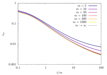
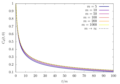
Figure 34: Check of the convergence of the numerical solution of the SymmDMFT for $\overline{\alpha}$ fixed to the scaling solution for $m\to\infty$. The left panel shows the behavior of the train error while the right panel shows the behavior of the correlation $C_{d}(t,0)$. Both panels refer to a model where the teacher is pure noise with $\tau=1$ and the student is made of of neurons whose covariance structure is given by $h(z)=(3/10)z+z^{2}/2$.

In order to test the accuracy of the asymptotic analysis developed in this sections, we solved numerically the SymmDMFT equations for increasing values of $m$ and compare the results to the numerical integration of Eqs. (G.10), (G.14) presented in this section. Some results of this comparison are presented in Fig. 34, which shows good agreement between finite-$m$ curves and $m\to\infty$ limit.

The solution of Eqs. (G.10), (G.14) provides another route to estimate the large-$m$ interpolation threshold $\overline{\alpha}_{\mbox{\tiny\rm GF}}(\infty)$ at fixed $a(t)=1$. Namely, we solve the equations numerically and extract the $t_{\mbox{\rm\tiny rel}}(\overline{\alpha},\infty,c)$, which is defined analogously to above. We then fit the divergence of $t_{\mbox{\rm\tiny rel}}(\overline{\alpha},\infty,c)$ at $\overline{\alpha}_{\mbox{\tiny\rm GF}}(\infty)$ according to Eq. (G.2). We obtain $\overline{\alpha}_{\mbox{\tiny\rm GF}}(\infty)\approx 1.18$, in agreement with the threshold obtained by extrapolating the finite-$m$ thresholds $\overline{\alpha}_{\mbox{\tiny\rm GF}}(m)$. In the bottom right plot of Fig. 33 we plot $t_{\mbox{\rm\tiny rel}}(\overline{\alpha},\infty,c)$ as function of $\overline{\alpha}_{\mbox{\tiny\rm GF}}(\infty)-\overline{\alpha}$. This confirms the behavior of Eq. (G.2) with $\nu\approx 2$.

We conclude by emphasizing that, throughout this section $\alpha(t)=1$ and $\tau=1$ were fixed. If we generalize to arbitrary $\alpha(t)=a_{0}$ and arbitrary $\tau>0$, the threshold $\overline{\alpha}_{\mbox{\tiny\rm GF}}(m)$ will of course on these quantities through the ratio $a_{0}/\tau$.

Appendix H Lower bound on the overfitting timescale

H.1 Proof of Lemma 3.1

By computing the derivative $\partial_{a_{i}}\widehat{\mathscrsfs{R}}({\boldsymbol{a}}(t),\boldsymbol{W}(t))$, we get

$$\frac{{\rm d}\phantom{t}}{{\rm d}t}\big{|}a_{\ell}(t)\big{|} \leq\alpha\cdot\left|\frac{1}{n}\sum_{i=1}^{n}\big{(}y_{i}-f({\boldsymbol{x}}_{i};{\boldsymbol{a}}(t),\boldsymbol{W}(t)\big{)}\sigma({\boldsymbol{w}}_{\ell}(t)^{{\sf T}}{\boldsymbol{x}}_{i})\right|$$

$$\leq\alpha\sqrt{2\widehat{\mathscrsfs{R}}_{n}({\boldsymbol{a}}(t),\boldsymbol{W}(t))}\cdot\sqrt{\frac{1}{n}\sum_{i=1}^{\ell}\sigma({\boldsymbol{w}}_{\ell}^{{\sf T}}{\boldsymbol{x}}_{i})^{2}}$$

$$\leq 4L\alpha\sqrt{2\widehat{\mathscrsfs{R}}_{n}({\boldsymbol{a}}(0),\boldsymbol{W}(0))}\cdot\sqrt{\frac{1}{n}\sum_{i=1}^{\ell}(1+({\boldsymbol{w}}_{\ell}(t)^{{\sf T}}{\boldsymbol{x}}_{i})^{2})}$$

$$\leq 10L\alpha\sqrt{2\widehat{\mathscrsfs{R}}_{n}({\boldsymbol{a}}(0),\boldsymbol{W}(0))}\,,$$

where the last inequality holds with probability at least $1-2\exp(-cn)$ (for some universal $c>0$) by standard upper bounds on the norm of random matrices [Ver18]. Further

$$\sqrt{2n\widehat{\mathscrsfs{R}}_{n}({\boldsymbol{a}}(0),\boldsymbol{W}(0))} =\Big{\|}{\boldsymbol{y}}-\frac{1}{m}\sum_{i=1}^{m}a_{i}\sigma(\boldsymbol{X}{\boldsymbol{w}}_{i})\Big{\|}$$

$$\stackrel{{\scriptstyle(a)}}{{\leq}}\|{\boldsymbol{y}}\|+a_{0}\max_{i\leq m}\big{\|}\sigma(\boldsymbol{X}{\boldsymbol{w}}_{i})\big{\|}$$

$$\stackrel{{\scriptstyle(b)}}{{\leq}}\tau\|{\boldsymbol{g}}\|+\|\varphi(\boldsymbol{X}{\boldsymbol{U}})\|+a_{0}\max_{i\leq m}\big{\|}\sigma(\boldsymbol{X}{\boldsymbol{w}}_{i})\big{\|}$$

$$\leq\tau\|{\boldsymbol{g}}\|+L_{\varphi}\|\boldsymbol{X}{\boldsymbol{U}}\|+a_{0}L\big{\|}\boldsymbol{X}\big{\|}_{\mbox{\tiny\rm op}}+a_{0}\sqrt{n}|\sigma(0)|\,,$$

where in $(a)$ it is understood that $\sigma$ is applied entrywise to $\boldsymbol{X}{\boldsymbol{w}}_{i}i\in{\mathbb{R}}^{n}$ and in $(b)$ we have ${\boldsymbol{g}}\sim{\sf N}({\mathbf{0}},{\boldsymbol{I}}_{n})$ and $\varphi$ is applied row-wise to $\boldsymbol{X}{\boldsymbol{U}}\in{\mathbb{R}}^{n\times k}$. By using standard concentration on the norm of random matrices, with the same probability

$$\sqrt{2\widehat{\mathscrsfs{R}}_{n}({\boldsymbol{a}}(0),\boldsymbol{W}(0))} =C(\tau+a_{0}L)\,.$$

Summarizing the above bounds

$$\frac{{\rm d}\phantom{t}}{{\rm d}t}\big{|}a_{\ell}(t)\big{|} \leq b_{0}\,,$$

which implies the first claim by integration.

To prove the second claim, we consider the following sets of parameters ${\mathcal{W}}_{m,d}^{\infty}({\overline{a}})\subseteq{\mathcal{W}}_{m,d}({\overline{a}})$ (which will also prove useful in the next section)

$${\mathcal{W}}_{m,d}({\overline{a}}) :=\Big{\{}({\boldsymbol{a}},\boldsymbol{W})\in{\mathbb{R}}^{m}\times{\mathbb{R}}^{m\times d}:\;\frac{\|{\boldsymbol{a}}\|_{1}}{m}\leq{\overline{a}},\;\|{\boldsymbol{w}}_{i}\|_{2}=1\;\;\forall i\leq m\Big{\}}\,,$$ (H.1)

$${\mathcal{W}}_{m,d}^{\infty}({\overline{a}}) :=\Big{\{}({\boldsymbol{a}},\boldsymbol{W})\in{\mathbb{R}}^{m}\times{\mathbb{R}}^{m\times d}:\;\|{\boldsymbol{a}}\|_{\infty}\leq{\overline{a}},\;\|{\boldsymbol{w}}_{i}\|_{2}=1\;\;\forall i\leq m\Big{\}}\,.$$ (H.2)

The second claim follows in turn if we prove that

$$\sup_{({\boldsymbol{a}},\boldsymbol{W})\in{\mathcal{W}}_{m,d}({\overline{a}})}\big{|}\widehat{\mathscrsfs{R}}_{n}({\boldsymbol{a}},\boldsymbol{W})-\mathscrsfs{R}({\boldsymbol{a}},\boldsymbol{W})\big{|}\leq C(\alpha,L,\tau)\frac{{\overline{a}}^{2}}{\sqrt{m}}\,.$$ (H.3)

This is a well-known result, that we reproduce for the readers’ convenience. By usual concentration, it is sufficient to bound the expectation. This in turns is bounded by symmetrization and contraction inequality:

$${\mathbb{E}} \sup_{({\boldsymbol{a}},\boldsymbol{W})\in{\mathcal{W}}_{m,d}({\overline{a}})}\big{|}\widehat{\mathscrsfs{R}}_{n}({\boldsymbol{a}},\boldsymbol{W})-\mathscrsfs{R}({\boldsymbol{a}},\boldsymbol{W})\big{|}\leq{\mathbb{E}}\sup_{({\boldsymbol{a}},\boldsymbol{W})\in{\mathcal{W}}_{m,d}({\overline{a}})}\frac{1}{n}\sum_{i=1}^{n}{\varepsilon}_{i}\big{(}y_{i}-f({\boldsymbol{x}}_{i};{\boldsymbol{a}},\boldsymbol{W})\big{)}^{2}$$

$$\leq 2{\mathbb{E}}\sup_{({\boldsymbol{a}},\boldsymbol{W})\in{\mathcal{W}}_{m,d}({\overline{a}})}\frac{1}{n}\sum_{i=1}^{n}{\varepsilon}_{i}y_{i}f({\boldsymbol{x}}_{i};{\boldsymbol{a}},\boldsymbol{W})+{\mathbb{E}}\sup_{({\boldsymbol{a}},\boldsymbol{W})\in{\mathcal{W}}_{m,d}({\overline{a}})}\frac{1}{n}\sum_{i=1}^{n}{\varepsilon}_{i}f({\boldsymbol{x}}_{i};{\boldsymbol{a}},\boldsymbol{W})^{2}$$

$$=:E_{1}+E_{2}\,.$$

We bound term $E_{2}$, since $E_{1}$ follows analogously:

$$E_{1}= {\mathbb{E}}\sup_{({\boldsymbol{a}},\boldsymbol{W})\in{\mathcal{W}}_{m,d}({\overline{a}})}\sum_{i,l=1}^{m}\frac{a_{j}a_{l}}{m^{2}}\frac{1}{n}\sum_{i=1}^{n}{\varepsilon}_{i}\sigma({\boldsymbol{w}}_{j}^{{\sf T}}{\boldsymbol{x}}_{i})\sigma({\boldsymbol{w}}_{l}^{{\sf T}}{\boldsymbol{x}}_{i})$$

$$\leq{\overline{a}}^{2}{\mathbb{E}}\sup_{{\boldsymbol{w}},\tilde{\boldsymbol{w}}\in{\mathbb{S}}^{d-1}}\frac{1}{n}\sum_{i=1}^{n}{\varepsilon}_{i}\sigma({\boldsymbol{w}}^{{\sf T}}{\boldsymbol{x}}_{i})\sigma(\tilde{\boldsymbol{w}}_{l}^{{\sf T}}{\boldsymbol{x}}_{i})$$

$$\leq L^{2}{\overline{a}}^{2}{\mathbb{E}}\sup_{{\boldsymbol{w}}\in{\mathbb{S}}^{d-1}}\frac{1}{n}\sum_{i=1}^{n}{\varepsilon}_{i}{\boldsymbol{w}}^{{\sf T}}{\boldsymbol{x}}_{i}\,,$$

where the last inequality follows by applying the contraction inequality of [Mau16] to $\phi(t_{1},t_{2})=\sigma(t_{1})\sigma(t_{2})$.

H.2 Proof of Proposition 3.2

We also introduce the notations:

$${\boldsymbol{g}}^{{\boldsymbol{w}}}_{n,\ell}({\boldsymbol{a}},\boldsymbol{W}) :=\frac{n}{d|a_{\ell}|}\big{[}\nabla_{{\boldsymbol{w}}_{\ell}}\widehat{\mathscrsfs{R}}_{n}({\boldsymbol{a}},\boldsymbol{W})-\nabla_{{\boldsymbol{w}}_{\ell}}\mathscrsfs{R}({\boldsymbol{a}},\boldsymbol{W})\big{]}\,,$$ (H.4)

$$g^{a}_{n,\ell}({\boldsymbol{a}},\boldsymbol{W}) :=\frac{n}{d}\big{[}\nabla_{a_{\ell}}\widehat{\mathscrsfs{R}}_{n}({\boldsymbol{a}},\boldsymbol{W})-\nabla_{a_{\ell}}\mathscrsfs{R}({\boldsymbol{a}},\boldsymbol{W})\big{]}\,.$$ (H.5)

We begin by establishing a uniform convergence lemma.

Lemma H.1.

Under the data distribution of Section A, assume $\|\varphi\|_{\infty}\leq L$ and the activation function to be bounded differentiable with Lipschitz continuous first derivative $\|\sigma\|_{\infty},\|\sigma^{\prime}\|_{\infty},\|\sigma\|_{\infty}\leq L$. Then there exists a universal constant $C_{1}$, and a constant $c_{0}>0$ dependent on $L,\tau,\alpha$ such that, letting $C_{\alpha}=C_{1}(\alpha\vee 1)$, with probability at least $1-2\exp(-nc_{0})$,

$$\sup_{({\boldsymbol{a}},\boldsymbol{W})\in{\mathcal{W}}_{m,d}({\overline{a}})}\max_{\ell\leq m}\big{\|}{\boldsymbol{g}}^{{\boldsymbol{w}}}_{n,\ell}({\boldsymbol{a}},\boldsymbol{W})\big{\|}\leq C_{\alpha}(L^{2}{\overline{a}}+\tau^{2})\sqrt{\frac{\log(2m)}{m}}\,,$$ (H.6)

$$\sup_{({\boldsymbol{a}},\boldsymbol{W})\in{\mathcal{W}}_{m,d}({\overline{a}})}\max_{\ell\leq m}\big{|}g^{a}_{n,\ell}({\boldsymbol{a}},\boldsymbol{W})\big{|}\leq C_{\alpha}(L^{2}{\overline{a}}+\tau^{2})\frac{1}{\sqrt{m}}\,.$$ (H.7)

Proof.

Gradient with respect to ${\boldsymbol{w}}_{\ell}$. By a concentration argument, it is sufficient to consider the expected supremum. Writing the formula for $\nabla_{{\boldsymbol{w}}_{\ell}}\widehat{\mathscrsfs{R}}_{n}$ and using a standard symmetrization argument, we get

$${\mathbb{E}} \sup_{({\boldsymbol{a}},\boldsymbol{W})\in{\mathcal{W}}_{m,d}({\overline{a}})}\big{\|}{\boldsymbol{g}}^{{\boldsymbol{w}}}_{n,\ell}({\boldsymbol{a}},\boldsymbol{W})\big{\|}={\mathbb{E}}\sup_{({\boldsymbol{a}},\boldsymbol{W})\in{\mathcal{W}}_{m,d}({\overline{a}}),\|{\boldsymbol{u}}\|\leq 1}\langle{\boldsymbol{u}},{\boldsymbol{g}}^{{\boldsymbol{w}}}_{n,\ell}({\boldsymbol{a}},\boldsymbol{W})\rangle$$

$$\leq 2\alpha\,{\mathbb{E}}\sup_{{\boldsymbol{a}},\boldsymbol{W},{\boldsymbol{u}}}\frac{1}{n}\sum_{i=1}^{n}{\varepsilon}_{i}y_{i}\sigma^{\prime}({\boldsymbol{w}}_{\ell}^{{\sf T}}{\boldsymbol{x}}_{i}){\boldsymbol{u}}^{{\sf T}}{\boldsymbol{x}}_{i}+2\alpha\,{\mathbb{E}}\sup_{{\boldsymbol{a}},\boldsymbol{W},{\boldsymbol{u}}}\frac{1}{n}\sum_{i=1}^{n}{\varepsilon}_{i}\sum_{j=1}^{m}\frac{a_{j}}{m}\sigma({\boldsymbol{w}}_{j}^{{\sf T}}{\boldsymbol{x}}_{i})\sigma^{\prime}({\boldsymbol{w}}_{\ell}^{{\sf T}}{\boldsymbol{x}}_{i}){\boldsymbol{u}}^{{\sf T}}{\boldsymbol{x}}_{i}$$

$$=:B_{1}+B_{2}\,,$$

where the ${\varepsilon}_{i}$ are i.i.d. Radamacher random variables and in the last two lines it is understood that the supremum is over $({\boldsymbol{a}},\boldsymbol{W})\in{\mathcal{W}}_{m,d}({\overline{a}}),\|{\boldsymbol{u}}\|\leq 1$. Consider the second term in the last expression:

$$B_{2} =2\alpha{\overline{a}}\,{\mathbb{E}}\sup_{\boldsymbol{W},{\boldsymbol{u}}}\max_{j\leq m}\frac{1}{n}\sum_{i=1}^{n}{\varepsilon}_{i}\sigma({\boldsymbol{w}}_{j}^{{\sf T}}{\boldsymbol{x}}_{i})\sigma^{\prime}({\boldsymbol{w}}_{\ell}^{{\sf T}}{\boldsymbol{x}}_{i}){\boldsymbol{u}}^{{\sf T}}{\boldsymbol{x}}_{i}$$

$$\leq 2\alpha{\overline{a}}\,{\mathbb{E}}\sup_{{\boldsymbol{w}},\overline{\boldsymbol{w}},{\boldsymbol{u}}\in{\sf B}^{d}(1)}\frac{1}{n}\sum_{i=1}^{n}{\varepsilon}_{i}\sigma({\boldsymbol{w}}^{{\sf T}}{\boldsymbol{x}}_{i})\sigma^{\prime}(\overline{\boldsymbol{w}}^{{\sf T}}{\boldsymbol{x}}_{i}){\boldsymbol{u}}^{{\sf T}}{\boldsymbol{x}}_{i}$$

$$\leq 2\alpha{\overline{a}}\,{\mathbb{E}}\sup_{{\boldsymbol{w}},\overline{\boldsymbol{w}},{\boldsymbol{u}}\in{\sf B}^{d}(1)}\frac{1}{n}\sum_{i=1}^{n}{\varepsilon}_{i}\sigma({\boldsymbol{w}}^{{\sf T}}{\boldsymbol{x}}_{i})\sigma^{\prime}(\overline{\boldsymbol{w}}^{{\sf T}}{\boldsymbol{x}}_{i})\eta({\boldsymbol{u}}^{{\sf T}}{\boldsymbol{x}}_{i})$$

$$\phantom{AAAAA}+2\alpha{\overline{a}}\,{\mathbb{E}}\sup_{{\boldsymbol{w}},\overline{\boldsymbol{w}},{\boldsymbol{u}}\in{\sf B}^{d}(1)}\frac{1}{n}\sum_{i=1}^{n}{\varepsilon}_{i}\sigma({\boldsymbol{w}}^{{\sf T}}{\boldsymbol{x}}_{i})\sigma^{\prime}(\overline{\boldsymbol{w}}^{{\sf T}}{\boldsymbol{x}}_{i})\overline{\eta}({\boldsymbol{u}}^{{\sf T}}{\boldsymbol{x}}_{i})$$

$$=:B_{2,1}+B_{2,2}\,,$$

where $\eta(x)=x{\boldsymbol{1}}_{|x|\leq M}+M({\boldsymbol{1}}_{x>M}-{\boldsymbol{1}}_{x<-M})$, and $\overline{\eta}(x)=x-\eta(x)$. Defining $\phi(t_{1},t_{2},t_{3}):=\sigma(t_{1})\sigma^{\prime}(t_{2})\eta(t_{3})$ (which is $CL^{2}M$-Lipschitz for $M\geq 1$) and using a generalization of Talagrand’s contraction inequality [Mau16],

$$B_{2,1} \leq CL^{2}M\alpha{\overline{a}}\left\{{\mathbb{E}}\sup_{{\boldsymbol{w}}\in{\sf B}^{d}(1)}\frac{1}{n}\sum_{i=1}^{n}{\varepsilon}_{i}{\boldsymbol{w}}^{{\sf T}}{\boldsymbol{x}}_{i}+{\mathbb{E}}\sup_{\overline{\boldsymbol{w}}\in{\sf B}^{d}(1)}\frac{1}{n}\sum_{i=1}^{n}{\varepsilon}_{i}\overline{\boldsymbol{w}}^{{\sf T}}{\boldsymbol{x}}_{i}+{\mathbb{E}}\sup_{{\boldsymbol{u}}\in{\sf B}^{d}(1)}\frac{1}{n}\sum_{i=1}^{n}{\varepsilon}_{i}{\boldsymbol{u}}^{{\sf T}}{\boldsymbol{x}}_{i}\right\}$$

$$\leq CL^{2}M\alpha{\overline{a}}\sqrt{\frac{d}{n}}$$

$$\leq C_{\alpha}L^{2}{\overline{a}}\frac{M}{\sqrt{m}}\,.$$

Next consider $B_{2,2}$:

$$B_{2,2} \leq 2\alpha{\overline{a}}L^{2}{\mathbb{E}}\sup_{{\boldsymbol{u}}\in{\sf B}^{d}(1)}\frac{1}{n}\sum_{i=1}^{n}|\overline{\eta}({\boldsymbol{u}}^{{\sf T}}{\boldsymbol{x}}_{i})|$$

$$\leq 2\alpha{\overline{a}}L^{2}\sup_{{\boldsymbol{u}}\in{\sf B}^{d}(1)}{\mathbb{E}}|\overline{\eta}({\boldsymbol{u}}^{{\sf T}}{\boldsymbol{x}}_{i})|+2\alpha{\overline{a}}L^{2}{\mathbb{E}}\sup_{{\boldsymbol{u}}\in{\sf B}^{d}(1)}\frac{1}{n}\sum_{i=1}^{n}{\varepsilon}_{i}|\overline{\eta}({\boldsymbol{u}}^{{\sf T}}{\boldsymbol{x}}_{i})|$$

$$\leq C_{\alpha}L^{2}{\overline{a}}e^{-M^{2}/4}+C_{\alpha}L^{2}{\overline{a}}\sqrt{\frac{d}{n}}\,,$$

where the last inequality holds because ${\boldsymbol{u}}^{{\sf T}}{\boldsymbol{x}}_{i}$ is Gaussian with variance $\|{\boldsymbol{u}}\|^{2}$, and using again the contraction inequality. Collecting various terms and optimizing over $M\geq 1$, we obtain

$$B_{2} \leq C_{\alpha}L^{2}{\overline{a}}\Big{\{}\frac{M}{\sqrt{m}}+e^{-M^{2}/4}\Big{\}}$$

$$\leq C_{\alpha}L^{2}{\overline{a}}\sqrt{\frac{\log m\vee 1}{m}}\,.$$

The proof of Eq. (H.6) is completed by bounding $B_{1}$ along the same lines.

Gradient with respect to $a_{\ell}$. Writing $\nabla_{a_{\ell}}\widehat{\mathscrsfs{R}}_{n}$ and using symmetrization, we get

$${\mathbb{E}} \sup_{({\boldsymbol{a}},\boldsymbol{W})\in{\mathcal{W}}_{m,d}({\overline{a}})}\big{|}g^{a}_{n,\ell}({\boldsymbol{a}},\boldsymbol{W})\big{|}={\mathbb{E}}\sup_{({\boldsymbol{a}},\boldsymbol{W})\in{\mathcal{W}}_{m,d}({\overline{a}}),\|{\boldsymbol{u}}\|\leq 1}g^{a}_{n,\ell}({\boldsymbol{a}},\boldsymbol{W})$$

$$\leq 2\alpha\,{\mathbb{E}}\sup_{\boldsymbol{W},{\boldsymbol{u}}}\frac{1}{n}\sum_{i=1}^{n}{\varepsilon}_{i}y_{i}\sigma({\boldsymbol{w}}_{\ell}^{{\sf T}}{\boldsymbol{x}}_{i})+2\alpha\,{\mathbb{E}}\sup_{{\boldsymbol{a}},\boldsymbol{W},{\boldsymbol{u}}}\frac{1}{n}\sum_{i=1}^{n}{\varepsilon}_{i}\sum_{j=1}^{m}\frac{a_{j}}{m}\sigma({\boldsymbol{w}}_{j}^{{\sf T}}{\boldsymbol{x}}_{i})\sigma({\boldsymbol{w}}_{\ell}^{{\sf T}}{\boldsymbol{x}}_{i})$$

$$=:D_{1}+D_{2}\,.$$

Consider term $D_{2}$, and define the $L^{2}$-Lipschitz function $\psi(t_{1},t_{2}):=\sigma(t_{1})\sigma(t_{2})$,

$$D_{2} \leq 2\alpha{\overline{a}}\,{\mathbb{E}}\sup_{\boldsymbol{W},{\boldsymbol{u}}}\max_{j\leq m}\frac{1}{n}\sum_{i=1}^{n}{\varepsilon}_{i}\sigma({\boldsymbol{w}}_{j}^{{\sf T}}{\boldsymbol{x}}_{i})\sigma({\boldsymbol{w}}_{\ell}^{{\sf T}}{\boldsymbol{x}}_{i})$$

$$\leq 2\alpha{\overline{a}}\,{\mathbb{E}}\sup_{{\boldsymbol{w}},\overline{\boldsymbol{w}}\in{\sf B}^{d}(1)}\frac{1}{n}\sum_{i=1}^{n}{\varepsilon}_{i}\psi({\boldsymbol{w}}^{{\sf T}}{\boldsymbol{x}}_{i},{\boldsymbol{w}}^{{\sf T}}{\boldsymbol{x}}_{i})$$

$$\leq CL^{2}{\overline{a}}\alpha\sqrt{\frac{d}{n}}\leq C_{\alpha}L^{2}{\overline{a}}\frac{1}{\sqrt{m}}\,.$$

Term $D_{1}$ is controlled analogously, yielding the proof of Eq. (H.7). ∎

We next prove some continuity properties of the population risk $\mathscrsfs{R}$. It is useful to recall the form:

$$\mathscrsfs{R}({\boldsymbol{a}},\boldsymbol{W})=\frac{1}{2}(\tau^{2}+\|\varphi\|^{2})-\frac{1}{m}\sum_{i=1}^{m}a_{i}\widehat{\varphi}({\boldsymbol{U}}^{{\sf T}}{\boldsymbol{w}}_{i})+\frac{1}{2m^{2}}\sum_{i,j=1}^{m}a_{i}a_{j}h({\boldsymbol{w}}_{i}^{{\sf T}}{\boldsymbol{w}}_{j})\,.$$ (H.8)

Lemma H.2.

Under the data distribution of Section A, assume $\|\varphi\|_{\infty}\leq L$ and the activation function to be bounded differentiable with Lipschitz continuous first derivative $\|\sigma\|_{\infty},\|\sigma^{\prime}\|_{\infty},\|\sigma\|_{\infty}\leq L$. Then, there exists an absolute constant $C$ such that for any $({\boldsymbol{a}},\boldsymbol{W}),({\boldsymbol{a}},\tilde{\boldsymbol{W}})\in{\mathcal{W}}_{m,d}({\overline{a}})$:

$$\big{\|}\nabla_{{\boldsymbol{w}}_{\ell}}\mathscrsfs{R}({\boldsymbol{a}},\tilde{\boldsymbol{W}})-\nabla_{{\boldsymbol{w}}_{\ell}}\mathscrsfs{R}({\boldsymbol{a}},\boldsymbol{W})\big{\|} \leq CL^{2}\,\frac{|a_{\ell}|}{m}\,(1+{\overline{a}})\max_{j\leq m}\big{\|}\tilde{\boldsymbol{w}}_{j}-{\boldsymbol{w}}_{j}\big{\|}\,,$$ (H.9)

$$\big{|}\partial_{a_{\ell}}\mathscrsfs{R}({\boldsymbol{a}},\tilde{\boldsymbol{W}})-\partial_{a_{\ell}}\mathscrsfs{R}({\boldsymbol{a}},\boldsymbol{W})\big{|} \leq\frac{CL^{2}}{m}\,(1+{\overline{a}})\max_{j\leq m}\big{\|}\tilde{\boldsymbol{w}}_{j}-{\boldsymbol{w}}_{j}\big{\|}\,,$$ (H.10)

and

$$\big{\|}\nabla_{{\boldsymbol{w}}_{\ell}}\mathscrsfs{R}({\boldsymbol{\tilde{a}}},\boldsymbol{W})-\nabla_{{\boldsymbol{w}}_{\ell}}\mathscrsfs{R}({\boldsymbol{a}},\boldsymbol{W})\big{\|} \leq\frac{CL}{m}(1+{\overline{a}})|\tilde{a}_{\ell}-a_{\ell}|+CL\frac{|a_{\ell}|}{m^{2}}\|{\boldsymbol{\tilde{a}}}-{\boldsymbol{a}}\|_{1}\,,$$ (H.11)

$$\big{|}\partial_{a_{\ell}}\mathscrsfs{R}({\boldsymbol{\tilde{a}}},\tilde{\boldsymbol{W}})-\partial_{a_{\ell}}\mathscrsfs{R}({\boldsymbol{a}},\boldsymbol{W})\big{|} \leq\frac{CL}{m^{2}}\,\big{\|}{\boldsymbol{\tilde{a}}}-{\boldsymbol{a}}\big{\|}_{1}\,.$$ (H.12)

Proof.

Proof of Eq. (H.9). Differentiating Eq. (H.8)

$$\frac{m}{a_{\ell}}\nabla_{{\boldsymbol{w}}_{\ell}}\mathscrsfs{R}({\boldsymbol{a}},\boldsymbol{W})=-{\boldsymbol{U}}\nabla\widehat{\varphi}({\boldsymbol{U}}^{{\sf T}}{\boldsymbol{w}}_{\ell})+\sum_{j=1}^{m}\frac{a_{j}}{m}h^{\prime}_{s}({\boldsymbol{w}}_{\ell}^{\sf T}{\boldsymbol{w}}_{j}){\boldsymbol{w}}_{j}\,.$$ (H.13)

Therefore

$$\frac{m}{|a_{\ell}|}\big{\|}\nabla_{{\boldsymbol{w}}_{\ell}}\mathscrsfs{R}({\boldsymbol{a}},\tilde{\boldsymbol{W}})-\nabla_{{\boldsymbol{w}}_{\ell}}\mathscrsfs{R}({\boldsymbol{a}},\boldsymbol{W})\big{\|}\leq \big{\|}\nabla\widehat{\varphi}({\boldsymbol{U}}^{{\sf T}}\tilde{\boldsymbol{w}}_{\ell})-\nabla\widehat{\varphi}({\boldsymbol{U}}^{{\sf T}}{\boldsymbol{w}}_{\ell})\|$$

$$+\sum_{j=1}^{m}\frac{|a_{j}|}{m}\big{\|}h^{\prime}_{s}(\tilde{\boldsymbol{w}}_{\ell}^{\sf T}\tilde{\boldsymbol{w}}_{j})\tilde{\boldsymbol{w}}_{j}-h^{\prime}_{s}({\boldsymbol{w}}_{\ell}^{\sf T}{\boldsymbol{w}}_{j}){\boldsymbol{w}}_{j}\big{\|}$$

$$\leq CL^{2}\|\tilde{\boldsymbol{w}}_{\ell}-{\boldsymbol{w}}_{\ell}\|+{\overline{a}}\max_{j\leq m}\big{\|}h^{\prime}_{s}(\tilde{\boldsymbol{w}}_{\ell}^{\sf T}\tilde{\boldsymbol{w}}_{j})\tilde{\boldsymbol{w}}_{j}-h^{\prime}_{s}({\boldsymbol{w}}_{\ell}^{\sf T}{\boldsymbol{w}}_{j}){\boldsymbol{w}}_{j}\big{\|}\,.$$

The assumptions on $\sigma$ imply that $\|h^{\prime}\|_{\mbox{\tiny\rm Lip}}\leq L^{2}$, whence

$$\big{\|}h^{\prime}_{s}(\tilde{\boldsymbol{w}}_{\ell}^{\sf T}\tilde{\boldsymbol{w}}_{j})\tilde{\boldsymbol{w}}_{j}-h^{\prime}_{s}({\boldsymbol{w}}_{\ell}^{\sf T}{\boldsymbol{w}}_{j}){\boldsymbol{w}}_{j}\big{\|}\leq CL^{2}\|\tilde{\boldsymbol{w}}_{j}-{\boldsymbol{w}}_{j}\|+CL^{2}\|\tilde{\boldsymbol{w}}_{\ell}-{\boldsymbol{w}}_{\ell}\|\,.$$

Substituting above, this yields the claim (H.9).

Proof of Eq. (H.10). We proceed analogously to the previous point. Namely

$$m\partial_{a_{\ell}}\mathscrsfs{R}({\boldsymbol{a}},\boldsymbol{W})=-\widehat{\varphi}({\boldsymbol{U}}^{{\sf T}}{\boldsymbol{w}}_{\ell})+\sum_{j=1}^{m}\frac{a_{j}}{m}h({\boldsymbol{w}}_{\ell}^{\sf T}{\boldsymbol{w}}_{j})\,,$$ (H.14)

whence

$$m\big{|}\partial_{a_{\ell}}\mathscrsfs{R}({\boldsymbol{a}},\tilde{\boldsymbol{W}})-\partial_{a_{\ell}}\mathscrsfs{R}({\boldsymbol{a}},\boldsymbol{W})\big{|} \leq\big{|}\widehat{\varphi}({\boldsymbol{U}}^{{\sf T}}\tilde{\boldsymbol{w}}_{\ell})-\widehat{\varphi}({\boldsymbol{U}}^{{\sf T}}{\boldsymbol{w}}_{\ell})\big{|}+\sum_{j=1}^{m}\frac{|a_{j}|}{m}\big{|}h(\tilde{\boldsymbol{w}}_{\ell}^{\sf T}\tilde{\boldsymbol{w}}_{j})-h({\boldsymbol{w}}_{\ell}^{\sf T}{\boldsymbol{w}}_{j})\big{|}$$

$$\leq CL^{2}\|\tilde{\boldsymbol{w}}_{\ell}-{\boldsymbol{w}}_{\ell}\|+C{\overline{a}}L^{2}\big{(}\|\tilde{\boldsymbol{w}}_{\ell}-{\boldsymbol{w}}_{\ell}\|+\|\tilde{\boldsymbol{w}}_{j}-{\boldsymbol{w}}_{j}\|\big{)}\,,$$

which implies immediately Eq. (H.10)

Proof of Eq. (H.11). Recalling Eq. (H.13), we have

$$m\big{\|}\nabla_{{\boldsymbol{w}}_{\ell}}\mathscrsfs{R}({\boldsymbol{\tilde{a}}},\boldsymbol{W})-\nabla_{{\boldsymbol{w}}_{\ell}}\mathscrsfs{R}({\boldsymbol{a}},\boldsymbol{W})\big{\|}\leq \big{\|}\nabla\widehat{\varphi}({\boldsymbol{U}}^{{\sf T}}{\boldsymbol{w}}_{\ell})\|\,|\tilde{a}_{\ell}-a_{\ell}|+\sum_{j=1}^{m}\frac{1}{m}\big{\|}h^{\prime}_{s}({\boldsymbol{w}}_{\ell}^{\sf T}{\boldsymbol{w}}_{j}){\boldsymbol{w}}_{j}\big{\|}\,|\tilde{a}_{\ell}\tilde{a}_{j}-a_{\ell}a_{j}|$$

$$\leq CL|\tilde{a}_{\ell}-a_{\ell}|+CL\frac{|a_{\ell}|}{m}\|{\boldsymbol{\tilde{a}}}-{\boldsymbol{a}}\|_{1}+CL{\overline{a}}\,|\tilde{a}_{\ell}-a_{\ell}|\,,$$

which proves the desired claim.

Proof of Eq. (H.11). Recalling Eq. (H.13), we have

$$m\big{|}\partial_{a_{\ell}}\mathscrsfs{R}({\boldsymbol{\tilde{a}}},\boldsymbol{W})-\partial_{a_{\ell}}\mathscrsfs{R}({\boldsymbol{a}},\boldsymbol{W})\big{|} \leq\sum_{j=1}^{m}\frac{1}{m}|h({\boldsymbol{w}}_{\ell}^{\sf T}{\boldsymbol{w}}_{j})|\cdot|\tilde{a}_{j}-a_{j}|$$

$$\leq\frac{CL}{m}\|{\boldsymbol{\tilde{a}}}-{\boldsymbol{a}}\|_{1}$$

∎

Using the last lemma and triangle inequality we get the following.

Corollary H.3.

Under the assumptions of Lemma H.2, we have, for all $({\boldsymbol{a}},\boldsymbol{W}),({\boldsymbol{a}},\tilde{\boldsymbol{W}})\in{\mathcal{W}}_{m,d}^{\infty}({\overline{a}})$:

$$\max_{\ell\leq m}\big{\|}\nabla_{{\boldsymbol{w}}_{\ell}}\mathscrsfs{R}({\boldsymbol{\tilde{a}}},\tilde{\boldsymbol{W}})-\nabla_{{\boldsymbol{w}}_{\ell}}\mathscrsfs{R}({\boldsymbol{a}},\boldsymbol{W})\big{\|} \leq\frac{C_{L}{\overline{a}}}{m}(1+{\overline{a}})\max_{j\leq m}\|\tilde{\boldsymbol{w}}_{j}-{\boldsymbol{w}}_{j}\|+\frac{C_{L}}{m}(1+{\overline{a}})\|{\boldsymbol{\tilde{a}}}-{\boldsymbol{a}}\|_{\infty}\,,$$ (H.15)

$$\max_{\ell\leq m}\big{|}\partial_{a_{\ell}}\mathscrsfs{R}({\boldsymbol{\tilde{a}}},\tilde{\boldsymbol{W}})-\partial_{a_{\ell}}\mathscrsfs{R}({\boldsymbol{a}},\boldsymbol{W})\big{|} \leq\frac{C_{L}}{m}(1+{\overline{a}})\max_{j\leq m}\|\tilde{\boldsymbol{w}}_{j}-{\boldsymbol{w}}_{j}\|+\frac{C_{L}}{m}\|{\boldsymbol{\tilde{a}}}-{\boldsymbol{a}}\|_{\infty}\,.$$ (H.16)

We next consider ${\boldsymbol{a}}(t),\boldsymbol{W}(t)$ that follows GF with respect to the empirical risk, as per Eq. (A.10), which we rewrite as

$$\begin{split}\dot{{\boldsymbol{a}}}(t)&=-\frac{n}{d}\nabla_{{\boldsymbol{a}}}\mathscrsfs{R}({\boldsymbol{a}}(t),\boldsymbol{W}(t))\,,\\ \dot{{\boldsymbol{w}}}_{i}(t)&=-\frac{n}{d}{\boldsymbol{P}}^{\perp}_{{\boldsymbol{w}}_{i}}\nabla_{{\boldsymbol{w}}_{i}}\mathscrsfs{R}({\boldsymbol{a}}(t),\boldsymbol{W}(t))\;\;\;\;\forall i=1,\ldots,m\,,\end{split}$$ (H.17)

and denote by ${\boldsymbol{a}}_{0}(t),\boldsymbol{W}_{0}(t)$ the GF with respect to population risk:

$$\begin{split}\dot{{\boldsymbol{a}}}_{0}(t)&=-\frac{n}{d}\nabla_{{\boldsymbol{a}}}\mathscrsfs{R}({\boldsymbol{a}}_{0}(t),\boldsymbol{W}_{0}(t))\,,\\ \dot{{\boldsymbol{w}}}_{0,i}(t)&=-\frac{n}{d}{\boldsymbol{P}}^{\perp}_{{\boldsymbol{w}}_{i}}\nabla_{{\boldsymbol{w}}_{i}}\mathscrsfs{R}({\boldsymbol{a}}_{0}(t),\boldsymbol{W}_{0}(t))\;\;\;\;\forall i=1,\ldots,m\,.\end{split}$$ (H.18)

Lemma H.4.

Under the data distribution of Section A, assume $\|\varphi\|_{\infty}\leq L$ and the activation function to be bounded differentiable with Lipschitz continuous first derivative $\|\sigma\|_{\infty},\|\sigma^{\prime}\|_{\infty},\|\sigma\|_{\infty}\leq L$. Let $({\boldsymbol{a}}(t),\boldsymbol{W}(t))$, $({\boldsymbol{a}}_{0}(t),\boldsymbol{W}_{0}(t))$, be defined as above, with $\boldsymbol{W}(0)=\boldsymbol{W}_{0}(0)$ and ${\boldsymbol{a}}(0)={\boldsymbol{a}}_{0}(0)$ such that $\|{\boldsymbol{a}}(0)\|_{1}/m\leq a_{0}$. Define

$$T_{*}(m;c):=\inf\Big{\{}t:\,\big{(}\|{\boldsymbol{a}}(t)\|_{\infty}\vee\|{\boldsymbol{a}}_{0}(t)\|_{\infty}\big{)}\geq(c\log m)^{1/3}\Big{\}}\wedge(c\log m)^{1/3}\,.$$ (H.19)

Then there exist positive constants $c_{1}=c_{1}(L)$, $c_{0}=c_{0}(L,\alpha,\tau)$, $C=C(\alpha)$ such that, with probability at least $1-2\exp(-c_{0}n)$,

$$\sup_{t\leq T_{*}(m;c_{1})}\Delta(t)\leq\frac{C}{m^{1/4}}\,,\;\;\;\Delta(t):=\max_{\ell\leq m}\|\tilde{\boldsymbol{w}}_{\ell}(t)-{\boldsymbol{w}}_{\ell}(t)\|+\|{\boldsymbol{\tilde{a}}}(t)-{\boldsymbol{a}}(t)\|_{\infty}\,.$$ (H.20)

Proof.

We will prove that the desired bound holds on the high-probability event of Lemma H.1, where by we set ${\overline{a}}=(c_{1}\log m)^{1/4}$. Throughout the proof, we use $c_{0}$, $c_{1}$, $C$ to denote constants that might change from line to line, with dependence on the parameters of the problem as per the statement of the lemma.

We start by noting that, letting ${\boldsymbol{v}}_{i}=-(n/d)\nabla_{{\boldsymbol{w}}_{i}}\widehat{\mathscrsfs{R}}_{n}({\boldsymbol{a}},\boldsymbol{W})$ and ${\boldsymbol{v}}_{0,i}=-(n/d)\nabla_{{\boldsymbol{w}}_{0,i}}\mathscrsfs{R}({\boldsymbol{a}}_{0},\boldsymbol{W}_{0}$, and ${\boldsymbol{P}}_{{\boldsymbol{w}}}^{\perp}:={\boldsymbol{I}}-{\boldsymbol{w}}{\boldsymbol{w}}^{{\sf T}}$ the projector orthogonal to ${\boldsymbol{w}}$.

$$\big{\|}{\boldsymbol{P}}^{\perp}_{{\boldsymbol{w}}_{i}}{\boldsymbol{v}}_{i}-{\boldsymbol{P}}^{\perp}_{{\boldsymbol{w}}_{0,i}}{\boldsymbol{v}}_{0,i}\big{\|} \leq\big{\|}{\boldsymbol{P}}^{\perp}_{{\boldsymbol{w}}_{i}}({\boldsymbol{v}}_{i}-{\boldsymbol{v}}_{0,i})\big{\|}+\big{\|}({\boldsymbol{P}}^{\perp}_{{\boldsymbol{w}}_{i}}-{\boldsymbol{P}}^{\perp}_{{\boldsymbol{w}}_{0,i}}){\boldsymbol{v}}_{0,i}\|$$

$$\leq\|{\boldsymbol{v}}_{i}-{\boldsymbol{v}}_{0,i}\|+\|{\boldsymbol{w}}_{i}{\boldsymbol{w}}_{i}^{{\sf T}}-{\boldsymbol{w}}_{0,i}{\boldsymbol{w}}_{0,i}^{{\sf T}}\|_{\mbox{\tiny\rm op}}\|{\boldsymbol{v}}_{0,i}\|$$

$$\leq\|{\boldsymbol{v}}_{i}-{\boldsymbol{v}}_{0,i}\|+2\|{\boldsymbol{w}}_{i}-{\boldsymbol{w}}_{0,i}\|_{\mbox{\tiny\rm op}}\|{\boldsymbol{v}}_{0,i}\|\,.$$

Hence, comparing the evolution of ${\boldsymbol{w}}_{i}(t)$ and ${\boldsymbol{w}}_{0,i}(t)$, we get

$$\frac{{\rm d}\phantom{t}}{{\rm d}t}\|{\boldsymbol{w}}_{i}(t)-{\boldsymbol{w}}_{0,i}(t)\|\leq \;\frac{n}{d}\big{\|}\nabla_{{\boldsymbol{w}}_{i}}\widehat{\mathscrsfs{R}}_{n}({\boldsymbol{a}}(t),\boldsymbol{W}(t))-\nabla_{{\boldsymbol{w}}_{i}}\mathscrsfs{R}({\boldsymbol{a}}_{0}(t),\boldsymbol{W}_{0}(t))\big{\|}$$

$$+\frac{n}{d}\|\nabla_{{\boldsymbol{w}}_{i}}\mathscrsfs{R}({\boldsymbol{a}}_{0}(t),\boldsymbol{W}_{0}(t)))\|\cdot\|{\boldsymbol{w}}_{i}(t)-{\boldsymbol{w}}_{i,0}(t)\|$$

$$=: \;D_{1}+D_{2}\cdot\|{\boldsymbol{w}}_{i}(t)-{\boldsymbol{w}}_{i,0}(t)\|\,.$$

Since we are working on the event of Lemma H.1, and using Corollary H.3, we get, for $t\leq T_{*}(m;c)$.

$$D_{1}\leq \;\frac{n}{d}\big{\|}\nabla_{{\boldsymbol{w}}_{i}}\widehat{\mathscrsfs{R}}_{n}({\boldsymbol{a}}(t),\boldsymbol{W}(t))-\nabla_{{\boldsymbol{w}}_{i}}\mathscrsfs{R}({\boldsymbol{a}}(t),\boldsymbol{W}(t))\big{\|}$$

$$\phantom{AAAAA}+\frac{n}{d}\big{\|}\nabla_{{\boldsymbol{w}}_{i}}\mathscrsfs{R}({\boldsymbol{a}}(t),\boldsymbol{W}(t))-\nabla_{{\boldsymbol{w}}_{i}}\mathscrsfs{R}({\boldsymbol{a}}_{0}(t),\boldsymbol{W}_{0}(t))\big{\|}$$

$$\leq \;C(L^{2}{\overline{a}}+\tau^{2})\sqrt{\frac{\log(2m)}{m}}+C_{L}\alpha(1+{\overline{a}}^{2})\max_{j\leq m}\|{\boldsymbol{w}}_{j}(t)-{\boldsymbol{w}}_{0,j}(t)\|$$

$$\phantom{AAAAA}+C_{L}\alpha(1+{\overline{a}})\|{\boldsymbol{a}}(t)-{\boldsymbol{a}}_{0}(t)\|_{\infty}\,.$$

Further

$$D_{2} =\alpha|a_{i}|\Big{\|}{\boldsymbol{U}}\nabla\widehat{\varphi}({\boldsymbol{U}}^{{\sf T}}{\boldsymbol{w}}_{i})-\frac{1}{m}\sum_{j=1}^{m}a_{j}h^{\prime}_{s}({\boldsymbol{w}}_{i}^{{\sf T}}{\boldsymbol{w}}_{j}){\boldsymbol{w}}_{j}\Big{\|}$$

$$\leq C\alpha{\overline{a}}\big{(}L+{\overline{a}}L^{2}\big{)}\,.$$

Collecting all the terms, we get

$$\frac{{\rm d}\phantom{t}}{{\rm d}t}\|{\boldsymbol{w}}_{i}(t)-{\boldsymbol{w}}_{0,i}(t)\|\leq C(L^{2}{\overline{a}}+\tau^{2})\sqrt{\frac{\log(2m)}{m}}+C_{L}\alpha(1+{\overline{a}}^{2})\Delta(t)\,.$$ (H.21)

We next consider the evolution of second-layer weights:

$$\frac{{\rm d}\phantom{t}}{{\rm d}t}|a_{i}(t)-a_{0,i}(t)\|\leq \;\frac{n}{d}\big{\|}\partial_{a_{i}}\widehat{\mathscrsfs{R}}_{n}({\boldsymbol{a}}(t),\boldsymbol{W}(t))-\partial_{a_{i}}\mathscrsfs{R}({\boldsymbol{a}}_{0}(t),\boldsymbol{W}_{0}(t))\big{\|}$$

$$\leq \;\frac{n}{d}\big{\|}\partial_{a_{i}}\widehat{\mathscrsfs{R}}_{n}({\boldsymbol{a}}(t),\boldsymbol{W}(t))-\partial_{a_{i}}\mathscrsfs{R}({\boldsymbol{a}}(t),\boldsymbol{W}(t))\big{\|}$$

$$\;\;\;\;\;\;\;+\frac{n}{d}\big{\|}\partial_{a_{i}}\mathscrsfs{R}_{n}({\boldsymbol{a}}(t),\boldsymbol{W}(t))-\partial_{a_{i}}\mathscrsfs{R}({\boldsymbol{a}}_{0}(t),\boldsymbol{W}_{0}(t))\big{\|}$$

$$\leq C(L^{2}{\overline{a}}+\tau^{2})\frac{1}{\sqrt{m}}+C_{L}\alpha(1+{\overline{a}})\max_{j\leq m}\|{\boldsymbol{w}}_{j}(t)-{\boldsymbol{w}}_{0,j}(t)\|+C_{L}\alpha\|{\boldsymbol{a}}(t)-{\boldsymbol{a}}_{0}(t)\|_{\infty}$$

$$\leq \;C(L^{2}{\overline{a}}+\tau^{2})\frac{1}{\sqrt{m}}+C_{L}\alpha(1+{\overline{a}})\Delta(t)\,.$$

Using the last bound together with Eq. (H.21), we get

$$\frac{{\rm d}\phantom{t}}{{\rm d}t}\Delta(t)\leq C(L^{2}{\overline{a}}+\tau^{2})\sqrt{\frac{\log(2m)}{m}}+C_{L}\alpha(1+{\overline{a}}^{2})\Delta(t)\,$$

whence the claim follows by Gromwall inequality for sufficiently small $c_{1}$. ∎

We finally need a lemma from [BMZ24] approximating GF in the population risk by the mean field dynamics.

Lemma H.5 (Corollary 1 and Proposition 3 [BMZ24]).

Let ${\boldsymbol{a}}_{0}(t)$, $\boldsymbol{W}_{0}(t)$ be GF with respect to the population risk (H.18) with initialization $a_{0,i}(0)=a_{0}$ and $({\boldsymbol{w}}_{0,i}(0))_{i\leq m}\sim{\sf Unif}(S^{d-1})$. Recall that ${a}^{\mbox{\tiny\rm mf1}}(t)$, ${\boldsymbol{f}}{{\boldsymbol{v}}}(t)$ is the solution of the ODEs (F.44) with initialization ${a}^{\mbox{\tiny\rm mf1}}$ Under the assumptions of Proposition 3.2, for any ${\varepsilon}>0$ there exist constants $c_{0},c_{1}$ depending uniquely on $L,\tau,{\varepsilon}$, such that letting $T_{\mbox{\rm\tiny lb}}(m)=(c_{0}\log m)^{1/3}$, the following happens with probability at least $1-2\exp(-c_{1}m\wedge d)$,

$$\sup_{t\leq T_{\mbox{\rm\tiny lb}}(m)}\frac{1}{m}\sum_{i=1}^{m}\Big{(}|a_{i}(t)-{a}^{\mbox{\tiny\rm mf1}}_{i}(t)|+\|{\boldsymbol{v}}_{i}(t)-{{\boldsymbol{v}}}^{\mbox{\tiny\rm mf1}}_{i}(t)\|\Big{)} \leq C\,m^{{\varepsilon}}\Big{\{}\frac{1}{\sqrt{m}}+\frac{1}{\sqrt{d}}\Big{\}}\,,$$ (H.22)

$$\sup_{t\leq T_{\mbox{\rm\tiny lb}}(m)}\Big{(}\mathscrsfs{R}({\boldsymbol{a}}(t),\boldsymbol{W}(t))-e_{\mbox{\rm\footnotesize ts}}(t)\Big{)} \leq C\,m^{{\varepsilon}}\Big{\{}\frac{1}{\sqrt{m}}+\frac{1}{\sqrt{d}}\Big{\}}\,.$$ (H.23)

Proof of Proposition 3.2.

Throughout the proof $L,\tau,\alpha$ are assumed to be fixed, and constants $C,c_{0},\dots$ depend on them and can change from line to line. We will further work on the high probability events of Lemma 3.1, Lemma H.4, and Lemma H.5. By Lemma 3.1, for all $t\leq T_{\mbox{\rm\tiny lb}}(m)$ we have $\|{\boldsymbol{a}}(t)\|_{\infty}\leq c_{2}(\log 2m)^{1/3}$ (where the constant $c_{2}$ can be made sufficiently small, by eventually reducing $c_{1}$). An analogous of of Lemma 3.1 for the population risk implies $\|{\boldsymbol{a}}_{0}(t)\|_{\infty}\leq c_{2}(\log 2m)^{1/3}$ as well for all $t\leq T_{\mbox{\rm\tiny lb}}(m)$. Hence we can apply Lemma H.4 and Lemma H.5, which yields the claim. ∎

Appendix I Dynamical mean field theory for non-Gaussian model

The DMFT equations for GF in the original non-Gaussian model can be derived from the general theory of [CCM21].

Given a (positive semi-definite) kernel ${\boldsymbol{Q}}:{\mathbb{R}}_{\geq 0}\times{\mathbb{R}}_{\geq 0}\to{\mathbb{R}}^{m\times m}$, $(t,z)\mapsto{\boldsymbol{Q}}(t,s)$, we write ${\boldsymbol{z}}\sim{\sf GP}(0,{\boldsymbol{Q}})$ if ${\boldsymbol{z}}$ is a centered Gaussian process with values in ${\mathbb{R}}^{m}$ and covariance ${\mathbb{E}}[{\boldsymbol{z}}(t){\boldsymbol{z}}(s)^{{\sf T}}]={\boldsymbol{Q}}(t,s)$.

The DMFT equations can be interpreted as a set of fixed point equations for the functions $C_{ij},R_{ij},a_{i}$…

We define the deterministic processes ${\boldsymbol{a}}(t)$, $\nu_{i}(t)$ and stochastic processes ${\boldsymbol{w}}^{e}(t)=(w^{e}_{i}(t):i\leq m)$, ${\boldsymbol{r}}(t)=(r_{i}(t):i\leq m)$, as the solution of

$$\frac{{\rm d}a_{i}(t)}{{\rm d}t}= \;\frac{\overline{\alpha}}{m}{\mathbb{E}}\big{\{}E(t)\,\sigma(r_{i}(t))\big{\}}\,,$$ (I.1)

$$\nu_{i}(t)= \;\frac{\overline{\alpha}}{m}a_{i}(t){\mathbb{E}}\big{\{}E(t)\sigma^{\prime}(r_{i}(t))r_{i}(t)\big{\}}\,,$$ (I.2)

$$\frac{{\rm d}w^{e}_{i}(t)}{{\rm d}t}= \;-\nu_{i}(t)w^{e}_{i}(t)-\frac{1}{m}\sum_{l=1}^{m}\int_{0}^{t}M_{i,l}(t,s)w^{e}_{l}(s)\,{\rm d}s$$ (I.3)

$$\phantom{AAAAAAAAASSSAA}-\sum_{j=1}^{k}M_{i,j}(t,*)u_{j}+\eta_{i}(t)\,, {\boldsymbol{\eta}}\sim{\sf GP}(0,{\boldsymbol{C}}^{E})\,,$$

$$r_{i}(t)= \;\frac{1}{m}\sum_{l=1}^{m}\int_{0}^{t}R_{il}(t,s)\,a_{l}(s)E(s)\,\sigma^{\prime}(r_{l}(s))\,{\rm d}s+\xi_{i}(t)\,, {\boldsymbol{\xi}}\sim{\sf GP}(0,{\boldsymbol{C}})\,,$$ (I.4)

$$E(t):= \;y-\frac{1}{m}\sum_{l=1}^{m}a_{l}(t)\sigma(r_{l}(t))\,.$$ (I.5)

Here, in the first equation, $({\boldsymbol{w}}^{e}(0),{\boldsymbol{u}})\sim{\sf N}(0,{\boldsymbol{I}}_{m})\otimes{\sf N}(0,{\boldsymbol{I}}_{k})$ are independent of ${\boldsymbol{\eta}}$. In the second equation, $y=\varphi({\boldsymbol{r}}_{0})+{\varepsilon}$ with $({\boldsymbol{r}}_{0},{\varepsilon})\sim{\sf N}(0,{\boldsymbol{I}}_{k})\otimes{\sf N}(0,\tau^{2})$ independent of ${\boldsymbol{\xi}}$.

$$M_{ij}(t,s)= \overline{\alpha}{\mathbb{E}}\{S_{ij}(t)\}\,\delta(t-s)+\overline{\alpha}\sum_{l=1}^{m}{\mathbb{E}}\Big{\{}S_{il}(t)\frac{\partial r_{l}(t)}{\partial\xi_{j}(s)}\big{\}}\,,$$ (I.6)

$$M_{ij}(t,*)= -\overline{\alpha}\frac{a_{i}(t)}{m}{\mathbb{E}}\big{\{}\sigma^{\prime}(r_{i}(t))\nabla_{j}\varphi({\boldsymbol{r}}_{0})\big{\}}\,,$$ (I.7)

$$C^{E}_{i,j}(t,s) =\overline{\alpha}\frac{a_{i}(t)a_{j}(s)}{m^{2}}{\mathbb{E}}\left\{E(t)E(s)\,\sigma^{\prime}(r_{i}(t))\sigma^{\prime}(r_{j}(s))\right\}\,,$$ (I.8)

$$S_{ij}(t):= -a_{i}(t)\,E(t)\sigma^{\prime\prime}(r_{i}(t))\delta_{ij}+\frac{a_{i}(t)a_{j}(t)}{m}\sigma^{\prime}(r_{i}(t))\sigma^{\prime}(r_{j}(t))\,,$$ (I.9)

and

$$C_{ij}(t,s) ={\mathbb{E}}\Big{\{}w^{e}_{i}(t)w^{e}_{j}(s)\Big{\}}\,,$$ (I.10)

$$R_{ij}(t,s) ={\mathbb{E}}\Big{\{}\frac{\partial w^{e}_{i}(t)}{\partial\eta_{j}(s)}\Big{\}}\,.$$ (I.11)

In solving the above, the random functions $\frac{\partial w^{e}_{i}(t)}{\partial\eta_{j}(s)}$ and $\frac{\partial r_{i}(t)}{\partial\xi_{j}(s)}$ (for $t>s$) are defined to be solutions of the following linear ODEs:

$$\frac{{\rm d}\phantom{t}}{{\rm d}t}\frac{\partial w^{e}_{i}(t)}{\partial\eta_{j}(s)}= \;-\nu_{i}(t)\frac{\partial w^{e}_{i}(t)}{\partial\eta_{j}(s)}-\frac{1}{m}\sum_{l=1}^{m}\int_{s}^{t}M_{i,l}(t,t^{\prime})\frac{\partial w^{e}_{l}(t^{\prime})}{\partial\eta_{j}(s)}\,{\rm d}t\,,$$ (I.12)

$$\frac{\partial r_{i}(t)}{\partial\xi_{j}(s)}= \frac{1}{m}\sum_{l=1}^{m}\int_{s}^{t}R_{il}(t,t^{\prime})\,a_{l}(t^{\prime})E(t^{\prime})\,\sigma^{\prime\prime}(r_{l}(t^{\prime}))\Big{[}\frac{\partial r_{l}(t^{\prime})}{\partial\xi_{j}(s)}+\delta_{lj}\delta(t^{\prime}-s)\Big{]}\,{\rm d}t^{\prime}$$ (I.13)

$$-\frac{1}{m^{2}}\sum_{l,q=1}^{m}\int_{s}^{t}R_{il}(t,t^{\prime})\,a_{q}(t^{\prime})a_{l}(t^{\prime})\sigma^{\prime}(r_{q}(t^{\prime}))\,\sigma^{\prime}(r_{l}(t^{\prime}))\Big{[}\frac{\partial r_{q}(t^{\prime})}{\partial\xi_{j}(s)}+\delta_{qj}\delta(t^{\prime}-s)\Big{]}\,{\rm d}t^{\prime}\,.$$

with boundary condition $\frac{\partial w^{e}_{i}(t)}{\partial\eta_{j}(t)}=\delta_{ij}$ for the first equation.

Appendix J Derivation of the dynamical mean field theory equations

The study of the dynamics in such high-dimensional limit can be done via dynamical mean field theory (DMFT) [Cug23]. The theoretical technology that we will employ is an evolution of the one first derived in [KU23a, KU23b] to study gradient flow and stochastic gradient descent on models that are very much related to the Gaussian process we are discussing here [Urb23, MS23, KD24]. We remark that the formalism considered here can be used to study both the single index model and the pure noise case. To obtain the pure noise model, one can set $h_{t}=\hat{\varphi}=0$. Furthermore, the extension to multi-index models can be also done easily on the same lines.

The analysis of Eqs. (A.10) can be done by recasting them into a path integral representation. We follow the same procedure presented in [KU23a]. Eqs.(A.10) can be packed into a dynamical partition function

$$1=Z_{dyn}=\int D{\boldsymbol{a}}D\tilde{{\boldsymbol{a}}}\int D\boldsymbol{W}D\hat{\boldsymbol{W}}\exp\left[A[{\boldsymbol{a}},{\tilde{\boldsymbol{a}}},\boldsymbol{W},\hat{\boldsymbol{W}}]\right]$$ (J.1)

where the path measure $D{\boldsymbol{a}}(t)D\tilde{{\boldsymbol{a}}}(t)D\boldsymbol{W}D\hat{\boldsymbol{W}}$ is implicitly defined. The action $A$ reads

$$\begin{split}A=i\sum_{l=1}^{m}\int\tilde{a}_{l}(t)\left[d\frac{{\rm d}a_{l}(t)}{{\rm d}t}+n\frac{\partial\widehat{\mathscrsfs{R}}_{n}}{\partial a_{l}(t)}\right]{\rm d}t+i\sum_{l=1}^{m}\int\langle{\hat{\boldsymbol{w}}}_{l}(t),d\frac{{{\boldsymbol{w}}}_{l}(t)}{{\rm d}t}+d\nu_{i}(t){\boldsymbol{w}}_{i}(t)+n\frac{\partial{\widehat{\mathscrsfs{R}}_{n}}}{\partial{\boldsymbol{w}}_{l}(t)}\rangle{\rm d}t\>.\end{split}$$ (J.2)

Eq. (J.2) can be rewritten by introducing Grassmann variables [ZJ21]. Call $\hat{a}=(t_{a},\theta_{a})$ a supertime coordinate, with $\theta_{a}$ a Grassmann variable. Define, with a slight abuse of notation

$$\begin{split}{\boldsymbol{w}}_{l}(\hat{a})&={\boldsymbol{w}}_{l}(t_{a})+i\theta_{a}{\hat{\boldsymbol{w}}}_{l}\\ a_{l}(\hat{a})&=a_{l}(t_{a})+i\theta_{a}\tilde{a}_{l}(t_{a})\ \ \ \ l\leq m\>.\end{split}$$ (J.3)

Eq. (J.2) can be written as

$$\begin{split}A=\frac{d}{2}\sum_{i,j=1}^{m}\int_{\hat{a},\hat{b}}{\cal K}_{ij}(\hat{a},\hat{b})\langle{\boldsymbol{w}}_{i}(\hat{a}),{\boldsymbol{w}}_{j}(\hat{b})\rangle+\frac{d}{2}\sum_{i,j=1}^{m}\int_{\hat{a},\hat{b}}\tilde{\cal K}_{ij}(\hat{a},\hat{b})a_{i}(\hat{a})a_{j}(\hat{b})-n\int_{\hat{a}}{\widehat{\mathscrsfs{R}}_{n}}({\boldsymbol{\theta}}(\hat{a}))\>.\end{split}$$ (J.4)

The first two terms of the sum describe the kinetic terms of the dynamical equations of motion. The last term instead contains the interaction between the weights of the network. The empirical risk $\widehat{\mathscrsfs{R}}_{n}$ depends on the training dataset. We are interested in understanding the behavior of the dynamics of gradient flow when we average over its realizations. Since the dynamical partition function is identically one we can average it directly over the dataset . In this way we have

$$\begin{split}1=Z_{dyn}&=\int D{\boldsymbol{a}}(\hat{a})D\boldsymbol{W}(\hat{a})\exp\left[\frac{d}{2}\sum_{i,j=1}^{m}\int_{\hat{a},\hat{b}}{\cal K}_{ij}(\hat{a},\hat{b})\langle{\boldsymbol{w}}_{i}(\hat{a}),{\boldsymbol{w}}_{j}(\hat{b})\rangle\right.\\ &\left.+\frac{d}{2}\sum_{l,l^{\prime}=1}^{m}\int_{\hat{a},\hat{b}}\tilde{\cal K}_{ll^{\prime}}(\hat{a},\hat{b})a_{l}(\hat{a})a_{l^{\prime}}(\hat{b})\right]{\mathbb{E}}\left[\exp\left(-n\int_{\hat{a}}{\widehat{\mathscrsfs{R}}_{n}}({\boldsymbol{\theta}}(\hat{a}))\right)\right]\>.\end{split}$$ (J.5)

Performing standard manipulation, see [KU23a], the dynamical partition function, for $d\to\infty$, can be written as

$$Z_{dyn}=\int D(\underline{a},\tilde{Q},R)\exp\left[S_{dyn}(\underline{a},\tilde{Q},R)\right]\>.$$ (J.6)

The dynamical action $S_{dyn}$ is given by

$$\begin{split}S_{dyn}&=\frac{d}{2}\sum_{ll^{\prime}=1}^{m}\int_{\hat{a}\hat{b}}{\cal K}_{ll^{\prime}}(\hat{a},\hat{b})\left(\tilde{Q}_{ll^{\prime}}(\hat{a},\hat{b})+r_{l}(\hat{a})r_{l^{\prime}}(\hat{b})\right)+\frac{d}{2}\ln\det(\tilde{Q})+\frac{\overline{\alpha}d}{2}\ln\det({\boldsymbol{I}}+\Sigma_{+})\\ &+\frac{d}{2}\int_{\hat{a}\hat{b}}\sum_{ll^{\prime}}\tilde{{\cal K}}_{ll^{\prime}}(\hat{a},\hat{b})a_{l}(\hat{a})a_{l^{\prime}}(\hat{b})\end{split}$$ (J.7)

where $\overline{\alpha}=n/d$ and

$$\begin{split}\Sigma_{+}(\hat{a},\hat{b})&=\tau^{2}+h_{t}(1)+\frac{1}{m^{2}}\sum_{l,l^{\prime}=1}^{m}a_{l}(\hat{a})a_{l^{\prime}}(\hat{b})h\left(\tilde{Q}_{ll^{\prime}}(\hat{a},\hat{b})+r_{l}(\hat{a})r_{l^{\prime}}(\hat{b})\right)\\ &-\frac{1}{m}\sum_{l=1}^{m}a_{l}(\hat{a})\hat{\varphi}(r_{l}(\hat{a}))-\frac{1}{m}\sum_{l=1}^{m}a_{l}(\hat{b})\hat{\varphi}(r_{l}(\hat{b}))\>.\end{split}$$ (J.8)

The kinetic kernels ${\cal K}$ and $\tilde{\cal K}$ are implicitly defined in such a way that they reproduce the time derivative part of the dynamical equations (A.10).

In the large $d$ limit, fixing $m$ and $\overline{\alpha}$, the path integral in Eq. (J.5) concentrates on its saddle point. The corresponding equations are

$$\begin{split}0&=\sum_{\gamma=1}^{m}\int_{\hat{c}}{\cal K}_{l\gamma}(\hat{a},\hat{c})Q_{\gamma l^{\prime}}(\hat{c},\hat{b})+\frac{\overline{\alpha}}{m}a_{l}(\hat{a})\hat{\varphi}^{\prime}(r_{l}(\hat{a}))r_{l^{\prime}}(\hat{b})\int_{\hat{d}}({\boldsymbol{I}}+\Sigma)^{-1}(\hat{a},\hat{d})\\ &-\frac{\overline{\alpha}}{m^{2}}\sum_{\gamma=1}^{m}\int_{\hat{c}}({\boldsymbol{I}}+\Sigma)^{-1}(\hat{a},\hat{c})a_{l}(\hat{a})a_{\gamma}(\hat{c})h^{\prime}(Q_{l\gamma}(\hat{a},\hat{c}))Q_{\gamma l^{\prime}}(\hat{c},\hat{b})+\delta_{ll^{\prime}}(\hat{a},\hat{b})\end{split}$$ (J.9)

and

$$\begin{split}0&=\sum_{\gamma=1}^{m}\int_{\hat{c}}{\cal K}_{l\gamma}(\hat{a},\hat{c})r_{\gamma}(\hat{c})+\frac{\overline{\alpha}}{m}a_{l}(\hat{a})\varphi^{\prime}(r_{l}(\hat{a}))\int_{\hat{d}}({\boldsymbol{I}}+\Sigma)^{-1}(\hat{a},\hat{d})\\ &-\frac{\overline{\alpha}}{m^{2}}\sum_{\gamma=1}^{m}\int_{\hat{c}}({\boldsymbol{I}}+\Sigma)^{-1}(\hat{a},\hat{c})a_{l}(\hat{a})a_{\gamma}(\hat{c})h^{\prime}(Q_{l\gamma}(\hat{c}))r_{\gamma}(\hat{c})\end{split}$$ (J.10)

where

$$\begin{split}Q_{ll^{\prime}}(\hat{a},\hat{b})&=\tilde{Q}_{ll^{\prime}}(\hat{a},\hat{b})-r_{l}(\hat{a})r_{l^{\prime}}(\hat{b})\\ \Sigma(\hat{a},\hat{b})&=\tau^{2}+h_{t}(1)+\frac{1}{m^{2}}\sum_{ll^{\prime}}^{m}a_{l}(\hat{a})a_{l^{\prime}}(\hat{b})h\left(Q_{ll^{\prime}}(\hat{a},\hat{b})\right)\\ &-\frac{1}{m}\sum_{l=1}^{m}a_{l}(\hat{a})\hat{\varphi}(r_{l}(\hat{a}))-\frac{1}{m}\sum_{l=1}^{m}a_{l}(\hat{b})\hat{\varphi}(r_{l}(\hat{b}))\>.\end{split}$$ (J.11)

If Lagrange multipliers are added to constrain the norm of the the weights of the first layer, one should provide additional equations for them. Finally the equations for the dynamics of the second layer weights are given by

$$\begin{split}\sum_{\gamma=1}\int_{\hat{c}}\tilde{\cal K}_{l\gamma}(\hat{a},\hat{c})a_{\gamma}(\hat{c})&=-\overline{\alpha}\int_{\hat{c}}\left({\boldsymbol{I}}+\Sigma\right)^{-1}(\hat{c},\hat{a})\left[\frac{1}{m^{2}}\sum_{\gamma=1}^{m}a_{\gamma}(\hat{c})h\left[Q_{\gamma l}(\hat{c},\hat{a})\right]-\frac{1}{m}\hat{\varphi}(r_{l}(\hat{a}))\right]\end{split}$$ (J.12)

Eqs. (J.9)-(J.12) contain all the information about the dynamics. In order to fully specify the behavior of physical quantities such has the train and test error, it is useful to unfold the Grassmann structure of Eqs. (J.9)-(J.12).

J.1 Unfolding the Grassmann structure

Causality of the dynamics implies that the following parametrization is the most general solution of the saddle point equations

$$\begin{split}r_{\alpha}(\hat{a})&=r_{\alpha}(t_{a})\\ a_{\alpha}(\hat{a})&=a_{\alpha}(t_{a})\\ Q_{\alpha\beta}(\hat{a},\hat{b})&=C_{\alpha\beta}(t_{a},t_{b})+\theta_{a}R_{\beta\alpha}(t_{b},t_{a})+\theta_{b}R_{\alpha\beta}(t_{a},t_{b})\\ ({\boldsymbol{I}}+\Sigma)^{-1}(\hat{a},\hat{b})&=C_{A}(t_{a},t_{b})+\theta_{b}R_{A}(t_{a},t_{b})+\theta_{a}R_{A}(t_{b},t_{a})\>.\end{split}$$ (J.13)

Plugging this parametrization into the saddle point equations we get that the correlators in Eqs. (J.13) satisfy the following DMFT equations

$$\begin{split}\frac{{\rm d}a_{\alpha}(t)}{{\rm d}t}&=-\frac{\overline{\alpha}}{m}\int_{0}^{t}R_{A}(t,s)\left[\frac{1}{m}\sum_{l=1}^{m}a_{l}(s)h\left[C_{l\alpha}(s,t)\right]-\hat{\varphi}(r_{\alpha}(t))\right]{\rm d}s\\ &-\frac{\overline{\alpha}}{m}\int_{0}^{t}C_{A}(t,s)\frac{1}{m}\sum_{l=1}^{m}a_{l}(s)h^{\prime}[C_{l\alpha}(s,t)]R_{\alpha l}(t,s){\rm d}s\end{split}$$ (J.14)

$$\begin{split}\frac{{\rm d}r_{\alpha}(t)}{{\rm d}t}&=-\nu_{\alpha}(t)r_{\alpha}(t)+\frac{\overline{\alpha}}{m}a_{\alpha}(t)\hat{\varphi}^{\prime}(r_{\alpha}(t))\int_{0}^{t}R_{A}(t,s){\rm d}s\\ &-\frac{a_{\alpha}(t)}{m}\sum_{\gamma=1}^{m}\int_{0}^{t}M^{R}_{\alpha\gamma}(t,s)a_{\gamma}(s)r_{\gamma}(s){\rm d}s\end{split}$$ (J.15)

$$\begin{split}\frac{\partial C_{\alpha\beta}(t_{a},t_{b})}{\partial t_{a}}&=-\nu_{\alpha}(t_{a})C_{\alpha\beta}(t_{a},t_{b})+\frac{\overline{\alpha}}{m}a_{\alpha}(t_{a})\hat{\varphi}^{\prime}(r_{\alpha}(t_{a}))r_{\beta}(t_{b})\int_{0}^{t_{a}}R_{A}(t_{a},s){\rm d}s\\ &-\frac{a_{\alpha}(t_{a})}{m}\sum_{\gamma=1}^{m}\int_{0}^{t_{a}}M^{R}_{\alpha\gamma}(t_{a},s)a_{\gamma}(s)C_{\gamma\beta}(s,t_{b}){\rm d}s\\ &-\frac{a_{\alpha}(t_{a})}{m}\sum_{\gamma=1}^{m}\int_{0}^{t_{b}}M^{C}_{\alpha\gamma}(t_{a},s)a_{\gamma}(s)R_{\beta\gamma}(t_{b},s){\rm d}s\end{split}$$ (J.16)

$$\begin{split}\frac{\partial R_{\alpha\beta}(t_{a},t_{b})}{\partial t_{a}}&=-\nu_{\alpha}(t_{a})R_{\alpha\beta}(t_{a},t_{b})+\delta_{\alpha\beta}(t_{a}-t_{b})\\ &-\frac{a_{\alpha}(t_{a})}{m}\sum_{\gamma=1}^{m}\int_{t_{b}}^{t_{a}}M^{R}_{\alpha\gamma}(t_{a},s)a_{\gamma}(s)R_{\gamma\beta}(s,t_{b}){\rm d}s\>.\end{split}$$ (J.17)

Note that we used the notation according to which the prime sign denotes the derivatives of the functions with respect to their argument. The memory kernels $M^{R}$ and $M^{C}$ are defined by

$$\begin{split}M^{R}_{\alpha\gamma}(t,s)&=\frac{\overline{\alpha}}{m}\left[R_{A}(t,s)h^{\prime}(C_{\alpha\gamma}(t,s))+C_{A}(t,s)h^{\prime\prime}(C_{\alpha\gamma}(t,s))R_{\alpha\gamma}(t,s)\right]\\ M^{C}_{\alpha\gamma}(t,s)&=\frac{\overline{\alpha}}{m}C_{A}(t,s)h^{\prime}(C_{\alpha\gamma}(t,s))\>.\end{split}$$ (J.18)

The kernels in Eq. (J.18) depend on $R_{A}$ and $C_{A}$ that are defined in Eqs. (J.13). The corresponding equations are

$$\begin{split}&\int_{t^{\prime}}^{t}\left[\delta(t-s)+\Sigma_{R}(t,s)\right]R_{A}(s,t^{\prime}){\rm d}s=\delta(t-t^{\prime})\\ &\int_{0}^{t}\left[\delta(t-s)+\Sigma_{R}(t,s)\right]C_{A}(s,t^{\prime}){\rm d}s+\int_{0}^{t^{\prime}}\Sigma_{C}(t,s)R_{A}(t^{\prime},s){\rm d}s=0\end{split}$$ (J.19)

where

$$\begin{split}\Sigma_{C}(t,s)&=\tau^{2}+h_{t}(1)+\frac{1}{m^{2}}\sum_{ll^{\prime}=1}a_{l}(t)a_{l^{\prime}}(s)h[C_{ll^{\prime}}(t,s)]\\ &-\frac{1}{m}\sum_{l=1}^{m}a_{l}(t)\hat{\varphi}(r_{l}(t))-\frac{1}{m}\sum_{l=1}^{m}a_{l}(s)\hat{\varphi}(r_{l}(s))\\ \Sigma_{R}(t,s)&=\frac{1}{m^{2}}\sum_{ll^{\prime}=1}^{m}a_{l}(t)a_{l^{\prime}}(s)h^{\prime}[C_{ll^{\prime}}(t,s)]R_{ll^{\prime}}(t,s)\>.\end{split}$$ (J.20)

The Lagrange multipliers $\nu_{\alpha}(t)$ have to be fixed self-consistently to enforce that $C_{\alpha,\alpha}(t,t)=1$ given that ${\boldsymbol{w}}_{\alpha}\in{\mathbb{S}}^{d-1}$. The corresponding equations are

$$\begin{split}\nu_{\alpha}(t_{a})&=\frac{\overline{\alpha}}{km}\sum_{\tau=1}^{k}a_{\alpha}(t_{a})\hat{\varphi}^{\prime}(r_{\tau\alpha}(t_{a}))r_{\tau\alpha}(t_{a})\int_{0}^{t_{a}}R_{A}(t_{a},s){\rm d}s\\ &-\frac{a_{\alpha}(t_{a})}{m}\sum_{\gamma=1}^{m}\int_{0}^{t_{a}}M^{R}_{\alpha\gamma}(t_{a},s)a_{\gamma}(s)C_{\gamma\alpha}(s,t_{a}){\rm d}s\\ &-\frac{a_{\alpha}(t_{a})}{m}\sum_{\gamma=1}^{m}\int_{0}^{t_{a}}M^{C}_{\alpha\gamma}(t_{a},s)a_{\gamma}(s)R_{\gamma\alpha}(t_{a},s){\rm d}s\end{split}$$ (J.21)

Finally we need to add a set of equation to propagate the diagonal elements of the correlation matrix:

$$\begin{split}\frac{{\rm d}C_{\alpha\beta}(t_{a},t_{a})}{{\rm d}t_{a}}&=\lim_{t^{\prime}\to t_{a}}\left[\frac{\partial C_{\alpha\beta}(t_{a},t^{\prime})}{\partial t_{a}}+\frac{\partial C_{\beta\alpha}(t_{a},t^{\prime})}{\partial t_{a}}\right]\>.\end{split}$$ (J.22)

These dynamical equations can be integrated from a set of initial conditions that fully specify the initial status of the neurons. We will consider a random initial condition for the weights of the first layer so that

$$\begin{split}r_{\alpha}(0)&=0\hskip 28.45274pt\forall\alpha=1,\ldots,m\\ C_{\alpha\neq\beta}(0,0)&=0\hskip 28.45274pt\forall\alpha\neq\beta=1,\ldots,m\\ C_{\alpha\alpha}(0,0)&=1\hskip 28.45274pt\forall\alpha=1,\ldots,m\\ R_{\alpha\beta}(0,0)&=0\hskip 28.45274pt\forall\alpha,\beta=1,\ldots,m\>.\end{split}$$ (J.23)

Finally, the initial conditions for the weights of the last layer $a_{\alpha}(0)$ are completely arbitrary. The solution of the DMFT equations gives access to the dynamics of the train and test error. The train error as a function of time is defined as

$$e_{\mbox{{\rm\footnotesize tr}}}(t)=\lim_{d\to\infty}\widehat{\mathscrsfs{R}}_{n}(t)\>.$$ (J.24)

A simple way to derive the expression of $e_{\mbox{{\rm\footnotesize tr}}}$ as a function of the solution of the DMFT equations in the $d\to\infty$ limit is to consider a deformation of Eq. (J.5) which consists in replacing

$$\exp\left(-n\int_{\hat{a}}\widehat{\mathscrsfs{R}}_{n}(\hat{a})\right)\to\exp\left(-n\int_{\hat{a}}P(\hat{a})\widehat{\mathscrsfs{R}}_{n}(\hat{a})\right)\>.$$ (J.25)

For $P(\hat{a})=1$ we get back the original expression. The main idea of the derivation is to use $P(\hat{a})$ as a source field. In particular we have that

$$e_{\mbox{{\rm\footnotesize tr}}}(t)=-\int{\rm d}\theta_{a}\left.\frac{\delta}{\delta P(\hat{a})}\ln Z_{dyn}[P]\right|_{P=1}\>.$$ (J.26)

Note that the deformed dynamical partition function $Z_{dyn}[P]$ does not equal 1 for generic $P$ so that the formula above makes perfectly sense. The deformation of the partition function produces a deformation of $S_{dyn}$ in Eq. (J.7) which consist in replacing

$$\begin{split}&\frac{\overline{\alpha}d}{2}\ln\det({\boldsymbol{I}}+\Sigma_{+})\to\frac{\overline{\alpha}d}{2}\ln\det({\boldsymbol{I}}+\Sigma_{*})\\ &\Sigma_{*}(\hat{a},\hat{b})=P(\hat{a})\Sigma_{+}(\hat{a},\hat{b})\>.\end{split}$$ (J.27)

Performing explicitly the derivatives with respect to $P$ one gets

$$e_{\mbox{{\rm\footnotesize tr}}}(t)=\frac{1}{2}\int_{0}^{t}\left[R_{A}(t,s)\Sigma_{C}(t,s)+C_{A}(t,s)\Sigma_{R}(t,s)\right]{\rm d}s\>.$$ (J.28)

The computation of the test error can be done in analogous way

$$\begin{split}e_{\mbox{\rm\footnotesize ts}}(t)&=\lim_{d\to\infty}\frac{1}{2}{\mathbb{E}}\left[\left(y_{\rm new})-y^{(s)}_{\rm new}\right)^{2}\right]\\ &=\frac{1}{2}\left[\tau^{2}+\frac{1}{k}h_{t}(1)+\frac{1}{m^{2}}\sum_{ll^{\prime}}^{m}h[C_{ll^{\prime}}(t,t)]-2\frac{1}{m}\sum_{l}^{m}\hat{\varphi}(r_{l}(t))\right]\>.\end{split}$$ (J.29)

The average in Eq. (J.29) is performed over the training set and an additional datapoint, not presented in the training set and having the same statistical structure.

In summary, the solution of the DMFT equations gives access to the train and test error dynamics in the large dimensional limit. These equations can be integrated numerically very efficiently. Our goal is to understand their behavior for infinite number of neurons, $m\to\infty$ at fixed sample complexity $\alpha$. We will be mostly interested in two types of questions: first, given a dataset that is pure noise, what are the sample complexities at which the network is able to interpolate the dataset. Second: given a dataset built out of a single index process what is the dynamics of the test and train error.

References

- [AAM22] Emmanuel Abbe, Enric Boix Adsera, and Theodor Misiakiewicz, The merged-staircase property: a necessary and nearly sufficient condition for sgd learning of sparse functions on two-layer neural networks, Conference on Learning Theory, PMLR, 2022, pp. 4782–4887.
- [ACHL19] Sanjeev Arora, Nadav Cohen, Wei Hu, and Yuping Luo, Implicit regularization in deep matrix factorization, Advances in Neural Information Processing Systems 32 (2019).
- [ASKL23] Luca Arnaboldi, Ludovic Stephan, Florent Krzakala, and Bruno Loureiro, From high-dimensional and mean-field dynamics to dimensionless odes: A unifying approach to sgd in two-layers networks, The Thirty Sixth Annual Conference on Learning Theory, PMLR, 2023, pp. 1199–1227.
- [BADG06] Gérard Ben Arous, Amir Dembo, and Alice Guionnet, Cugliandolo-kurchan equations for dynamics of spin-glasses, Probability theory and related fields 136 (2006), no. 4, 619–660.
- [Bar96] Peter Bartlett, For valid generalization the size of the weights is more important than the size of the network, Advances in neural information processing systems 9 (1996).
- [BEG+22] Boaz Barak, Benjamin Edelman, Surbhi Goel, Sham Kakade, Eran Malach, and Cyril Zhang, Hidden progress in deep learning: SGD learns parities near the computational limit, Advances in Neural Information Processing Systems 35 (2022), 21750–21764.
- [Ber01] Nils Berglund, Perturbation theory of dynamical systems, arXiv preprint math/0111178 (2001).
- [BES+22] Jimmy Ba, Murat A Erdogdu, Taiji Suzuki, Zhichao Wang, Denny Wu, and Greg Yang, High-dimensional asymptotics of feature learning: How one gradient step improves the representation, Advances in Neural Information Processing Systems 35 (2022), 37932–37946.
- [Bis95] Christopher M Bishop, Regularization and complexity control in feed-forward networks, Proceedings International Conference on Artificial Neural Networks ICANN’95, 1995, pp. 141–148.
- [BMZ24] Raphaël Berthier, Andrea Montanari, and Kangjie Zhou, Learning time-scales in two-layers neural networks, Foundations of Computational Mathematics (2024), 1–84.
- [BP22] Blake Bordelon and Cengiz Pehlevan, Self-consistent dynamical field theory of kernel evolution in wide neural networks, Advances in Neural Information Processing Systems 35 (2022), 32240–32256.
- [CB18] Lenaic Chizat and Francis Bach, On the global convergence of gradient descent for over-parameterized models using optimal transport, Advances in neural information processing systems 31 (2018).
- [CB20] , Implicit bias of gradient descent for wide two-layer neural networks trained with the logistic loss, Conference on learning theory, PMLR, 2020, pp. 1305–1338.
- [CCM21] Michael Celentano, Chen Cheng, and Andrea Montanari, The high-dimensional asymptotics of first order methods with random data, arXiv:2112.07572 (2021).
- [CD95] Leticia F Cugliandolo and David S Dean, Full dynamical solution for a spherical spin-glass model, Journal of Physics A: Mathematical and General 28 (1995), no. 15, 4213.
- [CHS93] Andrea Crisanti, Heinz Horner, and H J Sommers, The spherical p-spin interaction spin-glass model: the dynamics, Zeitschrift für Physik B Condensed Matter 92 (1993), 257–271.
- [CK93] Leticia F Cugliandolo and Jorge Kurchan, Analytical solution of the off-equilibrium dynamics of a long-range spin-glass model, Physical Review Letters 71 (1993), no. 1, 173.
- [COB19] Lenaic Chizat, Edouard Oyallon, and Francis Bach, On lazy training in differentiable programming, Advances in neural information processing systems 32 (2019).
- [Cug23] Leticia F Cugliandolo, Recent applications of dynamical mean-field methods, Annual Review of Condensed Matter Physics 15 (2023).
- [DLL+19] Simon Du, Jason Lee, Haochuan Li, Liwei Wang, and Xiyu Zhai, Gradient descent finds global minima of deep neural networks, International conference on machine learning, PMLR, 2019, pp. 1675–1685.
- [DLS22] Alexandru Damian, Jason Lee, and Mahdi Soltanolkotabi, Neural networks can learn representations with gradient descent, Conference on Learning Theory, PMLR, 2022, pp. 5413–5452.
- [FFRT20] Giampaolo Folena, Silvio Franz, and Federico Ricci-Tersenghi, Rethinking mean-field glassy dynamics and its relation with the energy landscape: The surprising case of the spherical mixed p-spin model, Physical Review X 10 (2020), no. 3, 031045.
- [FHT00] Jerome Friedman, Trevor Hastie, and Robert Tibshirani, Additive logistic regression: a statistical view of boosting (with discussion and a rejoinder by the authors), The annals of statistics 28 (2000), no. 2, 337–407.
- [FT22] Yan V Fyodorov and Rashel Tublin, Optimization landscape in the simplest constrained random least-square problem, Journal of Physics A: Mathematical and Theoretical 55 (2022), no. 24, 244008.
- [Fyo19] Yan V Fyodorov, A spin glass model for reconstructing nonlinearly encrypted signals corrupted by noise, Journal of Statistical Physics 175 (2019), 789–818.
- [GB10] Xavier Glorot and Yoshua Bengio, Understanding the difficulty of training deep feedforward neural networks, Proceedings of the thirteenth international conference on artificial intelligence and statistics, JMLR Workshop and Conference Proceedings, 2010, pp. 249–256.
- [GMMM21] Behrooz Ghorbani, Song Mei, Theodor Misiakiewicz, and Andrea Montanari, Linearized two-layers neural networks in high dimension, The Annals of Statistics 49 (2021), no. 2.
- [Hol13] Mark Holmes, Introduction to perturbation methods, Springer, 2013.
- [JGH18] Arthur Jacot, Franck Gabriel, and Clément Hongler, Neural tangent kernel: Convergence and generalization in neural networks, Advances in neural information processing systems 31 (2018).
- [KD24] Jaron Kent-Dobias, On the topology of solutions to random continuous constraint satisfaction problems, arXiv preprint arXiv:2409.12781 (2024).
- [KU23a] Persia Jana Kamali and Pierfrancesco Urbani, Dynamical mean field theory for models of confluent tissues and beyond, SciPost Physics 15 (2023), no. 5, 219.
- [KU23b] , Stochastic gradient descent outperforms gradient descent in recovering a high-dimensional signal in a glassy energy landscape, arXiv preprint arXiv:2309.04788 (2023).
- [LWM19] Yuanzhi Li, Colin Wei, and Tengyu Ma, Towards explaining the regularization effect of initial large learning rate in training neural networks, Advances in neural information processing systems 32 (2019).
- [Mau16] Andreas Maurer, A vector-contraction inequality for rademacher complexities, Algorithmic Learning Theory: 27th International Conference, Springer, 2016, pp. 3–17.
- [MB89] Nelson Morgan and Hervé Bourlard, Generalization and parameter estimation in feedforward nets: Some experiments, Advances in neural information processing systems 2 (1989).
- [MKUZ19] Stefano Sarao Mannelli, Florent Krzakala, Pierfrancesco Urbani, and Lenka Zdeborova, Passed & spurious: Descent algorithms and local minima in spiked matrix-tensor models, international conference on machine learning, PMLR, 2019, pp. 4333–4342.
- [MKUZ20] Francesca Mignacco, Florent Krzakala, Pierfrancesco Urbani, and Lenka Zdeborová, Dynamical mean-field theory for stochastic gradient descent in gaussian mixture classification, Advances in Neural Information Processing Systems 33 (2020), 9540–9550.
- [MMM22] Song Mei, Theodor Misiakiewicz, and Andrea Montanari, Generalization error of random feature and kernel methods: hypercontractivity and kernel matrix concentration, Applied and Computational Harmonic Analysis 59 (2022), 3–84.
- [MMN18] Song Mei, Andrea Montanari, and Phan-Minh Nguyen, A mean field view of the landscape of two-layer neural networks, Proceedings of the National Academy of Sciences 115 (2018), no. 33, E7665–E7671.
- [MPV87] Marc Mézard, Giorgio Parisi, and Miguel Angel Virasoro, Spin glass theory and beyond, vol. 9, World Scientific, 1987.
- [MS23] Andrea Montanari and Eliran Subag, Solving overparametrized systems of random equations: I. model and algorithms for approximate solutions, arXiv:2306.13326 (2023).
- [MS24] , On Smale’s 17th problem over the reals, arXiv preprint arXiv:2405.01735 (2024).
- [MU22] Francesca Mignacco and Pierfrancesco Urbani, The effective noise of stochastic gradient descent, Journal of Statistical Mechanics: Theory and Experiment 2022 (2022), no. 8, 083405.
- [PS08] Grigorios A Pavliotis and Andrew Stuart, Multiscale methods: averaging and homogenization, vol. 53, Springer Science & Business Media, 2008.
- [RVE22] Grant Rotskoff and Eric Vanden-Eijnden, Trainability and accuracy of artificial neural networks: An interacting particle system approach, Communications on Pure and Applied Mathematics 75 (2022), no. 9, 1889–1935.
- [Sel24] Mark Sellke, The threshold energy of low temperature langevin dynamics for pure spherical spin glasses, Communications on Pure and Applied Mathematics 77 (2024), no. 11, 4065–4099.
- [SHN+18] Daniel Soudry, Elad Hoffer, Mor Shpigel Nacson, Suriya Gunasekar, and Nathan Srebro, The implicit bias of gradient descent on separable data, The Journal of Machine Learning Research 19 (2018), no. 1, 2822–2878.
- [SS95] David Saad and Sara Solla, Dynamics of on-line gradient descent learning for multilayer neural networks, Advances in neural information processing systems 8 (1995).
- [SSBD14] Shai Shalev-Shwartz and Shai Ben-David, Understanding machine learning: From theory to algorithms, Cambridge University Press, 2014.
- [Sub23] Eliran Subag, Concentration for the zero set of random polynomial systems, arXiv preprint arXiv:2303.11924 (2023).
- [Tal10] Michel Talagrand, Mean field models for spin glasses: Volume i: Basic examples, vol. 54, Springer Science & Business Media, 2010.
- [Urb23] Pierfrancesco Urbani, A continuous constraint satisfaction problem for the rigidity transition in confluent tissues, Journal of Physics A: Mathematical and Theoretical 56 (2023), no. 11, 115003.
- [VBN22] Nikhil Vyas, Yamini Bansal, and Preetum Nakkiran, Limitations of the ntk for understanding generalization in deep learning, arXiv preprint arXiv:2206.10012 (2022).
- [Ver18] Roman Vershynin, High-dimensional probability: An introduction with applications in data science, vol. 47, Cambridge university press, 2018.
- [VK85] Nicolaas Godfried Van Kampen, Elimination of fast variables, Physics Reports 124 (1985), no. 2, 69–160.
- [VSP+17] Ashish Vaswani, Noam Shazeer, Niki Parmar, Jakob Uszkoreit, Llion Jones, Aidan N. Gomez, Lukasz Kaiser, and Illia Polosukhin, Attention is all you need, Advances in Neural Information Processing Systems (NeurIPS), vol. 30, Curran Associates, Inc., 2017, pp. 5998–6008.
- [WGL+20] Blake Woodworth, Suriya Gunasekar, Jason D Lee, Edward Moroshko, Pedro Savarese, Itay Golan, Daniel Soudry, and Nathan Srebro, Kernel and rich regimes in overparametrized models, Conference on Learning Theory, PMLR, 2020, pp. 3635–3673.
- [WRS+17] Ashia C Wilson, Rebecca Roelofs, Mitchell Stern, Nati Srebro, and Benjamin Recht, The marginal value of adaptive gradient methods in machine learning, Advances in neural information processing systems 30 (2017).
- [YLWJ19] Kaichao You, Mingsheng Long, Jianmin Wang, and Michael I Jordan, How does learning rate decay help modern neural networks?, arXiv preprint arXiv:1908.01878 (2019).
- [YRC07] Yuan Yao, Lorenzo Rosasco, and Andrea Caponnetto, On early stopping in gradient descent learning, Constructive Approximation 26 (2007), no. 2, 289–315.
- [ZBH+21] Chiyuan Zhang, Samy Bengio, Moritz Hardt, Benjamin Recht, and Oriol Vinyals, Understanding deep learning (still) requires rethinking generalization, Communications of the ACM 64 (2021), no. 3, 107–115.
- [ZJ21] Jean Zinn-Justin, Quantum field theory and critical phenomena, vol. 171, Oxford university press, 2021.