Stochastic dynamics at the back of a gene drive eradication wave

Abstract

Gene drive alleles bias their own inheritance to offspring. They can fix in a wild-type population in spite of a fitness cost, and even lead to the eradication of the target population if the fitness cost is high. However, this outcome may be prevented or delayed if areas previously cleared by the drive are recolonised by wild-type individuals. Here, we investigate the conditions under which these stochastic wild-type recolonisation events are likely and when they are unlikely to occur in one spatial dimension. More precisely, we examine the conditions ensuring that the last individual carrying a wild-type allele is surrounded by a large enough number of drive homozygous individuals, resulting in a very low chance of wild-type recolonisation. To do so, we make a deterministic approximation of the distribution of drive alleles within the wave, and we split the distribution of wild-type alleles into a deterministic part and a stochastic part. Our analytical and numerical results suggest that the probability of wild-type recolonisation events increases with lower fitness of drive individuals, with smaller migration rate, and also with smaller local carrying capacity. Numerical simulations show that these results extend to two spatial dimensions. We also demonstrate that, if a wild-type recolonisation event were to occur, the probability of a following drive reinvasion event decreases with smaller values of the intrinsic growth rate of the population. Overall, our study paves the way for further analysis of wild-type recolonisation at the back of eradication traveling waves.

Keywords: gene drive, chasing, fitness, migration rate, carrying capacity.

1 Introduction

Artificial gene drive is a genetic engineering technology that could be used for the management of natural populations [1, 2, 3]. Gene drive alleles bias their own inheritance towards a super-Mendelian rate, therefore driving themselves to spread quickly through a population despite a potential fitness cost [4, 2, 5]. Homing gene drives rely on gene conversion to bias their transmission. In a heterozygous cell, the gene drive cassette located on one chromosome induces a double-strand break on the homologous chromosome. This damage is repaired through homology directed repair, which duplicates the cassette. By repeating through generations, such gene conversion favours the spread of the drive cassette in the target population. Gene conversion can theoretically take place at any point in the life cycle, either in the germline or in the zygote. Current implementations however focus on gene conversion in the germline [6].

Gene drive constructs can be designed to either spread a gene of interest in a population (an outcome called population replacement), or to reduce the size of the target population by lowering the fitness of drive individuals (called population suppression if the intended goal is to reduce population density, and population eradication if the intended goal is to eradicate the population). The fitness cost carried by the drive, usually caused by the alteration of an essential fertility or viability gene, associated with the super-Mendelian propagation, can lead to the complete extinction of the target population [7, 8, 2, 9, 10].

However, eradication may fail because of the recolonisation of cleared areas by wild-type individuals. Such recolonisation dynamics can prevent the total elimination of the target population. Some wild-type individuals might then stay indefinitely in the environment, or the wild-type subpopulation may be invaded again by drive individuals, leading to local extinction of the sub-population; afterwards, the resulting cleared area can be recolonised again by some wild-type individuals, and so on. These infinite dynamics have been referred to as “colonisation-extinction” dynamics [11] or “chasing” dynamics [12]. In this article, we use the term “wild-type recolonisation” if the recolonising wild-type individuals stay indefinitely in the environment (Figure 1(b)), and “chasing” if at least another drive recolonisation event follows, leading to potential infinite reinvasions (Figure 1(c)).

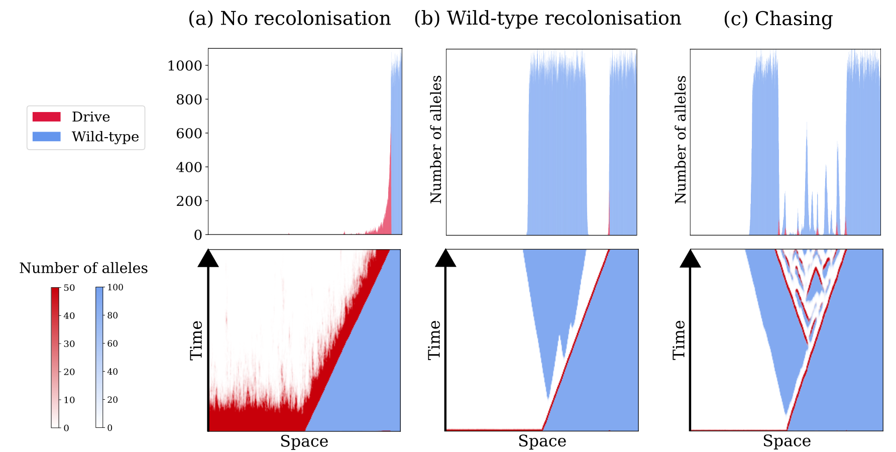
Figure 1: Illustrations of the different outcomes of drive propagation, presented as snapshots (top row, at a fixed time $t$) and kymographs (bottom row, from time $0$ to $t$), showing the different types of outcomes (columns). The drive fitness cost varies from low on the right column to high on the left column. Number of drive alleles (in red) and wild-type alleles (in blue) are represented on the y-axis in the top row, and in color intensities in the bottom row. The top row corresponds to a horizontal slice of the bottom row at the last time $t$. For a better visualisation, we adjusted the colormap of the bottom row to have saturation for 50 drive individuals and 100 wild-type individuals. The drive eradication wave might lead to different dynamics in space: (a) no recolonisation event at all, (b) wild-type recolonisation and persistence, (c) successive wild-type recolonisation and drive reinvasion (chasing).

Wild-type recolonisation events have been observed in compartmental models [13] and discrete individual-based models of eradication gene drive [11, 14, 15, 12, 16, 17, 18, 19, 20]. Previous studies have shown the influence of ecological factors on the chance of wild-type recolonisation after the spread of an eradication gene drive: high rates of dispersal reduce the chance of recolonisation [19, 12]; high levels of inbreeding increase the likelihood of recolonisation [12]; the presence of a competing species or predator facilitates extinction without recolonisation [17]. The release pattern of the drive seems to have little effect on recolonisation outcomes [12]. Drive fitness might also impact the risk of recolonisation: based on simulations, Champer et al. found that a higher fitness reduces the chance of recolonisation [12], while Paril and Phillips obtained contrasted results on X-shredder and W-shredder drives [19]. Building on these previous works, our study also investigates the impact of the drive’s fitness and the migration rate, but through an analytical approach supported by simulations. In addition, we explore the influence of the carrying capacity which, as far as we are aware, has not been done before. To simulate systems with very large numbers of individuals (up to $10^{12}$ on the whole domain), we implement our model in a population-based way, such that we follow the population size in each spatial site instead of the position of each living individual.

In this work, we focus on quantifying the probability that a wild-type recolonisation event does not occur within a realistic time window (Figure 1(a)). The rationale of this analysis is based on the following idea: if the last individual carrying a wild-type allele is surrounded by many drive individuals, then it is very unlikely that stochastic fluctuations can leave behind individuals carrying wild-type alleles capable of repopulating the empty place. On the contrary, if individuals carrying wild-type alleles are still present when the drive population is scarce, then it is conceivable that these individuals can recolonise with significant probability. Here, we will focus on the first facet of this rationale, using a deterministic approach to approximate the location of dense drive population. This approximation must however be completed with a stochastic approximation to determine the position of the last individual carrying at least one wild-type allele. We explain how to handle the deterministic parts in an analytical way, then we give some preliminary steps of how to deal with the stochastic part. The former is based on the theory of reaction-diffusion traveling waves, which was the main focus of [21], whereas the latter is based on a heuristical connection with extinction time in Galton-Watson branching processes. Interestingly, we find that, when parameters vary, most of the variation of the chance of recolonisation is due to the analytical contribution, for which we have explicit formulas.

To investigate the presence/absence of wild-type recolonisation events, we restrict our study case to a specific range of drive fitness values. Based on previous work [10, 21], we know that if the drive fitness is high enough, a drive monostable invasion occurs and the final drive proportion is 1. On the contrary if the drive fitness is low enough, a wild-type monostable invasion occurs and the final drive proportion is 0 (the drive wave retreats and the wild-type wave advances). For intermediate values of the drive fitness, we either observe bistable dynamics (the final drive proportion is either 0 or 1 depending on the initial condition) or coexistence final states (the final drive proportion is strictly between 0 and 1). Coexistence ensures genetic diversity at the back of the wave; we believe this would take us out of the rationale described above (the last individual carrying at least one wild-type allele is not surrounding by multiple drive individuals). Therefore we will not consider this case in this paper and restrict ourselves to the case of monostable drive invasion.

Our results suggest that the probability of wild-type recolonisation events increases with smaller fitness of drive individuals, smaller migration rate, and smaller local carrying capacity. To check the robustness of our analytical and numerical findings in one spatial dimension, we run stochastic simulations in two spatial dimensions varying both the fitness cost and the carrying capacity. The 2D results are consistent with the 1D case, except that wild-type recolonisation events happen faster in 2D than in 1D (as they can occur in a variety of directions). We also give analytical arguments to show that, in case of a wild-type recolonisation event, the probability of a following drive reinvasion event decreases with smaller values of the intrinsic growth rate of the population.

2 Models

2.1 Continuous deterministic model

We extend a model developed in previous articles [10, 21], assuming a partial conversion of rate $c\in(0,1)$ occurring in the germline. We assume that the individuals live in a one-dimensional space; they interact and reproduce locally, and they move in a diffusive manner. We therefore use a reaction diffusion framework. We denote by $n$ the total number of individuals in the population, by $n_{i}$ the number of individuals with genotype $i$ in the population, by $K$ the maximum carrying capacity of the environment, and by $\sigma^{2}$ the diffusion rate. Note that unlike our previous work [10, 21], we consider the number of individuals instead of the rescaled density. We follow three genotypes: wild-type homozygotes ($i=WW$), drive homozygotes ($i=DD$) and heterozygotes ($i=DW$). Wild-type homozygotes have fitness $f_{WW}=1$, drive homozygotes have fitness $f_{DD}=1-s$, where $s\in(0,1)$ is the fitness cost of the drive, and drive heterozygotes have fitness $f_{DW}=1-sh$, where $h\in(0,1)$ is the dominance parameter. The intrinsic growth rate is $r\in(0,+\infty)$, and we assume logistic growth, with density dependence affecting fecundity. We assume locally random mixing and we do not distinguish between sexes. With this, we obtain:

$$\left\{\small\begin{array}[]{ll}\partial_{t}n_{{}_{\mathrm{DD}}}-\sigma^{2}\partial_{xx}^{2}n_{{}_{\mathrm{DD}}}=(1-s)\left(r\ \left(1-\dfrac{n}{K}\right)+1\right)\ \dfrac{\frac{1}{4}\ (1+c)^{2}\ n_{{}_{\mathrm{DW}}}^{2}+(1+c)\ n_{{}_{\mathrm{DW}}}n_{{}_{\mathrm{DD}}}+n_{{}_{\mathrm{DD}}}^{2}}{n}-n_{{}_{\mathrm{DD}}},\\ \\ \partial_{t}n_{{}_{\mathrm{DW}}}-\sigma^{2}\partial_{xx}^{2}n_{{}_{\mathrm{DW}}}=(1-sh)\left(r\ \left(1-\dfrac{n}{K}\right)+1\right)\ \dfrac{(1+c)\ n_{{}_{\mathrm{WW}}}n_{{}_{\mathrm{DW}}}+2\ n_{{}_{\mathrm{WW}}}n_{{}_{\mathrm{DD}}}+\frac{1}{2}\ (1-c^{2})\ n_{{}_{\mathrm{DW}}}^{2}+(1-c)\ n_{{}_{\mathrm{DW}}}n_{{}_{\mathrm{DD}}}}{n}\\ \hskip 88.2037pt-n_{{}_{\mathrm{DW}}},\\ \\ \partial_{t}n_{{}_{\mathrm{WW}}}-\sigma^{2}\partial_{xx}^{2}n_{{}_{\mathrm{WW}}}=\left(r\ \left(1-\dfrac{n}{K}\right)+1\right)\ \dfrac{n_{{}_{\mathrm{WW}}}^{2}+(1-c)\ n_{{}_{\mathrm{WW}}}n_{{}_{\mathrm{DW}}}+\frac{1}{4}\ (1-c)^{2}\ n_{{}_{\mathrm{DW}}}^{2}}{n}-n_{{}_{\mathrm{WW}}}.\end{array}\right.$$ (1)

2.1.1 From genotypes to alleles

In [21], we established that model (1) can be reduced to two equations instead of three, focusing on allele numbers $(n_{{}_{\mathrm{D}}},n_{{}_{\mathrm{W}}})$ instead of genotype numbers $(n_{{}_{\mathrm{DD}}},n_{{}_{\mathrm{DW}}},n_{{}_{\mathrm{WW}}})$. The transformation is given by $n_{{}_{\mathrm{D}}}=n_{{}_{\mathrm{DD}}}+\alpha\ n_{{}_{\mathrm{DW}}}$ and $n_{{}_{\mathrm{W}}}=n_{{}_{\mathrm{WW}}}+(1-\alpha)\ n_{{}_{\mathrm{DW}}}$, with $\alpha=\frac{1+c}{2}$ when gene conversion occurs in the germline. With this transformation, system (1) is equivalent to the following one:

$$\left\{\begin{array}[]{ll}\partial_{t}n_{{}_{\mathrm{D}}}-\sigma^{2}\partial_{xx}^{2}n_{{}_{\mathrm{D}}}\ =\ n_{{}_{\mathrm{D}}}\ \Big{[}g_{{}_{\mathrm{D}}}(n_{{}_{\mathrm{D}}},n_{{}_{\mathrm{W}}})-1\Big{]},\\ \\ \partial_{t}n_{{}_{\mathrm{W}}}-\sigma^{2}\partial_{xx}^{2}n_{{}_{\mathrm{W}}}=\ n_{{}_{\mathrm{W}}}\ \Big{[}g_{{}_{\mathrm{W}}}(n_{{}_{\mathrm{D}}},n_{{}_{\mathrm{W}}})-1\Big{]},\end{array}\right.$$ (2)

where $g_{{}_{\mathrm{D}}}$ and $g_{{}_{\mathrm{W}}}$ are the per-capita growth rates associated with each allele, and are given by:

$$g_{{}_{\mathrm{D}}}(n_{{}_{\mathrm{D}}},n_{{}_{\mathrm{W}}})=\left(r\ \left(1-\dfrac{n}{K}\right)+1\right)\Big{[}(1-s)\dfrac{n_{{}_{\mathrm{D}}}}{n}+(1-sh)\ (1+c)\ \dfrac{n_{{}_{\mathrm{W}}}}{n}\Big{]},$$ (3a)

$$g_{{}_{\mathrm{W}}}(n_{{}_{\mathrm{D}}},n_{{}_{\mathrm{W}}})=\left(r\ \left(1-\dfrac{n}{K}\right)+1\right)\Big{[}\ \dfrac{n_{{}_{\mathrm{W}}}}{n}+(1-sh)\ (1-c)\ \dfrac{n_{{}_{\mathrm{D}}}}{n}\Big{]}.$$ (3b)

In the following, the term “number of drive alleles” (resp. “number of wild-type alleles”) refers to the quantities $n_{D}$ (resp. $n_{W}$), and represents an haploid count.

2.1.2 Drive invasion and traveling waves

As it is classical in spatial ecology [22], we investigate the spatial invasion of the drive allele by means of traveling waves. We seek stationary solutions in a reference frame moving at speed $v_{\text{co}}$ (“co” stands for continuous model),

$$\left\{\begin{array}[]{ll}n_{{}_{\mathrm{D}}}(t,x)=N_{{}_{\mathrm{D}}}(x-v_{\text{co}}t)=N_{{}_{\mathrm{D}}}(z)\quad\quad(\forall t>0)\ (\forall x\in\mathbb{R}),\\ n_{{}_{\mathrm{W}}}(t,x)=N_{{}_{\mathrm{W}}}(x-v_{\text{co}}t)=N_{{}_{\mathrm{W}}}(z)\quad\ \ (\forall t>0)\ (\forall x\in\mathbb{R}),\\ \end{array}\right.$$ (4)

Plugging this particular shape of a solution in (2), we deduce the following pair of equations for the traveling wave profiles ($N_{{}_{\mathrm{D}}}$, $N_{{}_{\mathrm{W}}}$):

$$\left\{\begin{array}[]{ll}-v_{\text{co}}N_{{}_{\mathrm{D}}}^{\prime}-\sigma^{2}N_{{}_{\mathrm{D}}}^{\prime\prime}&=\ N_{{}_{\mathrm{D}}}\ \left[\left(r\ \left(1-\dfrac{N}{K}\right)+1\right)\Big{[}(1-s)\dfrac{N_{{}_{\mathrm{D}}}}{N}+(1-sh)\ (1+c)\ \dfrac{N_{{}_{\mathrm{W}}}}{N}\Big{]}-1\right],\\ \\ -v_{\text{co}}N_{{}_{\mathrm{W}}}^{\prime}-\sigma^{2}N_{{}_{\mathrm{W}}}^{\prime\prime}&=\ N_{{}_{\mathrm{W}}}\ \left[\left(r\ \left(1-\dfrac{N}{K}\right)+1\right)\Big{[}\ \dfrac{N_{{}_{\mathrm{W}}}}{N}+(1-sh)\ (1-c)\ \dfrac{N_{{}_{\mathrm{D}}}}{N}\Big{]}-1\right].\end{array}\right.$$ (5)

We impose the following conditions:

$$\left\{\begin{array}[]{ll}v_{\text{co}}>0,\\ N_{{}_{\mathrm{D}}}(-\infty)=0\,,\quad N_{{}_{\mathrm{D}}}(+\infty)=0,\\ N_{{}_{\mathrm{W}}}(-\infty)=0\,,\quad N_{{}_{\mathrm{W}}}(+\infty)=1.\\ \end{array}\right.$$ (6)

These conditions mean that we consider a drive eradication wave propagating from the left-hand side to the right-hand side of our figures. A schematic illustration of the wave is drawn in Figure 4(a). In this mathematical framework, the limiting values $N_{{}_{\mathrm{D,W}}}(-\infty)=0$ listed in system (6) correspond to the eradication of the population after the drive wave has passed. The condition to attain this outcome reads $r<\frac{s}{1-s}$ [10, 21].

Traveling wave solutions contain important information for the biological interpretation of the results. The speed $v_{\text{co}}$ is the rate of propagation of the drive population. Under assumptions (6), the profile $N_{{}_{\mathrm{D}}}(z)$ has exponential decay both when $z$ goes to $+\infty$ and $-\infty$ (Figure 4(a)). The profile $N_{{}_{\mathrm{W}}}(z)$ has exponential decay when $z$ goes to $-\infty$. This can be expressed as follows:

At the front of the wave: $$N_{{}_{\mathrm{D}}}(z)\approx\exp\left(\lambda_{D,\ \text{co}}^{\text{front}}z\right),$$ (7a)

At the back of the wave: $$N_{{}_{\mathrm{D}}}(z)\approx\exp\left(\lambda_{D,\ \text{co}}^{\text{back}}z\right),$$ (7b)

At the back of the wave: $$N_{{}_{\mathrm{W}}}(z)\approx\exp\left(\lambda_{W,\ \text{co}}^{\text{back}}z\right).$$ (7c)

The rates of decay denoted by $\lambda$ play a key role in our analysis. It would be possible to derive several qualitative conclusions to some extent of generality, but we opt for simplicity, and we limit our analysis to the case of pulled traveling waves (see [21] for the notion of pulled versus pushed waves in the context of population eradication by a gene drive), because the speed $v_{\text{co}}$ is explicitly known in that case:

$$v_{\text{co}}=v_{\text{co}}^{\text{lin}}=2\sqrt{(1-sh)(1+c)-1}$$ (8)

(see Appendix B.1 for details).

We therefore assume that all the waves that we consider are pulled. As shown in [21], when gene conversion occurs in the germline, the drive wave is always pulled for $h<0.5$. In this study, we consider $h=0.4$ for the numerical illustrations. We obtain formulas for the exponential rates of profiles $n_{{}_{\mathrm{D}}}$ and $n_{{}_{\mathrm{W}}}$ at the front and at the back of the wave, namely:

$$\lambda_{D,\ \text{co}}^{\text{front}}= \frac{1}{\sigma}\left(-\sqrt{(1-sh)(1+c)-1}\right),$$ (9a)

$$\lambda_{D,\ \text{co}}^{\text{back}}= \frac{1}{\sigma}\left(-\sqrt{(1-sh)(1+c)-1}+\sqrt{(1-sh)(1+c)-(r+1)(1-s)}\right),$$ (9b)

$$\lambda_{W,\ \text{co}}^{\text{back}}= \frac{1}{\sigma}\left(-\sqrt{(1-sh)(1+c)-1}+\sqrt{(1-sh)(1+c)-(r+1)(1-sh)(1-c)}\right),$$ (9c)

(see Appendix B.1 for details).

2.2 Discrete stochastic model

To observe wild-type recolonisation events, we need to consider a stochastic discrete model, based on the allele dynamics described by system (2). We denote the number of drive and wild-type alleles at spatial site $x$ and time $t$ as:

$$n_{{}_{\mathrm{D}}}(t,x)=n_{{}_{\mathrm{D}}}^{t,x},\quad n_{{}_{\mathrm{W}}}(t,x)=n_{{}_{\mathrm{W}}}^{t,x}\quad\text{and}\quad n(t,x)=n^{t,x}\quad\quad\forall\ t\in\{0,dt,2dt,...\},\ \forall x\in\{0,dx,2dx,...\}.$$ (10)

In our stochastic simulations, each individual reproduces, dies and disperses independently of the reproduction, death, and dispersal of others. We alternate between two types of events: 1) allele production/disappearance in each spatial site and 2) allele migration in the neighbouring spatial sites. During one time unit, a drive allele duplicates on average $g_{{}_{\mathrm{D}}}(n_{{}_{\mathrm{D}}}^{t,x},n_{{}_{\mathrm{W}}}^{t,x})$ times, as defined in equation (3a), and a wild-type allele duplicates on average $g_{{}_{\mathrm{W}}}(n_{{}_{\mathrm{D}}}^{t,x},n_{{}_{\mathrm{W}}}^{t,x})$, as defined in equation (3b). One allele (drive or wild-type) disappears at rate $1$ within one time unit, corresponding to the death of an individual carrying it. To model the number of new alleles and removed alleles, we use Poisson distributions with these respective means. A Poisson distribution corresponds to the number of events observed during a time interval of given length, when the waiting time between two consecutive events is given by an exponential distribution. For one type of event, under an exponential distribution, the expected future waiting time is independent of waiting time already passed.

Second, we consider migration: at each time step, an allele migrates with probability $m$ outside its original site. It goes to one neighbouring spatial site, either on the right or on the left, with equal probabilities. To model this event, we use two Bernoulli distributions: one with probability $m$ to determine if the individual migrates, the second with probability $\frac{1}{2}$ in case of success, to determine the welcoming site (right or left).

Remark 1 (Migration rate vs. diffusion coefficient)

Both the migration rate (denoted $m$, discrete models) and the diffusion coefficient (denoted $\sigma^{2}$, continuous models) describe the ability of individuals to move in space. Their relationship is given by

$$\sigma^{2}=\dfrac{m(\Delta x)^{2}}{2\Delta t}.$$ (11)

We implement this model in a population-based way: we follow the number of alleles in each spatial site instead of following the position of each living individual (which would then be an individual-based model). In each site, we draw independent events of production/disappearance of alleles relative to the number of alleles in this site, and the same goes for migration events.

These dynamics are summarised in Figure 2 and the detailed code is provided in Appendix A. The main advantage of this approach is that it allows to simulate systems with very large number of alleles.

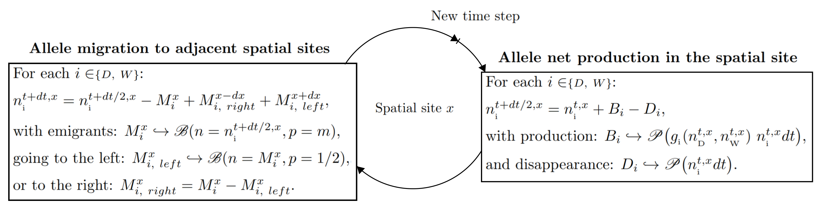
Figure 2: Consecutive steps in the stochastic discrete model.

The discrete model also exhibits finite speed propagation, but the rate of propagation differs from its continuous version (8) for two reasons: firstly, the stepping-stone discretisation, and secondly, the stochastic effects due to finite population size. These two corrections of the speed are very well documented [23, 24]. However, for the sake of simplicity, we prefer to conduct our analysis based on the formulas of the continuous model, as in Section 2.1. In the following sections, we briefly present each correction, and we compare the outcomes of the theory and the numerical simulations, in order to support our continuous approximation.

2.2.1 Correction of the speed due to the stepping stone discretisation

We consider a deterministic version of the discrete model, that is, the one obtained by considering the expectation in each site, which can be deduced in the limit of large carrying capacity $K\to+\infty$. When the wave is pulled, the speed $v_{\text{di}}$ is given by the following minimization problem (for details, see Section B.2):

$$v_{\text{di}}=v_{\text{di}}^{\text{lin}}=\underset{\lambda<0}{\min}\left(\mathscr{V}(\lambda)\right)=\underset{\lambda<0}{\min}\left(\dfrac{\log\left(\left[\left((1-sh)(1+c)-1\right)\ d\!t+1\right]\ \left[1-m+m\ \cosh(\lambda\ \ d\!x)\right]\right)}{-\lambda\ d\!t}\right),$$ (12)

which coincides with (8) in the limit $d\!t,d\!x\to 0$. The rates of (discrete) exponential decay can be deduced from (12), similarly as in (7) (see Appendix B.2 for detail). In particular, the rate of decay at the front, $\lambda_{D,\ \text{di}}^{\text{front}}$ is the $\lambda$ giving rise to the minimal value.

2.2.2 Correction of the speed due to the finite size of the population

The wave is pulled, meaning that its speed is determined by the few drive individuals at the front of the wave. The model being stochastic, small densities exhibit relatively stochastic fluctuations in their dynamics, so that the speed of propagation in stochastic simulations is smaller than (12). This discrepancy has been predicted analytically in [23, 24] (see also [25, 26] for the mathematical proof) to be:

$$v_{\text{di (cor)}}\approx v_{\text{di}}-\dfrac{\mathscr{V}^{\prime\prime}(\lambda_{D,\ \text{di}}^{\text{front}})\ \pi^{2}\ (\lambda_{D,\ \text{di}}^{\text{front}})^{2}}{2\ \left(\log\left(\frac{1}{K}\right)\right)^{2}},$$ (13)

where $v_{\text{di (cor)}}$ is the corrected discrete speed, and the function $\mathscr{V}$ is given in equation (12). This analytical prediction was obtained heuristically by a cut-off argument which takes into account the fact that the distribution of individuals vanishes beyond some finite range, in contrast with the continuous model where the density is positive everywhere.

In Table 1, we compare the following quantities, respectively for $s=0.3$ and $s=0.7$ (see Table 2 for the set of all parameters): i) the continuous speed $v_{\text{co}}$ given by (8); ii) the discrete speed $v_{\text{di}}$ given by (12); iii) the discrete speed corrected due to stochastic effects $v_{\text{di (cor)}}$ given by (13); and iv) the numerical speed $v_{\text{num}}$ as measured in stochastic numerical simulations. The best approximation of the speed computed numerically is indeed the corrected discrete speed, given by (13).

$s$ value	Speed
	$v_{\text{co}}$	$v_{\text{di}}$	$v_{\text{di (cor)}}$	$v_{\text{num}}$
$0.3$	$1.64$	$1.63$	$1.62$	$1.61$
$0.7$	$1.21$	$1.21$	$1.20$	$1.19$

Table 1: Comparison of the speed values for $s=0.3$ or $0.7$ and $K=10^{8}$; see Table 2 for the other parameter values. The continuous speed $v_{\text{co}}$ is given by (8), the discrete speed $v_{\text{di}}$ is given by (12), the correction of the discrete speed $v_{\text{di (cor)}}$ is given by (13) and the numerical speed $v_{\text{num}}$ is computed numerically.

2.3 Initial conditions and parameters for numerical simulations

Initial conditions for our numerical simulations are illustrated in Figure 3. The left half of the domain is full of drive alleles ($n_{{}_{\mathrm{D}}}=K$), and the right half is full of wild-type alleles ($n_{{}_{\mathrm{W}}}=K$). Reference to right or left positions are made in the context of this initial state.

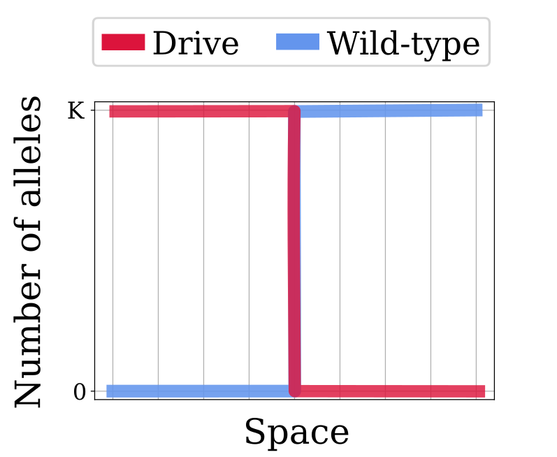
Figure 3: Initial conditions for numerical simulations in one spatial dimension.

Numerical simulations are performed with the same set of parameters (unless specified otherwise), summarised in Table 2. The code is available on GitHub (https://github.com/LenaKlay/gd_project_1/tree/main/stochastic). We ran our simulations in Python 3.6, with the Spyder environment.

Parameter	Range value	Value	Description
$r$	$(0,+\infty)$	$0.1$	Intrinsic growth rate
$c$	$[0,1]$	$0.9$	Conversion rate
$s$	$(0,1)$	$0.3$ or $0.7$	Fitness cost of drive homozygotes
$h$	$[0,1]$	$0.4$	Drive dominance
$m$	$[0,1]$	$0.2$	Migration rate
$K$	$(0,+\infty)$	from $10^{3}$ to $10^{8}$	Local carrying capacity
$dx$	$(0,1]$	$1$	Spatial step between two sites
$dt$	$(0,1]$	$0.1$	Temporal step
$T$	$(0,+\infty)$	$1000$	Simulation maximum time

Table 2: Model parameters and numerical values used in the simulations.

3 Results

3.1 Drive eradication waves in the continuous model

The parameters detailed in Section 2.3 have been chosen to verify two conditions in the deterministic model: i) the final equilibrium is an empty environment (eradication) ii) the drive invades for all initial conditions (monostable drive invasion). Such conditions establish a suitable framework for the observation of wild-type recolonisation events in the stochastic model (suitable but not sufficient). Figure 4(a) represents the typical outcome expected in the continuous model under these assumptions, with the two profiles $N_{D}$ (red) and $N_{W}$ (blue) and a speed of propagation $v$, as described by the set of equations (5)–(6). The relative intensities of exponential decay at the back of the wave are key to our analysis, see Figure 4(b).

The eradication condition is given by:

$$r<\frac{s}{1-s},$$ (14)

which is equivalent to $\lambda_{D,\ \text{co}}^{\text{back}}>0$ (9b). Hence, this demographic eradication condition is equivalent to having an exponential decay at the back of the wave, as expected.

The monostable drive invasion condition is given by:

$$(1-sh)(1+c)>1,$$ (15)

or equivalently denoted as $s<s_{2,g}$ in [21]. This condition ensures a strictly positive drive allele production at the front of the wave, as the production of drive alleles relies on heterozygotes (with a fitness of $(1-sh)$, a drive allele production rate of $(1+c)$ and a mortality rate of $1$). Indeed, wild-type alleles are so numerous at the front of the wave that at least one parent in each couple is wild-type homozygote (WW), and offspring carrying drive alleles are necessarily heterozygotes.

Remark 2 (Exclusion of the particular case of coexistence)

The monostable drive invasion condition does not exclude the existence of a final coexistence state, however, this case is rather easy to appreciate, which is why we address it separately in this remark. By definition, the coexistence case results in a final drive proportion strictly between $0$ and $1$ at the back of the wave in the continuous model [21]. The question raised in this article — "Is the last individual carrying a drive allele at the back of the wave surrounded by a sufficiently large number of drive alleles?" — would then receive a negative answer and we expect that such coexistence state would very likely lead to recolonisation events in stochastic simulations, due to a relatively large number of wild-type alleles in small population areas. Therefore, we add a third condition to exclude coexistence cases:

$$(1-sh)(1-c)<(1-s).$$ (16)

We insist on the fact that coexistence is only a relative equilibrium among frequencies, because this can occur while the whole population goes extinct (under condition (14)). We then observe a transition in the analytical computations and find $\lambda_{W,\ \text{co}}^{\text{back}}=\lambda_{D,\ \text{co}}^{\text{back}}$, meaning that the drive and wild-type alleles decay with the same exponential rate at the back of the wave, and that they both reach non-zero equilibrium frequencies at $-\infty$ in space. On the contrary, condition (16) denoted as $s<s_{1}$ in [21], is equivalent to $\lambda_{W,\ \text{co}}^{\text{back}}>\lambda_{D,\ \text{co}}^{\text{back}}$ ensuring that the drive curve is less steep than the wild-type curve as in Figure 4(b). Under condition (16), the final drive proportion reaches $1$ (and the final wild-type proportion reaches $0$) [21].

3.2 Stochastic recolonisation of the wild-type at the back of the wave

The continuous representation fails at very low number of alleles per site. This can be seen in Figures 4(c–f), showing the outcomes of stochastic simulations, and where the drive and the wild-type allelic distributions are plotted in log scale. Only the back of the wave is shown on these panels to focus on the occurrence of recolonisation events. Multiple time points are superimposed in these figures, and the curves are translated to have a constant number of wild-type alleles at the spatial origin on the right hand side (either 100 or 1000 alleles depending on the figures). The black lines are the exponential approximations for each, as described with detail in Appendix B.2 (they are the analogues of expressions (9) for the stepping stone discrete approximation). For a large drive fitness cost ($s=0.7$) and a relatively small carrying capacity ($K=10^{5}$), we observe one wild-type recolonisation event within this window of time (Figure 44(f)). Note that in this example, the slopes of the wild-type and drive curves are similar, and carrying capacity is relatively low.

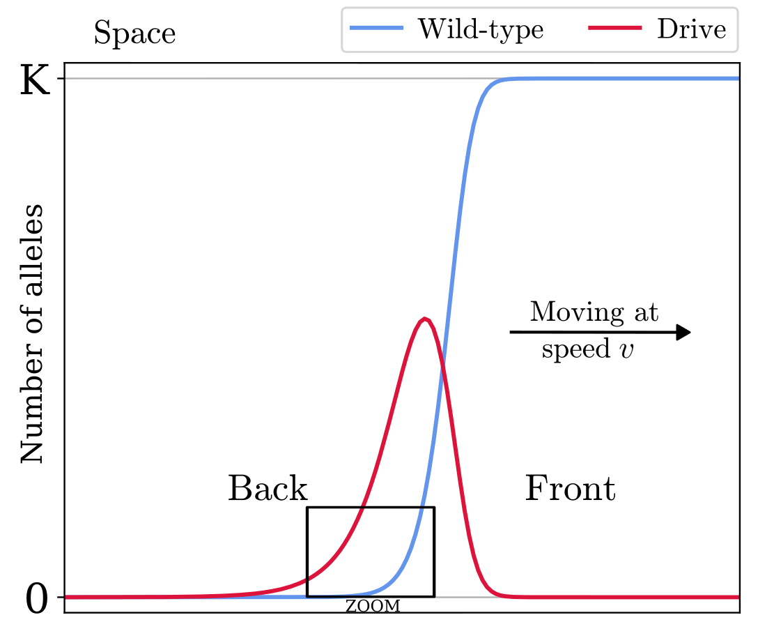
(a) Propagating wave in the continuous model

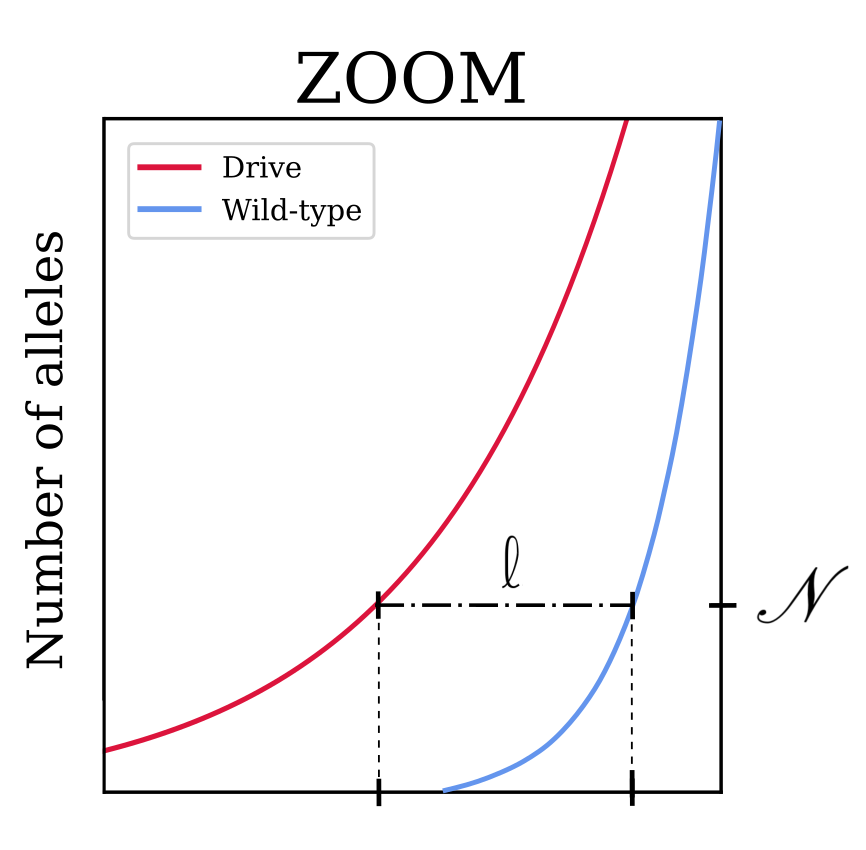
(b) Zoom at the back of the wave: both densities decay exponentially fast to zero in case of eradication

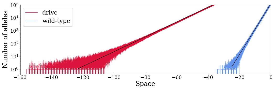
(c) $K=10^{8}$, $s=0.3$

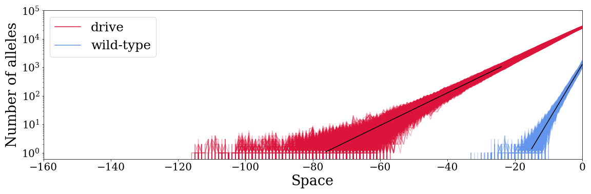
(d) $K=10^{5}$, $s=0.3$

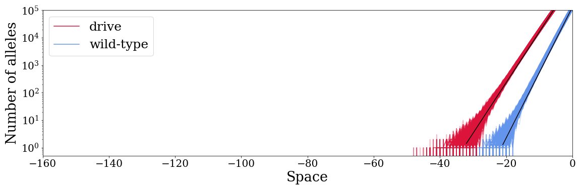
(e) $K=10^{8}$, $s=0.7$

(f) $K=10^{5}$, $s=0.7$ – Wild-type recolonisation

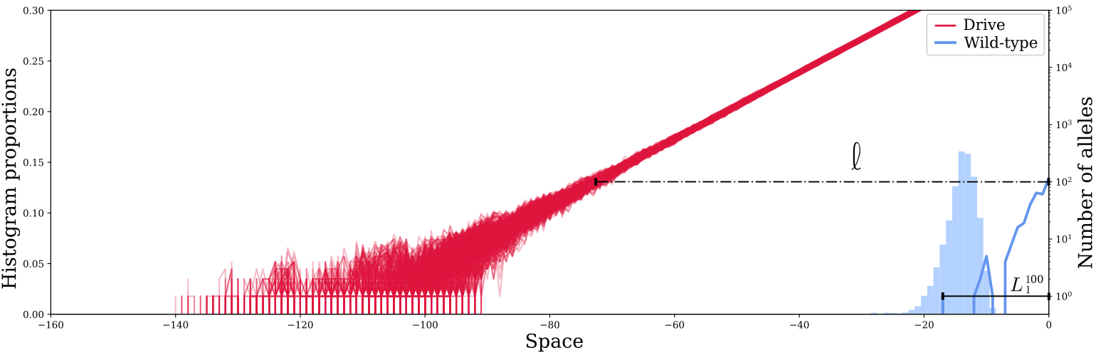
(g) $K=10^{8}$, $s=0.3$

Figure 4: Number of drive alleles (in red) and number of wild-type alleles (in blue) at the back of the wave, for the continuous model in linear scale (panels (a, b)) and the stochastic model in log scale (panels (c, d, e, f, g)). The points of abscissa $z=0$ is arbitrary placed at the last spatial site with more than $1000$ wild-type alleles in panels (c, d, e, f) and with more than $100$ wild-type alleles in panel (g). We superimpose multiple realisations corresponding to 2000 different timepoints in the simulation, to observe the stochastic variations. The exponential approximations from Appendix B.2 are shown for each wave in black. We observe a wild-type recolonisation event for $s=0.7$ and $K=10^{5}$. In panel (g), for $s=0.3$ and $K=10^{8}$, we add in the figure a histogram showing the spatial distribution of the last wild-type allele in lighter blue, highlighting the high stochasticity of this position.

3.3 A theoretical framework to characterize the absence of recolonisation

We posit that wild-type recolonisation or chasing can very likely be prevented if the last individual carrying a wild-type allele is surrounded by a sufficiently large number of drive individuals. This reference number, denoted by $\mathscr{N}$, should be large enough to avoid stochastic effects, but much smaller than the carrying capacity $K$. We choose $\mathscr{N}=100$ in this paper.

To get a clearer view, we superimpose in Figure 4(g) the distribution of drive alleles at several times ($n_{{}_{\mathrm{D}}}$ in red), the distribution of wild-type alleles at a single time ($n_{{}_{\mathrm{W}}}$ in blue) and the histogram of the position of the last wild-type allele (light blue). We see that a clear separation exists between the distribution of the last wild-type allele and the area with few drive alleles (below 100) when $s=0.3$ preventing the wild-type recolonisation with high probability.

3.4 Spatial separation

To determine when wild-type recolonisation or chasing is very unlikely, and evaluate the contributions of each parameter, we aim to separate the space between a deterministic zone and a stochastic zone at the back of the wave, depending on the number of alleles per site.

We denote by $\ell$ the distance between the last position with more than $\mathscr{N}$ drive alleles and the last position with more than $\mathscr{N}$ wild-type alleles, illustrated in Figure 4(g). We make the strong hypothesis that this distance can be well approximated by a deterministic model. This entails choosing $\mathscr{N}$ sufficiently large. Moreover, to ease the analytical calculations, we are going to use the spatially continuous model rather than the discrete one for the values of $\lambda$ characterizing the curves.

The second quantity of interest is $L_{1}^{\mathscr{N}}$, the distance between the position of the last individual carrying a wild-type allele and the last position with more than $\mathscr{N}$ wild-type alleles, also illustrated in Figure 4(g). In contrast to $\ell$, this distance is genuinely stochastic.

Figure 5 represents the distribution of the furthest spatial positions associated with at least $\mathscr{N}=100$ drive alleles (in red) and $\mathscr{N}=100$ wild-type alleles (in blue), and the furthest spatial position associated with a single wild-type allele in the site, that is, the position of the last individual carrying a wild-type allele. We clearly see that the two former distributions are concentrated around a deterministic value, whereas the latter is more spread out.

We can recast our mathematical problem as $L_{1}^{\mathscr{N}}<\ell$ with high probability, meaning that the last wild-type individuals is very likely surrounded by more than $\mathscr{N}$ alleles, which is clearly the case in Figure 5(a) for small value of the drive fitness cost $s$ ($s=0.3$). In contrast, when $s$ is larger ($s=0.7$), the last wild-type allele is possibly surrounded by relatively few drive alleles when $s=0.7$, because the distribution of the position of the last wild-type allele (light blue) falls beyond the distribution of the last site with more than $\mathscr{N}=100$ alleles (Figure 5(b)). Note that deterministic distance $\ell$ (between the red and blue distributions) accounts for most of the variation when $s$ decreases, while stochastic distance $L_{1}^{\mathscr{N}}$ (between the light blue and blue distributions) remains similar.

Here, the value of $\mathscr{N}$ is quite arbitrary, but it has little influence on the mathematical argument. Our conclusions will be mainly qualitative, as we are lacking analytical predictions, in particular about the stochastic part $L_{1}^{\mathscr{N}}$.

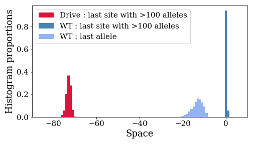
(a) $K=10^{8}$, $s=0.3$

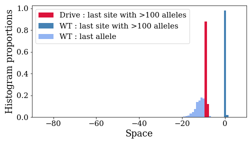
(b) $K=10^{8}$, $s=0.7$

Figure 5: Relative positions of the last spatial site with more than 100 drive alleles at the back of the wave (in red), the last spatial site with more than 100 wild-type alleles at the back of the wave (in blue) and the last wild-type allele at the back of the wave (in light blue). We collected these positions at 2000 different time points during the simulation to plot these histograms. We arbitrary set the last spatial site with more than $100$ wild-type alleles at the points of abscissa $z=0$. The statistical distribution of the last wild-type individuals is highly stochastic in contrast with the two other involving more than $100$ alleles. We also observe that this distribution is not symmetric, indicating rare events of last individuals carrying a wild-type allele being far away at the back of the wave. Note that deterministic distance $\ell$ (between the red and blue distributions) accounts for most of the variation, while stochastic distance $L_{1}^{\mathscr{N}}$ (between the light blue and blue distributions) remains similar.

3.5 The deterministic distance $\ell$

In the deterministic continuous approximation at the back of the wave, the quantity $\ell$ corresponds to the distance between the two points of abscissa $z_{D}$ and $z_{W}$ such that

$$\rho_{D}^{\text{back}}K\exp{(\lambda_{D,\ \text{co}}^{\text{back}}z_{D})}=\rho_{W}^{\text{back}}K\exp{(\lambda_{D,\ \text{co}}^{\text{back}}z_{W})}=\mathscr{N}.$$ (17)

The factor $\rho_{D}^{\text{back}}\in(0,1)$ , resp. $\rho_{W}^{\text{back}}\in(0,1)$, is characterized by the shape of the continuous traveling wave profile $N_{D}$, resp. $N_{W}$. We arbitrary set $\mathcal{N}$ so that the continuous profile is accurately approximated by an exponential ramp for $z<0$, see Figure 4(b). This leads to the following approximation for $\ell$ with $z_{D}<z_{W}<0$:

$$\text{$\ell$}=z_{W}-z_{D}=\dfrac{1}{\lambda_{W,\ \text{co}}^{\text{back}}}\log\left(\frac{\mathscr{N}}{\rho_{W}^{\text{back}}K}\right)-\dfrac{1}{\lambda_{D,\ \text{co}}^{\text{back}}}\log\left(\frac{\mathscr{N}}{\rho_{D}^{\text{back}}K}\right),$$ (18)

with the decay exponents $\lambda_{W,\ \text{co}}^{\text{back}}$ (9b) and $\lambda_{D,\ \text{co}}^{\text{back}}$ (9b). The next three sections are devoted to the analytical investigation of the influence of the carrying capacity $K$, the diffusion coefficient $\sigma^{2}$ and the drive fitness cost $s$ on distance $\ell$. Figure 6 illustrates numerically distance $\ell$ with respect to the carrying capacity and the drive fitness cost.

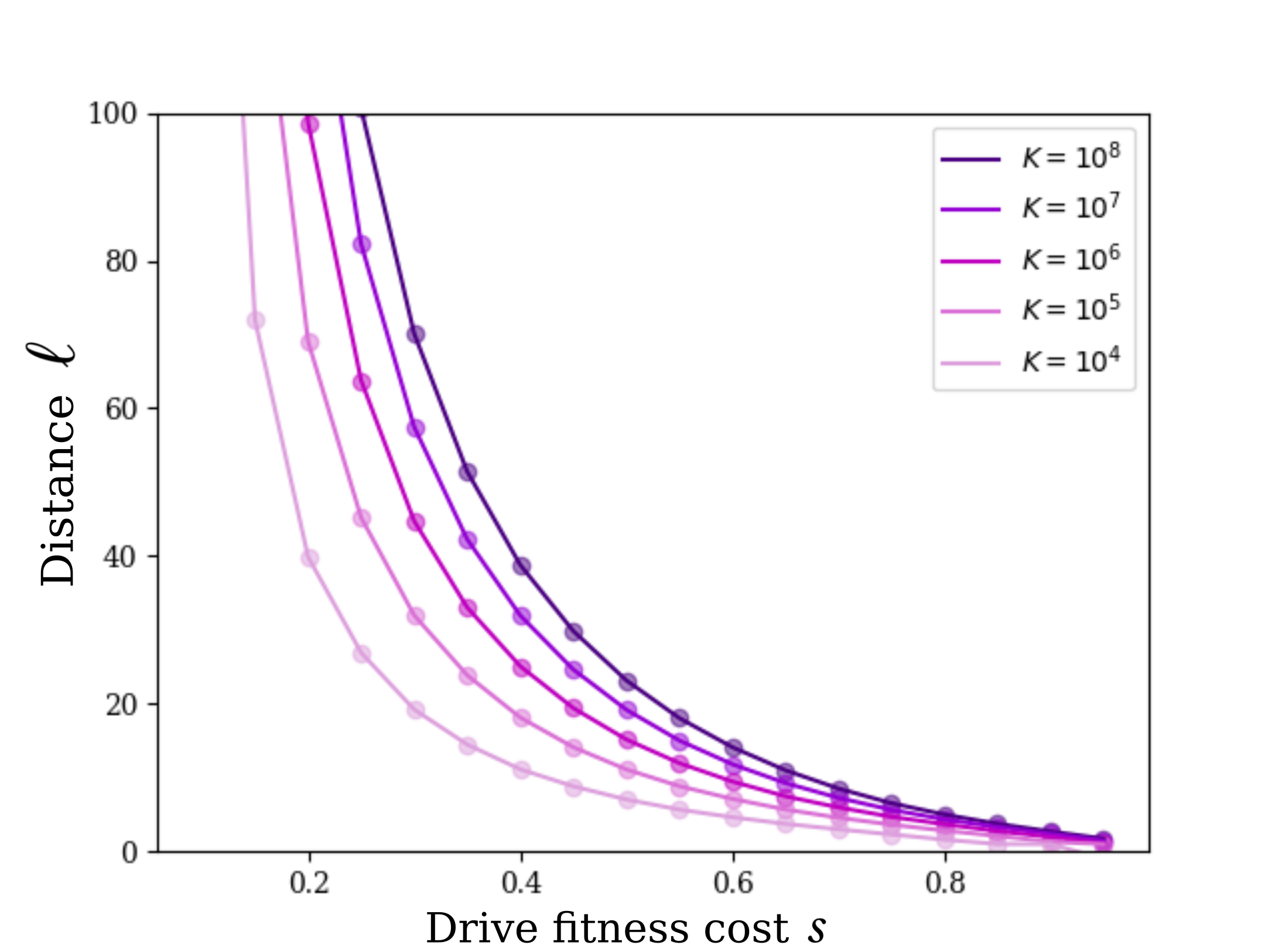
Figure 6: Distance $\ell$ for different values of the carrying capacity $K$ and the drive fitness cost $s$, computed through deterministic simulations as in [21]. The distance $\ell$ increases with $K$ and decreases with $s$.

3.5.1 The deterministic distance $\ell$ is increasing with the carrying capacity $K$

The carrying capacity $K$ influences the height of the spatial profile without changing the slope values at the back of the wave ($\lambda_{D,\ \text{co}}^{\text{back}}$ is independent from $K$). From equation (18), we know that distance $\ell$ increases with respect to the carrying capacity $K$. More precisely, if the carrying capacity is multiplied by a factor $10$, then $\ell$ increases by $\log(10)\left(\dfrac{1}{\lambda_{D,\ \text{co}}^{\text{back}}}-\dfrac{1}{\lambda_{W,\ \text{co}}^{\text{back}}}\right)$. This quantity is strictly positive under condition (16). Note that in case of a coexistence state (excluded from the study), $\ell$ would not increase with $K$ as $\lambda_{W,\ \text{co}}^{\text{back}}=\lambda_{D,\ \text{co}}^{\text{back}}$.

3.5.2 The deterministic distance $\ell$ is increasing with the diffusion coefficient $\sigma^{2}$

The influence of the diffusion rate $\sigma^{2}$ can be appreciated by noting that $\lambda_{D,\ \text{co}}^{\text{back}}$ (9b) and $\lambda_{W,\ \text{co}}^{\text{back}}$ (9b) are inversely proportional to $\sigma$. Therefore, $\ell$ is proportional to $\sigma$ (equation (18)) and increases with the migration rate $m$ (Remark 1).

3.5.3 The deterministic distance $\ell$ is decreasing with the drive fitness cost $s$

In this section, we determine the sign of the derivative of $\ell=z_{W}-z_{D}$ regarding to the drive fitness cost $s$. This part is the most technical one. Indeed, it is not complicated to see that both $z_{W}$ and $z_{D}$ are decreasing with respect to the fitness cost $s$, but establishing the monotonicity of the difference is more involved. We begin with an approximation of $\ell$ to ease the computations:

$$\ell=\left(\dfrac{1}{\lambda_{W,\ \text{co}}^{\text{back}}}-\dfrac{1}{\lambda_{D,\ \text{co}}^{\text{back}}}\right)\log\left(\frac{\mathscr{N}}{K}\right)+\dfrac{1}{\lambda_{W,\ \text{co}}^{\text{back}}}\log\left(\frac{1}{\rho_{W}}\right)-\dfrac{1}{\lambda_{D,\ \text{co}}^{\text{back}}}\log\left(\frac{1}{\rho_{D}}\right)\sim\left(\dfrac{1}{\lambda_{W,\ \text{co}}^{\text{back}}}-\dfrac{1}{\lambda_{D,\ \text{co}}^{\text{back}}}\right)\log\left(\frac{\mathscr{N}}{K}\right)$$ (19)

as $\rho_{W}<1\ll K/\mathscr{N}$, and $\rho_{D}<1\ll K/\mathscr{N}$ in logarithmic scale. Below we are going to establish analytically that

$$\dfrac{d}{ds}\left(\dfrac{1}{\lambda_{W,\ \text{co}}^{\text{back}}}-\dfrac{1}{\lambda_{D,\ \text{co}}^{\text{back}}}\right)>0,$$ (20)

leading to the conclusion that $\ell$ is decreasing with $s$ in the approximation (19) because $\log\left(\frac{\mathscr{N}}{K}\right)<0$. Instead of comparing the two explicit solutions $\lambda_{D,\ \text{co}}^{\text{back}}$ and $\lambda_{W,\ \text{co}}^{\text{back}}$, we start from the characteristic equations satisfied by each component. The following equations can be deduced from (5), and lead to the formulas (9), see Section B.1.2 for details.

$$0=\sigma^{2}(\lambda_{D,\ \text{co}}^{\text{back}})^{2}+v_{\text{co}}^{\text{lin}}\lambda_{D,\ \text{co}}^{\text{back}}+\Big{[}(r+1)(1-s)-1\Big{]},$$ (21)

$$0=\sigma^{2}(\lambda_{W,\ \text{co}}^{\text{back}})^{2}+v_{\text{co}}^{\text{lin}}\lambda_{W,\ \text{co}}^{\text{back}}+\Big{[}(r+1)(1-sh)(1-c)-1\Big{]}.$$ (22)

For the sake of simplicity, we introduce a notation for the zeroth order coefficients:

$$q_{D}(s)=(r+1)(1-s)-1\quad\text{and}\quad q_{W}(s)=(r+1)(1-sh)(1-c)-1,$$ (23)

and the (common) velocity wave for which we recall the formula:

$$v(s)=v_{\text{co}}^{\text{lin}}=2\sigma\sqrt{(1-sh)(1+c)-1}.$$ (24)

We differentiate each equation (21) and (22) with respect to $s$, and we find:

$$0=\sigma^{2}2\lambda_{D,\ \text{co}}^{\text{back}}(s)\frac{d\lambda_{D,\ co}^{\text{back}}}{ds}(s)+v(s)\frac{d\lambda_{D,\ co}^{\text{back}}}{ds}(s)+\frac{dv}{ds}(s)\lambda_{D,\ \text{co}}^{\text{back}}(s)+\frac{dq_{D}}{ds}(s),$$ (25)

$$0=\sigma^{2}2\lambda_{W,\ \text{co}}^{\text{back}}(s)\frac{d\lambda_{W,\ co}^{\text{back}}}{ds}(s)+v(s)\frac{d\lambda_{W,\ co}^{\text{back}}}{ds}(s)+\frac{dv}{ds}(s)\lambda_{W,\ \text{co}}^{\text{back}}(s)+\frac{dq_{W}}{ds}(s),$$ (26)

from which we deduce:

$$\frac{d}{ds}\left(\dfrac{1}{\lambda_{D,\ \text{co}}^{\text{back}}}\right)(s)=\dfrac{v^{\prime}(s)\lambda_{D,\ \text{co}}^{\text{back}}(s)+q_{D}^{\prime}(s)}{\lambda_{D,\ \text{co}}^{\text{back}}(s)^{2}(\sigma^{2}2\lambda_{D,\ \text{co}}^{\text{back}}(s)+v(s))}=F\left(q_{D}^{\prime},\lambda_{D,\ \text{co}}^{\text{back}}\right),$$ (27)

$$\frac{d}{ds}\left(\dfrac{1}{\lambda_{W,\ \text{co}}^{\text{back}}}\right)(s)=\dfrac{v^{\prime}(s)\lambda_{W,\ \text{co}}^{\text{back}}(s)+q_{W}^{\prime}(s)}{\lambda_{W,\ \text{co}}^{\text{back}}(s)^{2}(\sigma^{2}2\lambda_{W,\ \text{co}}^{\text{back}}(s)+v(s))}=F\left(q_{W}^{\prime},\lambda_{W,\ \text{co}}^{\text{back}}\right).$$ (28)

We are going to use the monotonicity properties of $F$ combined with some useful properties about $q_{D},q_{W}$ and $\lambda_{D,\ \text{co}}^{\text{back}},\lambda_{W,\ \text{co}}^{\text{back}}$ in order to establish the chain of inequalities leading to the result

$$F\left(q_{D}^{\prime},\lambda_{D,\ \text{co}}^{\text{back}}\right)<F\left(q_{D}^{\prime},\lambda_{W,\ \text{co}}^{\text{back}}\right)<F\left(q_{W}^{\prime},\lambda_{W,\ \text{co}}^{\text{back}}\right).$$

Firstly, the function $F$ is increasing with respect to the variable $\lambda$:

$$\begin{split}\frac{\partial F}{\partial\lambda}(q,\lambda)&=\dfrac{v^{\prime}\lambda^{2}(\sigma^{2}2\lambda+v)-(v^{\prime}\lambda+q^{\prime})(\sigma^{2}6\lambda^{2}+2v\lambda)}{\lambda^{4}(\sigma^{2}2\lambda+v)^{2}}\\ &=\dfrac{-4\sigma^{2}v^{\prime}\lambda^{3}-vv^{\prime}\lambda^{2}-6\sigma^{2}q^{\prime}\lambda^{2}-2vq^{\prime}\lambda}{\lambda^{4}(\sigma^{2}2\lambda+v)^{2}}>0.\end{split}$$ (29)

In fact, each term in the above numerator is positive: $-v^{\prime}(s)>0$ (24), and $-q^{\prime}(s)>0$, both for $q_{D}^{\prime}$ and $q_{W}^{\prime}$ (23). When this partial monotonicity is combined with the aforementioned fact that $\lambda_{W,\ \text{co}}^{\text{back}}>\lambda_{D,\ \text{co}}^{\text{back}}$ (condition (16)), we get that

$$F\left(q_{D}^{\prime},\lambda_{D,\ \text{co}}^{\text{back}}\right)<F\left(q_{D}^{\prime},\lambda_{W,\ \text{co}}^{\text{back}}\right)$$ (30)

Secondly, the function $F$ is clearly increasing with respect to the variable $q^{\prime}$. Moreover, we have $q_{D}^{\prime}(s)=-(r+1)<-(1-c)h(r+1)=q_{W}^{\prime}(s)<0$, because $(1-c)h<1$. Therefore, we can deduce that

$$F\left(q_{D}^{\prime},\lambda_{W,\ \text{co}}^{\text{back}}\right)<F\left(q_{W}^{\prime},\lambda_{D,\ \text{co}}^{\text{back}}\right).$$ (31)

Bringing inequalities (30) and (31) together, we obtain:

$$\frac{d}{ds}\left(\dfrac{1}{\lambda_{D,\ \text{co}}^{\text{back}}}\right)=F\left(q_{D}^{\prime},\lambda_{D,\ \text{co}}^{\text{back}}\right)<F\left(q_{W}^{\prime},\lambda_{W,\ \text{co}}^{\text{back}}\right)=\frac{d}{ds}\left(\dfrac{1}{\lambda_{W,\ \text{co}}^{\text{back}}}\right),$$ (32)

from which we deduce (20) and the fact that $\ell$ is decreasing with respect to $s$.

Remark 3 (Intrinsic fitness vs. fitness cost)

In the literature, the intrinsic fitness $\mathdutchcal{f}_{\mathrm{D}}$ is sometimes considered instead of the fitness cost $s$. The drive intrinsic fitness is the overall ability of drive alleles to increase in frequency when the drive proportion is close to zero. Its value is closely linked with $s$, and given by first line of system (2):

$$\mathdutchcal{f}_{\mathrm{D}}=(1-sh)(1+c)-1\quad\iff\quad s=\dfrac{c-\mathdutchcal{f}_{\mathrm{D}}}{h(1+c)}.$$ (33)

The fitness $\mathdutchcal{f}_{\mathrm{D}}$ and the fitness cost $s$ are in negative relationship, so that any conclusion on the influence of $s$ can be immediately transferred to $\mathdutchcal{f}_{\mathrm{D}}$.

3.6 The stochastic distance $L_{1}^{\mathscr{N}}$

We now consider the position of the last individual carrying a wild-type allele, for which stochastic effects are predominant (Figure 5). The aim of this section is to draw a parallel with spatial Galton-Watson processes in a fixed frame, for which there exists a mathematical theory – see for instance [27].

Galton-Watson processes describe a single isolated population in time, based on the assumption that individuals give birth and die independently of each other, and follow the same distribution for each of these events. It appears that Galton-Watson processes with migration are very sensitive to spatial parameters: as we work on a limited spatial domain, we focus on extinction time instead of distance to the last wild-type allele, less affected by this restriction.

We need to verify two assumptions before heuristically reducing our stochastic problem to a spatial Galton-Watson process: i) first, the stochastic distance $L_{1}^{\mathscr{N}}$ ($L^{100}_{1}$ in the following) can be transformed into an extinction time problem and ii) second, the dynamics of the wild-type alleles at the back of the wave can be approximated by a stochastic process of an ideal population consisting of wild-type alleles only in a isolated space.

In the following, the positions of the last wild-type allele and the extinction times are all computed conditionally to the absence of wild-type recolonisation in the global simulation: as we try to characterise the conditions preventing wild-type recolonisation in a realisable time window, we assume that recolonisation has not happened yet.

3.6.1 Converting distances to extinction times

We denote by $L_{0}^{100}$ the distance between the empty site right on the left of the last wild-type allele, and the last position with more than $100$ wild-type alleles at the back of the wave. We have:

$$L_{0}^{100}=L_{1}^{100}+dx,$$ (34)

with $dx$ the size of a spatial step. We also define $T^{100}_{0}$ as the time that the last spatial site with more than $100$ wild-type alleles (at the back of the wave) takes to go extinct. As the wave is moving at a constant speed $v_{\text{num}}$, we ask whether the distance $L_{0}^{100}$ follows the same distribution as the time $T^{100}_{0}$ multiplied by the speed of the wave ($v_{\text{num}}$). Figure 7 shows the two distributions for two values of the drive fitness cost $s=0.3$ and $s=0.7$. In both cases, they appear very close from each other, which validates our first assumption.

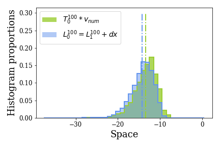
(a) $s=0.3$

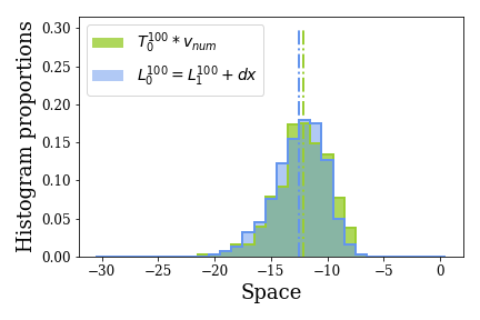
(b) $s=0.7$

Figure 7: Superimposition of the statistical distributions of distance $L_{0}^{100}$ (in light blue) and extinction time $T^{100}_{0}$ multiplied by the speed of the wave $v_{\text{num}}$ (in light green). These distributions are calculated for $K=10^{8}$, over 500 different time points. The two distributions are very close for $s=0.3$, and for $s=0.7$. The distribution of $L_{1}^{100}$, the relative position of the last wild-type individual is asymmetric, like already observed in Figure 5; this asymmetry is preserved in the distribution of extinction time $T^{100}_{0}$ times speed $v_{\text{num}}$.

3.6.2 From a global dynamics to an isolated population

We now ask whether the time $T^{100}_{0}$ (time that the last spatial site with more than 100 wild-type individuals at the back of the wave takes to go extinct) can be approximated by the extinction time $T^{100}_{0\ \text{gw}}$ of a single isolated population modelled with an auxiliary stochastic stepping stone process. We consider a spatial Galton-Watson process in a fixed domain, where the population is distributed with an exponential spatial profile at initial time. At the back of the wave and in the absence of wild-type recolonisation, we assume that:

$$\dfrac{n_{{}_{\mathrm{D}}}^{t,x}}{n^{t,x}}\sim 1\ ,\ \dfrac{n_{{}_{\mathrm{W}}}^{t,x}}{n^{t,x}}\ll 1\ \ \text{and}\ \ n^{t,x}\ll 1.$$ (35)

We know from (3b) that a wild-type allele at the back of the wave produces on average $g_{{}_{\mathrm{W}}}(n_{{}_{\mathrm{D}}}^{t,x},n_{{}_{\mathrm{W}}}^{t,x})$ alleles (in offspring) during one time unit, with

$$g_{{}_{\mathrm{W}}}(n_{{}_{\mathrm{D}}}^{t,x},n_{{}_{\mathrm{W}}}^{t,x})=\left(r\ (1-\frac{n^{t,x}}{K})+1\right)\left[\ \dfrac{n_{{}_{\mathrm{W}}}^{t,x}}{n^{t,x}}+(1-sh)\ (1-c)\ \dfrac{n_{{}_{\mathrm{D}}}^{t,x}}{n^{t,x}}\right]\approx(r+1)(1-sh)(1-c),$$ (36)

and disappears on average at rate $1$. Thanks to this approximation, the dynamics do not depend on $n_{{}_{\mathrm{D}}}$ any more, and we can simulate a single isolated wild-type population. As before, at each time step, a wild-type allele migrates to the adjacent site on the right with probability $\frac{m}{2}$ and to the left with probability $\frac{m}{2}$.

To be consistent in the comparison between $T^{100}_{0}$ (global dynamics) and $T^{100}_{0\ \text{gw}}$ (single population approximation), we initiate the simulation with the profile $\exp(z\ \lambda_{W,\ \text{di}}^{\text{back}})$ approximating the exponential decay of wild-type allele numbers at the back of the wave (Section 2.2.1). We also observe that migration from dense areas to less dense areas in the exponential profile plays a major role and significantly increases the extinction time $T^{100}_{0\ \text{gw}}$ (Appendix C). Thus, we had to consider a large exponential initial condition with a maximum number of individuals per site being $10^{6}$, to fully capture the wild-type dynamics at the end of the wave.

To obtain the statistical distribution of $T^{100}_{0\ \text{gw}}$, we run the simulation $500$ times. In Figure 8, we superimpose this distribution (multiply by the speed of the wave $v_{\text{num}}$ to obtain a distance) with the distribution of $T^{100}_{0}$ (also multiplied by $v_{\text{num}}$). The histograms are very close for $s=0.3$ and $s=0.7$: our second assumption is verified. This result paves the way for further analysis; if one was able to characterise analytically extinction time $T^{100}_{0\ \text{gw}}$ of this spatial Galton Watson process, we would also have an analytical approximation of distance $L^{100}_{0}$ and consequently, an analytical condition ensuring the absence of wild-type recolonisation event with high probability in a realisable time window.

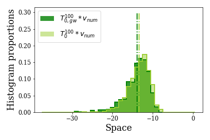
(a) $s=0.3$

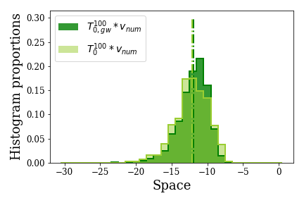
(b) $s=0.7$

Figure 8: Superimposition of the statistical distributions of extinction times $T^{100}_{0}$ (in light green) and $T^{100}_{0\ \text{gw}}$ (in dark green), multiplied by the speed of the wave $v_{\text{num}}$ to obtain distances. The extinction time $T^{100}_{0}$ is collected over 500 different time points in the global dynamics, while $T^{100}_{0\ \text{gw}}$ is obtained running the spatial Galton-Watson process detailed in the main text 500 times. The distribution of $T^{100}_{0\ \text{gw}}$ (single population approximation) fits very well the distribution of $T^{100}_{0}$ (global dynamics) and the asymmetry is again preserved.

3.7 Numerical conclusions

In Figure 4(g), the probability to observe one wild-type recolonisation event in a realisable time window is extremely low when $s=0.3$: the furthest away the last individual carrying a wild-type allele might be is a spatial site with more than $10^{4}$ drive alleles. However, when $s=0.7$, this very last position corresponds to a number of drive alleles below $100$ (Figure 5 (b), and consequently, a non-negligible chance of wild-type recolonisation.

In Figure 9, we numerically approximate the probability to observe wild-type recolonisation within $1000$ units of time, for different values of $s$ the drive fitness cost and $K$ the local carrying capacity. Each point of the graph is determined by the proportion of replicates where we observe wild-type recolonisation, over $100$ replicates. This probability increases with $s$ and decreases with $K$. Noticeably for a given local carrying capacity $K$, the transition between very low ($<10\%$) and very high ($>90\%$) chances of wild-type recolonisation within $1000$ units of time when the fitness cost $s$ varies, is relatively restricted: these two extreme conditions can be reached at two different $s$ values within a range of $0.2$.

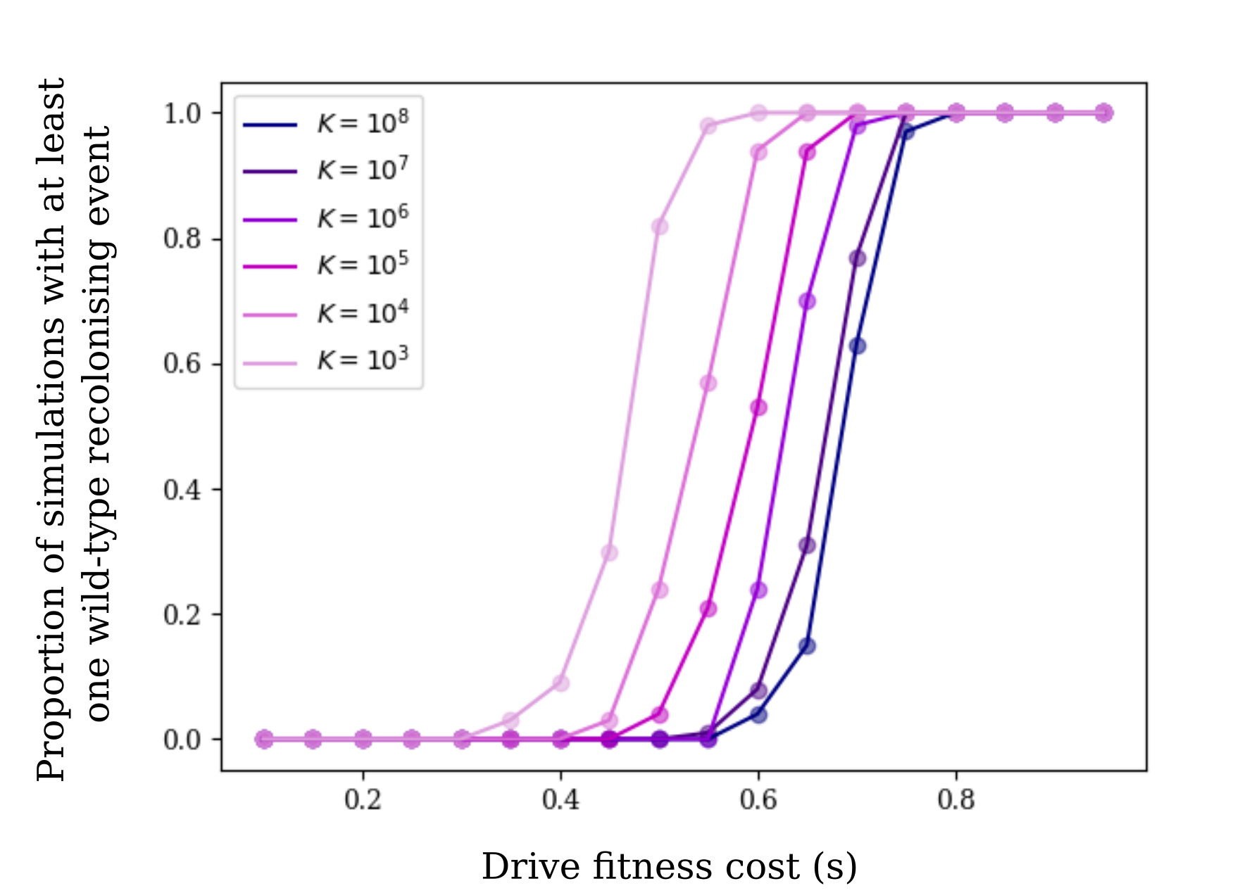
Figure 9: Proportion of simulations encountering at least one wild-type recolonisation event within $1000$ units of time, as a function of $s$, the fitness disadvantage for drive, and $K$, the carrying capacity on one spatial step. For each point, we ran $100$ simulations. When $K=10^{8}$, the probability to observe wild-type recolonisation over $1000$ units of time is close to $0$ for $s=0.3$, and approximately $0.63$ when $s=0.7$.

3.8 Comparison with the two-dimensional case

We extend the 1D stochastic model to a 2D version, using the same probabilistic framework. Traveling waves now move in multiple directions at the same time, instead of one.

In Figure 10, we compare the numerical outcomes for medium versus large carrying capacity ($K=10^{5}$ and $K=10^{8}$), and small versus high fitness cost ($s=0.3$ and $s=0.7$). Similarly to the one-dimensional case, we observe in 2D that the probability of wild-type recolonisation events increases with higher drive fitness cost and smaller carrying capacity. Note that $\lambda_{D,\ \text{co}}^{\text{back}}$ and $\lambda_{W,\ \text{co}}^{\text{back}}$ formulas stay unchanged in 2D, meaning that all analytical results from Section 3.5 still hold.

The main discrepancy between 1D and 2D simulations relies on the fact that rare stochastic events tend to happen on average faster in 2D than in 1D, as they can occur in a variety of directions each time. For small drive fitness cost, the probability of wild-type recolonisation event is so low that 1D and 2D simulations result in the same outcome of complete extinction (Figure 10(a,b)). However for higher fitness cost, wild-type recolonisation events occur faster in 2D than in 1D (Figure 10(c,d)). Similarly, we only observe drive reinvasion event(s) in the 2D simulations within this time window (Figure 10(c,d)). Additional simulations in line with these observations are shown in Appendix D, with a smaller carrying capacity $K=10^{3}$.

(a) $K=10^{8},s=0.3$

(b) $K=10^{5},s=0.3$

(c) $K=10^{8},s=0.7$

(d) $K=10^{5},s=0.7$

Figure 10: Comparison between the 1D and the 2D stochastic models, using the same numerical framework, with drive fitness cost $s=0.3$ or $s=0.7$ and carrying capacity $K=10^{3}$ ou $K=10^{5}$. Wild-type alleles are shown in blue and drive alleles in red. In 1D, the y-axis represents the number of alleles, while in 2D, the number of alleles is shown in shades of colour: the darker the colour, the more alleles of the corresponding type on the spatial site. For small drive fitness cost $s=0.3$, both 1D and 2D simulations show similar outcomes, i.e. the full eradication of the population. For high drive fitness cost $s=0.7$, the system is more sensitive to wild-type recolonisation events. The 2D domain amplifies this discrepancy: it facilitates the emergence of rare events as they can occur in a variety of directions each time. As expected, a larger carrying capacity reduces the stochasticity and consequently the probability of wild-type recolonisation event, both in 1D and 2D.

3.9 From wild-type recolonisation events to chasing dynamics

To ensure eradication in the vast majority of cases, we focus in this paper on a condition under which wild-type recolonisation is highly unlikely. However, eradication also seems plausible after a wild-type recolonisation event followed by several drive reinvasion events, as observed in Figure 10(d) 2D. In this section, we briefly explore the drive reinvasion dynamics, and whether they could eventually result in the eradication of the population.

We first introduce the three-step cycle underlying chasing dynamics (Figure 11). The cycle is composed of a wild-type stochastic recolonisation event (A) occurring with probability $p_{A}\in(0,1)$, a drive stochastic reinvasion event (B) occurring with probability $p_{B}\in(0,1)$, and the eradication following the drive (re)invasion (C) occurring with probability $p_{C}=1$ under Condition (14). If $p_{A}\gg p_{B}$, we would expect a full wild-type recolonisation, whereas if $p_{B}\gg p_{A}$, we would expect the population to be fully eradicated. Infinite chasing dynamics might emerge when $p_{A}$ and $p_{B}$ get closer.

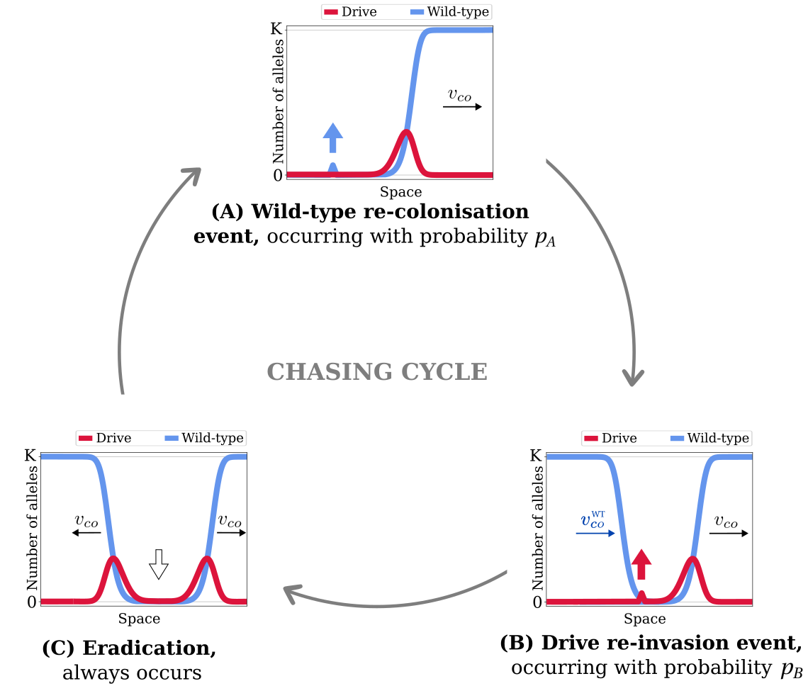
Figure 11: Illustration of the the three-step cycle underlying chasing dynamics. Wild-type recolonisation event (A) and drive reinvasion event (B) are stochastic events occurring with probabilities $p_{A},p_{B}\in(0,1)$, while the eradication following the drive (re)invasion (C) occurs with probability $p_{C}=1$ under Condition (14). If $p_{A}\gg p_{B}$, we would expect a full wild-type recolonisation, whereas if $p_{B}\gg p_{A}$, we would expect the population to be fully eradicated. Infinite chasing dynamics might emerge when $p_{A}$ and $p_{B}$ get closer.

To explore the probability of drive reinvasion $p_{B}$, we position ourselves in time when the wild-type recolonisation wave is already formed behind the drive eradication wave, as shown in panel (B) from Figure 11. The wild-type recolonisation wave travels at speed $v_{\text{co}}^{{}_{\mathrm{\text{WT}}}}$ (given by the second line of system (2) with $n_{{}_{\mathrm{D}}}=0$) while the drive eradication wave travels at speed $v_{\text{co}}$ (see Section 2.1.2):

$$v_{\text{co}}^{{}_{\mathrm{\text{WT}}}}=2\sqrt{r}\quad\quad\text{and}\quad\quad v_{\text{co}}=2\sqrt{(1-sh)(1+c)-1},$$ (37)

with $r$ the intrinsic growth rate. If $v_{\text{co}}^{{}_{\mathrm{\text{WT}}}}$ is small enough compared to $v_{\text{co}}$, drive reinvasion events are unlikely to occur as the two waves increasingly move apart (illustration in Figure 1(b)).

The eradication final state observed in Figure 10(d) 2D seems to result from a relatively higher probability of drive reinvasion compare to the probability of wild-type recolonisation ($p_{B}\gg p_{A}$). To confirm this intuition, we try to reverse the dynamics by artificially reducing the value of $r$: by slowing down the wild-type recolonisation wave ($v_{\text{co}}^{{}_{\mathrm{\text{WT}}}}$ decreases), we would reduce the probability of drive reinvasion. We choose $r=0.02$ instead of $r=1$, changing the value of $v_{\text{co}}^{{}_{\mathrm{\text{WT}}}}$ from approximately $0.632$ to $0.283$, and plot the comparison in Figure 12. The value of $v_{\text{co}}$ stays unchanged, approximately $1.213$ (with $s=0.7$, and $c$ and $h$ given in Table 2). As expected when $r=0.02$, the wild-type wave remains far behind the drive eradication wave, disabling drive reinvasion events and we witness a full wild-type recolonisation (Figure 12(a)). Several other cases have been investigated in Appendix E, all supporting this intuition.

(a) $r=0.02$

(b) $r=0.1$

Figure 12: Comparison of 2D numerical simulations for two different values of the intrinsic growth rate $r=0.02$ or $0.1$, with carrying capacity $K=10^{5}$ and drive fitness cost $s=0.7$. The case $r=0.1$ corresponds to Figure 10(d). On one hand, when $r=0.02$, the wild-type wave remains far behind the drive eradication wave, disabling drive reinvasion events; we witness a full wild-type recolonisation. On the other hand, when $r=0.1$, the wild-type recolonisation event is shortly followed by at least three drive reinvasion events, which lead to the complete eradication of the population.

4 Discussion

Given both the promise and risk of eradication drives, their dynamics are worthy of careful examination. In this work, we introduced a theoretical framework to characterise the conditions leading to successful extinction of a population targeted by an eradication gene drive. We sought to delimit the conditions for the absence of wild-type recolonisation in a pulled drive eradication wave in a realisable time window. More precisely, we considered that if the last individual carrying a wild-type allele is surrounded by a large number of drive individuals (set to $\mathscr{N}=100$ alleles in this work) then wild-type recolonisation is very unlikely. To attest if this is the case, we determined the distance between the last individual carrying a wild-type allele and the last spatial site with more than $100$ drive alleles, at the back of the wave. This value is not straightforward to find, so we proceeded in two steps.

First, we determined the distance $\ell$ between the drive and the wild-type wave at the level line corresponding to $100$ alleles. This distance is almost deterministic, as we chose $\mathscr{N}=100$ large enough for stochastic fluctuations to be negligible. We deduced this distance from a deterministic simulation and analytically proved that it increases with the carrying capacity $K$, increases with the migration rate $m$ and decreases with the drive fitness cost $s$. We also found that if the carrying capacity $K$ is multiplied by a factor $10$, the distance $\ell$ increases by $\left(\frac{1}{\lambda_{D,\ \text{di}}^{\text{back}}}-\frac{1}{\lambda_{W,\ \text{di}}^{\text{back}}}\right)\log(10)$, with $\lambda_{D,\ \text{di}}^{\text{back}}$, resp. $\lambda_{W,\ \text{di}}^{\text{back}}$, the exponent of the exponential profile at the back of the drive, resp. wild-type, wave. All these analytical results still hold in 2D.

Second, we determined the distance $L^{100}_{1}$ between the position of the last wild-type allele and the last position with more than $100$ wild-type alleles. This distance highly depends on the stochastic fluctuations of the last individual, and its distribution is difficult to characterise. To simplify the problem, we considered an isolated wild-type population, and we reduced heuristically the distance distribution to an extinction time distribution of a spatial Galton-Watson process, with the appropriate initialisation. Multiplying this time by the speed of the wave, we obtained a good approximation of the distance $L^{100}_{1}$. We leave open the quality of this approximation in mathematical terms, as well as the analysis of the distribution of the extinction time.

Combining the two distances $\ell$ and $L^{100}_{1}$ allowed us to determine precisely the conditions under which wild-type recolonisation is highly unlikely. Numerically, we observed that distance $L^{100}_{1}$ shows little variation, indicating that most of the variation is due to the distance $\ell$, which varies inversely with the probability of wild-type recolonisation. The larger the carrying capacity is, the fewer recolonisation events we observe numerically. And the fitter the drive, the smaller the chance of wild-type recolonisation, in agreement with the results obtained in [12]. Noticeably in our study, the transition between very low ($<10\%$) and very high ($>90\%$) chances of wild-type recolonisation when the drive fitness cost varies is relatively restricted: for $s$ the drive fitness cost varying between $0$ (no drive fitness cost) and $1$ (no possible survival for drive individuals), this happens within a range of $0.2$. Focusing on the drive intrinsic fitness, i.e. the overall ability of drive to increase in frequency when the drive proportion is close to zero, we agree on the observations made by [19]: the fitter the drive, the sharper the drive wave at the front (9a), and the faster the speed (8) as initially showed in [28]. In contrast at the back of the wave, the fitter the drive, the wider the drive wave, reducing the risk of wild-type recolonisation (see Section 3.5.3). We also demonstrated that if we consider the same migration rate for all genotypes, high migration rates would reduce the chance of wild-type recolonisation. This result is in agreement with the numerical observations made in [19, 12].

The outcomes of our 2D simulations are consistent with our 1D conclusions: the probability of wild-type recolonisation events increases with higher drive fitness cost and smaller carrying capacity. Nevertheless, we observe that stochastic events (both wild-type recolonisation and drive reinvasion events) emerge in average more frequently in 2D than in 1D, leading to faster dynamics. This is due to the fact that stochastic events can occur in a variety of directions each time in 2D, instead of only one in 1D.

Finally, we explored the drive reinvasion dynamics after one (or a few) hypothetical wild-type recolonisation event(s). We demonstrated that the probability of drive reinvasion depends on the speed of both the wild-type recolonizing wave and the drive eradication wave, and decreases with smaller values of the intrinsic growth rate $r$. If the probability of drive reinvasion is way higher than the probability of wild-type recolonisation, we expect the population to go extinct.

The models that we used in this study are generalist: they could be applied to different species and gene drive constructs. They provide general conclusions but also come with necessary simplifications. For instance, we assumed a uniform landscape with random movement, which is extremely rare in the wild. Realistic migration patterns over both small and large scales would need to be taken into account to obtain better predictions. In mosquito populations, gene drive propagation can be accelerated by long distance migrations: mosquitoes can benefit from fast air currents (transporting them for hundreds of kilometres in a few hours) [29, 30, 31] or human-based modes of travel such as cars [32] or planes [33]. This could make it easier for wild-type individuals to permeate the drive wave, and initiate the recolonisation of empty areas.

A variety of other ecological parameters must also be taken into account before any field release. A previous study showed that the presence of a competing species or predator in the ecosystem could make eradication substantially easier than anticipated and prevent wild-type recolonisation [17]. The life cycle of the species, the survival characteristics, the mating system, the ecological differences between males and females, the seasonal population fluctuations are all biological characteristics that might also influence outcomes.

The type of gene drive constructs might also bias our prediction depending on how the fitness disadvantage impacts the individual (in our model, it impacts the birth rate) and the possible emerging resistances that might alter the gene conversion ability of the drive (we consider a constant conversion rate $c$) [34, 35, 36, 1].

Because of its generic nature, our model cannot be used directly for risk assessment, but informs, qualitatively, on the potential failure of an eradication drive.

Appendix

Appendix A Implementation of the stochastic model

⬇

1### Initialization

2

3# Number of individuals in each spatial site

4nD = np.zeros(nb_sites).astype(int); nD[:nb_sites//2] = K*dx # Drive individuals

5nW = np.zeros(nb_sites).astype(int); nW[nb_sites//2:] = K*dx # Wild-type individuals

6# Fecundity

7fD = np.zeros(nb_sites) # Drive fecundity

8fW = np.zeros(nb_sites) # Wild-type fecundity

9

10

11### Evolution in time

12

13for t in np.arange(0, T, dt):

14

15 ### Stop the simulation if the wave goes outside the window

16

17 if np.where(nD==max(nD))[0][0] > len(nD)-10 :

18 print("t =",t)

19 break

20

21 ### Birth and Death

22

23 # Index for empty and non empty sites

24 extinct_index = np.where(nD+nW==0)[0]

25 survive_index = np.delete(np.arange(nb_sites), extinct_index)

26 # Fecundity for non empty sites

27 sv_pop = nD[survive_index] + nW[survive_index]

28 sv_nD = nD[survive_index]; sv_nW = nW[survive_index]

29 fD[survive_index] = ( 1+r*(1-sv_pop/(K*dx)) ) * ( (1-s)*sv_nD + (1-s*h)*(1+c)*sv_nW ) /sv_pop

30 fW[survive_index] = ( 1+r*(1-sv_pop/(K*dx)) ) * ( (1-c)*(1-s*h)*sv_nD + sv_nW ) /sv_pop

31 # For empty sites, the fecundity is 0.

32 fD[extinct_index] = 0

33 fW[extinct_index] = 0

34 # Add births and substract deaths (mortality = 1)

35 nD = nD + np.random.poisson(fD*nD*dt) - np.random.poisson(nD*dt)

36 nW = nW + np.random.poisson(fW*nW*dt) - np.random.poisson(nW*dt)

37 # Transform negative number of individuals into 0

38 nD[np.where(nD<0)[0]]=0

39 nW[np.where(nW<0)[0]]=0

40

41

42 ### Migration

43

44 # Number of migrants in each site

45 nD_mig = np.random.binomial(nD,m)

46 nW_mig = np.random.binomial(nW,m)

47 # Half migrate to the right, half to the left

48 nD_mig_left = np.random.binomial(nD_mig,0.5); nD_mig_right = nD_mig - nD_mig_left

49 nW_mig_left = np.random.binomial(nW_mig,0.5); nW_mig_right = nW_mig - nW_mig_left

50 # Substract the migrants leaving

51 nD -= nD_mig

52 nW -= nW_mig

53 # ... except for those going outside the windows (they stay in the border site)

54 nD[0] += nD_mig_left[0]; nW[0] += nW_mig_left[0]

55 nD[-1] += nD_mig_right[-1]; nW[-1] += nW_mig_right[-1]

56 # Add the migrants in the neighboor sites

57 nD[1:] += nD_mig_right[:-1]; nW[1:] += nW_mig_right[:-1]

58 nD[:-1] += nD_mig_left[1:]; nW[:-1] += nW_mig_left[1:]

Appendix B Speed and exponential approximations of the wave

B.1 Continuous model

Since the wave is pulled, we deduce the speed $v_{\text{co}}$ and the exponential approximations at the back and at the front of the wave from system (5) as detailed in the following sections.

B.1.1 At the front of the wave

At the front of the wave, we assume that:

$$\dfrac{N_{{}_{\mathrm{D}}}}{N}\ll 1\ ,\ \dfrac{N_{{}_{\mathrm{W}}}}{N}\sim 1\ \ \text{and}\ \ N\sim 1.$$ (38)

Combined with system (5), we know the solution of equation (39) is an approximation of $N_{{}_{\mathrm{D}}}$ at the front of the wave:

$$0=\sigma^{2}N_{{}_{\mathrm{D}}}^{\prime\prime}+v_{\text{co}}N_{{}_{\mathrm{D}}}^{\prime}+N_{{}_{\mathrm{D}}}\ \Big{[}(1-sh)\ (1+c)-1\Big{]}.$$ (39)

Since the wave is pulled, the speed $v_{\text{co}}$ is given by the minimal speed $v_{\text{co}}^{\text{lin}}$ of the problem linearised at low drive allele numbers at the front of the wave. We approximate the decreasing drive section at the front of the wave by an exponential function of the form $N_{{}_{\mathrm{D}}}(z)\approx\rho_{D}^{front}\exp(\lambda_{D,\ \text{co}}^{\text{front}}z)$:

$$0=\sigma^{2}(\lambda_{D,\ \text{co}}^{\text{front}})^{2}+v_{\text{co}}\ \lambda_{D,\ \text{co}}^{\text{front}}+\Big{[}(1-sh)\ (1+c)-1\Big{]},$$ (40)

with the determinant $\Delta=(v_{\text{co}})^{2}-4\sigma^{2}\Big{[}(1-sh)\ (1+c)-1\Big{]}$. The minimal speed $v_{\text{co}}^{\text{lin}}$ is given by $\Delta=0$, thus:

$$v_{\text{co}}^{\text{lin}}=2\sigma\sqrt{(1-sh)(1+c)-1},$$ (41)

and the corresponding exponent is given by:

$$\lambda_{D,\ \text{co}}^{\text{front}}=-\dfrac{v_{\text{co}}^{\text{lin}}}{2\sigma^{2}}=-\dfrac{1}{\sigma}\sqrt{(1-sh)(1+c)-1}.$$ (42)

The quantity $(1-sh)(1+c)-1$ is always strictly positive for a pulled wave in case of drive invasion [21].

B.1.2 At the back of the wave

At the back of the wave, we assume that:

$$\dfrac{N_{{}_{\mathrm{D}}}}{N}\sim 1\ ,\ \dfrac{N_{{}_{\mathrm{W}}}}{N}\ll 1\ \ \text{and}\ \ N\ll 1.$$ (43)

By definition of a traveling wave, the speed at the front and at the back of the wave is equal.

Drive increasing section

Using (43) in system (5), we know the solution of the following equation (44) is an approximation of $N_{{}_{\mathrm{D}}}$ at the back of the wave:

$$0=\sigma^{2}N_{{}_{\mathrm{D}}}^{\prime\prime}+v_{\text{co}}^{\text{lin}}N_{{}_{\mathrm{D}}}^{\prime}+N_{{}_{\mathrm{D}}}\ \Big{[}(r+1)(1-s)-1\Big{]}.$$ (44)

We approximate the increasing drive section at the back of the wave by an exponential function of the form $N_{{}_{\mathrm{D}}}(z)\approx\rho_{D}^{\text{back}}\exp(\lambda_{D,\ \text{co}}^{\text{back}}z)$ and deduce from (44):

$$0=\sigma^{2}(\lambda_{D,\ \text{co}}^{\text{back}})^{2}+v_{\text{co}}^{\text{lin}}\lambda_{D,\ \text{co}}^{\text{back}}+\Big{[}(r+1)(1-s)-1\Big{]}r.$$ (45)

The solutions are given by:

$$\{\lambda_{D,\ \text{co}}^{\text{back}}\}_{+,-}= \dfrac{1}{2\sigma^{2}}\left(-v_{\text{co}}^{\text{lin}}\pm\sqrt{(v_{\text{co}}^{\text{lin}})^{2}-4\sigma^{2}\Big{[}(r+1)(1-s)-1\Big{]}}\ \right),$$ (46)

$$= \dfrac{1}{2\sigma^{2}}\left(-2\sigma\sqrt{(1-sh)(1+c)-1}\pm\sqrt{4\sigma^{2}\Big{[}(1-sh)(1+c)-1\Big{]}-4\sigma^{2}\Big{[}(r+1)(1-s)-1\Big{]}}\ \right),$$

$$= \frac{1}{\sigma}\left(-\sqrt{(1-sh)(1+c)-1}\pm\sqrt{(1-sh)(1+c)-1+1-(r+1)(1-s)}\right.$$

Since we study an eradication drive, we have $r<\dfrac{s}{1-s}\iff 1-(r+1)(1-s)>0$ [21]. Therefore, the two solutions of (46) are of opposite sign. At the back of the wave, the number of drive individuals tends to zero when $z\to-\infty$ therefore we only conserve the positive solution of (46).

$$\lambda_{D,\ \text{co}}^{\text{back}}=\frac{1}{\sigma}\left(-\sqrt{(1-sh)(1+c)-1}+\sqrt{(1-sh)(1+c)-(r+1)(1-s)}\right).$$ (47)

Wild-type increasing section

Using (43) in system (5), we know the solution of the following equation (48) is an approximation of $N_{{}_{\mathrm{W}}}$ at the back of the wave:

$$0=\sigma^{2}N_{{}_{\mathrm{W}}}^{\prime\prime}+vN_{{}_{\mathrm{W}}}^{\prime}+N_{{}_{\mathrm{W}}}\Big{[}(r+1)(1-sh)(1-c)-1\Big{]}.$$ (48)

We approximate the increasing wild-type section at the back of the wave by an exponential function of the form $N_{{}_{\mathrm{W}}}(z)\approx\rho_{W}^{\text{back}}\exp(\lambda_{W,\ \text{co}}^{\text{back}}z)$ and deduce from (48):

$$0=\sigma^{2}(\lambda_{W,\ \text{co}}^{\text{back}})^{2}+v_{\text{co}}^{\text{lin}}\lambda_{W,\ \text{co}}^{\text{back}}+\Big{[}(r+1)(1-sh)(1-c)-1\Big{]}.$$ (49)

The solutions are given by:

$$\dfrac{1}{2\sigma^{2}}\left(-v_{\text{co}}^{\text{lin}}\pm\sqrt{(v_{\text{co}}^{\text{lin}})^{2}-4\sigma^{2}\Big{[}(r+1)(1-sh)(1-c)-1\Big{]}}\ \right),$$ (50)

$$= \dfrac{1}{2\sigma^{2}}\left(-2\sigma\sqrt{(1-sh)(1+c)-1}\pm\sqrt{4\sigma^{2}\Big{[}(1-sh)(1+c)-1\Big{]}-4\sigma^{2}\Big{[}(r+1)(1-sh)(1-c)-1\Big{]}}\ \right),$$

$$= \frac{1}{\sigma}\left(-\sqrt{(1-sh)(1+c)-1}\pm\sqrt{(1-sh)(1+c)-1+1-(r+1)(1-sh)(1-c)}\right).$$

Since we study an eradication drive, we have $r<\dfrac{s}{1-s}\iff r+1<\dfrac{1}{1-s}$ [21] and therefore :

$$(r+1)(1-sh)(1-c)<\dfrac{1-sh}{1-s}(1-c)<1-c<1$$ (51)

The two solutions of (LABEL:eq:lWb) are of opposite sign. At the back of the wave, the number of wild-type individuals tends to zero when $z\to-\infty$: we only conserve the positive solution of (LABEL:eq:lWb).

$$\lambda_{W,\ \text{co}}^{\text{back}}=\frac{1}{\sigma}\left(-\sqrt{(1-sh)(1+c)-1}+\sqrt{(1-sh)(1+c)-(r+1)(1-sh)(1-c)}\right)$$ (52)

B.2 Discrete model

To determine the speed of the wave and the exponential approximations in the discrete stochastic model, we focus on the mean dynamics. For drive alleles, we have:

$$\left\{\small\begin{array}[]{ll}n_{{}_{\mathrm{D}}}^{t+\frac{dt}{2},x}&=\left((g_{{}_{\mathrm{D}}}(n_{{}_{\mathrm{D}}}^{t,x},n_{{}_{\mathrm{W}}}^{t,x})-1)\ dt+1\right)\ n_{{}_{\mathrm{D}}}^{t,x},\\ \\ n_{{}_{\mathrm{D}}}^{t+dt,x}&=(1-m)\ n_{{}_{\mathrm{D}}}^{t+\frac{dt}{2},x}+\dfrac{m}{2}\ (n_{{}_{\mathrm{D}}}^{t+\frac{dt}{2},x+dx}+n_{{}_{\mathrm{D}}}^{t+\frac{dt}{2},x-dx}),\end{array}\right.$$ (53)

and for wild-type alleles:

$$\left\{\small\begin{array}[]{ll}n_{{}_{\mathrm{W}}}^{t+\frac{dt}{2},x}&=\left((g_{{}_{\mathrm{W}}}(n_{{}_{\mathrm{D}}}^{t,x},n_{{}_{\mathrm{W}}}^{t,x})-1)dt+1\right)\ n_{{}_{\mathrm{W}}}^{t,x},\\ \\ n_{{}_{\mathrm{W}}}^{t+dt,x}&=(1-m)\ n_{{}_{\mathrm{W}}}^{t+\frac{dt}{2},x}+\dfrac{m}{2}\ (n_{{}_{\mathrm{W}}}^{t+\frac{dt}{2},x+dx}+n_{{}_{\mathrm{W}}}^{t+\frac{dt}{2},x-dx,}).\end{array}\right.$$ (54)

where the first lines correspond to the birth and death dynamics, and the second lines correspond to the migration. Combining the two lines in each system, we obtain:

$$\left\{\small\begin{array}[]{ll}n_{{}_{\mathrm{D}}}^{t+dt,x}&=\left((g_{{}_{\mathrm{D}}}(n_{{}_{\mathrm{D}}}^{t,x},n_{{}_{\mathrm{W}}}^{t,x})-1)\ dt+1\right)(1-m)\ n_{{}_{\mathrm{D}}}^{t,x}+\left((g_{{}_{\mathrm{D}}}(n_{{}_{\mathrm{D}}}^{t,x+dx},n_{{}_{\mathrm{W}}}^{t,x+dx})-1)\ dt+1\right)\dfrac{m}{2}\ n_{{}_{\mathrm{D}}}^{t,x+dx}\\ \\ &+\left((g_{{}_{\mathrm{D}}}(n_{{}_{\mathrm{D}}}^{t,x-dx},n_{{}_{\mathrm{W}}}^{t,x-dx})-1)\ dt+1\right)\dfrac{m}{2}\ n_{{}_{\mathrm{D}}}^{t,x-dx},\\ \\ n_{{}_{\mathrm{W}}}^{t+dt,x}&=\left((g_{{}_{\mathrm{W}}}(n_{{}_{\mathrm{D}}}^{t,x},n_{{}_{\mathrm{W}}}^{t,x})-1)dt+1\right)(1-m)\ n_{{}_{\mathrm{W}}}^{t,x}+\left((g_{{}_{\mathrm{W}}}(n_{{}_{\mathrm{D}}}^{t,x+dx},n_{{}_{\mathrm{W}}}^{t,x+dx})-1)dt+1\right)\dfrac{m}{2}\ n_{{}_{\mathrm{W}}}^{t,x+dx}\\ \\ &+\left((g_{{}_{\mathrm{W}}}(n_{{}_{\mathrm{D}}}^{t,x-dx},n_{{}_{\mathrm{W}}}^{t,x-dx})-1)dt+1\right)\dfrac{m}{2}\ n_{{}_{\mathrm{W}}}^{t,x-dx}.\end{array}\right.$$ (55)

with:

$$g_{{}_{\mathrm{D}}}(n_{{}_{\mathrm{D}}},n_{{}_{\mathrm{W}}})=\left(r\ (1-n)+1\right)\Big{[}(1-s)\dfrac{n_{{}_{\mathrm{D}}}}{n}+(1-sh)\ (1+c)\ \dfrac{n_{{}_{\mathrm{W}}}}{n}\Big{]},$$ (56)

$$g_{{}_{\mathrm{W}}}(n_{{}_{\mathrm{D}}},n_{{}_{\mathrm{W}}})=\left(r\ (1-n)+1\right)\Big{[}\ \dfrac{n_{{}_{\mathrm{W}}}}{n}+(1-sh)\ (1-c)\ \dfrac{n_{{}_{\mathrm{D}}}}{n}\Big{]}.$$ (57)

The speed of the wave in the discrete model is denoted $v_{\text{di}}$.

B.2.1 At the front of the wave

At the front of the wave, we assume that:

$$\dfrac{n_{{}_{\mathrm{D}}}^{t,x}}{n^{t,x}}\ll 1\ ,\ \dfrac{n_{{}_{\mathrm{W}}}^{t,x}}{n^{t,x}}\sim 1\ \ \text{and}\ \ n^{t,x}\sim 1.$$ (58)

These approximations are also true around $x$, at the spatial sites $x+dx$ and $x-dx$. Using (58) in the first line of system (55), we know the solution of the following equation (59) is an approximation of $n_{{}_{\mathrm{D}}}$ at the front of the wave:

$$n_{{}_{\mathrm{D}}}^{t+dt,x}=\left(\left((1-sh)(1+c)-1\right)\ dt+1\right)\ \left((1-m)\ n_{{}_{\mathrm{D}}}^{t,x}+\dfrac{m}{2}\ (n_{{}_{\mathrm{D}}}^{t,x+dx}+n_{{}_{\mathrm{D}}}^{t,x-dx})\right).$$ (59)

In case of a pulled wave, the speed $v_{\text{di}}$ is given by the minimal speed $v_{\text{di}}^{\text{lin}}$ of the problem linearised at low drive allele numbers at the front of the wave. We approximate the decreasing drive section at the front of the wave by an exponential function of the form $n_{{}_{\mathrm{D}}}^{x-v_{\text{di}}t}=N_{{}_{\mathrm{D}}}^{z}\approx e^{\lambda_{D,\ \text{di}}^{\text{front}}z}$, and deduce from (59):

$$e^{-\lambda_{D,\ \text{di}}^{\text{front}}\ v_{\text{di}}\ dt} =\left(\left((1-sh)(1+c)-1\right)\ dt+1\right)\ \left(1-m+m\ \dfrac{e^{(\lambda_{D,\ \text{di}}^{\text{front}})dx}+e^{-(\lambda_{D,\ \text{di}}^{\text{front}})dx}}{2}\right)$$ (60)

$$=\left(\left((1-sh)(1+c)-1\right)\ dt+1\right)\ \left(1-m+m\ \cosh(\lambda_{D,\ \text{di}}^{\text{front}}\ dx)\right)$$

The minimal speed $v_{\text{di}}^{\text{lin}}$ of the problem linearised at low drive allele numbers is given by:

$$v_{\text{di}}^{\text{lin}}=\underset{(-\lambda_{D,\ \text{di}}^{\text{front}})>0}{\min}\left(\dfrac{\log\left(\big{[}\left((1-sh)(1+c)-1\right)\ dt+1\big{]}\ \big{[}1-m+m\ \cosh(\lambda_{D,\ \text{di}}^{\text{front}}\ \ dx)\big{]}\right)}{-\lambda_{D,\ \text{di}}^{\text{front}}\ dt}\right).$$ (61)

B.2.2 At the back of the wave

Note that if the back of the wave can be defined as $z\to-\infty$ in the continuous model, it does not make sense any more in the discrete model. After a certain spatial site, there is no more individual on the left due to eradication: the exponential approximations do not hold any more. In the discrete stochastic model, the back of the wave corresponds to the non-empty spatial sites in the early increasing section of the wave.

At the back of the wave, we have:

$$\dfrac{n_{{}_{\mathrm{D}}}^{t,x}}{n^{t,x}}\sim 1\ ,\ \dfrac{n_{{}_{\mathrm{W}}}^{t,x}}{n^{t,x}}\ll 1\ \ \text{and}\ \ n^{t,x}\ll 1.$$ (62)

These approximations are also true around $x$, at the spatial sites $x+dx$ and $x-dx$. By definition of a traveling wave, the speed at the front and at the back of the wave is the same, in our case $v_{\text{di}}^{\text{lin}}$.

Drive increasing section

Using (62) in the first line of system (55), we know the solution of the following equation (63) is an approximation of $n_{{}_{\mathrm{D}}}$ at the back of the wave:

$$n_{{}_{\mathrm{D}}}^{t+dt,x}=\left(((r+1)(1-s)-1)\ dt+1\right)\ \left((1-m)\ n_{{}_{\mathrm{D}}}^{t,x}+\dfrac{m}{2}\ (n_{{}_{\mathrm{D}}}^{t,x+dx}+n_{{}_{\mathrm{D}}}^{t,x-dx})\right).$$ (63)

We approximate the increasing drive section at the back of the wave by an exponential function of the form $n_{{}_{\mathrm{D}}}^{x-v_{\text{di}}^{\text{lin}}t}=N_{{}_{\mathrm{D}}}^{z}\approx e^{\lambda_{D,\ \text{di}}^{\text{back}}z}$, and deduce from (63):

$$e^{-\lambda_{D,\ \text{di}}^{\text{back}}\ v_{\text{di}}^{\text{lin}}\ dt}=\left(((r+1)(1-s)-1)\ dt+1\right)\ \left(1-m+\dfrac{m}{2}\ (e^{\lambda_{D,\ \text{di}}^{\text{back}}dx}+e^{-\lambda_{D,\ \text{di}}^{\text{back}}dx})\right).$$ (64)

We solve equation (64) numerically to obtain the value of $\lambda_{D,\ \text{di}}^{\text{back}}$.

Wild-type increasing section

Using (62) in the second line of system (55), we know the solution of the following equation (65) is an approximation of $n_{{}_{\mathrm{W}}}$ at the back of the wave:

$$n_{{}_{\mathrm{W}}}^{t+dt,x}=\left(((r+1)(1-sh)(1-c)-1)dt+1\right)\left((1-m)\ n_{{}_{\mathrm{W}}}^{t,x}+\dfrac{m}{2}\ (n_{{}_{\mathrm{W}}}^{t,x+dx}+n_{{}_{\mathrm{W}}}^{t,x-dx})\right).$$ (65)

We approximate the increasing drive section at the back of the wave by an exponential function of the form $n_{{}_{\mathrm{W}}}^{x-v_{\text{di}}^{\text{lin}}t}=N_{{}_{\mathrm{W}}}^{z}\approx e^{\lambda_{W,\ \text{di}}^{\text{back}}z}$ and deduce from (65):

$$e^{-\lambda_{W,\ \text{di}}^{\text{back}}\ v_{\text{di}}^{\text{lin}}\ dt}=\left(((r+1)(1-sh)(1-c)-1)\ dt+1\right)\ \left(1-m+\dfrac{m}{2}\ (e^{\lambda_{W,\ \text{di}}^{\text{back}}dx}+e^{-\lambda_{W,\ \text{di}}^{\text{back}}dx})\right).$$ (66)

We solve equation (66) numerically to obtain the value of $\lambda_{W,\ \text{di}}^{\text{back}}$.

Appendix C Influence of the migration on the extinction time

Extinction time $T^{100}_{0\ \text{gw}}$ is supposed to approximate extinction time $T^{100}_{0}$ in a single isolated population modelled with a spatial Galton-Watson process. To be consistent in the comparison, we set the initial single population size with an exponential profile $\exp(z\ \lambda_{W,\ \text{di}}^{\text{back}})$ approximating the wild-type allele number at the back of the wave in the global simulation (Section 2.2.1). $T^{100}_{0}$ measures the time that the last spatial site with more than $100$ wild-type individuals at the back of the wave takes to go extinct in the global simulation; multiplied by the speed of the wave $v_{\text{num}}$, it gave us a good approximation of distance $L^{100}_{1}$ (Section 3.6.1). $T^{100}_{0\ \text{gw}}$ measures the time that the last spatial site with more than $100$ individuals in the initial exponential decay takes to go extinct in the spatial Galton-Watson simulation.

The initial condition being largely heterogeneous (because of the exponential decay), we wonder how migration from dense areas to less dense areas impact the distribution of $T^{100}_{0\ \text{gw}}$. More precisely, we focus on how large the exponential initial condition might be for $T^{100}_{0\ \text{gw}}$ to be a good approximation of $T^{100}_{0}$. In Figure 14(a), we crop the initial condition on the right so that the maximum number of individuals in one spatial site ($\max_{ini}$) gradually increases from $10^{3}$ to $10^{8}$. In Figure 14(b), we observe that the mean of the distribution $T^{100}_{0\ \text{gw}}$, multiplied by the speed $v_{\text{num}}$ to obtain a distance, consequently increases from 2 to 3 time units. Thus, it is very important to consider a large exponential initial condition to fully capture the wild-type dynamics at the end of the wave.

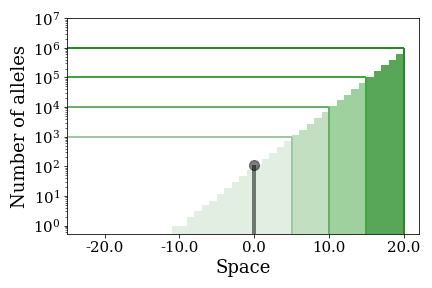
a1 $s=0.3$

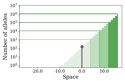
a2 $s=0.7$

(a) Initial conditions for the spatial Galton-Watson process, in shades of blue. The exponential profile used to initiate the simulation is cropped at different population size on the right, from $10^{3}$ to $10^{8}$, to evaluate the impact of migration from dense to less dense areas. The black line with a circle at the top represents the last spatial site with more than $100$ individuals in the initial condition. We record the extinction time $T^{100}_{0\ \text{gw}}$ of this site, and run the simulation 500 times to obtain its statistical distribution. This distribution (multiplied by the speed $v_{\text{num}}$ to approximate distance $L^{100}_{1}$) is illustrated in Figure 14(b).

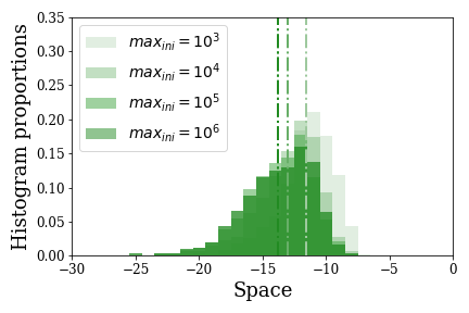
b1 $s=0.3$

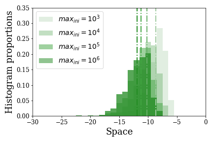
b2 $s=0.7$

(b) Statistical distribution of extinction time $T^{100}_{0\ \text{gw}}$, multiplied by the speed $v_{\text{num}}$ (to approximate distance $L^{100}_{1}$). We consider the initial conditions described in Figure 14(a) in shades of blue; each blue corresponds to a different space window in which the maximum number of individuals per site is $\max_{ini}$. We record the time $T^{100}_{0\ \text{gw}}$ at which the last spatial site with more than $100$ individuals in the initial condition goes extinct (definitively). The dashed lines are the means values of each histogram.

Figure 14: Initial conditions and extinction times for the isolated population.

Appendix D Comparison with the 2D case, small carrying capacity $K=10^{3}$

We run the same simulations than in Figure 10 except for the carrying capacity that is taken smaller $K=10^{3}$. For small drive fitness cost ($s=0.3$), the outcomes stays unchanged: we observe no wild-type recolonisation event and the drive propagation leads to the full eradication of the population both in 1D and 2D. For large drive fitness cost ($s=0.7$), we observe several wild-type recolonisation and drive reinvasion events, due to the small carrying capacity value (in comparison, we observe less stochastic events for $K=10^{5}$ in Figure 10(d)). The stochastic events appear to be more frequent in 2D than in 1D, similarly to what we observed for $K=10^{5}$ and $K=10^{8}$.

(a) $K=10^{3},s=0.3$

(b) $K=10^{3},s=0.7$

Figure 15: Comparison between the 1D and the 2D stochastic models for a small carrying capacity ($K=10^{3}$). Wild-type alleles are shown in blue and drive alleles in red. In 1D, the y-axis represents the number of alleles, while in 2D, the number of alleles is shown in shades of colour: the darker the colour, the more alleles of the corresponding type on the spatial site. For a small carrying capacity $s=0.3$, we observe no wild-type recolonisation events and the full eradication of the population in 1D and 2D, similarly to the numerical outcomes obtained with larger carrying capacity (Figure 10(a, b)). Note that the drive presence on the first half of the domain, in the earliest 1D snapshot of panel (a), is a simulation artefact due to the initial condition (Figure 3). For a large drive fitness cost $s=0.7$, reducing the carrying capacity results in a higher number of wild-type recolonisation and drive reinvasion events (in comparison with Figure 10(d)). Once again here, these stochastic events appear to be more frequent in 2D than in 1D.

Appendix E Exploring chasing dynamics

We test various values of intrinsic growth rate $r$ in order to appreciate its influence on the probability of drive reinvasion events after a wild-type recolonisation. Both the simulations in 1D (Figure 16) and the simulations in 2D (Figure 17) illustrate the concept described in Section 3.9: as $r$ increases, the wild-type recolonisation wave and the drive eradication wave get closer, increasing the probability to observe drive reinvasion events. In the following example, both the wild-type recolonisation probability ($p_{A}$) and the drive reinvasion probability ($p_{B}$) are high and relatively close for high values of $r$, which leads to infinite chasing dynamics (Figure 16(c) and 17(c)).

(a) $r=0.05$

(b) $r=0.1$

(c) $r=0.2$

Figure 16: Simulations in 1D for $K=10^{3}$ and $s=0.7$. As the value of $r$ increases, drive reinvasion events are more and more frequent.

(a) $r=0.02$

(b) $r=0.05$

(c) $r=0.1$

Figure 17: Simulations in 2D for $K=10^{2}$ and $s=0.3$. As the value of $r$ increases, drive reinvasion events are more and more frequent.

References

- [1] Nicolas O. Rode et al. “Population management using gene drive: molecular design, models of spread dynamics and assessment of ecological risks” In Conservation Genetics 20.4, 2019, pp. 671–690 DOI: 10.1007/s10592-019-01165-5
- [2] Austin Burt “Site-specific selfish genes as tools for the control and genetic engineering of natural populations.” In Proceedings of the Royal Society B: Biological Sciences 270.1518, 2003, pp. 921–928 DOI: 10.1098/rspb.2002.2319
- [3] Gernot Segelbacher et al. “New developments in the field of genomic technologies and their relevance to conservation management” In Conservation Genetics 23.2, 2022, pp. 217–242 DOI: 10.1007/s10592-021-01415-5
- [4] Luke S. Alphey, Andrea Crisanti, Filippo (Fil) Randazzo and Omar S. Akbari “Standardizing the definition of gene drive” Publisher: Proceedings of the National Academy of Sciences In Proceedings of the National Academy of Sciences 117.49, 2020, pp. 30864–30867 DOI: 10.1073/pnas.2020417117
- [5] Austin Burt and Andrea Crisanti “Gene Drive: Evolved and Synthetic” Publisher: American Chemical Society In ACS Chemical Biology 13.2, 2018, pp. 343–346 DOI: 10.1021/acschembio.7b01031
- [6] Ethan Bier “Gene drives gaining speed” In Nature Reviews Genetics 23.1 Nature Publishing Group UK London, 2022, pp. 5–22
- [7] Kyros Kyrou et al. “A CRISPR–Cas9 gene drive targeting doublesex causes complete population suppression in caged Anopheles gambiae mosquitoes” Number: 11 Publisher: Nature Publishing Group In Nature Biotechnology 36.11, 2018, pp. 1062–1066 DOI: 10.1038/nbt.4245
- [8] Andrew Hammond et al. “Gene-drive suppression of mosquito populations in large cages as a bridge between lab and field” Number: 1 Publisher: Nature Publishing Group In Nature Communications 12.1, 2021, pp. 4589 DOI: 10.1038/s41467-021-24790-6
- [9] H. J. Godfray, Ace North and Austin Burt “How driving endonuclease genes can be used to combat pests and disease vectors” In BMC Biology 15.1, 2017, pp. 81 DOI: 10.1186/s12915-017-0420-4
- [10] Léo Girardin and Florence Débarre “Demographic feedbacks can hamper the spatial spread of a gene drive” In Journal of Mathematical Biology 83.6, 2021, pp. 67 DOI: 10.1007/s00285-021-01702-2
- [11] Ace R. North, Austin Burt and H. J. Godfray “Modelling the suppression of a malaria vector using a CRISPR-Cas9 gene drive to reduce female fertility” In BMC Biology 18, 2020, pp. 98 DOI: 10.1186/s12915-020-00834-z
- [12] Jackson Champer et al. “Suppression gene drive in continuous space can result in unstable persistence of both drive and wild-type alleles” In Molecular Ecology 30.4, 2021, pp. 1086–1101 DOI: 10.1111/mec.15788
- [13] James J Bull, Christopher H Remien and Stephen M Krone “Gene-drive-mediated extinction is thwarted by population structure and evolution of sib mating” In Evolution, Medicine, and Public Health 2019.1, 2019, pp. 66–81 DOI: 10.1093/emph/eoz014
- [14] Ace R. North, Austin Burt and H. J. Godfray “Modelling the potential of genetic control of malaria mosquitoes at national scale” In BMC Biology 17.1, 2019, pp. 26 DOI: 10.1186/s12915-019-0645-5
- [15] Aysegul Birand et al. “Gene drives for vertebrate pest control: Realistic spatial modelling of eradication probabilities and times for island mouse populations” In Molecular Ecology 31.6, 2022, pp. 1907–1923 DOI: 10.1111/mec.16361
- [16] Samuel E Champer et al. “Anopheles homing suppression drive candidates exhibit unexpected performance differences in simulations with spatial structure” Publisher: eLife Sciences Publications, Ltd In eLife 11, 2022, pp. e79121 DOI: 10.7554/eLife.79121
- [17] Yiran Liu, WeiJian Teo, Haochen Yang and Jackson Champer “Adversarial interspecies relationships facilitate population suppression by gene drive in spatially explicit models” In Ecology Letters 26.7, 2023, pp. 1174–1185 DOI: 10.1111/ele.14232
- [18] Yiran Liu and Jackson Champer “Modelling homing suppression gene drive in haplodiploid organisms” Publisher: Royal Society In Proceedings of the Royal Society B: Biological Sciences 289.1972, 2022, pp. 20220320 DOI: 10.1098/rspb.2022.0320
- [19] Jeff F. Paril and Ben L. Phillips “Slow and steady wins the race: spatial and stochastic processes and the failure of suppression gene drives” In Molecular Ecology, 2022, pp. mec.16598 DOI: 10.1111/mec.16598
- [20] Yutong Zhu and Jackson Champer “Simulations Reveal High Efficiency and Confinement of a Population Suppression CRISPR Toxin-Antidote Gene Drive” Publisher: American Chemical Society In ACS Synthetic Biology 12.3, 2023, pp. 809–819 DOI: 10.1021/acssynbio.2c00611
- [21] Léna Kläy, Léo Girardin, Vincent Calvez and Florence Débarre “Pulled, pushed or failed: the demographic impact of a gene drive can change the nature of its spatial spread” In Journal of Mathematical Biology 87.2, 2023, pp. 30 DOI: 10.1007/s00285-023-01926-4
- [22] James D Murray “Mathematical biology: I. An introduction” Springer Science & Business Media, 2007
- [23] Eric Brunet and Bernard Derrida “Shift in the velocity of a front due to a cutoff” Publisher: American Physical Society In Physical Review E 56.3, 1997, pp. 2597–2604 DOI: 10.1103/PhysRevE.56.2597
- [24] Éric Brunet and Bernard Derrida “Effect of Microscopic Noise on Front Propagation” In Journal of Statistical Physics 103.1, 2001, pp. 269–282 DOI: 10.1023/A:1004875804376
- [25] Jean Bérard and Jean-Baptiste Gouéré “Brunet-Derrida Behavior of Branching-Selection Particle Systems on the Line” In Communications in Mathematical Physics 298.2, 2010, pp. 323–342 DOI: 10.1007/s00220-010-1067-y
- [26] Carl Mueller, Leonid Mytnik and Jeremy Quastel “Effect of noise on front propagation in reaction-diffusion equations of KPP type” In Inventiones mathematicae 184.2, 2011, pp. 405–453 DOI: 10.1007/s00222-010-0292-5
- [27] Daniela Bertacchi and Fabio Zucca “Recent results on branching random walks” arXiv, 2018 DOI: 10.48550/arXiv.1104.5085
- [28] R.. Fisher “The Wave of Advance of Advantageous Genes” _eprint: https://onlinelibrary.wiley.com/doi/pdf/10.1111/j.1469-1809.1937.tb02153.x In Annals of Eugenics 7.4, 1937, pp. 355–369 DOI: 10.1111/j.1469-1809.1937.tb02153.x
- [29] Jason W. Chapman, V. Drake and Don R. Reynolds “Recent Insights from Radar Studies of Insect Flight” _eprint: https://doi.org/10.1146/annurev-ento-120709-144820 In Annual Review of Entomology 56.1, 2011, pp. 337–356 DOI: 10.1146/annurev-ento-120709-144820
- [30] Gao Hu et al. “Mass seasonal bioflows of high-flying insect migrants” Publisher: American Association for the Advancement of Science In Science 354.6319, 2016, pp. 1584–1587 DOI: 10.1126/science.aah4379
- [31] Diana L. Huestis et al. “Windborne long-distance migration of malaria mosquitoes in the Sahel” Number: 7778 Publisher: Nature Publishing Group In Nature 574.7778, 2019, pp. 404–408 DOI: 10.1038/s41586-019-1622-4
- [32] Andrea Egizi, Jay Kiser, Charles Abadam and Dina M. Fonseca “The hitchhiker’s guide to becoming invasive: exotic mosquitoes spread across a US state by human transport not autonomous flight” _eprint: https://onlinelibrary.wiley.com/doi/pdf/10.1111/mec.13653 In Molecular Ecology 25.13, 2016, pp. 3033–3047 DOI: 10.1111/mec.13653
- [33] Roger Eritja et al. “Direct Evidence of Adult Aedes albopictus Dispersal by Car” In Scientific Reports 7.1, 2017, pp. 14399 DOI: 10.1038/s41598-017-12652-5
- [34] Andrea K. Beaghton et al. “Gene drive for population genetic control: non-functional resistance and parental effects” Publisher: Royal Society In Proceedings of the Royal Society B: Biological Sciences 286.1914, 2019, pp. 20191586 DOI: 10.1098/rspb.2019.1586
- [35] Andrew M. Hammond et al. “The creation and selection of mutations resistant to a gene drive over multiple generations in the malaria mosquito” Publisher: Public Library of Science In PLOS Genetics 13.10, 2017, pp. e1007039 DOI: 10.1371/journal.pgen.1007039
- [36] Tom A.. Price et al. “Resistance to natural and synthetic gene drive systems” In Journal of Evolutionary Biology 33.10, 2020, pp. 1345–1360 DOI: 10.1111/jeb.13693