Learning-Driven Annealing with Adaptive Hamiltonian Modification for Solving Large-Scale Problems on Quantum Devices

Sebastian Schulz Thanks: Corresponding author: Sebastian Schulz Email: se.schulz@fz-juelich.de Affiliation: Jülich Supercomputing Centre, Institute for Advanced Simulation,
Forschungszentrum Jülich, 52425 Jülich, Germany
   Dennis Willsch Affiliation: Jülich Supercomputing Centre, Institute for Advanced Simulation,
Forschungszentrum Jülich, 52425 Jülich, Germany
Affiliation: Faculty of Medical Engineering and Technomathematics, University of Applied Sciences Aachen,
52428 Jülich, Germany
   Kristel Michielsen Affiliation: Jülich Supercomputing Centre, Institute for Advanced Simulation,
Forschungszentrum Jülich, 52425 Jülich, Germany
Affiliation: AIDAS, 52425 Jülich, Germany Affiliation: RWTH Aachen University, 52056 Aachen, Germany
August 9, 2026
Abstract

We present Learning-Driven Annealing (LDA), a framework that links individual quantum annealing evolutions into a global solution strategy to mitigate hardware constraints such as short annealing times and integrated control errors. Unlike other iterative methods, LDA does not tune the annealing procedure (e.g. annealing time or annealing schedule), but instead learns about the problem structure to adaptively modify the problem Hamiltonian. By deforming the instantaneous energy spectrum, LDA suppresses transitions into high-energy states and focuses the evolution into low-energy regions of the Hilbert space. We demonstrate the efficacy of LDA by developing a hybrid quantum-classical solver for large-scale spin glasses. The hybrid solver is based on a comprehensive study of the internal structure of spin glasses, outperforming other quantum and classical algorithms (e.g., reverse annealing, cyclic annealing, simulated annealing, Gurobi, Toshiba’s SBM, VeloxQ and D-Wave hybrid) on 55805580-qubit problem instances in both runtime and lowest energy. LDA is a step towards practical quantum computation that enables today’s quantum devices to compete with classical solvers.

Keywords: 
Quantum computing, Quantum annealing, Learning-driven annealing, Feature Hamiltonian, Hybrid quantum-classical optimization, Spin glass

I Introduction

Combinatorial optimization problems (COPs) are ubiquitous in computer science, with important applications in finance Marzec 2016, scheduling Willsch et al. 2022a, machine learning Amin et al. 2018; Benedetti et al. 2016, computational biology Perdomo-Ortiz et al. 2012, and operations research Boucherie et al. 2021. For many such problems, finding the optimal solution is equivalent to finding the ground state of an associated Ising spin-glass system Lucas 2014. The hardness of COPs is related to the presence of opposing spin interactions, leading to frustration and a glass phase. The latter is characterized by the presence of many low-energy local minima, that are separated by large energy barriers. This makes solving large-scale COPs often intractable on classical computers, quickly exceeding runtimes of 2424 hours.

With the advent of new generations of quantum annealers from D-Wave Systems Inc. comprising more than 50005000 qubits, a promising approach is the use of quantum annealing (QA) Yarkoni et al. 2022; King et al. 2024; Pelofske 2025. Inspired by the cooling of physical systems, QA uses quantum fluctuations caused by a transverse field to navigate the energy landscape of the spin system Rajak et al. 2023. If the quantum evolution is performed adiabatically, the system arrives in the ground state of the spin glass. However, if the evolution is too fast, the system scatters into higher energy states through a series of quantum phase transitions (QPTs, used in the sense of Refs. Amin and Choi 2009; Schaller and Schützhold 2010; Schützhold and Schaller 2006; Nishimori and Ortiz 2015). Hence, on real devices, finite annealing times and integrated control errors limit the performance, often making deep low-energy states (including the ground state) inaccessible Altshuler et al. 2010; Villanueva et al. 2023. To address this issue, several authors recently investigated iterative procedures, such as reverse annealing Chancellor 2017; Yamashiro et al. 2019; Perdomo-Ortiz et al. 2011; Mehta et al. 2025a and cyclic annealing Wang et al. 2022; Zhang et al. 2024; Pelofske et al. 2023, in which the annealing is repeatedly initialized from the best known classical state. In doing so, the hope is that QA gradually converges to the ground state, but in practice, these procedures often fail, as they become stuck in high-energy valleys Chancellor and Kendon 2021; Passarelli et al. 2020.

We show that modifications to the problem Hamiltonian itself can greatly improve the performance of iterative QA on noisy hardware. With Learning-Driven Annealing (LDA), we propose a framework to link individual QA runs into a global solution strategy to mitigate hardware constraints such as finite annealing times and integrated control errors D-Wave Systems Inc. 2025a. LDA works by analyzing the states sampled from QA to adaptively modify the problem Hamiltonian to the information learned about the energy landscape. This energetically isolates low-energy valleys in the instantaneous energy spectrum, focussing subsequent annealing runs into a promising region of the Hilbert space. As a result, the QPU can reach deeper regions of the energy spectrum that are otherwise inaccessible, enabling NISQ devices to tackle any COP that can be embedded onto their hardware.

We demonstrate the capabilities of LDA by designing a hybrid quantum-classical solver for large-scale spin glasses, that is based on alternating local and global search protocols. Using the D-Wave Advantage 5.4 QPU QPU 2025 in Jülich, Germany, we benchmark our hybrid solver against leading quantum and classical algorithms, including reverse annealing Chancellor 2017, cyclic annealing Wang et al. 2022; Zhang et al. 2024, simulated annealing using JUPTSA Hans De Raedt 2024, Gurobi Gurobi Optimization, LLC 2024, Toshiba’s SBM Toshiba Digital Solutions Corporation 2025, VeloxQ Pawłowski et al. 2025 and D-Wave hybrid D-Wave Systems Inc. 2025b, on 55805580-qubit NAT-7 Katzgraber et al. 2014; McGeoch and Farré 2024 spin glasses. The results show that our hybrid solver outperforms all competing strategies in both runtime and lowest energy. LDA is a step towards practical quantum computation that enables today’s quantum annealers to compete with classical solvers.

The remainder of this paper is organized as follows: In Sec. II, we introduce the spin-glass formulation and provide insights into its underlying structures. Section III concerns adiabatic quantum evolutions and discusses its limitations on modern quantum annealers. In Sec. IV, we introduce the LDA framework, showcasing how learned information from sampled states can be used to guide the annealing evolution by modifying the problem Hamiltonian. In Sec. V, we demonstrate how LDA can be used in advanced algorithms by designing a hybrid solver for spin glasses based on alternating local and global search protocols. Finally, in Sec. VI, we benchmark our hybrid solver against various classical and quantum solvers, followed by a summary of our findings in Sec. VII.

Refer to caption
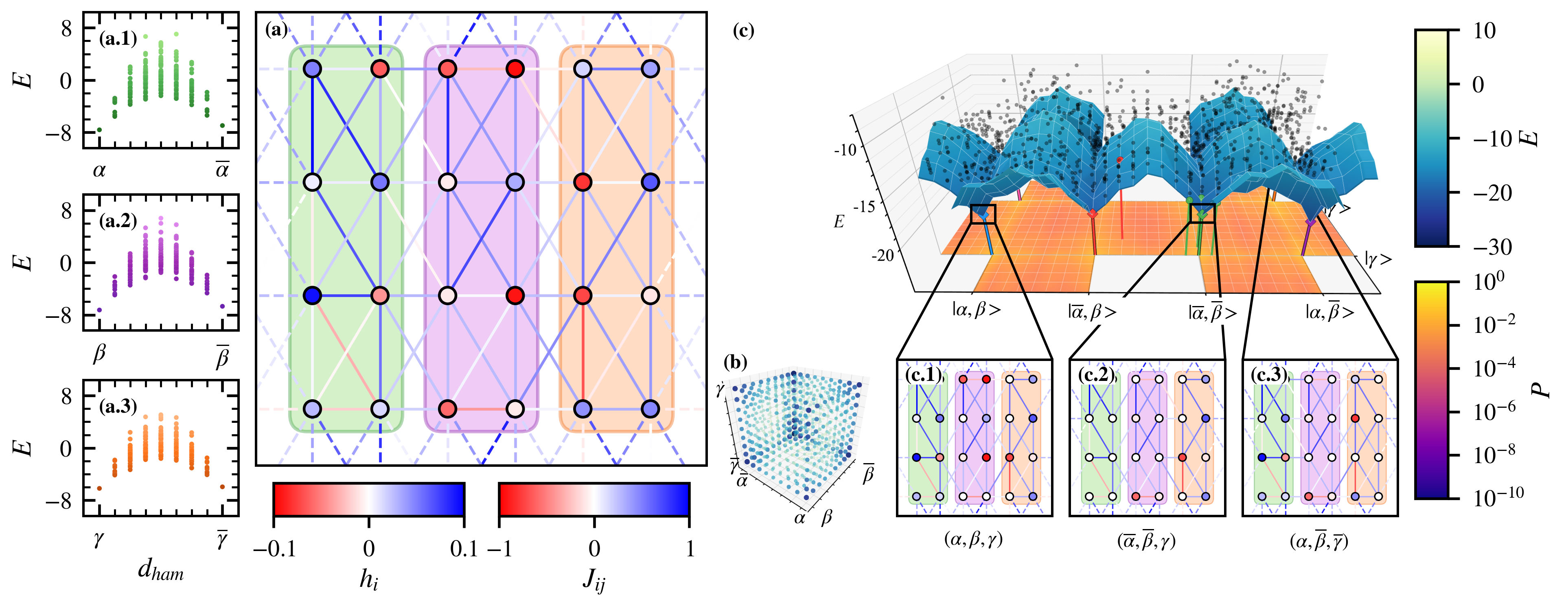
Figure 1: A 2424-qubit spin-glass with Ndom=3N_{dom}=3. (a) Spin-glass graph with the biases hih_{i} as nodes and couplers JijJ_{ij} as edges. Dashed edges indicate periodic boundary conditions. The colored rectangles represent the spin domains: 𝒟1\mathcal{D}_{1} (green), 𝒟2\mathcal{D}_{2} (purple), and 𝒟3\mathcal{D}_{3} (orange). Each domain has two distinct minima: α\alpha and α¯\overline{\alpha} (𝒟1\mathcal{D}_{1}), β\beta and β¯\overline{\beta} (𝒟2\mathcal{D}_{2}), γ\gamma and γ¯\overline{\gamma} (𝒟3\mathcal{D}_{3}). Panels (a.1-3) show the eigenenergies EE of the corresponding domains as a function of the Hamming distance dhamd_{ham} to the respective ground state α,β,γ\alpha,\beta,\gamma. (b) Hypercube representation of the Hilbert space, with each axis representing the Hamming distance dhamd_{ham} from the ground state (α,β,γ\alpha,\beta,\gamma) of the respective spin domains 𝒟k\mathcal{D}_{k}. Color indicates the lowest eigenenergy at each point. The corners of the hypercube correspond to the 2Ndom=82^{N_{dom}}=8 local minima of the spin glass. (c) Energy landscape of the spin glass obtained by unfolding the hypercube facets. Each point is projected onto the closest facet (smallest Hamming distance), with the blue surface representing the lowest eigenenergies on these facets. The eight local minima are marked by colored diamonds at the facets’ corners, with the states surrounding it being the energy valleys. Additionally, black dots indicate 20002000 samples from a quantum annealing simulation with annealing time T=10T=10, with the probability density shown on the lower orange plane. Panels (c.1-3) highlight the specific biases hih_{i} and couplers JijJ_{ij} satisfied by three of the eight local minima, with the unsatisfied terms set to 00 (white). The color scheme matches that of panel (a).

II Spin-glass problems

Spin glasses (SG) are magnetic systems of quenched disorder, imposing conflicts between interacting magnetic moments Binder and Young 1986. In the Edwards-Anderson model of SG Edwards and Anderson 1975, NN Ising spins σiz\sigma^{z}_{i}, i{0,,N1}i\in\{0,\,\dots\,,\,N-1\}, are placed on the sites of a regular graph, with the Hamiltonian defined as

H=i<jJijσizσjz+ihiσiz.\displaystyle H=\sum_{i<j}J_{ij}\sigma^{z}_{i}\sigma^{z}_{j}+\sum_{i}h_{i}\sigma^{z}_{i}. (1)

Here JijJ_{ij} with i<ji<j denotes the coupling strength between spins ii and jj, and hih_{i} represents a locally applied external magnetic field bias on spin ii.

We consider both triangular lattices with periodic boundary conditions (see Fig. 1a) and the Pegasus graph used by the D-Wave Advantage 5.4 quantum annealer QPU 2025. In the following, we choose |hi||Jij|\lvert h_{i}\rvert\ll\lvert J_{ij}\rvert to ensure the generation of complex SG Katzgraber et al. 2015. Notably, for hi=0h_{i}=0, HH exhibits a global 2\mathbb{Z}_{2} symmetry.

Throughout this study, we use Greek letters, e.g. α=αN1α1α0\alpha=\alpha_{N-1}\cdots\alpha_{1}\alpha_{0}, to represent a generic eigenstate of Eq. (1), with αi=±1\alpha_{i}=\pm 1 denoting the polarization of the ii-th spin. We also use the notation α=αN1α1α0\alpha^{*}=\alpha_{N-1}^{*}\cdots\alpha_{1}^{*}\alpha_{0}^{*} to refer to a local (in Hamming distance) minimum of Eq. (1). The eigenenergy of a state α\alpha is given by Eα=i<jJijαiαj+ihiαiE_{\alpha}=\sum_{i<j}J_{ij}\alpha_{i}\alpha_{j}+\sum_{i}h_{i}\alpha_{i} and its bit string representation is written as a=aN1a1a0\texttt{a}=\texttt{a}_{N-1}\cdots\texttt{a}_{1}\texttt{a}_{0}, with ai=(1+αi)/2\texttt{a}_{i}=(1+\alpha_{i})/2.

For a given state α\alpha, we define the set of satisfied (i.e., non-frustrated) couplers and biases as

𝒥α\displaystyle\mathcal{J}^{\alpha} ={(i,j)Jijαiαj<0},\displaystyle=\{(i,j)\mid J_{ij}\alpha_{i}\alpha_{j}<0\}, (2a)
α\displaystyle\mathcal{H}^{\alpha} ={ihiαi<0}.\displaystyle=\{i\mid h_{i}\alpha_{i}<0\}. (2b)

These sets consist of those couplings and biases of Eq. (1) that are satisfied in the state α\alpha, meaning that the corresponding terms in the Hamiltonian contribute to a reduction of the total energy of the system.

Intuitively, the presence of competing spin-spin interactions in Eq. (1) causes frustration, which prevents the ground state from establishing a simple long-range (anti-)ferromagnetic order. Instead, the spins align in random directions, forming a glass phase Stein and Newman 2011. This phase is characterized by the existence of exponentially many low-energy local minima, where a local minimum refers to a state for which flipping a single (or a few) spins always increases the energy. The energy spectrum of these local minima typically has small gaps, with macroscopic high and wide energy barriers separating them Mukherjee and Chakrabarti 2019. The latter implies that 𝒪(N)\mathcal{O}(N) spins would need to be flipped in order to escape a local minimum Binder and Young 1986. Despite the complexity of the energy landscape, the formation of local minima stems from a general structure in the interactions of the spins. Local differences in the spin-spin couplings and biases lead to the formation of spin domains 𝒟1,,𝒟Ndom{0,,N1}\mathcal{D}_{1},\,\dots\,,\,\mathcal{D}_{N_{\mathrm{dom}}}\subset\{0,\,\dots\,,\,N-1\}, representing groups of highly correlated spins Binder and Young 1986; Amin 2008.

II.1 Spin domains

We define a spin domain 𝒟k{0,,N1}\mathcal{D}_{k}\subset\{0,\,\dots\,,\,N-1\}, with k=1,,Ndomk=1,\,\dots\,,\,N_{\mathrm{dom}}, as a maximally large connected sub-spin glass of Eq. (1), such that its energy landscape is ergodic with respect to spin-reversal transformations. This means that the ground state of the domain is accessible from any state through a sequence of decreasing energies using solely single spin flips and state inversions (i.e. flipping all spins). In computational terms, ergodic means that the global minimum of the domain can be reached via a greedy search algorithm. Note that a domain can consist of a single spin if the local magnetic field hih_{i} dominates the interaction. An example 2424-qubit spin glass with Ndom=3N_{\mathrm{dom}}=3 domains is shown in Fig. 1a. The respective energy spectra of the spin domains are given in panels (a.1-3).

Each spin domain 𝒟k\mathcal{D}_{k} identifies a trivial sub-spin glass, defined by the quadratic terms i,j𝒟ki,j\in\mathcal{D}_{k} within the domain,

i,j𝒟kJijσizσjz.\displaystyle\sum_{i,j\in\mathcal{D}_{k}}J_{ij}\sigma_{i}^{z}\sigma_{j}^{z}. (3)

This sub-spin glass has two degenerate ground states β(k)\beta^{*(k)} and β(k)¯\overline{\beta^{*(k)}}, due to the 2\mathbb{Z}_{2} symmetry of the spin-spin couplers, with β(k)¯\overline{\beta^{*(k)}} denoting the inverse state of β(k)\beta^{*(k)} (i.e., all spins flipped). By combining the ground states of all domains, the 2Ndom2^{N_{\mathrm{dom}}} local minima of the full spin glass can be constructed. Consequently, these local minima form an NdomN_{\mathrm{dom}}-dimensional hypercube, with the edges denoting state inversions of single spin domains (see Fig. 1b).

The complexity of the spin-glass energy landscape stems from the domain borders, where spin domains couple to each other (i.e. spin-spin couplings JijJ_{ij} between domains) and to the local biases hih_{i}. These interactions lift the degeneracies of the domains’ ground states, assigning energy shifts to the local minima and forming a hierarchy on the hypercube Hed et al. 2001.

For the three-dimensional hypercube shown in Fig. 1b, Fig. 1c visualizes the energy landscape obtained by unfolding its facets. Note that the hardness of spin glasses arises from the lack of knowledge about the exact domains 𝒟k\mathcal{D}_{k}. If the distribution of spin domains were known, the complexity of the problem would be reduced from 2N2^{N} to 2Ndom2^{N_{dom}} with the number of domains NdomNN_{dom}\ll N.

II.2 Distance measures

For the following description of LDA, a distance measure between arbitrary spin configurations α\alpha and β\beta is required. A commonly used metric for this purpose is the Edward-Anderson order parameter Edwards and Anderson 1975, measuring the overlap of the states α\alpha and β\beta as

qEA(α,β)=1Ni=0N1αiβi.\displaystyle q_{EA}(\alpha,\beta)=\frac{1}{N}\sum^{N-1}_{i=0}\alpha_{i}\beta_{i}. (4)

By definition, qEA[1,1]q_{EA}\in[-1,1], with qEA=1α=βq_{EA}=1\Leftrightarrow\alpha=\beta and qEA=1α=β¯q_{EA}=-1\Leftrightarrow\alpha=\overline{\beta}. Note that qEAq_{EA} is directly related to the Hamming distance dhamd_{\mathrm{ham}} between the bit strings a and b via dham=N(1qEA)/2d_{\mathrm{ham}}=N(1-q_{EA})/2.

While qEAq_{EA} is a sufficient tool for the statistical analysis of phase transitions in disordered systems King et al. 2023, it is indifferent to the distance between the energies EαE_{\alpha} and EβE_{\beta} of the states. This means that two states with the same order parameter qEAq_{EA} can have significantly different energies, depending on the amount of frustration that they cause. To compensate for this, we propose a quantity qF(α,β)q_{F}(\alpha,\beta) that evaluates the similarity between a reference state α\alpha and a state β\beta based on the sets of simultaneously satisfied couplers 𝒥α𝒥β\mathcal{J}^{\alpha}\cap\mathcal{J}^{\beta} and biases αβ\mathcal{H}^{\alpha}\cap\mathcal{H}^{\beta} (see Eq. (2)), defined as

qF(α,β)=(i,j)𝒥α𝒥βwith(αi,αj)=(βi,βj)|Jij|+iαβ|hi|(i,j)𝒥α|Jij|+iα|hi|.\displaystyle q_{F}(\alpha,\beta)=\frac{\sum\limits_{\begin{subarray}{c}(i,j)\in\mathcal{J}^{\alpha}\cap\mathcal{J}^{\beta}\\ \mathrm{with}\>(\alpha_{i},\alpha_{j})=(\beta_{i},\beta_{j})\end{subarray}}|J_{ij}|+\sum\limits_{i\in\mathcal{H}^{\alpha}\cap\mathcal{H}^{\beta}}|h_{i}|}{\sum\limits_{(i,j)\in\mathcal{J}^{\alpha}}|J_{ij}|+\sum\limits_{i\in\mathcal{H}^{\alpha}}|h_{i}|}. (5)

By definition, qF[0,1]q_{F}\in[0,1], with qF=1(0)q_{F}=1\;(0) denoting that βα\mathcal{H}^{\beta}\subset\mathcal{H}^{\alpha} (βα=)\left(\mathcal{H}^{\beta}\cap\mathcal{H}^{\alpha}=\emptyset\right) and 𝒥β𝒥α\mathcal{J}^{\beta}\subset\mathcal{J}^{\alpha} (𝒥β𝒥α=)\left(\mathcal{J}^{\beta}\cap\mathcal{J}^{\alpha}=\emptyset\right). We remark that in the singular case α=𝒥α=\mathcal{H}^{\alpha}=\mathcal{J}^{\alpha}=\emptyset, we define qF=1q_{F}=1. The additional condition αi=βi\alpha_{i}=\beta_{i} in the first summation of Eq. (5) ensures that the spins in the simultaneously satisfied couplers JijJ_{ij} are also aligned with one another, (αi,αj)=(βi,βj)(\alpha_{i},\alpha_{j})=(\beta_{i},\beta_{j}). This is necessary because Jijαiαj=Jijβiβj<0J_{ij}\alpha_{i}\alpha_{j}=J_{ij}\beta_{i}\beta_{j}<0 would also be satisfied if (αi,αj)=(βi¯,βj¯)(\alpha_{i},\alpha_{j})=(\overline{\beta_{i}},\overline{\beta_{j}}). Hence, the condition lifts the spin-reversal symmetry of the spin domains, in order to account for the Hamming distance between the states.

Refer to caption
Figure 2: Comparison of the quanitiy qF(α,β)q_{F}(\alpha^{*},\beta) to (a) the Edward-Anderson order parameter qEA(α,β)q_{EA}(\alpha^{*},\beta) and (b) the energy difference ΔE=EβEα\Delta E=E_{\beta}-E_{\alpha^{*}} for states β\beta w.r.t. the global minimum α\alpha^{*} of the 2424-qubit spin-glass shown in Fig. 1a. The colored diamonds mark the eight local minima (see Fig. 1c).

The definition of qFq_{F} is based on the observation that each local minimum α\alpha^{*} can be uniquely identified (up to state inversion in case of hi=0h_{i}=0) by the sets of satisfied couplers 𝒥α\mathcal{J}^{\alpha^{*}} and biases α\mathcal{H}^{\alpha^{*}} (see Fig. 1c.1-3, where the local minima satisfy different couplers between the domains). By ranking each state according to its energy in the sub spin-glass (𝒥α,α)\left(\mathcal{J}^{\alpha^{*}},\,\mathcal{H}^{\alpha^{*}}\right), the parameter qFq_{F} integrates both the Hamming distance (qEAq_{EA}) and the energy distance (ΔE\Delta E) from α\alpha^{*} into the similarity measure (see Fig. 2a). This allows qFq_{F} to distinguish the energy valley of α\alpha^{*} (i.e. the neighborhood of states around α\alpha^{*}, where some domains are in an excited state) from the other local minima in Fig. 1c. As a result, only states with both a small Hamming distance and energy distance are considered close to α\alpha^{*}, making qFq_{F} indifferent to low-energy states of other energy valleys (see peaks at ΔE0\Delta E\approx 0 in Fig. 2b).

A key property of qFq_{F} is its asymmetry (i.e. qF(α,β)qF(β,α)q_{F}(\alpha,\beta)\neq q_{F}(\beta,\alpha)), since Eq. (5) considers only terms that are satisfied by the reference state α\alpha, but ignores additional terms satisfied by β\beta. As a consequence, a state β\beta deeper in the energy valley, with 𝒥β𝒥α\mathcal{J}^{\beta}\supset\mathcal{J}^{\alpha} and βα\mathcal{H}^{\beta}\supset\mathcal{H}^{\alpha}, typically has a larger qFq_{F} value than a higher-energy state, which violates terms in α\mathcal{H}^{\alpha} and 𝒥α\mathcal{J}^{\alpha}. This means that qFq_{F} has an intrinsic bias towards lower-energy states, which will be crucial for the definition of LDA in Sec. IV.

III Adiabatic quantum annealing

Adiabatic quantum annealing, as proposed by Farhi et al. Farhi et al. 2000, is a procedure for solving NP-hard combinatorial optimization problems (COP) through quantum fluctuations. With the search space of the COP encoded in the eigenspectrum of a problem Hamiltonian HPH_{P} (e.g. Eq. (1)), the system is complemented by a driving Hamiltonian HDH_{D} that is non-diagonal in the eigenbasis of HPH_{P}. Since the spin-glass Hamiltonian Eq. (1) is diagonal in the computational basis, we consider the transverse field Ising model

HQA(t)=HP+Γ(t)HDwithHD=i=0N1σix,\displaystyle H_{QA}(t)=H_{P}+\Gamma(t)\cdot H_{D}\;\;\text{with}\;\;H_{D}=-\sum^{N-1}_{i=0}\sigma^{x}_{i}, (6)

which is closely related to the design of D-Wave quantum annealers (see App. A). Γ(t)\Gamma(t) is the annealing schedule, defining the relative strength between HPH_{P} and HDH_{D} over time 0tT0\leq t\leq T. Initially, Γ(t=0)J\Gamma(t=0)\gg J, such that the instantaneous ground state (GS) is approximately given by |+N\ket{+}^{\bigotimes N} (where |+=(|0+|1)/2\ket{+}=(\ket{0}+\ket{1})/\sqrt{2}), which is initially separated by a large energy gap Γ(0)\propto\Gamma(0) from the rest of the spectrum. Operating the system at a temperature that is much smaller than the scale set by Γ(0)\Gamma(0) is supposed to initialize it in the GS of HDH_{D}. To reach the GS of HPH_{P}, Γ(t)\Gamma(t) is decreased adiabatically to zero as tTt\to T, allowing the system to follow the instantaneous GS of HQA(t)H_{QA}(t) Farhi et al. 2000; Albash and Lidar 2018a. In order to prevent Landau-Zener transitions into excited states during this process, the adiabatic theorem requires T1Δmin2T^{-1}\ll\Delta^{2}_{min} Amin 2009, where Δmin\Delta_{min} denotes the minimal energy gap between the two lowest instantaneous eigenstates of HQA(t)H_{QA}(t).

Refer to caption
Figure 3: (a) Instantaneous energy spectrum of the transverse field Ising model (see Eq. (6)) for the 2424-qubit spin-glass instance shown in Fig. 1a, using a linear annealing schedule Γ(t)\Gamma(t). The plot presents a selection of energy levels corresponding to the 88 valleys in the energy landscape (see Fig. 1c). For each valley, the local minimum (solid lines) is shown along with three states at Hamming distance dham=1d_{ham}=1 (dashed line) and three states at dham=2d_{ham}=2 (dash-dotted lines), representing the lowest-energy states along the edges of the hypercube. (b) Adiabatic ratios (see Eq. (7)) for the states presented in panel (a). The 24-qubit eigenstates and eigenvalues in the vicinity of each local minimum were obtained numerically by solving the time-dependent Schrödinger equation (see e.g. Willsch et al. 2022b) for reverse-annealing starting in the given states.

The minimum annealing time TT is the main measure for the computational complexity of adiabatic quantum annealing. Significant evidence exists that the presence of first-order quantum phase transitions (QPTs) during the adiabatic evolution causes an exponentially fast closure of Δmin\Delta_{min} with the system size NN, resulting in exponentially long annealing times Amin and Choi 2009; Schaller and Schützhold 2010. The authors in Amin 2008 argue that Δmin\Delta_{min} scales inversely proportional to the square root of the number of competing local minima (and states near them) with energies close to the global minimum and a large Hamming distances dhamd_{\mathrm{ham}}. Regarding the spin-glass instances under investigation, the number of local minima scales exponentially, 2Ndom2^{N_{\mathrm{dom}}}, with the number of domains NdomNN_{\mathrm{dom}}\propto N.

Figure 3a presents the instantaneous energy spectrum of the 2424-qubit spin-glass instance shown in Fig. 1a, with the adiabatic ratio Mori et al. 2024

g(t)=|m(t)|H˙QA(t)|GS(t)||Em(t)EGS(t)|2\displaystyle g(t)=\frac{\lvert\bra{m(t)}\dot{H}_{QA}(t)\ket{GS(t)}\rvert}{\lvert E_{m}(t)-E_{GS}(t)\rvert^{2}} (7)

depicted in Fig. 3b for the states marked in Fig. 1c. Here, |m(t)\ket{m(t)} (|GS(t)\ket{GS(t)}) denotes the instantaneous mm-th excited (ground) state, H˙QA(t)\dot{H}_{QA}(t) is the tt derivative of the instantaneous Hamiltonian and Em(t)E_{m}(t) (EGS(t)E_{GS}(t)) corresponds to the eigenenergies of the mm-th excited (ground) state.

In agreement with Schützhold and Schaller 2006; Albash and Lidar 2018b, the system undergoes a second-order QPTs at tc/T0.45t_{c}/T\approx 0.45, by evolving from the paramagnetic phase (localized in the σx\sigma_{x} basis) to an ordered phase (localized in the σz\sigma_{z} basis). As a result, the instantaneous eigenstates become semi-localized within energy valleys, forming superpositions of computational states within each valley Amin and Choi 2009. During the QPT, these valleys are coupled, as indicated by the peaks in gg for the 88 global and local minima (see solid lines in Fig. 3b). Additionally, the instantaneous energy spectrum exhibits transitions between states within the same valley. Since these states differ by small Hamming distances, they remain coupled after the second-order QPTs for t>tct>t_{c} (see blue dashed and dashed-dotted curves in Fig. 3b).

While the second-order QPT is generally associated with a polynomial scaling of TT, the presence of additional anti-crossings at t>tct>t_{c} between semi-localized states in large spin-glass instances induces first-order QPTs Amin and Choi 2009; Albash and Lidar 2018b. These transitions are characterized by energy gaps Δ\Delta that close exponentially with system size NN, leading to an exponential scaling of TT Schaller and Schützhold 2010; Schützhold and Schaller 2006. Recently, locally optimized annealing procedures have been proposed, which reduce TT by decelerating Γ(t)\Gamma(t) at the vicinity of the QPT Roland and Cerf 2002; Susa et al. 2018. However, these strategies can only provide a quadratic speedup Amin 2008. Since the required annealing times still exceed the accessible range on real devices, it is in practice impossible to solve large spin glasses using a single annealing run.

To overcome this bottleneck, several authors proposed the use of iterative protocols to incorporate classical information about the ground state into the annealing process Wang et al. 2022; Pelofske et al. 2023; Perdomo-Ortiz et al. 2011. The reverse annealing protocol, as proposed by Chancellor Chancellor 2017 and Yamashiro et al. Yamashiro et al. 2019, has been implemented on D-Wave QPUs. It starts by initializing the system in a computational basis state (e.g. obtained by a previous anneal or a classical heuristic), with Γ=0\Gamma=0. Quantum fluctuations are slowly introduced by increasing Γ\Gamma to an intermediate value Γ~\tilde{\Gamma} at t=Tst=T_{s}, where the process is paused for a period τ\tau until t=Tet=T_{e}. The protocol finishes by annealing back to Γ=0\Gamma=0 and measuring the qubits. By repeating this cycle and initializing each reverse anneal by the measurement of the previous, iterative reverse annealing (IRA) is hoped to move the system closer to the true ground state and overcome the above-mentioned limitation of an exponential annealing time TT.

In practice, however, reverse annealing performs a dissipative local search into the neighborhood of the initial state Chancellor and Kendon 2021. The spread of this search is controlled by the inversion point Γ~\tilde{\Gamma} and the QPTs it traverses. If no QPT is crossed, the system spreads locally (in Hamming distance) within its energy valley. However, if Γ~\tilde{\Gamma} is chosen large enough, such that a QPT is crossed, the system explores the search space globally by tunneling into other energy valleys Chancellor 2017. Note that TT must be sufficiently short, such that the process is non-adiabatic, because otherwise the system would simply return to its initial state.

In a closed system, there is no direct mechanism in the reverse annealing protocol to favor the search of lower-energy states Chancellor and Kendon 2021. Instead, the system spreads uniformly in energy around the initial state, gravitating (over multiple iterations) towards an equilibrium state, where the number of states with lower and higher energies balance. This makes it exponentially hard to find the ground state for N1N\gg 1.

On real devices, however, the QPU is always in interaction with its surrounding environment. In such open systems, thermal relaxation moderates the transition between neighboring states Mehta et al. 2025a; Mehta et al. 2025b. At sufficiently low temperatures, this causes a repopulation of lower-energy states during the pause, which allows reverse annealing to improve on the initial state. Passarelli et. al. Passarelli et al. 2020 argue that thermal relaxation is the main mechanism driving the performance of reverse annealing. This means that the success of IRA depends mainly on the effective temperature of the QPU. This gives an intuition as to why the D-Wave Advantage 5.45.4 QPU operating at 16.4mK\approx 16.4mK QPU 2025 is not able to find the ground state of the large spin glasses under investigation through IRA (see Sec. VI).

IV Learning-Driven Annealing

With Learning-Driven Annealing (LDA) we introduce a framework for linking individual QA runs into a global solution strategy to mitigate hardware limitations, such as finite annealing times and integrated control errors. LDA differs from other iterative strategies in that it does not tune the annealing procedure (e.g. annealing time or annealing schedule), but instead learns about the problem structure (i.e. spin domains) to systematically modify the problem Hamiltonian. LDA acts on the instantaneous energy spectrum in order to change the strength of QPTs between the energy valleys. This focuses the annealing evolution into a low-energy region of the Hilbert space by suppressing QPTs into high-energy valleys. LDA achieves this by replacing the problem Hamiltonian with a so-called feature Hamiltonian in the forward anneal. The construction of this Hamiltonian is based on the definition of the quantity qFq_{F} (see Eq. (5)) and adapts the strength of biases and couplers in HPH_{P} based on learned information about the domain structure to energetically isolate low-energy valleys in the instantaneous energy spectrum. This allows the annealing evolution to successively reach deeper states in the energy landscape.

Refer to caption
Figure 4: Construction of HFH_{F\mathcal{M}} (e, Eq. (15)) for the 2424-qubit spin-glass instance shown in Fig. 1, with λ=0.1\lambda=0.1. The feature Hamiltonian HFH_{F} (b) is derived from four sampled states (a.1-4) using Eq. (12) and the bitmask \mathcal{M}, with mi=1m_{i}=1 if the sampled states agree in the ii-th bit (this is the case for all non-white nodes shown in panel (b)). Panels (c) and (d) depict subsets of the original problem Hamiltonian, constructed using Eq. (14), with (c) applying to the terms included in HFH_{F}, and (d) addressing the remaining biases and couplers. Panels (b-e.1) illustrate the corresponding energy landscapes of the Hamiltonians in (b-e), with the four sampled states shown as black dots in (b.1).

The feature Hamiltonian, denoted as HF(α)H_{F}(\alpha), is defined w.r.t. a classical state α=αN1α1α0\alpha=\alpha_{N-1}\cdots\alpha_{1}\alpha_{0} for a spin glass instance P=(h,J)P=\left(h,J\right) as

HF(α)\displaystyle H_{F}(\alpha) =(i,j)𝒥αKij+iαhiσiz\displaystyle=\sum\limits_{(i,j)\in\mathcal{J}^{\alpha}}K_{ij}+\sum\limits_{i\in\mathcal{H}^{\alpha}}h_{i}\sigma^{z}_{i} (8)
Kij\displaystyle K_{ij} =|Jij|2[αiαjσizσjz+αiσiz+αjσjz].\displaystyle=-\frac{\lvert J_{ij}\rvert}{2}\left[\alpha_{i}\alpha_{j}\sigma^{z}_{i}\sigma^{z}_{j}+\alpha_{i}\sigma^{z}_{i}+\alpha_{j}\sigma^{z}_{j}\right]. (9)

α\mathcal{H}^{\alpha} and 𝒥α\mathcal{J}^{\alpha} denote the sets of satisfied biases and couplers, respectively (see Eq. (2b) and (2a)). HF(α)H_{F}(\alpha) transforms the energy spectrum of PP by retaining only terms that are satisfied by α\alpha in PP. This deforms the energy landscape according to the quantity qFq_{F} (see Eq. (5)), by arranging the states based on both their Hamming distance and energy distance from α\alpha, with α\alpha becoming the new ground state (see Thm. B.1).

In Eq. (8) we use the transformation JijσizσjzKijJ_{ij}\sigma_{i}^{z}\sigma_{j}^{z}\xrightarrow{}K_{ij} to lift the 2\mathbb{Z}_{2} symmetry of the spin-spin couplers JijJ_{ij} by introducing a penalty if either of the two spins ii and jj does not match the reference state α\alpha, i.e.,

Kij|αi,αj\displaystyle K_{ij}\ket{\alpha_{i},\alpha_{j}} =32|Jij|,Kij|αi,αj¯=12|Jij|\displaystyle=-\frac{3}{2}\lvert J_{ij}\rvert,\qquad K_{ij}\ket{\alpha_{i},\overline{\alpha_{j}}}=\frac{1}{2}\lvert J_{ij}\rvert (10)
Kij|αi¯,αj\displaystyle K_{ij}\ket{\overline{\alpha_{i}},\alpha_{j}} =12|Jij|,Kij|αi¯,αj¯=12|Jij|.\displaystyle=\frac{1}{2}\lvert J_{ij}\rvert,\qquad\;\;\;K_{ij}\ket{\overline{\alpha_{i}},\overline{\alpha_{j}}}=\frac{1}{2}\lvert J_{ij}\rvert. (11)

Note that the weighting of the biases hih_{i} and couplers JijJ_{ij} remains unchanged compared to the original problem Hamiltonian by using energy gaps of 2|hi|2\lvert h_{i}\rvert and 2|Jij|2\lvert J_{ij}\rvert, respectively. This transformation corresponds to the condition αi=βi\alpha_{i}=\beta_{i} in Eq. (5) and removes the degeneracy of the spin domains (i.e., each domain now has only one GS). Since the domain’s degeneracy is responsible for the existence of energy valleys (see Fig. 1c), removing the 2\mathbb{Z}_{2} symmetry flattens the energy landscape, while the restriction of HF(α)H_{F}(\alpha) to α\mathcal{H}^{\alpha} and 𝒥α\mathcal{J}^{\alpha} deforms the landscape in the direction of the reference state α\alpha (see Fig. 4b.1). As a result, the energy landscape becomes monotonic as a function of Hamming distance from α\alpha (see Thm. B.2 in App. B). Using a forward anneal, LDA explores the hypercube locally around α\alpha, with measurement probabilities scaling in the quantity qFq_{F}.

The exploration of the hypercube around α\alpha through LDA is based on the elements of α\mathcal{H}^{\alpha} and 𝒥α\mathcal{J}^{\alpha}, referred to as features, which energetically define the region of the hypercube where the annealing evolution concentrates. These features represent the extent of information provided by α\alpha regarding the location of a nearby local minimum α\alpha^{*}. If α\alpha is a high-energy state, most biases and couplers in PP are frustrated, leading to a highly degenerate HF(α)H_{F}(\alpha) with an almost flat energy landscape. In this case, the evolution spreads over large distances qFq_{F}, exploring the hypercube globally, as nearly any combination of spin flips reduces the system’s energy. This situation changes as α\alpha approaches a local minimum α\alpha^{*}. As the overlap between the sets of satisfied terms of α\alpha and α\alpha^{*} increases, HF(α)H_{F}(\alpha) incorporates more features that characterize the local minimum, resulting in an increasingly deformed energy landscape that focuses the evolution locally around α\alpha in the hypercube. Consequently, the search slows and becomes more fine-grained as LDA gains greater certainty about the location of a nearby local minimum.

Analogously to the asymmetry of the quantity qFq_{F} (see Eq. 5), LDA inherently favors the sampling of low-energy states in PP. This is because, a state β\beta that is located deeper in the energy valley than α\alpha (i.e. it is closer to the local minimum α\alpha^{*} in terms of qFq_{F}), typically satisfies all the biases and couplers satisfied by α\alpha, along with additional terms. Consequently, αβ\mathcal{H}^{\alpha}\subseteq\mathcal{H}^{\beta} and 𝒥α𝒥β\mathcal{J}^{\alpha}\subseteq\mathcal{J}^{\beta}, thus qF(α,β)=1q_{F}(\alpha,\beta)=1. This means that β\beta is often either a degenerate GS or a weakly excited state of HF(α)H_{F}(\alpha). In contrast, a higher-energy state in PP necessarily frustrates some terms satisfied by α\alpha, rendering it an excited state in HF(α)H_{F}(\alpha). This intrinsic bias increases the probability of sampling lower-energy states, thereby driving the system towards a local minimum on average. This property contrasts with IRA, whose ability to find lower-energy states depends entirely on thermal relaxations in open systems Chancellor and Kendon 2021; Mehta et al. 2025b.

It is important to note that terms frustrated by the local minimum α\alpha^{*} in PP (e.g., within a spin domain) can counteract the sampling of lower-energy states. Consider, for example, a state α\alpha that satisfies some features violated by a domain’s ground state. As a result, states deeper in the energy valley (including the local minimum α\alpha^{*}) will violate these features (i.e. αα\mathcal{H}^{\alpha}\not\subset\mathcal{H}^{\alpha^{*}} and/or 𝒥α𝒥α\mathcal{J}^{\alpha}\not\subset\mathcal{J}^{\alpha^{*}}). Consequently, lower-energy states become excited states of HF(α)H_{F}(\alpha) (similar to higher-energy states), causing LDA to sample more uniformly across both lower and higher energies. This behavior is akin to overfitting in the context of machine learning. To address this overfitting issue in LDA, we restore the original problem description PP in a subset of the feature Hamiltonian HF(α)H_{F}(\alpha), yielding

HF(α,)\displaystyle H_{F}(\alpha,\mathcal{M}) =(i,j)𝒥αwithmi=mj=1λKij+iαwithmi=1λhiσiz,\displaystyle=\sum\limits_{\begin{subarray}{c}(i,j)\in\mathcal{J}^{\alpha}\\ \mathrm{with}\>m_{i}=m_{j}=1\end{subarray}}\lambda\cdot K_{ij}+\sum\limits_{\begin{subarray}{c}i\in\mathcal{H}^{\alpha}\\ \mathrm{with}\>m_{i}=1\end{subarray}}\lambda\cdot h_{i}\sigma^{z}_{i}, (12)
HP()\displaystyle H_{P}(\mathcal{M}) =i<j{(1λ)Jijσizσjz,if mi,mj=1Jijσizσjz,else\displaystyle=\quad\sum\limits_{i<j}\begin{cases}\left(1-\lambda\right)\cdot J_{ij}\sigma^{z}_{i}\sigma^{z}_{j},&\text{if }m_{i},m_{j}=1\\ J_{ij}\sigma^{z}_{i}\sigma^{z}_{j},&\text{else}\end{cases} (13)
+i{(1λ)hiσiz,if mi=1hiσiz,else\displaystyle\quad+\sum\limits_{i}\begin{cases}\left(1-\lambda\right)\cdot h_{i}\sigma^{z}_{i},&\text{if }m_{i}=1\\ h_{i}\sigma^{z}_{i},&\text{else}\end{cases} (14)
HF(α,)\displaystyle H_{F\mathcal{M}}(\alpha,\mathcal{M}) =HF(α,)+HP()\displaystyle=H_{F}(\alpha,\mathcal{M})+H_{P}(\mathcal{M}) (15)

with the bitmask =mN1m1m0\mathcal{M}=m_{N-1}\,\dots\,m_{1}\,m_{0} controlling the mixing of HPH_{P} and HF(α)H_{F}(\alpha) and the mixing strength λ[0,1]\lambda\in\left[0,1\right]. HFH_{F\mathcal{M}} restores the original energy relationship between the states in a local subspace of the hypercube, while maintaining the deformed energy landscape outside. If \mathcal{M} is chosen appropriately (e.g. only the bits where a set of sampled states differ), this can be used to mitigate the overfitting issue by lowering the energy of desired states relative to α\alpha in HFH_{F\mathcal{M}}, hence increasing the likelihood of finding a lower-energy state in PP. Note that α\alpha is not necessarily a GS of HFH_{F\mathcal{M}} anymore.

Figure 4 presents an example of HFH_{F\mathcal{M}} derived from four sampled states (black dots in Fig. 4b.1), where \mathcal{M} has a ’1’ at each bit position where the sampled states align. The corresponding feature Hamiltonian HFH_{F} is depicted in Fig. 4b, transforming the rough energy landscape of the 2424-qubit spin glass (see Fig. 1c) into a monotonic landscape (see Fig. 4b.1). Since the sampled states mainly disagree on the features of the first domain, the energy landscape remains nearly flat between α\alpha and α¯\overline{\alpha}. By utilizing the original problem Hamiltonian HPH_{P} in this domain (see Fig. 4d), HFH_{F\mathcal{M}} identifies the locations of the local minima |α,β,γ\ket{\alpha,\beta,\gamma} and |α¯,β,γ\ket{\overline{\alpha},\beta,\gamma}, thereby concentrating the annealing evolution into these two valleys (see Fig. 4e.1).

V Hybrid optimization

LDA gives control over the exploration of the Hilbert space in quantum annealing by integrating learned information about the domain structure into the design of the problem Hamiltonian. By modifying the instantaneous energy spectrum, LDA energetically isolates local minima and creates a monotonic energy landscape. Consequently, QPTs can be selectively suppressed, restricting the quantum evolution to a subspace of the hypercube.

In this section, we demonstrate how LDA can be used in advanced protocols to solve hard spin-glass instances. We introduce two algorithms, the local search and the global search protocol, which use an iterative application of LDA. Our hybrid optimizer is constructed as an alternating series of these two algorithms.

V.1 Local search protocol

Refer to caption
Figure 5: Two iterations of the local search protocol applied to the 2424-qubit spin-glass instance shown in Fig. 1a. The protocol is executed with Q𝒯=0.98Q_{\mathcal{T}}=0.98 and N𝒯=5N_{\mathcal{T}}=5, using (a) λ=0.2\lambda=0.2 for the first and (b) λ=1.0\lambda=1.0 for the second iteration. The top panels depict the energy landscape (EE) of HFH_{F\mathcal{M}} in the first and second iteration, respectively. Black dots represent 20002000 samples from a quantum annealing simulation (T=10T=10), with the probability density (PP) shown on the bottom plane. Red dots indicate the subset 𝒯\mathcal{T}. The initial state α0\alpha_{0} of the first iteration (panel a) is marked as a red dot in Fig. 1c. The color scales are consistent with those in Fig. 1c. Panels (a-b.1) display the instantaneous energy spectrum of the transverse field Ising model with HFH_{F\mathcal{M}} for each iteration. The energy levels correspond to those in Fig. 3, where the color of the lines indicates the association to the eight valleys in the energy landscape of HPH_{P}. A linear annealing schedule Γ(t)\Gamma(t) is used throughout as an example. Panels (a-b.2) show the adiabatic ratios gg (see Eq. (7)) for the states shown in panels (a-b.1), respectively.

The local search protocol is designed to converge from an initial state α0\alpha_{0} to a nearby local minimum α\alpha^{*} through an iterative application of LDA. The protocol consists of two phases, a distribution and a convergence phase.

In the distribution phase, the protocol generates states that spread evenly around the initial state α1\alpha_{1} (possibly with higher energies), by biasing the evolution only weakly (i.e. λ1\lambda\ll 1). The goal is to identify those features from α0\alpha_{0} that characterize α\alpha^{*}, while ignoring terms that are violated in the spin domain ground states. The assumption is that the common features among the sampled states define a subset of α\mathcal{H}^{\alpha^{*}} and 𝒥α\mathcal{J}^{\alpha^{*}}, providing a search area in the energy landscape where the protocol assumes α\alpha^{*} to be located in. In the second phase, the protocol then converges towards α\alpha^{*}, by focussing the annealing evolution onto the search area. This is achieved by deforming the energy landscape outside the area using HFH_{F} (i.e. λ1\lambda\approx 1). Over multiple iterations of LDA, the sets of sampled states gradually reveal the elements of α\mathcal{H}^{\alpha^{*}} and 𝒥α\mathcal{J}^{\alpha^{*}}, shrinking the search area until the local minimum is found.

Each iteration ii of the protocol begins with the construction of HF(αi,i)H_{F\mathcal{M}}(\alpha_{i},\mathcal{M}_{i}) (see Eq. (15)) using the lowest-energy state αi\alpha_{i} and the bitmask i\mathcal{M}_{i} derived from the previous iteration. For the first iteration (i=0i=0, distribution phase), 0=111\mathcal{M}_{0}=1\dots 11 is used. The hyperparameter λ\lambda controls the amplification of extracted features in HFH_{F\mathcal{M}}. It functions as an inverse temperature, reflecting the confidence that the extracted features form a subset of α\mathcal{H}^{\alpha^{*}} and 𝒥α\mathcal{J}^{\alpha^{*}}. The goal is to maintain α\alpha^{*} as a ground state of HFH_{F\mathcal{M}} throughout the iterations. Typically, a smaller λ\lambda indicates a wider spread of sampled states, as the energy landscape is less deformed (see Fig. 5a). We use a geometric schedule

λ(i)=λs(λfλs)iI1,\displaystyle\lambda(i)=\lambda_{s}\cdot\left(\frac{\lambda_{f}}{\lambda_{s}}\right)^{\frac{i}{I-1}}, (16)

that scales between λs\lambda_{s} and λf\lambda_{f}, with II denoting the total number of Iterations.

In total, N𝒮N_{\mathcal{S}} states are generated in each iteration and stored in the set 𝒮\mathcal{S}. To construct the bitmask \mathcal{M}, the states are sorted in increasing order of their energy in the original problem Hamiltonian HPH_{P}. A loop then traverses the states γ𝒮\gamma\in\mathcal{S} and includes them in a subset 𝒯\mathcal{T} if |𝒯|N𝒯1<N𝒮\lvert\mathcal{T}\rvert\leq N_{\mathcal{T}}-1<N_{\mathcal{S}} and qF(β,γ)Q𝒯β𝒯q_{F}(\beta,\gamma)\leq Q_{\mathcal{T}}\;\forall\;\beta\in\mathcal{T}, where N𝒯N_{\mathcal{T}} and Q𝒯Q_{\mathcal{T}} are LDA parameters. The second condition ensures that the states in 𝒯\mathcal{T} are uniformly distributed around α\alpha^{*} and do not cluster together. The bitmask =mN1m1m0\mathcal{M}=m_{N-1}\,\dots\,m_{1}\,m_{0} is determined by

mi={1,if |β𝒯βi|=N𝒯0,else,\displaystyle m_{i}=\begin{cases}1,&\text{if }\lvert\sum_{\beta\in\mathcal{T}}\beta_{i}\rvert=N_{\mathcal{T}}\\ 0,&\text{else}\end{cases}, (17)

such that bit mim_{i} is only set if all states β𝒯\beta\in\mathcal{T} have the same bit βi\beta_{i}, and αi+1=𝒮[0]\alpha_{i+1}=\mathcal{S}[0]. The protocol continues iterating until αi=αi+1\alpha_{i}=\alpha_{i+1} or i=I1i=I-1, with αi\alpha_{i} being the local minimum. The full algorithm is detailed in Alg. V.1.

Figure 5 shows two iterations of the local search protocol applied to the 2424-qubit spin-glass instance depicted in Fig. 1a, using Q𝒯=0.98Q_{\mathcal{T}}=0.98 and N𝒯=5N_{\mathcal{T}}=5. The initial state α1\alpha_{1} is marked as a red dot in Fig. 1c. Figures 5a-b.1 demonstrate how the local search progressively identifies the red curves as corresponding to the valley of the local minimum (α¯,β,γ)\left(\overline{\alpha},\beta,\gamma\right), separating it in the instantaneous energy spectrum and suppressing QPTs into other valleys (shown in other colors). Consequently, the evolution is increasingly confined around the local minimum, until it is sampled with high probability.

{algorithm}

Local search

1: α1\alpha_{1} \triangleright Initial state
HPH_{P} \triangleright Problem Hamiltonian
N𝒮N_{\mathcal{S}} \triangleright Size of 𝒮\mathcal{S}
N𝒯N_{\mathcal{T}} \triangleright Size of 𝒯\mathcal{T}
Q𝒯Q_{\mathcal{T}} \triangleright Max. similarity between states in 𝒯\mathcal{T}
λs,λf\lambda_{s},\lambda_{f} \triangleright Initial and final mixing strength
II \triangleright Number of iterations
TT \triangleright Annealing time
2: α\alpha_{*} \triangleright Local minimum near α0\alpha_{0}
3: procedure Local search
4:   111\mathcal{M}\leftarrow 1\dots 11
5:   for ii in range (0, I) do
6:    λupdate_λ(i)\lambda\leftarrow\texttt{update\_}\lambda\left(i\right) \triangleright Eq. 16
7:    HFgenerate_HF(HP,αi,,λ)H_{F\mathcal{M}}\leftarrow\texttt{generate\_}H_{F\mathcal{M}}\left(H_{P},\alpha_{i},\mathcal{M},\lambda\right)\triangleright Eq. 15
8:    𝒮sample(HF,N𝒮,T)\mathcal{S}\leftarrow\texttt{sample}\left(H_{F\mathcal{M}},N_{\mathcal{S}},T\right)
9:    𝒯select_samples(𝒮,HP,N𝒯,Q𝒯)\mathcal{T}\leftarrow\texttt{select\_samples}\left(\mathcal{S},H_{P},N_{\mathcal{T}},Q_{\mathcal{T}}\right)
10:    update_(𝒯)\mathcal{M}\leftarrow\texttt{update\_}\mathcal{M}\left(\mathcal{T}\right) \triangleright Eq. 17
11:    αi+1𝒯[0]\alpha_{i+1}\leftarrow\mathcal{T}[0]
12:    if αi=αi+1\alpha_{i}=\alpha_{i+1} then
13:      return αi\alpha_{i}
14:   return αI\alpha_{I}

V.2 Global search protocol

Refer to caption
Figure 6: Two iterations of the global search protocol applied to the 2424-qubit spin-glass instance shown in Fig. 1a, using Q𝒮=0.98Q_{\mathcal{S}}=0.98, Qα=0.9Q_{\alpha^{*}}=0.9, N𝒯=5N_{\mathcal{T}}=5, and λ=1.0\lambda=1.0. (a) and (b) depict the energy landscape (EE) of HFH_{F\mathcal{M}} during the first and second iterations, respectively. Black dots represent 20002000 samples from a quantum annealing simulation (T=10T=10), with the probability density (PP) projected onto the bottom plane. Green dots indicate the subset 𝒯\mathcal{T}. Green, brown and yellow dots indicate 𝒯\mathcal{T} from the first iteration with HF=HPH_{F\mathcal{M}}=H_{P} in Fig. 1c. |α¯,β,γ\ket{\overline{\alpha},\beta,\gamma} is the initial local minimum α\alpha^{*} (red diamond). The color scales are consistent with those in Fig. 1c. Panels (a-b.1) display the instantaneous energy spectrum of the transverse field Ising model with HFH_{F\mathcal{M}} for each iteration. The energy levels correspond to those in Fig. 3, where the color of the lines indicates the association to the eight valleys in the energy landscape of HPH_{P}. A linear annealing schedule Γ(t)\Gamma(t) is used throughout as an example. Panels (a-b.2) show the adiabatic ratios gg (see Eq. (7)) for the states shown in panels (a-b.1), respectively.

The global search protocol is designed to transition from an initial local minimum α\alpha^{*} to a state of a lower-energy valley. The protocol differs from the local search, as it does not directly search around α\alpha^{*}, but uses this state as a reference for LDA to gradually filter out higher-energy valleys from the energy landscape. This allows the protocol to overcome large energy barriers, finding lower-energy valleys even at large Hamming distances. Note that the protocol often identifies excited states of the new valley, requiring a subsequent local search to locate the corresponding local minimum.

To reach a new valley in the energy landscape, the global search transitions between the degenerate ground states of at least one domain, by flipping its 𝒪(N/Ndom)\mathcal{O}(N/N_{dom}) spins in α\alpha^{*}. Notably, the procedure does not require knowledge about the domain locations, as the domain structure is inferred from the hierarchy of local minima Hed et al. 2001. This hierarchy arises from differences in domain sizes and inter-domain couplings, leading to different energy gaps between domain ground states. This means that a set 𝒮\mathcal{S} of energetically similar sampled states (distributed across many valleys) is more likely to align in domains where the two ground states are energetically well-separated, than in domains that only weakly influence the state energies. In such cases, the optimal ground state in these domains can be partially derived from the aligned spins in 𝒮\mathcal{S}. Consequently, domains where the spins in 𝒮\mathcal{S} and α\alpha^{*} match indicate that α\alpha^{*} resides in the lower-energy ground state. The bitmask \mathcal{M} is then applied to focus the annealing on the remaining domains. Through successive iterations, this strategy gradually substitutes the problem Hamiltonian HPH_{P} with the feature Hamiltonian HF(α)H_{F}(\alpha^{*}), aligning the domains with α\alpha^{*} and eliminating QPTs into higher energy valleys. Eventually, HPH_{P} is only applied to the subspace of suboptimal domains, such that a state from a lower-energy valley can be sampled with high probability.

The protocol begins with the unmodified problem Hamiltonian HF=HPH_{F\mathcal{M}}=H_{P} and =0 0 0\mathcal{M}=0\,\dots\,0\,0. Running LDA N𝒮N_{\mathcal{S}} times generates the set of sampled states 𝒮\mathcal{S}, from which the subset 𝒯\mathcal{T} is constructed analogously to the local search protocol (see Sec. V.1). Importantly, α\alpha^{*} is appended to 𝒯\mathcal{T}, and the bitmask \mathcal{M} for the next iteration is determined using Eq. (17). The protocol continues until a state with lower energy than α\alpha^{*} is identified or i=I1i=I-1. Notably, λ1\lambda\approx 1 is used for fast convergence. The complete algorithm is presented in Alg. V.2.

It is worth noting that the protocol may return to the original valley of α\alpha^{*}. To mitigate this, we impose the condition qF(α,β)Qαβ𝒯q_{F}(\alpha^{*},\beta)\leq Q_{\alpha^{*}}\;\forall\;\beta\in\mathcal{T}, where the hyperparameter QαQ_{\alpha^{*}} denotes the maximum similarity between the selected states and α\alpha^{*}, effectively ensuring a minimal Hamming distance between them. This acts as a search radius, with smaller QαQ_{\alpha^{*}} values generally leading to valleys farther from α\alpha^{*}. This condition can also be applied to previously identified local minima to guarantee the exploration of an unvisited valley.

Figure 6 presents two iterations of the global search protocol applied to the 2424-qubit spin-glass instance depicted in Fig. 1a, using parameters Q𝒯=0.98Q_{\mathcal{T}}=0.98, Qα=0.9Q_{\alpha^{*}}=0.9, N𝒯=5N_{\mathcal{T}}=5 and λ=1.0\lambda=1.0. The state (α¯,β,γ)\left(\overline{\alpha},\beta,\gamma\right) (red diamond) is selected as the initial local minimum α\alpha^{*}. In the first iteration (see Fig. 6a), the protocol identifies α¯\overline{\alpha} as the optimal ground state of the first domain, followed by identifying γ\gamma as the optimal ground state of the third domain in the second iteration (see Fig. 6b). As a result, the protocol progressively isolates the valleys corresponding to the states (α¯,β,γ)\left(\overline{\alpha},\beta,\gamma\right) (red curves) and (α¯,β¯,γ)\left(\overline{\alpha},\overline{\beta},\gamma\right) (green curves) in the instantaneous energy spectrum (see Fig. 6b.1), yielding states from the latter (green dots in panel b) with high probability.

{algorithm}

Global search

1: α\alpha^{*} \triangleright Initial local minimum
HPH_{P} \triangleright Problem Hamiltonian
N𝒮N_{\mathcal{S}} \triangleright Size of 𝒮\mathcal{S}
N𝒯N_{\mathcal{T}} \triangleright Size of 𝒯\mathcal{T}
Q𝒯Q_{\mathcal{T}} \triangleright Max. similarity between states in 𝒯\mathcal{T}
QαQ_{\alpha^{*}} \triangleright Max. similarity to α\alpha^{*}
λ\lambda \triangleright Mixing strength
II \triangleright Number of iterations
TT \triangleright Annealing time
2: β\beta \triangleright State from a lower-energy valley
3: procedure Global search
4:   000\mathcal{M}\leftarrow 0\dots 00
5:   for ii in range (0, I) do
6:    HFgenerate_HF(HP,α,,λ)H_{F\mathcal{M}}\leftarrow\texttt{generate\_}H_{F\mathcal{M}}\left(H_{P},\alpha^{*},\mathcal{M},\lambda\right)\triangleright Eq. 15
7:    𝒮sample(HF,N𝒮,T)\mathcal{S}\leftarrow\texttt{sample}\left(H_{F\mathcal{M}},N_{\mathcal{S}},T\right)
8:    𝒯select_samples(𝒮,HP,N𝒯,Q𝒯)\mathcal{T}\leftarrow\texttt{select\_samples}\left(\mathcal{S},H_{P},N_{\mathcal{T}},Q_{\mathcal{T}}\right)
9:    𝒯𝒯+[α]\mathcal{T}\leftarrow\mathcal{T}+\left[\alpha^{*}\right]
10:    update_(𝒯)\mathcal{M}\leftarrow\texttt{update\_}\mathcal{M}\left(\mathcal{T}\right) \triangleright Eq. 17
11:    β𝒯[0]\beta\leftarrow\mathcal{T}[0]
12:    if Eβ<EαE_{\beta}<E_{\alpha^{*}} then
13:      return βi\beta_{i}
14:   return β\beta

VI Benchmarks

We assess the performance of the proposed hybrid solver with LDA against other quantum and classical methods on large spin-glass instances. We focus on random spin glasses that can be natively mapped onto any currently available D-Wave Advantage QPU. Specifically, we investigate 1010 NAT-7 Katzgraber et al. 2014; McGeoch and Farré 2024 instances that almost fully utilize the Advantage 5.4 QPU QPU 2025, using 5,5805,580 qubits and 39,89839,898 couplers. The instances are generated by assigning random coupling strengths JJ to each coupler, where JJ is uniformly chosen from the set 𝒥={±1/7,±2/7,,±1}\mathcal{J}=\left\{\pm 1/7,\,\pm 2/7,\,\dots\,,\,\pm 1\right\}. No biases hh are applied to the qubits, maintaining a global 2\mathbb{Z}_{2} symmetry. Using multiples of 1/71/7 ensures that the problem and feature Hamiltonians are well within the precision limits of the QPU D-Wave Systems Inc. 2025a. Moreover, the use of a non-Sidon Sidon 1932 set (i.e., the pairwise sum of two elements from the set can be an element of the set again) allows for vanishing fields and causes degeneracies between states. The problem instances are designed to feature numerous low-energy local minima, that have energies within a percent of the ground state energy but are separated by large energy barriers (dham=𝒪(100)d_{ham}=\mathcal{O}(100)). This enables us to investigate the capability of quantum and classical solvers to navigate rough energy landscapes.

Refer to caption
Figure 7: Performance comparison of various quantum and classical solver on 1010 random 55805580-qubit NAT-7 spin-glass instances. (a)–(e) Relative energy to the best solution as a function of algorithm runtime for the first problem instance. Note that only the active QPU and CPU runtimes are reported, thus excluding queue waiting times. Classical code was executed on the JUWELS Booster supercomputer Jülich Supercomputing Centre 2021. (a) The proposed hybrid solver using the D-Wave Advantage 5.4 QPU for sampling (2ms2ms annealing time, spin-reversal transformation, 20002000 samples per run). (b) The proposed hybrid solver using SA from the D-Wave Neal SDK D-Wave Systems Inc. 2025c for sampling (500,000500,000 sweeps, 200200 samples, 4848 threads). In both panels, squares denote the local protocol (88 iterations) and diamonds show the global protocol (88 iterations). (c) 44 executions of SA using JUPTSA Hans De Raedt 2024 (Intel Xeon Platinum 8168 CPU with 4848 threads) and a geometric annealing schedule form β=0.1\beta=0.1 to β=10\beta=10 with 600K600K (10\approx 10m), 4M4M (1\approx 1h), 40M40M (10\approx 10h), and 96M96M (24\approx 24h) spin evaluations. (d) Quantum algorithms on the D-Wave Advantage 5.4 QPU: forward annealing (orange dots, annealing schedule: [(0,0),(2000,1)]\left[(0,0),(2000,1)\right], 20002000 samples, spin-reversal transformation, mean: orange dotted line); reverse annealing Pelofske et al. 2023 (purple dots, annealing schedule: [(0,1),(200,0.7),(1800,0.7),(2000,1)]\left[(0,1),(200,0.7),(1800,0.7),(2000,1)\right], reinitialize_state=false, 20002000 samples, spin-reversal transformation, mean: purple dotted line); cyclic annealing Wang et al. 2022; Zhang et al. 2024 (pink dots, h-gain schedule: [(0,0),(1,0.03),(4,0.03),(2000,0)]\left[(0,0),(1,0.03),(4,0.03),(2000,0)\right], annealing schedule: [(0,1),(1,1),(4,0.7),(2000,1)]\left[(0,1),(1,1),(4,0.7),(2000,1)\right], 20002000 samples, spin-reversal transformation). (e) Proprietary/classical solvers: Gurobi Gurobi Optimization, LLC 2024 (yellow dots), D-Wave hybrid D-Wave Systems Inc. 2025b (teal dots, classified as a classical solver here as the QPU access time was 1%\lesssim 1\% of the total runtime) using 1m1m, 10m10m and 1h1h time limits, Toshiba’s SBM algorithm Toshiba Digital Solutions Corporation 2025 implemented in Ref. Pawłowski et al. 2025 (brown dots; 4 Nvidia H100 GPUs) and VeloxQ Pawłowski et al. 2025 (light blue dots; 4 Nvidia H100 GPUs; instance specific tuning of parameters). (f.1-5) Cumulative results of all 1010 NAT-7 instances and solvers. Note, that for each problem instance ii the proposed hybrid solver (both QPU and SA sampling), reverse- and cyclic-annealing, and Gurobi use the same initial state Ψi\Psi_{i} (black dot), which is the lowest-energy state obtained from a single forward annealing run on the D-Wave Advantage 5.4 QPU (2ms2ms annealing time, spin-reversal transformation, 20002000 samples). See App. A for a detailed description of the QPU settings.

Figure 7 presents the benchmarking results of various quantum and classical algorithms for the NAT-7 instances, with the relative energy to the best state detailed as a function of runtime for the first problem instance in panels (a)–(e). Results for the remaining instances are summarized in panels (f.1-5) (for reference, comparisons in terms of absolute energies are given in Fig. 10 in App. D). For each problem instance ii, a reference state Ψi\Psi_{i} (black dots) is determined, which is the lowest-energy state obtained from a forward annealing run on the D-Wave Advantage 5.4 QPU, using an annealing time of 2ms2ms and generating 20002000 samples. This reference state Ψi\Psi_{i} is used to initialize the proposed hybrid solver and other quantum strategies, to ensure a fair comparison with regard to the use of the QPU to explore the energy landscape.

Panel 7a presents results of the proposed hybrid solver in combination with the D-Wave Advantage 5.4 QPU. The two stages of the algorithm are distinguished by shape, with squares denoting 88 iterations of the local search protocol and diamonds showing 88 iterations of the global search protocol. Initialized with Ψ1\Psi_{1}, the solver generates 20002000 samples per iteration using an annealing time of 2ms2ms with spin-reversal transformation (see App. A). Examples of sampled states for the two protocols are shown in App. C. The hybrid solver reaches the best energy at 9828.14-9828.14 (ΔE=0\Delta E=0) within 44 cycles after 6\approx 6 minutes. This runtime is defined as the sum of active CPU time and QPU access time as reported by D-Wave, excluding QPU queue waiting time.

For comparison, panel 7d presents the lowest energies (orange dots) from 3030 independent runs on the QPU for the unmodified problem Hamiltonian using the same annealing parameters as before. The data shows that the QPU samples a mean energy of ΔE¯30.51\overline{\Delta E}\approx 30.51 (see dotted orange line) with a root-mean-square deviation of σΔE2.18\sigma_{\Delta E}\approx 2.18. Already the first iteration of the local search (first square in (a)) is significantly below this energy, with ΔE23.43\Delta E\approx 23.43. This shows that the modification of the problem Hamiltonian according to Eq. (15) can significantly simplify the energy landscape, allowing the QPU to reach deeper regions of the energy spectrum that are otherwise inaccessible.

The convergence speed (i.e., number of cycles) of the hybrid solver depends on the quality of the sampled states, which is limited on the QPU by integrated control errors and finite annealing times QPU 2025; D-Wave Systems Inc. 2025a. To explore its potential performance on next-generation QPUs, we replace the QPU sampling in ourhybridd solver with simulated annealing (SA) in panel 7b. For convenience, we use the SA implementation provided in the D-Wave Neal SDK D-Wave Systems Inc. 2025c, generating 200200 samples with 500,000500,000 sweeps and 4848 threads starting from the initial state Ψ1\Psi_{1} (black dot). Using SA, the hybrid solver finds the best energy within a single cycle after 30\approx 30 minutes. While classical sampling with SA is considerably slower than the QPU sampling (noting that classical runtime scales inversely with the number of threads), it demonstrates that the ability of the hybrid solver to reach the ground state does not depend on the quality of the sampling. Instead, a weak sampling only increases the number of cycles required to reach the GS. This makes the hybrid solver and LDA well applicable to NISQ devices.

In panel 7c, we present results from conventional SA using a parallel SA software called JUPTSA Hans De Raedt 2024 with 4848 threads. A total of 44 runs was conducted with a geometric annealing schedule from β=0.1\beta=0.1 to β=10\beta=10, and 600K600K (10\approx 10m), 4M4M (1\approx 1h), 40M40M (10\approx 10h), and 96M96M (24\approx 24h) spin evaluations. Notably, with an energy of ΔE3.14\Delta E\approx 3.14, SA does not reach the best energy within the 24h24h time limit, emphasizing the difficulty of the problem instance. Compared to panels (a) and (b), the proposed hybrid solver finds the final energy of the 24h24h run in 168.13s168.13s and 961.45s961.45s using QPU and SA sampling, respectively. This speed-up is the result of the proposed local and global search protocols, and highlights their efficiency in navigating the rough energy landscape and locating low-energy valleys. While SA requires slow cooling to not become trapped in a high energy valley, the proposed solver demonstrates that multiple short annealing runs can significantly speed up the search as the evolution can be focussed into promising regions of the Hilbert space.

This observation is further supported by the results of alternative quantum algorithms shown in panel 7d, which make use of advanced programming features of D-Wave QPUs. The first ansatz we examine is reverse annealing using the IRA scheme Pelofske et al. 2023 as discussed in Sec. III (purple dots). Initializing the system in the state Ψ1\Psi_{1} (black dot), we execute in total 3030 runs on the QPU, with reinitialize_state=false and [(0,1),(200,0.7),(1800,0.7),(2000,1)]\left[(0,1),(200,0.7),(1800,0.7),(2000,1)\right] as the annealing schedule (see App. A). Each dot denotes the lowest-energy state of 20002000 samples from each iteration. The data shows that reverse annealing improves on the initial energy, but fails to reach the best energy with a mean of ΔE¯25.26\overline{\Delta E}\approx 25.26 (see dotted purple line) with a root-mean-square deviation of σΔE1.94\sigma_{\Delta E}\approx 1.94. As discussed in Sec. III, this is likely because reverse annealing is constrained by the QPU’s effective temperature.

The second strategy we investigate termed cyclic annealing (pink dots) was proposed by Wang et al. Wang et al. 2022; Zhang et al. 2024 and combines reverse annealing with the h_gain schedule feature (which controls the function b(t)b(t) in Eq. (19), see App. A) to cycle around the tricritical point of the many-body localization transition Nishimori and Ortiz 2015. This is achieved using a reference Hamiltonian that encodes the initial state of each cycle through local biases. The strength of this reference Hamiltonian is controlled via the h_gain_schedule [(0,0),(1,0.05),(40,0.05),(2000,0)]\left[(0,0),(1,0.05),(40,0.05),(2000,0)\right]. The reverse annealing schedule is [(0,1),(1,1),(40,0.4),(2000,1)]\left[(0,1),(1,1),(40,0.4),(2000,1)\right]. Although cyclic annealing achieves lower energies than reverse annealing alone (best energy at ΔE20.90\Delta E\approx 20.90), we observe that each cycle results in only minor changes to the bit string, with 𝒪(10)\mathcal{O}(10) Hamming distance between initial and final state (for comparison, the proposed global search protocol achieves 𝒪(500)\mathcal{O}(500) bit flips). As a result, cyclic annealing often becomes trapped in local minima. This behavior likely arises from the design of the reference Hamiltonian, which biases states based on their Hamming distance to the initial state, restricting the search to nearby states. Given that energy barriers can span 𝒪(100)\mathcal{O}(100) bits, cyclic annealing is unlikely to transition between energy valleys, instead requiring exponentially many restarts to locate the GS.

As a result, all tested purely QPU-based strategies fail to find the best energy on the D-Wave Advantage 5.4 QPU. While future generations of QPUs might be able to natively sample the best energy, our SA results (panels b, c) indicate that a hybrid protocol, modifying the problem Hamiltonian according to Eq. (15), might still be the best choice for practical quantum computation, as it can significantly speed up the search (panel a).

As our final benchmark, we consider proprietary/classical solvers in panel 7e. These include Gurobi Gurobi Optimization, LLC 2024 (yellow dots), D-Wave hybrid D-Wave Systems Inc. 2025b (teal dots), and two quantum-inspired-algorithms (QIA): Toshiba’s simulated bifurcation machine (SBM) Toshiba Digital Solutions Corporation 2025 implemented in Ref. Pawłowski et al. 2025 (brown dots), and VeloxQ Pawłowski et al. 2025 (light blue dots). Note that QIA are often regarded as a classical baseline for quantum algorithms Zeng et al. 2024. For Gurobi, we conducted two executions: one without an initial state and one initialized with the state Ψ1\Psi_{1} (black dot). Both executions had a 24h24h time limit. Only the results of the second run are shown, as the first run failed to achieve an energy lower than ΔE474.57\Delta E\approx 474.57. Using the initial state, Gurobi improves within the first minute, reaching an energy of ΔE24.2857\Delta E\approx 24.2857. However, subsequent progress was minimal, with the only improvements occurring to the lower-bound energy of the ground state, such that the best energy was not reached within the 24h24h runtime. Regarding D-Wave hybrid, we evaluated runtimes of 1min1min, 10min10min, and 1h1h, with the latter reaching an energy of ΔE17.71\Delta E\approx 17.71. Throughout these runs, QPU access time was 1%\lesssim 1\% of the total runtime, suggesting the solver operated predominantly as a classical solver. The poor QPU utilization is likely due to the difficulty of finding a suitable embedding for the problem. Toshiba’s SBM and VeloxQ achieve energies of ΔE26.72\Delta E\approx 26.72 and ΔE9.14\Delta E\approx 9.14, respectively. Note that both QIA solvers were executed on substantially more powerful classical hardware (four Nvidia H100 GPUs) compared to the other classical solvers (Intel Xeon Platinum 8168 CPU). We remark that the lowest energies were found by SA and the proposed hybrid solver, while all investigated proprietary classical solvers would likely require longer runtimes to reach similar energies.

In panel (f), we present the cumulative results for the 1010 problem instances. Across all instances, we observe consistent qualitative behavior for the evaluated algorithms. Notably, the proposed hybrid solver (both the QPU and SA implementation) finds the lowest energy across all investigated problem instances, surpassing the other algorithms in both lowest energy and total runtime. Only for the fifth and ninth spin-glass instance, SA is able to match the energy of the proposed hybrid solver in the 2424h run.

VII Conclusion

In this work, we have introduced Learning-Driven Annealing (LDA), a framework designed to link individual quantum annealing (QA) runs into a global solution strategy to mitigate hardware constraints such as finite annealing times and integrated control errors. LDA differs from other iterative strategies in that it does not change the annealing procedure (i.e, annealing schedule or annealing time). Instead, it learns about the problem structure (i.e. the spin domains) to adaptively modify the problem Hamiltonian HPH_{P}. LDA replaces HPH_{P} with a so-called feature Hamiltonian HFH_{F} to gradually simplify the energy landscape. HFH_{F} is defined w.r.t. a reference state α\alpha, retaining only the biases and couplers from HPH_{P} that are satisfied by α\alpha. These retained terms, called features, encode the location of a nearby local minimum α\alpha^{*} in the energy spectrum.

We have demonstrated that HFH_{F} deforms the energy landscape based on both the Hamming distance and energy distance to α\alpha. This creates a monotonic landscape, such that the annealing evolution is steered towards α\alpha, and QPTs into other energy valleys are suppressed, due to increased instantaneous energy gaps. As a result, LDA accesses states deep in the energy valley, which are otherwise inaccessible, and gradually approaches the local minimum α\alpha^{*} over multiple iterations. We have extended the LDA framework to accommodate multiple reference states, enabling the transition between arbitrary energy valleys and a structured search of the energy landscape. This is achieved by selectively reintroducing the problem Hamiltonian to restore low-energy valleys in the energy landscape.

To demonstrate the efficacy of LDA, we have developed a hybrid quantum-classical solver for large-scale spin-glass problems. The solver alternates between a local and global search protocol, both using an iterative application of LDA.

The local search protocol converges from an initial state α0\alpha_{0} to a nearby local minimum α\alpha^{*}. It begins with a distribution phase that scatters the system around the initial state to identify characteristic features of the energy valley, followed by a convergence phase that gradually narrows the search area to isolate α\alpha^{*}. Numerical simulations on a 2424-qubit spin-glass confirmed that this approach isolates the energy valley of α\alpha^{*} in the instantaneous energy spectrum, ensuring that the search is restricted to transitions within the valley.

The global search protocol transitions from a local minimum α\alpha^{*} to a state in a lower-energy valley by leveraging the hierarchy of local minima. Using α\alpha^{*} as a reference, the protocol identifies spin domains in suboptimal configurations and gradually replaces the problem Hamiltonian HPH_{P} with the feature Hamiltonian HFH_{F}. Through numerical simulation, we verified that this process isolates lower-energy valleys in the instantaneous energy spectrum, allowing the system to cross high and wide energy barriers and reach a lower-energy valley even at large Hamming distances.

We have benchmarked the proposed hybrid solver against leading quantum and classical methods, including reverse annealing Chancellor 2017, cyclic annealing Wang et al. 2022; Zhang et al. 2024, simulated annealing Hans De Raedt 2024, Gurobi Gurobi Optimization, LLC 2024, Toshiba’s SBM Toshiba Digital Solutions Corporation 2025, D-Wave hybrid D-Wave Systems Inc. 2025b and VeloxQ Pawłowski et al. 2025, on 55805580-qubit NAT-7 Katzgraber et al. 2014; McGeoch and Farré 2024 spin-glass instances. The results show that the proposed hybrid solver, sampling from the D-Wave Advantage 5.4 QPU, outperforms all competing algorithms in both runtime and lowest energy. Remarkably, none of the other methods matched the best energies found by the proposed hybrid solver within a 24h24h time limit (except for SA in the fifth and ninth problem instance), highlighting the efficacy of the proposed protocols in exploring rough energy landscapes and locating low-energy valleys even on large-scale problem instances. We have shown that this ability does not depend strongly on the quality of sampled states by replacing the QPU with a SA sampler. In both cases, the proposed hybrid solver converges to the best energy, with the sampling quality only affecting the number of iterations and the runtimes. This result suggests that LDA is able to lift hardware restrictions by distributing a long evolution over multiple short runs. This could enable NISQ devices to solve any COP that can be embedded onto the hardware. While a separate study is necessary to systematically analyze its applicability to other types of COPs and quantum algorithms, LDA is a step towards practical quantum computation that enables today’s quantum annealers to compete with classical solvers in both runtime and energy.

Acknowledgements.
The authors thank Hans De Raedt, Madita Willsch, Vrinda Mehta, Fengping Jin, Jaka Vodeb, and Paul Warburton for comments and discussions. The authors thank Jakub Pawłowski and Bartłomiej Gardas for sharing performance results of Toshiba’s SBM and VeloxQ on the investigated problem instances. The authors gratefully acknowledge the Gauss Centre for Supercomputing e.V. (www.gauss-centre.eu) for funding this project by providing computing time on the GCS Supercomputer JUWELS Jülich Supercomputing Centre 2021 at Jülich Supercomputing Centre (JSC). The authors gratefully acknowledge the Jülich Supercomputing Centre (https://www.fz-juelich.de/ias/jsc) for funding this project by providing computing time on the D-Wave Advantage™ System JUPSI through the Jülich UNified Infrastructure for Quantum computing (JUNIQ). D.W. acknowledges support from the project JUNIQ that has received funding from the German Federal Ministry of Education and Research (BMBF) and the Ministry of Culture and Science of the State of North Rhine-Westphalia.

References

Appendix A QPU settings

The time-dependent Hamiltonian implemented on the D-Wave Advantage 5.4 QPU is defined as

HQA(t)=\displaystyle H_{QA}(t)= A(s(t))2[iσxi]\displaystyle-\frac{A\left(s(t)\right)}{2}\left[\sum_{i}\sigma_{x}^{i}\right] (18)
+B(s(t))2[b(t)ihiσzi+i<jJijσziσzj],\displaystyle+\frac{B\left(s(t)\right)}{2}\left[b(t)\cdot\sum_{i}h_{i}\sigma_{z}^{i}+\sum_{i<j}J_{ij}\sigma_{z}^{i}\sigma_{z}^{j}\right], (19)

where hih_{i} and JijJ_{ij} represent the linear and quadratic terms of the problem Hamiltonian HPH_{P}, respectively. The function s(t)[0,1]s(t)\in\left[0,1\right] parameterizes the annealing schedule for which AA and BB are the strengths of the driving and problem Hamiltonians, respectively (the particular functions A(s)A(s) and B(s)B(s) for the QPU used are shown in QPU 2025). The function b(t)b(t) is called h_gain schedule.

For forward annealing, we use s(t)=t/Ts(t)=t/T and b(t)=1b(t)=1, where TT is the total annealing time. Additionally, we apply a spin-reversal transformation to HPH_{P} for every batch of 400400 samples from the QPU. This transformation involves generating a random binary string r{±1}Nr\in\left\{\pm 1\right\}^{N} and modifying the problem terms via hihirih_{i}\xrightarrow{}h_{i}r_{i} and JijJijrirjJ_{ij}\xrightarrow{}J_{ij}r_{i}r_{j}. Sampled states α\alpha are transformed back using αiαiri\alpha_{i}\xrightarrow{}\alpha_{i}r_{i}. We use the spin-reversal transformation to mitigate memory effects on the QPU when rapidly submitting similar problems.

Reverse annealing is realized by changing the annealing schedule via s(t)s(t) to begin at s(0)=1s(0)=1 where B(s)A(s)B(s)\gg A(s). The schedule is specified as a series of tuples [t/T,s][t/T,s] (see Sec. VI), with linear interpolation between points. Inspired by Chancellor and Kendon 2021, we use a schedule with a symmetric pause, by first annealing to an intermediate value 0<s<10<s^{\prime}<1, holding ss^{\prime}, and then returning to s=1s=1. For the large spin glasses under investigation, we found s=0.7s^{\prime}=0.7 to be optimal. For all reverse annealing runs, we set reinitialize_state=false, initializing each run from the previously sampled state.

Cyclic annealing uses both reverse annealing and the QPU’s h_gain feature, which introduces a time-dependent gain b(t)b(t) for the linear terms hih_{i} in HPH_{P}. Similar to s(t)s(t), b(t)b(t) is defined as series of tuples [t/T,b][t/T,b], with linear interpolation between points. Since the large spin glasses under investigation have no linear biases (i.e., hi=0h_{i}=0), we use these terms to encode the initial state α\alpha of each cycle, setting hi=αih_{i}=-\alpha_{i}. The schedules for s(t)s(t) and b(t)b(t) are inspired by Zhang et al. 2024.

Appendix B Properties of HFH_{F}

Theorem B.1.

Given the feature Hamiltonian HF(α)H_{F}(\alpha) (see Eq. (8)) to a reference state α\alpha, then α\alpha is a ground state of HF(α)H_{F}(\alpha).

Proof.

Let HF(α)H_{F}(\alpha) be the feature Hamiltonian to a reference state α=αN1α1α0\alpha=\alpha_{N-1}\dots\alpha_{1}\alpha_{0} and let β=βN1β1β0\beta=\beta_{N-1}\dots\beta_{1}\beta_{0} be an arbitrary state, with αi,βi{1,1}\alpha_{i},\beta_{i}\in\left\{-1,1\right\}. Then

Eβ\displaystyle E_{\beta} =β|HF(α)|β\displaystyle=\bra{\beta}H_{F}(\alpha)\ket{\beta} (20)
=(i,j)𝒥α|Jij|2[αiαjβiβj+αiβi+αjβj]\displaystyle=\;\;\sum\limits_{(i,j)\in\mathcal{J}^{\alpha}}\frac{-\lvert J_{ij}\rvert}{2}\cdot\left[\alpha_{i}\alpha_{j}\beta_{i}\beta_{j}+\alpha_{i}\beta_{i}+\alpha_{j}\beta_{j}\right] (21)
+iαhiβi.\displaystyle\;\quad+\sum\limits_{i\in\mathcal{H}^{\alpha}}h_{i}\beta_{i}. (22)

For each term in the first sum, we have

αiαjβiβj\displaystyle\alpha_{i}\alpha_{j}\beta_{i}\beta_{j} +αiβi+αjβj\displaystyle+\alpha_{i}\beta_{i}+\alpha_{j}\beta_{j}
={3if (βi,βj)=(αi,αj)1if (βi,βj)=(αi¯,αj)1if (βi,βj)=(αi,αj¯)1if (βi,βj)=(αi¯,αj¯),\displaystyle=\begin{cases}3&\text{if }(\beta_{i},\beta_{j})=(\alpha_{i},\alpha_{j})\\ -1&\text{if }(\beta_{i},\beta_{j})=(\overline{\alpha_{i}},\alpha_{j})\\ -1&\text{if }(\beta_{i},\beta_{j})=(\alpha_{i},\overline{\alpha_{j}})\\ -1&\text{if }(\beta_{i},\beta_{j})=(\overline{\alpha_{i}},\overline{\alpha_{j}})\end{cases}, (23)

so Eq. (21) is minimal if (βi,βj)=(αi,αj)(\beta_{i},\beta_{j})=(\alpha_{i},\alpha_{j}) for all (i,j)𝒥α(i,j)\in\mathcal{J}^{\alpha}. Similarly, for the second sum in Eq. (22), we have

hiβi<0βi=αi,\displaystyle h_{i}\beta_{i}<0\Leftrightarrow\beta_{i}=\alpha_{i}, (24)

by the definition of α\mathcal{H}^{\alpha} (see Eq. (2b)) Thus, the energy EβE_{\beta} is minimal if β=α\beta=\alpha. Therefore, α\alpha is a ground state of HF(α)H_{F}(\alpha). ∎

Theorem B.2.

Given the feature Hamiltonian HF(α)H_{F}(\alpha) (see Eq. (8)) to a reference state α\alpha, then the energy EβE_{\beta} of an arbitrary state βα\beta\neq\alpha (see Eq. (20)) is monotonic as a function of Hamming distance dham(α,β)d_{ham}(\alpha,\beta) from α\alpha. This means that there exists a path from β\beta to α\alpha via dham(α,β)d_{ham}(\alpha,\beta) successive single bit flips, each of which either maintains or decreases the energy.

Proof.

Let HF(α)H_{F}(\alpha) be the feature Hamiltonian to a reference state α=αN1α1α0\alpha=\alpha_{N-1}\dots\alpha_{1}\alpha_{0}, and let β=βN1β1β0\beta=\beta_{N-1}\dots\beta_{1}\beta_{0} be an arbitrary state such that αβ\alpha\neq\beta, with αi,βi{1,1}\alpha_{i},\beta_{i}\in\left\{-1,1\right\}. To prove the statement, we construct a path P=(α=γ(0),γ(1),,γ(dham(α,β)1)=β)P=(\alpha=\gamma^{(0)},\gamma^{(1)},\ldots,\gamma^{(d_{ham}(\alpha,\beta)-1)}=\beta) with monotonically increasing energies.

Let γ(0)=γN1(0)γ1(0)γ0(0)=α\gamma^{(0)}=\gamma_{N-1}^{(0)}\dots\gamma_{1}^{(0)}\gamma_{0}^{(0)}=\alpha. Then by Lem. B.1, γ(0)\gamma^{(0)} is a ground state of HF(α)H_{F}(\alpha), with all terms in Eγ(0)E_{\gamma^{(0)}} giving only negative contributions. To construct the path PP, we define the step from γ(n)\gamma^{(n)} to γ(n+1)\gamma^{(n+1)} for n=0,,dham(α,β)2n=0,\ldots,d_{ham}(\alpha,\beta)-2. The energy of γ(n)\gamma^{(n)} is, according to Eq. (23),

Eγ(n)\displaystyle E_{\gamma^{(n)}} =(i,j)𝒥α(γi(n),γj(n))=(αi,αj)3|Jij|2\displaystyle=\;\;\sum\limits_{\begin{subarray}{c}(i,j)\in\mathcal{J}^{\alpha}\\ (\gamma^{(n)}_{i},\gamma^{(n)}_{j})=(\alpha_{i},\alpha_{j})\end{subarray}}\frac{-3\lvert J_{ij}\rvert}{2} (25)
+(i,j)𝒥α(γi(n)¯,γj(n))=(αi,αj)|Jij|2\displaystyle+\;\;\sum\limits_{\begin{subarray}{c}(i,j)\in\mathcal{J}^{\alpha}\\ (\overline{\gamma^{(n)}_{i}},\gamma^{(n)}_{j})=(\alpha_{i},\alpha_{j})\end{subarray}}\frac{\lvert J_{ij}\rvert}{2} (26)
+(i,j)𝒥α(γi(n),γj(n)¯)=(αi,αj)|Jij|2\displaystyle+\;\;\sum\limits_{\begin{subarray}{c}(i,j)\in\mathcal{J}^{\alpha}\\ (\gamma^{(n)}_{i},\overline{\gamma^{(n)}_{j}})=(\alpha_{i},\alpha_{j})\end{subarray}}\frac{\lvert J_{ij}\rvert}{2} (27)
+(i,j)𝒥α(γi(n)¯,γj(n)¯)=(αi,αj)|Jij|2\displaystyle+\;\;\sum\limits_{\begin{subarray}{c}(i,j)\in\mathcal{J}^{\alpha}\\ (\overline{\gamma^{(n)}_{i}},\overline{\gamma^{(n)}_{j}})=(\alpha_{i},\alpha_{j})\end{subarray}}\frac{\lvert J_{ij}\rvert}{2} (28)
+iαhiγ(n)i.\displaystyle\;\quad+\sum\limits_{i\in\mathcal{H}^{\alpha}}h_{i}\gamma^{(n)}_{i}. (29)

Let i{0,,N1}i\in\{0,\ldots,N-1\} be the first bit for which γi(n)βi\gamma_{i}^{(n)}\neq\beta_{i} and set γ(n+1)\gamma^{(n+1)} to be the state with the single bit ii flipped, i.e., γ(n+1)=γN1(n)γi+1(n)βiγi1(n)γ0(n)\gamma^{(n+1)}=\gamma_{N-1}^{(n)}\dots\gamma_{i+1}^{(n)}\beta_{i}\gamma_{i-1}^{(n)}\dots\gamma_{0}^{(n)}. If bit ii occurs in the set 𝒥α\mathcal{J}^{\alpha} (see Eq. (2a)), this single bit flip will either increase the energy of the coupling contribution by moving terms from Eq. (25) to Eq. (26) or Eq. (27)—thereby increasing the energy by multiples of 2|Jij|2\lvert J_{ij}\rvert—or it will maintain the energy by moving terms from Eq. (26) or Eq. (27) to Eq. (28). Similarly, if bit ii occurs in the set α\mathcal{H}^{\alpha} (see Eq. (2b)), the bit flip will increase the energy of the bias contribution in Eq. (29) by 2|hi|2\lvert h_{i}\rvert. Thus each step from γ(n)\gamma^{(n)} to γ(n+1)\gamma^{(n+1)} for n=0,,dham(α,β)2n=0,\ldots,d_{ham}(\alpha,\beta)-2 will either increase or maintain the energy. After NN iterations, γ(dham(α,β)1)=β\gamma^{(d_{ham}(\alpha,\beta)-1)}=\beta by the definition of the Hamming distance. Therefore, PP is a path of states with monotonically increasing energies. ∎

Appendix C Illustration of the local and global search protocol

Figures 9 and 9 show representative illustrations of the local and global search protocols applied to the first 55805580-qubit NAT-7 spin-glass instance (see Fig. 7), respectively. They depict the set of sampled states 𝒮\mathcal{S}, the set of selected states 𝒯\mathcal{T} and the feature Hamiltonian HFH_{F\mathcal{M}} across four iterations of the protocols.

Refer to caption
Figure 8: Four iterations of the local search protocol applied to the first NAT-7 spin-glass instance, shown in Fig. 7. (a) Set 𝒮\mathcal{S} of 60006000 sampled states for each iteration, presented as a function of their Hamming distance from the protocol’s final state (purple circle) and their energy difference ΔE\Delta E relative to the best-known state. The energy axis is consistent with Fig. 7a. The black circle denotes the reference state for the protocol, while blue, red, green, and purple dots represent sampled states from the first, second, third, and fourth iterations, respectively. Colored circles depict the elements of the subset 𝒮\mathcal{S}_{\subset} used for the calculation of the bitmask \mathcal{M} (see Eq. (17)) of each iteration. (b) Embedding of the feature Hamiltonian on the D-Wave Advantage 5.4 QPU QPU 2025, with qubits represented as nodes. Purple nodes indicate qubits for which a coupler and/or bias was modified in the feature Hamiltonian in the fourth iteration relative to the original problem Hamiltonian. Black nodes represent qubits for which the original problem Hamiltonian was used.
Refer to caption
Figure 9: Four iterations of the global search protocol applied to the first NAT-7 spin-glass instance, shown in Fig. 7. (a) Set 𝒮\mathcal{S} of 60006000 sampled states for each iteration, presented as a function of their Hamming distance from the protocol’s final state (purple circle) and their energy difference ΔE\Delta E relative to the best-known state. The energy axis is consistent with Fig. 7a. The black circle denotes the reference state for the protocol, while blue, red, green, and purple dots represent sampled states from the first, second, third, and fourth iterations, respectively. Colored circles depict the elements of the subset 𝒮\mathcal{S}_{\subset} used for the calculation of the bitmask \mathcal{M} (see Eq. (17)) of each iteration. (b) Embedding of the feature Hamiltonian on the D-Wave Advantage 5.4 QPU QPU 2025, with qubits represented as nodes. Colored nodes indicate qubits for which a coupler and/or bias was modified in the feature Hamiltonian relative to the original problem Hamiltonian, with the color encoding the iteration in which the modification occurred. Black nodes represent qubits for which the original problem Hamiltonian was used. Since connected qubits are typically spatially close on the QPU, the spin-glass domain structure is reflected in the clustering of colored nodes.

Appendix D Benchmarking results of NAT-7 instances

Figure 10 compares the benchmarking results of the investigated quantum and classical solvers in Sec. VI within the 1010 NAT-7 spin-glass instances. The figure is based on the same data shown in Fig. 7 but highlights the absolute energies found by each solver. Note that the problem instances are designed to feature numerous low-energy local minima, that have energies within a percent of the ground state energy but are separated by large energy barriers (dham=𝒪(100)d_{ham}=\mathcal{O}(100)). This allows us to study the solvers’ ability to navigate rough energy landscapes. Consequently, the energy differences between solvers are typically small relative to the overall energy scale of the problems, but their corresponding states exhibit a large Hamming distance dhamd_{ham} from one another. The proposed hybrid solver (both QPU and SA sampling), reverse- and cyclic-annealing, and Gurobi use the same initial state Ψi\Psi_{i} (black dot), which is the lowest-energy state obtained from a single forward annealing run on the D-Wave Advantage 5.4 QPU (2ms2ms annealing time, spin-reversal transformation, 20002000 samples).

Refer to caption
Figure 10: Performance comparison of various quantum and classical solver on 1010 random 55805580-qubit NAT-7 spin-glass instances. The data corresponds to Fig. 7, but depicts the absolute energies found by each solver.