TimesBERT: A BERT-Style Foundation Model for Time Series Understanding

Abstract

Time series analysis is crucial in diverse scenarios. Beyond forecasting, considerable real-world tasks are categorized into classification, imputation, and anomaly detection, underscoring different capabilities termed time series understanding in this paper. While GPT-style models have been positioned as foundation models for time series forecasting, the BERT-style architecture, which has made significant advances in natural language understanding, has not been fully unlocked for time series understanding, possibly attributed to the undesirable dropout of essential elements of BERT. In this paper, inspired by the shared multi-granularity structure between multivariate time series and multisentence documents, we design TimesBERT to learn generic representations of time series including temporal patterns and variate-centric characteristics. In addition to a natural adaptation of masked modeling, we propose a parallel task of functional token prediction to embody vital multi-granularity structures. Our model is pre-trained on 260 billion time points across diverse domains. Leveraging multi-granularity representations, TimesBERT achieves state-of-the-art performance across four typical downstream understanding tasks, outperforming task-specific models and language pre-trained backbones, positioning it as a versatile foundation model for time series understanding.

1 Introduction

Time series analysis is extensively applied across numerous practical applications and has a diverse form of tasks, among which time series forecasting has attracted significant attention and research efforts (Oreshkin et al., 2019; Wu et al., 2021; Nie et al., 2023; Liu et al., 2024a), becoming a primary task for evaluating the advances of deep learning methods. However, the remaining tasks have received relatively limited focus, resulting in a lack of comprehensive explorations on the model capabilities for practical demands. As shown in Figure 1, for tasks such as time series classification (Franceschi et al., 2019) and anomaly detection (Xu et al., 2021), multifaceted patterns in the context, such as bidirectional temporal dependencies, variate-centric representations, and mutual correlations between multiple variates, can outweigh causal dependencies and local variations emphasized in forecasting. It underscores a generic representation learning capability from multi-granularity structures in multivariate time series. We collectively refer to this paradigm as time series understanding.

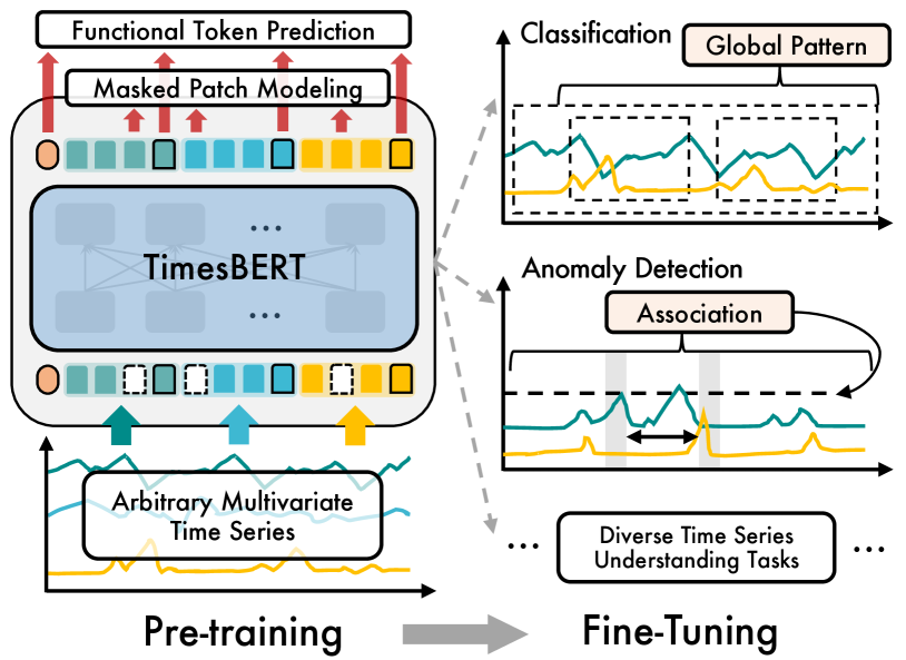
Figure 1: TimesBERT inherits and extends the pre-training and fine-tuning paradigm established by BERT, which learns generalizable representation through pre-training on large-scale datasets of arbitrary multivariate time series, and adapts the foundation model to diverse tasks of time series understanding.

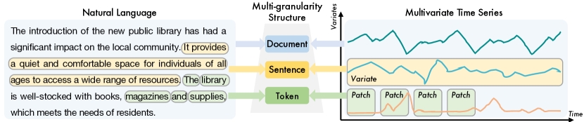
Figure 2: A multivariate time series is worth a natural language document. We propose to fully repurpose BERT for learning structured representations of time series. The representations embodying different granularities can facilitate diverse time series understanding tasks.

Foundation models (Radford et al., 2018; Dosovitskiy et al., 2020) have advanced significantly in generalization performance, making them a promising solution for data-scarce and task-agnostic applications. While prevailing GPT-style models excel in generative tasks like time series forecasting  (Das et al., 2023b; Liu et al., 2024d), they lack the ability to leverage bidirectional context, causing a critical bottleneck for global understanding. By contrast, BERT (Devlin et al., 2018) has exhibited task-versatility in natural language understanding like sentiment classification and entity identification. In addition to the primary objective of masked language modeling (MLM), BERT facilitates functional tokens [CLS] and [SEP] to enable modeling multi-granularity structures from multisentence text documents, in compliance with the auxiliary task of next-sentence prediction (NSP) to reason about sentence-wise relationships. Moreover, BERT has popularized the pre-training and fine-tuning paradigm, which can facilitate a broader range of distinct downstream tasks, which has however not been unleashed in large-scale pre-trained time series foundation models.

As illustrated in Figure 2, time series share surprising structural similarities with natural language. In addition to the prevalent practice of regarding a patch as a token (Nie et al., 2023), we observe that a sufficiently long context of time series contains rich semantics to reveal variate-wise characteristics of time series, which possesses a similar structural correspondence with a sentence in natural language. On this basis, we highlight that “a multivariate time series is worth a multisentence text document,” allowing us to inherit BERT, a general-purpose language representation learning framework with remarkable contextual awareness and multi-granularity capabilities for document-like data structures, to extract generic representations from heterogeneousness time series. The outcome pre-trained model manifested as a general feature extractor of time series, can facilitate a variety of understanding tasks. Nevertheless, while BERT adopts a fixed number of sentences with a fixed length for NSP, multivariate series can vary in both temporal length and variate number. It is required to implement a unified embedding on BERT, which is to adhere to large-scale pre-training and adaptation to various understanding tasks.

Inspired by the above motivations, we propose TimesBERT, a pre-trained foundation model for time series understanding. We conduct large-scale pre-training on 260 billion time points collected from multiple domains. We devise a unified embedding mechanism and repurpose the functional tokens in BERT to align with multivariate time series. In contrast to the previous methods that prevalently employed Channel-Independence (Nie et al., 2023), in accordance with our established framework for interpreting multivariate time series as analogous to documents, we implement the pre-training of any-variate and any-length time series to handle the discrepancies in variate- and sentence-wise modeling, which reserves inherently structured representations of time series such as variate correlation. TimesBERT achieves significant improvement on four typical understanding tasks and 113 real-world datasets compared with state-of-the-art task-specifc models, exhibiting outstanding transferability.

Our contributions can be summarized as follows:

• We rethink the common appeal of representation learning for time series understanding, and propose to treat multivariate time series as multisentence documents, revealing the advantages of BERT as a pre-trained model.

• We develop TimesBERT, which consists of a unified structured embedding and a functional token prediction task toward the multi-granularity structure of multivariate time series, fully aligning BERT to time series.

• We pre-train our model on large-scale dataset with 260 billion time points, which can be adapted with state-of-the-art results on time series classification, imputation, anomaly detection, and short-term forecasting tasks.

2 Related Works

Figure 3: Comparison between GPT (Radford et al., 2018), BERT (Devlin et al., 2018), and TimesBERT on embedding, backbone, and training objective. In contrast to BERT’s sentence pair formulation, we implement an embedding approach for data with an arbitrary number of variates and design corresponding functional tokens to accommodate the inherent irregularity of time series variates.

2.1 Time Series Understanding

Time series understanding includes a series of tasks that require structured representations and semantic extraction. Classical time series understanding methods such as Dynamic Time Warping (Berndt & Clifford, 1994) and Isolation Forests (Bandaragoda et al., 2018) make use of statistical-based representations to identify temporal motifs. Subsequent works (Wu et al., 2023; donghao & wang xue, 2024) based on CNN backbones preliminarily exhibit the ability of deep learning-based models in time series understanding. Prevailing Transformer-based models (Zhou et al., 2021b; Wu et al., 2021; Nie et al., 2023; Liu et al., 2024a) apply attention mechanisms to discover potential correlations among different granularities. However, most deep learning models are originally designed for forecasting tasks with insufficient adaptation for time series understanding.

2.2 BERT-Style Models

Developed for natural language processing, BERT (Devlin et al., 2018) conducted pioneer work in highlighting the significance of bidirectional information for data comprehension and demonstrates the effectiveness of the pre-training fine-tuning paradigm. More significantly, BERT introduces a structured and generic view to analyzing words, sentences, and documents, as opposed to simply considering natural language as entirely serialized entities.

While subsequent models extended capabilities of BERT for natural language (Liu, 2019; Lan, 2019), BERT-style models also exhibit wide-ranging effectiveness in other data modalities. MAE (He et al., 2022) employs an asymmetric encoder-decoder structure within the framework of masked modeling, achieving substantial pre-training improvements in image classification tasks. BEiT (Bao et al., 2021) employs VQVAE (Van Den Oord et al., 2017) to convert images into corresponding discrete semantic representations. Notably, models like T5 (Raffel et al., 2020) and GPT-3 (Brown et al., 2020) are the counterpart of BERT-style architecture, with encoder-decoder T5 unifying tasks into a text-to-text framework and decoder-only GPT-3 leveraging massive scale for generative modeling, pushing the limits of scalable models.

2.3 Pre-trained Time Series Models

Pre-training methods in the field of time series have achieved advancements in building task-specific and foundation models. TST (Zerveas et al., 2021) and PatchTST (Nie et al., 2023) employ BERT-style masked pre-training at the point level and patch level, respectively. SimMTM (Dong et al., 2023) attempts to integrate neighbor data comparison with masked point modeling. Free from respectively fine-tuning, TimesFM (Das et al., 2023b), Timer (Liu et al., 2024d, c), and Chronos (Ansari et al., 2024) exhibit advantages of zero-shot forecasting through large-scale pre-training. However, these models primarily focus on forecasting-based tasks, lacking task versatility for distinct understanding tasks.

There have been several initial explorations on BERT-style pre-trained models. MOMENT (Goswami et al., 2024) utilizes the T5 encoder for pre-training to achieve downstream multi-task capabilities. Moirai (Woo et al., 2024) achieves multivariate embedding and employs masked modeling by forecasting the future patches. VisionTS (Chen et al., 2024) exhibits the robust transferability of vision-masked autoencoders across different modalities. However, essential elements for structured representation learning in BERT are not fully leveraged. Therefore, we delve into aligning time series with multisentence documents and next sentence prediction tasks, thus innovatively repurposing TimesBERT’s pre-training objective to present a versatile pre-trained model for diverse understanding tasks.

3 Approach

TimesBERT employs an encoder-only Transformer to learn structured representations of multivariate time series, which is aligned with BERT (Devlin et al., 2018) in both model architecture and objective design as shown in Figure 3. By pre-training on 260 billion time points from different domains, we present a task-versatile foundation model, which can be fine-tuned for various time series understanding tasks.

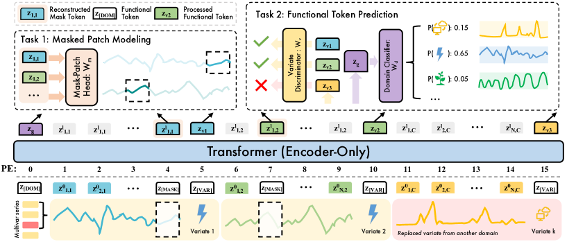
Figure 4: Illustration of the TimesBERT architecture and pre-training objectives. The input multivariate time series is embedded into a token sequence for the transformer encoder following a unified time series embedding process that includes patching, function token insertion, and flattening. Following the output from the backbone, the reconstructed patches and functional tokens are respectively fed into corresponding pre-training tasks including MPM and FTP, ultimately forming the joint optimization objective.

3.1 TimesBERT

Transformers (Vaswani et al., 2017b) are currently the de facto architecture of foundation models, especially for the vast use of GPT-style decoder-only Transformers in generative tasks. However, the primary objective of generative pre-trained models does not include learning bidirectional representations at different granularities. Thus, we adopt the BERT-style encoder-only architecture as a representation learning backbone. To cope with variable lengths in time points and variates, we design a unified time series embedding for structured representation learning.

3.1.1 Time Series Embedding

Given multivariate time series $\mathbf{X}=[\mathbf{x}_{1},\mathbf{x}_{2},...,\mathbf{x}_{C}]$ of $C$ variates, each variate $\mathbf{x}_{i}\in\mathbb{R}^{T}$ is a length-$T$ time series that will be divided into $N=\lceil\frac{T}{P}\rceil$ patches of patch length $P$:

$$\mathbf{p}_{i,c} =[\mathbf{X}_{(i-1)P+1,c},\dots,\mathbf{X}_{iP,c}],$$ (1)

$$\mathbf{z}^{0}_{i,c} =\mathbf{W}_{\texttt{in}}\mathbf{p}_{i,c}+\mathbf{PE}_{i+Pc},$$

where $\mathbf{W}_{\texttt{in}}\in\mathbb{R}^{D\times P}$ is a linear layer, and $\mathbf{PE}_{i+Pc}\in\mathbb{R}^{D}$ denotes absolute position embedding. We adopt a shared learnable embedding $\mathbf{z}_{\texttt{[MASK]}}$ in each masked position.

We repurpose the functional token [SEP], which is used for next-sentence prediction in BERT, as a learnable embedding $\mathbf{z}_{\texttt{[VAR]}}$. Inspired by the functional token [CLS] used for classifying a group of sentences in BERT, we also append a learnable embedding $\mathbf{z}_{\texttt{[DOM]}}$ at the beginning as the domain token. We formulate $\mathbf{Z}^{0}$ as the input of Transformer by stacking $(N+1)C+1$ token embeddings:

$$\mathbf{Z}^{0} =\begin{pmatrix}\mathbf{z}_{\scalebox{0.5}{{[DOM]}}}&\mathbf{z}^{0}_{1:1}&\mathbf{z}^{0}_{2:1}&...&\mathbf{z}_{\scalebox{0.5}{{[MASK]}}}&\mathbf{z}_{\scalebox{0.5}{{[VAR]}}}\\ \cdot&\mathbf{z}^{0}_{1:2}&\mathbf{z}_{\scalebox{0.5}{{[MASK]}}}&\cdots&\mathbf{z}^{0}_{N,2}&\mathbf{z}_{\scalebox{0.5}{{[VAR]}}}\\ \cdot&\vdots&\vdots&\ddots&\vdots&\vdots\\ \cdot&\mathbf{z}^{0}_{1:C}&\mathbf{z}^{0}_{2:C}&\cdots&\mathbf{z}^{0}_{N,C}&\mathbf{z}_{\scalebox{0.5}{{[VAR]}}}\end{pmatrix}.$$ (2)

We implement packing (Raffel et al., 2020) to simultaneously train on different multivariate time series in one large context length (512 tokens in TimesBERT). In addition to aggregating global information, the functional token helps separate different training samples.

We adopt an encoder-only Transformer with dimensions $D$ and $L$ layers as the backbone of TimesBERT, which forwards the flattened token embeddings:

$$\mathbf{Z}^{l}=\operatorname{TrmBlock}(\mathbf{Z}^{l-1}),\ l=1,\dots,L.$$ (3)

As shown in Figure 4, we extend the 1D format of word sequences in BERT to accommodate multivariate time series with arbitrary variates and time points. In conjunction with the pre-training tasks designed, patterns at the patch level, variate level, and sample level are aggregated on the corresponding functional tokens, which ultimately forms multi-granularity representation extraction.

3.2 Pre-training TimesBERT

We design two pre-training objectives for structured time series to acquire a generic understanding.

3.2.1 Task #1: Masked Patch Modeling

Inspired by the masked language modeling task utilized in BERT, we employ masked patch modeling (MPM) to provide a pedestal understanding ability for the foundation model. Given the input token sequence, we adopt a masked ratio $\alpha=25\%$ for non-functional tokens. To minimize the discrepancy between pre-training and fine-tuning tasks, these selected masked tokens are then actually replaced by $\mathbf{z}_{\texttt{[MASK]}}$ with a $90\%$ probability. Here let $\mathbf{z}_{i}$ denote reconstructed token at position $i$, let $S=\alpha NC$ denote the total number of masked patches, and we denote reconstructed patches as $\{\widehat{\mathbf{p}}_{i}\}_{i=1}^{S}$. We use a linear layer $\mathbf{W}_{\texttt{out}}\in\mathbb{R}^{D\times P}$ to project tokens to reconstructed patches:

$$\{\widehat{\mathbf{p}}_{i}\}_{i=1}^{S}=\{\mathbf{z}_{i}\}_{i=1}^{S}\mathbf{W}_{\texttt{out}}.$$ (4)

Given the ground truth of masked patches as $\{\mathbf{p}_{i}\}_{i=1}^{S}$, the masked patch modeling objective is formulated as:

$$\mathcal{L}_{\text{MPM}}=\frac{1}{SP}\sum\limits_{i=1}^{S}||\mathbf{p}_{i}-\widehat{\mathbf{p}}_{i}||_{2}^{2}.$$ (5)

Equation 5 enhances the basic model capability to extract temporal representations from local variations. Nevertheless, ablation studies 4.5 indicate that MPM alone is insufficient to provide optimal transfer ability toward downstream tasks. For tasks requiring explicit understanding of global representations, such as classification and anomaly detection, it is necessary to propose a pre-training task that better aligns with the document-like structure of time series data.

3.2.2 Task #2: Functional Token Prediction

Despite the goal of masked patch modeling to model temporal patterns in a single time series, it struggles to explicitly handle inter-variate relationships and effectively aggregate the overall characteristics of variates. Inspired by next sentence prediction (NSP) task in BERT, we propose Functional Token Prediction (FTP) relying on special tokens.

We design a variate discrimination task. Given a multivariate time series with $C\geq 2$, we randomly replace one variate with another from another dataset. The task of the model is to identify the replaced variate by its own variation patterns. Here let $\mathbf{z}_{\mathbf{v}_{c}}$ denote the output of $\mathbf{z}_{\texttt{[VAR]}}$ of $n$-th variate, and we project $\mathbf{z}_{\mathbf{v}_{c}}$ with a linear layer $\mathbf{W}_{\texttt{VAR}}\in\mathbb{R}^{D\times 2}$ to classify whether a variate originated the same as other variates.

Here let $\mathbf{z}_{g}$ denote the output of $\mathbf{z}_{\texttt{[DOM]}}$. Based on the domain token $\mathbf{z}_{g}$, we propose a domain classification task. With $M$ datasets indexed in pre-training, the backbone provides outputs, and $\mathbf{z}_{g}$ is fed into a linear layer $\mathbf{W}_{\texttt{DOM}}\in\mathbb{R}^{D\times M}$ to predict the dataset index of the series.

Based on the aforementioned process, the functional token prediction objective can be formulated as follows:

$$\mathcal{L}_{\scalebox{0.5}{\text{FTP}}}=-\sum_{c=1}^{C}\sum_{i=1}^{2}\mathbf{y}^{c}_{i}\log(\mathbf{z}_{\mathbf{v}_{c}}\mathbf{W}_{\scalebox{0.3}{{VAR}}})_{i}-\sum_{i=1}^{M}\mathbf{y}^{d}_{i}\log(\mathbf{z}_{g}\mathbf{W}_{\scalebox{0.3}{{DOM}}})_{i},$$ (6)

where the one-hot vector $\mathbf{y}^{c}$ denotes labels marking whether $\mathbf{v}_{c}$ is the replaced variate, and the one-hot vector $\mathbf{y}^{d}$ denotes the index of the dataset.

Finally, the training objective is represented as follows:

$$\mathcal{L}=\mathcal{L}_{\text{MPM}}+\mathcal{L}_{\text{FTP}}.$$ (7)

Our functional token prediction task treats each variate as a time series sentence, requiring them to distribute and aggregate with one another to identify their similarities and differences in relation to the entire sequence. As functional tokens learn representations at varying granularities, they enhance task versatility during downstream adaptation, allowing a series of token embeddings to be employed for understanding time series patches, variables, and domains. Following the pre-training phase, the task head is removed, while the Transformer backbone is adapted for representation extraction during fine-tuning. This process effectively decouples the pre-trained backbone from the task design.

3.3 Pre-Training Data

We construct large-scale time series corpora from various sources. We adopt the LOTSA dataset (Woo et al., 2024) as the main body of the pre-training dataset, taking into account the needs of the basic model for multi-domain and pattern diversity requirements. Simultaneously, there is a notable discrepancy in data features between understanding-oriented domains, such as medical (Gow et al., 2023), and pre-training data used for forecasting, thus to account for the varying temporal dynamics and variate correlations of time series across different tasks, we incorporate the UEA Archive (Bagnall et al., 2018) to achieve a balanced data portrait, forming a large-scale corpus with a total of 260 billion time points. Based on our structure-preserving design for multivariate time series, TimesBERT fully leverages time series native during large-scale pre-training to achieve rapid and effective transfer for complex time series tasks.

3.4 Fine-Tuning TimesBERT

Analogous to the fine-tuning methodology employed with BERT, we adopt a trainable output layer during the fine-tuning phase of TimesBERT to accommodate various downstream datasets. Considering the low er information density, we utilize all tokens to ensure a comprehensive representation when migrating to the classification, while tokens at the corresponding positions are directly used as representations for imputation and anomaly detection. For diverse understanding tasks, the fine-tuning paradigm of BERT-style models empirically exhibits advantages compared to the prevailing zero-shot paradigm of GPT-style models.

4 Experiments

In order to validate the capacity of TimesBERT for typical understanding scenarios, we conduct experiments in time series classification, imputation, short-term forecasting, and anomaly detection tasks. We compare TimesBERT with state-of-the-art task-specific and general models and exhibit the benefit of pre-training. In addition, we conducted comprehensive ablation studies to evaluate various aspects of the model design and its capabilities. We provide implementation details and model configurations in Appendix A.

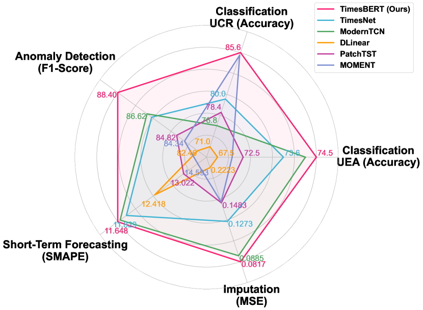
Figure 5: Overall Performance of TimesBERT.

4.1 Classification

Setups

Time series classification represents a typical data understanding task. During the feature extraction process of the pre-trained model, capturing temporal patterns necessitates that the classifier possesses robust global comprehension capabilities. We utilize two benchmark datasets for time series classification. Specifically, we employ 10 subsets from the UEA Archive (Bagnall et al., 2018) and 91 subsets from the UCR Archive (Dau et al., 2019), spanning diverse domains such as biology, physics, environmental monitoring, human activity recognition, and finance, among others. These datasets encompass varying variate numbers and sequence lengths which exhibit diversity in granularity.

Figure 6: Averaged results of classification task on UEA and UCR Archive. We illustrate an extensive range of analytical baselines, among which TimesBERT achieved state-of-the-art performance in two classification benchmarks. The results of previous methods are directly taken down from previous literature for fair comparison. See Table 5 and Table 6 for full results.

Results

Figure 6 illustrates the inference outcomes of our model on UEA and UCR Archive. Compared to statistical methods, state-of-the-art deep learning models, and classical unsupervised representation learning methods, the average classification accuracy of TimesBERT shows consistent performance enhancements. Notably, given the substantial variations in sequence length, number of variates, change patterns, and class counts across existing time series classification benchmarks, TimesBERT exhibits comprehensive improvements across over one hundred benchmark datasets.

4.2 Anomaly Detection

Setups

Time series anomaly detection is a widely discussed task aimed at discerning anomalous data segments, which is of great importance in actual time series analysis. We include five widely-used anomaly detection benchmarks into our experiments, namely: SMD (Su et al., 2019), MSL (Hundman et al., 2018), SMAP (Hundman et al., 2018), SWaT (Mathur & Tippenhauer, 2016), PSM (Abdulaal et al., 2021). Our evaluation follows the unsupervised time series anomaly detection logic mentioned in previous works such as TimesNet (Wu et al., 2023), where datasets are split into non-overlapping sliding windows, and the reconstruction error is applied as the anomaly criterion.

Results

Our experiments result in table 1 shows that TimesBERT performs better than previous sota baselines such as TimesNet (Wu et al., 2023). We highlight that TimesBERT’s improvements are consistent across all time series anomaly detection benchmarks, which demonstrates the robust adaptability of pre-trained models to complex downstream understanding tasks and diverse datasets.

Table 1: Anomaly detection results. We calculate the F1-score (as %) for each dataset. *. means the *former. A higher value of the F1-score indicates a better performance. See Table 12 for full results.

Model	TimesBERT	MTCN	TimesNet	ETS.	FED.	LightTS	DLinear	NS.	Auto.	Pyra.	Anomaly.	Informer	Reformer	LogTrans	Trans.
	(Ours)	(2024)	(2023)	(2022)	(2022)	(2022)	(2023a)	(2022)	(2021)	(2021)	(2021)	(2021a)	(2020)	(2019)	(2017a)
SMD	86.04	85.81	85.81	83.13	85.08	82.53	77.10	84.72	85.11	83.04	85.49	81.65	75.32	76.21	79.56
MSL	88.07	84.92	85.15	85.03	78.57	78.95	84.88	77.50	79.05	84.86	83.31	84.06	84.40	79.57	78.68
SMAP	75.69	71.26	71.52	69.50	70.76	69.21	69.26	71.09	71.12	71.09	71.18	69.92	70.40	69.97	69.70
SWaT	93.95	93.86	91.74	84.91	93.19	93.33	87.52	79.88	92.74	91.78	83.10	81.43	82.80	80.52	80.37
PSM	98.27	97.23	97.47	91.76	97.23	97.15	93.55	97.29	93.29	82.08	79.40	77.10	73.61	76.74	76.07
Avg. F1	88.40	86.62	86.34	82.87	84.97	84.23	82.46	82.08	84.26	82.57	80.50	78.83	77.31	76.60	76.88

4.3 Imputation

Setups

Given the pervasive occurrence of missing values in real-world industrial production scenarios, we evaluate the effectiveness of time series imputation tasks, where bidirectional information is significantly important for enhancing the model’s ability to analyze missing segments. Additionally, this task necessitates that the model comprehends and encapsulates the overall features of the series through high-order representations, revealing the advantages of TimesBERT. Since value missing in real scenarios often occurs in continuous segments, we employ patch-level imputation for evaluation following Timer (Liu et al., 2024d), which is more challenging than point-level imputation.

Figure 7: Averaged results of imputation tasks. We randomly mask $\{12.5\%,25\%,37.5\%,50\%\}$ patches. The results are averaged from 4 mask ratios. See Table 7 and Table 10 for full results.

Results

We conduct comprehensive evaluations on selected six classical benchmarks with four different mask ratios in order to avoid data leakage caused by pre-trained corpus and compared them with advanced general and foundation models. As shown in Table 7, TimesBERT achieves a $7.7\%$ loss reduction compared to the state-of-the-art model on this task. In addition, we test the benefits of model pre-training under the data scarcities of $\{5\%,20\%,100\%\}$. As shown in Figure 8, the pre-trained model gives a significant improvement with fewer fine-tuning samples.

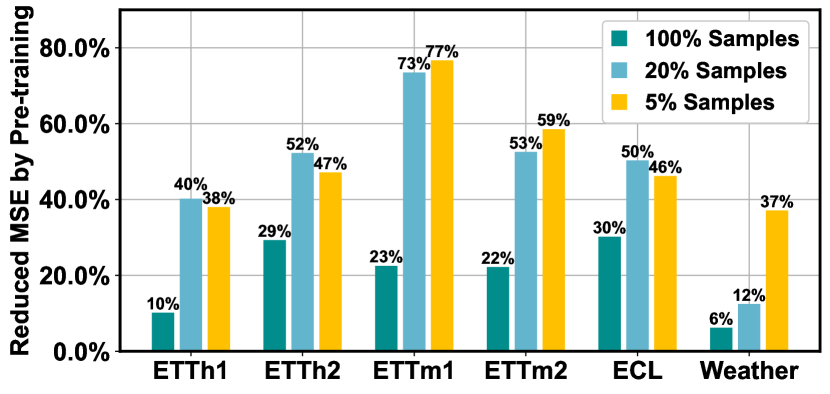
Figure 8: Pre-training benefit of TimesBERT on the downstream imputation task with $100\%$, $20\%$ and $5\%$ available samples. Each dataset is imputed with four mask ratios and we calculate the average reduced imputation error in MSE relative to training from scratch. See Table 7, Table 8 and Table 9 for full results.

4.4 Short-Term Forecasting

Setups

Short-term time series forecasting is extensively utilized in domains such as meteorological prediction, market analysis, and finance. Unlike long-term forecasting tasks, which depend on capturing consistent local change patterns within the retrospective window and require robust model roll-out capabilities, short-term forecasting emphasizes providing trend predictions for the forecast horizon based on the overall characteristics of the series. Consequently, it is more suitable for models with understanding capabilities. For this task, we employ the M4 dataset (Spyros Makridakis, 2018) as a benchmark. We adhere to the evaluation established by TimesNet (Wu et al., 2023).

Table 2: Average short-term forecasting results on the M4 (Spyros Makridakis, 2018). Full results are provided in Table 11.

Method		TimesBERT	MTCN	TimesNet	iTrans.	Koopa	NHiTS	DLinear	PatchTST	MICN	TiDE	MOMENT	NBEATS
		(Ours)	(2023)	(2024)	(2024a)	(2023)	(2023)	(2023b)	(2023)	(2022)	(2023a)	(2024)	(2019)
Average	SMAPE	11.648	11.698	11.829	12.684	11.863	11.960	12.418	13.022	13.023	13.950	14.593	11.910
	MASE	1.560	1.556	1.585	1.764	1.595	1.606	1.656	1.814	1.836	1.940	2.161	1.613
	OWA	0.837	0.838	0.851	0.929	0.858	0.861	0.891	0.954	0.960	1.020	1.103	0.862

Results

We evaluate well-acknowledged forecasting models, including iTransformer (Liu et al., 2024a), PatchTST (Nie et al., 2023) and TimesNet (Wu et al., 2023), by three widely accepted metrics on the M4 dataset. As shown in Table 2, TimesBERT outperforms previous models consistently on all average SMAPE and OWA.

4.5 Model Analysis

Pre-training Tasks

During the pre-training phase, we employ two distinct pre-training tasks and concurrently optimize three task-specific heads, among which there is explicit complementary relation. We conduct an ablation study on the tasks and compare in detail the performance of pre-trained TimesBERT with and without the functional token prediction task before transferring to time series classification tasks. On this basis, we examine the impact of functional token selection during the fine-tuning stage.

As shown in Table 3, on average, all our pre-training tasks and functional tokens while fine-tuning yield positive improvements. Notably, the inclusion of functional tokens provides a significant boost to classification performance, confirming their ability to aggregate relevant representation.

Table 3: Ablation of pre-training tasks. D in the “pre-train” row means using domain classification, and V means using variate discrimination; In the “fine-tuning” row, D means $\mathbf{z}_{\texttt{[DOM]}}$ is used for the task head while fine-tuning, and V means $\mathbf{z}_{\texttt{[VAR]}}$ is used.

Pre-train	D+V			D	None
Fine-tune	D+V	D	None	D	None
EC	34.60	34.22	33.46	30.04	32.32
FD	68.67	68.67	69.44	68.93	69.55
HW	36.59	36.59	36.12	35.76	35.18
HB	78.54	78.54	77.56	78.05	78.54
JV	97.57	97.57	98.38	98.38	98.38
SRS1	93.17	93.17	93.52	91.47	90.78
SRS2	58.33	58.33	57.22	59.44	57.22
SWJ	99.41	99.41	99.50	99.27	99.32
SW	95.00	95.00	95.31	94.38	93.44
Avg.	73.54	73.50	73.39	72.86	72.75

Initialization

Recent studies on large language models and vision models for time series (Zhou et al., 2023; Liu et al., 2024b; Chen et al., 2024) have demonstrated the advantages of leveraging pre-trained models on other modalities for time series modeling to some extent, while we posit that time series exhibit more complex intrinsic variation patterns. Therefore, in this ablation study, we attempt to directly initialize TimesBERT using a pre-trained BERT model and compare its performance with that of a normal pre-trained TimesBERT on classification tasks.

Figure 9 illustrates the inclusion of different initialization methods alongside a random initialization as a control group, which highlights the fundamental difference among linguistic manifolds, image semantic space, and time series, while also demonstrating the significant improvements achieved by our pre-trained models. These findings underscore the importance of native time-series pre-training.

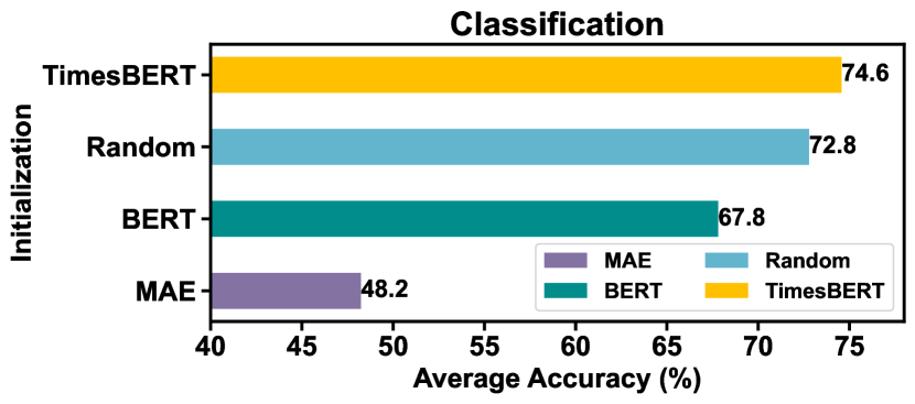
Figure 9: We initialize TimesBERT for downstream tasks using three methods: (1) pre-trained TimesBERT model, (2) random initialization, (3) A Vision Transformer (Dosovitskiy et al., 2020) pre-trained with Masked Autoencoder  (He et al., 2022), and (4) a BERT (Devlin et al., 2018) model pre-trained on language.

Multivariate Modeling

Time series understanding tasks typically require robust multivariate modeling capabilities, in which capturing multivariate correlations is often essential for accurately representing the overall data features. Nevertheless, existing foundation model designs often employ Channel Independence (CI) to avoid interference from variate modeling (Liu et al., 2024d; Ansari et al., 2024). We conduct ablation studies on classification and imputation tasks utilizing datasets with explicit multivariate features.

Figure 10 indicates that in both tasks, compared to employing CI to mitigate the interference from variate relationships, TimesBERT consistently leverages the variate correlations to achieve benefits while supporting multivariate inputs.

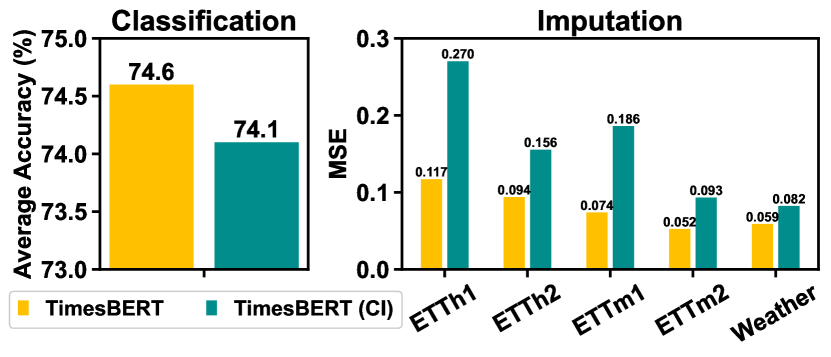
Figure 10: Ablation of TimesBERT’s multivariate capabilities on classification and imputation tasks. CI indicates that the model uses the Channel Independence strategy (Nie et al., 2023).

5 Conclusion and Future Work

In this paper, we highlight that multivariate time series and multisentence text documents exhibit a similar multi-granularity structure. Inspired by BERT which facilitates structured representation learning for agnostic downstream tasks, we leverage BERT-style architectures for generic time series understanding, which is achieved by repurposing masked modeling and functional token prediction for arbitrary multivariate time series. By large-scale pre-training on 260 billion time points across different domains, TimesBERT surpasses state-of-the-art models across four typical understanding tasks, which validates the exceptional generalization capabilities that BERT can also offer in the realm of time series analysis. We will explore the adaption of functional tokens and delve into domain-universal pre-training for more time series understanding tasks.

Appendix A Implementation Details

A.1 Pre-training

All experiments in this paper are implemented in PyTorch (Paszke et al., 2019) and conducted on NVIDIA 4090 GPU. We used AdamW as the optimizer in the pre-training phase with $\beta_{1}=0.9,\beta_{2}=0.99$, and applied the cosine annealing algorithm for learning rate decay. Specifically, we use $1\times 10^{-4}$ as the initial learning rate and $2\times 10^{-7}$ as the final learning rate. To conduct fair ablation experiments, all our pre-trained models are trained for $30000$ steps on a large-scale time series corpus, where the batch size is $40\times 8=320$ and the context length of each sequence, that is, the number of patches, is $512$. To improve the convergence speed, we use the packing (Raffel et al., 2020) for large-scale pre-training.

For alignment with BERT (Devlin et al., 2018), our pre-trained model size is the same as $\mathbf{BERT}_{\mathbf{base}}$, i.e., we denote the number of layers as $L$, the hidden size as $H$, and the number of self-attention heads as $A$, then the model size is $L=12,H=768,A=12$, and the total number of parameters is $85.6$M. Considering the diversity of downstream datasets, we use models with different patch lengths on different tasks to adapt to diverse understanding tasks, including $36$ for classification, $24$ for imputation, and $4$ for short-term forecasting and anomaly detection tasks.

A.2 Downstream Tasks

Table 4: Dataset descriptions. The dataset size is organized in (Train, Validation, Test). * means that different subsets have different values

Tasks	Dataset	Variate	Series Length	Dataset Size	Information (Frequency)
	M4-Yearly	1	6	(23000, 0, 23000)	Demographic
	M4-Quarterly	1	8	(24000, 0, 24000)	Finance
Forecasting	M4-Monthly	1	18	(48000, 0, 48000)	Industry
(short-term)	M4-Weakly	1	13	(359, 0, 359)	Macro
	M4-Daily	1	14	(4227, 0, 4227)	Micro
	M4-Hourly	1	48	(414, 0, 414)	Other
Imputation	ETTm1, ETTm2	7	192	(34465, 11521, 11521)	Electricity (15 mins)
	ETTh1, ETTh2	7	192	(8545, 2881, 2881)	Electricity (15 mins)
	Electricity	321	192	(18317, 2633, 5261)	Electricity (15 mins)
	Weather	21	192	(36792, 5271, 10540)	Weather (10 mins)
	EthanolConcentration	3	1751	(261, 0, 263)	Alcohol Industry
	FaceDetection	144	62	(5890, 0, 3524)	Face (250Hz)
	Handwriting	3	152	(150, 0, 850)	Handwriting
	Heartbeat	61	405	(204, 0, 205)	Heart Beat
Classification	JapaneseVowels	12	29	(270, 0, 370)	Voice
	PEMS-SF	963	144	(267, 0, 173)	Transportation (Daily)
	SelfRegulationSCP1	6	896	(268, 0, 293)	Health (256Hz)
	SelfRegulationSCP2	7	1152	(200, 0, 180)	Health (256Hz)
	SpokenArabicDigits	13	93	(6599, 0, 2199)	Voice (11025Hz)
	UWaveGestureLibrary	3	315	(120, 0, 320)	Gesture
	UCR Archive	1	*	(*, 0, *)	*
	SMD	38	40	(566724, 141681, 708420)	Server Machine
Anomaly	MSL	55	40	(44653, 11664, 73729)	Spacecraft
Detection	SMAP	25	40	(108146, 27037, 427617)	Spacecraft
	SWaT	51	40	(396000, 99000, 449919)	Infrastructure
	PSM	25	40	(105984, 26497, 87841)	Server Machine

A.2.1 Classification

The time series classification task is a typical understanding task, which requires the model to make a holistic judgment based on the global representation. It is worth mentioning that, different from the multivariate time series prediction task that has been discussed more, part of the variate information and variate correlation in the classification of time series samples may be indispensable for accurate classification, so the multivariate modeling ability of the model is tested. In this experiment, we choose the multivariate data set UEA Archive (Bagnall et al., 2018) and the univariate UCR dataset (Dau et al., 2019) together as the benchmark data set. For a fair comparison, we keep our evaluation aligned with Time-Series-Library (Wang et al., 2024). See Table 4 for detailed information on the dataset.

A.2.2 Anomaly Detection

Multivariate time series anomaly detection tasks normally inherit the characteristics of having various anomalous segment lengths. Some anomalous segments are within 10 data points while others may be up to hundreds of data points. To study a representation that is capable of detecting subtle anomalies, we shrink the patch length to 4 during the large scale pertaining. Correspondingly, we also reduce the hidden dimension to 256 and the attention layers to 4 to avoid over-fitting. During downstream fine-tuning, we adopt a different input length of 40 compared to previous works such as TimesNet (Wu et al., 2023), corresponding to 10 input tokens. For a fair comparison, we keep our evaluation process aligned with previous works implemented in the Time Series Library. See Table 4 for detailed details of the dataset.

A.2.3 Imputation

The multivariate time series imputation task we employ requires the model to impute against continuous missing values that occur frequently in real scenarios. At the same time, our test uses the multivariate benchmark data set to test the ability of the model to use the mutual hint between variates for collaborative imputation. Our benchmark datasets include (1) ETT (Zhou et al., 2021b) containing 7 variates of power transformers, (2) ECL (Wu et al., 2021) consisting of hourly electricity consumption data from 321 customers (3) Weather (Wu et al., 2021) consisting of 21 meteorological variates. For a fair comparison, we keep our evaluation process aligned with previous works implemented in Timer (Liu et al., 2024d). See Table 4 for details of the dataset.

A.2.4 Short-term Forecasting

Compared with the long-term forecasting of time series, the short-term forecasting of time series has a higher ability demand for the model to capture the global trend and overall pattern of the data in the lookback window, which adapts to the multi-granularity structure capture ability of TimesBERT. The experiment is carried out on the M4 (Spyros Makridakis, 2018), which includes six univariate sequences with different change frequencies from various real scenes and can effectively prove the ability of the model to perform on data with different change patterns. For a fair comparison, we keep our evaluation aligned with previous works implemented in the Time-Series-Library. See Table 4 for details of the dataset.

Appendix B Representation Analysis

To verify the effectiveness of TimesBERT representation, we perform 2D t-SNE (Van der Maaten & Hinton, 2008) representation visualization on many classification datasets in a zero-shot setting. In Figure 11, we present the example visualization of “SpokenArabicDigits”, “UWaveGestureLibrary”, and “JapeneseVowels” from the UEA archive as well as “ElectricDevices”, “Crop”, “ECG5000”, “Wafer”, “ChlorineConcentration”, and “FacesUCR” from the UCR archive. Small clusters of the same color in visualization suggest that samples from a specific class tend to have more similar high-dimensional representations. Such results show that TimesBERT is capable of acquiring distinct representations of different classes after systematic pertaining without data-specific fine-tuning.

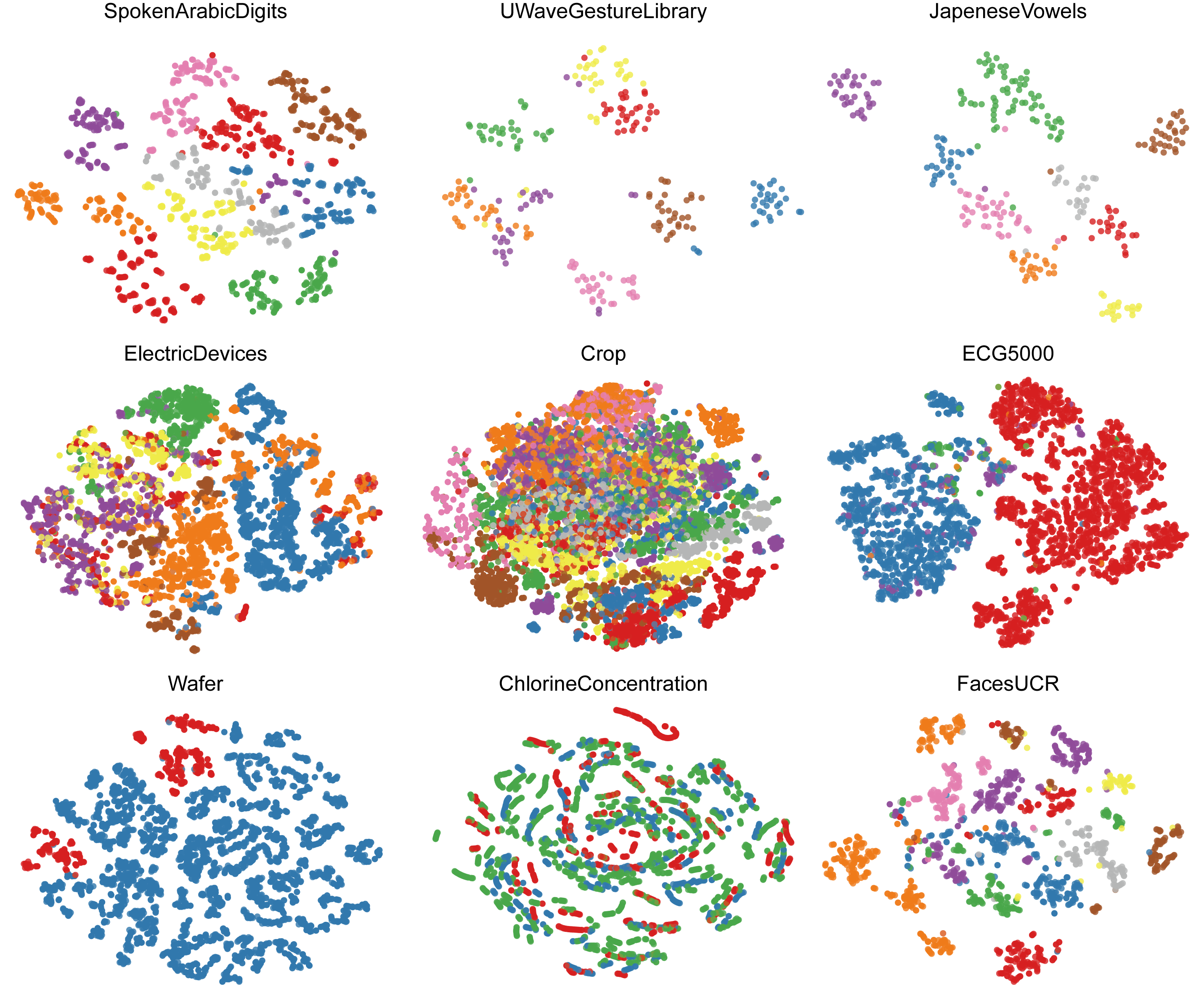
Figure 11: The t-SNE representation visualization of pre-trained TimesBERT on examples from the UEA and UCR classification datasets. Each color in visualization stands for a specific target class in an example dataset.

Appendix C Full Results

Due to the limitation of space in the main text, we present detailed results of all time series understanding tasks in this section, including time series classification, imputation, short-term forecasting, and anomaly detection.

Time series classification results are as follows: full results of UEA classification in Table 5 and full results of UCR classification in Table 6. Time series imputation results are as follows: imputation with 100% samples in Table 7, imputation with 20% samples in Table 8, imputation with 5% samples in Table 9, and full results of imputation in Table 10. Full results of short-term forecasting in Table 11. Full results of anomaly detection in Table 12.

Table 5: Full results for the classification task on UEA Archive. $\ast.$ in the Transformers indicates the name of $\ast$former. We report the classification accuracy (%) as the result. The standard deviation is within 0.1%.

Datasets / Models	Classical methods			RNN			TCN	Transformers									MLP		CNN		Pre-trained
	DTW	XGBoost	Rocket	LSTM	LSTNet	LSSL	TCN	Trans.	Re.	In.	Pyra.	Auto.	Station.	FED.	ETS.	Flow.	DLinear	LightTS.	TimesNet	MTCN	MOMENT	TimesBERT
	(1994)	(2016)	(2020)	(1997)	(2018)	(2022)	(2019)	(2017a)	(2020)	(2021a)	(2021)	(2021)	(2022)	(2022)	(2022)	(2022)	(2023a)	(2022)	(2023)	(2024)	(2024)	(Ours)
EthanolConcentration	32.3	43.7	45.2	32.3	39.9	31.1	28.9	32.7	31.9	31.6	30.8	31.6	32.7	31.2	28.1	33.8	32.6	29.7	35.7	36.3	30.0	34.6
FaceDetection	52.9	63.3	64.7	57.7	65.7	66.7	52.8	67.3	68.6	67.0	65.7	68.4	68.0	66.0	66.3	67.6	68.0	67.5	68.6	70.8	68.9	68.6
Handwriting	28.6	15.8	58.8	15.2	25.8	24.6	53.3	32.0	27.4	32.8	29.4	36.7	31.6	28.0	32.5	33.8	27.0	26.1	32.1	30.6	35.1	36.5
Heartbeat	71.7	73.2	75.6	72.2	77.1	72.7	75.6	76.1	77.1	80.5	75.6	74.6	73.7	73.7	71.2	77.6	75.1	75.1	78.0	77.2	73.7	78.5
JapaneseVowels	94.9	86.5	96.2	79.7	98.1	98.4	98.9	98.7	97.8	98.9	98.4	96.2	99.2	98.4	95.9	98.9	96.2	96.2	98.4	98.8	95.7	97.5
PEMS-SF	71.1	98.3	75.1	39.9	86.7	86.1	68.8	82.1	82.7	81.5	83.2	82.7	87.3	80.9	86.0	83.8	75.1	88.4	89.6	89.1	85.5	83.8
SelfRegulationSCP1	77.7	84.6	90.8	68.9	84.0	90.8	84.6	92.2	90.4	90.1	88.1	84.0	89.4	88.7	89.6	92.5	87.3	89.8	91.8	93.4	88.7	93.1
SelfRegulationSCP2	53.9	48.9	53.3	46.6	52.8	52.2	55.6	53.9	56.7	53.3	53.3	50.6	57.2	54.4	55.0	56.1	50.5	51.1	57.2	60.3	55.0	58.3
SpokenArabicDigits	96.3	69.6	71.2	31.9	100.0	100.0	95.6	98.4	97.0	100.0	99.6	100.0	100.0	100.0	100.0	98.8	81.4	100.0	99.0	98.7	99.4	99.4
UWaveGestureLibrary	90.3	75.9	94.4	41.2	87.8	85.9	88.4	85.6	85.6	85.6	83.4	85.9	87.5	85.3	85.0	86.6	82.1	80.3	85.3	86.7	90.0	95.0
Average Accuracy	67.0	66.0	72.5	48.6	71.8	70.9	70.3	71.9	71.5	72.1	70.8	71.1	72.7	70.7	71.0	73.0	67.5	70.4	73.6	74.2	72.2	74.5

Table 6: Full results of the classification task on UCR Archive (Dau et al., 2019).

Datasets	DTW	TS2Vec	T-Loss	TNC	TS-TCC	TST	CNN	Encoder	FCN	MCDNN	ResNet	TimesNet	MTCN	t-LeNet	TWIESN	MLP	DLinear	PatchTST	MOMENT	GPT4TS	TimesBERT
AllGestureWiimoteX	71.6	77.7	76.3	69.7	69.7	25.9	41.1	47.5	71.3	26.1	74.1	52.7	49.1	10.0	52.2	47.7	31.7	55.6	71.7	23.7	64.7
AllGestureWiimoteY	72.9	79.3	72.6	74.1	74.1	42.3	47.9	50.9	78.4	42.0	79.4	56.3	50.1	10.0	60.0	57.1	34.1	62.3	76.7	16.0	72.1
AllGestureWiimoteZ	64.3	74.6	72.3	68.9	68.9	44.7	37.5	39.6	69.2	28.7	72.6	51.1	48.0	10.0	51.6	43.9	33.9	52.7	72.0	11.6	64.0
ArrowHead	70.3	85.7	76.6	73.7	73.7	77.1	71.7	63.0	84.3	67.8	83.8	78.9	76.6	30.3	68.9	78.4	66.9	66.3	86.9	42.9	89.1
BME	90.0	99.3	99.3	93.3	93.3	76.0	94.7	82.7	83.6	89.6	99.9	80.0	66.7	33.3	81.9	90.5	70.0	90.0	90.0	36.7	100.0
Beef	63.3	76.7	66.7	60.0	60.0	50.0	76.7	70.7	68.0	50.7	75.3	95.0	90.0	20.0	52.7	71.3	90.0	73.3	90.0	16.7	80.0
BeetleFly	70.0	90.0	80.0	80.0	80.0	100.0	90.0	62.0	91.0	63.0	85.0	70.0	70.0	50.0	79.0	88.0	80.0	75.0	75.0	70.0	95.0
BirdChicken	75.0	80.0	85.0	65.0	65.0	65.0	71.0	51.0	94.0	54.0	88.0	93.3	80.0	50.0	62.0	74.0	90.0	80.0	99.3	55.0	90.0
CBF	99.7	100.0	98.3	99.8	99.8	89.8	95.9	97.7	99.4	90.8	99.6	96.1	83.4	33.2	89.6	86.9	77.8	96.3	97.9	83.0	95.9
Chinatown	95.7	96.5	95.1	98.3	98.3	93.6	97.7	96.6	98.0	94.5	97.8	98.3	96.5	72.6	82.5	87.2	83.1	98.3	98.5	85.7	98.0
ChlorineConcentration	64.8	83.2	74.9	75.3	75.3	56.2	60.8	58.3	81.7	66.2	85.3	69.2	62.6	53.3	55.4	80.0	58.8	62.2	73.9	56.5	66.3
Coffee	100.0	100.0	100.0	100.0	100.0	82.1	100.0	88.6	100.0	97.9	100.0	92.9	100.0	50.7	97.9	99.3	100.0	100.0	100.0	67.9	100.0
CricketX	75.4	78.2	71.3	73.1	73.1	38.5	53.5	64.4	79.4	51.3	79.9	58.5	54.4	7.4	62.7	59.1	32.1	64.6	77.4	53.1	74.6
CricketY	74.4	74.9	72.8	71.8	71.8	46.7	58.2	63.9	79.3	52.1	81.0	58.7	57.4	8.5	65.2	59.8	39.0	67.9	81.5	52.1	74.9
CricketZ	75.4	79.2	70.8	71.3	71.3	40.3	50.1	65.1	81.0	48.4	80.9	57.2	56.7	6.2	64.3	62.9	31.8	68.7	77.9	39.7	72.8
Crop	66.5	75.6	72.2	74.2	74.2	71.0	67.0	76.0	73.8	68.7	74.3	77.5	76.4	4.2	48.9	61.8	68.1	72.5	74.8	34.1	76.2
DiatomSizeReduction	96.7	98.4	98.4	97.7	97.7	96.1	95.4	88.0	34.6	64.6	30.1	95.8	87.9	30.1	91.4	90.9	88.9	88.6	96.7	98.7	98.4
DistalPhalanxOutlineAgeGroup	77.0	72.7	72.7	75.5	75.5	74.1	75.8	76.1	71.8	72.9	71.8	78.4	79.9	43.3	70.5	64.7	66.9	75.5	79.1	48.9	80.6
DistalPhalanxOutlineCorrect	71.7	76.1	77.5	75.4	75.4	72.8	77.2	72.4	76.0	75.9	77.0	77.5	78.6	58.3	71.1	72.7	69.9	75.7	76.4	65.9	78.6
DistalPhalanxTW	59.0	69.8	67.6	67.6	67.6	56.8	67.1	69.4	69.5	68.5	66.3	72.7	73.4	28.5	59.1	61.0	69.8	73.4	70.5	61.9	71.2
DodgerLoopDay	50.0	56.2	NaN	NaN	NaN	20.0	31.2	48.7	14.3	30.5	15.0	56.3	57.5	16.0	59.3	16.0	57.5	51.3	58.8	20.0	57.5
DodgerLoopGame	87.7	84.1	NaN	NaN	NaN	69.6	81.6	81.0	76.8	87.7	71.0	87.0	81.9	47.8	71.6	86.5	79.0	83.3	88.4	71.7	86.2
DodgerLoopWeekend	94.9	96.4	NaN	NaN	NaN	73.2	97.4	98.3	90.4	97.8	95.2	98.6	97.8	73.9	95.4	97.8	97.1	98.6	98.6	80.4	98.6
ECG200	77.0	92.0	94.0	88.0	88.0	83.0	81.6	88.4	88.8	83.8	87.4	74.8	74.8	64.0	87.4	91.4	64.7	91.0	75.5	79.0	93.0
ECG5000	92.4	93.5	93.3	94.1	94.1	92.8	92.8	94.1	94.0	93.3	93.5	89.0	86.0	58.4	92.2	93.0	83.0	94.1	94.0	58.4	95.2
ECGFiveDays	76.8	100.0	100.0	87.8	87.8	76.3	87.4	84.2	98.5	80.0	96.6	94.0	94.3	49.7	72.3	97.3	94.0	95.8	94.8	56.1	99.9
Earthquakes	71.9	74.8	74.8	74.8	74.8	74.8	70.9	74.0	72.5	74.8	71.2	90.0	88.2	74.8	74.8	72.7	94.3	74.8	100.0	74.8	79.1
ElectricDevices	60.2	72.1	70.7	68.6	68.6	67.6	68.6	70.2	70.6	65.3	72.8	70.9	63.8	24.2	60.5	59.3	47.6	64.8	69.0	50.6	73.1
FaceAll	80.8	77.1	78.6	81.3	81.3	50.4	77.4	79.4	93.8	72.0	86.7	76.9	75.3	8.0	67.3	79.4	82.4	76.2	78.3	14.7	94.1
FaceFour	83.0	93.2	92.0	77.3	77.3	51.1	90.5	85.2	93.0	71.1	95.5	89.8	54.5	29.5	85.7	83.6	79.5	83.0	89.8	65.9	95.5
FacesUCR	90.5	92.4	88.4	86.3	86.3	54.3	87.3	86.7	94.3	77.5	95.4	84.9	81.4	14.3	64.1	83.1	75.9	83.1	84.2	46.2	89.3
FiftyWords	69.0	77.1	73.2	65.3	65.3	52.5	62.4	65.8	64.6	61.1	74.0	66.2	69.5	12.5	51.8	70.8	59.1	71.4	80.0	49.2	74.5
Fish	82.3	92.6	89.1	81.7	81.7	72.0	85.5	73.4	96.1	72.0	98.1	84.0	85.7	12.6	87.8	84.8	82.3	86.3	92.0	73.1	97.1
FordA	55.5	93.6	92.8	93.0	93.0	56.8	89.6	92.8	91.4	86.3	93.7	92.9	94.3	51.0	55.5	81.6	51.8	93.1	94.5	91.4	91.5
FordB	62.0	79.4	79.3	81.5	81.5	50.7	74.9	77.7	77.2	69.8	81.3	77.0	80.4	50.3	51.2	70.7	52.8	79.3	82.3	67.7	77.4
FreezerRegularTrain	89.9	98.6	95.6	98.9	98.9	92.2	98.7	76.0	99.7	97.3	99.8	97.1	92.5	50.0	94.6	90.6	78.3	99.4	99.6	82.9	94.9
FreezerSmallTrain	75.3	87.0	93.3	97.9	97.9	92.0	73.9	67.6	68.3	68.8	83.2	76.5	75.8	50.0	91.7	68.6	76.7	76.4	83.5	50.0	78.6
Fungi	83.9	95.7	100.0	75.3	75.3	36.6	96.1	93.4	1.8	5.1	17.7	96.2	84.9	6.3	43.9	86.3	84.4	85.5	91.4	5.4	99.5
GestureMidAirD1	56.9	60.8	60.8	36.9	36.9	20.8	53.4	52.8	69.5	51.8	69.8	71.5	72.3	3.8	54.9	57.5	57.7	63.1	71.5	29.2	77.7
GestureMidAirD2	60.8	46.9	54.6	25.4	25.4	13.8	51.8	48.0	63.1	50.0	66.8	54.6	59.2	3.8	57.5	54.5	52.3	53.8	59.2	20.0	62.3
GestureMidAirD3	32.3	29.2	28.5	17.7	17.7	15.4	31.7	36.8	32.6	27.8	34.0	42.3	46.9	3.8	27.5	38.2	36.2	41.5	50.0	16.2	49.2
GesturePebbleZ1	79.1	93.0	91.9	39.5	39.5	50.0	84.4	82.1	88.0	76.9	90.1	86.6	82.0	16.3	84.0	79.2	70.9	86.0	89.5	60.5	89.0
GesturePebbleZ2	67.1	87.3	89.9	43.0	43.0	38.0	77.8	79.6	78.1	72.0	77.7	84.2	77.2	18.4	84.3	70.1	61.4	85.4	91.1	28.5	88.6
GunPoint	90.7	98.0	98.0	99.3	99.3	82.7	94.8	78.4	100.0	90.7	99.1	95.3	86.0	49.3	98.9	92.8	80.7	84.0	100.0	84.7	99.3
GunPointAgeSpan	91.8	98.7	99.4	99.4	99.4	99.1	91.2	89.0	99.6	88.7	99.7	96.2	88.3	49.4	96.5	93.4	88.0	94.0	98.1	49.4	99.7
GunPointMaleVersusFemale	99.7	100.0	99.7	99.7	99.7	100.0	97.7	97.8	99.7	95.2	99.2	100.0	99.7	52.5	98.8	98.0	91.5	99.4	99.1	47.5	100.0
GunPointOldVersusYoung	83.8	100.0	100.0	100.0	100.0	100.0	92.2	92.3	98.9	92.6	98.9	100.0	100.0	52.4	97.5	94.1	100.0	92.1	97.5	52.4	100.0
Ham	46.7	71.4	72.4	74.3	74.3	52.4	72.0	68.2	70.7	71.8	75.8	77.1	79.0	51.4	76.8	69.9	80.0	83.8	78.1	78.1	77.1
Herring	53.1	64.1	59.4	59.4	59.4	59.4	53.1	51.2	64.4	57.2	60.0	62.5	67.2	59.4	62.5	49.1	64.1	67.2	70.3	57.8	75.0
InsectWingbeatSound	35.5	63.0	59.7	41.5	41.5	26.6	58.5	63.0	39.2	58.7	49.9	63.6	65.8	9.1	43.5	60.4	63.4	65.1	65.9	59.8	65.8
ItalyPowerDemand	95.0	92.5	95.4	95.5	95.5	84.5	95.4	96.4	96.3	96.6	96.2	96.9	96.1	49.9	87.1	95.3	94.2	97.2	95.8	88.0	96.3
Lightning7	72.6	86.3	79.5	68.5	68.5	41.1	64.7	69.6	82.5	55.9	82.7	80.8	68.5	26.0	60.8	61.6	67.1	72.6	82.2	56.2	87.7
Meat	93.3	95.0	95.0	88.3	88.3	90.0	91.3	78.7	80.3	78.7	99.0	86.7	60.0	33.3	97.0	89.3	96.7	66.7	96.7	66.7	96.7
MedicalImages	73.7	78.9	75.0	74.7	74.7	63.2	67.1	66.4	77.8	62.7	77.0	71.2	72.8	51.4	64.9	71.9	56.8	75.4	75.8	49.6	76.7
MelbournePedestrian	79.1	95.9	94.4	94.9	94.9	74.1	81.3	88.4	91.2	84.0	90.9	96.4	91.1	10.0	73.0	86.3	83.9	88.7	88.3	20.7	94.6
MiddlePhalanxOutlineAgeGroup	50.0	63.6	65.6	63.0	63.0	61.7	53.4	57.7	53.5	55.8	54.5	63.6	63.0	57.1	57.8	52.2	65.6	66.2	64.3	52.6	65.6
MiddlePhalanxOutlineCorrect	69.8	83.8	82.5	81.8	81.8	75.3	74.4	75.2	79.5	79.6	82.6	81.8	82.1	57.0	74.3	75.5	61.2	79.4	84.5	51.9	84.9
MiddlePhalanxTW	50.6	58.4	59.1	61.0	61.0	50.6	55.1	59.7	50.1	56.2	49.5	63.0	59.7	28.6	56.9	53.6	61.7	62.3	61.0	57.1	63.0
MoteStrain	83.5	86.1	85.1	84.3	84.3	76.8	88.5	87.2	93.6	69.1	92.4	91.4	83.9	53.9	80.9	85.5	86.6	86.7	89.7	68.1	90.8
OSULeaf	59.1	85.1	76.0	72.3	72.3	54.5	48.2	55.4	97.9	41.9	98.0	54.5	56.2	18.2	62.8	56.0	43.0	56.2	83.5	23.1	80.6
PhalangesOutlinesCorrect	72.8	80.9	78.4	80.4	80.4	77.3	79.9	74.5	81.8	79.5	84.5	82.8	81.2	61.3	65.6	75.6	67.2	75.9	82.1	66.3	77.7
PickupGestureWiimoteZ	66.0	82.0	74.0	60.0	60.0	24.0	60.8	49.6	74.4	41.2	70.4	76.0	70.0	10.0	61.6	60.4	64.0	80.0	84.0	8.0	82.0
Plane	100.0	100.0	99.0	100.0	100.0	93.3	96.2	96.4	100.0	95.2	100.0	98.1	98.1	14.3	100.0	97.7	99.0	98.1	99.0	92.4	100.0
PowerCons	87.8	96.1	90.0	96.1	96.1	91.1	96.0	97.1	86.3	92.9	87.9	100.0	100.0	50.0	85.2	97.7	98.9	99.4	96.7	98.9	100.0
ProximalPhalanxOutlineAgeGroup	80.5	83.4	84.4	83.9	83.9	85.4	81.2	87.2	82.5	83.9	84.7	86.3	87.3	48.8	83.9	84.9	85.9	87.8	87.8	83.9	87.8
ProximalPhalanxOutlineCorrect	78.4	88.7	85.9	87.3	87.3	77.0	80.7	76.8	90.7	86.6	92.0	88.3	88.3	68.4	81.7	73.0	79.7	82.5	85.6	80.1	86.9
ProximalPhalanxTW	76.1	82.4	77.1	80.0	80.0	78.0	77.7	79.1	76.1	77.5	77.3	81.5	82.4	34.1	78.4	76.7	80.0	81.0	82.0	71.2	82.4
ShakeGestureWiimoteZ	86.0	94.0	92.0	86.0	86.0	76.0	58.0	75.6	88.4	51.6	88.0	82.0	80.0	10.0	86.4	54.8	62.0	82.0	86.0	8.0	94.0
ShapeletSim	65.0	100.0	67.2	68.3	68.3	48.9	49.7	51.0	70.6	49.8	78.2	57.8	50.0	50.0	54.6	51.3	47.2	52.8	100.0	48.9	94.4
ShapesAll	76.8	90.2	84.8	77.3	77.3	73.3	61.7	67.9	89.4	59.9	92.6	71.0	73.2	1.7	64.3	77.6	63.3	74.2	82.8	23.7	80.0
SmoothSubspace	82.7	98.0	96.0	95.3	95.3	82.7	97.6	96.4	97.5	96.3	98.0	98.0	86.7	33.3	84.9	98.0	83.3	NaN	86.0	45.3	96.7
SonyAIBORobotSurface1	72.5	90.3	90.2	89.9	89.9	72.4	69.0	72.9	95.8	65.5	96.1	80.4	73.5	42.9	72.5	69.2	65.6	85.9	89.5	58.9	96.3
SonyAIBORobotSurface2	83.1	87.1	88.9	90.7	90.7	74.5	83.1	84.4	98.0	80.4	97.5	84.2	83.1	61.7	63.5	83.1	82.2	84.1	89.4	65.0	92.5
Strawberry	94.1	96.2	95.4	96.5	96.5	91.6	95.2	95.9	97.5	95.8	98.0	97.0	95.9	64.3	91.1	95.9	93.5	94.1	96.5	93.5	95.1
SwedishLeaf	79.2	94.1	91.4	92.3	92.3	73.8	88.4	90.2	96.7	84.1	96.3	90.4	90.1	6.4	83.7	84.5	83.2	89.1	95.4	89.9	92.0
Symbols	95.0	97.6	96.3	91.6	91.6	78.6	80.8	75.4	95.5	64.4	89.3	88.8	84.8	17.4	79.8	83.6	82.0	87.0	93.7	69.4	97.0
SyntheticControl	99.3	99.7	98.7	99.0	99.0	49.0	98.7	97.3	98.9	95.3	99.7	99.3	92.7	16.7	87.9	97.3	88.7	98.3	99.0	43.7	98.7
ToeSegmentation1	77.2	91.7	93.9	93.0	93.0	80.7	59.8	70.6	96.1	55.9	95.7	66.2	61.4	52.6	88.2	58.9	61.4	64.0	96.5	56.1	93.4
ToeSegmentation2	83.8	89.2	90.0	87.7	87.7	61.5	75.2	70.2	88.9	64.9	89.4	83.1	63.1	81.5	79.4	74.5	51.5	81.5	94.6	73.1	93.1
Trace	100.0	100.0	99.0	100.0	100.0	100.0	95.2	74.0	100.0	90.2	100.0	92.0	78.0	24.0	93.4	80.6	68.0	84.0	100.0	71.0	100.0
TwoLeadECG	90.5	98.6	99.9	97.6	97.6	87.1	87.7	78.4	99.9	80.6	100.0	78.2	63.6	50.0	94.9	75.3	75.2	60.7	96.8	65.8	99.1
TwoPatterns	100.0	100.0	99.9	99.9	99.9	46.6	99.1	100.0	87.0	97.6	100.0	99.4	94.8	25.9	87.5	94.8	85.3	99.4	100.0	92.3	97.9
UMD	99.3	100.0	99.3	98.6	98.6	91.0	96.0	77.1	98.8	84.2	99.0	100.0	88.9	33.3	83.5	94.9	95.1	93.8	97.9	36.8	100.0
UWaveGestureLibraryX	72.8	79.5	78.5	73.3	73.3	56.9	72.1	77.1	75.4	72.6	78.1	72.9	78.4	12.7	60.8	76.8	64.1	78.9	83.2	74.9	82.4
UWaveGestureLibraryY	63.4	71.9	71.0	64.1	64.1	34.8	62.6	67.6	64.2	63.9	66.6	62.6	69.9	12.1	49.7	69.9	59.3	70.8	76.3	64.8	75.5
UWaveGestureLibraryZ	65.8	77.0	75.7	69.0	69.0	65.5	63.0	68.4	72.7	64.5	74.9	64.8	69.6	12.1	57.3	69.7	55.6	72.8	75.7	64.3	75.2
Wafer	98.0	99.8	99.2	99.4	99.4	99.1	96.1	99.8	99.7	99.2	99.8	99.8	99.3	89.2	91.6	99.6	94.9	99.3	99.9	99.4	99.9
Wine	57.4	87.0	81.5	77.8	77.8	50.0	51.9	55.6	61.1	50.0	72.2	70.4	64.8	50.0	74.4	54.1	66.7	50.0	63.0	61.1	74.1
WordSynonyms	64.9	67.6	69.1	53.1	53.1	42.2	56.8	55.7	56.1	47.0	61.7	57.7	57.8	21.9	50.6	59.9	45.3	59.1	68.3	45.1	66.0
Yoga	83.7	88.7	83.7	79.1	79.1	83.0	78.6	75.3	83.7	74.1	86.7	79.3	76.1	53.6	62.6	85.6	65.7	79.5	88.0	69.1	84.4
Avg.	76.4	85.2	83.4	79.3	79.3	65.9	75.2	74.3	80.9	70.2	82.5	80.0	76.8	34.8	72.7	75.1	71.0	78.4	85.3	56.7	85.6

Table 7: Imputation with $100\%$ samples. Pre-training benefit $\Delta\%$ is calculated as the ratio of decreased imputing error in MSE.

Mask Ratio	12.5%			25.0%			37.5%			50.0%
Pre-trained	None	260B	$\Delta\%$	None	260B	$\Delta$%	None	260B	$\Delta\%$	None	260B	$\Delta\%$
ETTh1	0.097	0.084	13.4	0.112	0.103	8.0	0.140	0.125	10.7	0.173	0.157	9.2
ETTh2	0.137	0.077	43.8	0.114	0.084	26.3	0.128	0.097	24.2	0.150	0.116	22.7
ETTm1	0.076	0.054	28.9	0.080	0.059	26.3	0.101	0.078	22.8	0.125	0.105	16.0
ETTm2	0.062	0.040	35.0	0.052	0.046	12.0	0.072	0.055	23.7	0.084	0.066	20.9
ECL	0.086	0.081	5.8	0.094	0.088	6.4	0.104	0.098	5.8	0.118	0.110	6.8
Weather	0.120	0.050	58.1	0.072	0.055	23.9	0.079	0.062	22.0	0.080	0.068	15.5

Table 8: Imputation with $20\%$ samples. Pre-training benefit $\Delta\%$ is calculated as the ratio of decreased imputing error in MSE.

Mask Ratio	12.5%			25.0%			37.5%			50.0%
Pre-trained	None	260B	$\Delta\%$	None	260B	$\Delta$%	None	260B	$\Delta\%$	None	260B	$\Delta\%$
ETTh1	0.294	0.147	50.0	0.286	0.162	43.4	0.291	0.182	37.5	0.298	0.208	30.2
ETTh2	0.228	0.094	58.8	0.234	0.102	56.4	0.237	0.119	49.8	0.250	0.138	44.8
ETTm1	0.545	0.086	84.2	0.396	0.099	75.0	0.379	0.118	68.9	0.380	0.148	61.1
ETTm2	0.143	0.049	65.7	0.127	0.056	55.9	0.125	0.065	48.0	0.132	0.080	39.4
ECL	0.100	0.088	12.0	0.109	0.095	12.8	0.121	0.105	13.2	0.135	0.119	11.9
Weather	0.162	0.067	58.6	0.160	0.073	54.4	0.160	0.083	48.1	0.148	0.090	39.2

Table 9: Imputation with $5\%$ samples. Pre-training benefit $\Delta\%$ is calculated as the ratio of decreased imputing error in MSE.

Mask Ratio	12.5%			25.0%			37.5%			50.0%
Pre-trained	None	260B	$\Delta\%$	None	260B	$\Delta$%	None	260B	$\Delta\%$	None	260B	$\Delta\%$
ETTh1	0.364	0.207	43.1	0.363	0.220	39.4	0.367	0.236	35.7	0.377	0.249	34.0
ETTh2	0.229	0.102	55.5	0.237	0.117	50.6	0.240	0.134	44.2	0.253	0.154	39.1
ETTm1	0.740	0.122	83.5	0.748	0.155	79.3	0.759	0.192	74.7	0.780	0.237	69.6
ETTm2	0.169	0.054	68.0	0.171	0.066	61.4	0.175	0.077	56.0	0.182	0.092	49.5
ECL	0.168	0.094	44.0	0.171	0.103	39.8	0.176	0.114	35.2	0.183	0.128	30.1
Weather	0.162	0.079	51.2	0.162	0.082	49.4	0.165	0.089	46.1	0.169	0.104	38.5

Table 10: Full results of the imputation task.

Model	PatchTST				MOMENT				Timer
Mask Ratio	12.5%	25.0%	37.5%	50.0%	12.5%	25.0%	37.5%	50.0%	12.5%	25.0%	37.5%	50.0%
ETTh1	0.250	0.250	0.266	0.283	0.238	0.253	0.265	0.285	0.273	0.283	0.294	0.312
ETTh2	0.122	0.131	0.149	0.162	0.128	0.145	0.157	0.179	0.177	0.186	0.195	0.209
ETTm1	0.147	0.173	0.211	0.258	0.137	0.165	0.201	0.248	0.352	0.345	0.371	0.413
ETTm2	0.068	0.076	0.086	0.099	0.077	0.085	0.097	0.114	0.161	0.171	0.176	0.158
ECL	0.105	0.115	0.128	0.143	0.095	0.102	0.113	0.127	0.122	0.130	0.139	0.152
Weather	0.073	0.078	0.086	0.099	0.077	0.085	0.100	0.113	0.157	0.146	0.147	0.158
Model	TimesNet				ModernTCN				DLinear
Mask Ratio	12.5%	25.0%	37.5%	50.0%	12.5%	25.0%	37.5%	50.0%	12.5%	25.0%	37.5%	50.0%
ETTh1	0.106	0.186	0.228	0.258	0.086	0.117	0.153	0.179	0.272	0.293	0.318	0.344
ETTh2	0.102	0.114	0.137	0.158	0.075	0.087	0.102	0.122	0.196	0.258	0.316	0.382
ETTm1	0.090	0.122	0.199	0.280	0.045	0.065	0.094	0.133	0.173	0.230	0.286	0.382
ETTm2	0.052	0.059	0.072	0.085	0.040	0.045	0.052	0.062	0.131	0.174	0.218	0.256
ECL	0.119	0.123	0.128	0.136	0.095	0.102	0.107	0.116	0.128	0.151	0.173	0.194
Weather	0.068	0.068	0.077	0.089	0.048	0.054	0.063	0.071	0.088	0.108	0.133	0.155

Table 11: Full results of the short-term forecasting task. We follow the same protocol as Wu et al. (2023).

Method		TimesBERT	ModernTCN	TimesNet	iTrans.	Koopa	NHiTS	DLinear	PatchTST	MICN	TiDE	MOMENT	NBEATS
		(Ours)	(2023)	(2024)	(2024a)	(2023)	(2023)	(2023b)	(2023)	(2022)	(2023a)	(2024)	(2019)
Year	SMAPE	13.312	13.226	13.387	13.923	13.352	13.371	13.866	13.517	14.532	15.320	20.649	13.466
	MASE	2.986	2.957	2.996	3.214	2.997	3.025	3.006	3.031	3.359	3.540	4.757	3.059
	OWA	0.783	0.777	0.786	0.830	0.786	0.790	0.802	0.795	0.867	0.910	1.230	0.797
Quarter	SMAPE	10.004	9.971	10.100	10.757	10.159	10.454	10.689	10.847	11.395	11.830	10.849	10.074
	MASE	1.158	1.167	1.182	1.283	1.189	1.219	1.294	1.315	1.379	1.410	1.305	1.163
	OWA	0.876	0.878	0.890	0.956	0.895	0.919	0.957	0.972	1.020	1.050	0.968	0.881
Month	SMAPE	12.387	12.556	12.670	13.796	12.730	12.794	13.372	14.584	13.829	15.180	14.497	12.801
	MASE	0.908	0.917	0.933	1.083	0.953	0.960	1.014	1.169	1.082	1.190	1.143	0.955
	OWA	0.856	0.866	0.878	0.987	0.901	0.895	0.940	1.055	0.988	1.090	1.040	0.893
Others	SMAPE	4.784	4.715	4.891	5.569	4.861	4.696	4.894	6.184	6.151	6.120	5.634	5.008
	MASE	3.175	3.107	3.302	3.940	3.124	3.130	3.358	4.818	4.263	4.330	4.102	3.443
	OWA	1.004	0.986	1.035	1.207	1.004	0.988	1.044	1.140	1.319	1.330	1.240	1.070
Average	SMAPE	11.648	11.698	11.829	12.684	11.863	11.960	12.418	13.022	13.023	13.950	14.593	11.910
	MASE	1.560	1.556	1.585	1.764	1.595	1.606	1.656	1.814	1.836	1.940	2.161	1.613
	OWA	0.837	0.838	0.851	0.929	0.858	0.861	0.891	0.954	0.960	1.020	1.103	0.862

Table 12: Full results of the anomaly detection task. The P, R, and F1 represent the precision, recall, and F1-score (%) respectively. F1-score is the harmonic mean of precision and recall. A higher value of P, R, and F1 indicates a better performance.

Dataset		SMD			MSL			SMAP			SWaT			PSM			Avg. F1
Metric		P	R	F1	P	R	F1	P	R	F1	P	R	F1	P	R	F1	(%)
LSTM	(1997)	78.52	65.47	71.41	78.04	86.22	81.93	91.06	57.49	70.48	78.06	91.72	84.34	69.24	99.53	81.67	77.97
Transformer	(2017a)	83.58	76.13	79.56	71.57	87.37	78.68	89.37	57.12	69.70	68.84	96.53	80.37	62.75	96.56	76.07	76.88
LogTrans	(2019)	83.46	70.13	76.21	73.05	87.37	79.57	89.15	57.59	69.97	68.67	97.32	80.52	63.06	98.00	76.74	76.60
TCN	(2019)	84.06	79.07	81.49	75.11	82.44	78.60	86.90	59.23	70.45	76.59	95.71	85.09	54.59	99.77	70.57	77.24
Reformer	(2020)	82.58	69.24	75.32	85.51	83.31	84.40	90.91	57.44	70.40	72.50	96.53	82.80	59.93	95.38	73.61	77.31
Informer	(2021a)	86.60	77.23	81.65	81.77	86.48	84.06	90.11	57.13	69.92	70.29	96.75	81.43	64.27	96.33	77.10	78.83
Anomaly∗	(2021)	88.91	82.23	85.49	79.61	87.37	83.31	91.85	58.11	71.18	72.51	97.32	83.10	68.35	94.72	79.40	80.50
Pyraformer	(2021)	85.61	80.61	83.04	83.81	85.93	84.86	92.54	57.71	71.09	87.92	96.00	91.78	71.67	96.02	82.08	82.57
Autoformer	(2021)	88.06	82.35	85.11	77.27	80.92	79.05	90.40	58.62	71.12	89.85	95.81	92.74	99.08	88.15	93.29	84.26
LSSL	(2022)	78.51	65.32	71.31	77.55	88.18	82.53	89.43	53.43	66.90	79.05	93.72	85.76	66.02	92.93	77.20	76.74
NSformer	(2022)	88.33	81.21	84.62	68.55	89.14	77.50	89.37	59.02	71.09	68.03	96.75	79.88	97.82	96.76	97.29	82.08
DLinear	(2023a)	83.62	71.52	77.10	84.34	85.42	84.88	92.32	55.41	69.26	80.91	95.30	87.52	98.28	89.26	93.55	82.46
ETSformer	(2022)	87.44	79.23	83.13	85.13	84.93	85.03	92.25	55.75	69.50	90.02	80.36	84.91	99.31	85.28	91.76	82.87
LightTS	(2022)	87.10	78.42	82.53	82.40	75.78	78.95	92.58	55.27	69.21	91.98	94.72	93.33	98.37	95.97	97.15	84.23
FEDformer	(2022)	87.95	82.39	85.08	77.14	80.07	78.57	90.47	58.10	70.76	90.17	96.42	93.19	97.31	97.16	97.23	84.97
TimesNet	(2023)	88.66	83.14	85.81	83.92	86.42	85.15	92.52	58.29	71.52	86.76	97.32	91.74	98.19	96.76	97.47	86.34
ModernTCN	(2024)	87.86	83.85	85.81	83.94	85.93	84.92	93.17	57.69	71.26	91.83	95.98	93.86	98.09	96.38	97.23	86.62
MOMENT	(2024)	78.88	92.01	84.94	88.98	75.10	81.45	90.02	56.51	69.43	92.13	91.67	91.90	98.82	89.55	93.96	84.34
TimesBERT	(Ours)	80.34	92.61	86.04	90.88	85.42	88.07	95.75	62.57	75.69	92.64	95.30	93.95	98.71	97.83	98.27	88.40

Appendix D Showcases

In this section, we provide the visualization results of TimesBERT on two downstream tasks of time series imputation and anomaly detection, corresponding to Figures 12 and  13, respectively.

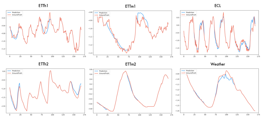
Figure 12: Visualization of imputation results of TimesBERT on six benchmark datasets.

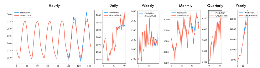
Figure 13: Visualization of short-term forecasting results of TimesBERT on M4 dataset.

References

- Abdulaal et al. (2021) Abdulaal, A., Liu, Z., and Lancewicki, T. Practical approach to asynchronous multivariate time series anomaly detection and localization. KDD, 2021.
- Ansari et al. (2024) Ansari, A. F., Stella, L., Turkmen, C., Zhang, X., Mercado, P., Shen, H., Shchur, O., Rangapuram, S. S., Arango, S. P., Kapoor, S., et al. Chronos: Learning the language of time series. arXiv preprint arXiv:2403.07815, 2024.
- Bagnall et al. (2018) Bagnall, A. J., Dau, H. A., Lines, J., Flynn, M., Large, J., Bostrom, A. G., Southam, P., and Keogh, E. J. The uea multivariate time series classification archive, 2018. arXiv preprint arXiv:1811.00075, 2018.
- Bandaragoda et al. (2018) Bandaragoda, T. R., Ting, K. M., Albrecht, D., Liu, F. T., Zhu, Y., and Wells, J. R. Isolation-based anomaly detection using nearest-neighbor ensembles. Computational Intelligence, 34(4):968–998, 2018.
- Bao et al. (2021) Bao, H., Dong, L., Piao, S., and Wei, F. Beit: Bert pre-training of image transformers. arXiv preprint arXiv:2106.08254, 2021.
- Berndt & Clifford (1994) Berndt, D. J. and Clifford, J. Using dynamic time warping to find patterns in time series. In KDD Workshop, 1994.
- Brown et al. (2020) Brown, T., Mann, B., Ryder, N., Subbiah, M., Kaplan, J. D., Dhariwal, P., Neelakantan, A., Shyam, P., Sastry, G., Askell, A., et al. Language models are few-shot learners. Advances in neural information processing systems, 33:1877–1901, 2020.
- Challu et al. (2023) Challu, C., Olivares, K. G., Oreshkin, B. N., Ramirez, F. G., Canseco, M. M., and Dubrawski, A. Nhits: Neural hierarchical interpolation for time series forecasting. In Proceedings of the AAAI Conference on Artificial Intelligence, volume 37, pp. 6989–6997, 2023.
- Chen et al. (2024) Chen, M., Shen, L., Li, Z., Wang, X. J., Sun, J., and Liu, C. Visionts: Visual masked autoencoders are free-lunch zero-shot time series forecasters. arXiv preprint arXiv:2408.17253, 2024.
- Chen & Guestrin (2016) Chen, T. and Guestrin, C. Xgboost: A scalable tree boosting system. KDD, 2016.
- Das et al. (2023a) Das, A., Kong, W., Leach, A., Sen, R., and Yu, R. Long-term forecasting with tide: Time-series dense encoder. arXiv preprint arXiv:2304.08424, 2023a.
- Das et al. (2023b) Das, A., Kong, W., Sen, R., and Zhou, Y. A decoder-only foundation model for time-series forecasting. arXiv preprint arXiv:2310.10688, 2023b.
- Dau et al. (2019) Dau, H. A., Bagnall, A., Kamgar, K., Yeh, C.-C. M., Zhu, Y., Gharghabi, S., Ratanamahatana, C. A., and Keogh, E. The ucr time series archive. IEEE/CAA Journal of Automatica Sinica, 6(6):1293–1305, 2019.
- Dempster et al. (2020) Dempster, A., Petitjean, F., and Webb, G. I. Rocket: exceptionally fast and accurate time series classification using random convolutional kernels. Data Min. Knowl. Discov., 2020.
- Devlin et al. (2018) Devlin, J., Chang, M.-W., Lee, K., and Toutanova, K. Bert: Pre-training of deep bidirectional transformers for language understanding. arXiv preprint arXiv:1810.04805, 2018.
- Dong et al. (2023) Dong, J., Wu, H., Zhang, H., Zhang, L., Wang, J., and Long, M. Simmtm: A simple pre-training framework for masked time-series modeling. arXiv preprint arXiv:2302.00861, 2023.
- donghao & wang xue (2024) donghao, L. and wang xue. ModernTCN: A modern pure convolution structure for general time series analysis. In The Twelfth International Conference on Learning Representations, 2024. URL https://openreview.net/forum?id=vpJMJerXHU.
- Dosovitskiy et al. (2020) Dosovitskiy, A., Beyer, L., Kolesnikov, A., Weissenborn, D., Zhai, X., Unterthiner, T., Dehghani, M., Minderer, M., Heigold, G., Gelly, S., et al. An image is worth 16x16 words: Transformers for image recognition at scale. arXiv preprint arXiv:2010.11929, 2020.
- Franceschi et al. (2019) Franceschi, J.-Y., Dieuleveut, A., and Jaggi, M. Unsupervised scalable representation learning for multivariate time series. In NeurIPS, 2019.
- Goswami et al. (2024) Goswami, M., Szafer, K., Choudhry, A., Cai, Y., Li, S., and Dubrawski, A. Moment: A family of open time-series foundation models. arXiv preprint arXiv:2402.03885, 2024.
- Gow et al. (2023) Gow, B., Pollard, T., Nathanson, L. A., Johnson, A., Moody, B., Fernandes, C., Greenbaum, N., Berkowitz, S., Moukheiber, D., Eslami, P., et al. Mimic-iv-ecg-diagnostic electrocardiogram matched subset. Type: dataset, 2023.
- Gu et al. (2022) Gu, A., Goel, K., and Ré, C. Efficiently modeling long sequences with structured state spaces. In ICLR, 2022.
- He et al. (2022) He, K., Chen, X., Xie, S., Li, Y., Dollár, P., and Girshick, R. Masked autoencoders are scalable vision learners. In Proceedings of the IEEE/CVF conference on computer vision and pattern recognition, pp. 16000–16009, 2022.
- Hochreiter & Schmidhuber (1997) Hochreiter, S. and Schmidhuber, J. Long short-term memory. Neural Comput., 1997.
- Hundman et al. (2018) Hundman, K., Constantinou, V., Laporte, C., Colwell, I., and Söderström, T. Detecting spacecraft anomalies using lstms and nonparametric dynamic thresholding. KDD, 2018.
- Kitaev et al. (2020) Kitaev, N., Kaiser, L., and Levskaya, A. Reformer: The efficient transformer. In ICLR, 2020.
- Lai et al. (2018) Lai, G., Chang, W.-C., Yang, Y., and Liu, H. Modeling long-and short-term temporal patterns with deep neural networks. In SIGIR, 2018.
- Lan (2019) Lan, Z. Albert: A lite bert for self-supervised learning of language representations. arXiv preprint arXiv:1909.11942, 2019.
- Li et al. (2019) Li, S., Jin, X., Xuan, Y., Zhou, X., Chen, W., Wang, Y.-X., and Yan, X. Enhancing the locality and breaking the memory bottleneck of transformer on time series forecasting. In NeurIPS, 2019.
- Liu et al. (2021) Liu, S., Yu, H., Liao, C., Li, J., Lin, W., Liu, A. X., and Dustdar, S. Pyraformer: Low-complexity pyramidal attention for long-range time series modeling and forecasting. In ICLR, 2021.
- Liu (2019) Liu, Y. Roberta: A robustly optimized bert pretraining approach. arXiv preprint arXiv:1907.11692, 364, 2019.
- Liu et al. (2022) Liu, Y., Wu, H., Wang, J., and Long, M. Non-stationary transformers: Rethinking the stationarity in time series forecasting. In NeurIPS, 2022.
- Liu et al. (2023) Liu, Y., Li, C., Wang, J., and Long, M. Koopa: Learning non-stationary time series dynamics with koopman predictors. arXiv preprint arXiv:2305.18803, 2023.
- Liu et al. (2024a) Liu, Y., Hu, T., Zhang, H., Wu, H., Wang, S., Ma, L., and Long, M. itransformer: Inverted transformers are effective for time series forecasting. arXiv preprint arXiv:2310.06625, 2024a.
- Liu et al. (2024b) Liu, Y., Qin, G., Huang, X., Wang, J., and Long, M. Autotimes: Autoregressive time series forecasters via large language models. arXiv preprint arXiv:2402.02370, 2024b.
- Liu et al. (2024c) Liu, Y., Qin, G., Huang, X., Wang, J., and Long, M. Timer-xl: Long-context transformers for unified time series forecasting. arXiv preprint arXiv:2410.04803, 2024c.
- Liu et al. (2024d) Liu, Y., Zhang, H., Li, C., Huang, X., Wang, J., and Long, M. Timer: Transformers for time series analysis at scale. arXiv preprint arXiv:2402.02368, 2024d.
- Mathur & Tippenhauer (2016) Mathur, A. P. and Tippenhauer, N. O. Swat: a water treatment testbed for research and training on ICS security. In CySWATER, 2016.
- Nie et al. (2023) Nie, Y., Nguyen, N. H., Sinthong, P., and Kalagnanam, J. A time series is worth 64 words: Long-term forecasting with transformers. arXiv preprint arXiv:2211.14730, 2023.
- Oreshkin et al. (2019) Oreshkin, B. N., Carpov, D., Chapados, N., and Bengio, Y. N-BEATS: Neural basis expansion analysis for interpretable time series forecasting. ICLR, 2019.
- Paszke et al. (2019) Paszke, A., Gross, S., Massa, F., Lerer, A., Bradbury, J., Chanan, G., Killeen, T., Lin, Z., Gimelshein, N., Antiga, L., Desmaison, A., Köpf, A., Yang, E., DeVito, Z., Raison, M., Tejani, A., Chilamkurthy, S., Steiner, B., Fang, L., Bai, J., and Chintala, S. Pytorch: An imperative style, high-performance deep learning library. In NeurIPS, 2019.
- Radford et al. (2018) Radford, A., Narasimhan, K., Salimans, T., Sutskever, I., et al. Improving language understanding by generative pre-training. 2018.
- Raffel et al. (2020) Raffel, C., Shazeer, N., Roberts, A., Lee, K., Narang, S., Matena, M., Zhou, Y., Li, W., and Liu, P. J. Exploring the limits of transfer learning with a unified text-to-text transformer. The Journal of Machine Learning Research, 21(1):5485–5551, 2020.
- Spyros Makridakis (2018) Spyros Makridakis. M4 dataset, 2018. URL https://github.com/M4Competition/M4-methods/tree/master/Dataset.
- Su et al. (2019) Su, Y., Zhao, Y., Niu, C., Liu, R., Sun, W., and Pei, D. Robust anomaly detection for multivariate time series through stochastic recurrent neural network. KDD, 2019.
- Van Den Oord et al. (2017) Van Den Oord, A., Vinyals, O., et al. Neural discrete representation learning. Advances in neural information processing systems, 30, 2017.
- Van der Maaten & Hinton (2008) Van der Maaten, L. and Hinton, G. Visualizing data using t-sne. Journal of machine learning research, 9(11), 2008.
- Vaswani et al. (2017a) Vaswani, A., Shazeer, N., Parmar, N., Uszkoreit, J., Jones, L., Gomez, A. N., Kaiser, L., and Polosukhin, I. Attention is all you need. In NeurIPS, 2017a.
- Vaswani et al. (2017b) Vaswani, A., Shazeer, N., Parmar, N., Uszkoreit, J., Jones, L., Gomez, A. N., Kaiser, Ł., and Polosukhin, I. Attention is all you need. Advances in neural information processing systems, 30, 2017b.
- Wang et al. (2022) Wang, H., Peng, J., Huang, F., Wang, J., Chen, J., and Xiao, Y. Micn: Multi-scale local and global context modeling for long-term series forecasting. In The Eleventh International Conference on Learning Representations, 2022.
- Wang et al. (2024) Wang, Y., Wu, H., Dong, J., Liu, Y., Long, M., and Wang, J. Deep time series models: A comprehensive survey and benchmark. 2024.
- Woo et al. (2022) Woo, G., Liu, C., Sahoo, D., Kumar, A., and Hoi, S. C. H. Etsformer: Exponential smoothing transformers for time-series forecasting. arXiv preprint arXiv:2202.01381, 2022.
- Woo et al. (2024) Woo, G., Liu, C., Kumar, A., Xiong, C., Savarese, S., and Sahoo, D. Unified training of universal time series forecasting transformers. arXiv preprint arXiv:2402.02592, 2024.
- Wu et al. (2021) Wu, H., Xu, J., Wang, J., and Long, M. Autoformer: Decomposition transformers with auto-correlation for long-term series forecasting. Advances in neural information processing systems, 34:22419–22430, 2021.
- Wu et al. (2022) Wu, H., Wu, J., Xu, J., Wang, J., and Long, M. Flowformer: Linearizing transformers with conservation flows. In ICML, 2022.
- Wu et al. (2023) Wu, H., Hu, T., Liu, Y., Zhou, H., Wang, J., and Long, M. Timesnet: Temporal 2d-variation modeling for general time series analysis. arXiv preprint arXiv:2210.02186, 2023.
- Xu et al. (2021) Xu, J., Wu, H., Wang, J., and Long, M. Anomaly transformer: Time series anomaly detection with association discrepancy. arXiv preprint arXiv:2110.02642, 2021.
- Zeng et al. (2023a) Zeng, A., Chen, M., Zhang, L., and Xu, Q. Are transformers effective for time series forecasting? 2023a.
- Zeng et al. (2023b) Zeng, A., Chen, M., Zhang, L., and Xu, Q. Are transformers effective for time series forecasting? In Proceedings of the AAAI conference on artificial intelligence, volume 37, pp. 11121–11128, 2023b.
- Zerveas et al. (2021) Zerveas, G., Jayaraman, S., Patel, D., Bhamidipaty, A., and Eickhoff, C. A transformer-based framework for multivariate time series representation learning. In Proceedings of the 27th ACM SIGKDD conference on knowledge discovery & data mining, pp. 2114–2124, 2021.
- Zhang et al. (2022) Zhang, T., Zhang, Y., Cao, W., Bian, J., Yi, X., Zheng, S., and Li, J. Less is more: Fast multivariate time series forecasting with light sampling-oriented mlp structures. arXiv preprint arXiv:2207.01186, 2022.
- Zhou et al. (2021a) Zhou, H., Zhang, S., Peng, J., Zhang, S., Li, J., Xiong, H., and Zhang, W. Informer: Beyond efficient transformer for long sequence time-series forecasting. In AAAI, 2021a.
- Zhou et al. (2021b) Zhou, H., Zhang, S., Peng, J., Zhang, S., Li, J., Xiong, H., and Zhang, W. Informer: Beyond efficient transformer for long sequence time-series forecasting. In Proceedings of the AAAI conference on artificial intelligence, volume 35, pp. 11106–11115, 2021b.
- Zhou et al. (2022) Zhou, T., Ma, Z., Wen, Q., Wang, X., Sun, L., and Jin, R. FEDformer: Frequency enhanced decomposed transformer for long-term series forecasting. In ICML, 2022.
- Zhou et al. (2023) Zhou, T., Niu, P., Wang, X., Sun, L., and Jin, R. One fits all: Power general time series analysis by pretrained lm. arXiv preprint arXiv:2302.11939, 2023.