Department of Computer Science, Royal Holloway, University of London, Egham, UKeduard.eiben@rhul.ac.ukhttps://orcid.org/0000-0003-2628-3435 Algorithms and Complexity Group, TU Wien, Vienna, Austriarganian@gmail.comhttps://orcid.org/0000-0002-7762-8045Projects No. 10.55776/Y1329 and 10.55776/COE12 of the Austrian Science Fund (FWF), Project No. 10.47379/ICT22029 of the Vienna Science Foundation (WWTF) School of Computing, DePaul University, Chicago, USAikanj@cdm.depaul.edu0000-0003-1698-8829 Department of Computer Science, University of Warwick, UKR.Maadapuzhi-Sridharan@warwick.ac.uk \CopyrightEiben et al.
[300]Theory of computation Parameterized complexity and exact algorithms
A Minor-Testing Approach for Coordinated Motion Planning with Sliding Robots
Abstract
We study a variant of the Coordinated Motion Planning problem on undirected graphs, referred to herein as the Coordinated Sliding-Motion Planning (CSMP) problem. In this variant, we are given an undirected graph , robots positioned on distinct vertices of , distinct destination vertices for robots , and . The problem is to decide if there is a serial schedule of at most moves (i.e., of makespan ) such that at the end of the schedule each robot with a destination reaches it, where a robot’s move is a free path (unoccupied by any robots) from its current position to an unoccupied vertex. The problem is known to be NP-hard even on full grids. It has been studied in several contexts, including coin movement and reconfiguration problems, with respect to feasibility, complexity, and approximation. Geometric variants of the problem, in which congruent geometric-shape robots (e.g., unit disk/squares) slide or translate in the Euclidean plane, have also been studied extensively.
We investigate the parameterized complexity of CSMP with respect to two parameters: the number of robots and the makespan . As our first result, we present a fixed-parameter algorithm for CSMP parameterized by . For our second result, we present a fixed-parameter algorithm parameterized by for the special case of CSMP in which only a single robot has a destination and the graph is planar, which we prove to be NP-complete. A crucial new ingredient for both of our results is that the solution admits a succinct representation as a small labeled topological minor of the input graph.
keywords:
coordinated motion planning on graphs, parameterized complexity, topological minor testing, planar graphs1 Introduction
In the coordinated motion planning problem, we are given an integer , an undirected graph , robots positioned on distinct starting vertices of and distinct destination vertices for robots . In each step, one robot (or a subset of robots in other variants of the problem in which robots may move in parallel) may move from its current vertex to an adjacent unoccupied vertex. The goal is to decide if there is a schedule (i.e., a sequence of moves) of length at most , at the end of which each robot has reached its destination vertex without colliding with other robots along the way. The problem and its variants (including the common variant where ) have been extensively studied, with respect to various motion types and graph classes, due to their ubiquitous applications in artificial intelligence (planning), robotics, computational geometry and more generally theoretical computer science [18, 11, 7, 25, 36, 37, 38, 26, 39, 40, 3, 13, 17, 30, 33, 34, 35]. Moreover, it generalizes several well-known puzzles, including Sam Loyd’s famous 15-puzzle—known as the ()-puzzle—and the Rush-Hour Puzzle. Most of these variants are NP-hard, including the aforementioned ()-puzzle [14, 31]. Due to its numerous applications, the coordinated motion planning problem on (full rectangular) grids was posed as the SoCG 2021 Challenge [19].
In this paper, we consider a variant of the coordinated motion planning problem on undirected graphs in which robots move serially one at a time, and a robot’s move consists of a move along a free/unobstructed path (i.e., a path in which no other robot is located at the time of the move) as opposed to a single edge; we refer to such a move as a sliding move, analogous to the type of motion in geometric variants of the coordinated motion planning problem, where robots are geometric shapes (e.g., disks or rectangles) that move by translating/sliding in the plane. These geometric variants have been extensively studied since the 1980s [30, 26, 33, 34, 35]. The goal of this variant is to decide whether there is a schedule of makespan at most , where here the makespan of the schedule is simply the number of moves in it. We denote our general problem of interest as CSMP. We will also consider the special case of CSMP where is planar and —that is, only a designated robot has a destination and the remaining robots merely act as “blockers”. We refer to this special case as Planar-CSMP-1.
Contributions and Techniques.
We present a fixed-parameter algorithm for CSMP parameterized by the number of robots, and a fixed-parameter algorithm for Planar-CSMP-1 parameterized by the makespan , after proving that Planar-CSMP-1 remains NP-hard. A crucial common ingredient for both results is showing that the solution to a problem instance admits a succinct representation, whose size is a function of the parameter, as a topological minor of the input graph. To the best of our knowledge, this is a novel approach in the context of coordinated motion planning problems.
CSMP. Showing that the solution admits a succinct representation entails first bounding the makespan in an optimal solution by a function of the number of robots. Towards this end, we preprocess the graph by shortening (to ) sufficiently long paths comprising degree-2 vertices and focus on two cases. In one case, where the graph has bounded111In the rest of this description, we simply say bounded to refer to values bounded by a function of . treedepth, we show that the instance can be reduced iteratively without altering the solution. This reduction process ultimately results in an instance of bounded size, implying the existence of a solution with a bounded makespan.
In the other case, we use ideas from [11] to define a notion of havens, which are subgraphs of bounded size with the following property: if a robot has to pass through a haven, then with a bounded number of additional steps, we can enable it to pass through the haven regardless of the other robots in the haven (i.e., without collision), effectively “untangling” all the robots’ traversals within the haven. Building on this, we construct a schedule in which each robot interacts with only a bounded number of havens, ultimately leading to a bounded-makespan schedule.
After bounding the makespan in an optimal solution, we show that it essentially describes a graph of bounded size as a topological minor in the input graph. Here, we have to work with rooted topological minors since all robots have specified starting points and some have specified destinations. For us, the roots are just the starting and ending vertices, as we have boundedly-many roots. Towards our goal, we partition the vertices of the graph induced by the edges participating in an optimal solution into two sets: important and unimportant vertices. We show that the number of important vertices is bounded, and that the unimportant vertices form paths whose internal vertices have degree . This structure enables us to show that the graph induced by the edges in the solution (with terminals as roots) is a realization of some rooted graph with a bounded number of vertices as a topological minor in the input graph. We also prove the converse, namely that from any realization of as a topological minor in , one can obtain an optimal solution for the given instance. Towards proving this, we show that if a robot follows a path that is devoid of important vertices, then it slides on that path without stopping. Finally, we leverage known results on topological minor containment to verify the existence of the correct rooted graph.
Planar-CSMP-1. It is easy to see here that the solution admits a succinct representation since the parameter itself is the makespan. The difficulty is that the number of robots in the instance can be very large compared to the parameter , and we cannot find a realization of the succinct solution which avoids the “blocker” robots that do not contribute to the realization. To cope with this hurdle, we exploit the planarity of the graph to reduce its diameter, thus reducing the instance to an instance on a graph with bounded treewidth. The fixed-parameter tractability of the problem will then follow from Courcelle’s Theorem [9, 2].
The heart of our reduction method is finding an “irrelevant edge” in the graph that can be safely contracted to produce an equivalent instance of the problem. While the method of finding an irrelevant edge and contracting it has been employed in several results in the literature to exclude large grids, thus reducing the treewidth of the graph, in our setting the grid approach seems unworkable. Instead, we show that a sufficiently-large component of free vertices (i.e., vertices with no blockers on them) must contain an irrelevant edge. We reduce all the cases to one where is formed by a skeleton consisting of a “long” path of degree-2 vertices (the degree is taken in ), plus a “small” number of additional vertices. We then show that if the instance is a YES-instance of the problem, then it admits a solution that interacts nicely with this skeleton, in the sense that we can identify a subgraph of the representation of the solution, i.e., a topological minor that is essentially a roadmap of the solution, separated from the rest of the solution by a small cut. We can enumerate each possible representation of the part of the solution that interacts with the skeleton, and for each possible representation, test whether it exists near the skeleton; if it does, we mark the vertices in the graph that realize this representation. Since the skeleton is long, the total number of marked vertices on the skeleton is small, and an edge with both endpoints unmarked—and hence can be contracted—must exist.
Related Work.
The CSMP problem, with , has been studied in [8] on several graph classes, and with respect to various settings, based on whether or not the destinations of the robots are distinguished (referred to as labeled or unlabeled). The graph classes that were considered include trees, grids, planar graphs, and general graphs, and it was shown that the problem is NP-hard even for (full rectangular) grids. Upper and lower bounds on the makespan of a solution, as well as computational complexity and approximation results, were derived for the various settings considered in [8].
A related problem to CSMP is that of moving unit disks (or objects [17]) in the plane, which has been studied in the context of reconfiguring/moving coins in the plane [1, 4], and was shown to be NP-hard [1]. We also mention the related work on coordinated pebble motion on graphs (and permutation groups), which was studied in [27] motivated by the work on the ()-puzzle.
The variant of coordinated motion planning in which only one designated robot is required to reach its destination, that is , and each move is along a single edge, was studied as Graph Motion Planning with 1 Robot in [29], where complexity and approximation results were derived.
Despite the tremendous amount of work on coordinated motion planning problems, not much work has been done from the parameterized complexity perspective. The work in [11] studied the parameterized complexity of the non-sliding version of CSMP, that is, where each motion step is along a single edge, parameterized by the makespan in the serial setting. Another recent work [18] studied the parameterized complexity of the classical coordinated motion planning problem on grids, presenting parameterized algorithms for various objective measures (makespan, travel length). The work in [21] established the W[1]-hardness of the classical coordinated motion planning problem parameterized by the makespan in the parallel motion setting, and also showed the NP-hardness of this problem on trees, among other results. Finally, the parameterized complexity of a geometric variant of the PSPACE-complete Rush-Hour problem, which itself was shown to be PSPACE-complete [22], was studied [20]; in particular, that problem was shown to be FPT when parameterized by either the number of robots (i.e., cars) or the number of moves.
2 Terminology and Problem Definition
Graphs.
For a graph , denotes the set of all simple paths in . The length of a path is the number of edges in it. For a path and vertices in it, we denote by the subpath of starting at and ending at . The -distance between and , denoted , is the length of .
Parameterized Complexity.
A parameterized problem is a subset of , where is a fixed alphabet. Each instance of is a pair , where is called the parameter. A parameterized problem is fixed-parameter tractable (FPT) [10, 16, 23], if there is an algorithm, called a fixed-parameter algorithm or an FPT-algorithm, that decides whether an input is a member of in time , where is a computable function and is the input instance size. The class FPT denotes the class of all fixed-parameter tractable parameterized problems.
Treewidth is a fundamental graph parameter which can be seen as a measure of how similar a graph is to a tree; trees have treewidth , while the complete -vertex graph has treewidth . A formal definition of treewidth will not be necessary to obtain our results; however, we will make use of the fact that every planar graph with diameter has treewidth at most [32, 5] and of Courcelle’s Theorem (introduced below).
Monadic Second Order Logic.
We consider Monadic Second Order (MSO) logic on edge- and vertex-labeled graphs in terms of their incidence structure, whose universe contains vertices and edges; the incidence between vertices and edges is represented by a binary relation. We assume an infinite supply of individual variables and of set variables . The atomic formulas are (“ is a vertex”), (“ is an edge”), (“vertex is incident with edge ”), (equality), (“vertex or edge has label ”), and (“vertex or edge is an element of set ”). MSO formulas are built up from atomic formulas using the usual Boolean connectives , quantification over individual variables (, ), and quantification over set variables (, ).
Free and bound variables of a formula are defined in the usual way. To indicate that the set of free individual variables of formula is and the set of free set variables of formula is we write . If is a graph, and we write to denote that holds in if the variables are interpreted by the vertices or edges , for , and the variables are interpreted by the sets , for .
The following result (the well-known Courcelle’s theorem [9]) shows that if has bounded treewidth [32] then we can find an assignment to the set of free variables with (if one exists) in linear time.
Proposition A (Courcelle’s Theorem [9, 2]).
Let be a fixed MSO formula with free individual variables and free set variables , and let be a constant. Then there is a linear-time algorithm that, given a labeled graph of treewidth at most , either outputs and such that or correctly identifies that no such vertices and sets exist.
Rooted graphs.
A rooted graph is a graph where some vertices are labeled—formally:
Definition 2.1 (Rooted graphs).
A rooted graph is a graph with a set of distinguished vertices called roots and a labeling . The set is the root set of , and the label set of is .
Definition 2.2 (Topological minors of rooted graphs [24]).
Let and be two rooted graphs with labelings and for their root sets. We say that is a topological minor of if there exist injective functions and such that
-
•
for every , the endpoints of are and ,
-
•
for every distinct , the paths and are internally vertex-disjoint,
-
•
there does not exist a vertex in the image of and an edge such that is an internal vertex on , and
-
•
for every , .
We say that is a realization of as a topological minor in . Moreover, the subgraph of induced by the union of the edges in the paths in for and the vertices in for is called a topological minor model of .
Note that if , then the above coincides with the usual definition of topological minors.
Proposition 2.3.
([24]) There is an algorithm that, given two rooted graphs and , runs in time for some computable function and decides whether is a topological minor of .
Remark 2.4.
Although the algorithm in Proposition 2.3 is for the decision version of the problem, a realization if one exists, can be computed using self-reducibility arguments as follows. By iteratively deleting an edge of and running the algorithm of Proposition 2.3, we can identify a minimal subgraph of that is a subdivision of . Isolated vertices of can be mapped to isolated vertices of in an arbitrary way. The number of vertices of of degree at least three is bounded by , and the mapping of these to can be guessed. Moreover, the number of maximal paths in that only have degree-2 vertices as internal vertices (call this set ) must be bounded by a function of , and we can guess the mapping of vertices of of degree at most 2 into and the final verification step is straightforward brute force.
Definition B (Forest embedding and treedepth).
A forest embedding of a graph is a pair , where is a rooted forest and is a bijective function, such that for each , either is a descendant of , or is a descendant of . The depth of the forest embedding is the number of vertices in the longest root-to-leaf path in . The treedepth of a graph , denoted by , is the minimum over the depths of all possible forest embeddings of .
If is connected, then the forest embedding of consists of a single tree, i.e., it is a tree embedding.
Proposition C ([28]).
If a graph has no path of length at least , then it has treedepth at most .
Observation D.
Let be a graph with a forest embedding and consider some vertex . If the number of children of in is at least and denotes the set of vertices appearing in the root-to- path in the tree of containing , then the number of connected components of is at least .
Proof 2.5.
By the definition of forest embeddings, (i) every descendant of in is adjacent in to either another descendant of in or a vertex in and (ii) descendants of distinct children of in are non-adjacent in .
Problem Formalizations.
In our problems of interest, we are given an undirected graph and a set of robots where is partitioned into two sets and . Each , has a starting vertex and a destination vertex in and each is associated only with a starting vertex . We refer to the elements in the set as terminals. We assume that all the are pairwise distinct and that all the are pairwise distinct. We use a discrete time frame , , to reference the sequence of moves of the robots. In each time step , exactly one robot moves and the rest remain stationary.
In Coordinated Sliding-Motion Planning (CSMP), we are given a tuple , where and are as described in the last paragraph and . The goal is to decide whether there is a sequence of moves such that robots move serially one at a time, where a robot’s move consists of a move along a free/unobstructed path (i.e., a path in which no other robot is located at the time of the move), and such that each starts in at time step and each is positioned on at the end of time step . The second problem that we consider is a restriction of CSMP to the case where is planar and contains exactly one robot, referred to as the main robot. We refer to this restriction as Planar-CSMP-1, and for simplicity represent its instances as tuples of the form , where and are the starting and destination vertices of the main robot, respectively, and is the set of all robots.
We next introduce some notation that will be used in our technical sections. A route for robot is a tuple where each is a vertex in and each is a simple path in , such that (i) and if and (ii) , is a - path in (if , then is the singleton path comprising the same vertex).
Put simply, each corresponds to a “walk” in . If vertices of at two consecutive time steps and are identical, then is a waiting time step for the robot . Moreover, each begins at its starting vertex at time step , and if then is at its destination vertex at time step . Though we work with undirected graphs and the paths described above are undirected paths, each path has a natural starting vertex and ending vertex designated by the time step .
Definition 2.6.
Two routes and , where , are non-conflicting if , the path is disjoint from and the path is disjoint from . Otherwise, we say that and conflict.
In particular, in the above definition, for every and , . Intuitively, two routes conflict if the corresponding robots are at the same vertex at the end of a time step, or one “hits” the other while traveling along a path during some time step. A schedule S for is a set of pairwise non-conflicting routes , during a time interval , where exactly one robot moves in each time step. The number of moves in a route or the number of moves of its associated robot is the number of time steps such that . The total number of moves (or makespan) in a schedule is the sum of the number of moves in its routes. A schedule of minimum total moves is called an optimal schedule.
A vertex is occupied at time step if some robot is located at at time step ; otherwise, is said to be free (or unoccupied). If the time step is not specified, it is assumed to be time step (i.e., in the initial state). At each time step, a robot may either move to a different vertex, or stay at its current vertex. Finally, we always assume that the input graph is connected since otherwise, we can work on individual connected components.
Remarks on Feasibility and Constructiveness.
When only considering feasibility, CSMP is equivalent to the version where each move is along a single edge instead of an unobstructed path.
Hence, by the result of Yu and Rus [41] (observed to be extendable to the setting where not every robot has a destination [11]), it follows that it is linear-time solvable.
Proposition E (Implied by [41]).
The existence of a schedule for an instance of CSMP can be decided in linear time. Moreover, if such a schedule exists, then a schedule with moves can be computed in time.
Proposition E implies inclusion in NP, and allows us to assume henceforth that every instance of CSMP is feasible (otherwise, in linear time we can reject the instance).
We note that even though CSMP is formalized as a decision problem, all the algorithms provided in this paper are constructive and can output a corresponding schedule (when it exists) as a witness.
3 FPT Algorithm for CSMP Parameterized by the Number of Robots
In this section, we show that CSMP is FPT parameterized by the number of robots in the input. Note that we do not assume any restrictions on the input graph.
Our strategy has three high-level steps: (i) We first show that if a solution exists, then there is an optimal schedule whose makespan is bounded222We recall that by bounded, we mean “bounded by a function of the parameter”—in this case, .. (ii) We then show that such a solution is essentially a realization of a rooted graph of bounded size as a topological minor in a rooted graph obtained by assigning unique labels to the terminals in . We also prove the converse, that is, from any realization of as a topological minor in , one can obtain an optimal solution for the given instance. (iii) Finally, we leverage known results on topological minor containment to verify the existence of the correct rooted graph. Let us now give more detail on Steps (i) and (ii).
Step (i): To prove the existence of a solution with boundedly many moves, we preprocess the graph by applying a reduction rule that shortens degree-2 paths to a bounded length. This simplification allows us to focus on two cases for the graph (assuming it is connected):
Case (a): Bounded Treedepth. If the graph has bounded treedepth, we show that instances with bounded treedepth and a bounded number of robots can be reduced iteratively without altering the solution. This reduction process results in an instance of bounded size, implying the existence of a solution with a bounded makespan.
Case (b): Long Paths. Suppose every vertex is the endpoint of a sufficiently long path. We use ideas from [11] to define a suitable notion of havens for our setting; in particular, havens are subgraphs of bounded size that can efficiently handle collisions. Here, by the “efficient handling” of collisions, we mean that given any pair of “configurations” of robots in a haven, we can move the robots from one configuration to another without any conflicts using only boundedly many moves. Thus, with a small number of time steps, a robot can pass through a haven without collision, regardless of other robots in the haven. Building on this fact, we construct a schedule where each robot interacts with only a bounded number of havens. Within each haven, the number of moves used by a robot is bounded and we show that outside the havens, the robot only makes boundedly many moves as well. This yields a bound on the makespan of the schedule.
Step (ii): Consider the graph induced by the edges in the solution. We partition the vertices of this graph into two sets: important and unimportant vertices. The important vertices are those with degree at least three, the terminals, and any vertex where a robot waits at any time step. We show that the number of important vertices is bounded by a function of (say, ). Moreover, by definition, the unimportant vertices form paths with only degree-2 vertices as internal vertices. Additionally, every robot that visits a vertex in such a path slides without stopping on any vertex of this path. This structure enables us to show that the graph induced by the edges in the solution (with terminals as roots) is a realization of some rooted graph with at most vertices as a topological minor in the input graph.
3.1 Bounding the Makespan in an Optimal Schedule
Our first task is to apply a reduction rule to the given instance that enforces useful structural properties on the graph without affecting the existence of a solution.
Reduction Rule 1.
Let be an instance of CSMP. If there is a path in such that every internal vertex of is disjoint from the set of terminals and has degree exactly two in , then shorten to length .
Lemma F.
Let be an instance of CSMP and be the instance obtained by applying Reduction Rule 1. These two instances are equivalent, that is, has a solution if and only if has a solution.
Proof 3.1.
Consider a maximal path in such that every internal vertex has degree exactly two in and has no terminal as an internal vertex. Suppose that has more than internal vertices and let and be its endpoints. Let denote the shortened - path with which we replaced . Let denote the instance resulting from applying the reduction rule. For each endpoint of , let denote the internal vertices of closest to . It is straightforward to see that if has a solution, then so does . Conversely, we consider a schedule for and produce a schedule for with at most the same number of moves as S. The idea is to ensure that at any time step, (i) the robots waiting on the path are the same as those waiting on , and (ii) the relative ordering of the robots waiting on the path is the same as their relative ordering on the path . Here, by the relative ordering of the robots on a path, we refer to the permutation of robots that gives their ordering in terms of increasing distance along from the endpoint whose identifier is lexicographically the smaller. This is ensured by considering the following four cases and constructing accordingly.
-
•
If there is a time step in the schedule S during which a robot enters through one of the endpoints of and exits through the other, then the same movement is captured in by passing through the entirety of .
-
•
Next, consider a time step where robot enters through the endpoint and waits on an internal vertex of . Recall that is the position of robot at the end of time step . Then, formally, we have that is not in , is an internal vertex of and the path contains . Then, in time step of , we let enter through and make it wait at the vertex of that is farthest from among all vertices of that do not have a robot waiting on them. Since has size and by our strategy, robots occupy starting from the farthest available vertex from , it follows that every robot that needs to wait on in this way always has an available vertex.
-
•
Next, consider a time step where robot exits the path through an endpoint after waiting on an internal vertex at time step . Formally, is in , is not in and the path contains . Then, we move robot to and then follow the rest of the path as given by S.
-
•
Finally, consider the case where a robot moves from one internal vertex of to another. In this case, we do not need to make a move in since we trivially maintain both the subset of robots on and their relative ordering.
In every case, assuming that the relative ordering of the robots on and is the same at time step , it follows that the specified moves are possible and moreover, we ensure that the relative ordering of the robots on the paths and is the same at the end of time step (in particular, the subset of robots on both paths is the same). Moreover, by construction of , we have also ensured that a vertex disjoint from has robot on it at time step in schedule S if and only if the same happens in schedule . This ensures that has at most the same number of moves as S and no pair of routes in conflict, completing the proof.
We say that an instance is irreducible if Reduction Rule 1 cannot be applied. In the rest of this section, we work with such instances. Our goal now is to show that every YES-instance has a schedule in which the makespan is bounded by a function of the number of robots. Specifically, we prove the following fact.
Lemma 3.2.
Let be an instance of CSMP. If is a YES-instance, then has an optimal schedule with moves.
The proof strategy of Lemma 3.2 is as follows. We show that for a YES-instance, either the treedepth of the input graph is bounded or a certain locality property holds (roughly speaking, every vertex is sufficiently close to a vertex of degree at least three). We then show that in either case, there is a solution with boundedly-many moves. Specifically, when the treedepth is bounded, we show how to reduce the graph to a bounded-size graph without affecting the existence of a solution (thus implicitly bounding the makespan of an optimal solution) and otherwise, we show how the aforementioned locality property can be used along with a greedy strategy to produce a schedule with boundedly many moves (again, bounding the makespan of an optimal solution).
Towards the proof of Lemma 3.2, we adapt ideas from [11] on the notion of “havens” that was originally designed to address conflicts occurring in schedules for CSMP instances where every move is required to be along a single edge.
Definition G.
For and graph , a vertex is a -anchor if it has degree at least three in and lies on a path of length . This path is called a -haven anchored at . We also say that is a -haven for a vertex if lies on and has -distance at least and at most from the anchor . Additionally, we say that is a strong -haven anchored at if it is a -haven anchored at for both endpoints of .
Roughly speaking, a strong -haven for a vertex anchored at a vertex of degree at least three is a path of length starting at and containing such that is approximately in the middle of the path. If depends only on , then such a path can be viewed as being short enough to allow local modifications in the schedule within the path at a relatively low cost. At the same time, since is sufficiently far from either endpoint, it allows ample room on either side of to place all the robots if necessary. This property will prove to be useful in subsequent arguments.
Lemma H.
In an irreducible instance , either the treedepth of is or, for every vertex , there is a path and a vertex such that (i) is one of the endpoints of and (ii) is a strong -haven anchored at , where .
Proof 3.3.
Fix some with the precise value to be determined later. If has no path of length , then by Proposition C, the treedepth of is bounded by .
Otherwise, consider a path of length and pick a vertex . Let be a path from to an arbitrary vertex in . Notice that the union of and contains a - path of length exactly for some vertex . Divide into three equally-long subpaths starting from : , , . Due to the fact that there are at most terminals, it follows that either contains a vertex with degree at least three in , or it contains at least one subpath of length at least that has only degree-2 vertices as internal vertices. However, by irreducibility, we have that . By choosing , we infer that contains a vertex of degree 3, which we set as the required vertex and the path as the path claimed in the lemma statement.
The following lemma describes the reduction procedure that ultimately enables us to reduce any sufficiently large graph of low treedepth without affecting a solution.
Lemma I.
Consider an instance and a vertex set in of size at most . If the number of connected components of is greater than , then there is a connected component in such that is a YES-instance if and only if is a YES-instance.
Proof 3.4.
The proof idea is as follows. If the premise of the lemma is satisfied, then there exists a set of connected components of such that for every . At most of the components in contain terminals. Hence, we may assume without loss of generality that the components in do not contain terminals. Call these components, exceptional components, and the vertices in them exceptional vertices.
We then argue that removing the component does not affect the existence of a solution. To do so, we show that an optimal schedule for can be modified in such a way that if robot interacts with the exceptional vertices (so, in particular, the component ), it is instead re-routed through the component and stays disjoint from the remaining exceptional components. In this way, by ensuring that is ‘reserved’ for the exclusive use of robot , we argue that there are no conflicts caused by our re-routing. The formal argument follows.
Let . It is clear that if is a YES-instance, then so is . So, let us consider the converse and take an optimal schedule for . Our goal is to produce a schedule for with no more moves than in S. For robots that do not visit an exceptional vertex, the route in is set to be the same as that in S. If no exceptional component is ever visited by any robot in the schedule S, then we are done. So, assume that this is not the case. For every ], let be the first time step during which robot visits an exceptional component and let be the last time step during which robot visits an exceptional component. Notice that and need not exist for every robot . However, if exists for a robot that has a destination, then also exists since no terminals are present in any component in .
We now describe how route is modified for a robot for which time step exists. Let the path be an - path for vertices and . We consider the following two scenarios based on the first interaction of robot with the exceptional components. By the definition of , it must be the case that is not an exceptional vertex.
-
1.
Suppose that is not an exceptional vertex. That is, in time step , robot simply ‘passes through’ the exceptional vertices without waiting on any of them. Let and be vertices of the set that appear on this path right before the first occurrence of an exceptional vertex and right after the last occurrence of an exceptional vertex, respectively. We then modify by removing the - subpath and replacing it with an - path that has all internal vertices in . The required - path exists since every exceptional component has the same neighborhood. Moreover, as long as we ensure that no other robot visits a vertex of , this does not create a conflict.
-
2.
Suppose that is an exceptional vertex. That is, at the end of time step , robot waits at an exceptional vertex. Let be the vertex of that appears on right before the first occurrence of an exceptional vertex. Then, we replace the - subpath with an - edge where is an arbitrary neighbor of in . We then consider two subcases:
-
(a)
If does not exist, it must be the case that does not have a destination and so, we never move again.
-
(b)
Otherwise, consider the path using which robot leaves the exceptional components for the final time. Let be the last occurrence of an exceptional vertex in this path. Then, in , replace the subpath from the starting vertex up to with an arbitrary path from to that has all vertices except inside , which must exist since all exceptional components have the same neighborhood.
As long as we ensure that in , no other robot visits a vertex of , these operations do not create a conflict.
-
(a)
It follows from the construction that if does not exist, then the route of the robot will be the same in S and . More generally, at any time step , robot and vertex that is not exceptional, robot is on vertex at the end of time step in S if and only if the same happens in . This also implies that the number of moves in is no more than the number of moves in S. Finally, since our construction ensures that in , robot only visits components among the exceptional components, we do not create conflicts by our re-routing.
Lemma J.
If is a YES-instance, then it has a schedule with at most steps.
Proof 3.5.
We begin by exhaustively enumerating every set in of size at most . For those sets of size such that the number of connected components of is greater than , remove the ‘irrelevant’ component given by Lemma I. Note that we do not care about the algorithmic efficiency of this operation as the lemma statement asserts the existence of a certain schedule and not the efficient computability of this schedule. Moreover, removing a vertex does not increase the treedepth of a graph and so, we conclude that when this reduction is no longer applicable, the graph, , also has treedepth at most . Finally, recall that we work on a connected graph and notice that is also connected and by Lemma I, since is a YES-instance, so is the instance induced by .
We claim that the number of vertices in is bounded by . Consider the tree embedding of . If every vertex has at most children, then we are done since the depth of the tree embedding is at most . Suppose that there is a vertex that has more than children in the forest embedding. Let be the set of vertices on the root-to- path in the embedding. Notice that has size at most . Let denote all the connected components of . By Observation D, it follows that has size more than , which is a contradiction to the fact that cannot be reduced further.
Finally, we use the fact that every feasible instance on a graph with vertices has a schedule with steps (Proposition E) to conclude that has a schedule with steps.
Since Lemma J achieves our objective of bounding the size of the optimal schedule when the graph has bounded treedepth, we next focus on the case where Lemma H is only able to guarantee that for every vertex , there is a -haven for anchored at some vertex , where .
For a set of robots and a subgraph , a configuration of w.r.t. is an injection . We show using a lemma of Deligkas et al. (Lemma 10, [11], see arXiv version [12] for the proof) that we can move the robots in a -haven from any configuration to any other configuration within the same haven, using a total of moves.
Lemma K (Slightly modified statement of Lemma 10, [11]).
Consider a vertex and three connected subgraphs of such that: (i) the pairwise intersection of the vertex sets of any pair of these subgraphs is exactly , and (ii) , , and . Let denote the subgraph of induced by the vertices in whose distance from in is at most . Then for any set of robots in with current configuration , any configuration with respect to can be obtained from via a sequence of moves that take place in .
Note that in Lemma K as stated in [11], each move is along a single edge. However, in this paper we allow moves along unobstructed paths, so the number of moves given by their lemma is an upper bound for us as well. Moreover, upon examining their statement and proof, we find that the value of used in [11] was and hence the lemma simply gave an upper bound of on the number of moves, but we will set to be a value that is quadratic in , hence we have restated the lemma to account for this.
Lemma L.
Let be a strong -haven anchored at some vertex , where . Then, there exist three connected subgraphs of such that: (i) the pairwise intersection of the vertex sets of any pair of these subgraphs is exactly , and (ii) , , and , and (iii) and (iv) every vertex has distance from in the graph induced by .
Proof 3.6.
Say that is an - path. Since is a strong -haven anchored at , it must be the case that has distance to both and . Let and denote the neighbors of on , with chosen as the one that is closer to .
Since has degree at least three, there is a neighbor of that is distinct from and . If is not in , then we are done by choosing and to be the two subpaths from to the two endpoints of and choosing to be the graph comprising the edge . Otherwise, lies on . Assume without loss of generality that lies between and . Then, also lies between and . Then, set to be the subpath . Set to be the graph comprising the edge and set to be the graph .
This completes the proof of the lemma.
For a strong -haven anchored at some vertex , we denote by , the graph obtained by taking the union of and an arbitrarily chosen set of three edges incident on .
Lemma M.
Let be a strong -haven anchored at some vertex , where . For any set of robots in with current configuration , any configuration with respect to can be obtained from via a sequence of moves that take place in .
Proof 3.7.
A connected subgraph is called an -meta-haven if it is obtained by taking the union of the edges of , where each is a strong -haven anchored at . A straightforward consequence of Lemma M is the following.
Lemma N.
Let be an -meta-haven, where and . For any set of robots in with current configuration , any configuration with respect to can be obtained from via a sequence of moves that take place in .
We are now ready to complete the proof of the main lemma of this subsection. Let us restate it here.
See 3.2
Proof 3.8.
If has treedepth bounded by , then invoking Lemma J with this bound on the treedepth, we conclude that if is a YES-instance, then it has a schedule with moves.
Otherwise, Lemma H guarantees that for every vertex , there is a -haven for anchored at some vertex , where . Moreover, is a strong -haven and has as one of its endpoints. The proof idea from here onwards is similar to that of Eiben et al. (Theorem 15, [11]). However, we have defined our notion of havens in such a way that our arguments are simpler. Assume without loss of generality that is a robot with a destination. Let us now describe a sequence of moves that take from to . The complete schedule then repeats the same strategy for subsequent robots, giving us a bound of moves in total.
For every terminal , fix to be a strong -haven that has as one of its endpoints. Let denote meta-havens defined by , where is a terminal. By ensuring that each is inclusion-wise maximal, we guarantee that and are disjoint for .
Let denote a walk from to in . In the traversal of from to , let and denote the first and last vertices, respectively, that belong to some meta-haven, say . Then, we replace the subwalk from to with a walk given by Lemma N, which takes moves. The other robots currently in the meta-heaven can be moved arbitrarily to other positions inside it. So, the only requirement of the configuration with which we invoke Lemma N is that starts in and ends in . By doing this once for every meta-haven, we obtain a route for that enters and exits each meta-haven at most once and takes moves inside each meta-haven. Hence, we obtain a route for that takes moves overall.
3.2 Succinct Representation of a Solution
In what follows, fix an optimal schedule for an instance . By Lemma 3.2, we may assume, without loss of generality, that S has length . We also assume that no robot moves in two consecutive time steps since otherwise, the movements of such a robot could be done in a single time step while the remaining robots wait. Moreover, we say that an edge of is traversed by S if there is an and a time step such that the path contains the edge . That is, some robot uses the edge in some time step . We denote by , the subgraph of induced by the edges traversed by S. For a time step , we denote by the subgraph of induced by the edges traversed by S up to time step . A vertex in is a waiting vertex within time interval if there is a robot and a time step such that is at at time steps and . We say that is a waiting vertex if it is a waiting vertex within some time interval. A vertex in is an intersection vertex within time interval if its degree in is at least three. We say that is an intersection vertex if it is an intersection vertex within some time interval. A vertex in is an important vertex within time interval if it is either a terminal vertex, or within time interval it is a waiting vertex or an intersection vertex. Otherwise, is unimportant within time interval . We say that is an important (unimportant) vertex if it is important (resp. unimportant) within some time interval.
The number of waiting vertices within time interval is at most .
Proof 3.9.
Initially, the robots are on terminals and in every time step, exactly one robot moves to a (potentially new) waiting vertex while the remaining robots remain stationary.
The unimportant vertices within any time interval induce a disjoint union of paths and any endpoint of any of these paths has degree 2 in .
Proof 3.10.
Every vertex of degree at least three in is important within this time interval.
For a time step , we denote by , the set of all - paths of non-zero length such that and are distinct important vertices within time interval and every internal vertex of is an unimportant vertex within time interval .
For two paths and in , their crossing points are those vertices that have degree at least three in the graph induced by the edges in .
We say that S is a special schedule up to time step if, for every robot and such that moves in time step , the path has at most four crossing points with any path in where . Note that every schedule is trivially special at time step 1 since only a single path has been taken at this point. Moreover, has size at least one because a move has been made and so, has size at least one for every . We say that S is a special schedule if it is a special schedule up to the final time step.
We say that two schedules are equivalent at time step if the positions of all the robots at the end of time is the same in both schedules, that is, robot is on vertex after time step in one schedule if and only if the same happens in the other schedule. We say that two schedules are equivalent if they are equivalent at every time step. In particular, two equivalent schedules take the same number of time steps.
Lemma 3.11.
There is a solution that is a special schedule.
Proof 3.12.
We start with the schedule S and suppose that it has time steps. Let be a schedule that is equivalent to S and let be the maximum time step such that is a special schedule up to time step . We choose so that is maximized. As observed above, . Since we are done otherwise, we assume that . Now, let .
Suppose that moves in time step using the path . By our choice of (and by extension, ) it must be the case that some path in and have more than four crossing points. Along the traversal of from to , let the second and third crossing points be and , respectively. Then, we can replace the subpath with the subpath to obtain an alternate schedule that is equivalent to S and with fewer crossing points. In fact, by doing the same for every path in that has more than two crossing points with , we obtain a schedule that is equivalent to S and which is also special up to time step , a contradiction to our choice of . This completes the proof of the lemma.
Henceforth, we assume that the solution S is a special schedule.
Lemma 3.13.
The number of important vertices in is bounded by .
Proof 3.14.
Let denote the set of waiting vertices in and let denote the set of intersection vertices in that are not terminals or waiting vertices. Note that all but at most two of the terminals are by definition, waiting vertices. So, the number of important vertices is bounded by .
By Observation 3.2, since the total number of moves in S is at most (which also bounds the number of time steps in S), the number of waiting vertices in is at most . Therefore, it suffices to bound the size of . Let denote the subset of that is important within time interval . Clearly, . Notice that every vertex in is either a crossing point of the path with some path in or the endpoint of that is distinct from . By Lemma 3.11, we have that has at most four crossing points with any path in . Hence, we have that is at most . Moreover, since each path in gets split into at most five parts by the crossing points, we have that . For simplicity, let us bound by since is always non-empty. This implies that and hence, is at most . This gives us the required bound of on the size of and since , completes the proof of the lemma.
3.3 Leveraging Succinct Representations and Topological Minor Containment
In what follows, fix a schedule for an instance .
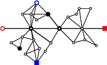
We define the representation of S to be the rooted graph (denoted by ) whose vertices are the important vertices of , and in which there is an edge between two vertices and if and only if there is a - path in whose internal vertices have degree 2 in and are unimportant. Moreover, the terminals receive unique labels (assume that the terminals are labeled with for some ) and the remaining vertices receive the same label which is distinct from those of the terminals, say . An illustration is provided in Figure 1. From Lemma 3.13, we directly obtain:
Lemma 3.15.
If a solution exists, then there is a solution whose representation has vertices.

For the input graph , we let denote the rooted graph where the terminals get their unique labels and the rest of the vertices get a specific label , where is the number of terminals.
Lemma 3.16.
is a topological minor of and moreover, any realization of as a topological minor in implies a schedule with length at most that of S.
Proof 3.17.
The forward direction is obvious and follows from the construction of .
Consider the converse direction. Notice that it is straightforward to interpret S as a schedule on the graph since the edges of correspond to paths of with no waiting vertices. Let be a realization of as a topological minor in . We now define a schedule where each . For every and time step , . Moreover, for and time step , if is a path with at least one edge then, is obtained by concatenating the paths in the natural way. The resulting schedule is equivalent to S by construction and comprises mutually non-conflicting routes since S is non-conflicting.
Theorem 3.18.
CSMP is fixed-parameter tractable parameterized by the number of robots.
Proof 3.19.
For a hypothetical optimal solution S, we guess (i.e., use brute-force branching to determine) the representation . By Lemma 3.15, there are at most choices for some and these can be enumerated in FPT time. For each guess , we do the following:
-
1.
Decide whether the guess is feasible by brute-forcing over it. More precisely, we guess the configurations of the robots at each time step and verify that this guess corresponds to a set of non-conflicting routes with at most moves in total. Note that we can assume that no configuration repeats.Reject guesses that do not pass this check. Clearly, this step takes time for some computable function .
-
2.
For each guess that is not rejected, invoke Proposition 2.3 to decide whether is a topological minor of and return “yes” if and only if at least one of the invocations returns “yes”.
4 An FPT Algorithm for Planar-CSMP-1 Parameterized by the Makespan
We start this section by showing that Planar-CSMP-1 is NP-complete. The reduction is an adaptation of a reduction in [8] for showing the NP-hardness of a chip reconfiguration problem on grids:
Theorem 4.1.
Planar-CSMP-1 is NP-complete.
Proof 4.2.
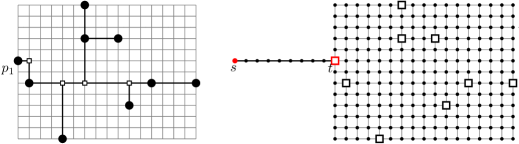
It is straightforward to see that the problem is in NP. To show its NP-hardness, we slightly modify the reduction in [8], which was used to prove the NP-hardness of a related chip/coin moving problems on grids. In fact, we will show that the slice of the problem that consists of the restriction to instances in which the underlying graph is a subgrid (i.e., a subgraph of a rectangular grid), is NP-hard. We closely follow the notations used in [8], and refer to Figure 2 for illustration.
The reduction is from the Strongly NP-hard problem Rectilinear Steiner Tree (RST) [GareyJohnson]. An instance of RST consists of a set of points called terminals. Without loss of generality, we will assume that is a leftmost point in and that its -coordinate is zero. Since RST is Strongly NP-hard, we can assume that all points in have integer coordinates and are encoded in unary. We are also given an integer , and the problem is to decide whether there is a Steiner tree, each of whose edges is either a horizontal or a vertical line segment, that connects all points in and such that the sum of the (Euclidean) lengths of its edges is at most .
To produce an instance of Planar-CSMP-1, we choose the smallest rectangular bounding box that encloses the points in , and we construct a grid graph whose vertices are the points having integer coordinates in (including its boundaries). Observe that, we may assume that if the instance of RST has a solution, then it has a solution that is completely contained in . Now we add to a path of new vertices that all lie on the same horizontal line as , and such that the -coordinate of is , and the -coordinate of is , for . We add the edge , thus connecting the path to via . This completes the construction of the plane graph , which is a subgrid, in the instance of Planar-CSMP-1. The main robot in the instance is located at and its destination is . All vertices of other than and the terminals are occupied by robots. Clearly, the instance of Planar-CSMP-1 can be constructed in polynomial time.
We prove the following claim (similar to the claim in Theorem 3.1 in [8]), which establishes the correctness of the reduction: The instance of RST has a rectilinear Steiner tree of length at most if and only if the instance of Planar-CSMP-1 has a solution that uses at most moves.
To prove the direct implication, let be a solution to the instance of RST. Form the rooted tree by adding to the path , and rooting at . We now apply the following process until eventually is located at . We choose any leaf of that is unoccupied at this point; we choose a closest (w.r.t. distance in ) occupied ancestor to , move it to along , and remove from . Note that all the initially unoccupied vertices are in and after a vertex is processed, is occupied (before removal). Therefore, when we process , all the vertices of are occupied and hence the main robot reached vertex . We process every vertex of exactly once by moving a single robot once to that vertex. Hence, the total number of moves is equal to .
To prove the converse, first observe that when the main robot reaches , all other robots have to be in . Consider all the paths induced by the moves of the robots in the solution. Observe that the union of these paths restricted to form a connected subgraph that includes all the terminals. Hence, contains a Steiner tree of of length at most .
Now, every vertex in is occupied at the end, and hence, it has to be an endpoint of a path-move. It follows that the number of moves is at least ; that is and contains a Steiner tree of of length at most .
We now proceed to giving an FPT algorithm for Planar-CSMP-1 parameterized by . We start by giving a high-level description of the algorithm.
Our aim is to prove that Planar-CSMP-1 is fixed-parameter tractable parameterized by . To do so, we will exploit the planarity of the graph to devise a reduction rule that, when repeatedly applied to an instance of the problem, either results in a simple instance that can be decided in polynomial time, or in an instance of bounded diameter, and hence of bounded treewidth (due to planarity). At the heart of this reduction rule is the identification of an edge which can be contracted without affecting the existence of a schedule. The crux of our technique is showing that a sufficiently large component of free vertices must contain an edge that can be safely contracted. These contractions eventually result in bounding the size of each free component in the graph, and consequently the treewidth of the graph. The fixed-parameter tractability of the problem will then be established using Courcelle’s Theorem (A).
To show that each large component of free vertices contains an edge that can be safely contracted, we first show that this is the case unless is formed by a skeleton consisting of a sufficiently long path of degree-2 vertices (the degree is taken in ), plus a sufficiently small number of additional vertices. We then focus on the skeleton of this component. We show that if the instance is a YES-instance of the problem, then it admits a solution S that interacts “nicely” with this skeleton. Before we give more details, recall from the previous section that a solution can be succinctly represented as a rooted topological minor of size for some computable function . This is because at most robots move in the solution. Now, we can identify a subgraph S of the representation of the solution (i.e., a topological minor that is essentially a roadmap of the solution), that is separated from the rest of the solution by a small cut. The realization of this subgraph uses most of the skeleton and the remaining part of this realization consists of small subgraphs that are close to the skeleton. Therefore, we can assume that all edges in these parts of the subgraphs are realized by edges in the graph.
Thus, it suffices to enumerate each possible representation of the part of the solution that interacts with the skeleton (which can be done in FPT-time), and for each possible representation, test whether it exists near the skeleton; if it does, we mark the vertices in the graph that realize this representation. Since the skeleton is long, the total number of marked vertices on the skeleton is small, and an edge with both endpoints unmarked that can be contracted must exist. We remark that in many of the arguments that we make, we rely on the crucial fact that, except for the main robot, the robots are “indistinguishable” from each other. We now proceed to the details.
Refer to a vertex on which a robot other than the main robot is located as a blocker vertex. Let the blocker-distance between a vertex and a vertex , denoted , be the minimum integer such that there is a - path in containing blocker vertices. The reason why the blocker-distance is relevant is that we show that vertices which have high blocker-distance from and can be removed from the graph. Observe that, for any two vertices , can be computed in polynomial time via, e.g., Dijkstra’s algorithm.
The following observation is straightforward:
Observation O.
Let be a YES-instance of the problem and consider a solution S of of minimum makespan. Let be the subgraph of consisting of all the paths in S. Then is connected and contains at most blockers in .
Proof 4.3.
The latter claim follows immediately from the existence of a schedule with makespan , while the connectivity of follows from the fact that if it is disconnected, then it may contain at most a single connected component involving the moves of the main robot and we may obtain a new solution by removing all the other connected components (hence contradicting the minimality of S).
Let be an instance and let be the set of free vertices in . A free component is a connected component of , that is, a maximal connected subgraph of (initially) free vertices with pairwise blocker-distance . Free components will be central to our proof—in particular, if the instance contains no “large” free components, then we can establish fixed-parameter tractability. To show this result, we first observe that the blocker-distance between and is at most , and hence, if there are no large free components, then the distance between and in is bounded. As the graph is planar, this also bounds the treewidth of the graph and we can use Courcelle’s Theorem [9, 2] to prove the following:
Lemma 4.4.
Planar-CSMP-1 can be solved in time , where is a computable function and is the size of the largest free component in the input instance .
Proof 4.5.
For the purposes of this proof, it will be useful to consider the main robot as a blocker as well. By Observation O, we can assume that a solution S to induces a connected subgraph containing at most blockers. Any vertex in is reachable (in ) by a path from . Any path in that starts at has length , since the subpath of between any two blockers belongs to a free component of of size at most by our assumption. It follows that is contained in the induced subgraph of centered at and of radius . Therefore, we can reduce the instance to an equivalent instance in which the underlying graph is . Since the diameter of is at most and is planar, it follows that [32, 5].
At this point, we can establish the lemma by constructing a suitable formula in Monadic Second Order Logic (MSO2) and invoking Courcelle’s Theorem (A). Assume w.l.o.g. that , as the case where can be solved in polynomial time. To construct our formula , we inductively construct the following subformulas :
-
•
has a single free vertex set variable and is true if and only if all the following conditions hold:
-
(a)
forms a path and moreover;
-
(b)
contains precisely one vertex which is not free (i.e., is either or an occupied vertex); and
-
(c)
is an endpoint of .
-
(a)
Note that if is true, then it yields a uniquely defined choice of ; we denote the other endpoints of as and note that both vertices can be expressed using MSO2 logic based on . To proceed, we construct the subformula which is true if and only if the vertex is either , or is free in (intuitively, this formula captures the property of “being free after moving a robot according to ”). Before providing the full iterative definition of these notions, we make the second Move subformula explicit below:
-
•
has two free vertex set variables , and is true if and only if all the following conditions hold:
-
(0)
is true;
-
(a)
forms a path ;
-
(b)
contains precisely one vertex such that is not true; and
-
(c)
is an endpoint of .
-
(0)
Now, assume we have inductively defined subformula , where we require to be a path with designated endpoints and . Furthermore, assume we have also constructed a subformula . We define the subformula as follows: the subformula is true if and only if the vertex is either , or holds in . Then we set:
-
•
has free vertex-set variables , …, and is true if and only if all the following conditions hold:
-
(0)
, …, are all true;
-
(a)
forms a path ;
-
(b)
contains precisely one vertex such that is not true; and
-
(c)
is an endpoint of .
-
(0)
To complete our description, we iteratively define a subformula to keep track of the location of the main robot after each move:
-
•
is true if and only if ; and
-
•
for each , is true if and only if . In other words, the main robot is located at in step if and only if either was the location of the main robot after the previous move and the current move did not change that, or is the endpoint of the last move and the last move did move the main robot.
Finally, we set .
For correctness, assume that there exists a tuple of vertex subsets satisfying . Then we can construct a schedule as follows. First, we move the robot with position to . Then, we move the robot which at this point has position to , and so forth, until we complete moves. For each such move, the formula guarantees that the path taken by the robot cannot be occupied, and moreover our conditions ensure that the last move brings the main robot to its destination. We note that the adopted assumption of having the final -th move concern the main robot is without loss of generality: if the main robot is already at its destination after the previous move, the formula allows one to simply set to model “skipping a move”.
For the converse direction, assume that admits a schedule consisting of at most moves. Since each -th move is a path containing precisely one vertex that is not free at time step , setting each to be precisely the vertices of will satisfy the formula. Since the construction of can clearly be done in time polynomial in , the lemma indeed follows by applying A on the constructed formula.
To apply Lemma 4.4, we will devise a non-trivial reduction procedure that will eventually guarantee a bound on the size of each free component in .
The Structure of Free Components.
The following observation is straightforward:
Let be a path of free vertices and let be arbitrary vertices on such that the subpath of between and has length at least . If there exists an - path whose internal vertices are disjoint from such that the number of blockers on is at most , then the instance is a YES-instance and we can output a solution for in polynomial time.
Proof 4.6.
We can construct a solution by moving all blockers on , all blockers on an - path witnessing and all blockers on an - path witnessing , into the - subpath of . Afterwards, we can use a single move to transfer the main agent from to along an unobstructed path.
We refer to a path where the above observation does not result in solving the instance as a resilient path. In other words, a path is resilient if and only if for every pair of vertices in whose -distanceis at least , there is no - path in with at most blockers.
Our goal is to show that every “sufficiently large” free component contains a “still sufficiently long” path with certain special properties that, intuitively, allow the path to be “cleanly separated” from a hypothetical solution. This is formalized in the following definition, where the property of being “still sufficiently long” is given by the function . The reason for this choice of will become clear later (in the proof of Lemma 4.17).
Definition 4.7.
Let be a path in a free component with endpoints , . We say that is -clean if it satisfies the following conditions:
-
1.
every vertex in has degree precisely in ;
-
2.
;
-
3.
if admits a solution that intersects , then there are two vertices , each at distance at most from and , respectively, and a solution S for such that:
is a cut in between and the - subpath of ; we denote by the connected subgraph of that contains , and all the connected components of that do not contain or ; and
-
4.
is resilient.
Lemma P.
Let be an instance of Planar-CSMP-1, and let be a free component of size at least . In polynomial time, we can output one of the following:
-
•
A solution that intersects ;
-
•
a decision that no solution for intersects ; or
-
•
a path in of length at least with endpoints such that
-
–
is a shortest - path in , and
-
–
for any solution S, if for vertices on the graph contains an - path and a - path, then .
-
–
Proof 4.8.
Suppose that there exists a solution S that intersects . Let and be two vertices (not necessarily distinct) in such that contains an - path , and contains a - path . Let be a shortest path between and in . If contains at least vertices, then it is easy to see that there exists a solution that starts by moving all the blockers in to the vertices in , and then moves the main robot from to in a single move along the edges of . We now show that, for every pair , we can check the existence of a solution w.r.t. in polynomial time. We distinguish two cases depending on whether is vertex-disjoint from or not.
First, if and are disjoint, then . Hence, we first compute the distance between and in and if it is less than , then we compute a shortest path (w.r.t. the blocker-distance) from to and a shortest path from to , and construct the solution as discussed above.
Second, if and intersect, then it is easy to verify that there exists a vertex such that contains three paths from to , from to , and from to such that the three paths pairwise intersect only in . It follows that . Therefore, similarly to the process above, in polynomial time, by enumerating/trying each vertex in the graph as and computing shortest paths in from -, -, and -, we can find three paths such that the total number of blockers on them is at most . Note that is vertex disjoint from and we actually need to find a - path that does not contain , but that is just finding a shortest path in . We now move the blockers on these paths, using at most moves to , followed by a move of the main robot from to .
Notice that from the second case, it also follows that if S intersects and contains an - path that is disjoint from , then the above enumeration would find this solution. Therefore, we can assume that is an - cut in , and we can assume that and are vertex disjoint. Hence and and are at distance at least in . Now, there has to be at least one pair of vertices in such that , and that they are at distance at least ; otherwise, we either have produced a solution as in the above, or no solution intersects and we report that. Suppose now that a pair satisfying the above inequality exists. We argue that we can now output a shortest path, , between and in . From the above, has length at least and is a shortest - path in . It only remains to show that no solution S can contain a pair of vertices on such that the graph contains an - path and a - path satisfying . However, if this were the case then the shortest - path would have length at most , and hence we would have produced a solution during the above enumerations.
Lemma 4.9.
There is a polynomial-time procedure which takes as input a free component in an instance such that , and either solves the instance, or outputs an instance equivalent to obtained by contracting an edge in , or outputs an -clean path in .
Proof 4.10.
Consider a free component such that . By Lemma P, we can either find a solution that intersects , determine that a solution cannot intersect , or find a shortest path in between two vertices and of length at least . Moreover, for every solution S that intersects , and for any two vertices and such that contains an - path and a - path that are internally vertex-disjoint from , it holds that . Since is a shortest - path in , every vertex has at most two neighbors on , and if it has two neighbors, these neighbors appear consecutively on (otherwise, could be shortcut). Since, , can be split into at most disjoint subpaths, each consisting of vertices of degree in . Hence, one of these subpaths, , must have length at least . Let be the endpoints of this path such that is closer to and is closer to . Note that, for any , it holds that and . Hence, for any solution S that intersects and any two vertices and such that contains an - path and a - path that are internally vertex-disjoint from , it holds that .
The path satisfies properties 1 and 2 of Definition 4.7 of an -clean path. Moreover, by Observation 4, we may assume that is resilient, and this satisfies property 4 of Definition 4.7. In what follows, we will show that we can assume that satisfies property 3 of Definition 4.7, or otherwise we can output a smaller equivalent instance to .
To prove property 3, assume that admits a solution S that intersects and note that is connected by Observation O. Let be the endpoint of .
By the selection of and the discussion above, we can assume that, for every vertex on such that there is an - path in , the -distance between and is at most and similarly, for every vertex on such that there is a - path in , the -distance between and is at most .
Now, let us consider the vertices on such that, for each , the vertex is the vertex with -distance from on . Similarly, let us consider the vertices on such that, for each , the vertex is the vertex with -distance from on . We claim that there is a pair that satisfies property 3. First, note that for every vertex , there is no path in from nor to , because is at -distance at least from both and . If , for some , is not a cut in , then contains a path between two vertices such that is on between and and is on outside of the - subpath of ; we refer to such an - path as a detour. Since is resilient, the -distance between and in a detour is at most , and hence the - subpath of contains at most one of the vertices in . Moreover, any two detours in for which the subpaths contain different vertices in are vertex disjoint (otherwise they can be merged into a detour that connects two vertices on with -distance at least ) and every such detour contains a blocker (since the vertices in have degree 2 in ). Hence, there are at most such detours and there exists a pair such that no detour contains nor . It follows that cuts in from the subpath of between and .
4.1 Finding Irrelevant Edges
For the following considerations, it will be useful to proceed with a fixed choice of and an -clean path . Next, we will show that we can make an even stronger assumption about the hypothetical solutions “passing through” .
Lemma 4.11.
Assume that admits a solution that intersects . Then there exist vertices , each at distance at most from and , respectively, and a solution for satisfying properties 3-4 in Definition 4.7, and furthermore satisfying the following property 5: .
Proof 4.12.
By Lemma 4.9, we can assume that has a solution S that satisfies property 3 in the definition of -clean path. Let be the endpoints of , and be as in property 3 of the definition. Assume further that , and we will show how a solution can be obtained that satisfies properties 1-5.
Since and is connected to , we can find a set of vertices in such that the subgraph consisting of the path , the subgraph of induced by , and the edges between and the subgraph of induced by the vertices in is connected. Now consider the subgraph of obtained from by replacing with . It is easy to see that is connected and contains an - path. We can define a solution whose corresponding subgraph is as follows. Observe that the number of blockers in is at most and that has vertices (some of them are possibly blockers). We start by moving all blocker vertices in to possibly pushing some of the blockers in to other (free) vertices in along the way; this costs at most moves. We then follow that by a move of the main robot along the free - path in . Clearly, all properties 3-5 are now satisfied.
For the following, we will refer to a solution satisfying properties 3-5 as -canonical, or simply -canonical in brief when the identities of and do not matter. From the properties of canonical solutions, we can directly establish the following:
Lemma 4.13.
Let be a -canonical solution. Then there is a -vertex rooted graph (with roots , and occupied), such that is a rooted topological minor of (with roots , and occupied) and there is a realization of that maps to . Moreover, waiting vertices are in and for every edge either is a single edge or a subpath of .
Proof 4.14.
The lemma trivially follows from Lemma 4.11 and the resiliency of . There are at most vertices in and each has at most neighbors in . All other vertices are on a subpath of between two vertices on . Of these at most can be waiting vertices.
Crucially, below we provide a procedure that can efficiently test for as defined above.
Lemma 4.15.
Let be an -clean - path and let , be the vertices specified in property 3 of Definition 4.7. Let and be a connected -vertex rooted graph with roots , and “occupied’’ such that contains at most occupied vertices. There is a procedure which runs in time and either outputs a realization of which results in a subgraph such that:
-
•
separate from and , and
-
•
for every edge either is a single edge or a subpath of , or
correctly determines that no such exists.
Proof 4.16.
Let us assume that there exist satisfying the conditions of the lemma. First, note that for each connected component of , every pair of vertices in has -distance at most . Indeed, by our assumptions we have that contains at most occupied vertices, as by we are not allowed to contract edges outside of . Since is -clean (and in particular resilient), we know that there is no path with at most blockers between any pair of vertices on with -distance greater than . Hence, every pair of vertices in must have -distance at most , as desired.
For the next step, we recall that the conditions placed on guarantee that each connected component of has size at most , and that each such is isomorphic to some induced subgraph of . Moreover, each with connected components of yields a unique partition of into (1) vertex sets , each of which induces a subgraph isomorphic to the corresponding connected component in , and (2) the set of vertices which are mapped by to . Armed with this knowledge, we perform exhaustive branching to consider all options for the following information:
-
1.
a partitioning of into (for every possible choice of );
-
2.
an ordering of the vertices in ; and
-
3.
for each pair of vertices which are consecutive in , a value from .
As stated above, each satisfying the conditions of the lemma yields a unique partitioning as per point ; moreover, it also uniquely determines an ordering of that specifies the order in which the vertices of occur when traversing from to (as captured by point ), and for each such ordering the mapping also determines the -distances between consecutive images of (as captured by point , but where we only store distances of up to and otherwise simply mark these as large). This yields a unique signature for each .
To determine whether exists, it is sufficient to branch over all choices of signatures and in each branch test for a tuple which has the chosen signature. The number of signatures is upper-bounded by , which also bounds the time required to enumerate these; hence, it remains to show how to determine whether there is a satisfying a specified signature. Towards this, our arguments in the first paragraph directly imply the following claim:
Let satisfy the conditions of the lemma and have signature . Then for each pair such that , is a subpath in whose vertices separate into a connected subgraph containing and , and a connected subgraph containing and .
As a consequence, we may immediately discard signatures containing an edge such that and yet the edge is not an - cut in . As a consequence, deleting every edge such that partitions into vertex-disjoint subgraphs—each containing at least one vertex in . Let us denote these subgraphs , and note that these are uniquely defined by the signature. Moreover, since the existence of a tuple satisfying a specified signature requires that induces an ordering of these subgraphs, we proceed by assuming that every vertex in occurs before every vertex in in , and so forth until (and discard our signature if this condition is not satisfied).
At this point, we are left with a signature which induces a vertex-partitioning such that a hypothetical must consist of the realizations of on each , …, , where each pair of consecutive realizations is separated by a path on of length at least . Note that our signature specifies the precise subgraphs of that form the realizations of , respectively, and each such subgraph has order upper-bounded by (it may contain only direct images of plus at most paths, each of length at most as specified by U-dist). Let be the vertex of which occurs on and has minimum -distance to . We call a tuple satisfying the given signature leftmost if among all such tuples satisfying the given signature, has minimum -distance between between and , and then among all such tuples with the same -distance between and , has the minimum -distance between and , and so forth. Clearly, if a tuple exists, then so does at least one which is leftmost.
To complete the proof of the lemma, we provide a procedure to test for the existence of a leftmost tuple satisfying each signature which was not discarded based on the previous two paragraphs. The procedure processes each vertex on starting from and tests whether contains as a rooted subgraph, where is the subgraph of obtained after deleting the vertices of between and . Since and is planar, we can perform this test in time at most using, e.g., the algorithm of Dorn [15]333We remark that the original version of Dorn’s algorithm assumes unlabeled (i.e., non-rooted) graphs. However, it is easy to represent the roots by, e.g., subdividing each edge of and and attaching cycles of odd length to each original vertex.. Once we find an where the test successfully finds , we move forward along by vertices and proceed by testing each vertex for the presence of , and so forth until we either reach without successfully completing the test for (in which case we reject the current signature), or until we successfully complete the test for at some point before completing our processing of . In the former case, we proceed to the next signature (and reject if this is the last signature to be considered); in the latter case, we output the graph consisting of the union of the individual found subgraphs along with the subpaths of connecting these to , and each other, along with the choice of arising from the chosen signature.
For correctness, first observe that our construction of from the signature guarantees that any tuple we output will satisfy the conditions of the lemma. For the nontrivial direction, assume that such a tuple exists in . Then this tuple is associated with a unique signature , and there must hence exist some tuple which also satisfies the conditions of the lemma and is furthermore leftmost for . Let be the subgraphs of defined w.r.t. as above. Now each such , , contains a vertex on which is closest to , and for each such vertex the subgraph isomorphism test described in the previous sentence is guaranteed to succeed. Thus, in the branch where we consider we are guaranteed to find some leftmost subgraph which satisfies the conditions of the lemma, as desired.
We call the subgraph identified above a host for the roadmap .
Reduction Rule 1.
Let be a given -clean - path. There is a reduction rule which enumerates:
-
•
the family of all connected rooted graphs (with roots , and occupied) containing at most -many vertices, and
-
•
the set of all vertex pairs at distance at most from the respective endpoints of ,
and then for each choice of and , applies Lemma 4.15 to determine whether there is a host of w.r.t. on . If there is, we mark every vertex in where is the computed realization.
Afterwards, if there is an edge on with two unmarked endpoints, we contract .
Lemma 4.17.
Reduction Rule 1 is safe. Moreover, for each -clean path , it can be executed in time at most , and is guaranteed to perform a contraction if contains more that many vertices.
Proof 4.18.
If there is a solution that does not intersect , then contracting an edge in does not change this solution. Moreover, if does not admit a solution, then it is easy to see that the instance obtained by contracting an arbitrary edge between two free vertices does not admit a solution either. Hence, to show that the reduction rule is safe, we can assume that admits a solution that intersects .
Since is -clean, it follows from Definition 4.7 that there exists a solution S and vertices and at -distance at most from and , respectively, such that is a cut between and the - subpath of . Moreover, by Lemma 4.11, we can assume that S is -canonical. Hence, by Lemma 4.13, the subgraph of is a topological minor model of a graph such that all waiting vertices of S are in and, for every , either is an edge in or a subpath of . Furthermore, note that since contains all the waiting vertices (and hence also all the important vertices) in , is a subgraph of a representation of S, which is a minor of and the vertices are also a cut in . By Lemma 3.16, we only need to argue that after contracting the edge , we preserve at least one topological minor model of . First let us notice that has to be between and on , as for each pair , the subpath of between and is the host of the graph consisting of the edge on and hence all the vertices at distance at most from or are marked. By the choice of the edge , neither of the endpoints of is in . If there is such that intersects , then since is a subpath of between two vertices in , it follows that is an edge in the path , and contracting on results in a path between the same two endpoints. Hence, the graph obtained by performing a contraction of edge still contains a topological minor model of and a solution.
To derive the upper bound on the execution time of the reduction rule, note first that the number of pairs to be enumerated is at most . Second, the number of rooted connected planar graphs on vertices is at most . The aforementioned upper bound follows from the fact that each of the vertices is assigned one of the four possible labels, and there are at most many connected planar graphs on vertices [6]. It follows that the number of connected rooted planar graphs on at most vertices is at most .
For a fixed such labeled graph and a pair , checking whether has a host takes time by Lemma 4.15. It follows from the above that reduction rule 1 can be executed in time .
Since for each pair the number of labeled graphs on vertices that are enumerated is , and since each such enumeration results in marking at most vertices of , overall, the process results in marking at most many vertices of . It follows that if contains more than vertices, then contains two consecutive unmarked vertices, to which the reduction rule applies.
Theorem 4.19.
Planar-CSMP-1 is fixed-parameter tractable parameterized by .
Proof 4.20.
We begin by applying Lemma 4.9 to each free component in of size at least . If this solves the instance, we are done; otherwise, it is guaranteed to either produce an equivalent instance obtained by an edge contraction (in which case we repeat), or identify an -clean path of length more than . In the third case, we apply Reduction Rule 1 to to produce an equivalent instance obtained by an edge contraction in —as guaranteed by Lemma 4.17—and restart.
The exhaustive application of the above procedure either correctly solves the input instance, or results in an equivalent instance such that each free component in has size at most . At this point, we invoke Lemma 4.4 to solve the instance. The overall running time is upper-bounded by , where the former term is the running time of the preprocessing steps and is a computable function that results from the application of Lemma 4.4 (and specifically of Courcelle’s Theorem within that lemma) on an instance with the aforementioned bound on the size of free components.
5 Conclusion
In this paper, we designed FPT algorithms for two important variants of the Coordinated Motion Planning problem on undirected graphs, CSMP and Planar CSMP-1, in which robots move by sliding along unobstructed paths. Our results take a different perspective and contribute new insights to the design of FPT algorithms for coordinated motion planning problems on graphs, developing and employing new techniques that combine topological graph theory, fixed-parameter tractability and computational logic. Our work opens up several interesting questions pertaining to the parameterization by the makespan .
-
1.
Is CSMP parameterized by the makespan W[1]-hard on general graphs?
-
2.
Can Theorem 4.19 be generalized to solve CSMP on planar graphs?
-
3.
What is the parameterized complexity of CSMP and CSMP-1 on grids where each sliding-move/path is either horizontal or vertical?
References
- [1] Manuel Abellanas, Sergey Bereg, Ferran Hurtado, Alfredo García Olaverri, David Rappaport, and Javier Tejel. Moving coins. Computational Geometry, 34(1):35–48, 2006.
- [2] Stefan Arnborg, Jens Lagergren, and Detlef Seese. Easy problems for tree-decomposable graphs. Journal of Algorithms, 12:308–340, 1991.
- [3] Bahareh Banyassady, Mark de Berg, Karl Bringmann, Kevin Buchin, Henning Fernau, Dan Halperin, Irina Kostitsyna, Yoshio Okamoto, and Stijn Slot. Unlabeled multi-robot motion planning with tighter separation bounds. In SoCG, volume 224, pages 12:1–12:16, 2022.
- [4] Sergey Bereg, Adrian Dumitrescu, and János Pach. Sliding disks in the plane. International Journal of Computational Geometry & Applications, 18(05):373–387, 2008.
- [5] Therese Biedl. On triangulating -outerplanar graphs. Discret. Appl. Math., 181:275–279, 2015.
- [6] Nicolas Bonichon, Cyril Gavoille, Nicolas Hanusse, Dominique Poulalhon, and Gilles Schaeffer. Planar graphs, via well-orderly maps and trees. Graphs Comb., 22(2):185–202, 2006.
- [7] Eli Boyarski, Ariel Felner, Roni Stern, Guni Sharon, David Tolpin, Oded Betzalel, and Solomon Eyal Shimony. ICBS: Improved conflict-based search algorithm for multi-agent pathfinding. In IJCAI, pages 740–746, 2015.
- [8] Gruia Călinescu, Adrian Dumitrescu, and János Pach. Reconfigurations in graphs and grids. SIAM Journal on Discrete Mathematics, 22(1):124–138, 2008.
- [9] Bruno Courcelle. The monadic second-order logic of graphs. i. recognizable sets of finite graphs. Inf. Comput., 85(1):12–75, 1990.
- [10] Marek Cygan, Fedor V. Fomin, Lukasz Kowalik, Daniel Lokshtanov, Dániel Marx, Marcin Pilipczuk, Michal Pilipczuk, and Saket Saurabh. Parameterized Algorithms. Springer, 2015.
- [11] A. Deligkas, E. Eiben, R. Ganian, I. Kanj, and M. S. Ramanujan. Parameterized algorithms for coordinated motion planning: Minimizing energy. In Karl Bringmann, Martin Grohe, Gabriele Puppis, and Ola Svensson, editors, 51st International Colloquium on Automata, Languages, and Programming, ICALP 2024, July 8-12, 2024, Tallinn, Estonia, volume 297 of LIPIcs, pages 53:1–53:18. Schloss Dagstuhl - Leibniz-Zentrum für Informatik, 2024.
- [12] Argyrios Deligkas, Eduard Eiben, Robert Ganian, Iyad Kanj, and M. S. Ramanujan. Parameterized algorithms for coordinated motion planning: Minimizing energy. CoRR, abs/2404.15950, 2024.
- [13] Erik D. Demaine, Sándor P. Fekete, Phillip Keldenich, Henk Meijer, and Christian Scheffer. Coordinated motion planning: Reconfiguring a swarm of labeled robots with bounded stretch. SIAM Journal on Computing, 48(6):1727–1762, 2019.
- [14] Erik D. Demaine and Mikhail Rudoy. A simple proof that the ()-puzzle is hard. Theoretical Computer Science, 732:80–84, 2018.
- [15] Frederic Dorn. Planar subgraph isomorphism revisited. In Jean-Yves Marion and Thomas Schwentick, editors, 27th International Symposium on Theoretical Aspects of Computer Science, STACS 2010, March 4-6, 2010, Nancy, France, volume 5 of LIPIcs, pages 263–274. Schloss Dagstuhl - Leibniz-Zentrum für Informatik, 2010.
- [16] Rodney G. Downey and Michael R. Fellows. Fundamentals of Parameterized Complexity. Texts in Computer Science. Springer, 2013.
- [17] Adrian Dumitrescu. Motion planning and reconfiguration for systems of multiple objects. In Sascha Kolski, editor, Mobile Robots, chapter 24. IntechOpen, Rijeka, 2007.
- [18] Eduard Eiben, Robert Ganian, and Iyad Kanj. The parameterized complexity of coordinated motion planning. In Proceedings of the 39th International Symposium on Computational Geometry, volume 258 of LIPIcs, pages 28:1–28:16. Schloss Dagstuhl - Leibniz-Zentrum für Informatik, 2023.
- [19] Sándor P. Fekete, Phillip Keldenich, Dominik Krupke, and Joseph S. B. Mitchell. Computing coordinated motion plans for robot swarms: The CG: SHOP challenge 2021. ACM Journal on Experimental Algorithmics, 27:3.1:1–3.1:12, 2022.
- [20] Henning Fernau, Torben Hagerup, Naomi Nishimura, Prabhakar Ragde, and Klaus Reinhardt. On the parameterized complexity of the generalized rush hour puzzle. In Proceedings of the 15th Canadian Conference on Computational Geometry, pages 6–9, 2003.
- [21] Foivos Fioravantes, Dusan Knop, Jan Matyás Kristan, Nikolaos Melissinos, and Michal Opler. Exact algorithms and lowerbounds for multiagent pathfinding: Power of treelike topology. CoRR, abs/2312.09646, 2023.
- [22] Gary W. Flake and Eric B. Baum. Rush hour is PSPACE-complete, or “Why you should generously tip parking lot attendants”. Theoretical Computer Science, 270(1-2):895–911, 2002.
- [23] Jörg Flum and Martin Grohe. Parameterized Complexity Theory, volume XIV of Texts in Theoretical Computer Science. An EATCS Series. Springer, Berlin, 2006.
- [24] Martin Grohe, Ken-ichi Kawarabayashi, Dániel Marx, and Paul Wollan. Finding topological subgraphs is fixed-parameter tractable. In Lance Fortnow and Salil P. Vadhan, editors, Proceedings of the 43rd ACM Symposium on Theory of Computing, STOC 2011, San Jose, CA, USA, 6-8 June 2011, pages 479–488. ACM, 2011.
- [25] Peter E. Hart, Nils J. Nilsson, and Bertram Raphael. A formal basis for the heuristic determination of minimum cost paths. IEEE Transactions on Systems Science and Cybernetics, 4(2):100–107, 1968.
- [26] Iyad Kanj and Salman Parsa. On the parameterized complexity of motion planning for rectangular robots. In Wolfgang Mulzer and Jeff M. Phillips, editors, 40th International Symposium on Computational Geometry, SoCG 2024, June 11-14, 2024, Athens, Greece, volume 293 of LIPIcs, pages 65:1–65:15. Schloss Dagstuhl - Leibniz-Zentrum für Informatik, 2024.
- [27] Tuukka Korhonen. A single-exponential time 2-approximation algorithm for treewidth. In 62nd IEEE Annual Symposium on Foundations of Computer Science, FOCS 2021, Denver, CO, USA, February 7-10, 2022, pages 184–192. IEEE, 2021.
- [28] Jaroslav Nešetřil and Patrice Ossona de Mendez. Sparsity - Graphs, Structures, and Algorithms, volume 28 of Algorithms and combinatorics. Springer, 2012.
- [29] Christos H. Papadimitriou, Prabhakar Raghavan, Madhu Sudan, and Hisao Tamaki. Motion planning on a graph (extended abstract). In STOC, pages 511–520, 1994.
- [30] Geetha Ramanathan and Vangalur S. Alagar. Algorithmic motion planning in robotics: Coordinated motion of several disks amidst polygonal obstacles. In ICRA, volume 2, pages 514–522, 1985.
- [31] Daniel Ratner and Manfred Warmuth. The ()-puzzle and related relocation problems. Journal of Symbolic Computation, 10(2):111–137, 1990.
- [32] Neil Robertson and Paul D. Seymour. Graph minors. III. planar tree-width. J. Comb. Theory B, 36(1):49–64, 1984.
- [33] Jacob T. Schwartz and Micha Sharir. On the piano movers’ problem: III. coordinating the motion of several independent bodies: The special case of circular bodies moving amidst polygonal barriers. The International Journal of Robotics Research, 2:46 – 75, 1983.
- [34] Jacob T. Schwartz and Micha Sharir. On the “piano movers’” problem I. The case of a two-dimensional rigid polygonal body moving amidst polygonal barriers. Communications on Pure and Applied Mathematics, 36(3):345–398, 1983.
- [35] Jacob T. Schwartz and Micha Sharir. On the “piano movers” problem. II. General techniques for computing topological properties of real algebraic manifolds. Advances in Applied Mathematics, 4(3):298–351, 1983.
- [36] Guni Sharon, Roni Stern, Ariel Felner, and Nathan R. Sturtevant. Conflict-based search for optimal multi-agent pathfinding. Artificial Intelligence, 219:40–66, 2015.
- [37] Irving Solis, James Motes, Read Sandström, and Nancy M. Amato. Representation-optimal multi-robot motion planning using conflict-based search. IEEE Robotics Automation Letters, 6(3):4608–4615, 2021.
- [38] Glenn Wagner and Howie Choset. Subdimensional expansion for multirobot path planning. Artificial Intelligence, 219:1–24, 2015.
- [39] Jingjin Yu and Steven M. LaValle. Structure and intractability of optimal multi-robot path planning on graphs. In AAAI, pages 1443–1449, 2013.
- [40] Jingjin Yu and Steven M. LaValle. Optimal multirobot path planning on graphs: Complete algorithms and effective heuristics. IEEE Transactions on Robotics, 32(5):1163–1177, 2016.
- [41] Jingjin Yu and Daniela Rus. Pebble motion on graphs with rotations: Efficient feasibility tests and planning algorithms. In WAFR, volume 107 of Springer Tracts in Advanced Robotics, pages 729–746, 2014.