Robust iterative methods for linear systems with saddle point structure

Abstract

We propose a new class of multi-layer iterative schemes for solving sparse linear systems in saddle point structure. The new scheme consist of an iterative preconditioner that is based on the (approximate) nullspace method, combined with an iterative least squares approach and an iterative projection method. We present a theoretical analysis and demonstrate the effectiveness and robustness of the new scheme on sparse matrices from various applications.

Keywords: saddle point matrix, multi-layer iterative method, approximate nullspace method

MSC subject classification: 65F08, 65F10, 65F50

Dedicated to Daniel Szyld on the occasion of his 70th birthday.

1 Introduction

We study the numerical solution of large sparse linear systems with saddle point block structure

$$\mathcal{W}\begin{bmatrix}x\\ y\end{bmatrix}=\begin{bmatrix}A&B\\ -C^{T}&0\end{bmatrix}\begin{bmatrix}x\\ y\end{bmatrix}=\begin{bmatrix}f\\ g\end{bmatrix},$$ (1)

where $A\in\mathbb{R}^{n\times n}$, $B,C\in\mathbb{R}^{n\times m}$ with $m\leq n$ and $\mathop{\rm rank}\nolimits B=\mathop{\rm rank}\nolimits C=k\leq m$. Furthermore, we assume that $A+A^{T}$ is positive semidefinite (denoted as $A+A^{T}\geq 0$). In our theoretical analysis, we allow that $k<m$ which means that the system is singular. In the presented numerical methods, however, we assume that the linear system has a unique solution, which implies that $B$ and $C$ are of rank $k=m$, since this is the property that holds in almost all of the applications. However, we will also discuss the treatment of the case $k<m$ when this is the case.

Typical applications where linear systems of the form (1) arise are in the time integration of dissipative Hamiltonian systems, see [16, 23], in computational fluid dynamics [7, 10], and in constrained optimization problems [11].

In most applications, one has $C=B$ but the case $B\neq C$ also arises in practice, see the examples presented in Section 4. Very often the two components of the solution vector represent different quantities, such as e.g. a state vector $x$ and a Lagrange multiplier $y$, that penalizes the constraints. It is then important to make sure that the constraints, i.e., the second equation in (1) is satisfied accurately.

We will discuss preconditioned iterative methods for the solution of (1), where typically for the preconditioner there are two major approaches: those that use information from the underlying physical application, if they are available, i.e., one uses problem specific techniques, or those that are based on purely algebraic information, which is the approach that we study in this paper. For detailed surveys on the iterative and direct numerical solution of problems with saddle point structure, see [3, 26].

In order to address many different applications, we will develop a new, purely algebraic, black-box iterative solver class for the numerical solution of large sparse problems of the form (1), and we study three different subclasses:

• the ’symmetric case’, where $B=C$ and $A=A^{T}\geq 0$,

• the ’generalized case’, where $B=C$ but $A\not=A^{T}$ and $A+A^{T}\geq 0$, and

• the ’general case’, where $B\not=C$, $A\not=A^{T}$ and $A+A^{T}\geq 0$.

A classical purely algebraic approach to the solution or the construction of preconditioners for (1) is based on the (approximate) block $LU$-factorization of the coefficient matrix, see [14], that leads to a well-known scheme which then requires the approximate iterative solution of a smaller linear system where the coefficient matrix is an approximation of the Schur complement $S=-C^{T}A^{-1}B$ which is, however, typically a dense matrix. Another common technique is the nullspace approach, see [30], where one projects the problem onto a subproblem that is associated to the nullspace of $C^{T}$, which is often easily identified in practice. In the complement of this nullspace, the solution is fixed by the second equation in (1), so that the problem can be reduced to the nullspace. Note that the nullspace method has recently been extended to the case of a nonzero $(2,2)$ block, see [30].

As a modification to these well-known approaches of the nullspace method, our new method is an inner-outer iteration scheme that is based on an approximation of the classical nullspace method, see [30], and the recently introduced shifted skew-symmetric preconditioning [22]. It employs iterative schemes for the occurring least squares problems, combined with classical projection type iterative methods, see e.g. [2, 29, 31], as outer iteration. The method will be particularly interesting in the context of implicit discretization methods for linear time-varying or nonlinear dissipative Hamiltonian differential equations, where a sequence of slightly varying systems has to be solved; see [16, 23].

Let us recall the nullspace method for the general class. Given a linear system,

$$W\begin{bmatrix}x\\ y\end{bmatrix}=\begin{bmatrix}A&B\\ -C^{T}&0\end{bmatrix}\begin{bmatrix}x\\ y\end{bmatrix}=\begin{bmatrix}f\\ g\end{bmatrix},$$ (2)

suppose that we can easily compute matrices $Z$ and $U\in\mathbb{R}^{n\times(n-m)}$ whose columns form bases for the nullspaces of $B^{T}$ and $C^{T}$, respectively (i.e., $B^{T}Z=0$ and $C^{T}U=0$).

The second block equation is an underdetermined linear system $-C^{T}x=g$ which may have infinitely many solutions. Suppose that a particular solution $\hat{x}$ is given such that $-C^{T}\hat{x}=g$. Then, with $x=\hat{x}+\bar{x}$, we can solve the equivalent system

$$\begin{bmatrix}A&B\\ -C^{T}&0\end{bmatrix}\begin{bmatrix}\bar{x}\\ y\end{bmatrix}=\begin{bmatrix}f-A\hat{x}\\ 0\end{bmatrix}$$ (3)

If we solve the second block row by choosing a solution $z$ from the nullspace of $C^{T}$, i.e., by taking $\bar{x}=Uz$ and then substituting this into the first block row, we obtain

$$AUz+By=f-A\hat{x}.$$ (4)

Then, multiplying both sides of (4) by $Z^{T}$ from the left, we obtain a reduced system of the form

$$Z^{T}AUz=Z^{T}(f-A\hat{x})$$ (5)

which is reflecting the two nullspaces. Solving this reduced system for $z$, we obtain $\bar{x}=Uz$, then $x=\bar{x}+\hat{x}$, and finally $y$ by solving the overdetermined system

$$By=f-Ax.$$ (6)

Note that to solve the over- and under-determined systems we may use a linear least squares approach via an approximate $QR$-decomposition. The basic nullspace method is summarized in Algorithm 1.

1:$A\in\mathbb{R}^{n\times n}$, $B,C\in\mathbb{R}^{n\times m}$, $f\in\mathbb{R}^{n}$ and $g\in\mathbb{R}^{m}$ with $m<n$.

2:$x\in\mathbb{R}^{n}$ and $y\in\mathbb{R}^{m}$

3:Construct $Z,U\in\mathbb{R}^{n\times(n-m)}$ whose columns form bases for the nullspaces of $B^{T}$ and $C^{T}$, respectively.

4:Find a particular solution, $\hat{x}\in\mathbb{R}^{n}$, of $-C^{T}x=g$.

5:Solve $Z^{T}AUz=Z^{T}(f-A\hat{x})$.

6:Set $x=\hat{x}+Uz$.

7:Solve $By=f-Ax$.

Algorithm 1 Basic nullspace method.

Note that in the symmetric and generalized case, where $C=B$, the method simplifies since one needs to compute only one nullspace basis $Z$, and lines 3 and 4 change to $Z^{T}AZz=Z^{T}(f-A\hat{x})$ and $x=\hat{x}+Zz$, respectively. We call $\mathcal{N}=Z^{T}AZ$ and $\mathcal{N}=Z^{T}AU$ the projected nullspace matrices, for the symmetric/generalized and general cases, respectively. In Section 2 we analyze the properties of the symmetric part of the projected (approximate) nullspace matrix, i.e., $\mathcal{N}^{s}=\frac{Z^{T}AU+(Z^{T}AU)^{T}}{2}$ and show under which conditions it is positive definite.

The nullspace method is exact only if the nullspace bases are determined exactly, and the reduced under- as well as over-determined systems are solved exactly. Since we cannot expect this to happen, we propose to compute all of these solutions approximately and use an outer iterative projection based Krylov subspace method to correct the approximations. In this way, the approximate general nullspace method becomes a method to apply a preconditioner. This approximate approach also deals with a major disadvantage of the exact nullspace method, that the matrices $Z$ and $U$ are usually not sparse, even if $B$ and $C$ are sparse. We can therefore employ techniques for computing sparse approximate nullspace bases, see [30] for a detailed survey of the available methods.

The remainder of the paper is organized as follows. In Section 2, we present the underlying theoretical foundations of the new schemes. Then, in Section 3 we describe the new schemes. The description of the test problems, the experimental setup and the results are given in Sections 4, 5, and 6, respectively. We conclude and discuss future work in Section 7.

2 Theoretical Analysis

We will make frequent use of the following important results, see [1, 16], on matrices with positive semidefinite symmetric part, presented in a form needed in our analysis.

Lemma 1.

Consider $A=J+R\in\mathbb{R}^{n\times n}$, where $0\neq R=R^{T}$ and $0\neq J=-J^{T}$. Then there exist a real orthogonal matrix $Q\in\mathbb{R}^{n\times n}$, and integers $n_{1}\geq n_{2}\geq\cdots\geq n_{r-1}>0$ and $n_{r},n_{r+1}\geq 0$, such that

$$Q^{T}RQ=\begin{bmatrix}R_{11}&0\\ 0&0\end{bmatrix},\ Q^{T}JQ=\begin{bmatrix}J_{11}&J_{12}&&&0&0\\ J_{21}&J_{22}&\ddots&&0&0\\ &\ddots&\ddots&J_{r-2,r-1}&\vdots&\vdots\\ &&J_{r-1,r-2}&J_{r-1,r-1}&0&0\\ 0&\cdots&\cdots&0&J_{r,r}&0\\ 0&\cdots&\cdots&0&0&0\end{bmatrix},$$ (7)

where $0<R_{11}=R_{11}^{T}\in\mathbb{R}^{n_{1}\times n_{1}}$ , $J_{ii}=-J_{ii}^{T}\in\mathbb{R}^{n_{i}\times n_{i}}$ for $i=1,\dots,r$, $J_{rr}$ invertible, and $J_{i,i-1}=-J_{i-1,i}^{T}=[\Sigma_{i,i-1}\;0]\in\mathbb{R}^{n_{i}\times n_{i-1}}$ with $\Sigma_{i,i-1}$ being nonsingular for $i=2,\dots,r-1$.

Proof.

The proof follows from the staircase form of [1] by a further full rank decomposition of the bottom right block.         

Following the notation in [1], a matrix that can be transformed to the form (7) with $n_{r}=n_{r+1}=0$ is called hypocoercive.

For a system transformed to the form (7), one can perform a block $LDU$ factorization, see [16].

Lemma 2.

In the notation of Lemma 1, the matrix $Q^{T}AQ$ can be transformed via Schur complement reduction into the block diagonal form

$$\begin{bmatrix}\widehat{A}_{11}&&&&&\\ &\widehat{A}_{22}&&&&\\ &&\ddots&&&\\ &&&\widehat{A}_{r-1}&&\\ &&&&\widehat{A}_{r,r}&\\ &&&&&0\end{bmatrix},$$ (8)

where for $i=1,\ldots,r-1$, $\widehat{A}_{ii}=\widehat{R}_{ii}+\widehat{J}_{ii}$ with $\widehat{R}_{ii}>0$ and $\widehat{A}_{r,r}=-\widehat{A}_{r,r}^{T}$ is invertible. Note that the last two diagonal blocks may not be present, and in this case the symmetric part of (8) is positive definite.

Proof.

See [16].         

Based on these two lemmas we then have the following result.

Theorem 1.

Consider a symmetric, generalized or general linear system of the form (1), with $A+A^{T}\geq 0$, and $\mathop{\rm rank}\nolimits B=\mathop{\rm rank}\nolimits C^{T}=k\leq m$. Then there exist real orthogonal matrices $Q,V$ such that

$$Q^{T}\mathcal{W}V=\begin{bmatrix}A_{11}&A_{12}&A_{13}&A_{14}&B_{11}&0\\ A_{21}&A_{22}&0&0&B_{21}&0\\ -A_{13}^{T}&0&A_{33}&0&B_{31}&0\\ -A_{14}^{T}&0&0&0&B_{41}&0\\ -C_{11}^{T}&0&0&0&0&0\\ 0&0&0&0&0&0\end{bmatrix},\ V^{T}\begin{bmatrix}x\\ y\end{bmatrix}=\begin{bmatrix}x_{1}\\ x_{2}\\ x_{3}\\ x_{4}\\ y_{1}\\ y_{2}\end{bmatrix},\ Q^{T}\begin{bmatrix}f\\ g\end{bmatrix}=\begin{bmatrix}f_{1}\\ f_{2}\\ f_{3}\\ f_{4}\\ g_{1}\\ g_{2}\end{bmatrix},$$ (9)

with $A_{13}=-A_{31}^{T}$, the matrices $A_{33}=-A_{33}^{T}\in\mathbb{R}^{n_{3}\times n_{3}}$, $B_{11},C_{11}\in\mathbb{R}^{n_{1}\times n_{1}}$, $A_{22}\in\mathbb{R}^{n_{2}\times n_{2}}$ are invertible, and $A_{22}$ is of the form (7).

Moreover, in the symmetric and generalized case $B_{21},B_{31},B_{41}=0$.

Proof.

The proof is constructive by a sequence of equivalence and congruence transformations with real orthogonal transformations. It can be directly implemented in a numerically stable method.

Step 1. Perform a singular value decomposition

$$Q_{2}^{T}C^{T}BV_{2}=\begin{bmatrix}K_{1}&0\\ 0&0\end{bmatrix},$$

where $K_{1}\in\mathbb{R}^{n_{1}\times n_{1}}$ is square and nonsingular and $Q_{2},V_{2}$ are orthogonal.

Step 2. Perform a $QR$ decomposition with $Q_{1}$ orthogonal such that

$$(Q_{2}^{T}C^{T})Q_{1}=\begin{bmatrix}\hat{C}_{11}^{T}&0\\ \hat{C}_{12}^{T}&0\end{bmatrix},\ Q_{1}^{T}BV_{2}=\begin{bmatrix}\hat{B}_{11}&\hat{B}_{12}\\ \hat{B}_{21}&\hat{B}_{22}\end{bmatrix}.$$

Then it follows that $\hat{C}_{11}^{T}\hat{B}_{11}=K_{1}$ is nonsingular and hence $\hat{C}_{11},\hat{B}_{11}$ are nonsingular, as well as $\hat{B}_{12}=0$, $\hat{C}_{12}=0$. Then the assumption that $\mathop{\rm rank}\nolimits C=k$ implies that $\hat{B}_{22}=0$. Let

$$Q_{1}^{T}AQ_{1}=\begin{bmatrix}\hat{A}_{11}&\hat{A}_{12}\\ \hat{A}_{21}&\hat{A}_{22}\end{bmatrix},$$

and apply Lemma 1 to determine an orthogonal matrix $Q_{22}$ that generates a decomposition of $\hat{A}_{22}$ in the form (7). Then (9) is obtained with

$$Q=\begin{bmatrix}I_{n}&0\\ 0&Q_{2}\end{bmatrix}\begin{bmatrix}I_{k}&0&0\\ 0&Q_{22}&0\\ 0&0&I_{m-k}\end{bmatrix},\ V=\begin{bmatrix}I_{n}&0\\ 0&V_{2}\end{bmatrix}\begin{bmatrix}I_{k}&0&0\\ 0&Q_{22}&0\\ 0&0&I_{m-k}\end{bmatrix}.$$

Note that this transformation is an orthogonal congruence on the $A$ block and hence the property that $A+A^{T}\geq 0$ is preserved under the transformation. Note further that if $B=C$ then $Q_{2}=V_{2}$ and thus $Q=V$ and $B_{21},B_{31},B_{41}=0$.         

Theorem 1 directly implies the following properties of the solution for a system of the form (9). The vector $y_{2}$ can be chosen arbitrarily, so for the solution to be unique, we need that the last block row and column is void. This is the case if and only if $k=m$.

In the symmetric and generalized case we also have that $x_{1}=-C_{11}^{-T}g_{1}$, $x_{3}=A_{33}^{-1}(A_{31}C_{11}^{-T}g_{1}+f_{3})$, $x_{2}=A_{22}^{-1}(-A_{21}x_{1}+f_{2})$, and $x_{4}$ is arbitrary. So if $\mathcal{W}$ is invertible, then the forth row and column must be void as well.

We have the following consequences.

Corollary 1.

Consider a linear system of the form  (1) with $\mathcal{W}$ invertible. i) For the symmetric case, i.e., if $A=A^{T}\geq 0$, $B=C$, then the nullspace matrix satisfies $Z^{T}AZ>0$.
ii) For the generalized case, i.e., if $A\neq A^{T}$, but $A+A^{T}\geq 0$, $B=C$, and $\mathcal{W}$ is invertible, then there exists a real orthogonal matrix $Q$ such that $Q^{T}Z^{T}AZQ=\mbox{\rm diag}(A_{22},A_{33})$, with $A_{33}$ skew-symmetric and invertible. If the matrix $A$ is hypocoercive then the block $A_{33}$ is void and for $A_{22}$ there exists a block $LDU$ factorization as in (8), where the last block is void and the symmetric part is positive definite.
iii) For the general case, i.e., if $A\neq A^{T}$, but $A+A^{T}\geq 0$, $B\neq C$, if the matrix $A$ is hypocoercive, then the block $A_{33}$ is void and for $A_{22}$ there exists a block $LDU$ factorization as in (8), where the last block is void and the symmetric part is positive definite.

Note that in our algorithmic approaches, the condition in Corollary 1 that $A+A^{T}\geq 0$ can be relaxed, that it holds only in the nullspace $Z$.

The construction of the projection matrices $Z,U$ with orthonormal columns will typically lead to full matrices. So for the practical implementation we will use sparse approximate versions of the associated decompositions. In this way we will not obtain exact bases for the nullspaces, but sparse approximations $\tilde{Z},\tilde{U}$. For the symmetric and generalized case, the following result shows that if the error $\|Z-\tilde{Z}\|$ can be bounded by a a small quantity, then the approximate nullpace matrix $\tilde{Z}^{T}A\tilde{Z}$ will still have a positive definite symmetric part.

Lemma 3.

Under the assumptions of Corollary 1, let in the symmetric and generalized case $\tilde{Z}$ be a (sparse) approximation of $Z$ (with columns that are not exactly orthonormal) such that $\|\tilde{Z}-Z\|_{2}\leq\epsilon\|Z\|_{2}=\epsilon$, with $\epsilon$ sufficiently small. Then $\tilde{Z}^{T}A\tilde{Z}$ still has a positive definite symmetric part.

Proof.

Let $\Delta Z=\tilde{Z}-Z$ and use the fact that the eigenvalues $\tilde{Z}^{T}A\tilde{Z}$ are continuous functions in the entries of $\Delta Z$. Since the eigenvalues of $Z^{T}AZ$ have positive real parts, it then follows that for sufficiently small $\epsilon$ the eigenvalues of $\tilde{Z}^{T}A\tilde{Z}$ have positive real parts as well.         

Note that in the general case it is difficult to make a statement about the solvability and the symmetric part of the nullspace matrix, although, as we demonstrate in Section 6, in the discussed applications it is typically positive definite.

3 A new multi-layer iterative scheme

The main motivation and core idea of our new iterative multilayer scheme is the availability of efficient and robust Krylov subspace methods for shifted skew-symmetric [16, 18, 19, 20, 25, 32] as well as symmetric and positive definite [13, 17, 27] systems. These methods have short recurrences and satisfy optimality properties. We make use of these properties and propose a robust scheme based on preconditioning via the approximate nullspace method.

While for the solution of saddle point problems in the symmetric and generalized case, nullspace methods have been studied extensively [26, 30], the general case has not received much attention, due to the associated computational and memory cost, which involves two different nullspace bases. Typically, furthermore, for the usual nullspace approaches it is required that the nullspace dimension is small. In contrast to this, by allowing sparse approximations, we show how these issues can be alleviated in our new technique.

We determine sparse approximate bases for the nullspaces of $B^{T}$ (or $C^{T}$) by the right oblique conjugation scheme [30]. This approach can be viewed as a ’partial’ biconjugation [8] and direct projection method [4, 30], such that given $B\in\mathbb{R}^{n\times m}$ (with $\mathop{\rm rank}\nolimits(B^{T})=k\leq m$), assuming that no pivoting is required,

$$B^{T}V=L,$$ (10)

where $V\in\mathbb{R}^{n\times n}$ is invertible and $L\in\mathbb{R}^{k\times n}$ is a lower trapezoidal matrix. Then, the rightmost $n-k$ columns of $V$ (i.e., $Z=V(:,k+1:n)$ in Matlab notation) form a basis for the nullspace. Since in our case, we are not interested in $L$, it is not stored. However, since $B$ is sparse, pivoting is usually required to avoid division by zero or small values in modulus. The construction for the nullspace of $C$ is analogous.

A pseudocode for the sparse approximate right oblique conjugation with pivoting to obtain a sparse approximate nullspace basis is presented in Algorithm 2. Hereafter, we refer to this procedure as SAROC. It produces a sparse basis since we assume that computed coefficients that are smaller than a given threshold and entries of the matrix for which we compute the nullspace that are lower than a given tolerance in absolute value are set to zero, as shown in lines 8 and 9, respectively. As a consequence, we obtain approximate projected nullspace matrices, $\widetilde{\mathcal{N}}=\widetilde{Z}^{T}A\widetilde{Z}$ and $\widetilde{\mathcal{N}}=\widetilde{Z}^{T}A\widetilde{U}$, respectively, for the symmetric/generalized and general case.

1:$B\in\mathbb{R}^{n\times m}$ with $\mathop{\rm rank}\nolimits(B^{T})=k\leq m$, $\rho$ (threshold) and $\tau$ (drop tolerance) $\triangleright$ $b_{i}$: is the $i^{th}$ column of $B$

2:$\widetilde{Z}\in\mathbb{R}^{n\times(n-k)}$ $\triangleright$ $z_{i}$: is the $i^{th}$ column of $\widetilde{Z}$

3:$v_{i}=e_{i}$ for $(1\leq i\leq n)$

4:for $i=1,\ldots,m$ do

5:  $\sigma=b_{i}^{T}[v_{i},v_{i+1},\ldots,v_{n}]$ $\triangleright$ compute coefficient vector $\sigma\in\mathbb{R}^{n-i+1}$

6:  $l^{*}=\arg\max\limits_{l}{(|\sigma_{l}|)}$$\triangleright$ find a good pivot

7:  $v_{i}\leftrightarrow v_{i-l^{*}+1}$ $\triangleright$ Swap the corresponding columns of $V$

8:  $\sigma_{1}\leftrightarrow\sigma_{l^{*}}$ $\triangleright$ Swap the corresponding coefficients

9:  for $j=i+1,\ldots,n$ do

10:   if $|\sigma_{j-i+1}/\sigma_{1}|>\rho$ then

11:     $v_{j}\xleftarrow{\text{$|v_{j}(\cdot)|\geq\tau||v_{j}||_{2}$}}v_{j}-(\sigma_{j-i+1}/\sigma_{1})v_{i}$

12:   end if

13:  end for

14:end for

15:$\widetilde{Z}=[v_{k+1},v_{k+2},\ldots,v_{n}]$

Algorithm 2 Sparse Approximate Right Oblique Conjugation (SAROC) for computing an approximate nullspace basis

The next procedure common to all cases is to compute the Factorized (Cholesky) Sparse Approximate Inverse (FSAI) of the symmetric part $\widetilde{\mathcal{N}}^{s}$ of the approximate projected nullspace matrix. This step is required to reveal the shifted skew-symmetric system in Step 3 of Algorithm 1.

Rather than computing the classical Cholesky factorization of the symmetric part $\widetilde{\mathcal{N}}^{s}$ of the approximate projected nullspace matrix, to avoid explicitly forming this matrix, we opt for a factorized approximate inverse based Cholesky factorization. If $\widetilde{\mathcal{N}}^{s}$ is not positive definite, then the Cholesky factorization will detect this. If $\widetilde{\mathcal{N}}^{s}$ is indefinite (with a few negative eigenvalues), it would still be possible to obtain a shifted-skew symmetric system, as shown in [22], but with an additional cost.

We obtain the FSAI of $\widetilde{\mathcal{N}}^{s}$ using the method in [2]. Our implementation, presented in Algorithm 3, is implicit in the sense that $\widetilde{\mathcal{N}}^{s}$ is not formed explicitly, since it can be relatively dense even if $\widetilde{Z}$, $\widetilde{U}$, and $A$ are sparse. Instead, its columns are extracted, as needed in line 3. This can be easily achieved by implicit matrix-vector multiplications, $n^{s}_{i}=\widetilde{\mathcal{N}}^{s}e_{i}$. Similar to the sparse approximate right oblique conjugation, we replace computed coefficients that are smaller than a given threshold and entries, of the matrix that is factorized, that are smaller than a given tolerance in absolute value by zero, see lines 5 and 6, respectively. FSAI produces $\widetilde{W}\in\mathbb{R}^{(n-k)\times(n-k)}$ such that $\widetilde{W}^{T}\widetilde{\mathcal{N}}^{s}\widetilde{W}\approx I$. Furthermore, $\widetilde{\mathcal{N}}^{s}$ and also the skew-symmetric part $\widetilde{\mathcal{N}}^{j}$, or any other matrices resulting from further projections on them, do not need to be formed explicitly, since matrix-vector multiplications with them can be computed implicitly.

Due to approximations and thresholding, Algorithm 1 is no longer a direct factorization, but rather a preconditioner, and hence we need multiple layers of iterative methods. We use Krylov subspace methods throughout our new schemes, namely: the restarted flexible Generalized Minimal Residual method (fGMRES) [28] for general systems, where the preconditioner is another iterative solver, the Minimal Residual method for Shifted Skew-Symmetric Systems (MRS) for shifted skew-symmetric systems [22], the Conjugate Gradient method (CG) for symmetric and positive definite systems [13], and the Least squares $QR$ method (LSQR) [24] for over-determined and under-determined systems.

In the following subsections, we describe each of the resulting schemes in detail.

1:$\widetilde{\mathcal{N}}^{s}\in\mathbb{R}^{(n-k)\times(n-k)}$, $\rho$ (threshold) and $\tau$ (drop tolerance)

2:$\widetilde{W}\in\mathbb{R}^{n\times(n-k)}$

3:$w_{i}=e_{i}$ for $(1\leq i\leq n-k)$

4:for $k=1,\ldots,n-k$ do

5:  $[\sigma_{k},\sigma_{k+1},\ldots,\sigma_{n-k}]^{T}=[w_{k},w_{k+1},\ldots,w_{n-k}]^{T}n^{s}_{i}$
$\triangleright$ $n^{s}_{i}$ is the $i^{th}$ column of $\widetilde{\mathcal{N}}^{s}$ and $w_{i}$ is the $i^{th}$ column of $\widetilde{W}$

6:  for $i=k+1,\ldots,n-k$ do

7:   if $|\sigma_{j-i+1}/\sigma_{1}|>\rho$ then

8:     $w_{i}\xleftarrow{\text{$|w_{i}(\cdot)|\geq\tau||w_{i}||_{2}$}}w_{i}-(\sigma_{i}/\sigma_{k})w_{k}$

9:   end if

10:  end for

11:end for

12:$\sigma_{i}=1/\sqrt{\sigma_{i}}$ for $(1\leq i\leq n-k)$

13:$\widetilde{W}=\widetilde{W}P$ where $P$ is a diagonal matrix with entries $P_{(i,i)}=\sigma_{i}$

Algorithm 3 FSAI (A-Conjugation)

3.1 The symmetric case

In the symmetric case, we have $B=C$ and $A=A^{T}$, and we compute a sparse approximate nullspace basis, $\widetilde{Z}$, of $B^{T}$. We then assume, see Section 2 for conditions when ${\mathcal{N}}^{s}=\widetilde{Z}^{T}A\widetilde{Z}$ is positive definite. Since the new scheme involves sparse approximations and just used as a preconditioner, in the following numerical experiments, we assume that $\widetilde{\mathcal{N}}^{s}$ is positive definite, even if $A$ is indefinite or semidefinite. This allows us to cover a larger number applications than in our initial assumption. The pseudocode of the new scheme for the symmetric case is given in Algorithm 5.

Optionally, we can further $M$-orthogonalize the columns of $\widetilde{Z}$ with respect to $M=A$ using the modified Gram-Schmidt (MGS) procedure given in Algorithm 4. Since it may be too expensive to orthogonalize against all vectors, we also adopt a ’partial’ orthogonalization against a certain number of previous vectors, which we refer to as the window size $w$ (used in line 4) and we employ numerical dropping with a threshold $\tau$ (used in line 7) to ensure sparsity. Although $M$-orthogonalization can be achieved during the oblique conjugation process in Algorithm 2 for the last $(n-k)$ columns of $V$, we prefer to keep it as a separate stage in our new scheme, since it requires the matrix $M=A$ which may change when solving multiple linear systems with different right-hand sides even though $B$ remains the same.

Note that FSAI in step 2 is already computing an $M$-orthgonolization of $\widetilde{Z}$, i.e., the columns of $\widetilde{Z}\widetilde{W}$ are expected to be orthogonal with respect to $M=A$, since $\widetilde{W}^{T}\widetilde{Z}^{T}A\widetilde{Z}\widetilde{W}\approx I$ and $B^{T}\widetilde{Z}\widetilde{W}\approx 0$. Nevertheless, since both are approximations, we keep both versions and provide MGS based $M$-orthogonlization as an option.

1:$Z\in\mathbb{R}^{n\times(n-k)}$, $M\in\mathbb{R}^{n\times n}$ $\triangleright$ $z_{i}$: is the $i^{th}$ column of $Z$

2:$\bar{Z}\in\mathbb{R}^{n\times(n-k)}$ $\triangleright$ $\bar{z}_{i}$: is the $i^{th}$ column of $\bar{Z}$

3:$\bar{z}_{1}=z_{1}/\sqrt{z_{1}^{T}Mz_{1}}$

4:for $i=2,\ldots,n-k$ do

5:  $\bar{z}_{i}=z_{i}$

6:  for $j=\max(i-w,1),\ldots,i-1$ do

7:   $\bar{z}_{i}=\bar{z}_{i}-(\bar{z}_{j}^{T}M\bar{z}_{i})\bar{z}_{j}$

8:  end for

9:  $\bar{z}_{i}(\cdot)\xleftarrow{\text{$|\bar{z}_{i}(\cdot)|<\tau||\bar{z}_{i}||_{2}$}}0$

10:  $\bar{z}_{i}=\bar{z}_{i}/\sqrt{\bar{z}_{i}^{T}M\bar{z}_{i}}$

11:end for

Algorithm 4 MGS $M$-orthogonalization.

Note that our assumption that $Z^{T}AZ>0$ implies that in line 8 of Algorithm 4 we have ${\bar{z}}_{i}^{T}M{\bar{z}}_{i}>0$.

We then have the approximate nullspace method for the symmetric case given in Algorithm 5.

1:$A\in\mathbb{R}^{n\times n}$ with $A=A^{T}$, $B\in\mathbb{R}^{n\times m}$, $f\in\mathbb{R}^{n}$ and $g\in\mathbb{R}^{m}$ with $m<n$

2:$x\in\mathbb{R}^{n}$ and $y\in\mathbb{R}^{m}$

3:Construct $\widetilde{Z}\in\mathbb{R}^{n\times(n-m)}$ whose columns forms a sparse approximate basis for the nullspace of $B^{T}$ via SAROC

4:Determine the factorized sparse approximate inverse (FSAI) of $\widetilde{\mathcal{N}}^{s}=\widetilde{Z}^{T}A\widetilde{Z}$ such that $\widetilde{W}^{T}\widetilde{\mathcal{N}}^{s}\widetilde{W}\approx I$

5:Solve $\begin{bmatrix}A&B\\ -B^{T}&0\end{bmatrix}\begin{bmatrix}x\\ y\end{bmatrix}=\begin{bmatrix}f\\ g\end{bmatrix}$ via fGMRES, where the systems that involve the preconditioner M $\begin{bmatrix}z_{1}\\ z_{2}\end{bmatrix}=\begin{bmatrix}t_{1}\\ t_{2}\end{bmatrix}$ are solved via the nullspace method as follows:

• Find a particular solution, ,$\hat{z}_{1}\in\mathbb{R}^{n}$, of $-B^{T}z_{1}=t_{2}$ via LSQR

• Solve $\widetilde{W}^{T}\widetilde{Z}^{T}A\widetilde{Z}\widetilde{W}(\widetilde{W}^{-1}u)=\widetilde{W}^{T}\widetilde{Z}^{T}(t_{1}-A\hat{z_{1}})$ via CG

• Recover $z_{1}=\hat{z_{1}}+\widetilde{Z}u$

• Solve $Bz_{2}=t_{1}-Az_{1}$ via LSQR

Algorithm 5 New Scheme (symmetric case)

3.2 Generalized case

In the generalized case, we assume $B=C$ and that $A\neq A^{T}$. We compute a sparse approximate nullspace basis, $\widetilde{Z}$, of $B^{T}$. We again assume that $\widetilde{\mathcal{N}}^{s}=\widetilde{Z}^{T}(\frac{A+A^{T}}{2})\widetilde{Z}>0$, see Section 2. The pseudocode is given in Algorithm 6. We perform matrix vector multiplications with $\widetilde{\mathcal{N}}^{s}$ and $\widetilde{\mathcal{N}}^{j}$ implicitly, while forming the symmetric and skew-symmetric parts of $A$ explicitly.

Similar to the symmetric case, optionally, we can further $M$-orthogonalize the columns of $\tilde{Z}$ with respect to the symmetric part of $A$ via the modified Gram-Schmidt (MGS) procedure given in Algorithm 4.

1:$A\in\mathbb{R}^{n\times n}$ with $A\neq A^{T}$, $B\in\mathbb{R}^{n\times m}$, $f\in\mathbb{R}^{n}$ and $g\in\mathbb{R}^{m}$ with $m<n$

2:$x\in\mathbb{R}^{n}$ and $y\in\mathbb{R}^{m}$

3:Construct $\widetilde{Z}\in\mathbb{R}^{n\times(n-m)}$ whose columns form a sparse approximate basis for the nullspace of $B^{T}$ via SAROC

4:Determine the factorized sparse approximate inverse (FSAI) of $\widetilde{\mathcal{N}}^{s}$ = $\widetilde{Z}^{T}(\frac{A+A^{T}}{2})\widetilde{Z}$ such that $\widetilde{W}^{T}\widetilde{\mathcal{N}}^{s}\widetilde{W}\approx I$

5:Solve $\begin{bmatrix}A&B\\ -B^{T}&0\end{bmatrix}\begin{bmatrix}x\\ y\end{bmatrix}=\begin{bmatrix}f\\ g\end{bmatrix}$ via fGMRES, where the systems that involve the preconditioner M $\begin{bmatrix}z_{1}\\ z_{2}\end{bmatrix}=\begin{bmatrix}t_{1}\\ t_{2}\end{bmatrix}$ are solved via the nullspace method as follows:

• Find a particular solution, $\hat{z}_{1}\in\mathbb{R}^{n}$, of $-B^{T}z_{1}=t_{2}$ via LSQR

• Solve $\widetilde{W}^{T}\widetilde{Z}^{T}A\widetilde{Z}\widetilde{W}(\widetilde{W}^{-1}u)=\widetilde{W}^{T}\widetilde{Z}^{T}(t_{1}-A\hat{z_{1}})$ via fGMRES with the preconditioner $N=I+\widetilde{W}^{T}\mathcal{N}^{J}\widetilde{W}$ (systems involving the preconditioner are solved via MRS), where $\mathcal{N}^{J}=\widetilde{Z}^{T}(\frac{A-A^{T}}{2})\widetilde{Z}$

• Recover $z_{1}=\hat{z_{1}}+\widetilde{Z}u$

• Solve $Bz_{2}=t_{1}-Az_{1}$ via LSQR

Algorithm 6 New Scheme (generalized case)

3.3 General case

In the general case, we allow $B\neq C$ and $A\neq A^{T}$ and we compute sparse approximate nullspace bases, $\widetilde{Z}$ and $\widetilde{U}$ of $B^{T}$ and $C^{T}$, respectively. Here we again assume that the symmetric part $\widetilde{\mathcal{N}}^{s}=(\widetilde{Z}^{T}A\widetilde{U}+\widetilde{U}^{T}A^{T}\widetilde{Z})/2$, of $\widetilde{Z}^{T}A\widetilde{U}$, is positive definite. The pseudocode is given in Algorithm 7. Similar to the generalized case, in the general case, we also perform the vector multiplications with $\widetilde{\mathcal{N}}^{s}$ and $\widetilde{\mathcal{N}}^{j}$ implicitly, but this requires matrix vector multiplications involving both $A$ and $A^{T}$.

Unlike in the symmetric and generalized case, rather than $M$-orthogonalization, one needs to biorthogonalize $\widetilde{Z}$ and $\widetilde{U}$ with respect to $\widetilde{\mathcal{N}}^{s}$. One way to achieve this is by computing the FSAI of $\widetilde{\mathcal{N}}^{s}$. In other words, $\widetilde{Z}\widetilde{W}$ and $\widetilde{U}\widetilde{W}$ are already bi-orthogonalized with respect to $\widetilde{\mathcal{N}}^{s}$. We do not perform any further bi-orthgonalization step in the general case.

1:$A\in\mathbb{R}^{n\times n}$ with $A\neq A^{T}$, $B,C\in\mathbb{R}^{n\times m}$ with $B\neq C$, $f\in\mathbb{R}^{n}$ and $g\in\mathbb{R}^{m}$ with $m<n$

2:$x\in\mathbb{R}^{n}$ and $y\in\mathbb{R}^{m}$

3:Construct $\widetilde{Z}$ and $\widetilde{U}\in\mathbb{R}^{n\times(n-m)}$ whose columns forms sparse approximate bases for the nullspaces of $B^{T}$ and $C^{T}$, respectively, via SAROC

4:Determine the factorized sparse approximate inverse (FSAI) of $\widetilde{\mathcal{N}}^{s}=(\widetilde{Z}^{T}A\widetilde{U}+\widetilde{U}^{T}A^{T}\widetilde{Z})/2$ such that $\widetilde{W}^{T}\mathcal{N}^{s}\widetilde{W}\approx I$

5:Solve $\begin{bmatrix}A&B\\ -B^{T}&0\end{bmatrix}\begin{bmatrix}x\\ y\end{bmatrix}=\begin{bmatrix}f\\ g\end{bmatrix}$ via fGMRES, where the systems that involve the preconditioner M $\begin{bmatrix}z_{1}\\ z_{2}\end{bmatrix}=\begin{bmatrix}t_{1}\\ t_{2}\end{bmatrix}$ are solved via the nullspace method as follows:

• Find a particular solution, ,$\hat{z}_{1}\in\mathbb{R}^{n}$, of $-C^{T}z_{1}=t_{2}$ via LSQR

• Solve $\widetilde{W}^{T}\widetilde{Z}^{T}A\widetilde{U}\widetilde{W}(\widetilde{W}^{-1}u)=\widetilde{W}^{T}\widetilde{Z}^{T}(t_{1}-A\hat{z_{1}})$ via fGMRES with a preconditioner $N=I+\widetilde{W}^{T}\widetilde{\mathcal{N}}^{J}\widetilde{W}$ (systems involving the preconditioner are solved via MRS) where $\widetilde{\mathcal{N}}^{J}=(\widetilde{Z}^{T}A\widetilde{U}-\widetilde{U}^{T}A^{T}\widetilde{Z})/2$

• Recover $z_{1}=\hat{z_{1}}+\widetilde{U}u$

• Solve $Bz_{2}=t_{1}-Az_{1}$ via LSQR

Algorithm 7 New Scheme (general case)

4 Test problems

To evaluate the new solver class, we use a set of test matrices for each problem class.

For the symmetric case, these are eight test problems obtained from the SuiteSparse Matrix Collection [9] (given in Table 1). These problems are part of an optimal control collection (Vehical Dynamics and Optimization Lab - VDOL group) and arise in various applications. Specifically, reorientation, dynamic soaring, Goddart rocket, tumor angiogenesis problems are described in [6], [33], [12] and [21], respectively. In Table 1, we provide the smallest and largest eigenvalues of $A$. For most of the test problems in this set, $A$ is indefinite and for two problems $A$ is positive definite.

For the generalized case, eight matrices are used (given in Table 2). The first three, namely rajat04, rajat14 and fpga_trans_01, are from the SuiteSparse Matrix Collection. The remaining five matrices arise in the steady-state solution of a linearized 2D Navier-Stokes equations and are obtained from IFISS software [10] for the lid-driven cavity problem with a spatial discretization based on $Q_{2}/Q_{1}$ elements and a uniform grid, varying the Reynolds number between $100$ and $900$. We note that, in this case, the $B$ matrix generated by the IFISS software is numerically rank-deficient. Therefore, in the new scheme, we compute a nullspace basis of size $m-n+1$. In Table 2, we provide the smallest and largest eigenvalues of $A+A^{T}$. For three of the test problems in this set, $A+A^{T}$ is positive definite but close to singular, while for the remaining five problems it is robustly positive definite.

For the general case, nine matrices are used (given in Table 3). Six matrices are obtained from the SuiteSparse Matrix Collection and three are randomly generated. Here, garon1 and garon2 arise in the 2D finite element discretization of the Navier-Stokes equations with inlet and outlet on opposing sides of the geometry. Tolosa matrices (Tols90-4000) arise in the stability analysis of an airplane flight model. The three random matrices are generated as follows: Each block is generated randomly, and to avoid a singular system, a small perturbation of the form $\xi I_{n}$ is added to the $A$ block and $\xi[I_{m}\ 0]^{T}$ to the blocks $C$ and $B$, i.e. for given $m$ and $n$, $A\leftarrow\xi I_{n}+R_{n\times n}$, $B\leftarrow\xi[I_{m}\ 0]^{T}+R_{n\times m}$ and $C^{T}\leftarrow\xi[I_{m}\ 0]+R_{m\times n}$ where $R_{n\times m}$ is a sparse random $n\times m$ matrix with uniformly distributed nonzeros between $0$ and $1$, with a density of $1\%$. In our tests, we chose $\xi=10^{-1}$. For all cases, if the right-hand side vector is available, we used it; otherwise, we generated the right-hand side vector from a solution vector of all ones to have a consistent system.

#	Matrix Name	n	m	nnz	$\lambda_{min}(A)$	$\lambda_{max}(A)$
1	reorientation_1	396	281	7,326	$-1.7\times 10^{6}$	$1.0\times 10^{9}$
2	reorientation_4	1,596	1,121	33,630	-43.2	$3.8\times 10^{8}$
3	reorientation_8	1,826	1,282	37,894	-43.3	$5.9\times 10^{8}$
4	dynamicSoaringProblem_1	363	284	5,367	$7.1\times 10^{-7}$	237.1
5	dynamicSoaringProblem_4	1,794	1,397	36,516	$1.1\times 10^{-8}$	$4.2\times 10^{5}$
6	goddardRocketProblem_2	434	433	9,058	$-1.1\times 10^{3}$	$1.1\times 10^{3}$
7	tumorAntiAngiogenesis_1	123	82	2,748	-25.3	65.2
8	tumorAntiAngiogenesis_8	294	196	4,776	-99.6	$7.3\times 10^{11}$

Table 1: Symmetric case: test problems

#	Matrix Name	n	m	nnz	$\lambda_{min}(A+A^{T})$	$\lambda_{max}(A+A^{T})$
1	rajat04	1,008	33	8,725	1.1	$2.1\times 10^{4}$
2	rajat14	171	9	1,475	$5.8\times 10^{-3}$	$8.6\times 10^{4}$
3	fpga_trans_01	1,154	66	7,382	$8.7\times 10^{-10}$	2.6
4	drivencavity_Re100	578	81	10,814	$7.6\times 10^{-4}$	1.0
5	drivencavity_Re200	578	81	10,814	$3.3\times 10^{-4}$	1.0
6	drivencavity_Re500	578	81	10,814	$-8.2\times 10^{-4}$	1.0
7	drivencavity_Re700	578	81	10,814	$-2.1\times 10^{-3}$	1.0
8	drivencavity_Re900	578	81	10,814	$-9.1\times 10^{-3}$	1.0

Table 2: Generalized case: matrix properties

#	Matrix Name	n	m	nnz
1	garon1	2,775	400	84,723
2	garon2	11,935	1,600	373,235
3	tols90	72	18	1,746
4	tols340	272	68	2,196
5	tols1090	872	218	3,546
6	tols4000	3,200	800	8,784
7	random1 (cond.$2.15\times 10^{4})$	100	90	2,900
8	random2 (cond.$2.89\times 10^{9}$ )	100	90	554
9	random3 (cond.$2.26\times 10^{4}$ )	1,000	900	3,079

Table 3: General case: matrix properties

5 Experimental framework

The following numerical results that we present were obtained using Matlab R2023b on an Apple Macbook Air with an M2 processor and 8 GB of memory. As a baseline of comparison, we use restarted GMRES(m) with $m=10$, preconditioned with MATLAB’s incomplete $LU$ method with pivoting and thresholding, ILUTP($\tau$), where $\tau$ is the drop tolerance. We apply reverse Cuthill-McKee reordering to the systems before computing the incomplete factors by ILUTP($\tau$) to improve the robustness of the baseline method, see [5]. Here, GMRES(m) is preconditioned from the left and right. We note that for the symmetric case, an incomplete $LDL^{T}$ factorization based preconditioner would be more effective and suitable as a baseline, see [15]. Unfortunately, it is not available as a built-in function in MATLAB, and we were unable to compile the source code for the Apple M processor architecture. Therefore, we use ILUTP($\tau$) for all cases, including the symmetric case. For our new schemes, we use the restarted and right preconditioned flexible GMRES; fGMRES(m), with $m=10$, as the solver for the outer iteration. We chose fGMRES(m) because the proposed preconditioners (comprised of other iterative solvers) inherently change between iterations. The new schemes have a number of parameters: (a) drop tolerances and thresholds: $\tau_{SAROC},\rho_{SAROC},\tau_{FSAI},\rho_{FSAI}$ and (b) Stopping tolerances for the outer fGMRES, inner LSQR, inner fGMRES and innermost MRS (or inner GC). Furthermore, if $M$-orthogonalization is performed on the nullspace basis, we include the window size ($w_{MGS}$) and drop tolerance ($\tau_{MGS}$) parameters. To illustrate the robustness of the new solver class, we experiment with small, large, and mixed thresholds and tolerances. These are given in Table 4. For ILUTP($\tau$), $\tau$ is set to $10^{-5},10^{-4},10^{-3},10^{-2}$ and $10^{-1}$, although drop tolerances of $10^{-3}-10^{-1}$ are preferred more often in practice. One of the main difficulties for classical incomplete factorization-based preconditioners is that there is no easy way to predict a good drop tolerance that would work well for a given problem. Sometimes, it is even counterintuitive that decreasing the drop tolerance might result in encountering a zero pivot.

For both the new schemes and the baseline, we start the iterations with the zero vector and stop when the $L_{2}$ norm of the relative residual drops below $10^{-5}$ or the maximum number ($1,000$) of iterations is reached. Note that for the case that good starting vectors are available (for example if one has a sequence of slightly changing matrices or right hand sides) then the convergence will be substantially faster.

The residual norms are obtained as a by-product of fGMRES and GMRES. While right preconditioned fGMRES produces the true residual norm, and GMRES produces the preconditioned residual norm due to ILUTP-based left and right preconditioning. For these reasons, we also calculate and report the final true relative residual norms. For the new schemes, for the symmetric case, the inner LSQR and CG iterations are stopped when the $L_{2}$-norm of the relative residual is less than or equal to $\epsilon_{in}$ and $\epsilon_{innermost}$ is not used. For the generalized and general case, inner LSQR and fGMRES iterations are stopped when the $L_{2}$-norm of the relative residual is less than or equal to $\epsilon_{in}$ and the innermost MRS iterations are stopped when the $L_{2}$-norm of the relative residual is less than or equal to $\epsilon_{innermost}$. Since our new schemes are based on multiple nested loops and external functions, a fair comparison in terms of the running times against MATLAB’s built-in functions is currently not possible, and we only provide comparisons in terms of the number of iterations, number of nonzeros, and the robustness of the new and baseline schemes. The number of iterations and the number of nonzeros provide approximate measures for computational time and memory requirements.

	Tolerances
	$\tau_{large}$	$\tau_{mix}$	$\tau_{small}$
$\tau_{SAROC}$	$10^{-3}$	$10^{-2}$	$10^{-5}$
$\rho_{SAROC}$	$10^{-3}$	$10^{-2}$	$10^{-5}$
$\tau_{FSAI}$	$10^{-3}$	$10^{-3}$	$10^{-5}$
$\rho_{FSAI}$	$10^{-3}$	$10^{-3}$	$10^{-5}$
$\tau_{MGS}$	$10^{-3}$	$10^{-2}$	$10^{-5}$
$w_{MGS}$	$5$	$5$	$15$
$\epsilon_{in}$	$10^{-3}$	$10^{-4}$	$10^{-5}$
$\epsilon_{innermost}$	$10^{-3}$	$10^{-5}$	$10^{-5}$

Table 4: Parameters of the new schemes

6 Numerical results

In this section we present the numerical results obtained by our new solver class. Throughout the presented results, we denote by $\star$ if the true residual is greater than the stopping criterion, by $\ddagger$ if the maximum number of iterations is reached, and by $\S$ if MATLAB runs out of memory. Furthermore, for the baseline (ILUTP) scheme, $\dagger$ indicates a failure in the incomplete factorization, since a zero pivot is encountered. All average values are rounded to one digit after the decimal point.

6.1 Symmetric case

First, we consider the new scheme without $M$-orthogonalization. For the problems given in Table 1, we present in Table 5 the number of outer GMRES(10) and fGMRES(10) iterations for the baseline and the new schemes, respectively. As expected, the smaller the drop tolerances, the more likely the new method is to converge. The same is true for ILUTP, however, for three cases (reorientation_4, reorientation_8 and tumorAntiAngiogenesis_8) , the final true relative residual norms are below the stopping tolerance even though the preconditioned relative residuals norms indicate that the method has converged. The encounter of a zero pivot is a frequent mode of failure for ILUTP, while the new scheme only failed by reaching the maximum allowed number of iterations without converging to the required stopping tolerance. In Table 6, we report the total number of nonzeros for the new scheme (i.e., $nnz(\widetilde{Z})+nnz(\widetilde{W})$) and ILUTP($\tau$) (i.e., $nnz(L)+nnz(U)$). The best method among those that converge without any failure for each problem is given in bold. The new scheme in all tests achieved fewer nonzeros compared to ILUTP.

In Table 7, we present the average number of CG and LSQR iterations for the new scheme. Although the number of CG iterations is reasonably small for all cases, the number of LSQR iterations is relatively large, especially for small drop and threshold tolerances. This is to be expected, since we do not use any further preconditioning for the least squares problems, while CG is already preconditioned with SPAI. We note that for two cases (dynamicSoaringProblem_4 and godddardRocketProblem_2), even though the LSQR fails to converge within $1,000$ iterations, the outer iterations still converge without any failure.

	New Scheme			ILUTP($\tau$)
#	$\tau_{large}$	$\tau_{mix}$	$\tau_{small}$	$10^{-5}$	$10^{-4}$	$10^{-3}$	$10^{-2}$	$10^{-1}$
1	17	$\ddagger$	2	$\dagger$	$\dagger$	$\dagger$	$\dagger$	$\dagger$
2	$\ddagger$	$\ddagger$	2	$1^{\star}$	$\dagger$	$\dagger$	$\dagger$	$\dagger$
3	718	$\ddagger$	2	$1^{\star}$	$\dagger$	$\dagger$	$\dagger$	$\dagger$
4	14	23	2	2	3	5	$\dagger$	$\dagger$
5	99	$\ddagger$	4	3	$6^{\star}$	$30^{\star}$	$\dagger$	$\dagger$
6	$\ddagger$	$\ddagger$	12	4	7	$\ddagger$	$\dagger$	$\dagger$
7	3	6	2	3	4	6	9	$\dagger$
8	$\ddagger$	$\ddagger$	1	$3^{\star}$	$3^{\star}$	$7^{\star}$	$\dagger$	$\dagger$

Table 5: Number of outer fGMRES/GMRES iterations for the symmetric case

	New Scheme			ILUTP($\tau$)
#	$\tau_{large}$	$\tau_{mix}$	$\tau_{small}$	$10^{-5}$	$10^{-4}$	$10^{-3}$	$10^{-2}$	$10^{-1}$
1	21,512	1,065‡	37,526	$\dagger$	$\dagger$	$\dagger$	$\dagger$	$\dagger$
2	81,544‡	1,073‡	572,767	1,330,241⋆	$\dagger$	$\dagger$	$\dagger$	$\dagger$
3	93,634	1,353‡	686,656	1,549,021⋆	$\dagger$	$\dagger$	$\dagger$	$\dagger$
4	23,660	15,623	25,581	70,770	64,783	49,684	$\dagger$	$\dagger$
5	480,578	61,137‡	631,284	1,069,068	750,882⋆	330,140⋆	$\dagger$	$\dagger$
6	$92^{\ddagger}$	$44^{\ddagger}$	93	119,534	96,486	67,828‡	$\dagger$	$\dagger$
7	2,698	1,502	4,203	22,391	17,769	14,439	8,017	$\dagger$
8	2,987‡	1,318$\ddagger$	9,217	72,572⋆	57,502⋆	39,290⋆	$\dagger$	$\dagger$

Table 6: Number of nonzeros of the preconditioners for the symmetric case

#	$\tau_{large}$		$\tau_{mix}$		$\tau_{small}$
	cg	lsqr	cg	lsqr	cg	lsqr
1	$2.9$	$238.5$	$2.0$	$646.8$	$1.5$	$874.8$
2	$8.1$	$145.9$	$1.9$	$982.1$	$9.0$	$767.5$
3	$5.8$	$153.7$	$1.9$	$992.4$	$20.5$	$766.3$
4	$2.0$	$84.2$	$3.0$	$350.8$	$1.0$	$602.5$
5	$2.2$	$272.9$	$4.3$	$881.9$	$2.0$	$\ddagger$
6	$1.0$	$71.4$	$1.0$	$520.1$	$1.0$	$\ddagger$
7	$1.0$	$138.7$	$2.0$	$140.6$	$1.0$	$144.5$
8	$1.4$	$115.0$	$6.0$	$518.1$	$5.0$	$768.5$

Table 7: Average number of inner CG and LSQR iterations for the symmetric case

Figure 1 shows the relative residual norms of the new scheme and the baseline for the symmetric case. The horizontal dashed line visualizes the stopping tolerance where the norm of the relative residual is equal to $10^{-5}$.

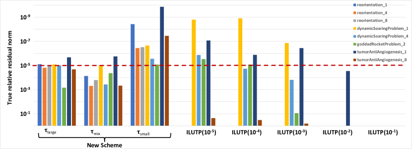
Figure 1: Final true relative residual norms of the new scheme and the baseline method for the symmetric case

Next, we consider the additional $M$-orthogonalization of the nullspace basis via the modified Gram-Schmidt procedure. The number of outer-inner iterations and the total number of nonzeros for the new scheme are presented in Tables 8, 9 and 10, respectively. In this case, the total number of nonzeros refers to the sum of the number of nonzeros of the nullspace basis, the $M$-orthogonalized nullspace basis and the nonzeros of the SPAI preconditioner (i.e., $nnz(\widetilde{Z})+nnz(\bar{Z})+nnz(\tilde{W})$). Although $\widetilde{Z}$ can be discarded after $\bar{Z}$ is computed, we include it in the sum as a measure of the peak memory requirement. When $\tau_{small}$ is used, there is not much difference in terms of inner and outer iterations, except for reorientation_8, where the number of average CG iterations drops from $20.5$ to $2.5$ if the nullspace basis is $M$-orthogonalized. When $\tau_{mix}$ is used, there are two problems for which the new scheme did not converge without $M$-orthogonalization, namely goddardRocketProblem_2 and tumorAntiAngiogenesis_8, these converge now with $M$-orthogonalization. GoddardRocketProblem_2, is particularly interesting, since it has a nullspace dimension of $1$, and hence $M$-orthogonalization is just normalizing the basis vector. The matrix $A$ has a condition number of $1.85\times 10^{15}$, i.e. it is almost singular, even though the condition number of the coefficient matrix $\mathcal{W}$ is $1.38\times 10^{7}$. In this case, the nullspace method becomes a more effective preconditioner with $M$-orthogonalization and the number of outer fGMRES iterations is reduced to $58$, without any increase in memory requirement. When $\tau_{large}$ is used, $M$-orthogonalization appears to cause more failures, because the nullspace basis is likely to be inaccurate to begin with, and further approximations only increase the error.

#	$\tau_{large}$	$\tau_{mix}$	$\tau_{small}$
1	19	$\ddagger$	2
2	$\ddagger$	$\ddagger$	$\S$
3	$\ddagger$	$\ddagger$	2
4	12	20	2
5	570	$\ddagger$	4
6	$\ddagger$	58	12
7	3	6	2
8	$\ddagger$	1	1

Table 8: Number of outer fGMRES iterations for the new scheme (symmetric case) with $M$-orthogonalization

#	$\tau_{large}$		$\tau_{mix}$		$\tau_{small}$
	cg	lsqr	cg	lsqr	cg	lsqr
1	2.0	235.9	2	641.8	1.0	866.5
2	2.0	157.3	1.9	980.6	$\S$	$\S$
3	2.4	153.0	1.9	958.3	2.5	766.3
4	2.0	87.1	2.0	354.0	1.0	599.5
5	2.0	285.5	3.0	848.9	1.8	$\ddagger$
6	1.0	68.5	1.0	511.8	1.0	$\ddagger$
7	2.0	136.0	2.0	141.2	1.0	144.8
8	8.0	128.6	4.0	721.0	6.0	763.0

Table 9: Average number of inner CG and LSQR iterations for the new scheme (symmetric case) with $M$-orthogonalization

#	$\tau_{large}$	$\tau_{mix}$	$\tau_{small}$
1	36,413	1,642	73,858
2	142,321	1,590	$\S$
3	162,901	2,061	1,272,471
4	45,250	27,759	50,769
5	881,668	94,735	1,218,169
6	183	87	185
7	4,681	2,276	8,145
8	6,045	1,952	24,301

Table 10: Number of nonzeros of the new scheme (symmetric case) with $M$-orthogonalization

6.2 Generalized case

As before, let us first consider the new scheme without $M$-orthogonalization. For the problems given in Table 2, in Table 11 we present the number of outer GMRES(10) and fGMRES(10) iterations for the baseline method and the new scheme, respectively. Here, ILUTP frequently fails, as it encounters a zero pivot, sometimes even when a stringent or a relaxed drop tolerance is used but converges for some arbitrary values of drop tolerances for the lid-driven cavity problem. In a number of cases, ILUTP fails because the final true relative residual norm is larger than the stopping tolerance. The new method converges for all problems without any failure, showing the robustness of the new scheme for the generalized problem set.

	New Scheme			ILUTP($\tau$)
#	$\tau_{large}$	$\tau_{mix}$	$\tau_{small}$	$10^{-5}$	$10^{-4}$	$10^{-3}$	$10^{-2}$	$10^{-1}$
1	3	2	2	3	$\dagger$	$\dagger$	$\dagger$	$\dagger$
2	2	2	2	2	$\dagger$	$\dagger$	$\dagger$	$\dagger$
3	2	1	1	2	4	6	12	13
4	2	2	2	$1^{\star}$	$2^{\star}$	3	6	$32^{\star}$
5	2	3	2	$1^{\star}$	$1^{\star}$	3	7	$44^{\star}$
6	3	3	1	$\dagger$	2	3	7	$\ddagger$
7	3	3	2	$\dagger$	$\dagger$	$\ddagger$	$9^{\star}$	$\ddagger$
8	4	3	2	$\dagger$	$\dagger$	$\ddagger$	10	$\dagger$

Table 11: Number of outer fGMRES/GMRES iterations for the generalized case

In Table 12, we report the total number of nonzeros for the new scheme (i.e., $nnz(\widetilde{Z})+nnz(\widetilde{W})$) and ILUTP($\tau$) (i.e., $nnz(L)+nnz(U)$). The best method among those that converge without any failure for each problem is given in bold. The new scheme achieves fewer nonzeros compared to ILUTP for 3 cases, while ILUTP is better than the new scheme for 5 cases. However, in most cases, the difference in the number of nonzeros is not significant.

	New Scheme			ILUTP($\tau$)
#	$\tau_{large}$	$\tau_{mix}$	$\tau_{small}$	$10^{-5}$	$10^{-4}$	$10^{-3}$	$10^{-2}$	$10^{-1}$
1	23,856	23,856	203,761	245,975	$\dagger$	$\dagger$	$\dagger$	$\dagger$
2	1,329	1,329	2,326	6,187	$\dagger$	$\dagger$	$\dagger$	$\dagger$
3	10,946	10,946	26,596	14,644	11,526	8,521	4,905	4,417
4	55,661	51,984	69,923	70,392⋆	66,804⋆	58,686	41,156	16,444⋆
5	55,591	55,584	69,946	$72,739^{\star}$	68,323⋆	60,242	46,078	19,095⋆
6	58,271	58,266	70,325	$\dagger$	67,989	60,271	45,570	20,011‡
7	60,019	60,042	70,842	$\dagger$	$\dagger$	64,229‡	46,681⋆	$\dagger$
8	63,143	63,118	71,699	$\dagger$	$\dagger$	62,842‡	45,280	$\dagger$

Table 12: Number of nonzeros of the preconditioners for the generalized case

In Table 13, we present the average number of inner fGMRES(10), LSQR and MRS iterations for the new scheme. While all are reasonably small for the circuit simulation systems, the number of inner fGMRES(10) and MRS iterations grow as the Reynold’s number increases for the lid-driven cavity problem. However, this growth is suppressed if $\tau_{large}$ is used. For generalized test problems, the number of LSQR iterations remained reasonably small for all problems, even without using any preconditioner. Figure 2 shows the final true relative residual norms of the new scheme and the baseline for the generalized case. The horizontal dashed line visualizes the stopping tolerance where the norm of the relative residual is equal to $10^{-5}$.

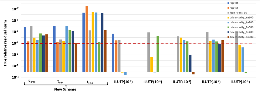
Figure 2: Final true relative residual norms of the new scheme and the baseline for the generalized case

#	$\tau_{large}$			$\tau_{mix}$			$\tau_{small}$
	fgmres	lsqr	mrs	fgmres	lsqr	mrs	fgmres	lsqr	mrs
1	3.0	1.5	2.9	4.0	1.5	4.0	2.0	1.5	4.0
2	2.0	1.0	5.0	2.0	1.0	7.0	2.0	1.0	7.0
3	3.0	1.0	2.0	4.0	1.0	3.3	2.0	1.0	3.5
4	2.5	16.8	17.8	3.0	24.3	27.5	2.0	25.3	27.5
5	2.0	16.5	31.8	3.0	23.7	48.0	2.0	24.8	47.8
6	3.7	17.3	101.4	5.0	23.3	164.5	3.0	23.5	151.7
7	9.0	17.5	230.3	10.0	23.8	374.0	7.0	23.8	360.7
8	52.5	18.3	493.9	81.3	22.8	791.9	132.5	27.8	809.6

Table 13: Average number of inner fGMRES, LSQR and MRS iterations for the new scheme (generalized case)

Next, we consider the additional $M$-orthogonalization of the nullspace basis via the modified Gram-Schmidt procedure. The number of outer fGMRES(10) iterations and the total number of nonzeros for the new scheme are given in Tables 14 and 15, respectively. As before, the total number of nonzeros refers to the sum of the number of nonzeros of the nullspace basis, the $M$-orthogonalized nullspace basis and the nonzeros of the SPAI preconditioner (i.e. $nnz(\widetilde{Z})+nnz(\bar{Z})+nnz(\tilde{W})$). The average number of inner fGMRES(10), LSQR, and MRS are given in Table 16. For test problems in the generalized case, we do not observe any significant differences when $M$-orthogonalization is performed. There is some increase in the number of nonzeros in most cases.

#	$\tau_{large}$	$\tau_{mix}$	$\tau_{small}$
1	2	2	1
2	2	2	2
3	2	1	1
4	3	4	2
5	3	4	2
6	3	3	2
7	3	5	2
8	4	5	2

Table 14: Number of outer fGMRES iterations for the new scheme (generalized case) with $M$-orthogonalization

#	$\tau_{large}$	$\tau_{mix}$	$\tau_{small}$
1	25,850	25,640	194,360
2	1,510	1,458	2,522
3	12,408	12,452	27,714
4	62,499	61,007	94,424
5	62,508	60,989	94,444
6	64,497	63,109	95,064
7	65,518	66,266	95,916
8	70,609	77,180	98,515

Table 15: Number of nonzeros of the new scheme for the new scheme (generalized case) with $M$-orthogonalization

#	$\tau_{large}$			$\tau_{mix}$			$\tau_{small}$
	fgmres	lsqr	mrs	fgmres	lsqr	mrs	fgmres	lsqr	mrs
1	3.0	1.5	2.8	3.5	1.5	4.0	2.0	1.5	4.0
2	2.0	1.0	5.0	2.0	1.0	7.0	1.5	1.0	7.0
3	2.5	1.0	2.0	3.0	1.0	3.3	2.0	1.0	3.0
4	2.0	19.8	18.5	3.0	22.1	27.8	2.0	29.5	27.5
5	2.3	20.0	32.0	3.0	21.8	48.4	2.0	29.0	48.5
6	3.0	18.2	100.1	4.8	21.6	164.8	3.0	29.0	151.7
7	8.0	19.2	216.0	54.8	21.4	567.2	7.0	29.3	358.4
8	54.5	17.9	460.9	72.0	21.4	752.2	124.5	28.0	810.6

Table 16: Average number of inner fGMRES, LSQR and MRS iterations for the new scheme (generalized case) with $M$-orthogonalization

6.3 General case

Finally, for the general problems given in Table 3, we present in Table 17 the number of outer GMRES(10) and fGMRES(10) iterations for the baseline method and the new scheme, respectively. The new scheme converges for all cases where $\tau_{mix}$ and $\tau_{small}$ are used, while ILUTP has at least one failure due to the encounter of a zero pivot for all drop tolerances. The new scheme fails in one case when $\tau_{large}$ is used due to reaching the maximum allowed iterations without reaching the required relative residual norm.

	New Scheme			ILUTP($\tau$)
#	$\tau_{large}$	$\tau_{mix}$	$\tau_{small}$	$10^{-5}$	$10^{-4}$	$10^{-3}$	$10^{-2}$	$10^{-1}$
1	3	3	2	3	5	$\dagger$	$\dagger$	$\dagger$
2	10	9	2	4	9	$\dagger$	$\dagger$	$\dagger$
3	2	2	1	1	2	2	3	4
4	7	2	1	1	2	2	3	4
5	34	5	4	1	2	2	3	4
6	27	11	11	1	2	2	3	4
7	4	17	1	2	2	4	10	$\dagger$
8	$\ddagger$	53	5	$\dagger$	$\dagger$	$\dagger$	$\dagger$	$\dagger$
9	9	2	2	1	1	$\dagger$	$\dagger$	$\dagger$

Table 17: Number of outer fGMRES/GMRES iterations for the general case

In Table 18, we report the total number of nonzeros for the new scheme (i.e., $nnz(\widetilde{Z})+nnz(\widetilde{U})+nnz(\widetilde{W})$) and ILUTP($\tau$) (i.e., $nnz(L)+nnz(U)$). The best method among those that converge without any failure for each problem is given in bold. The new scheme not only converges without any failures for all problems but also achieves fewer nonzeros compared to ILUTP for all cases, except for two (garon_1 and garon_2). We note that for these two cases, even though ILUTP achieves fewer number of nonzeros, it is likely to fail if the drop tolerance is not chosen correctly.

	New Scheme			ILUTP($\tau$)
#	$\tau_{large}$	$\tau_{mix}$	$\tau_{small}$	$10^{-5}$	$10^{-4}$	$10^{-3}$	$10^{-2}$	$10^{-1}$
1	1,252,275	1,252,275	2,204,857	644,190	623,798	$\dagger$	$\dagger$	$\dagger$
2	18,037,895	18,037,895	31,745,441	5,502,974	5,345,750	$\dagger$	$\dagger$	$\dagger$
3	162	162	162	1,829	1,797	1,642	1,229	640
4	612	612	612	2,529	2,497	2,342	1,860	1,205
5	1,962	1,962	1,962	4,629	4,597	4,442	3,618	2,882
6	7,200	7,200	7,200	12,777	12,745	11,603	10,233	9,344
7	1,885	1,688	1,875	28,035	27,955	27,527	25,366	$\dagger$
8	$114\ddagger$	90	134	$\dagger$	$\dagger$	$\dagger$	$\dagger$	$\dagger$
9	320	320	320	5,298	5,298	$\dagger$	$\dagger$	$\dagger$

Table 18: Number of nonzeros of the preconditioners for the general case

In Table 19, we present the average number of inner fGMRES(10), LSQR and MRS iterations for the new scheme. For all problems (except garon_1 and garon_2) the average number of inner fGMRES(10) iterations is small, even if $\tau_{large}$ and $\tau_{mix}$ are used. As in the other problem classes, the average number of LSQR iterations can be quite large for the set of general problems as well. The average number of MRS iterations is reasonably small for all $\tau_{\{large,mix,small\}}$.

#	$\tau_{large}$			$\tau_{mix}$			$\tau_{small}$
	fgmres	lsqr	mrs	fgmres	lsqr	mrs	fgmres	lsqr	mrs
1	671.0	67.3	6.3	753.3	86.8	7.0	6.0	107.3	7.0
2	987.0	113.1	1.3	$\ddagger$	152.1	1.9	4.0	197.0	1.9
3	1.0	11.3	1.0	1.0	11.8	1.0	1.0	12.0	1.0
4	1.0	45.4	1.0	1.0	92.3	1.0	1.0	94.5	1.0
5	1.0	130.1	1.0	1.0	392.0	1.0	1.0	500.5	1.0
6	1.0	216.5	1.0	1.0	500.5	1.0	1.0	500.5	1.0
7	8.0	87.1	8.0	7.0	95.4	10.6	7.0	88.0	9.7
8	7.3	70.1	7.3	7.0	155.7	7.5	6.2	373.9	8.3
9	2.0	178.6	7.4	2.0	527.0	1.0	2.0	611.0	1.0

Table 19: Average number of inner fGMRES, LSQR and MRS iterations for the new scheme (general case)

Figure 3 shows the final true relative residual norms of the new scheme and the baseline method for the general case. The horizontal dashed line visualizes the stopping tolerance where the norm of the relative residual is equal to $10^{-5}$.

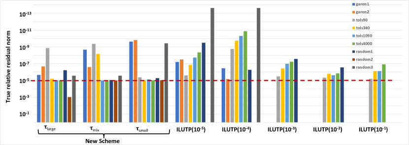
Figure 3: Final true relative residual norms of the new scheme and the baseline for the generalized case

7 Conclusions

We have introduced a new class of multilayer iterative schemes for solving sparse linear systems in saddle point structure. We have presented a theoretical analysis for the (approximate) nullspace method. We have demonstrated the effectiveness of the new schemes by solving linear systems that arise in a variety of applications and compare them to a classical preconditioned iterative scheme. The new schemes may benefit from further preconditioning in the Krylov subspace methods for solving over/underdetermined linear least squares problems. This is currently under investigation. Although rarely encountered in practice, we believe that a further generalization of the new schemes for linear systems where the $(2,2)$-block is non-square, as well as generalizing the new schemes for over/underdetermined linear least squares problems with saddle point structures is possible. Furthermore, a parallel implementation of the new schemes for large-scale problems is also planned as a future work.

References

- [1] F. Achleitner, A. Arnold, and V. Mehrmann. Hypocoercivity and controllability in linear semi-dissipative ODEs and DAEs. ZAMM Z. Angew. Math. Mech., 103(7):e202100171, 2023. http://arxiv.org/abs/2104.07619.
- [2] M. Benzi, J. K. Cullum, and M. Tuma. Robust approximate inverse preconditioning for the conjugate gradient method. SIAM J. Sci. Comput., 22(4):1318–1332, 2000.
- [3] M. Benzi, G. H. Golub, and J. Liesen. Numerical solution of saddle point problems. Acta Numerica, 14:1–137, 2005.
- [4] M. Benzi and C. D. Meyer. A direct projection method for sparse linear systems. SIAM J. Sci. Comput., 16(5):1159–1176, 1995.
- [5] M. Benzi, D. B. Szyld, and A. Van Duin. Orderings for incomplete factorization preconditioning of nonsymmetric problems. SIAM J. Sci. Comput., 20(5):1652–1670, 1999.
- [6] J. T. Betts. Practical Methods for Optimal Control and Estimation Using Nonlinear Programming, volume 19. SIAM Publications, Philadelphia, PA, 2010.
- [7] F. Brezzi. On the existence, uniqueness and approximation of saddle-point problems arising from Lagrangian multipliers. Public. Séminaires de Math. Inform. de Rennes, (S4):1–26, 1974.
- [8] M. T. Chu, R. E. Funderlic, and G. H. Golub. A rank–one reduction formula and its applications to matrix factorizations. SIAM Review, 37(4):512–530, 1995.
- [9] T. A. Davis and Y. Hu. The University of Florida sparse matrix collection. ACM Trans. Math. Software (TOMS), 38(1):1–25, 2011.
- [10] H. C. Elman, A. Ramage, and D. J. Silvester. IFISS: A computational laboratory for investigating incompressible flow problems. SIAM Review, 56(2):261–273, 2014.
- [11] P. E. Gill, W. Murray, and M. H. Wright. Numerical Linear Algebra and Optimization. SIAM Publications, Philadelphia, PA, 2021.
- [12] R. H. Goddard. A method of reaching extreme altitudes. Nature, 105:809–811, 1920.
- [13] G. H. Golub and C. F. Van Loan. Matrix Computations. Johns Hopkins Studies in the Mathematical Sciences. Johns Hopkins University Press, Baltimore, MD, third edition, 1996.
- [14] G. H. Golub and A. J. Wathen. An iteration for indefinite systems and its application to the Navier–Stokes equations. SIAM J. Sci. Comput., 19(2):530–539, 1998.
- [15] C. Greif, S. He, and P. Liu. SYM-ILDL: Incomplete LDLT factorization of symmetric indefinite and skew-symmetric matrices. ACM Trans. Math. Software (TOMS), 44(1):1–21, 2017.
- [16] C. Güdücü, J. Liesen, V. Mehrmann, and D. Szyld. On non-Hermitian positive (semi)definite linear algebraic systems arising from dissipative Hamiltonian DAEs. SIAM J. Sci. Comput., 44:A2871–A2894, 2022.
- [17] M. R. Hestenes, E. Stiefel, et al. Methods of conjugate gradients for solving linear systems. J. Research National Bureau of Standards, 49(6):409–436, 1952.
- [18] R. Idema and C. Vuik. A minimal residual method for shifted skew-symmetric systems. Delft University of Technology, 2007.
- [19] R. Idema and C. Vuik. A comparison of Krylov methods for shifted skew-symmetric systems. arXiv preprint 2304.04092, 2023.
- [20] E. Jiang. Algorithm for solving shifted skew-symmetric linear system. Front. Math. China, 2(2):227–242, 2007.
- [21] U. Ledzewicz and H. Schättler. Analysis of optimal controls for a mathematical model of tumour anti-angiogenesis. Optimal Contr. Appl. Methods, 29(1):41–57, 2008.
- [22] M. Manguoğlu and V. Mehrmann. A two-level iterative scheme for general sparse linear systems based on approximate skew-symmetrizers. Electron. Trans. Numer. Anal., 54:370–391, 2021.
- [23] V. Mehrmann and R. Morandin. Structure-preserving discretization for port-hamiltonian descriptor systems. In 58th IEEE Conference on Decision and Control (CDC), 9.-12.12.19, Nice, pages 6863–6868. IEEE, 2019.
- [24] C. C. Paige and M. A. Saunders. LSQR: An algorithm for sparse linear equations and sparse least squares. ACM Trans. Math. Software (TOMS), 8(1):43–71, 1982.
- [25] D. Rapoport. A Nonlinear Lanczos Algorithm and the Stationary Navier-Stokes Equation. PhD thesis, Department of Mathematics, Courant Institute, New York University, 1978.
- [26] M. Rozložník. Saddle-point problems and their iterative solution. Springer Verlag, Heidelberg, Germany, 2018.
- [27] Y. Saad. A flexible inner-outer preconditioned GMRES algorithm. SIAM J. Sci. Comput., 14(2):461–469, 1993.
- [28] Y. Saad. A flexible inner-outer preconditioned GMRES algorithm. SIAM J. Sci. Comput., 14(2):461–469, 1993.
- [29] J. Schöberl and W. Zulehner. Symmetric indefinite preconditioners for saddle point problems with applications to pde-constrained optimization problems. SIAM J. Matrix Anal. Appl., 29(3):752–773, 2007.
- [30] J. Scott and M. Tuma. A null-space approach for large-scale symmetric saddle point systems with a small and non zero (2, 2) block. Numerical Algorithms, 90(4):1639–1667, 2022.
- [31] A. J. Wathen. Preconditioning. Acta Numerica, 24:329–376, 2015.
- [32] O. Widlund. A Lanczos method for a class of nonsymmetric systems of linear equations. SIAM J. Numer. Anal., 15(4):801–812, 1978.
- [33] Y. J. Zhao. Optimal patterns of glider dynamic soaring. Optimal Contr. Appl. Methods, 25(2):67–89, 2004.