Low mode approximation in the axion magnetohydrodynamics

Abstract

We study the evolution of interacting large scale magnetic and axionic fields. Based on the new induction equation accounting for the contribution of spatially inhomogeneous axions, we consider the evolution of a magnetized spherical axion structure. Using the thin layer approximation, we derive the system of the nonlinear ordinary differential equations for harmonics of poloidal and toroidal magnetic fields, as well as for the axion field. In this system, we account for up to four modes. Considering this small and dense axion clump to be in a solar plasma, we numerically simulate the evolution of magnetic fields. We obtain that the behavior of magnetic fields depends on the initial fields configuration. Moreover, we find an indication on a magnetic field instability in the magnetohydrodynamics with inhomogeneous axions.

1 Introduction

Nowadays it is commonly accepted that a significant fraction of the universe mass is present in the form of dark matter, which reveals itself mainly by the gravitational interaction. Despite multiple candidates for dark matter particles were proposed, the nature of dark matter is still unclear. The most plausible candidates for dark matter constituents are light particles called axions [1], which were first proposed in the quantum chromodynamics (QCD) [2, 3, 4]. The masses of QCD axions are in the range $10^{-6}\,\text{eV}<m<10^{-4}\,\text{eV}$. However, much lighter axion like particles (ALPs) with masses $m<10^{-11}\,\text{eV}$ are also considered [5, 6]. In spite of numerous attempts aimed to the direct detection of axions and ALPs in a laboratory [7, 8], these particles are still elusive.

Despite dark matter interacts mainly gravitationally, axions and ALPs are admitted to interact with electromagnetic fields, although the corresponding coupling constant is quite small. The interaction between dark and usual matter results in various interesting phenomena like the emission of ultra-high-energy cosmic rays [9] and various multi-messenger effects [10]. Moreover, gamma ray bursts with certain energies are explained in Ref. [11] by decays of ALPs.

Axions background proceeding from the early universe is likely to be spatially homogeneous. However, if the Peccei–Quinn (PQ) phase transition happens after the reheating during the inflation, inhomogeneities of axions can be present. They can result in the formation of axion miniclusters [12, 13] and axion stars [14, 15].

The electrodynamics equations in presence of axions were obtained in Refs. [16, 17] to describe possible experiments to detect these particles. The interaction of magnetic fields with spatially homogeneous axions were shown in Ref. [18] to cause the magnetic field instability. We considered the magnetohydrodynamics (MHD) in the presence of spatially homogeneous [19] and inhomogeneous [20] axions in the early universe. Besides the magnetic field instability the parametric instability is reported in Ref. [21] to take place in the axion electrodynamics.

Recently, in Refs. [22, 23], we derived the new induction equation for the magnetic field evolution in presence of inhomogeneous axions and applied it for magnetic fields with various configurations including quite nontrivial ones related to the Hopf fibration. This new equation was used in Ref. [24] to study the magnetic field behavior in a dense axion star in solar plasma. A possible implication of the obtained results to the solar corona heating was discussed in Ref. [24]. The axion dynamo in a neutron star was considered in Ref. [25]. In the present paper, we develop the research initiated in Ref. [24].

This work is organized in the following way. First, in Sec. 2, starting with the new induction equation accounting for the axions inhomogeneity, we derive the main equations describing mutual evolution of axion and magnetic fields. Then, we formulate the initial condition and fix the rest of the parameters of the system. In Sec. 3, we present the results of numerical simulations of the magnetic fields evolution inside a spherical axionic clump in solar plasma. Finally, we conclude in Sec. 4. The ordinary differential equations for the harmonics of axion and magnetic fields are derived in Appendix A.

2 MHD in presence of axions

The new induction equation, accounting for the time dependent and spatially inhomogeneous axion field $\varphi(t,\mathbf{x})$, has the form [22, 23],

$$\frac{\partial\mathbf{B}}{\partial t}=\nabla\times\left[\mathbf{b}\times(\nabla\times\mathbf{B})+\alpha\mathbf{B}-\eta(\nabla\times\mathbf{B})\right],$$ (2.1)

where $\alpha=g_{a\gamma}\eta\partial_{t}\varphi$ is the $\alpha$-dynamo parameter, which is nonzero for the time dependent $\varphi$, $\mathbf{b}=g_{a\gamma}\eta^{2}\nabla\varphi$ is the axial vector being nonzero in case of the spatial inhomogeneous $\varphi$, $\eta$ is the magnetic diffusion coefficient, and $g_{a\gamma}$ is the axion-to-photon coupling constant. We should add to Eq. (2.1) the equation for the axions evolution in presence of a magnetic field. It is the inhomogeneous Klein-Gordon equation,

$$\frac{\partial^{2}\varphi}{\partial t^{2}}-\Delta\varphi+m^{2}\varphi=\eta g_{a\gamma}\mathbf{B}\cdot(\nabla\times\mathbf{B}),$$ (2.2)

where $m$ is the axion mass. Note that, in Eqs. (2.1) and (2.2), we keep only the terms linear in $g_{a\gamma}$.

We use the spherical coordinates $(r,\vartheta,\phi)$ to describe the evolution of $\mathbf{B}$ and $\varphi$ in Eqs. (2.1) and (2.2). The magnetic field is taken to have the poloidal $\mathbf{B}_{p}=\nabla\times(A\mathbf{e}_{\phi})$ and toroidal $\mathbf{B}_{t}=B\mathbf{e}_{\phi}$ components, $\mathbf{B}=\mathbf{B}_{p}+\mathbf{B}_{t}$, where $A$ and $B$ are the new functions of time and coordinates and $\mathbf{e}_{\phi}$ is the unit vector along the $\phi$ variation. We suppose that $A$, $B$, and $\varphi$ are axially symmetric and have the following properties in reflection with respect to the equatorial plane:

$$A(r,\pi-\vartheta,t)=A(r,\vartheta,t),\quad B(r,\pi-\vartheta,t)=-B(r,\vartheta,t),\quad\varphi(r,\pi-\vartheta,t)=-\varphi(r,\vartheta,t),$$ (2.3)

since $A\mathbf{e}_{\phi}$ is the vector, $\mathbf{B}_{t}$ is the axial vector, and $\varphi$ is the pseudoscalar.

Following Ref. [26], we assume that the functions $A$, $B$, and $\varphi$ evolve in a thin layer $R<r<R+\mathrm{d}r$, where $R$ is the typical radius of the axion structure and $\mathrm{d}r\ll R$ is the layer width. In this approximation, we can neglect the radial dependence in Eqs. (2.1) and (2.2), where we set $r=R$ and $\partial_{r}=0$. Note that we keep the dependence on the latitude $\vartheta$. The next reasonable approximation is based on the decomposition over the angular harmonics and keeping only a few of them. It is called the low mode approximation [27].

Using the dimensionless variables

$$\mathcal{A}=g_{a\gamma}A,\quad\mathcal{B}=g_{a\gamma}RB,\quad\Phi=\frac{g_{a\gamma}\eta}{R}\varphi,\quad\tau=\frac{\eta t}{R^{2}},$$ (2.4)

we take that

$$\mathcal{A}(\vartheta,\tau)=\sum_{k=1}^{4}a_{k}(\tau)\sin(2k+1)\vartheta,\quad\mathcal{B}(\vartheta,\tau)=\sum_{k=1}^{4}b_{k}(\tau)\sin 2k\vartheta,\quad\Phi(\vartheta,\tau)=\sum_{k=1}^{4}\phi_{k}(\tau)\sin 2k\vartheta.$$ (2.5)

The decomposition in Eq. (2.5) accounts for the symmetry properties in Eq. (2.3). Unlike Ref. [24], where only two harmonics were taken into account, we deal with four harmonics in Eq. (2.5). As found in Ref. [28], in treating solar magnetic fields in frames of the $\alpha\Omega$-dynamo, one has to account for up to five harmonics.

Based on the decomposition in Eq. (2.5) and using the technique in Ref. [24], we obtain the system of nonlinear ordinary differential equations for the coefficients $a_{k}$, $b_{k}$, and $\phi_{k}$. Since this system is quite cumbersome, we present it in Eq. (A) in Appendix A. In Eq. (A), $\mu=mR^{2}/\eta$ and $\kappa=R/\eta$ are is the dimensionless axion mass and wave vector respectively.

The system in Eq. (A) is to be solved numerically. For this purpose we have to specify the initial condition for the functions $a_{k}$, $b_{k}$, and $\phi_{k}$. To highlight the influence of the greater number of harmonics on the evolution of magnetic fields we choose the parameters of the system and the initial condition in the same form as in Ref. [24]. Analogously to Ref. [24], we suppose that an axionic structure exists in the solar plasma.

First, we set the parameters of axions. The axion mass is taken to be $m=10^{-5}\,\text{eV}$, i.e. we consider a QCD axion. The size of the axion clump is $R=0.7\,\text{cm}$. The initial energy density of axions inside such a small axion star is $\rho_{0}\approx 10^{-2}m^{2}f_{a}^{2}$, where $f_{a}\approx 5.7\times 10^{11}\,\text{GeV}$ is the PQ constant for the chosen axion mass. Here, we utilize the approximate relation between the axion mass and the PQ constant, $\tfrac{f_{a}}{10^{12}\,\text{GeV}}\approx 5.7\left(\tfrac{m}{10^{-6}\,\text{eV}}\right)^{-1}$ (see, e.g., Ref. [29]). Thus, the axion-to-photon coupling constant, used in Eq. (2.4), is also uniquely defined by the axion mass, $g_{a\gamma}=\tfrac{\alpha_{\mathrm{em}}}{2\pi f_{a}}=2\times 10^{-15}\,\text{GeV}^{-1}$, where $\alpha_{\mathrm{em}}=7.3\times 10^{-3}$ is the fine structure constant.

The size and the energy density of the axion clump, used in our simulations, indicate that we deal with a dense axion star. The existence of such an object was proposed in Ref. [30], where it was claimed to be stable. However, the analysis in Ref. [31] showed that dense axion stars decay in a short time interval. The instability of dense stars is because axions in these objects do not have a conserved quantum number. This case is opposite to dilute stars where the quantity $\smallint\mathrm{d}^{3}x\varphi^{\dagger}\varphi$ is conserved (see, e.g., Ref. [32]).

It was reported in Ref. [31] that, in some cases, the lifetime of a dense star can reach $\tau_{\mathrm{life}}\gtrsim 10^{-8}\text{s}$ for $m=10^{-5}\,\text{eV}$. We shall see shortly in Sec. 3 that typical frequencies of magnetic fields oscillations are $f_{\mathrm{B}}\sim 10^{11}\,\text{Hz}$. Therefore, the period of magnetic oscillations is $\tau_{\mathrm{B}}=f_{\mathrm{B}}^{-1}\ll\tau_{\mathrm{life}}$. It means that magnetic fields oscillations can happen multiple times within the star lifetime. Hence, although a dense axion star is quasi-stable, it provides a reasonable initial condition for the studies of oscillating magnetic fields driven by axions.

We take the magnetic diffusion coefficient as $\eta=10^{10}\,\text{cm}^{2}\cdot\text{s}^{-1}$, which is close to the observed value and corresponds to the turbulent magnetic diffusion [33]. In this case, using the chosen axions energy density in the star, one has that $\phi_{1}(0)=2\times 10^{-5}$, $\phi_{2,\dots,4}(0)=0$, and $\dot{\phi}_{1,\dots,4}(0)=0$.

We suppose that the seed magnetic field is $B(0)=1\,\text{G}$, which corresponds to the strength in the quiet Sun. We study the situations of both poloidal and toroidal seed fields. In the former case, $a_{1}(0)=1.4\times 10^{-21}$, $a_{2,\dots,4}(0)=0$, and $b_{1,\dots,4}(0)=0$ for the chosen parameters of the system. In the latter case, one has that $b_{1}(0)=1.4\times 10^{-21}$, $b_{2,\dots,4}(0)=0$, and $a_{1,\dots,4}(0)=0$. More detailed justification of the choice of the initial initial condition and the parameters of an axion is present in Ref. [24].

3 Results

In this section, we present the results of the numerical solution of Eq. (A) for the initial condition specified in Sec. 2. In Figs. 1, 1, 2, and 2, one can see the time evolution of the harmonics of poloidal $a_{i}$ and toroidal $b_{i}$ fields for the cases of either poloidal or toroidal seed fields. It can be seen in Figs. 1 and 2 that oscillations of the toroidal harmonics are excited in both cases. However, the oscillating poloidal field exists only when one has a seed poloidal field; cf. Figs. 1 and 2. It is the new feature compared to Ref. [24]. The insets in Figs. 1, 1, 2, and 2 demonstrate that the initial condition is satisfied for $a_{i}$ and $b_{i}$.

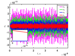
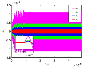
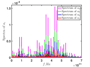
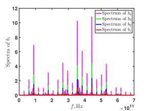
Figure 1: Evolution of the magnetic fields harmonics in a dense axion star when a seed poloidal field is present. The parameters of the system are the following: the axion mass is $m=10^{-5}\,\text{eV}$, the axion clump radius is $R=0.7\,\text{cm}$, the seed poloidal magnetic field is $B_{\mathrm{pol}}(0)=1\,\text{G}$, whereas $B_{\mathrm{tor}}(0)=0$. (a) The time evolution of the poloidal harmonics. (b) The behavior of toroidal harmonics. (c) The spectra of poloidal harmonics. (d) The spectra of toroidal harmonics. The insets in panels (a) and (b) show the evolution of harmonics on short time intervals.

Moreover, the next interesting feature to be noticed in Figs. 1, 1, and 2 is that the amplitudes of oscillations increases for higher harmonics. It can be the indication that magnetic field is generically unstable in presence of oscillating inhomogeneous axions. This feature can be also observed in Figs. 1, 1, and 2 where the spectra of harmonics are shown. Note that we do not discuss the spectra of $a_{i}$ in Fig. 2 which are mostly continuous since oscillations of poloidal harmonics are not excited. We also mention in Figs. 1, 1, and 2 that typical oscillations frequencies are higher than those in the two harmonics case considered in Ref. [24].

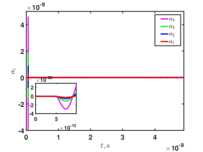
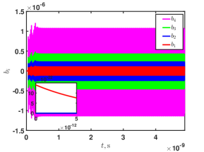
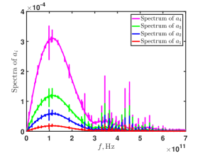
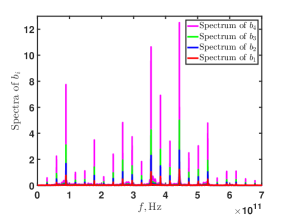
Figure 2: The same as in Fig. 1 for a seed toroidal field, $B_{\mathrm{tor}}(0)=1\,\text{G}$ and $B_{\mathrm{pol}}(0)=0$.

Finally, in Fig. 3, we depict the time evolution of the axion field harmonics $\phi_{i}$ for both poloidal and toroidal seed magnetic fields. First, one can see that the evolution of axions is almost unaffected by the magnetic field; cf. Figs. 3 and 3. This feature was mentioned in Refs. [22, 23]. Second, the amplitudes of oscillating harmonics decrease for the higher harmonics numbers. It means that oscillations of axions are likely to be stable. Of course, the stability of axions oscillations is valid while $t\ll\tau_{\mathrm{life}}$.

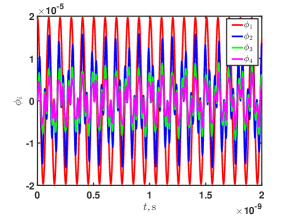
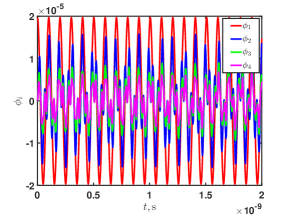
Figure 3: The evolution of the axion field harmonics for (a) the seed poloidal magnetic field and (b) the seed toroidal field. The parameters of the system and the initial condition correspond to Figs. 1 and 2.

4 Conclusion

In the present work, we have studied the evolution of magnetic fields driven by time dependent and spatially inhomogeneous axion fields. Based on the recently derived induction equation which accounts for the axions contribution, we have considered a magnetized axion clump embedded in solar plasma. The mutual evolution of axions and magnetic fields has been examined in a thin layer within the low mode approximation. It allowed us to derive the system of nonlinear ordinary differential equations for the amplitudes of the harmonics. This system has been solved numerically in the case of a dense axion star, having a small radius, surrounded by solar plasma with realistic characteristics.

Contrary to Ref. [24], where only two harmonics were taken into account, now we have considered up to four modes in Eq. (2.5). The extension of the decomposition over the zonal harmonics is motivated by the result in Ref. [28] that higher harmonics can play a crucial role in dynamo problems.

The consideration of higher harmonics enabled us to reveal several interesting features in the axion MHD. First, we have noticed that different seed magnetic fields result in the different subsequent magnetic fields evolution. We have obtained that oscillations of both poloidal and toroidal fields are excited only for a seed poloidal field. Thus, such an initial magnetic fields configuration seems to be more stable. Indeed, as shown in Ref. [34] a long lived astrophysical magnetic field should have both poloidal and toroidal components.

Second, we have obtained that higher harmonics of the magnetic field have greater amplitudes. In some situations, this feature can be noticed in the two modes case considered in Ref. [24]. However, now this fact can be seen with a naked eye; cf. Figs. 1 and 2. It can be interpreted as the indication that a magnetic field instability is present in MHD with inhomogeneous axions. Revealing the source of such an instability is an interesting and important problem which requires a separate special attention.

We also mention that we have confirmed our previous result in Refs. [22, 23] that axions almost are not affected by the magnetic fields. Moreover the axion field harmonics with higher numbers have decreasing amplitudes contrary to magnetic ones. Thus, axions oscillations are likely to be quasi-stable.

We have considered a small axionic clump with a relatively high energy density. It corresponds to a dense axion star described in Ref. [30]. Such an axion star was shown in Ref. [31] to be quasi-stable. It decays after $\tau_{\mathrm{life}}\sim 10^{-8}\,\text{s}$ [31] because of the axions emission [32]. However, the time scale of magnetic fields oscillations, predicted in our work, is much shorter than $\tau_{\mathrm{life}}$. Thus, we may neglect the instability of a dense axion star while studying the excitation of magnetic fields oscillations.

In our work, we do not discuss the formation of dense magnetized axion stars. Taking into account their short lifetime, they cannot have a cosmological origin. Nonetheless, axions are reported in Ref. [35] to be able to concentrate around usual stars, like the Sun. The existence of quite exotic axionic objects, e.g., axion quark nuggets, in the Sun was suggested in Ref. [36]. Perhaps, dense magnetized axion stars can also arise in stellar interiors. However, this issue should be studied separately.

The results of the present work can have the implication to the problem of the solar corona heating as suggested in Ref. [24]. Previously, the involvement of dark matter to the solar corona heating and to the radio emission of the Sun was discussed in Refs. [36, 37].

Appendix A Ordinary differential equations for harmonics

The basis functions in Eq. (2.5) obey the orthogonality condition,

$$\frac{2}{\pi}\int_{0}^{\pi}\sin(n\vartheta)\sin(k\vartheta)\mathrm{d}\vartheta=\delta_{nk}.$$ (A.1)

Using Eq. (A.1), we can straightforwardly derive the following system of ordinary differential equations for the functions $a_{k}$, $b_{k}$, and $\phi_{k}$:

$$\dot{a}_{1}= -2(a_{1}+a_{2}+a_{3}+a_{4})+\frac{2}{\pi}\bigg{(}-\frac{16}{315}b_{1}\psi_{3}-\frac{64}{3465}b_{1}\psi_{4}-\frac{128}{2145}b_{2}\psi_{4}-\frac{16}{315}b_{3}\psi_{1}$$

$$-\frac{64}{3465}b_{4}\psi_{1}-\frac{128}{2145}b_{4}\psi_{2}-\frac{64}{15}b_{1}\phi_{1}-\frac{1024}{63}b_{2}\phi_{2}-\frac{5184}{143}b_{3}\phi_{3}-\frac{16384}{255}b_{4}\phi_{4}$$

$$+\frac{16}{15}b_{1}\psi_{1}+\frac{64}{63}b_{2}\psi_{2}+\frac{144}{143}b_{3}\psi_{3}+\frac{256}{255}b_{4}\psi_{4}-\frac{64}{195}b_{3}\psi_{4}-\frac{64}{195}b_{4}\psi_{3}-\frac{32}{99}b_{2}\psi_{3}$$

$$-\frac{32}{99}b_{3}\psi_{2}+\frac{4096}{195}b_{3}\phi_{4}+\frac{768}{65}b_{4}\phi_{3}-\frac{32}{105}b_{1}\psi_{2}-\frac{32}{105}b_{2}\psi_{1}+\frac{256}{3465}b_{4}\phi_{1}+\frac{128}{11}b_{2}\phi_{3}$$

$$+\frac{512}{99}b_{3}\phi_{2}+\frac{8192}{2145}b_{2}\phi_{4}+\frac{2048}{2145}b_{4}\phi_{2}+\frac{512}{105}b_{1}\phi_{2}+\frac{128}{105}b_{2}\phi_{1}+\frac{64}{35}b_{1}\phi_{3}+\frac{64}{315}b_{3}\phi_{1}$$

$$+\frac{4096}{3465}b_{1}\phi_{4}\bigg{)},$$

$$\dot{a}_{2}= -6(2a_{2}+a_{3}+a_{4})+\frac{2}{\pi}\bigg{(}-\frac{144}{385}b_{1}\psi_{3}-\frac{64}{819}b_{1}\psi_{4}-\frac{128}{315}b_{2}\psi_{4}-\frac{144}{385}b_{3}\psi_{1}$$

$$-\frac{64}{819}b_{4}\psi_{1}-\frac{128}{315}b_{4}\psi_{2}-\frac{64}{35}b_{1}\phi_{1}-\frac{20992}{3465}b_{2}\phi_{2}-\frac{27328}{2145}b_{3}\phi_{3}-\frac{1390592}{62985}b_{4}\phi_{4}$$

$$+\frac{16}{21}b_{1}\psi_{1}+\frac{64}{165}b_{2}\psi_{2}+\frac{16}{45}b_{3}\psi_{3}+\frac{256}{741}b_{4}\psi_{4}+\frac{576}{935}b_{3}\psi_{4}+\frac{576}{935}b_{4}\psi_{3}+\frac{288}{455}b_{2}\psi_{3}$$

$$+\frac{288}{455}b_{3}\psi_{2}-\frac{813568}{36465}b_{3}\phi_{4}-\frac{424704}{12155}b_{4}\phi_{3}+\frac{32}{45}b_{1}\psi_{2}+\frac{32}{45}b_{2}\psi_{1}+\frac{24832}{45045}b_{4}\phi_{1}$$

$$-\frac{148352}{15015}b_{2}\phi_{3}-\frac{837376}{45045}b_{3}\phi_{2}+\frac{318464}{15015}b_{2}\phi_{4}+\frac{80896}{9009}b_{4}\phi_{2}-\frac{256}{105}b_{1}\phi_{2}$$

$$-\frac{2176}{315}b_{2}\phi_{1}+\frac{11584}{1155}b_{1}\phi_{3}+\frac{9664}{3465}b_{3}\phi_{1}+\frac{65024}{15015}b_{1}\phi_{4}\bigg{)},$$

$$\dot{a}_{3}= -10(3a_{3}+a_{4})+\frac{2}{\pi}\bigg{(}\frac{80}{117}b_{1}\psi_{3}-\frac{64}{165}b_{1}\psi_{4}+\frac{640}{1071}b_{2}\psi_{4}+\frac{80}{117}b_{3}\psi_{1}-\frac{64}{165}b_{4}\psi_{1}$$

$$+\frac{640}{1071}b_{4}\psi_{2}-\frac{192}{35}b_{1}\phi_{1}-\frac{37376}{9009}b_{2}\phi_{2}-\frac{2135488}{255255}b_{3}\phi_{3}-\frac{13588480}{969969}b_{4}\phi_{4}-\frac{16}{45}b_{1}\psi_{1}$$

$$+\frac{64}{195}b_{2}\psi_{2}+\frac{144}{595}b_{3}\psi_{3}+\frac{256}{1155}b_{4}\psi_{4}+\frac{320}{1197}b_{3}\psi_{4}+\frac{320}{1197}b_{4}\psi_{3}+\frac{32}{105}b_{2}\psi_{3}+\frac{32}{105}b_{3}\psi_{2}$$

$$-\frac{138538496}{14549535}b_{3}\phi_{4}-\frac{72285952}{4849845}b_{4}\phi_{3}+\frac{160}{231}b_{1}\psi_{2}+\frac{160}{231}b_{2}\psi_{1}+\frac{18688}{4095}b_{4}\phi_{1}-\frac{14464}{3003}b_{2}\phi_{3}$$

$$-\frac{364288}{45045}b_{3}\phi_{2}-\frac{7773184}{765765}b_{2}\phi_{4}-\frac{17724416}{765765}b_{4}\phi_{2}-\frac{1280}{693}b_{1}\phi_{2}-\frac{896}{495}b_{2}\phi_{1}-\frac{320}{143}b_{1}\phi_{3}$$

$$-\frac{45504}{5005}b_{3}\phi_{1}+\frac{31232}{2145}b_{1}\phi_{4}\bigg{)},$$

$$\dot{a}_{4}= -56a_{4}+\frac{2}{\pi}\bigg{(}\frac{112}{165}b_{1}\psi_{3}+\frac{448}{663}b_{1}\psi_{4}+\frac{896}{3135}b_{2}\psi_{4}+\frac{112}{165}b_{3}\psi_{1}+\frac{448}{663}b_{4}\psi_{1}+\frac{896}{3135}b_{4}\psi_{2}$$

$$-\frac{9536}{3465}b_{1}\phi_{1}-\frac{34816}{45045}b_{2}\phi_{2}-\frac{4525504}{692835}b_{3}\phi_{3}-\frac{3595882496}{334639305}b_{4}\phi_{4}-\frac{16}{231}b_{1}\psi_{1}$$

$$+\frac{64}{105}b_{2}\psi_{2}+\frac{144}{665}b_{3}\psi_{3}+\frac{256}{1449}b_{4}\psi_{4}+\frac{64}{315}b_{3}\psi_{4}+\frac{64}{315}b_{4}\psi_{3}+\frac{224}{765}b_{2}\psi_{3}$$

$$+\frac{224}{765}b_{3}\psi_{2}-\frac{14990336}{2078505}b_{3}\phi_{4}-\frac{49881856}{4849845}b_{4}\phi_{3}-\frac{224}{585}b_{1}\psi_{2}-\frac{224}{585}b_{2}\psi_{1}-\frac{8440064}{765765}b_{4}\phi_{1}$$

$$-\frac{144256}{36465}b_{2}\phi_{3}-\frac{1319936}{255255}b_{3}\phi_{2}-\frac{3110912}{692835}b_{2}\phi_{4}-\frac{12947456}{1322685}b_{4}\phi_{2}-\frac{7168}{715}b_{1}\phi_{2}$$

$$-\frac{404608}{45045}b_{2}\phi_{1}-\frac{1344}{715}b_{1}\phi_{3}-\frac{56512}{45045}b_{3}\phi_{1}-\frac{7168}{3315}b_{1}\phi_{4}\bigg{)},$$

$$\dot{b}_{1}= -2(3b_{1}+2b_{2}+2b_{3}+2b_{4})+\frac{2}{\pi}\bigg{(}\frac{1757968}{15015}a_{3}\phi_{3}-\frac{1301824}{45045}a_{2}\phi_{4}-\frac{11948224}{45045}a_{3}\phi_{4}$$

$$-\frac{164576}{45045}a_{4}\psi_{2}+\frac{304}{105}a_{2}\phi_{1}+\frac{10064}{105}a_{3}\phi_{1}+\frac{16}{15}a_{1}\psi_{1}+\frac{112}{15}a_{1}\phi_{1}+\frac{90800}{9009}a_{4}\psi_{3}$$

$$+\frac{678464}{765765}a_{4}\psi_{4}+\frac{608}{315}a_{2}\psi_{2}+\frac{27872}{3465}a_{3}\psi_{2}+\frac{25328}{3465}a_{2}\psi_{3}+\frac{70736}{45045}a_{3}\psi_{3}$$

$$+\frac{18752}{5005}a_{2}\psi_{4}+\frac{95168}{9009}a_{3}\psi_{4}+\frac{2804320}{9009}a_{4}\phi_{2}-\frac{783472}{5005}a_{4}\phi_{3}+\frac{199878592}{765765}a_{4}\phi_{4}$$

$$+\frac{288}{7}a_{2}\phi_{2}-\frac{39584}{1155}a_{3}\phi_{2}-\frac{16528}{231}a_{2}\phi_{3}+\frac{352}{105}a_{1}\psi_{2}+\frac{496}{315}a_{1}\psi_{3}+\frac{3776}{3465}a_{1}\psi_{4}$$

$$-\frac{208}{105}a_{3}\psi_{1}-\frac{1264}{3465}a_{4}\psi_{1}+\frac{592}{105}a_{2}\psi_{1}-\frac{608}{105}a_{1}\phi_{2}-\frac{208}{105}a_{1}\phi_{3}-\frac{4288}{3465}a_{1}\phi_{4}$$

$$+\frac{398192}{3465}a_{4}\phi_{1}\bigg{)},$$

$$\dot{b}_{2}= -4(5b_{2}+2b_{3}+2b_{4})+\frac{2}{\pi}\bigg{(}\frac{2831776}{15015}a_{3}\phi_{3}-\frac{889984}{5005}a_{2}\phi_{4}+\frac{34181248}{85085}a_{3}\phi_{4}$$

$$+\frac{940864}{45045}a_{4}\psi_{2}+\frac{288}{7}a_{2}\phi_{1}-\frac{39584}{1155}a_{3}\phi_{1}-\frac{416}{105}a_{1}\psi_{1}-\frac{608}{105}a_{1}\phi_{1}+\frac{1374944}{153153}a_{4}\psi_{3}$$

$$+\frac{80046976}{14549535}a_{4}\psi_{4}+\frac{11584}{3465}a_{2}\psi_{2}+\frac{319936}{45045}a_{3}\psi_{2}+\frac{67552}{45045}a_{2}\psi_{3}+\frac{42656}{9009}a_{3}\psi_{3}$$

$$+\frac{120448}{9009}a_{2}\psi_{4}-\frac{121984}{765765}a_{3}\psi_{4}-\frac{9927488}{45045}a_{4}\phi_{2}+\frac{11138208}{85085}a_{4}\phi_{3}+\frac{4672509056}{14549535}a_{4}\phi_{4}$$

$$+\frac{294592}{3465}a_{2}\phi_{2}+\frac{4176448}{45045}a_{3}\phi_{2}+\frac{2204512}{15015}a_{2}\phi_{3}+\frac{64}{63}a_{1}\psi_{2}+\frac{608}{99}a_{1}\psi_{3}+\frac{6016}{2145}a_{1}\psi_{4}$$

$$+\frac{11360}{693}a_{3}\psi_{1}-\frac{5152}{715}a_{4}\psi_{1}+\frac{1888}{315}a_{2}\psi_{1}+\frac{1984}{63}a_{1}\phi_{2}-\frac{544}{33}a_{1}\phi_{3}-\frac{10112}{2145}a_{1}\phi_{4}$$

$$+\frac{2804320}{9009}a_{4}\phi_{1}\bigg{)},$$

$$\dot{b}_{3}= -6(7b_{3}+2b_{4})+\frac{2}{\pi}\bigg{(}\frac{26318352}{85085}a_{3}\phi_{3}+\frac{3693504}{12155}a_{2}\phi_{4}+\frac{141110848}{323323}a_{3}\phi_{4}$$

$$+\frac{165536}{12155}a_{4}\psi_{2}-\frac{16528}{231}a_{2}\phi_{1}+\frac{1757968}{15015}a_{3}\phi_{1}-\frac{176}{105}a_{1}\psi_{1}-\frac{208}{105}a_{1}\phi_{1}$$

$$+\frac{45331024}{4849845}a_{4}\psi_{3}+\frac{35101376}{4849845}a_{4}\psi_{4}+\frac{81824}{15015}a_{2}\psi_{2}+\frac{113504}{15015}a_{3}\psi_{2}+\frac{6736}{2145}a_{2}\psi_{3}$$

$$+\frac{1455952}{255255}a_{3}\psi_{3}+\frac{12864}{12155}a_{2}\psi_{4}+\frac{7240384}{1616615}a_{3}\psi_{4}+\frac{11138208}{85085}a_{4}\phi_{2}$$

$$+\frac{541603344}{1616615}a_{4}\phi_{3}+\frac{2551364416}{4849845}a_{4}\phi_{4}+\frac{2204512}{15015}a_{2}\phi_{2}+\frac{2831776}{15015}a_{3}\phi_{2}$$

$$+\frac{147216}{715}a_{2}\phi_{3}-\frac{224}{33}a_{1}\psi_{2}+\frac{144}{143}a_{1}\psi_{3}+\frac{576}{65}a_{1}\psi_{4}+\frac{7120}{429}a_{3}\psi_{1}+\frac{23184}{715}a_{4}\psi_{1}$$

$$-\frac{13744}{1155}a_{2}\psi_{1}-\frac{544}{33}a_{1}\phi_{2}+\frac{10224}{143}a_{1}\phi_{3}-\frac{2112}{65}a_{1}\phi_{4}-\frac{783472}{5005}a_{4}\phi_{1}\bigg{)},$$

$$\dot{b}_{4}= -72b_{4}+\frac{2}{\pi}\bigg{(}\frac{141110848}{323323}a_{3}\phi_{3}+\frac{23567104}{62985}a_{2}\phi_{4}+\frac{2877294848}{4849845}a_{3}\phi_{4}$$

$$+\frac{1929088}{138567}a_{4}\psi_{2}-\frac{1301824}{45045}a_{2}\phi_{1}-\frac{11948224}{45045}a_{3}\phi_{1}-\frac{3904}{3465}a_{1}\psi_{1}-\frac{4288}{3465}a_{1}\phi_{1}$$

$$+\frac{9557440}{969969}a_{4}\psi_{3}+\frac{2709053696}{334639305}a_{4}\psi_{4}-\frac{827264}{45045}a_{2}\psi_{2}+\frac{11891584}{765765}a_{3}\psi_{2}$$

$$+\frac{41408}{7293}a_{2}\psi_{3}+\frac{31917632}{4849845}a_{3}\psi_{3}+\frac{193792}{62985}a_{2}\psi_{4}+\frac{26019584}{4849845}a_{3}\psi_{4}$$

$$+\frac{4672509056}{14549535}a_{4}\phi_{2}+\frac{2551364416}{4849845}a_{4}\phi_{3}+\frac{252914761472}{334639305}a_{4}\phi_{4}-\frac{889984}{5005}a_{2}\phi_{2}$$

$$+\frac{34181248}{85085}a_{3}\phi_{2}+\frac{3693504}{12155}a_{2}\phi_{3}-\frac{6272}{2145}a_{1}\psi_{2}-\frac{1856}{195}a_{1}\psi_{3}+\frac{256}{255}a_{1}\psi_{4}-\frac{48704}{2145}a_{3}\psi_{1}$$

$$+\frac{107968}{3315}a_{4}\psi_{1}-\frac{212672}{45045}a_{2}\psi_{1}-\frac{10112}{2145}a_{1}\phi_{2}-\frac{2112}{65}a_{1}\phi_{3}+\frac{32512}{255}a_{1}\phi_{4}$$

$$+\frac{199878592}{765765}a_{4}\phi_{1}\bigg{)},$$

$$\dot{\psi}_{1}= -(\mu^{2}+2\kappa^{2})\phi_{1}+\frac{2}{\pi}\bigg{(}\frac{112}{15}a_{1}b_{1}-\frac{32}{15}a_{1}b_{2}+\frac{2096}{105}a_{2}b_{1}+\frac{150944}{3465}a_{3}b_{2}$$

$$+\frac{1997872}{45045}a_{3}b_{3}-\frac{1189312}{45045}a_{3}b_{4}-\frac{48}{35}a_{4}b_{1}-\frac{929696}{45045}a_{4}b_{2}+\frac{3469328}{45045}a_{4}b_{3}$$

$$+\frac{59413696}{765765}a_{4}b_{4}-\frac{16}{45}a_{1}b_{3}-\frac{64}{495}a_{1}b_{4}+\frac{6688}{315}a_{2}b_{2}-\frac{37232}{3465}a_{2}b_{3}-\frac{33472}{15015}a_{2}b_{4}$$

$$-\frac{464}{63}a_{3}b_{1}\bigg{)},$$

$$\dot{\psi}_{2}= -(\mu^{2}+12\kappa^{2})\phi_{2}+4\kappa^{2}\phi_{1}+\frac{2}{\pi}\bigg{(}\frac{544}{105}a_{1}b_{1}+\frac{2752}{315}a_{1}b_{2}+\frac{5408}{315}a_{2}b_{1}+\frac{29504}{1001}a_{3}b_{2}$$

$$+\frac{465952}{15015}a_{3}b_{3}+\frac{34897024}{765765}a_{3}b_{4}-\frac{769696}{45045}a_{4}b_{1}+\frac{2904256}{45045}a_{4}b_{2}+\frac{11538272}{255255}a_{4}b_{3}$$

$$+\frac{61287808}{1322685}a_{4}b_{4}-\frac{416}{105}a_{1}b_{3}-\frac{36224}{45045}a_{1}b_{4}+\frac{65216}{3465}a_{2}b_{2}+\frac{1044128}{45045}a_{2}b_{3}$$

$$-\frac{675968}{45045}a_{2}b_{4}+\frac{40672}{1155}a_{3}b_{1}\bigg{)},$$

$$\dot{\psi}_{3}= -(\mu^{2}+30\kappa^{2})\phi_{3}+4\kappa^{2}(\phi_{1}+2\phi_{2})+\frac{2}{\pi}\bigg{(}\frac{304}{105}a_{1}b_{1}+\frac{31072}{3465}a_{1}b_{2}+\frac{1270624}{45045}a_{3}b_{2}$$

$$+\frac{9776}{1155}a_{2}b_{1}+\frac{4650064}{153153}a_{3}b_{3}+\frac{95125312}{2909907}a_{3}b_{4}+\frac{820912}{15015}a_{4}b_{1}+\frac{1827104}{45045}a_{4}b_{2}$$

$$+\frac{53905328}{1322685}a_{4}b_{3}+\frac{617397952}{14549535}a_{4}b_{4}+\frac{429136}{45045}a_{1}b_{3}-\frac{271424}{45045}a_{1}b_{4}+\frac{41248}{2145}a_{2}b_{2}$$

$$+\frac{312656}{15015}a_{2}b_{3}+\frac{6460352}{255255}a_{2}b_{4}+\frac{33872}{1155}a_{3}b_{1}\bigg{)},$$

$$\dot{\psi}_{4}= -(\mu^{2}+56\kappa^{2})\phi_{4}+4\kappa^{2}(\phi_{1}+2\phi_{2}+3\phi_{3})+\frac{2}{\pi}\bigg{(}\frac{7232}{3465}a_{1}b_{1}+\frac{221824}{45045}a_{1}b_{2}$$

$$+\frac{281024}{45045}a_{2}b_{1}+\frac{22883456}{765765}a_{3}b_{2}+\frac{8091584}{264537}a_{3}b_{3}+\frac{94617344}{2909907}a_{3}b_{4}+\frac{3905728}{85085}a_{4}b_{1}$$

$$+\frac{16716928}{440895}a_{4}b_{2}+\frac{115868096}{2909907}a_{4}b_{3}+\frac{14044114688}{334639305}a_{4}b_{4}+\frac{111296}{9009}a_{1}b_{3}$$

$$+\frac{7730432}{765765}a_{1}b_{4}+\frac{107648}{6435}a_{2}b_{2}+\frac{5281216}{255255}a_{2}b_{3}+\frac{2787584}{124355}a_{2}b_{4}+\frac{34368}{5005}a_{3}b_{1}\bigg{)},$$ (A.2)

where $\psi_{i}=\dot{\phi}_{i}$ and dot means the derivative with respect to $\tau$. Note that Eq. (A) generalizes analogous system in Ref. [24] which was derived when only two harmonics are accounted for in Eq. (2.5).

References

• [1] L. Di Luzio, M. Giannotti, E. Nardi, and L. Visinelli, The landscape of QCD axion models, Phys. Rep. 870, 1–117 (2020) [arXiv:2003.01100].
• [2] R. D. Peccei and H. R. Quinn, CP Conservation in the Presence of Pseudoparticles, Phys. Rev. Lett. 38, 1440–1443 (1977).
• [3] S. Weinberg, A New Light Boson?, Phys. Rev. Lett. 40, 223–226 (1978).
• [4] F. Wilczek, Problem of Strong P and T Invariance in the Presence of Instantons, Phys. Rev. Lett. 40, 279–282 (1978).
• [5] D. J. E. Marsh, Axion Cosmology, Phys. Rep. 643, 1–79 (2016) [arXiv:1510.07633].
• [6] K. Choi, S. H. Im, and C. S. Shin, Recent progress in the physics of axions and axion-like particles, Ann. Rev. Nucl. Part. Sci. 71, 225–252 (2021) [arXiv:2012.05029].
• [7] I. G. Irastorza and J. Redondo, New experimental approaches in the search for axion-like particles, Prog. Part. Nucl. Phys. 102, 89–159 (2018) [arXiv:1801.08127].
• [8] P. Sikivie, Invisible Axion Search Methods, Rev. Mod. Phys. 93, 15004 (2021) [arXiv:2003.02206].
• [9] A. Iwazaki, Ultrahigh-energy cosmic rays from axion stars, Phys. Lett. B 489, 353–358 (2000) [hep-ph/0003037].
• [10] T. Dietrich, F. Day, K. Clough, M. Coughlin, and J. Niemeyer, Neutron star-axion star collisions in the light of multimessenger astronomy, Mon. Not. R. Astron. Soc. 483, 908–914 (2019) [arXiv:1808.04746].
• [11] E. Müller, F. Calore, P. Carenza, C. Eckner, and M. C. D. Marsh, Investigating the gamma-ray burst from decaying MeV-scale axion-like particles produced in supernova explosions, J. Cosmol. Astropart. Phys. 07, 056 (2023) [arXiv:2304.01060].
• [12] E. W. Kolb and I. I. Tkachev, Axion miniclusters and Bose stars, Phys. Rev. Lett. 71, 3051–3054 (1993) [hep-ph/9303313].
• [13] E. W. Kolb and I. I. Tkachev, Non-Linear Axion Dynamics and Formation of Cosmological Pseudo-Solitons, Phys. Rev. D 49, 5040–5051 (1994) [astro-ph/9311037].
• [14] P. H. Chavanis and L. Delfini, Mass-radius relation of Newtonian self-gravitating Bose-Einstein condensates with short-range interactions: II. Numerical results, Phys. Rev. D 84, 043532 (2011) [arXiv:1103.2054].
• [15] E. Braaten and H. Zhang, Colloquium: The physics of axion stars, Rev. Mod. Phys. 91, 041002 (2019).
• [16] P. Sikivie, Experimental Tests of the “Invisible” Axion, Phys. Rev. Lett. 51, 1415–1417 (1983); Erratum: Phys. Rev. Lett. 52, 695 (1984).
• [17] F. Wilczek, Two applications of axion electrodynamics, Phys. Rev. Lett. 58, 1799–1802 (1987).
• [18] A. Long and T. Vachaspati, Implications of a primordial magnetic field for magnetic monopoles, axions, and Dirac neutrinos, Phys. Rev. D 91, 103522 (2015) [arXiv:1504.03319].
• [19] M. Dvornikov and V. B. Semikoz, Evolution of axions in the presence of primordial magnetic fields, Phys. Rev. D 102, 123526 (2020) [arxiv:2011.12712].
• [20] M. Dvornikov, Interaction of inhomogeneous axions with magnetic fields in the early universe, Phys. Lett. B 829, 137039 (2022) [arxiv:2201.10586].
• [21] K. A. Beyer, G. Marocco, C. Danson, R. Bingham, and G. Gregori, Parametric co-linear axion photon instability, Phys. Lett. B 839, 137759 (2023) [arxiv:2108.01489].
• [22] M. S. Dvornikov and P. M. Akhmet’ev, Magnetic field evolution in spatially inhomogeneous axion structures, Theor. Math. Phys. 218, 515–529 (2024).
• [23] P. Akhmetiev and M. Dvornikov, Magnetic fields in inhomogeneous axion stars, Int. J. Mod. Phys. D 33, 2450001 (2024) [arxiv:2303.09254].
• [24] M. Dvornikov, Thin layer axion dynamo, Eur. Phys. J. C 84, 892 (2024) [arxiv:2401.03185].
• [25] F. Anzuini, J. A. Pons, A. Gómez-Bañón, P. D. Lasky, F. Bianchini, and A. Melatos, Magnetic Dynamo Caused by Axions in Neutron Stars, Phys. Rev. Lett. 130, 071001 (2023) [arXiv:2211.10863].
• [26] E. N. Parker, Hydromagnetic dynamo models, Astrophys. J. 122, 293–314 (1955).
• [27] S. N. Nefedov and D. D. Sokoloff, Nonlinear low mode Parker dynamo model, Astron. Rept. 54, 247–253 (2010).
• [28] V. N. Obridko, A. S. Shibalova, and D. D. Sokoloff, Mon. Not. Roy. Astron. Soc. 523, 982–990 (2023) [arXiv:2305.19427].
• [29] F. Chadha-Day, J. Ellis, and D. J. E. Marsh, Axion Dark Matter: What is it and Why Now?, Sci. Adv. 8, eabj3618 (2022), doi:10.1126/sciadv.abj3618 [arXiv:2105.01406].
• [30] E. Braaten, A. Mohapatra, and H. Zhang, Dense Axion Stars, Phys. Rev. Lett. 117, 121801 (2016) [arxiv:1512.00108].
• [31] L. Visinelli, S. Baum, J. Redondo, K. Freese, and F. Wilczek, Dilute and dense axion stars, Phys. Lett. B 777, 64–72 (2018) [arxiv:1710.08910].
• [32] D. G. Levkov, V. E. Maslov, E. Ya. Nugaev, and A. G. Panin, An effective field theory for large oscillons, J. High Energy Phys. 12, 079 (2022) [arXiv:2208.04334].
• [33] J. Chae, Y. E. Litvinenko, and T. Sakurai, Determination of Magnetic Diffusivity from High-Resolution Solar Magnetograms, Astrophys. J. 683, 1153–1159 (2008).
• [34] J. Braithwaite and A. Nordlund, Stable magnetic fields in stellar interiors, Astron. Astrophys. 450, 1077–1095 (2006) [astro-ph/0510316].
• [35] L. DiLella and K. Zioutas, Observational evidence for gravitationally trapped massive axion(-like) particles, Astropart. Phys. 19, 145–170 (2003) [astro-ph/0207073].
• [36] A. R. Zhitnitsky, Solar Extreme UV radiation and quark nugget dark matter model, J. Cosmol. Astropart. Phys. 10, 050 (2017) [arXiv:1707.03400].
• [37] S. Ge, M. S. R. Siddiqui, L. Van Waerbeke, and A. Zhitnitsky, Impulsive radio events in quiet solar corona and axion quark nugget dark matter, Phys. Rev. D 102, 123021 (2020) [arxiv:2009.00004].