Weakly Supervised Multiple Instance Learning for Whale Call Detection and Localization in Long-Duration Passive Acoustic Monitoring

Abstract

Marine ecosystem monitoring via Passive Acoustic Monitoring (PAM) generates vast data, but deep learning often requires precise annotations and short segments. We introduce DSMIL-LocNet, a Multiple Instance Learning framework for whale call detection and localization using only bag-level labels. Our dual-stream model processes 2-30 minute audio segments, leveraging spectral and temporal features with attention-based instance selection. Tests on Antarctic whale data show longer contexts improve classification (F1: 0.8-0.9) while medium instances ensure localization precision (0.65-0.70). This suggests MIL can enhance scalable marine monitoring. Code: https://github.com/Ragib-Amin-Nihal/DSMIL-Loc

I Introduction

Passive Acoustic Monitoring (PAM) has become a primary tool for observing marine ecosystems, supporting Sustainable Development Goal 14 – Life Below Water, by continuously collecting data across vast spatiotemporal scales [1]. Although PAM can capture a diverse range of marine sounds, the analysis of whales is of particular importance because these species are key indicators of ecosystem health and are vulnerable to environmental changes. While PAM captures diverse marine sounds, whale vocalizations are particularly important as indicators of ecosystem health. However, the exponential growth of PAM deployments has created unprecedented volumes of acoustic data that traditional analysis methods and manual review cannot efficiently process. This data explosion necessitates automated methods to extract meaningful information from terabytes of recordings, particularly for long-duration, weakly-labeled data typical in whale monitoring.

Traditional methods rely on signal processing techniques such as spectrogram correlation [2] and energy detection [3], which compare templates with input spectrograms or sum energy within specific frequency bands. While effective for stereotyped calls in low-noise conditions, these approaches require extensive parameter tuning, are noise-sensitive, and lack mechanisms for long-duration data or weak labels. Deep learning methods [4, 5] learn features directly from spectrograms but typically focus on short audio segments ($\leq 15s$) due to computational constraints and the reliance on supervised learning with precise temporal annotations. This approach limits to capture long-range dependencies in whale calls, as highlighted by [6], which emphasized the challenges of processing continuous recordings where such calls are infrequent.

Perhaps the most significant barrier to advancing automated analysis is the reliance on detailed temporal annotations. Creating large-scale annotated datasets requires substantial expert knowledge and time investment [7]. This annotation bottleneck becomes problematic when dealing with long-duration recordings, where manually marking the precise timing of each whale call is impractical. The non-stationary nature of underwater acoustic environments, with fluctuating noise levels and varying propagation conditions over extended periods, also poses difficulties for models.

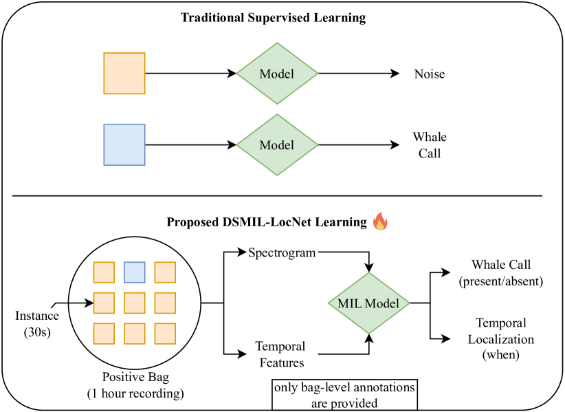
Figure 1: The traditional approach (top) requires instance-level annotations for classification tasks. In contrast, DSMIL-LocNet (bottom) employs a Multiple Instance Learning framework that processes audio recordings as bags containing multiple instances. Spectrogram and temporal features are fed through a dual-stream architecture, the model achieves both classification and temporal localization of whale calls while requiring only bag-level annotations during training. Blue = whale call instance; orange = no call.

Multiple Instance Learning (MIL) [8] offers an alternative framework for automated analysis of PAM data, for tasks like whale call detection where precise instance-level labels are scarce or impractical to obtain. Unlike supervised learning, MIL operates on “bags” of instances, requiring waek labels only at the bag level (e.g., “whale call present/absent” within a 1 hour recording). The instance-level labels (precise call timings) remain latent or unknown and not used during training, making it a weakly supervised learning approach. This characteristic of MIL is well-suited to the challenges of PAM data analysis, where we may know if whale calls are present within a longer recording segment (the bag), but lack precise annotations for each individual call event (the instances). MIL has been applied in audio tasks like acoustic scene classification [9] and sound event detection [10]. However, these applications typically focus on classifying entire audio segments rather than localizing sound events within them. Moreover, most MIL approaches in audio do not explicitly tackle the challenges of long-duration recordings or the need for temporal localization. MIL has also been applied in other domains, including image classification [11], medical analysis [12], and chemical complexity [13].

This work is guided by the following research question:

• RQ1: Can MIL temporally localize whale calls in long recordings using only bag-level labels, without instance-level labels during training?

Building upon this question, we introduce the Dual-Stream Multiple Instance Learning Network for Localization (DSMIL-LocNet), a novel architecture that achieves temporal localization of whale calls using only bag-level labels. DSMIL-LocNet differs from existing MIL approaches in three key ways:

1. Long-Duration Processing: It processes audio bags (2-30 minutes) directly, capturing long-range temporal context unlike short-segment methods.

2. Dual-Stream Architecture: It combines CNN-based spectrogram encoding with MLP-based temporal feature extraction, enhanced by a 4-component loss function balancing classification accuracy, temporal coherence, attention sparsity, and instance consistency.

3. Localization Focus: The attention-based architecture enables both classification and temporal localization, with attention weights providing instance-level relevance within long recordings.

II Method

II-A Problem Definition

Let $\mathcal{A}(t)$ represent a continuous-time audio recording of duration $T$ minutes, segmented into $N$ non-overlapping bags $\{\mathcal{B}_{1},\mathcal{B}_{2},\dots,\mathcal{B}_{N}\}$ of duration $\tau_{b}$ minutes. Each bag $\mathcal{B}_{i}$ contains $M_{i}=\left\lfloor\frac{\tau_{b}}{\tau_{i}}\right\rfloor$ non-overlapping instances $\{\mathbf{x}_{i}^{1},\mathbf{x}_{i}^{2},\dots,\mathbf{x}_{i}^{M_{i}}\}$ of duration $\tau_{i}$. For each instance $\mathbf{x}_{i}^{j}$, timestamp $t_{i}^{j}$ records its start time. A binary bag-level label $y_{i}\in\{0,1\}$ indicates whale vocalization presence, while instance-level labels $y_{i}^{j}\in\{0,1\}$ remain unknown during training. Following standard MIL assumptions:

$$y_{i}=1 \Leftrightarrow\exists j\in\{1,\dots,M_{i}\}:y_{i}^{j}=1$$

$$y_{i}=0 \Leftrightarrow\forall j\in\{1,\dots,M_{i}\}:y_{i}^{j}=0$$

Our goal is to learn a model parameterized by $\boldsymbol{\theta}$ that maximizes $\mathbb{P}(y_{i}|\mathcal{B}_{i};\boldsymbol{\theta})$ subject to $\alpha_{i}^{j}\approx\mathbb{P}(y_{i}^{j}=1|\mathbf{x}_{i}^{j};\boldsymbol{\theta})$, where $\alpha_{i}^{j}$ are attention weights corresponding to latent instance labels. Each instance $\mathbf{x}_{i}^{j}$ is transformed into a $d$ dimesion feature vector $\boldsymbol{\phi}_{i}^{j}\in\mathbb{R}^{d}$ via:

$$\boldsymbol{\phi}_{i}^{j}=f(\mathbf{x}_{i}^{j})=[\boldsymbol{\phi}_{{\text{CNN}}}(\mathbf{S}_{i}^{j}),\mathbf{T}_{i}^{j}].$$

where:

• $\mathbf{S}_{i}^{j}$ is the time-frequency representation (Mel-spectrogram) computed from STFT.

• $\boldsymbol{\phi}_{{\text{CNN}}}$ extracts features from $\mathbf{S}_{i}^{j}$ via a CNN.

• $\mathbf{T}_{i}^{j}$ contains temporal features extracted from $\mathbf{x}_{i}^{j}$.

We define an instance-level prediction function, $h_{\boldsymbol{\theta}}(\mathbf{x}_{i}^{j})$, with attention mechanism:

$$h_{\boldsymbol{\theta}}(\mathbf{x}_{i}^{j})=\sigma(\alpha_{i}^{j}\cdot\boldsymbol{\omega}^{Tr}\boldsymbol{\phi}(\mathbf{x}_{i}^{j})).$$

where $\sigma$ is the sigmoid function, $\boldsymbol{\omega}$ represents the learnable weights, $Tr$ is the transpose operator and $\boldsymbol{\phi}(\cdot)$ is the feature extraction function. The attention weight $\alpha_{i}^{j}$ is computed:

$$\alpha_{i}^{j}=\frac{\exp(\mathbf{v}^{Tr}\tanh(\mathbf{W}\boldsymbol{\phi}(\mathbf{x}_{i}^{j})+\mathbf{b}))}{\sum_{k=1}^{M_{i}}\exp(\mathbf{v}^{Tr}\tanh(\mathbf{W}\boldsymbol{\phi}(\mathbf{x}_{i}^{k})+\mathbf{b}))}\cdot\mu_{i}^{j}.$$

Here, $\mathbf{W}$, $\mathbf{v}$, and $\mathbf{b}$ are learnable, and $\mu_{i}^{j}$ is the binary mask for valid instances. The attention weights are normalized so that the sum of the weights in one bag equals to 1.

The bag-level prediction, $g_{\boldsymbol{\theta}}(\mathcal{B}_{i})$, is a weighted sum of instance embeddings:

$$g_{\boldsymbol{\theta}}(\mathcal{B}_{i})=\sum_{j=1}^{M_{i}}\alpha_{i}^{j}h_{\boldsymbol{\theta}}(\mathbf{x}_{i}^{j}).\vskip-5.69046pt$$

For temporal localization, a detection is made when the attention weight exceeds threshold $\theta$:

$$\mathcal{D}_{i}=\{t_{i}^{j}\mid\alpha_{i}^{j}>\theta,j\in\{1,\dots,M_{i}\}\}.$$

Given ground truth vocalization times $\mathcal{G}_{i}=\{g_{i}^{1},g_{i}^{2},\dots,g_{i}^{K_{i}}\}$, a detection $t_{d}\in\mathcal{D}_{i}$ matches a ground truth time $g_{k}\in\mathcal{G}_{i}$ if: $\lvert t_{d}-g_{k}\rvert\leq\tau$, where $\tau$ is the temporal tolerance threshold and $\lvert\cdot\rvert$ denotes absolute value. Let $\text{card}\{S\}$ denote the cardinality (number of elements) of set $S$. The localization performance is evaluated using:

Precision $$=\frac{\sum_{i}\text{card}\{t_{d}\in\mathcal{D}_{i}\text{ such that }\exists g_{k}\in\mathcal{G}_{i}\text{ with }\lvert t_{d}-g_{k}\rvert\leq\tau\}}{\sum_{i}\text{card}\{\mathcal{D}_{i}\}}$$

Recall $$=\frac{\sum_{i}\text{card}\{g_{k}\in\mathcal{G}_{i}\text{ such that }\exists t_{d}\in\mathcal{D}_{i}\text{ with }\lvert t_{d}-g_{k}\rvert\leq\tau\}}{\sum_{i}\text{card}\{\mathcal{G}_{i}\}}$$

where $\Psi_{i}$ is the set of matched detection-ground truth pairs in bag $i$, and $|\Psi|$ is the total number of matches across all bags. This formulation defines the MIL problem for whale call localization, incorporating feature extraction, attention mechanisms, and the relationship between instance-level and bag-level predictions.

II-B Bag and Instance Creation

Algorithm 1 outlines the hierarchical segmentation of audio recordings into labeled bags of fixed-duration instances through resampling, bandpass filtering, and segmentation. Spectrogram and temporal features are extracted from each instance, and bag-level labels are assigned based on the presence of annotated whale calls.

Algorithm 1 Hierarchical Audio Processing: Recording $\rightarrow$ Bags $\rightarrow$ Instances

1:

2:Audio recording $\mathcal{A}(t)$ with timestamps

3:Ground truth annotations $\mathcal{G}$ with call times

4:Bag duration $\tau_{b}$

5:Instance duration $\tau_{i}$

6:Target sampling rate $f_{s}$ Hz

7:Frequency range $[f_{min},f_{max}]$ Hz

8:procedure ProcessAcousticData($\mathcal{A}(t),\mathcal{G}$)

9:  $a\leftarrow\textsc{Resample}(\mathcal{A}(t),f_{s})$

10:  $a\leftarrow\textsc{BandpassFilter}(a,f_{min},f_{max})$

11:  $N\leftarrow\left\lfloor\frac{\text{length}(a)}{f_{s}\times\tau_{b}}\right\rfloor$ $\triangleright$ Number of bags

12:  for $i\leftarrow 1$ to $N$ do

13:   $t_{start}\leftarrow(i-1)\times\tau_{b}$ $\triangleright$ Bag start time

14:   $\text{bag\_data}\leftarrow a[t_{start}\times f_{s}:(t_{start}+\tau_{b})\times f_{s}]$

15:   $\mathcal{B}_{i}\leftarrow\emptyset$ $\triangleright$ Initialize bag

16:   $y_{i}\leftarrow 0$ $\triangleright$ Initialize bag label

17:   $M_{i}\leftarrow\left\lfloor\frac{\tau_{b}}{\tau_{i}}\right\rfloor$ $\triangleright$ Instances per bag

18:   for $j\leftarrow 1$ to $M_{i}$ do

19:     $t_{i}^{j}\leftarrow t_{start}+(j-1)\times\tau_{i}$ $\triangleright$ timestamp

20:     $\mathbf{x}_{i}^{j}\leftarrow\text{bag\_data}[(j-1)\times\tau_{i}\times f_{s}:j\times\tau_{i}\times f_{s}]$

21:     $S_{i}^{j}\leftarrow\textsc{STFT}(\mathbf{x}_{i}^{j})$

22:     $\boldsymbol{\phi}_{\text{CNN}}\leftarrow\textsc{MelTransform}(S_{i}^{j})$

23:     $\mathbf{T}_{i}^{j}\leftarrow\textsc{TemporalFeatures}(\mathbf{x}_{i}^{j})$

24:     $\boldsymbol{\phi}_{i}^{j}\leftarrow[\boldsymbol{\phi}_{\text{CNN}},\mathbf{T}_{i}^{j}]$

25:     if AnnotationOverlap($t_{i}^{j},t_{i}^{j}+\tau_{i},\mathcal{G}$) then

26:      $y_{i}\leftarrow 1$

27:     end if

28:     $\mathcal{B}_{i}\leftarrow\mathcal{B}_{i}\cup\{(\mathbf{x}_{i}^{j},\boldsymbol{\phi}_{i}^{j},t_{i}^{j})\}$

29:   end for

30:   $\mathcal{B}\leftarrow\mathcal{B}\cup\{(\mathcal{B}_{i},y_{i})\}$

31:  end for

32:  return $\mathcal{B}$

33:end procedure

II-C Network Architecture

DSMIL-LocNet extracts both frequency and time-domain characteristics of whale vocalizations. For each instance $\mathbf{x}_{i}^{j}$, we compute a time-frequency representation $\mathbf{S}_{i}^{j}$:

$$\mathbf{S}_{i}^{j}=\text{MelScale}(|\text{STFT}(\mathbf{x}_{i}^{j})|^{2}).$$

This transformation retains whale call frequency modulation while reducing dimensionality. Temporal features $\mathbf{T}_{i}^{j}$ are extracted as:

$$\mathbf{T}_{i}^{j}=\begin{bmatrix}\text{RMS}(\mathbf{x}_{i}^{j}),&\text{ZCR}(\mathbf{x}_{i}^{j}),&\text{PeakAmp}(\mathbf{x}_{i}^{j}),\\ \text{EnvStats}(\mathbf{x}_{i}^{j}),&\text{TempCentroid}(\mathbf{x}_{i}^{j})\end{bmatrix}$$

where RMS represents root mean square energy, ZCR is the zero-crossing rate, and TempCentroid calculates the temporal center of mass of the signal, along with peak amplitude and envelope statistics (mean, standard deviation). These features capture the temporal structures that distinguish whale calls from background noise.

Our dual-stream architecture processes spectral and temporal features separately. The spectrogram stream $\boldsymbol{\phi}_{{\text{CNN}}}$ employs residual blocks:

$$\mathbf{h}_{l+1}=\mathbf{h}_{l}+F(\mathbf{h}_{l}),\text{ where }F(\mathbf{h}_{l})=\mathbf{W}_{2}\sigma(\text{BN}(\mathbf{W}_{1}\sigma(\text{BN}(\mathbf{h}_{l})))).$$

where $\mathbf{h}_{l}$ represents the feature maps at layer $l$, and $F(\cdot)$ is the residual function, $\mathbf{W}_{1}$ and $\mathbf{W}_{2}$ are convolutional weight matrices, BN denotes batch normalization, and $\sigma$ is the ReLU activation function.

The residual connections maintain gradient flow through deep layers while learning hierarchical spectral features. The temporal stream processes time-domain features:

$$\boldsymbol{\phi}_{\text{temp}}(\mathbf{T}_{i}^{j})=\sigma(\mathbf{W}_{n}\text{BN}(\sigma(\mathbf{W}_{n-1}...\sigma(\mathbf{W}_{1}\mathbf{T}_{i}^{j})))).$$

Our feature fusion module learns to dynamically weight and combine information from both streams:

$$\boldsymbol{\phi}_{i}^{j}=\mathbf{W}_{f}[\boldsymbol{\phi}_{{\text{CNN}}}(\mathbf{S}_{i}^{j});\boldsymbol{\phi}_{{\text{temp}}}(\mathbf{T}_{i}^{j})]+\mathbf{b}_{f}.$$

This fusion allows the model to adapt its feature emphasis based on the signal characteristics, particularly important when dealing with varying noise conditions and call types.

The self-attention processes these fused features:

$$\text{Attention}(\mathbf{Q},\mathbf{K},\mathbf{V})=\text{softmax}\left(\frac{\mathbf{Q}\mathbf{K}^{T}}{\sqrt{d}}\right)\mathbf{V}.\vskip-5.69046pt$$

where $\mathbf{Q}=\mathbf{W}_{q}\boldsymbol{\phi}_{i}^{j}$, $\mathbf{K}=\mathbf{W}_{k}\boldsymbol{\phi}_{i}^{j}$, $\mathbf{V}=\mathbf{W}_{v}\boldsymbol{\phi}_{i}^{j}$, and instance-level attention weight $\alpha_{i}^{j}$:

$$\alpha_{i}^{j}=\text{softmax}(\mathbf{v}^{Tr}\tanh(\mathbf{W}\boldsymbol{\phi}_{i}^{j}+\mathbf{b}))$$

where the softmax operation normalizes attention weights across all instances within bag $i$. During inference, the model produces both bag-level predictions: $g_{\boldsymbol{\theta}}(\mathcal{B}_{i})=\sigma\left(\sum_{j}\alpha_{i}^{j}\boldsymbol{\phi}_{i}^{j}\right)$ and instance-level localization through $\alpha^{j}_{i}$, providing a framework for whale call detection and temporal localization.

II-D Loss Function

Our loss function $\mathcal{L}(\boldsymbol{\theta})$ comprises four components addressing class imbalance, temporal coherence, sparsity, and instance consistency. The primary classification loss uses focal binary cross-entropy:

$$\mathcal{L}_{\text{BCE}}(y_{i},\hat{y}_{i})=-y_{i}(1-\hat{y}_{i})^{\gamma}\log(\hat{y}_{i})-(1-y_{i})\hat{y}_{i}^{\gamma}\log(1-\hat{y}_{i}).$$ (1)

Where $\gamma$ is the focal loss parameter down-weighting, addressing class imbalance in whale call detection with rare positives. Label smoothing with factor $\rho$ adjusts targets to $y_{i}^{\prime}=y_{i}(1-\rho)+\rho/2$.

We add a temporal smoothness constraint for coherent attention across instances, reflecting whale call continuity:

$$\mathcal{L}_{\text{temp}}=\frac{1}{M_{i}}\sum_{i}\sum_{j}(\alpha_{i}^{j}-\alpha_{i}^{j-1})^{2}.$$

As whale calls occupy a small fraction, to ensure selective attention and consistent feature representations, we include sparsity and instance consistency terms:

$$\mathcal{L}_{{\text{sparsity}}}=\frac{1}{M_{i}}\sum_{i}\sum_{j}|\alpha_{i}^{j}|,\mathcal{L}_{{\text{inst}}}=\frac{1}{M_{i}^{2}}\sum_{i}\sum_{j,k}\|\boldsymbol{\phi}_{i}^{j}-\boldsymbol{\phi}_{i}^{k}\|_{2}^{2}.$$

The total loss is a weighted combination of these components:

$$\mathcal{L}(\boldsymbol{\theta})=\mathcal{L}_{{\text{BCE}}}+\lambda_{t}\mathcal{L}_{{\text{temp}}}+\lambda_{s}\mathcal{L}_{{\text{sparsity}}}+\lambda_{i}\mathcal{L}_{{\text{inst}}}.$$ (2)

where $\lambda_{t}$, $\lambda_{s}$, and $\lambda_{i}$ are hyperparameters controlling the contribution of each loss component.

III Experiments

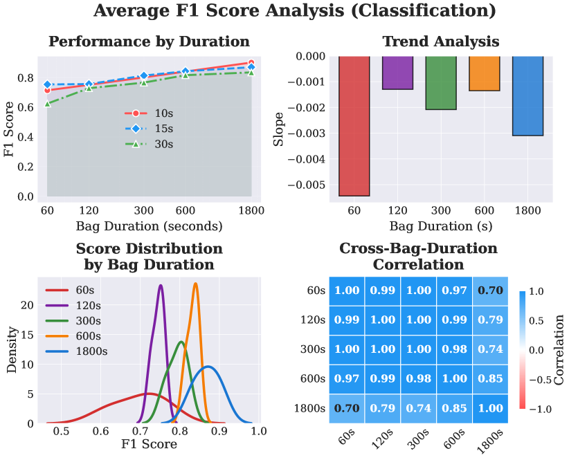
Figure 2: Analysis of classification performance across different bag and instance durations. Results indicate improved performance with longer bags

III-A Dataset

We utilize the AcousticTrends BlueFinLibrary [14], a public dataset of annotated underwater recordings from the Southern Ocean. This dataset comprises 1880.25 hours of audio across seven Antarctic sites and 11 site-year combinations, with annotations indicating the presence of Antarctic blue and fin whale vocalizations. For this study, we framed the task as binary classification (presence/absence of any whale call). The data is highly imbalanced, with a majority (73-99.9%) of recordings containing only background noise. We employed blocked cross-validation, where each site-year combination served as an independent test set in turn, ensuring robust generalization assessment to unseen recording locations and conditions. The remaining site-years were used for training and validation.

III-B Implementation Details

Model implemented in PyTorch using mixed-precision training. We conducted experiments with various bag durations $(60s,120s,300s,600s,1800s)$ and instance durations $(10s,15s,30s)$ to analyze performance impacts. Training used AdamW optimizer (lr=$1e-4$, weight decay=0.01, gradient clipping=1.0), early stopping (patience=15), focal loss ($\gamma$=2.0), label smoothing ($\rho$=0.1), batch size=32, NVIDIA A100 GPU.

III-C Evaluation Metrics and Results

We evaluate using F1 score for classification and precision for temporal localization.

III-C1 Baseline Comparisons

To establish the effectiveness of our approach, we evaluated DSMIL-LocNet against simplified baseline models using a fixed configuration of 300s bag duration and 15s instance duration. Table I summarizes these comparisons. These results demonstrate that our proposed approach outperforms all baseline models in both classification and localization tasks.

TABLE I: Comparison of baseline models with our proposed approach

Model Configuration	Loss Function	F1-Classification	Localization Precision
Temporal-only MIL	$\mathcal{L}_{\text{BCE}}(\ref{eq:bce})$	0.1235	0.4173
Spectrogram-only MIL	$\mathcal{L}_{\text{BCE}}$	0.7391	0.5371
Basic Dual-Stream MIL	$\mathcal{L}_{\text{BCE}}$	0.7880	0.6352
DSMIL-LocNet (Ours)	$\mathcal{L}(\boldsymbol{\theta})(\ref{eq:total})$	0.8133	0.6952

III-C2 Classification Performance

Having established the effectiveness of our approach, we conducted a more detailed analysis of how different temporal parameters affect performance. Figure 2 shows longer bag durations improve classification across all instance durations, with 1800s bags achieving highest F1 scores. This improvement stems from better handling of class imbalance, as longer bags more likely contain whale calls. Trend analysis ($R^{2}$=0.729-0.939) reveals narrowing performance gaps between instance durations as bag duration increases, with intermediate durations (300-600s) showing more stable performance.

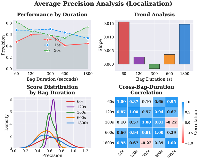
Figure 3: Temporal localization precision across varying bag and instance durations. Optimal performance occurs with shorter bag durations (60-120s) and medium instance lengths (15s), with variability at longer durations.

III-C3 Localization Accuracy

Figure 3 reveals localization follows more complex patterns than classification. Highest precision (0.82) is achieved with 30s instances at 60s bag duration, while 15s instances maintain consistent precision (0.65-0.70) across different bag durations. Variable $R^{2}$ values (0.080-0.995) indicate less predictable instance-duration relationships, with wider score distributions for longer bags suggesting increased variability. The correlation matrix shows weaker and sometimes negative correlations between different bag durations (e.g., -0.22 between 300s and 1800s), highlighting cross-temporal consistency challenges.

III-C4 Performance Trade-offs

1. Instance Duration Effects: The trend analysis slopes show opposing patterns for classification (consistently negative slopes) versus localization (variable slopes), indicating that instance duration impacts these tasks differently.

2. Correlation Structure: The classification correlation matrix shows uniformly high correlations $(\geq 0.97)$ for shorter bag durations, suggesting consistent behavior. In contrast, the localization correlation matrix shows more variable relationships, with some negative correlations, indicating less predictable performance patterns.

3. Distribution: The score distributions show a clear progression toward higher, more concentrated F1 scores with increasing bag duration for classification, while localization precision distributions become more dispersed, indicating reduced reliability in temporal precision.

III-D Comparison with Existing Methods

To the best of our knowledge, DSMIL-LocNet represents the first MIL application to whale call detection and localization in PAM data. Recent approaches have made significant progress in automated whale call detection, but differ fundamentally in their requirements and capabilities. Table II provides a comparative overview of current state-of-the-art methods. While direct performance comparisons are challenging, our high F1 scores and precision demonstrate effectiveness in marine acoustic monitoring, providing both detection and localization within the same framework.

TABLE II: Comparison of Recent Whale Call Detection Methods

Method	Architecture	Input Duration	Features	Annotation	Context
DSMIL-LocNet	Dual-Stream	2-30 min	Spectrogram	Bag	Long-term
(Ours)	MIL + Attn	15s inst.	+ Temporal	(weak)	+ loc.
WT-HMM	HMM	3-26s	Wavelet	Instance	Single
[15]	+ Wavelet			(strong)	call
DenseNet	CNN	4.5s	Spectrogram	Instance	Fixed-
[16]	(Koogu)	(2s OL)		(strong)	window
DeepWhaleNet	ResNet-18	32-131s	Spectrogram	Instance	Multi-
[17]		(50% OL)		(strong)	scale

IV Conclusion

This study investigated whether Multiple Instance Learning could provide an effective framework for analyzing long-duration underwater acoustic recordings while reducing the burden of detailed temporal annotations. Our results demonstrate that incorporating longer temporal contexts through a bag-based approach significantly improves whale call detection accuracy compared to traditional fixed-window methods. DSMIL-LocNet balances the competing demands of broad temporal analysis and precise localization, with longer bag durations improving classification accuracy while maintaining temporal localization through attention-based instance selection. The dual-stream architecture effectively handles challenging marine noise conditions by combining spectral and temporal features. These findings suggest that weak supervision through MIL could transform marine acoustic monitoring, enabling more widespread deployment of automated systems while maintaining necessary precision. While our evaluation focused on whales, the approach can be applied to other species with sparsely structured acoustic signals. Future work should address the challenge of handling diverse acoustic events in complex marine soundscapes, potentially through specialized detectors or multi-class MIL approaches. This work represents a step toward scalable automated monitoring systems for marine conservation and research across multiple species and acoustic event types.

References

- [1] D. K. Mellinger, K. M. Stafford, S. E. Moore, R. P. Dziak, and H. Matsumoto, “An overview of fixed passive acoustic observation methods for cetaceans,” Oceanography, vol. 20, no. 4, pp. 36–45, 2007.
- [2] D. K. Mellinger and C. W. Clark, “Recognizing transient low-frequency whale sounds by spectrogram correlation,” The Journal of the Acoustical Society of America, vol. 107, no. 6, pp. 3518–3529, 2000.
- [3] D. K. Mellinger, “A comparison of methods for detecting right whale calls,” Canadian Acoustics, vol. 32, no. 2, pp. 55–65, 2004.
- [4] A. N. Allen, M. Harvey, L. Harrell, A. Jansen, K. P. Merkens, C. C. Wall, J. Cattiau, and E. M. Oleson, “A convolutional neural network for automated detection of humpback whale song in a diverse, long-term passive acoustic dataset,” Frontiers in Marine Science, vol. 8, p. 607321, 2021.
- [5] Y. Shiu, K. Palmer, M. A. Roch, E. Fleishman, X. Liu, E.-M. Nosal, T. Helble, D. Cholewiak, D. Gillespie, and H. Klinck, “Deep neural networks for automated detection of marine mammal species,” Scientific reports, vol. 10, no. 1, p. 607, 2020.
- [6] E. Schall, I. I. Kaya, E. Debusschere, P. Devos, and C. Parcerisas, “Deep learning in marine bioacoustics: a benchmark for baleen whale detection,” Remote Sensing in Ecology and Conservation, 2024.
- [7] D. Stowell, “Computational bioacoustics with deep learning: a review and roadmap,” PeerJ, vol. 10, p. e13152, 2022.
- [8] M.-A. Carbonneau, V. Cheplygina, E. Granger, and G. Gagnon, “Multiple instance learning: A survey of problem characteristics and applications,” Pattern Recognition, vol. 77, pp. 329–353, 2018.
- [9] W.-G. Choi, J.-H. Chang, J.-M. Yang, and H.-G. Moon, “Instance-level loss based multiple-instance learning framework for acoustic scene classification,” Applied Acoustics, vol. 216, p. 109757, 2024.
- [10] H. Song, J. Han, S. Deng, and Z. Du, “Acoustic scene classification by implicitly identifying distinct sound events,” in Proc. Interspeech 2019, 2019, pp. 3860–3864.
- [11] M. Ilse, J. Tomczak, and M. Welling, “Attention-based deep multiple instance learning,” in International conference on machine learning. PMLR, 2018, pp. 2127–2136.
- [12] G. Quellec, G. Cazuguel, B. Cochener, and M. Lamard, “Multiple-instance learning for medical image and video analysis,” IEEE reviews in biomedical engineering, vol. 10, pp. 213–234, 2017.
- [13] D. Zankov, T. Madzhidov, A. Varnek, and P. Polishchuk, “Chemical complexity challenge: Is multi-instance machine learning a solution?” Wiley Interdisciplinary Reviews: Computational Molecular Science, vol. 14, no. 1, p. e1698, 2024.
- [14] B. S. Miller, “An open access dataset for developing automated detectors of antarctic baleen whale sounds and performance evaluation of two commonly used detectors,” Scientific Reports, vol. 11, no. 1, p. 806, 2021.
- [15] O. P. Babalola and J. Versfeld, “Wavelet-based feature extraction with hidden markov model classification of antarctic blue whale sounds,” Ecological Informatics, vol. 80, p. 102468, 2024.
- [16] N. Rasmussen, R. Rizk, O. Matoo, and K. Santosh, “Deepwhalenet: Climate change-aware fft-based deep neural network for passive acoustic monitoring,” International Journal of Pattern Recognition and Artificial Intelligence, vol. 38, no. 14, p. 2459014, 2024.
- [17] B. S. Miller, S. Madhusudhana, M. G. Aulich, and N. Kelly, “Deep learning algorithm outperforms experienced human observer at detection of blue whale d-calls: a double-observer analysis,” Remote Sensing in Ecology and Conservation, vol. 9, no. 1, pp. 104–116, 2023.