Learning-Based Leader Localization for Underwater Vehicles With Optical-Acoustic-Pressure Sensor Fusion

Abstract

Underwater vehicles have emerged as a critical technology for exploring and monitoring aquatic environments. The deployment of multi-vehicle systems has gained substantial interest due to their capability to perform collaborative tasks with improved efficiency. However, achieving precise localization of a leader underwater vehicle within a multi-vehicle configuration remains a significant challenge, particularly in dynamic and complex underwater conditions. To address this issue, this paper presents a novel tri-modal sensor fusion neural network approach that integrates optical, acoustic, and pressure sensors to localize the leader vehicle. The proposed method leverages the unique strengths of each sensor modality to improve localization accuracy and robustness. Specifically, optical sensors provide high-resolution imaging for precise relative positioning, acoustic sensors enable long-range detection and ranging, and pressure sensors offer environmental context awareness. The fusion of these sensor modalities is implemented using a deep learning architecture designed to extract and combine complementary features from raw sensor data. The effectiveness of the proposed method is validated through a custom-designed testing platform. Extensive data collection and experimental evaluations demonstrate that the tri-modal approach significantly improves the accuracy and robustness of leader localization, outperforming both single-modal and dual-modal methods.

I Introduction

Underwater vehicles, including Autonomous Underwater Vehicles (AUVs) and Remotely Operated Vehicles (ROVs), have revolutionized the exploration and monitoring of aquatic environments [1], [2], [3], [4]. These vehicles provide unprecedented access to deep-sea regions that are otherwise inaccessible to human divers or traditional survey methods. As the capabilities of these vehicles continue to evolve, multi-vehicle systems, also known as underwater vehicle swarms, have emerged as a promising approach to enhance the efficiency and effectiveness of underwater missions. Multi-vehicle systems, comprising multiple underwater vehicles operating collaboratively, enable a wide range of tasks, such as seabed mapping [5], [6], environmental monitoring [7], [8], and marine exploration [9], [10]. By leveraging the strengths of individual underwater vehicles, swarms typically cover larger areas, share computational and sensing resources, and improve overall mission resilience [11], [12].

Despite these advantages, a critical challenge in deploying underwater vehicle swarms is achieving effective relative localization of leader vehicles within the multi-agent system. Accurate relative localization is crucial for maintaining formation stability, ensuring safe navigation, and enabling precise coordination among vehicles [13], [14]. Researchers have investigated various techniques for relative localization, including optical, acoustic, and pressure sensor-based approaches [15], [16].

Optical sensors, such as cameras, provide high-resolution imaging for precise relative positioning in close proximity. For instance, Hong et al. [17] developed the Shark underwater vehicle, achieving vision-based hovering control for underwater inspection tasks. Similarly, Manzanilla et al. [18] designed an autonomous navigation algorithm leveraging single-camera feedback. Acoustic sensors, on the other hand, offer long-range detection and are well-suited for environments with limited visibility. Dos Santos et al. [19] proposed a cross-domain image matching method, integrating aerial and underwater acoustic images for localization tasks. Xu et al. [20] introduced a localization algorithm using forward-looking sonar to estimate the motion of a deep-sea mining vehicle, achieving accurate real-time results. Pressure sensors, which measure ambient water pressure, provide valuable data on depth and environmental context. Wang et al. [21] demonstrated the use of pressure sensors to sense propeller wake for leader-follower formation, utilizing a deep learning network to estimate lateral motion states. Zheng et al. [22] addressed the state estimation of robotic fish in various motions using a lateral line system comprised of distributed pressure sensors.

While each sensor modality provides distinct advantages, underwater environments are inherently dynamic and complex, characterized by time-varying currents, limited visibility, and obstacles, which limit the performance and robustness of single-sensor systems. Researchers have explored dual-modality methods to address these limitations by combining two sensor types to improve localization accuracy. For instance, integrating optical and ultrasonic sensors provides both visual and acoustic information, enabling target localization even in turbid or low-light conditions. Yang et al. [23] proposed a localization method assimilating optical and acoustic measurements, while Song et al. [24] introduced an acoustic-visual approach for underwater navigation. Similarly, combining vision and pressure sensors offers depth information alongside optical images, improving localization precision. Hu et al. [25] developed a visual-pressure fusion method to mitigate large-scale errors in monocular visual-inertial odometry, and Ma et al. [26] proposed a tightly coupled monocular-pressure fusion technique for localizing biomimetic robotic mantas.

However, dual-modality systems, while advantageous over single-modality, often fail to fully exploit the complementary nature of all available sensor types. This limitation underscores the potential of tri-modal fusion methods. By integrating data from optical, acoustic, and pressure sensors, these methods offer a more holistic and accurate perception of the leader’s position, advancing the state of the art in underwater relative localization.

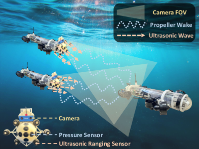
Figure 1: Illustration of an underwater vehicle swarm utilizing the proposed multi-modal leader vehicle localization framework. The visual camera operates within the camera’s field of view (FOV), the acoustic ranging sensors function within their transmission and reception angles, and the pressure sensors respond to detectable propeller wake. Visual cameras (yellow), acoustic ranging sensors (orange), and pressure sensors (blue) collectively gather information about the leader vehicle to estimate its states of interest.

This paper presents a novel tri-modal fusion algorithm that integrates optical, acoustic, and pressure sensors to localize the leader underwater vehicle within a multi-vehicle system. An envisioned underwater vehicle swarm is illustrated in Fig. 1. The proposed method leverages the complementary strengths of these sensor modalities to enhance the accuracy and robustness of leader localization. By fusing data from diverse sensors, the algorithm mitigates the limitations of individual modalities, providing reliable position estimates in challenging underwater environments.

The multi-modal sensor fusion is achieved through a deep learning architecture designed to extract and combine complementary features from raw sensor data. Deep learning has demonstrated remarkable capabilities across various domains, such as object detection [27], speech processing [28], and autonomous systems [29], [30], owing to its ability to learn complex patterns and relationships from large datasets. In this paper, deep learning enables effective fusion of multi-modal sensor data, extracting high-level features critical for accurate position estimation [31], [32].

To validate the proposed method, this paper develops a comprehensive testing platform comprising a test pool, a tri-modal sensing module, and a target module. Extensive data collection and experimental evaluations are conducted to assess the algorithm’s performance. The experimental results demonstrate that the tri-modal fusion deep learning method significantly improves position estimation performance and robustness compared to single- and dual-modal approaches. Specifically, the algorithm achieves higher localization accuracy with reduced variance, under noisy and dynamic conditions.

The main contributions of this work are twofold. First, this paper introduces a novel framework that integrates optical, acoustic, and pressure sensors to address the leader underwater vehicle localization challenge. By leveraging the strengths of each sensor modality, the proposed approach outperforms traditional single- and dual-modal methods in position estimation accuracy and robustness. Second, a testing platform is developed, upon which extensive data collection and experimental evaluations validate the proposed tri-modal fusion method. These contributions are expected to advance the state of the art in underwater vehicle swarms, offering a promising solution for diverse underwater missions that require precise coordination in complex and dynamic environments.

II Problem Description

This section presents the problem addressed in this study and describes the development of the testing platform used for experimentally validating the proposed algorithm.

II-A Testing Platform

This paper develops and constructs a testing platform to faciliate the leader underwater vehicle localization experiments. The platform consists of three primary components, including a test pool, a target module and a tri-modal sensing module. The test pool measures 4 m in length, 2 m in width and 0.7 m in depth.

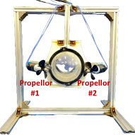
(a) Target module.

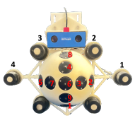
(b) Sensing module.

Figure 2: Illustration of the target module and the tri-modal sensing module. The target module (Fig. 2(a)), supported by an aluminum profile frame, represents the tail section of the leader vehicle with two propellers powered by servo drivers. The tri-modal sensing module (Fig. 2(b)), resembling the head section of the follower vehicle, comprises a 3D-printed support structure, a binocular camera, nine pressure sensors (indexed in red), and six acoustic ranging sensors (indexed in black). Under proper actuation, the propellers in the target module rotate at a constant speed, simulating real-world conditions during underwater vehicle movement and turning. The camera, acoustic ranging sensors, and the pressure sensors in the sensing module capture the associate data, which is subsequently collected for localizing the target module.

The target module, representing the tail section of the leader vehicle and modeled after the OpenAUV, a lab-developed underwater robot [33], is supported by an aluminum profile frame, as illustrated in Fig. 2(a). To capture propeller wake data, two waterproof underwater thrusters (Pasotim 2838) are employed as propellers. The propellers are powered via two Skywolf TL-80 servo drivers, which regulate their rotation direction and speed through pulse-width modulation. The pulse width ranges from 1K to 2K µs, corresponding to the lower and upper control limits, respectively.

The multi-modal sensing module, resembling the head section of the follower vehicle, is secured using an acrylic holder, as illustrated in Fig. 2(b). This module comprises a 3D-printed support structure, a binocular camera mounted at the top, nine pressure sensors centrally located, and six acoustic ranging sensors arranged peripherally. The binocular camera, manufactured by ROVMAKER, supports various resolutions, with a maximum resolution of 2560$\times$960 pixels. The acoustic ranging sensors are 300 KHz Yuzheng04 modules, manufactured by Hangzhou Umbrella Automation Technology. The pressure sensors used are MS5837-02BA, featuring a resolution of 1 Pa and communication via the I2C bus. Real-time acquisition of data from the nine pressure sensors is achieved using three I2C multiplexers from DFRobot. To ensure waterproofing, the MS5837-02BA sensors are enclosed within protective structures. A Raspberry Pi 4B with 8 GB memory is utilized for data acquisition, processing and storage.

II-B Localization Problem

In this study, the leader and follower vehicles are assumed to operate at the same depth, thereby restricting the leader localization problem to the horizontal plane. The test pool features a water depth of 50 cm, with both the target module and the multi-modal sensing module positioned 25 cm below the water surface.

Figure 3: Illustration of the sample locations within the test pool (top view). A mesh grid comprising 42 locations is selected. The fixed multi-modal sensing module is denoted as H, while the target module, represented as T, is manually positioned at each grid vertex. For each location, three orientations of the target module are tested.

As illustrated in Fig. 3, we define the reference frame $I$ within the horizontal plane, the origin denoted as $O$. The $x-$ and $y-$ axes are aligned with the length and width of the test pool, respectively. The displacement of the target module is denoted as $(p_{x},p_{y})$, where $p_{x}$ and $p_{y}$ represent the displacements along $x-$ and $y-$ axes, respectively. In addition, variable $d$ represents the current direction of the leader vehicle. We assume that the leader vehicle takes one of the three possible orientations, namely, towards the left, moving straight (either forward or backward), and towards the right, denoted as $L$, $S$ and $R$, respectively. Thus we have $d\in\{L,S,R\}$. The states of the leader vehicle, denoted as $\bm{s}$, is represented by the vector $\bm{s}=[p_{x},p_{y},d]^{\text{T}}$.

Assume that $P$ acoustic sensors and $Q$ pressure sensors are deployed. Define the measurements of all acoustic sensors at time $k$ as $\bm{m}_{k}^{\text{a}}\in\mathbb{R}^{P}$, and the measurements of all pressure sensors at time $k$ as $\bm{m}_{k}^{\text{p}}\in\mathbb{R}^{Q}$. Additionally, define the 2D camera image captured at time $k$ as $\bm{M}_{k}^{\text{c}}\in\mathbb{R}^{U\times V}$, where $U$ and $V$ denote the width and height of the image, respectively. With the multi-modal measurement data, the estimated states of the leader vehicle at time $k$ is calculated through the estimation algorithm function $f$ by

$$\hat{\bm{s}}_{k}=f(\bm{M}_{k}^{\text{c}},\bm{m}_{k}^{\text{a}},\bm{m}_{k}^{\text{p}}),$$ (1)

At time $k$, define the actual states as $\textbf{{s}}_{k}$, then the absolute estimation error is calculated by

$$e_{k}=\left|\hat{\bm{s}}_{k}-\bm{s}_{k}\right|.$$ (2)

Define the mean Smooth $L_{1}$ Loss [34] as

$$L_{f}=\frac{1}{N}\sum_{k=1}^{N}\left[\frac{1}{2\beta}e_{k}^{2}I_{e_{k}<\beta}+\left(e_{k}-\frac{\beta}{2}\right)I_{e_{k}\geq\beta}\right],$$ (3)

where $N$ is the total quantity of samples, $\beta$ is the threshold hyper-parameter and $I$ is the indicator function.

Finally, the leader state estimation problem is formulated as a task aimed at finding out a function $f^{*}$ that satisfies

$$L_{f^{*}}\leq\epsilon,$$ (4)

where $\epsilon>0$ is the desired loss limit.

III Dataset Construction

This section describes the acquisition process and composition of the multi-modal dataset. First, an overview of the data collection framework is provided, followed by a detailed discussion of the data collection process for each modality.

To ensure comprehensive experimentation, we carefully select a set of sample locations. As illustrated in Fig. 3, a mesh grid consisting of 42 locations is chosen, comprising 7 positions along the $x$-axis and 6 positions along the $y$-axis. Along $x$-axis, marginal space is reserved to allow the target module frame to remain stable and flat, while the rear space along the $y$-axis is maintained to distinguish the acoustic measurement threshold.

The multi-modal sensing module is fixed at $(100,50)$ and denoted as H, while the target module, represented by T, is manually placed at the selected locations and remains stationary during data collection. To simulate the leader vehicle taking different actions, namely turning left, moving straight forward/backward and turning right, the target module is positioned either parallel to the $y$-axis or at angles of $\pm 45^{\circ}$ relative to the $y$-axis. Propellers #1 and #2 are defined as illustrated in Fig. 2(a). The rotation speed and rotation direction (RD), either clockwise (CW) or counterclockwise (CCW), of each propeller are controlled by the supply voltage and servo driver’s pulse width (PW). During the experiment, the supply voltage is maintained at a constant 15 V with minor variances caused by water flow disturbances. The relationship between target module’s actions and the propeller configurations (the servo driver’s pulse width PM and the rotation direction RD) is summarized in Table I.

TABLE I: Propeller Configurations for Target Module’s Actions

Action	Propeller #1		Propeller #2
	PW (µs)	RD	PW (µs)	RD
Move Straight	2K	CCW	1K	CW
Turn Left	1K	CW	1K	CW
Turn Right	2K	CCW	2K	CCW

At each of the 42 predefined locations, multi-modal sensory data are collected with the target module oriented in three distinct directions. This results in a total of 126 sampled cases. To ensure clarity in the experiment description, the term location refers to one of the 42 spatial points, while the term case denotes one of the 126 combinations of target module’s locations and orientations.

Given the use of multiple sensors in the experiment, simultaneous data acquisition and signal transmission are ensured through multi-threading on a Raspberry Pi, utilizing various Python libraries to facilitate efficient processing.

In the following sections, a case is represented by the target module’s state $\bm{s}$ in the triplet form $\left(p_{x},p_{y},d\right)$. For example, the case (40,70,$L$) refers to the scenario where the propeller executes a left-turn action at the location (40,70).

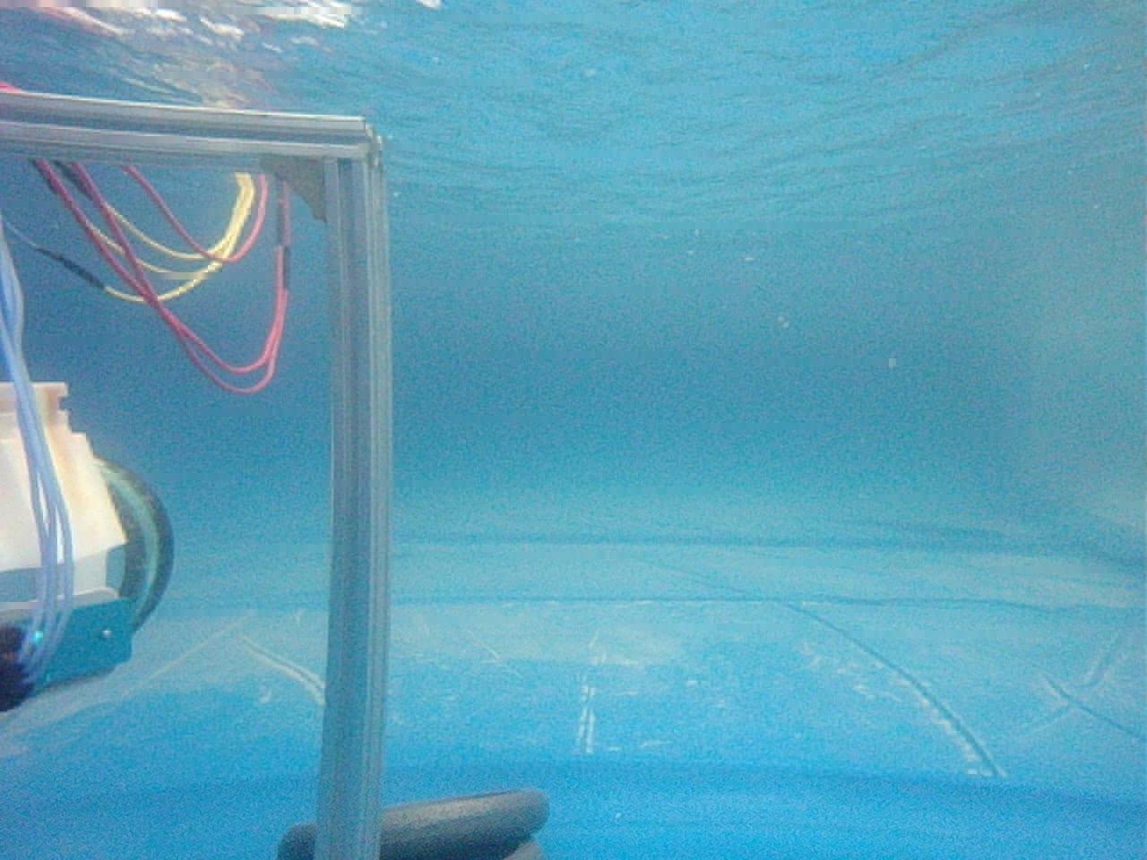
(a) Case (60,90,$M$)

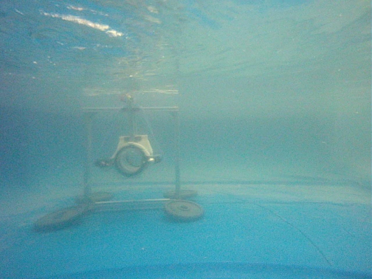
(b) Case (60,190,$M$)

(c) Case (60,290,$M$)

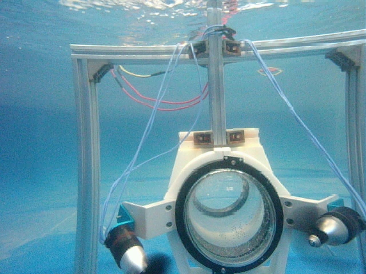
(d) Case (100,90,$M$)

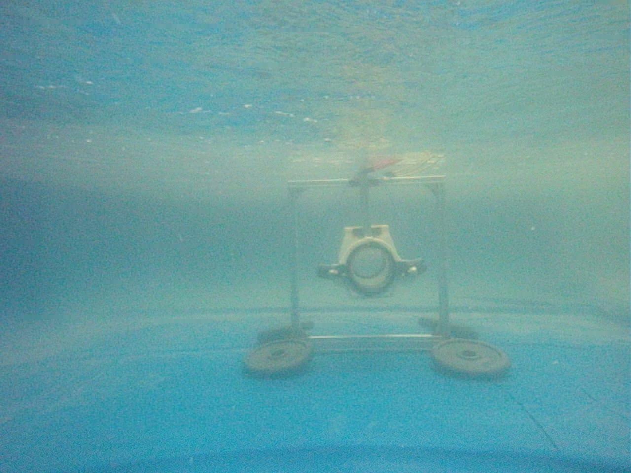
(e) Case (100,190,$M$)

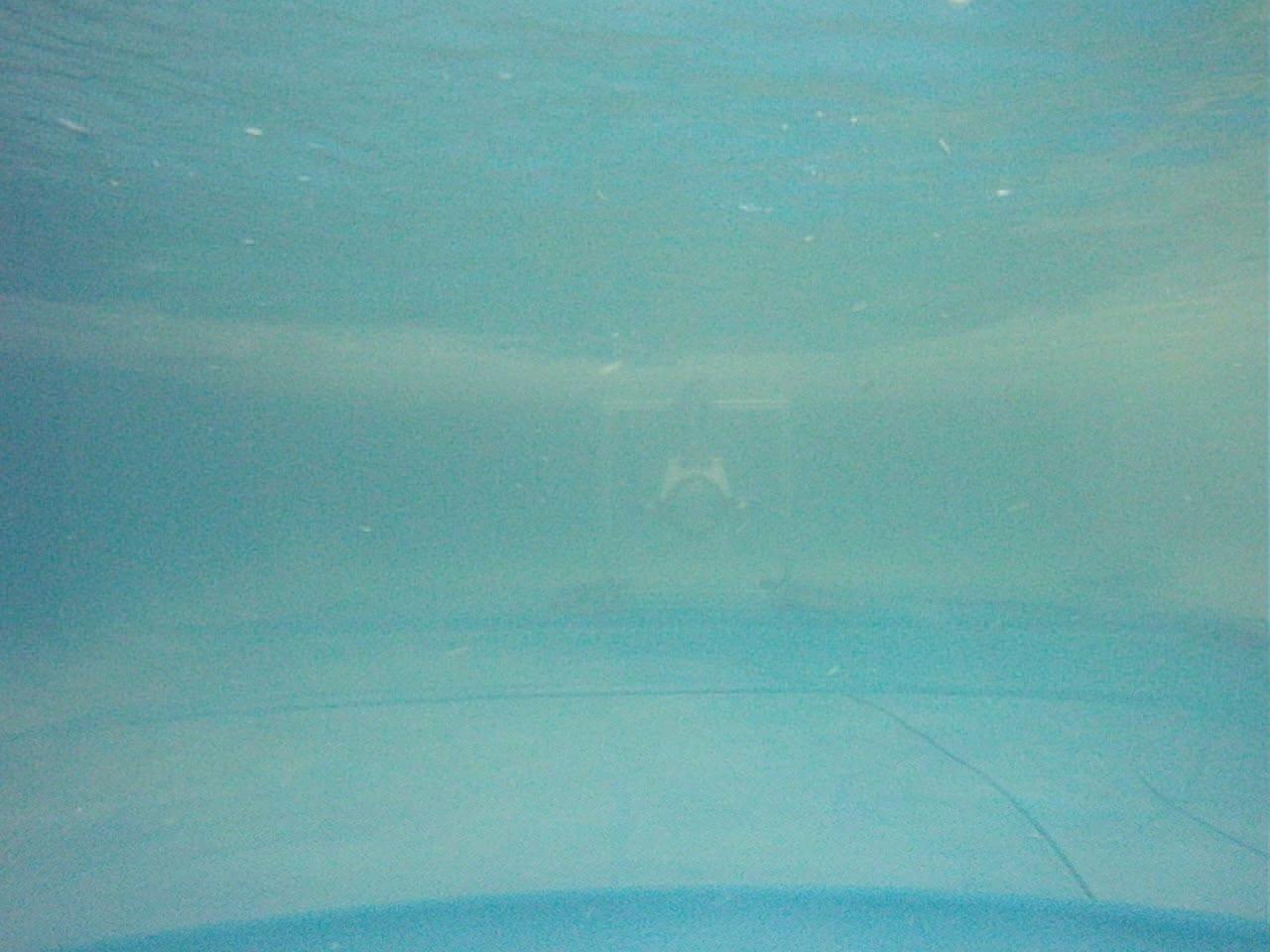
(f) Case (100,290,$M$)

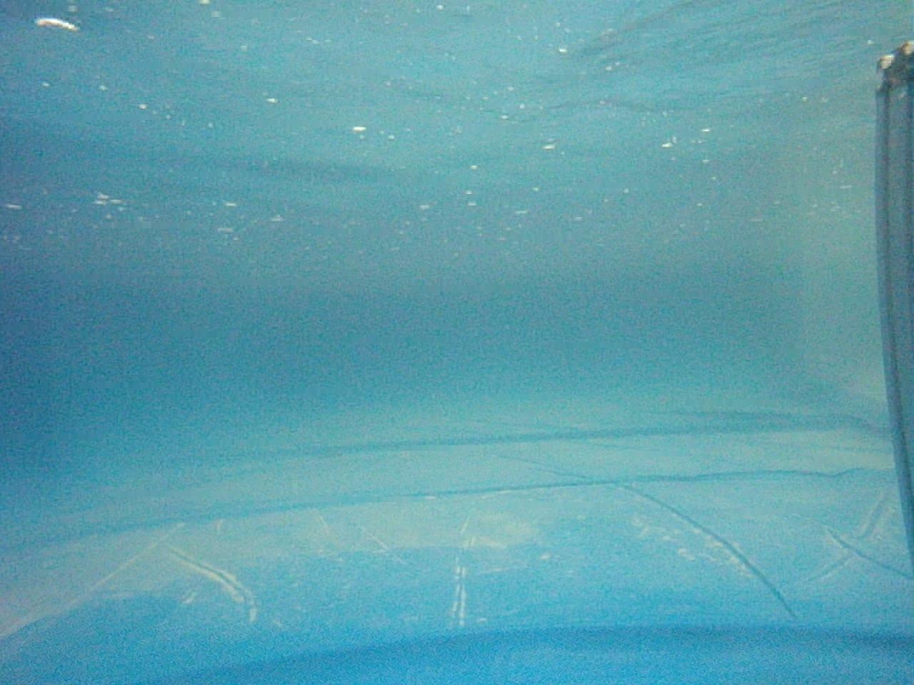
(g) Case (140,90,$M$)

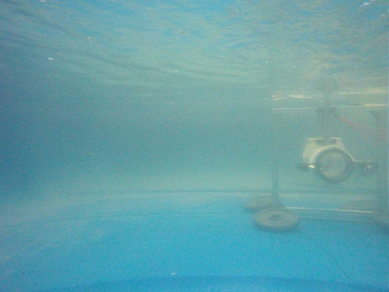
(h) Case (140,190,$M$)

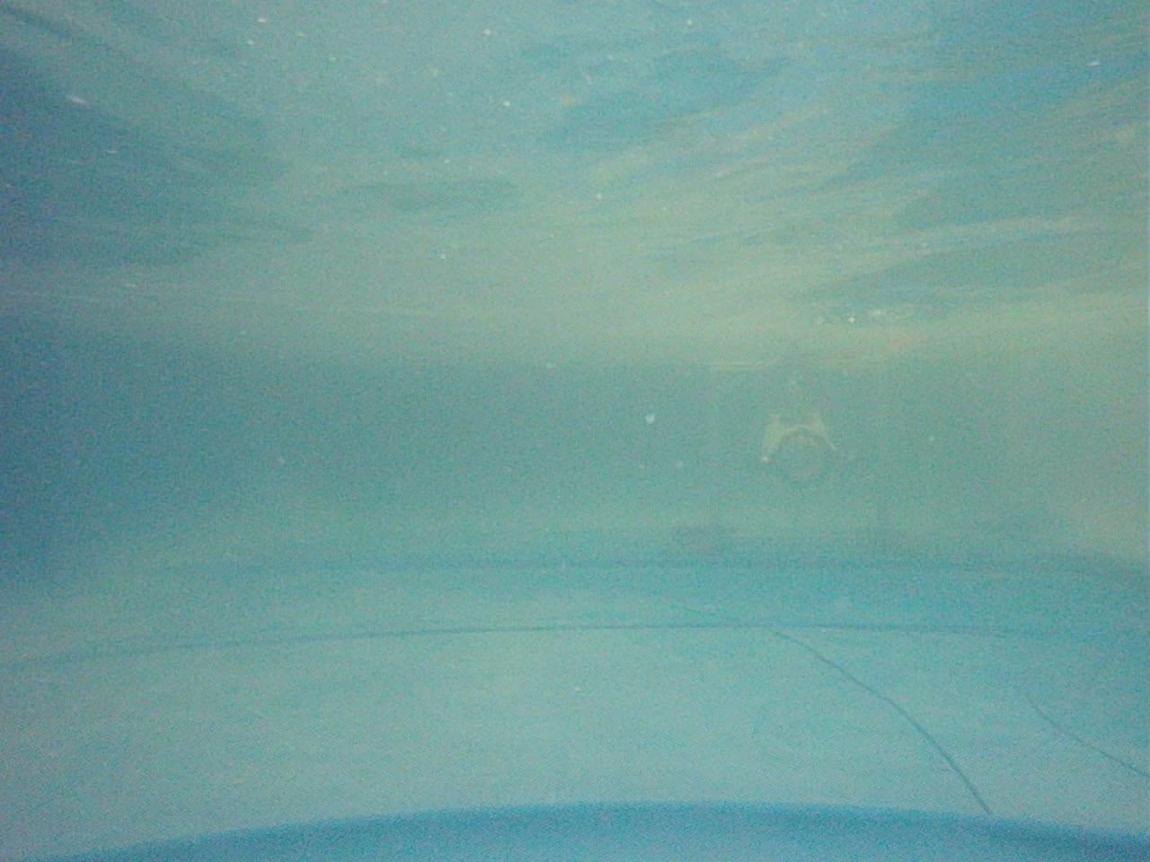
(i) Case (140,290,$M$)

Figure 4: Visualization of the collected raw image data for the provided case triplets.. At $p_{y}=90$ cm, the target appears crystal clear but only partially within the camera field of view (FOV). At $p_{y}=190$ cm, the target is mostly within the camera FOV but less visible. At $p_{y}=290$ cm, the target is fully within in the camera FOV but barely visible due to increased distance and water turbidity.

Visual Data Collection: The camera operates at a sample frequency of 4 fps. For each case, a 12-minute video is recorded, resulting in the collection of approximately 2880 images per case. Fig. 4 visualizes several representative raw images from the collected dataset, annotated with their corresponding case triplets.

Acoustic Data Collection: Four ultrasonic ranging sensors are employed. To mitigate cross-talk issues, the sensors operate sequentially at a sample frequency of 10 Hz each. Fig. 5 illustrates raw acoustic measurements for six cases, with their corresponding states provided. Each demonstrated case spans a duration of 60 seconds. In most instances, the variance in the readings of a specific acoustic sensor decreases as the target module gets closer to the sensing module.

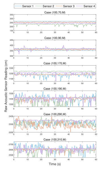
Figure 5: Raw acoustic measurements from four ultrasonic ranging sensors over a 60-second duration for six cases. The case triplets are indicated above each curve plot. When the target is closer to the sensing module, the variance of the readings from a specific acoustic sensor is significantly smaller.

Pressure Data Collection: Nine distributed pressure sensors are used to capture the wake flow of the target module. By optimizing the ms5837 Python library and leveraging multi-threading techniques, a sample frequency of 10 Hz per pressure sensor is achieved. For each case, the nine pressure sensors collaboratively sample the wake generated by the propellers. Prior to propeller operation, still water pressures are recorded for 30 seconds for each case. For each of the 126 cases, denoted as $c$, and sensor $i\in\left[1,2,3,\ldots,9\right]$, the recorded still water measurements are represented by $\left[r_{ci}^{1},r_{ci}^{2},...,r_{ci}^{sl}\right]$. The still water pressure for each case and sensor is calculated by $r^{\text{s}}_{ci}=\frac{1}{L}\sum_{k=1}^{sl}r^{k}_{ci}$, where $sl$ is the sequence length of the still water measurements. At time $k$, the relative pressure sensor reading is calculated by $r^{k^{\prime}}_{ci}=r^{k}_{ci}-r^{\text{s}}_{ci}$. Fig. 6 illustrates the relative pressure sensor readings for six 6 cases, measured in atmospheres (atm). Each illustrated case spans 60 seconds. In general, as the target module moves away from the sensing module along either the $x$-axis or the $y$-axis, fluctuations in the relative pressure sensor readings become less noticeable. Based on the observation, the fluctuations are nearly indistinguishable from background noise when $p_{y}\in\{170,190,290,310\}$. Consequently, pressure sensor data are utilized for target module localization only when $p_{y}\in\{70,90\}$.

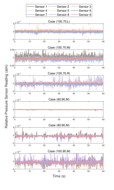
Figure 6: Relative pressure measurements from nine pressure sensors over a 60-second duration. The case triplets are indicated above each curve plot. When the target module moves further from the sensing module along either the $x$-axis or $y$-axis, the fluctuations in the relative pressure sensor readings become weaker.

IV End-to-end State Estimation Algorithm

This section presents a novel end-to-end neural network architecture that fuses three sensing modalities, i.e., visual, acoustic and pressure, to estimate the states of a leader vehicle $\hat{\bm{s}}_{k}$.

The overall design is illustrated in Fig. 7. It comprises five modules including two information fusion modules (highlighted in green) and three feature extraction modules (highlighted in blue). Optical-Acoustic Fusion Module (OAFM) performs data-level fusion of acoustic and optical information. The resulting fused optical-acoustic data, represented as an RGB-Attention (RGBA) image, is processed in the Optical-Acoustic Feature Extraction Module (OAFEM) to extract the optical-acoustic feature (OAF). This feature is subsequently fused with the pressure feature (PF) at the feature level in Optical-Acoustic-Pressure Fusion Module (OAPFM), following processing by the Pressure Feature Extraction Module (PFEM), which outputs the PF. The fused optical-acoustic-pressure feature (OAPF) is then processed by the Optical-Acoustic-Pressure Feature Extraction Module (OAPFEM) to extract the integrated tri-modal feature. The leader state estimation is finally performed based on this tri-modal feature. Detailed designs of these five modules are provided in the following sections.

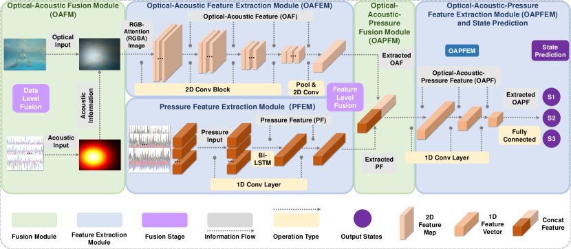
Figure 7: Overview of the end-to-end algorithm architecture for leader vehicle localization. The optical images and the acoustic ranging measurements are fused at the data level (RGBA Image) within the Optical-Acoustic Fusion Module (OAFM). Subsequently, the Optical-Acoustic Feature Extraction Module (OAFEM) applies a sequence of convolutional networks to extract optical-acoustic features (OAF). Pressure sensor measurements are processed through convolutional and recurrent networks in the Pressure Feature Extraction Module (PFEM) to extract pressure features (PF). The extracted OAF and PF are fused at the feature level in the Optical-Acoustic-Pressure Fusion Module (OAPFM). The combined information from all three modalities is processed fully-connected networks in the Optical-Acoustic-Pressure Feature Extraction Module (OAPFEM) to extract the fused optical-acoustic-pressure feature (OAPF), which is used in the final state estimation of the target module.

IV-A Optical-Acoustic Information Fusion (OAFM)

In OAFM, optical information and acoustic information are fused at data level through heatmap attention mechanism.

For most natural images, visual information is stored across the Red, Green and Blue (RGB) channels. However, in certain cases, particularly for images stored in the Portable Network Graphic format, a fourth channel, the Alpha channel, is supported, resulting in an RGBA image. The Alpha channel determines the transparency of the image. The transformation from an RGBA image to an RGB image is governed by [35]

$$v_{j}^{\text{rgb}}=v_{j}^{\text{rgba}}\times v_{\alpha}+v_{j}^{\text{b}}\times(1-v_{\alpha}),$$ (5)

where $j\in${R,G,B}, $v_{j}^{\text{rgb}}$ represents the channel value in the RGB image, $v_{j}^{\text{rgba}}$ represents the corresponding channel value in the RGBA image, $v_{\alpha}$ denotes the value in the Alpha channel, and $v_{j}^{\text{b}}$ represents the RGB value for the background color.

Inspired by the RGBA color model, the OAFM incorporates acoustic information by overlaying it as a heatmap attention channel on the camera’s RGB image, thereby forming an RGB-Attention image, abbreviated as an RGBA image.

The fusion process proceeds as follows. First, Data Preparation. Acoustic ranging sensor data is filtered using upper and lower thresholds. The mean ($\mu_{\text{a}}$) and standard deviation ($\sigma_{\text{a}}$) of the filtered data are calculated, and training/testing data, $r_{\text{a}}$, is generated via a Gaussian distribution, i.e., $r_{\text{a}}\sim N\left(\mu_{\text{a}},\sigma_{\text{a}}^{2}\right)$. Second, Heatmap Generation. Each acoustic sensor’s transmission and reception fields are modeled as a cone beam [36], with uncertainty represented by Gaussian heatmap. Sensor positions relative to the camera are defined by translation vectors $t_{u}^{j}$ and $t_{v}^{j}$. Using $r_{\text{a}}$, boundaries in the image frame ($u_{\text{u}},u_{\text{l}},v_{\text{u}},v_{\text{l}}$) are determined via pinhole camera model transformation $g$. Third, Heatmap Attention. For each acoustic sensor, the mean vector $\bm{\mu}^{j}=\left(\mu_{u}^{j},\mu_{v}^{j}\right)^{\text{T}}$ and covariance matrix $\bm{C}^{j}=$ diag$({\sigma_{u}^{j}}^{2},{\sigma_{v}^{j}}^{2})$ are calculated by $\mu_{u}^{j}=(u_{\text{u}}+u_{\text{l}})/{2}$, $\mu_{v}^{j}=(v_{\text{u}}+v_{\text{l}})/{2}$, $\sigma_{u}^{j}=(u_{\text{u}}-u_{\text{l}})/{\gamma_{u}}$, $\sigma_{v}^{j}=(v_{\text{u}}-v_{\text{l}})/{\gamma_{v}}$, where $\left(\gamma_{u},\gamma_{v}\right)$ are the expansion factors used to control the attention significance. Fourth, Joint Heatmap Fusion. If the target module is within the reception fields of $J$ acoustic sensors, where $2\leq J\leq 4$, individual heatmaps are fused to create a joint heatmap. The joint mean $\bm{\mu}^{\text{J}}=\left(\mu_{u}^{\text{J}},\mu_{v}^{\text{J}}\right)^{\text{T}}$ and joint covariance $\bm{C}^{\text{J}}=$ diag$({\sigma_{u}^{\text{J}}}^{2},{\sigma_{v}^{\text{J}}}^{2})$ are calculated by

$$\mu_{u}^{\text{J}}=\frac{1}{J}\sum_{j=1}^{J}\mu_{u}^{j},\quad\sigma_{u}^{J}=\sqrt{\sum_{j=1}^{J}(\sigma_{u}^{\text{j}})^{2}}$$ (6)

with similar equations for $\mu_{v}^{\text{J}}$ and $\sigma_{v}^{J}$. The fused heatmap is normalized to $\left[0,1\right]$. Last, RGBA Image Formation. The joint acoustic heatmap is concatenated with the corresponding RGB image as an attention channel, forming the RGBA optical-acoustic image.

Examples of RGB images, joint acoustic heatmaps, and fused RGBA images are illustrated in Fig. 8(a), Fig. 8(b), and Fig. 8(c), respectively.

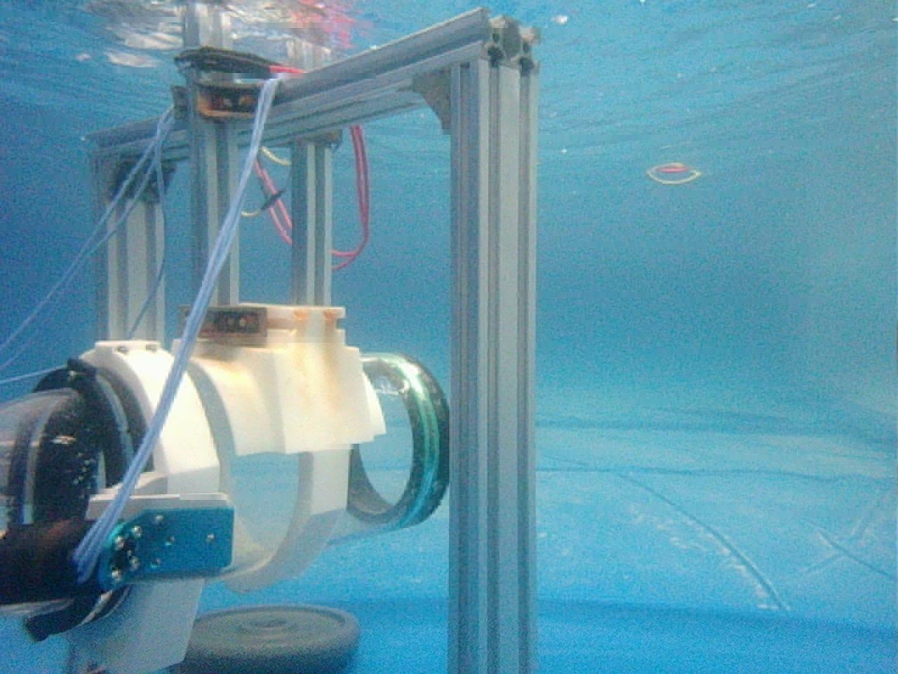
Case (80,90,R)

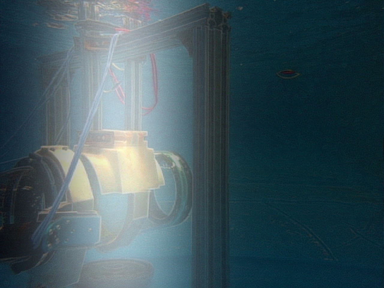
Case (140,190,M)

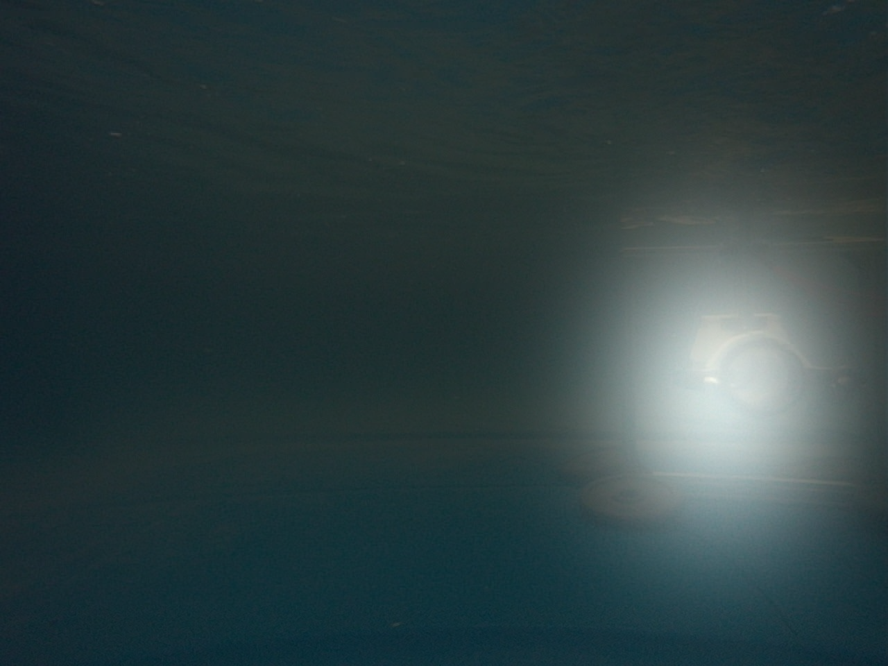
Case (60,290,M)

(a) Camera RGB image.

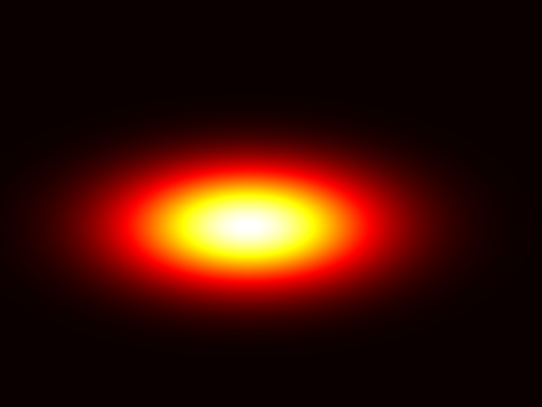
(b) Acoustic heatmap.

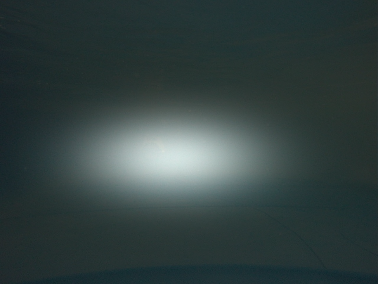
(c) Fused RGBA image.

Figure 8: Visualization of optical-acoustic fusion examples. Each row represents one of three cases. The columns, from left to right, display the camera RGB image, the generated acoustic heatmap, and the fused RGBA image, respectively.

IV-B Optical-Acoustic Feature Extraction (OAFEM)

In OAFEM, G-GhostNet [37, 38], a lightweight CNN, is adopted as the backbone structure. G-GhostNet reduces stage-wise feature redundancy by introducing efficient operations and a mix operation, thus accelerating inference speed. We modified the backbone to suit the OAFEM module’s requirements, with the architecture detailed in Table II, where Block denotes the residual bottleneck specified in [38] and #Out represents the number of output channels. The RGBA input of OAFEM is resized to [224,224] and normalized to [0,1].

TABLE II: Architecture of the OAFEM

Stage	Output Size	Operator	#Out
stem	112$\times$112	Conv$\left(3,3\right)$	16
1	56$\times$56	Block	24
	56$\times$56	Block$\times$1 Cheap	24
	56$\times$56	Concat	24
2	28$\times$28	Block	48
	28$\times$28	Block$\times$3 Cheap	48
	28$\times$28	Concat	48
3	14$\times$14	Block	96
	14$\times$14	Block$\times$3 Cheap	96
	14$\times$14	Concat	96
4	7$\times$7	Block	192
	7$\times$7	Block$\times$5 Cheap	192
	7$\times$7	Concat	192
5	7$\times$7	Conv$\left(1,1\right)$	512
	1$\times$1	Pool & Conv$\left(1,1\right)$	256
	1$\times$1	Conv$\left(1,1\right)$	256

IV-C Pressure Feature Extraction (PFEM)

PFEM is designed to capture the temporal and spatial dependencies within the time-series data of the nine pressure sensor measurements.

To achieve this, a hybrid architecture combining one-dimensional CNN and BiLSTM is employed, enabling the module to effectively extract complex spatiotemporal features of the proeller wake. The 1D CNN excels at uncovering spatial relationships and extracting latent features, while BiLSTM is responsible for learning long-range temporal dependencies. The PFEM comprises four sequential 1D CNN layers followed a BiLSTM layer, as detailed in Table III.

TABLE III: Architecture of the PFEM

Stage	Output Size	Operator	#Out
1	64$\times$1	Conv$\left(3,1\right)$	64
	64$\times$1	Conv$\left(3,1\right)$	64
2	64$\times$1	Conv$\left(3,1\right)$	32
	64$\times$1	Conv$\left(3,1\right)$	32
3	1$\times$1	BiLSTM$\left(128,3\right)$	256
4	1$\times$1	Conv$\left(1,1\right)$	256
	1$\times$1	Conv$\left(1,1\right)$	256

IV-D Optical-Acoustic-Pressure Information Fusion (OAPFM) and Optical-Acoustic-Pressure Feature Extraction (OAPFEM)

In OAPFM, features are concatenated along the channel dimension. Subsequently, OAPFEM employs a series of convolutional layers followed by a fully connected (FC) layer to process the fused features for the final estimation. The architecture design of OAPFM and OAPFEM is detailed in Table IV.

TABLE IV: Architecture of the OAPFM and OAPFEM

Stage	Output Size	Operator	#Out
OAPFM	1$\times$1	Concat	512
OAPFEM	1$\times$1	Conv$\left(1,1\right)$	256
	1$\times$1	Conv$\left(1,1\right)$	128
	1$\times$1	Conv$\left(1,1\right)$	64
Final	1$\times$1	FC	3

IV-E State Estimator

The network outputs three regression values within the range $\left[0,1\right]$, as detailed in Table IV, representing the $x$-axis position $p_{x}$, the $y$-axis position $p_{y}$, and vehicle direction $d$.

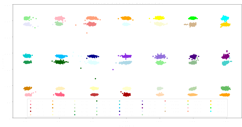
Figure 9: Visualization of position states $(p_{x},p_{y})$ in a scatter plot, excluding the direction state. The horizontal and vertical axes represent the $x$-axis and $y$-axis, respectively, as shown in Fig. 3. Each color corresponds to a location, with each circle representing the estimation result for a test instance. For locations where pressure data is available as an additional information source (i.e., $p_{y}\in\{70,90\}$), the variance in the estimates with the same ground truth is smaller compared to locations with $p_{y}\in\{170,190,290,310\}$, indicating a more accurate and robust state estimation process.

As illustrated in Fig. 3, the absolute $x$ and $y$ coordinates of the sampled locations are $[40,60,80,100,120,140,160]$ cm and $[70,90,170,190,290,310]$ cm, respectively. The position regression values are normalized to [0,1] using $p_{\text{n}}=\left(p-p_{\text{min}}\right)/\left(p_{\text{max}}-p_{\text{min}}\right)$ with $p_{x}\in\left[0,200\right]$ cm and $p_{y}\in\left[0,400\right]$ cm. The normalized $x-$ and $y-$ coordinates, represented by $p_{x\text{n}}$ and $p_{y\text{n}}$, are $[0.2,0.3,0.4,0.5,0.6,0.7,0.8]$ and $[0.175,0.225,0.425,0.475,0.725,0.775]$, respectively. Vehicle direction values, turning left, moving straight, and turning right are represented by 0, 0.5 and 1, respectively.

A smooth $L_{1}$ loss function is adopted for these three states, represented by $l_{\text{x}},l_{\text{y}}$ and $l_{\text{d}}$. The total estimation loss is calculated by $l_{\text{t}}=\lambda_{\text{x}}l_{\text{x}}+\lambda_{\text{y}}l_{\text{y}}+\lambda_{\text{d}}l_{\text{d}}$, where $\lambda_{\text{x}},\lambda_{\text{y}}$ and $\lambda_{\text{d}}$ are weight factors used to balance the significance between the three states.

V Experiments

V-A Training Environment and Hyper-parameters

In the training process, the batch size is set to 128, with a maximum of 200 epochs. The learning rate is set to 0.1 initially and decays by a fctor of 10 every 30 epochs. Stochastic Gradient Descent (SGD) is adopted for optimization. To mitigate overfitting, weight decay and dropout techniques are applied. The training and testing processes are implemented on a desktop computer equipped with NVIDIA GeForce RTX 3070 GPU and an Intel Core i7-12700F CPU.

V-B Results and Discussion

To evaluate the effectiveness of the proposed leader state estimation algorithm, extensive experiments are conducted. Each case utilizes 600 images for training and 200 images for testing. The sequence length of pressure data is set to 64, with values sampled every 0.5 seconds. To enhance the generalization performance of the algorithm, the corresponding acoustic ranging data for each image is generated following a Gaussian distribution $r_{\text{a}}\sim N\left(\mu_{\text{a}},\sigma_{\text{a}}^{2}\right)$, as described in Section IV-A.

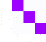
Figure 10: Confusion matrices of estimation result $\hat{d}$ using different modalities. For cases where $p_{y}\in\{70,90\}$, optical, acoustic and pressure information are used for estimation, the confusion matrix is demonstrated in Fig. 10. For cases where $p_{y}\in\{170,190,290,310\}$, only optical and acoustic information are used for estimation, the confusion matrix is demonstrated in Fig. 10.

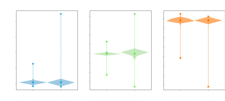
Figure 11: Visualization of the direction state $d$ in a violin plot. The summarized results for ‘Turn Left’, ‘Move Straight’ and ‘Turn Right’ are presented from left to right in three figures with blue, green and orange, respectively. The circle, upper triangle and lower triangle represent the mean value, lower extrema and upper extrema, respectively. Light blue, light green and light orange demonstrate the estimation distributions of the corresponding cases. The horizontal axis represents the modalities used in the estimation process. For cases where $p_{y}\in\{70,90\}$, optical, acoustic and pressure information are used for estimation and the summary result is demonstrated on the left of each pair. For cases where $p_{y}\in\{170,190,290,310\}$, only optical and acoustic information are used for estimation and the summary result is demonstrated on the right of each pair. The vertical axis represents the direction state estimates. The ground truth values of ‘Turn Left’, ‘Move Straight’ and ‘Turn Right’ are 0, 0.5 and 1, respectively.

The regression results for $p_{x}$ and $p_{y}$ are visualized in Fig. 9 with each circle representing a test instance. Each of the 42 locations is assigned a unique color. Table V presents the statistical results, listing the Root Mean Square Error (RMSE) and Standard Deviation (SD) for the estimated states $\hat{p_{x}}$, $\hat{p_{y}}$, and $\hat{d}$. For $p_{y}\in\{70,90\}$, all three modalities are used, whereas for $p_{y}\in\{170,190,290,310\}$, only optical and acoustic sensor measurements are available.

For $d$, thresholds are applied to filter out outliers, and the estimation value $\hat{d}$ is classified as ‘Turn Left’ ($\hat{d}<=0.25$), ‘Move Straight’ ($0.25<\hat{d}<0.75$) and ‘Turn Right’ ($\hat{d}>=0.75$). The confusion matrices, illustrated in Fig. 10, demonstrate that precision and recall values are both over $99\%$ for all cases, whether two or three modalities are used. Incorporating the pressure modality yields an average improvement of $0.03\%$ among all three actions.

After removing outliers, the regression results for $d$ are visualized in the violin plot in Fig. 11. The standard deviation of the estimation value distribution is $15\%$ smaller when all three modalities are utilized compared to when only two modalities are used, indicating improved robustness. Additionally, the mean values (represented by blue, green and orange circles) are closer to the ground truth when all three modalities are used, indicating better accuracy. When all three modalities are used, the average absolute error between the predicted mean values and the corresponding ground truths is reduced by 0.00018 for all three actions. Furthermore, among the predicted output value of all test cases, for all three directional actions, the lower extrema are greater, and for two out of three actions, the upper extrema are smaller when all three modalities are employed. The mean values, upper and lower extrema are listed in Table VI.

TABLE V: Statistical Results of Proposed Method

Modality	Condition	$\hat{p_{x}}$		$\hat{p_{y}}$		$\hat{d}$
		RMSE	SD	RMSE	SD	RMSE	SD
Optical+Acoustic+Pressure	$p_{y}\in\{70,90\}$	$0.00464$	$0.00372$	$0.00339$	$0.00336$	$0.00761$	$0.00699$
Optical+Acoustic	$p_{y}\in\{170,190,290,310\}$	$0.00498$	$0.00466$	$0.00444$	$0.00435$	$0.00859$	$0.00818$
Overall	$p_{y}\in\{70,90,170,190,290,310\}$	$0.00487$	$0.00437$	$0.00412$	$0.00405$	$0.00803$	$0.00766$

TABLE VI: Mean, upper and lower extrema for direction prediction

Action	Mean		Lower Extrema		Upper Extrema
	Optical+Acoustic	Optical+Acoustic	Optical+Acoustic	Optical+Acoustic	Optical+Acoustic	Optical+Acoustic
		+Pressure		+Pressure		+Pressure
Turn Left	$0.00390$	$0.00364$	$-0.00821$	$-0.00791$	$0.20792$	$0.07421$
Move Straight	$0.49967$	$0.50007$	$0.32362$	$0.38731$	$0.71077$	$0.57105$
Turn Right	$0.99589$	$0.99591$	$0.82180$	$0.89858$	$1.00519$	$1.01247$

• When predicting with three modalities, all three mean values are closer to ground truth, all three lower extrema are larger and two out of three upper extrema are smaller, indicating a better overall prediction performance.

TABLE VII: Statistical Results of Ablation Study

Modality	Condition	$\hat{p_{x}}$		$\hat{p_{y}}$		$\hat{d}$
		RMSE	SD	RMSE	SD	RMSE	SD
Pressure	$p_{y}\in\{70,90\}$	$0.02221$	$0.02100$	$0.01846$	$0.01834$	$0.16593$	$0.14242$
Optical	$p_{y}\in\{70,90\}$	$0.00641$	$0.00619$	$0.00630$	$0.00555$	$0.01129$	$0.01119$
Optical	$p_{y}\in\{170,190,290,310\}$	$0.00664$	$0.00638$	$0.00679$	$0.00592$	$0.01165$	$0.01136$
Optical Overall	$p_{y}\in\{70,90,170,190,290,310\}$	$0.00657$	$0.00632$	$0.00665$	$0.00581$	$0.01156$	$0.01131$

V-C Ablation Study

To highlight the advantages of the proposed tri-modal fusion method, this section presents comparison experiments, contrasting leader localization results using tri-modal and single-modal sensory data.

V-C1 Single-modal-based State Prediction

In this section, pure RGB-based and pressure based state estimation results are summarized and analyzed.

RGB-Based State Estimation: This subsection demonstrates the results of estimating the leader’s states using only optical information. The analysis covers all 126 cases, corresponding to $p_{y}\in\{70,90,170,190,290,310\}$. The OAFEM backbone structure is employed for model training and testing. The model input consists of RGB images, while the output matches that of the proposed algorithm, comprising three regression states. The training and testing environment, as well as the hyperparameters, remain the same. Statistical results are summarized in Table VII.

Pressure-Based State Estimation: This subsection presents the result of estimating the leader’s states using only pressure information. This analysis is limited to cases where pressure data is effective, specifically for $p_{y}\in\{70,90\}$. The PFEM backbone structure is utilized for the training and testing process. The model input consists solely pressure measurement sequences, and the outputs are the three regression states. The training and testing environment, as well as the hyperparameters are kept consistent. Statistical results are detailed in Table VII.

Using optical data alone, the RMSE and SD values for all three states are approximately 1.5 times larger than their tri-modal counterparts. With pressure data alone, the estimation results show significantly larger errors compared to the tri-modal approach. For $\hat{p_{x}}$ and $\hat{p_{y}}$, the RMSE and SD are 4 to 6 times higher, while for $\hat{d}$, these values are 20 times greater.

V-C2 Dual-modal-based State Prediction

For cases where $p_{y}\in\{170,190,290,310\}$, only optical and acoustic information, i.e. RGBA image, is used for state prediction. For all three states, the RMSE and SD values increase by an average of $17.06\%$ and $23.92\%$, respectively, when pressure modality is unavailable, as shown in Table V.

The inclusion of pressure information reduces RMSE and SD by an average of $5.31\%$ and $6.49\%$, respectviely, for all estimated states. Among them, $\hat{p_{y}}$ achieves the lowest RMSE (0.00412) and SD (0.00405), followed closedly by $\hat{p_{x}}$. The largest RMSE and SD values are observed for $\hat{d}$, approximately twice those of the other states, yet they remain within an acceptable range, as illustrated in Figs. 10 and 11.

This comprehensive comparison of state estimation results using single-modal, dual-modal, and tri-modal inputs verifies the effectiveness of the proposed algorithm in terms of both accuracy and robustness.

VI Conclusion

This paper presented a tri-modal fusion approach to address the critical challenge of localizing a leader vehicle within multiple-vehicle systems operating in demanding underwater environments. By integrating optical, acoustic, and pressure sensor measurements within a deep neural network framework, the proposed method achieved significant improvements in state estimation accuracy and robustness. The fusion process was systematically structured into two stages. At the data level, acoustic and optical information are combined by constructing an RGB-Attention image. This image integrated a heatmap, representing the Gaussian distribution of acoustic sensor data, with the RGB camera image along the channel dimensions. At the feature level, optical-acoustic and pressure feature were extracted using convolutional and LSTM blocks and subsequently fused to generate leader state estimates. A comprehensive testing platform was developed to evaluate the proposed approach. Extensive experimental results, including comparison studies against single-modal and dual-modal sensing experiments, validated its effectiveness.

For future research, we plan to deploy the proposed tri-modal sensor fusion design onto underwater vehicles and evaluate its performance in real-world underwater environments. Additionally, we will investigate optimizations to the configuration and arrangement of these multi-modal sensors to enhance their relative localization performance within underwater vehicle swarms.

References

- [1] N. Palomeras, N. Hurtós, E. Vidal, and M. Carreras, “Autonomous exploration of complex underwater environments using a probabilistic next-best-view planner,” IEEE Robotics and Automation Letters, vol. 4, no. 2, pp. 1619–1625, 2019.
- [2] U. K. Verfuss, A. S. Aniceto, D. V. Harris, D. Gillespie, S. Fielding, G. Jiménez, P. Johnston, R. R. Sinclair, A. Sivertsen, S. A. Solbø et al., “A review of unmanned vehicles for the detection and monitoring of marine fauna,” Marine pollution bulletin, vol. 140, pp. 17–29, 2019.
- [3] D. Sward, J. Monk, and N. Barrett, “A systematic review of remotely operated vehicle surveys for visually assessing fish assemblages,” Frontiers in Marine Science, vol. 6, p. 134, 2019.
- [4] S. Raine, R. Marchant, B. Kusy, F. Maire, and T. Fischer, “Point label aware superpixels for multi-species segmentation of underwater imagery,” IEEE Robotics and Automation Letters, vol. 7, no. 3, pp. 8291–8298, 2022.
- [5] E. Galceran and M. Carreras, “Efficient seabed coverage path planning for asvs and auvs,” in 2012 IEEE/RSJ International Conference on Intelligent Robots and Systems, 2012, pp. 88–93.
- [6] Q. Wang, B. He, Y. Zhang, F. Yu, X. Huang, and R. Yang, “An autonomous cooperative system of multi-auv for underwater targets detection and localization,” Engineering Applications of Artificial Intelligence, vol. 121, p. 105907, 2023.
- [7] C. Lodovisi, P. Loreti, L. Bracciale, and S. Betti, “Performance analysis of hybrid optical–acoustic auv swarms for marine monitoring,” Future Internet, vol. 10, no. 7, p. 65, 2018.
- [8] A. Vasilijević, . Nađ, F. Mandić, N. Mišković, and Z. Vukić, “Coordinated navigation of surface and underwater marine robotic vehicles for ocean sampling and environmental monitoring,” IEEE/ASME Transactions on Mechatronics, vol. 22, no. 3, pp. 1174–1184, 2017.
- [9] J. Zhang, G. Han, J. Sha, Y. Qian, and J. Liu, “Auv-assisted subsea exploration method in 6g enabled deep ocean based on a cooperative pac-men mechanism,” IEEE Transactions on Intelligent Transportation Systems, vol. 23, no. 2, pp. 1649–1660, 2021.
- [10] Y. Li, M. Ma, J. Cao, G. Luo, D. Wang, and W. Chen, “A method for multi-auv cooperative area search in unknown environment based on reinforcement learning,” Journal of Marine Science and Engineering, vol. 12, no. 7, p. 1194, 2024.
- [11] C. Wang, D. Mei, Y. Wang, X. Yu, W. Sun, D. Wang, and J. Chen, “Task allocation for multi-auv system: A review,” Ocean Engineering, vol. 266, p. 112911, 2022.
- [12] Y.-L. Chen, X.-W. Ma, G.-Q. Bai, Y. Sha, and J. Liu, “Multi-autonomous underwater vehicle formation control and cluster search using a fusion control strategy at complex underwater environment,” Ocean Engineering, vol. 216, p. 108048, 2020.
- [13] Y. Li, K. Cai, Y. Zhang, Z. Tang, and T. Jiang, “Localization and tracking for auvs in marine information networks: Research directions, recent advances, and challenges,” IEEE Network, vol. 33, no. 6, pp. 78–85, 2019.
- [14] Q. Wei, Y. Yang, X. Zhou, C. Fan, Q. Zheng, and Z. Hu, “Localization method for underwater robot swarms based on enhanced visual markers,” Electronics, vol. 12, no. 23, p. 4882, 2023.
- [15] Y. Cong, C. Gu, T. Zhang, and Y. Gao, “Underwater robot sensing technology: A survey,” Fundamental Research, vol. 1, no. 3, pp. 337–345, 2021.
- [16] D. Q. Huy, N. Sadjoli, A. B. Azam, B. Elhadidi, Y. Cai, and G. Seet, “Object perception in underwater environments: a survey on sensors and sensing methodologies,” Ocean Engineering, vol. 267, p. 113202, 2023.
- [17] L. Hong, X. Wang, D.-S. Zhang, M. Zhao, and H. Xu, “Vision-based underwater inspection with portable autonomous underwater vehicle: Development, control, and evaluation,” IEEE Transactions on Intelligent Vehicles, vol. 9, no. 1, pp. 2197–2209, 2024.
- [18] A. Manzanilla, S. Reyes, M. Garcia, D. Mercado, and R. Lozano, “Autonomous navigation for unmanned underwater vehicles: Real-time experiments using computer vision,” IEEE Robotics and Automation Letters, vol. 4, no. 2, pp. 1351–1356, 2019.
- [19] M. Machado Dos Santos, G. G. De Giacomo, P. L. J. Drews, and S. S. C. Botelho, “Matching color aerial images and underwater sonar images using deep learning for underwater localization,” IEEE Robotics and Automation Letters, vol. 5, no. 4, pp. 6365–6370, 2020.
- [20] W. Xu, J. Yang, H. Wei, H. Lu, X. Tian, and X. Li, “A localization algorithm based on pose graph using forward-looking sonar for deep-sea mining vehicle,” Ocean Engineering, vol. 284, p. 114968, 2023.
- [21] J. Wang, D. Zhao, Y. Zhao, F. Zhang, and T. Shen, “Estimating the lateral motion states of an underwater robot by propeller wake sensing using an artificial lateral line,” IEEE/ASME Transactions on Mechatronics, pp. 1–10, 2024.
- [22] X. Zheng, W. Wang, M. Xiong, and G. Xie, “Online state estimation of a fin-actuated underwater robot using artificial lateral line system,” IEEE Transactions on Robotics, vol. 36, no. 2, pp. 472–487, 2020.
- [23] M. Yang, Z. Sha, and F. Zhang, “A multimodal approach based on large vision model for close-range underwater target localization,” IEEE/ASME Transactions on Mechatronics, pp. 1–11, 2024.
- [24] J. Song, W. Li, and X. Zhu, “Acoustic-vins: Tightly coupled acoustic-visual-inertial navigation system for autonomous underwater vehicles,” IEEE Robotics and Automation Letters, vol. 9, no. 2, pp. 1620–1627, 2024.
- [25] C. Hu, S. Zhu, Y. Liang, Z. Mu, and W. Song, “Visual-pressure fusion for underwater robot localization with online initialization,” IEEE Robotics and Automation Letters, vol. 6, no. 4, pp. 8426–8433, 2021.
- [26] S. Ma, J. Wang, Y. Huang, Y. Meng, M. Tan, J. Yu, and Z. Wu, “Tightly coupled monocular-inertial-pressure sensor fusion for underwater localization of a biomimetic robotic manta,” IEEE Transactions on Instrumentation and Measurement, vol. 73, pp. 1–11, 2024.
- [27] S. Xu, M. Zhang, W. Song, H. Mei, Q. He, and A. Liotta, “A systematic review and analysis of deep learning-based underwater object detection,” Neurocomputing, vol. 527, pp. 204–232, 2023.
- [28] D. W. Otter, J. R. Medina, and J. K. Kalita, “A survey of the usages of deep learning for natural language processing,” IEEE Transactions on Neural Networks and Learning Systems, vol. 32, no. 2, pp. 604–624, 2021.
- [29] J. Fayyad, M. A. Jaradat, D. Gruyer, and H. Najjaran, “Deep learning sensor fusion for autonomous vehicle perception and localization: A review,” Sensors, vol. 20, no. 15, p. 4220, 2020.
- [30] S. Kuutti, R. Bowden, Y. Jin, P. Barber, and S. Fallah, “A survey of deep learning applications to autonomous vehicle control,” IEEE Transactions on Intelligent Transportation Systems, vol. 22, no. 2, pp. 712–733, 2020.
- [31] F. Maurelli, S. Krupiński, X. Xiang, and Y. Petillot, “Auv localisation: a review of passive and active techniques,” International Journal of Intelligent Robotics and Applications, vol. 6, no. 2, pp. 246–269, 2022.
- [32] S. Ding, T. Zhang, M. Lei, H. Chai, and F. Jia, “Robust visual-based localization and mapping for underwater vehicles: A survey,” Ocean Engineering, vol. 312, p. 119274, 2024.
- [33] Z. Sha, X. Wang, M. Yang, H. Lei, and F. Zhang, “A portable autonomous underwater vehicle with multi-thruster propulsion: Design, development, and vision-based tracking control,” IEEE Robotics and Automation Letters, pp. 1–8, 2025.
- [34] R. Girshick, “Fast r-cnn,” in 2015 IEEE International Conference on Computer Vision (ICCV), 2015, pp. 1440–1448.
- [35] A. R. Smith, “Alpha and the history of digital compositing,” Citeseer, Tech. Rep., 1995.
- [36] Z. Qiu, Y. Lu, and Z. Qiu, “Review of ultrasonic ranging methods and their current challenges,” Micromachines, vol. 13, no. 4, p. 520, 2022.
- [37] K. Han, Y. Wang, Q. Tian, J. Guo, C. Xu, and C. Xu, “Ghostnet: More features from cheap operations,” CoRR, vol. abs/1911.11907, 2019. [Online]. Available: http://arxiv.org/abs/1911.11907
- [38] K. Han, Y. Wang, C. Xu, J. Guo, C. Xu, E. Wu, and Q. Tian, “Ghostnets on heterogeneous devices via cheap operations,” CoRR, vol. abs/2201.03297, 2022. [Online]. Available: https://arxiv.org/abs/2201.03297