Structural breaks detection and variable selection in dynamic linear regression via the Iterative Fused LASSO in high dimension

Abstract

We aim to develop a time series modeling methodology tailored to high-dimensional environments, addressing two critical challenges: variable selection from a large pool of candidates, and the detection of structural break points, where the model’s parameters shift. This effort centers on formulating a least squares estimation problem with regularization constraints, drawing on techniques such as Fused LASSO and AdaLASSO, which are well-established in machine learning. Our primary achievement is the creation of an efficient algorithm capable of handling high-dimensional cases within practical time limits. By addressing these pivotal challenges, our methodology holds the potential for widespread adoption. To validate its effectiveness, we detail the iterative algorithm and benchmark its performance against the widely recognized Path Algorithm for Generalized Lasso. Comprehensive simulations and performance analyses highlight the algorithm’s strengths. Additionally, we demonstrate the methodology’s applicability and robustness through simulated case studies and a real-world example involving a stock portfolio dataset. These examples underscore the methodology’s practical utility and potential impact across diverse high-dimensional settings.

1 Introduction

Time series models with exogenous variables are extensively applied across diverse fields such as economics, business, finance, environmental studies, and health. These models fulfill two primary objectives: analyzing the dynamics of a variable to identify influential factors, and forecasting the variable’s future evolution. Despite their widespread use, the practical application of these models is hampered by major challenges: selecting relevant variables, and identifying structural breaks.

The challenge of variable selection, often referred to as determining the "model structure," has traditionally been addressed through the sequential application of statistical tests [2]. While effective for small-scale problems (fewer than 100 variables), these methods become impractical in high-dimensional contexts where the number of candidate variables exceeds the available sample size [4]. In such scenarios, alternative approaches from machine learning, particularly regularization techniques, have proven invaluable. These methods estimate coefficients by minimizing the squared error while incorporating penalties on the magnitude of the coefficients. Ridge Regression [5] was among the first of these techniques, though it does not perform variable selection, as all coefficients remain non-zero. The introduction of LASSO [7] marked a significant breakthrough, enabling efficient handling of a large number of variables. This was later refined by methods such as AdaLASSO [10], which improved performance in variable selection and model fitting.

Another critical issue in time series modeling is the identification of structural breaks, moments when the coefficients, or even the set of relevant variables, undergo significant changes. In finance, dynamic regression models used to replicate active investment fund strategies must account for corresponding changes in regression coefficients over time. Extensive econometric research addresses structural breaks, from seminal works such as [3] to more recent studies like [6]. However, as with variable selection, these methods are largely based on repeated statistical tests, limiting their applicability to low-dimensional settings. In high-dimensional contexts, the literature remains underdeveloped, particularly in addressing the simultaneous challenges of variable selection and structural breaks. The Fused LASSO [8], which implements a "trend filter," offers a partial solution by modeling trends in coefficients but does not extend to the inclusion of explanatory variables. This limitation has motivated our current work, which seeks to address these gaps in high-dimensional time series modeling.

We propose a new variation of the modeling that identifies structural breaks and detects change points in high-dimensional settings. As a result, we find a model with fewer parameters to estimate and greater power in identifying these parameters. The novelty we bring is a solution procedure that uses the properties of Fused LASSO iteratively to compare adjacent observations, allowing us to identify structural breaks, identify relevant variables and discard irrelevant ones.

The paper is organized as follows. Sections 2, 3, and 4 establish the theoretical foundations of regularized regression, framing these approaches as optimization problems. In Section 5, we present the most effective solution currently available, which addresses the problem by solving its dual formulation. Section 6 introduces our novel algorithm, explaining how it achieves faster and less biased solutions to the proposed problem. Subsection 6.1 details the application of the proposed solution to the structural break problem, while Subsection 6.2 describes its associated algorithms. In Section 7, we present the results of our experiments. Finally, Section 8 concludes the paper.

2 LASSO (Least Absolute and Shrinkage and Selection Operator)

Given the inputs $\mathbf{X}=(x_{1},\cdots,x_{n})\in\mathbb{R}^{n\times p}$ and the response variable $y=(y_{1},\cdots,y_{n})\in\mathbb{R}^{n}$, LASSO [7] finds the solution $(\hat{\beta_{0}},\hat{\beta})$ to the optimization problem in its Lagrangian form:

$$\begin{array}[]{ll}\hat{\beta}^{LASSO}=\operatorname*{arg\,min}\limits_{\beta}&\biggl{\{}{\sum}_{i=1}^{n}\biggl{(}y_{i}-{\sum}_{j=1}^{p}x_{ij}\beta_{j}\biggl{)}^{2}+\quad\lambda\;{\sum}_{j=1}^{p}|\beta_{j}|\biggl{\}}\\ \end{array}$$ (1)

where $\lambda$ is a tuning parameter, for some $\lambda\geq 0$. The solutions, however, may be inconsistent when there is high correlation among predictor variables and does not possess Oracle properties.

3 Adaptive LASSO (AdaLASSO)

The Adaptive LASSO [10] is better than LASSO regarding variable selection consistency, bias reduction, and achieving Oracle properties, especially in complex scenarios with large numbers of predictors or collinearity. The Adaptive LASSO is designed to possess Oracle properties under certain regularity conditions. This means that, as the sample size increases, the Adaptive LASSO can correctly identify the true model with high probability, leading to better asymptotic performance. Using an initial estimate $\tilde{\beta}$, which solves the optimization problem in its Lagrangian form:

$$\begin{array}[]{ll}\hat{\beta}^{AdaLASSO}=\operatorname*{arg\,min}\limits_{\beta}&\biggl{\{}{\sum}_{i=1}^{n}\biggl{(}y_{i}-{\sum}_{j=1}^{p}x_{ij}\beta_{j}\biggl{)}^{2}+\quad\lambda{\sum}_{j=1}^{p}\omega_{j}|\beta_{j}|\biggl{\}}\\ \end{array}$$ (2)

where $\lambda$ is a tuning parameter, and $\omega_{j}=1/|\tilde{\beta}_{j}|^{\nu}$. If $p<n$, least squares solutions can be used as the initial estimates. When $p\geq n$, least squares estimates are undefined, so the Ridge solution can be used as an initial estimate.

4 Fused LASSO

The Fused LASSO, [8], exploits a piecewise-constant structure within a signal and is the solution to the following optimization problem in its Lagrangian form:

$$\begin{array}[]{ll}\hat{\beta}^{FusedLASSO}=\operatorname*{arg\,min}\limits_{\beta}&\biggl{\{}{\sum}_{i=1}^{n}\biggl{(}y_{i}-{\sum}_{j=1}^{p}x_{ij}\beta_{j}\biggl{)}^{2}+\;\lambda_{1}{\sum}_{j=1}^{p}|\beta_{j}|\;+\;\lambda_{2}{\sum}_{j=2}^{p}|\beta_{j}-\beta_{j-1}|\biggl{\}}\\ \end{array}$$ (3)

Here, $\lambda_{1}$ and $\lambda_{2}$ are tuning parameters. The first penalty, based on the $\ell_{1}$ norm, shrinks the $\beta_{i}$ coefficients towards zero, promoting sparsity. The second penalty leverages the ordered nature of the data, encouraging neighboring $\beta_{i}$ coefficients to be similar and often identical. While the fused LASSO provides a significant advantage over the adaptive LASSO by incorporating relationships among sequentially ordered variables, it is restricted to modeling relationships only between adjacent variables.

5 Path Algorithm for Generalized Lasso Problems

We now focus on a competing algorithm that detects and models the structural break problem, the Path Algorithm for Generalized Lasso (genlasso). Building on analogue $LASSO$ and Fused $LASSO$ frameworks, [9]. It penalizes the $\ell_{1}$ norm of a matrix $D$ times the coefficient vector. The algorithm is based on solving the dual of the generalized lasso, which facilitates computation of the path. Considering the generalized LASSO problem:

$$\min_{\beta}\frac{1}{2}||y-X\beta||_{2}^{2}+\lambda||D\beta||_{1}$$

here $D$ is a penalty matrix that may encode a graph $E$ structure, where each row of $D$ corresponds to an edge, penalizing differences between connected nodes in the graph. The Path Algorithm introduces a graph-based approach leveraging the generalized lasso problem, tailored for graph structures where nodes represent data points and edges impose penalties reflecting differences between connected nodes. Using properties of the conjugate function and the Fenchel-Young inequality one can derive the dual problem as:

$$\begin{array}[]{ll}\min\limits_{u}&f(-D^{T}u)\\ \text{s.t.}\\ &||u||_{\infty}\leq\lambda\\ &u\succeq 0\\ \end{array}$$ (4)

In this context, the generalized LASSO promotes piecewise constant solutions, encouraging neighboring nodes in the graph to adopt similar or identical values. This results in fused regions where connected nodes share nearly uniform values. The computational framework, based on the dual of the problem, ensures efficient path computation of the primal optimization problem in its Lagrangian form (5):

$$\begin{array}[]{ll}\hat{\beta}^{GenLASSO}=\operatorname*{arg\,min}\limits_{\beta}&\biggl{\{}{\sum}_{i=1}^{n}\biggl{(}y_{i}-{\sum}_{j=1}^{p}x_{ij}\beta_{j}\biggl{)}^{2}+\quad\lambda{\sum}_{(i,j)\in E}^{p}|\beta_{i}-\beta_{j}|+\quad\gamma\lambda{\sum}_{i=1}^{p}|\beta_{i}|\biggl{\}}\\ \end{array}$$ (5)

Here, $\lambda>0$ is a tuning parameter and $\gamma\in[0,1]$, promote sparsity and encourages neighboring coefficients to be similar and often identical.

6 Iterative Fused LASSO

We propose a novel extension to the fused LASSO, broadening its scope to account for time varying parameters. To identify all recurring states for each feature, we propose an iterative procedure that leverages the Adaptive LASSO to determine if there exists at least one of the $p$ components of $\beta_{i,j}$ such that $\beta_{i,j}=\beta_{i-1,j}$. We want to solve the problem (6).

$$\begin{array}[]{ll}\hat{\beta}^{IFL}=\operatorname*{arg\,min}\limits_{\beta_{i,j}}&\biggl{\{}{\sum}_{i=1}^{n}\biggl{(}y_{i}-{\sum}_{j=1}^{p}x_{i,j}\beta_{i,j}\biggl{)}^{2}+\;\lambda_{0}{\sum}_{i=1}^{n}{\sum}_{j=1}^{p}|\beta_{i,j}|\;+\;\lambda_{1}{\sum}_{i=2}^{n}{\sum}_{j=1}^{p}|\beta_{i,j}-\beta_{i-1,j}|\biggl{\}}\\ \end{array}$$ (6)

here $\lambda_{0}$ and $\lambda_{1}$ are tuning parameters. The first penalty serves to shrink the $\beta_{i,j}$ coefficients towards zero, while the second penalty encourages $\beta_{i,j}$ and $\beta_{i-1,j}$ coefficients to be similar, and will cause some of them to be identical.

6.1 Solving the Structural Break problem

In this scenario, we focus on identifying recurring states in consecutive observations, specifically when $\beta_{i,j}=\beta_{i-1,j}$. If any feature $j$ exhibits a state change between two observations, such that $\beta_{i,j}\neq\beta_{i-1,j}$, for $i=2,\cdots,n$ and $j=1,\cdots,p$, we interpret this as a structural break in the $j$-th feature at the $i$-th observation. To address this, we propose a two-step method: on the first step, it detects if and where structural breaks occur, and then on the second step, it estimates the feature coefficients for each regime. For the first step, let´s consider the Ada LASSO problem (2), written as:

$$\begin{array}[]{ll}\hat{\beta}^{AdaLASSO}=\operatorname*{arg\,min}\limits_{\beta}&(y-X\beta)^{T}(y-X\beta)+\lambda\sum_{j=2}^{p}\omega_{\beta,j}|{\beta_{j}}|\\ \end{array}$$ (7)

where $y$ is the vector of observations, $X$ is the design matrix, $\beta$ is the vector of parameters to be estimated, and $\omega=1/|\tilde{\beta}|^{\nu}$ is the penalization in Adaptive LASSO. We will use $\nu=1$ for simplicity. We rewrite the problem, so the design matrix $X$ takes the form:

$$X=\begin{bmatrix}diag(x_{1})|\cdots|diag(x_{p})\end{bmatrix}=\begin{bmatrix}\begin{bmatrix}\begin{array}[]{ccc}x_{11}&\cdots&0\\ \vdots&\cdots&\vdots\\ 0&\cdots&x_{n1}\\ \end{array}\end{bmatrix}\cdots\begin{bmatrix}\begin{array}[]{ccc}x_{1p}&\cdots&0\\ \vdots&\cdots&\vdots\\ 0&\cdots&x_{np}\\ \end{array}\end{bmatrix}\end{bmatrix}$$

then the vector $\beta$ is:

$$\beta=vec(B)=\begin{bmatrix}\begin{array}[]{c}\beta_{(1)}\\ \beta_{(2)}\\ \vdots\\ \beta_{(p)}\end{array}\end{bmatrix},\quad B=\begin{bmatrix}\begin{array}[]{ccc}\beta^{T}_{11}&\cdots&\beta^{T}_{1p}\\ \vdots&\ddots&\vdots\\ \beta^{T}_{n1}&\cdots&\beta^{T}_{np}\end{array}\end{bmatrix}=\begin{bmatrix}\begin{array}[]{c}\beta^{T}_{1}\\ \vdots\\ \beta^{T}_{n}\end{array}\end{bmatrix}=\begin{bmatrix}\beta_{(1)}\cdots\beta_{(p)}\end{bmatrix}$$

In this problem, $X$ is $(n\times np)$, and $\beta$ is $(np\times 1)$. Our goal is to detect recurring values in each of the $p$ components at observation $i$ of $\beta_{i,j}$, $i=2,\cdots,n$, $j=1,\cdots,p$. To achieve this, we need to define supporting matrices that will help us manage the lag differences between observations and the number of recurring values in each component $p$. Denoting the difference matrix $L_{d}^{(k)}$ for component $p$ as follows: $d$ represents the lag difference between observations, and $k$ represents the number of distinct values in feature $p$.

$$L_{d}^{(k)}=I_{k}-\begin{bmatrix}\begin{array}[]{ll}0_{d,(k-d)}&0_{d,d}\\ I_{(k-d)}&0_{(k-d),d}\end{array}\end{bmatrix}$$

And now we can define the difference matrix, $L_{1}$ as:

$$L_{1}=\begin{bmatrix}\begin{array}[]{ccc}L_{1}^{(k)}&0&0\\ 0&\ddots&0\\ 0&0&L_{1}^{(k)}\end{array}\end{bmatrix}$$

$L_{1}$ is a diagonal matrix that shows the number of distinct values in each one of the $p$ components at one lag difference. This allows us to solve the Structural Break problem:

$$\hat{\beta}^{SB}=\operatorname*{arg\,min}\limits_{\theta}(y-XL_{1}^{-1}\theta)^{T}(y-XL_{1}^{-1}\theta)+\lambda\sum_{i=2}^{p}\omega_{\theta,i}|{\theta_{i}}|$$ (8)

where $L_{1}^{-1}\theta=\beta$, such that $\theta=L_{1}\beta\rightarrow\beta=L_{1}^{-1}\theta$. At this stage, we can assume that each of the $p$ features has distinct values with no repetitions. Given $n$ observations and $p$ features, we can express the following:

$$L_{1}=\begin{bmatrix}\begin{array}[]{ccc}L_{1}^{(n)}&0&0\\ 0&\ddots&0\\ 0&0&L_{1}^{(n)}\end{array}\end{bmatrix},\;\text{and}\;\theta=\begin{bmatrix}\begin{array}[]{c}\beta_{1,1}\\ \beta_{2,1}-\beta_{1,1}\\ \cdots\\ \beta_{1,n}\\ \beta_{2,n}-\beta_{1,n}\\ \cdots\\ \beta_{p,n}-\beta_{p-1,n}\\ \end{array}\end{bmatrix}$$

By solving the Structural Break problem (8), we obtain the solution $\hat{\beta}^{SB}$. The best tuning parameter $\lambda$ is selected using the Bayesian Information Criterion (BIC). The Ada LASSO solution estimates which components of $\beta_{i,j}-\beta_{i-1,j}$ can be set to zero. Components that are non-zero indicate differences between consecutive values, representing a structural break in the time series at observation $i$ for the $j$-th component. However, the Structural Break solution does not estimate the specific values of $\beta_{i,j}$. Instead, it identifies the observations where these values differ, thus indicating where a structural break occurs in the data.

In order to proceed, we propose a procedure that rewrites the problem in a reduced form that takes into account the repeated values of $\beta_{i,j}$ and the breaks found in the $\hat{\beta^{SB}}$ solution of (8). First, we must keep track of all recurring values in each $p$ component. To do this we define $\beta_{in}$, a $p\times 1$ vector, that tracks the number of distinct values at each one of the $p$ components. At the first iteration $\beta_{in}=[n,\cdots,n]$, assuming all $\beta_{i,j}$, $i=2,\cdots,n$ and $j=1,\cdots,p$ are distinct.

After solving equation (8), we obtain $\hat{\beta}^{SB}$. This allows us to identify which of the terms $\beta_{j,i}-\beta_{j,i-1}$ are zero and which are non-zero. Next, we define $\gamma_{d}$, a $np\times 1$ vector that accumulates the number of different values of $\beta_{i,j}$ at each $j$ component, $j=1\cdots,p$. After identifying the number of different values of $\beta_{i,j}$ at each component, we define $\beta_{out}$, a $p\times 1$ vector, that tracks the number of distinct values at each one of the $p$ components. If no repeated values were identified, then $\beta_{out}=\beta_{in}$. Therefore each component of $\beta_{out}$ is at most as high as $\beta_{in}$.

With $\beta_{in}$ and $\beta_{out}$, we are able to reduce the problem in such a way that takes into account all repeated values of $\beta_{i,j}$ identified after solving (8). Let´s define $n_{\beta_{in}}$, the number of different values in $\beta_{in}$ as the sum of its components, and also $n_{\beta_{out}}$, the number of different values in $\beta_{out}$ as the sum of its components. We define a matrix $M$ that has as many lines as the number of different values in $\beta_{in}$, and as many columns as the number of different values in $\beta_{out}$. We build matrix $M$ in such a way that it maps a reduced problem:

$$\min\limits_{\gamma}\frac{1}{2}(y-H\gamma)^{T}(y-H\gamma)+\lambda\sum_{i=1}^{K}\omega_{i}|{\gamma_{i}}|$$ (9)

where $H=[XM]$ and $\gamma=\beta_{reduced}$ ($K\times 1$), and $K$ is the number of distinct features in the reduced model. The reduced problem estimates $\gamma$ such that it takes into account the structural breaks identified in (8) and also produces estimates for $\beta$ that solves (7).

Our proposed procedure estimates $\beta_{i,j}$ for each observation $i=1,\cdots,n$, for each feature $j=1,\cdots,p$, enabling the identification of structural breaks, accurate detection of breakpoints, and proper selection of relevant variables.

6.2 Algorithms used for Mopping the model

At the end of the stage, it is possible to identify elements of $\beta_{i,j}$ that are repeated over time. In the next stage, these values can be estimated, taking into account that they are equal. In order to do this, we will build a vector that accumulates the number of different values of $\beta_{i,j}$ at each $j$ component, $j=1\cdots,p$, and call it $\gamma_{d}$.

Algorithm 1 explains how $\gamma_{d}$ is created. Also we will create a matrix $M$ that maps the mopped $\beta_{reduced}$ to the full $\beta_{i,j}$. This matrix will have columns with $0$s or $1$s that position $\beta_{reduced}$ by pre-multiplying matrix $M$.

Algorithm 2 explains how matrix $M$ is created. Let $n_{\beta_{in}}$ be the sum of different components of $\beta_{in}$, and $n_{\beta_{out}}$ be the sum of different components of $\beta_{out}$.

Algorithm 1 Vector $\gamma_{d}$.
Inputs: ($\beta$, $n$, $p$, $\beta_{in}$, $d$).
Output: vector $\gamma_{d}$

 Initialize $\gamma_{d_{\text{boolean}}}\leftarrow$ abs($\beta$) $>0$

 Initialize $\gamma_{d}\leftarrow\mathbf{0}_{n_{\beta_{in}}\times 1}$

 for $i\leftarrow 0$ to $(n-1)$ do

  for $j\leftarrow 1$ to $p$ do

   if $j\leq d$ then

    $\gamma_{d}[i+j]\leftarrow 1$

   else if $\gamma_{d}[i+j]=$ TRUE then

    $\gamma_{d}[i+j]\leftarrow\gamma_{d}[i+j-1]+1$

   end if

  end for

 end for

 Return $\gamma_{d}$

Algorithm 2 Selection Matrix M.
Inputs: ($\beta$, $\beta_{in}$, $\beta_{out}$, $\gamma_{d}$).
Output: matrix $M$

 Initialize $M\leftarrow\mathbf{0}_{n_{\beta_{in}}\times n_{\beta_{out}}}$

 for $i\leftarrow 1$ to $n_{\beta_{in}}$ do

  if $\gamma_{d}[i]\neq 0$ then

   $M(i,\gamma_{d}[i])\leftarrow 1$

  else

   $M(i,\gamma_{d}[i-d])\leftarrow 1$

  end if

 end for

 Return $M$

7 Numerical examples

Our primary objectives were to correctly select relevant variables, identify structural breaks, and accurately detect breakpoints. To evaluate the performance of our approach, we applied the Iterative Fused LASSO (IFL) algorithm using the GLMNet package in R. As benchmarks, we used solutions generated by the Path Algorithm for Generalized Lasso Problems, implemented via the genlasso package from the CRAN repository, [1].

7.1 Monte Carlo simulation results

The simulated experiments involved generating 18 sets of 100 time series each. For each scenario, we constructed a four-regime sample using distinct sets of design matrices. The experiments varied the total number of features ($p$) and the number of relevant, non-zero features ($q$). Additionally, we examined the effect of varying the number of observations within each regime ($n/R$). The performances of the IFL and GenLASSO solutions were compared for all scenarios, with the Oracle solutions serving as benchmarks.

The simulated scenarios included varying the number of observations per regime ($n/R=30$, $n/R=50$), the total number of features ($p=20$, $p=30$, $p=40$), and the total number of relevant (non-zero) features ($q=2$, $q=5$, $q=10$).

Figures 2 and 2 illustrate examples of the estimated feature values over time for one instance solved using each algorithm. This instance involved $n=200$ observations, $p=30$ features, and $q=5$ non-zero features. In both cases, IFL demonstrated smaller bias and MSE compared to GenLASSO. Notably, the $mopping$ algorithm generated solutions that were less noisy and more closely aligned with the synthesized values.

In all replications of our Monte Carlo experiments the IFL algorithm was able to correctly identify structural breaks, accurately detect breakpoints, and correctly select variables.

Tables 2 and 2 present the results for IFL and GenLASSO, respectively. The average bias and MSE for the Monte Carlo scenarios are summarized. Comparing IFL and GenLASSO across scenarios reveals that for less sparse problems ($q=10$), GenLASSO exhibits lower bias and MSE than IFL. Conversely, for sparser problems ($q=2$), GenLASSO shows higher bias and MSE compared to IFL. Notably, as the number of relevant variables decreases, IFL consistently provides solutions with lower bias than GenLASSO.

Further insights into the performance differences are illustrated in Figures 3 and 4, which display the distribution of the bias for both algorithms alongside the Oracle solution for $n=120$ ($n/R=30$) observations, and $n=200$ ($n/R=50$) observations, with different combinations of candidate and relevant variables. These figures demonstrate that as the number of relevant variables increases, both IFL and GenLASSO tend to deviate more from the Oracle. However, IFL generally remains closer to the Oracle compared to GenLASSO.

A critical observation pertains to the convergence time of each method. Across all solved cases, the IFL algorithm converges in approximately $10\%$ of the time required by GenLASSO. This significant difference renders GenLASSO impractical for larger problems, such as those involving $n\geq 400$ observations.

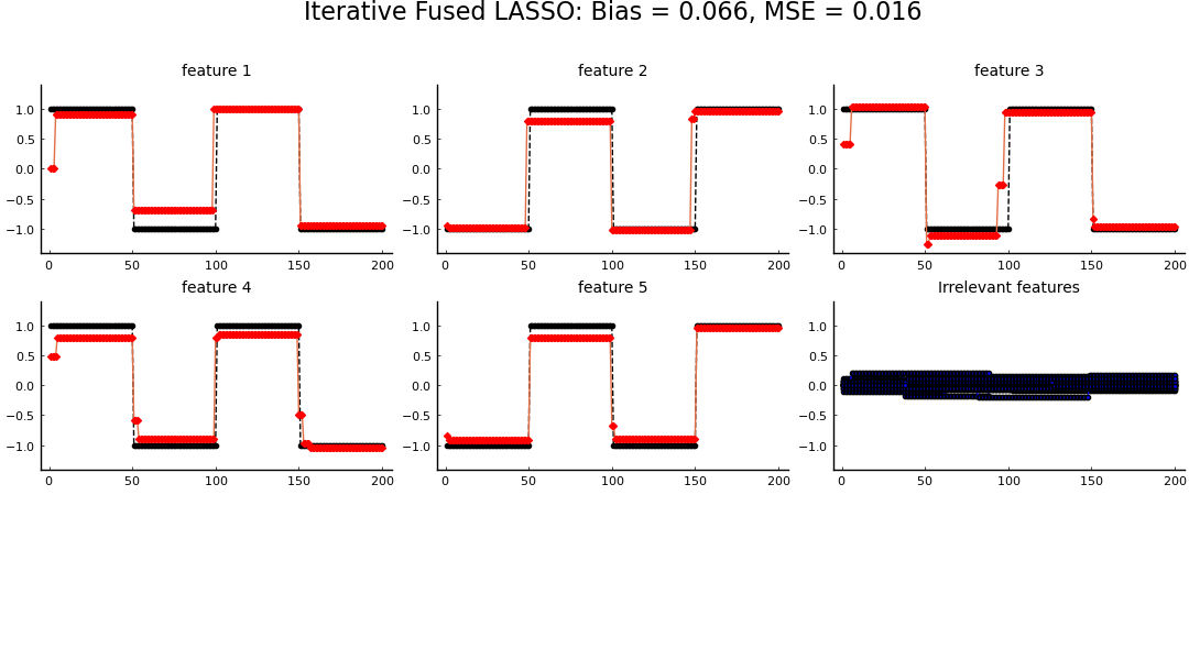
Figure 1: IFL solution example

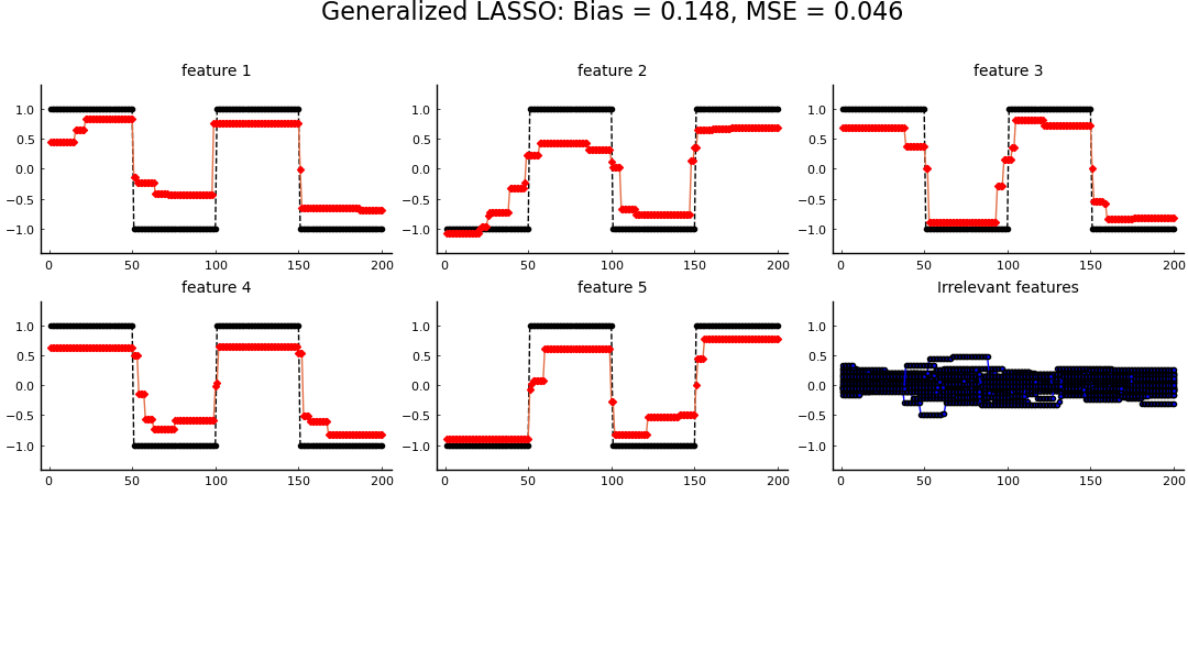
Figure 2: GenLASSO solution example

Table 1: Iterative Fused LASSO

	$n/R=30$	$n/R=50$
$q$\$p$	20 30 40	20 30 40
Panel (a): Bias
2 5 10	0.07 0.08 0.09 0.20 0.24 0.27 0.54 0.49 0.45	0.04 0.03 0.04 0.08 0.07 0.08 0.22 0.34 0.38
Panel (b): MSE
2 5 10	0.02 0.02 0.02 0.12 0.15 0.17 0.51 0.43 0.37	0.01 0.01 0.01 0.03 0.02 0.03 0.16 0.27 0.29

Table 2: Generalized LASSO

	$n/R=30$	$n/R=50$
$q$\$p$	20 30 40	20 30 40
Panel (a): Bias
2 5 10	0.13 0.11 0.10 0.22 0.20 0.20 0.37 0.35 0.35	0.12 0.10 0.09 0.17 0.14 0.14 0.27 0.24 0.23
Panel (b): MSE
2 5 10	0.04 0.03 0.02 0.10 0.09 0.08 0.25 0.23 0.23	0.03 0.02 0.02 0.06 0.05 0.04 0.14 0.12 0.11

Figure 3: Distribution of the bias of the Iterative Fused Lasso, Generalized LASSO and Oracle estimators for the parameters over 100 Monte Carlo replications. Different combinations of candidate and relevant variables. The sample size equals 120 observations.

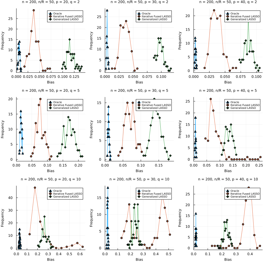
Figure 4: Distribution of the bias of the Iterative Fused Lasso, Generalized LASSO and Oracle estimators for the parameters over 100 Monte Carlo replications. Different combinations of candidate and relevant variables. The sample size equals 200 observations.

7.2 Real-World Dataset results

For the "real-world" dataset, we created a portfolio using $20$ series of daily stock returns ($p=20$), where $3$ relevant (non-zero) features ($q=3$) were active at certain points, resulting in $2$ regimes and $4$ structural breaks. Each regime comprised $758$ observations, spanning from January 2, 2021, to December 23, 2023. To construct this portfolio of returns, we utilized quotes from B3 (Brasil Bolsa Balcao), Brazil’s main hub for trading equities, derivatives, and other financial instruments. The mix of relevant stocks in the portfolio was altered at a single point in time. Initially, the portfolio comprised $25\%$ of stocks from $VALE3$, $25\%$ of stocks from $PETR4$, and $50\%$ of stocks from $ELET6$. After the change, the portfolio shifted to $75\%$ of stocks from $VALE3$, $0\%$ of stocks from $PETR4$, and $25\%$ of stocks from $ELET6$. All other quotes remained non-relevant to the portfolio; however, their returns influenced the observed data in the sense that we observed the portfolio returns.

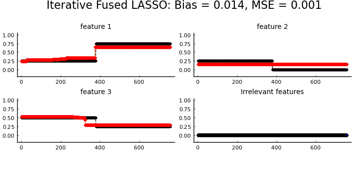
Figure 5: IFL: portfolio dataset

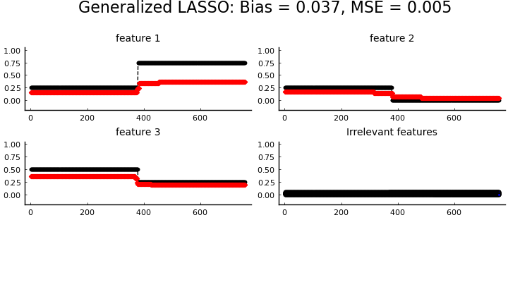
Figure 6: GenLasso: portfolio dataset

Figures 6 and 6 illustrate the estimated feature values over time for each algorithm, respectively. When applied to noisy real data from stock returns, neither algorithm was able to perfectly track every feature value. However, both algorithms achieved relatively small bias and MSE values.

8 Conclusion

Our proposed methodology effectively addresses the challenges of variable selection and structural break detection in high-dimensional time series analysis. The integration of regularization techniques like Fused LASSO and AdaLASSO, coupled with our efficient algorithm, demonstrates superior performance in both simulated and real-world scenarios. In all replications of our Monte Carlo experiments the IFL algorithm was able to correctly identify structural breaks, accurately detect breakpoints, and correctly select variables. This work not only advances the state of high-dimensional time series modeling but also provides a robust framework with practical applicability, paving the way for its adoption in diverse domains requiring sophisticated analytical tools.

References

- [1] Arnold, T.B., Tibshirani, R.J.: genlasso: Path Algorithm for Generalized Lasso Problems (2022), https://CRAN.R-project.org/package=genlasso, r package version 1.6.1
- [2] Breaux, H.J.: On stepwise multiple linear regression. Technical report, Army Ballistic Research Lab, Aberdeen Proving Ground, MD (1967)
- [3] Chow, G.C.: Tests of equality between sets of coefficients in two linear regressions. Econometrica 28(3), 591–605 (1960)
- [4] Epprecht, C.D., Guegan, D., Veiga, ., da Rosa, J.C.: Variable selection and forecasting via automated methods for linear models: Lasso/adalasso and autometrics. Communications in Statistics - Simulation and Computation 50(1), 103–122 (2021). https://doi.org/10.1080/03610918.2018.1554104
- [5] Hoerl, A.E., Kennard, R.W.: Ridge regression: Biased estimation for nonorthogonal problems. Technometrics 12(1), 55–67 (1970)
- [6] Perron, P.: The great crash, the oil price shock, and the unit root hypothesis. Econometrica 57(6), 1361–1401 (1989)
- [7] Tibshirani, R.: Regression shrinkage and selection via the lasso. Journal of the Royal Statistical Society: Series B (Methodological) 58(1), 267–288 (1996), https://www.jstor.org/stable/2346178
- [8] Tibshirani, R., Saunders, M., Rosset, S., Zhu, J., Knight, K.: Sparsity and smoothness via the fused lasso. Journal of the Royal Statistical Society: Series B (Statistical Methodology) 67(1), 91–108 (2005). https://doi.org/10.1111/j.1467-9868.2005.00490.x
- [9] Tibshirani, R.J., Taylor, J.: The solution path of the generalized lasso. Preprint, Stanford University (2011), DOI: 10.1214/11-AOS878, supported by NSF VIGRE fellowship and NSF grants DMS-0852227, DMS-0906801
- [10] Zou, H.: The adaptive lasso and its oracle properties. Journal of the American Statistical Association 101(476), 1418–1429 (2006). https://doi.org/10.1198/016214506000000735