Theoretical and Experimental Constraints on $\mathbb{Z}_{2n}$ Multi-Component Dark Matter Models

Abstract

We investigate extensions of the Standard Model (SM) featuring two-component scalar dark matter (DM) stabilized by a $\mathbb{Z}_{2n}$ symmetry. We focus on three specific cases, $\mathbb{Z}_{4}$, $\mathbb{Z}_{6}(23)$, and $\mathbb{Z}_{6}(13)$, each with a complex and a real scalar singlet. Through detailed numerical scans, we explore the viable parameter space, imposing constraints from DM relic abundance (Planck), direct detection (XENON1T, LZ, PandaX-4T), vacuum stability, perturbative unitarity, and coupling perturbativity up to the GUT and Planck scales, using one-loop renormalization group equations (RGEs). Our results demonstrate that these $\mathbb{Z}_{2n}$ models can provide viable two-component DM scenarios, consistent with all imposed constraints, for a range of DM masses and couplings. We identify the key parameters controlling the DM phenomenology and highlight the importance of a combined analysis incorporating both theoretical and experimental bounds.

1 Introduction

The nature of dark matter remains one of the greatest mysteries in modern physics. Observational evidence, including galaxy rotation curves, gravitational lensing, and anisotropies in the Cosmic Microwave Background (CMB), strongly supports the presence of a non-luminous, non-baryonic component comprising approximately $27\%$ of the universe’s energy density [1, 2, 3, 4, 5]. However, the Standard Model (SM), despite its success in describing fundamental particles and their interactions (excluding gravity), lacks a viable dark matter candidate. This shortcoming extends beyond dark matter, as the SM also fails to explain the origin of neutrino masses [6, 7, 8], the baryon asymmetry of the universe [9, 10], and the strong CP problem [11, 12]. Additionally, precise measurements of the Higgs boson and top quark masses suggest that the SM vacuum lies near the boundary between metastability and stability [13, 14]. These unresolved issues highlight the need for physics Beyond the Standard Model (BSM), particularly in understanding the nature of dark matter.

Extensions of the SM provide promising solutions to its limitations, with notable examples including supersymmetry (SUSY) [15, 16, 17], 331 models [18, 19, 20, 21], and additional gauge symmetries [22, 23, 24]. These models introduce viable dark matter candidates while aligning with observational constraints and future detection prospects.

SUSY predicts superpartners, such as the neutralino, a stable dark matter candidate with a suitable relic abundance [16, 25, 26]. In 331 models with right-handed neutrinos, dark matter can take the form of axions, which also address the strong CP problem. Through nonthermal mechanisms, these axions can account for the total dark matter relic density [27, 28, 29]. Additionally, in a 331 model with a heavy neutral fermion and a WIMP complex scalar, LHC measurements and direct detection data have ruled out the light dark matter window [30]. A natural extension of these frameworks is the scale-invariant 3-3-1-1 model, which incorporates a universal seesaw mechanism for all fermion masses. In this scenario, a discrete matter parity stabilizes a fermionic WIMP that satisfies relic density constraints and remains viable under current direct detection bounds [31].

Additional gauge symmetries, such as $\mathrm{U}(1)_{X}$ and $\mathrm{SU}(2)_{X}$, give rise to new dark matter candidates. In $\mathrm{U}(1)_{X}$ scenarios, Majorana fermions or scalar fields emerge from spontaneous breaking of a hidden $\mathrm{U}(1)_{X}$ symmetry or freeze-in production [32, 33, 34]. Similarly, $\mathrm{SU}(2)_{X}$ models introduce dark gauge bosons and scalar fields, often interacting with the SM via the Higgs portal. These models can support multi-component dark matter and contribute to explaining baryon asymmetry [35, 36, 37].

Simpler SM extensions can also provide viable dark matter candidates, with the inclusion of a scalar singlet being the most straightforward example [38, 39, 40]. A real scalar singlet $S$, stabilized by a discrete $\mathbb{Z}_{2}$ symmetry ($S\to-S$), can act as a dark matter particle near the electroweak scale. This minimal extension maintains simplicity while achieving the observed dark matter abundance through self-annihilation. Despite its appeal, much of the model’s parameter space is excluded by direct detection and relic density constraints. The dark matter mass ($M_{S}$) is viable in two regions: the resonance region around $M_{S}\sim M_{h}/2$, where $M_{h}$ is the Higgs boson mass, requiring very small couplings ($\lambda_{HS}<10^{-2}$), and the high-mass region ($M_{S}\gtrsim 1\,\text{TeV}$), which demands large couplings ($\lambda_{HS}\gtrsim 1$) [41, 42, 43].

To overcome these limitations, multi-component dark matter models, where two or more distinct particles contribute to the total dark matter density, offer a compelling alternative [44, 45, 46, 47, 48, 49, 50, 51]. These models provide greater flexibility in mass ranges, richer phenomenology through diverse interaction mechanisms, and better alignment with current experimental constraints. Additionally, they often yield testable predictions, making them a promising focus for ongoing and future dark matter searches.

Among multi-component dark matter models, those stabilized by a unique $\mathbb{Z}_{N}$ symmetry stand out for their simplicity and theoretical appeal [52, 53, 54, 55, 56]. In these models, $k$ complex scalar fields act as dark matter components, each being an SM singlet with a distinct charge under $\mathbb{Z}_{N}$, satisfying $N\geq 2k$. Notably, this symmetry can emerge as a discrete gauge symmetry from the spontaneous breaking of a $\mathrm{U}(1)_{X}$ gauge group, where the associated scalar carries an $X$-charge of $N$ [57, 58], establishing a direct connection to gauge extensions of the SM. A well-known example in the two-component case ($k=2$) is the $\mathbb{Z}_{5}$ model [59], which accommodates dark matter masses below the TeV scale while remaining consistent with current experimental bounds. Additionally, it predicts that both dark matter particles could produce detectable signals in current and future direct detection experiments.

A particularly interesting class of these models arises when $N=2n$ is even, featuring a complex field ($S_{A}$) and a real one ($S_{B}$). In such $\mathbb{Z}_{2n}$ scenarios, the real scalar transforms as $S_{B}\to-S_{B}$ under the symmetry. Ref. [56] investigated cases with $N=4$ and $N=6$, where the latter allows two distinct charge assignments, leading to the $\mathbb{Z}_{6}(23)$ and $\mathbb{Z}_{6}(13)$ models. Their analysis highlighted the critical role of semi-annihilation processes mediated by trilinear interactions. The findings indicate that the $\mathbb{Z}_{4}$ and $\mathbb{Z}_{6}(23)$ scenarios remain viable across a broad range of dark matter masses ($M\lesssim 2$ TeV) and could be tested in upcoming direct detection experiments. Conversely, the $\mathbb{Z}_{6}(13)$ scenario faces stringent constraints due to the absence of semi-annihilation channels and the inefficiency of dark matter conversion processes in sufficiently reducing the relic abundance of the lightest dark matter particle.

Unlike minimal scalar dark matter models, the presence of multiple interactions between the dark and visible sectors can significantly affect the stability of the scalar potential and the validity of the theory at high energies. Ensuring both quantum stability and perturbative unitarity is a fundamental challenge in BSM theories, as the interplay between these constraints often restricts the viable parameter space. A rigorous theoretical and phenomenological analysis is therefore essential to assess model viability, comply with experimental bounds, and guide the search for new physics by delineating consistent theoretical frameworks.

Given these theoretical constraints, it is essential to develop systematic methods for assessing the stability of scalar potentials in BSM scenarios. In such extensions of the SM, additional scalar fields and interactions introduce a greater number of quartic terms, making the derivation of stability conditions increasingly complex. A powerful tool for addressing this challenge is the orbit space method [60, 61, 62], which simplifies the analysis by focusing on field magnitude squares and orbit parameters, effectively reducing the number of independent variables. Additionally, discrete symmetries, commonly invoked to stabilize dark matter candidates, can impose structural constraints on the scalar potential. In many cases, these symmetries enforce biquadratic interactions of the form $\lambda_{ij}\phi_{i}^{2}\phi_{j}^{2}$, allowing stability analysis to be reformulated in terms of the copositivity of the coupling matrix $\lambda_{ij}$ [63, 64, 65, 66]. These classical stability conditions provide a crucial foundation for evaluating the viability of BSM theories.

Quantum corrections play a crucial role in determining the stability of the scalar potential, making the use of the effective potential essential. One-loop corrections introduce logarithmic terms that depend on the mass eigenvalues and the renormalization group scale. In multiscale effective potentials, where mass eigenvalues differ significantly, choosing a single renormalization scale that maintains perturbative control over these corrections becomes impractical. This challenge underscores the need for advanced methods to accurately assess quantum stability.

Several methods have been proposed to improve the multi-scale effective potential [67, 68, 69, 70], often by introducing multiple renormalization scales and requiring partial renormalization group equations. A promising approach is to solve the renormalization group equation with a boundary condition on a hypersurface where quantum corrections vanish [71]. Using a single, field-dependent renormalization scale in this framework extends the perturbative validity range, limited to $\lambda_{i}<4\pi$, and allows tree-level stability criteria to be applied to the improved effective potential. This method simplifies the analysis by replacing classical quartic couplings with their running counterparts from Renormalization Group Equations (RGEs), enabling a more robust evaluation of vacuum stability under quantum corrections and bridging the gap between classical and quantum analyses.

While quantum stability constrains the scalar potential at high energies, perturbative unitarity provides an independent yet complementary criterion for theoretical consistency. A pioneering result in Ref. [72, 73] showed that perturbative unitarity imposes an upper limit of approximately 1 TeV on the SM Higgs boson mass. This finding not only constrained the Higgs sector but also established a key framework for bounding scalar couplings in BSM theories, where additional parameters are often weakly constrained by experiments. Maintaining perturbative unitarity in high-energy scattering processes is essential for theoretical consistency in quantum field theory. Derived from tree-level two-body scattering amplitudes, these constraints ensure the unitarity of the S-matrix, a fundamental principle of quantum mechanics. In practice, they impose strict upper bounds on coupling constants and scalar masses, working alongside stability conditions to refine the viable parameter space. As such, they are crucial for understanding SM extensions and guiding future directions in particle physics.

Although $\mathbb{Z}_{2n}$ multi-component dark matter models have been explored phenomenologically, comprehensive theoretical analyses of the constraints imposed by quantum vacuum stability and unitarity remain scarce. In this work, we integrate a study of the classical stability of the scalar potential with a detailed quantum analysis based on the improved multi-scale effective potential, providing a more robust assessment of vacuum stability under radiative corrections. Furthermore, we impose unitarity constraints on the scalar couplings to ensure the theoretical consistency of the models at high energy scales. This approach refines the parameter space, identifying viable regions and establishing direct connections to experimental observables.

To structure our analysis, we begin in Section 2 with a general review of the $\mathbb{Z}_{2n}$ models, highlighting their symmetric properties and scalar sectors. Section 3 discusses the classical stability conditions of the scalar potential and extends the analysis to the quantum level using a renormalized effective potential to account for radiative corrections. In Section 4, we examine unitarity constraints and their impact on model viability. Section 5 explores dark matter phenomenology, focusing on relic abundance constraints and direct detection prospects. In Section 6, we present a comprehensive discussion of our findings and their implications for future experimental and theoretical studies. Finally, Section 7 summarizes our conclusions. Appendix A provides the Renormalization Group Equations necessary for analyzing the quantum vacuum stability.

2 The Generalities of the $\mathbb{Z}_{2n}$ Models

The models under consideration extend the SM by incorporating a discrete $\mathbb{Z}_{2n}$ symmetry. In this framework, the scalar sector consists of a complex scalar field, $S_{A}$, and a real scalar field, $S_{B}$. The real scalar transforms under $\mathbb{Z}_{2n}$ symmetry as $S_{B}\to-S_{B}$, ensuring stability.

The most general Lagrangian for the $\mathbb{Z}_{2n}$ models can be expressed as:

$$\mathcal{L}=\mathcal{L}_{\text{SM}}+\mathcal{L}_{\text{DM}},$$ (2.1)

where $\mathcal{L}_{\text{SM}}$ represents the SM sector, including $V_{\text{SM}}=-\mu_{H}^{2}|H|^{2}+\lambda_{H}|H|^{4}$. The second term, $\mathcal{L}_{\text{DM}}$, represents the dark sector contribution and is given by:

$$\mathcal{L}_{\text{DM}}=(\partial_{\mu}S_{A}^{*})(\partial^{\mu}S_{A})+\frac{1}{2}(\partial_{\mu}S_{B})(\partial^{\mu}S_{B})-V(H,S_{A},S_{B}),$$ (2.2)

where the scalar potential associated with the extended sector is $V(H,S_{A},S_{B})=V_{\text{DM}}+V_{\text{int}}$, with each term expressed as:

$$V_{\text{DM}} =-\mu_{A}^{2}|S_{A}|^{2}+\lambda_{A}|S_{A}|^{4}-\frac{1}{2}\mu_{B}^{2}S_{B}^{2}+\lambda_{B}S_{B}^{4},$$ (2.3)

$$V_{\text{int}} =\lambda_{HA}|H|^{2}|S_{A}|^{2}+\frac{1}{2}\lambda_{HB}|H|^{2}S_{B}^{2}+\lambda_{AB}|S_{A}|^{2}S_{B}^{2}.$$ (2.4)

After electroweak symmetry breaking (EWSB), the Higgs acquires a vacuum expectation value, $\langle H\rangle=\frac{1}{\sqrt{2}}(0,\,v)^{\text{T}}$, leading to mass terms for the scalars:

$$M_{h}^{2}=2\lambda_{H}v^{2},\quad M_{S_{A}}^{2}=\frac{1}{2}\lambda_{HA}v^{2}-\mu_{A}^{2},\quad M_{S_{B}}^{2}=\frac{1}{2}\lambda_{HB}v^{2}-\mu_{B}^{2}.$$ (2.5)

Beyond the general structure described above, the $\mathbb{Z}_{4}$ and $\mathbb{Z}_{6}$ models include additional terms, as summarized in Table 1. In the $\mathbb{Z}_{6}$ model, two distinct charge assignments are possible, giving rise to two scenarios, denoted as $\mathbb{Z}_{6}(23)$ and $\mathbb{Z}_{6}(13)$. The terms in Table 1 introduce crucial phenomenological differences between these models. The $\mathbb{Z}_{4}$ model allows for trilinear and quartic interactions that influence both dark matter phenomenology and the vacuum structure. In contrast, the $\mathbb{Z}_{6}(23)$ model features a cubic interaction that affects dark matter annihilation channels, while the $\mathbb{Z}_{6}(13)$ model contains only quartic interactions.

Table 1: Additional scalar potential terms for the $\mathbb{Z}_{4}$ and $\mathbb{Z}_{6}$ models. Here, $\omega_{n}=e^{i2\pi/n}$ represents the $n^{\text{th}}$ root of unity.

Model	Additional Scalar Potential Terms	Charge Assignments
$\mathbb{Z}_{4}$	$\frac{1}{2}(\mu_{S1}S_{A}^{2}S_{B}+\lambda_{S4}S_{A}^{4})+$ h.c.	$S_{A}\to\omega_{4}S_{A},\quad S_{B}\to\omega_{4}^{2}S_{B}$
$\mathbb{Z}_{6}(23)$	$\frac{1}{3}\mu_{S2}S_{A}^{3}+$ h.c.	$S_{A}\to\omega_{6}^{2}S_{A},\quad S_{B}\to\omega_{6}^{3}S_{B}$
$\mathbb{Z}_{6}(13)$	$\frac{1}{3}\lambda^{\prime}_{AB}S_{A}^{3}S_{B}+$ h.c.	$S_{A}\to\omega_{6}S_{A},\quad S_{B}\to\omega_{6}^{3}S_{B}$

3 Classical and Quantum Vacuum Stability

For a scalar potential to be physically acceptable, it must be bounded from below; otherwise, the theory becomes unstable due to the absence of a lowest energy state. At tree level, the potential is a polynomial in the scalar fields and is bounded from below if it remains positive in the large-field limit along any direction in field space. In this regime, the quartic term, $V_{4}$, dominates over lower-degree terms, allowing mass and cubic contributions to be neglected in vacuum stability calculations. The condition $V_{4}>0$ ensures strong stability, while $V_{4}\geq 0$ corresponds to marginal stability, which excludes cubic terms.

In SM extensions, additional scalars introduce more quartic terms, complicating stability conditions. While general analytical criteria remain elusive, recent progress has been made [74]. Explicit conditions exist for specific cases, such as two real scalar fields, potentials including the Higgs, and the two-Higgs-doublet model without explicit CP violation [75].

In this section, we first examine the classical stability conditions of the scalar potential, employing methods such as the orbit space approach and the copositivity of the quartic coupling matrix. We then extend the analysis to the quantum level at order $\hbar$, adopting the method proposed in [71]. This approach improves the effective potential by introducing a single, field-dependent renormalization scale, enabling the use of the same stability conditions with renormalization-group-improved quartic couplings.

3.1 Classical Vacuum Stability

We employ the orbit space method to systematically derive vacuum stability conditions in the $\mathbb{Z}_{2n}$ models discussed in the previous section. This powerful approach reformulates the potential in terms of field magnitude squares, $|\phi|^{2}\equiv\phi_{k}^{*}\phi_{k}$, and dimensionless orbit parameters, $\theta\equiv\frac{f_{ijkl}\phi_{i}^{*}\phi_{j}\phi_{k}^{*}\phi_{l}}{|\phi|^{4}}$, simplifying the analysis. It applies even to fields in higher multiplets under a gauge group, reducing complexity by focusing on symmetries and transformations. This makes it a valuable technique for studying vacuum stability in extended models [75, 60, 61]. In the $\mathbb{Z}_{4}$ and $\mathbb{Z}_{6}(23)$ models, the quartic part of the scalar potential takes the form of a biquadratic expression, $\lambda_{ij}\phi_{i}^{2}\phi_{j}^{2}$, involving squared real fields or the squared norms of complex fields. This structure naturally arises due to the discrete symmetry that stabilizes dark matter, restricting terms that could lead to its destabilization. In these cases, the quartic potential can be written as $V_{4}=\mathbf{h}^{\text{T}}\Lambda\mathbf{h}$, where $\Lambda$ is a symmetric $N_{\phi}\times N_{\phi}$ matrix and $\mathbf{h}$ is a vector with non-negative components in the basis $\{\phi_{1}^{2},\dots,\phi_{N_{\phi}}^{2}\}$. The potential is bounded from below if $\Lambda$ is copositive [66], or strictly copositive for strong stability. General copositivity conditions for symmetric matrices can be found in [63, 65].

To analyze vacuum stability in these models, we focus on the specific case of a symmetric $3\times 3$ matrix, $\mathrm{A}_{3\times 3}$, under strong stability conditions ($V_{4}>0$), which require:

$$\begin{split}&\hskip 108.405pta_{11}>0,\quad a_{22}>0,\quad a_{33}>0,\\ &\bar{a}_{12}\equiv a_{12}+\sqrt{a_{11}a_{22}}>0\ ,\quad\bar{a}_{13}\equiv a_{13}+\sqrt{a_{11}a_{33}}>0,\quad\bar{a}_{23}\equiv a_{23}+\sqrt{a_{22}a_{33}}>0,\\ &\hskip 43.36464pta_{12}\sqrt{a_{33}}+a_{13}\sqrt{a_{22}}+a_{23}\sqrt{a_{11}}+\sqrt{a_{11}a_{22}a_{33}}+\sqrt{2\bar{a}_{12}\bar{a}_{13}\bar{a}_{23}}>0,\end{split}$$ (3.1)

where $a_{ij}$ is an element of $\mathrm{A}_{3\times 3}$.

For the $\mathbb{Z}_{6}(13)$ model, the quartic potential does not have this biquadratic structure due to the presence of the $\lambda^{\prime}_{AB}$ term. Therefore, the copositivity method, as described above, is not directly applicable. We address this case using an alternative approach, detailed below. We first present the vacuum stability conditions for the $\mathbb{Z}_{4}$ and $\mathbb{Z}_{6}(23)$ models, where the copositivity approach is directly applicable.

3.2 $\mathbb{Z}_{4}$ model

The quartic part of the $\mathbb{Z}_{4}$ model scalar potential which is

$$V_{4}=\lambda_{H}|H|^{4}+\lambda_{A}|S_{A}|^{4}+\lambda_{B}S_{B}^{4}+\lambda_{AB}|S_{A}|^{2}S_{B}^{2}+\lambda_{HA}|H|^{2}|S_{A}|^{2}+\frac{1}{2}\lambda_{HB}|H|^{2}S_{B}^{2}+\frac{1}{2}\lambda_{S4}\theta|S_{A}|^{4},$$ (3.2)

can be written as $V_{4}\equiv\mathbf{h}^{\text{T}}\Lambda\mathbf{h}>0$ where $\mathbf{h}^{\text{T}}=(|H|^{2},|S_{A}|^{2},S_{B}^{2})\geq 0$ and, the symmetric $3\times 3$ matrix $\Lambda$ is

$$\Lambda=\begin{pmatrix}\lambda_{H}&\frac{\lambda_{HA}}{2}&\frac{\lambda_{HB}}{4}\\ *&\lambda_{A}+\frac{1}{2}\lambda_{S4}\theta&\frac{\lambda_{AB}}{2}\\ *&*&\lambda_{B}\end{pmatrix}.$$ (3.3)

The quartic term follows a biquadratic form in the field norms. Due to the presence of the cubic term $\frac{1}{2}\mu_{S1}S_{A}^{2}S_{B}$, we impose the strong stability condition ($V_{4}>0$), allowing the use of strict copositivity. The orbit parameter $\theta$ is defined as

$$\theta=\hat{S}_{A}^{4}+(\hat{S}_{A}^{*})^{4},$$ (3.4)

where $\hat{S}_{A}\equiv S_{A}/|S_{A}|$. Expressing $S_{A}=re^{i\alpha}$, we obtain

$$\theta=2\cos(4\alpha)\implies-2\leq\theta\leq 2.$$ (3.5)

The potential is bounded from below if $\Lambda$ is strictly copositive for all $\theta\in[-2,2]$. If $V_{4}<0$ for some $\theta$ with $|\mathbf{h}|=1$, the vacuum is unstable. Conversely, if $V_{4}>0$ at the $\theta$ that minimizes $V_{4}$ for $|\mathbf{h}|=1$, the potential remains bounded for all $\theta$. Since $V_{4}$ is monotonic in $\theta$, the extrema occur at $\theta=\pm 2$. The minimum is at $\theta=-2$ for $\lambda_{S4}\geq 0$ and at $\theta=2$ for $\lambda_{S4}<0$. Applying the copositivity conditions from Eq. (3.1) to $\Lambda$ in Eq. (3.3), with $\theta$ evaluated at these boundaries, we obtain the vacuum stability conditions for the $\mathbb{Z}_{4}$ model:

$$\begin{split}&\hskip 32.52017pt\lambda_{H}>0,\quad\lambda_{A}-|\lambda_{S4}|>0,\quad\lambda_{B}>0,\quad C_{1}\equiv\lambda_{AB}+2\sqrt{(\lambda_{A}-|\lambda_{S4}|)\lambda_{B}}>0,\\ &\hskip 47.69846ptC_{2}\equiv\lambda_{HA}+2\sqrt{\lambda_{H}(\lambda_{A}-|\lambda_{S4}|)}>0,\quad C_{3}\equiv\lambda_{HB}+4\sqrt{\lambda_{H}\lambda_{B}}>0,\\ &2\lambda_{AB}\sqrt{\lambda_{H}}+2\lambda_{HA}\sqrt{\lambda_{B}}+\lambda_{HB}\sqrt{\lambda_{A}-|\lambda_{S4}|}+4\sqrt{\lambda_{H}(\lambda_{A}-|\lambda_{S4}|)\lambda_{B}}+\sqrt{2C_{1}C_{2}C_{3}}>0.\end{split}$$ (3.6)

3.3 $\mathbb{Z}_{6}(23)$ model

The quartic part of the $\mathbb{Z}_{6}(23)$ scalar potential is

$$V_{4}=\lambda_{H}|H|^{4}+\lambda_{A}|S_{A}|^{4}+\lambda_{B}S_{B}^{4}+\lambda_{AB}|S_{A}|^{2}S_{B}^{2}+\lambda_{HA}|H|^{2}|S_{A}|^{2}+\frac{1}{2}\lambda_{HB}|H|^{2}S_{B}^{2}.$$ (3.7)

It can be rewritten as $V_{4}=\mathbf{h}^{\text{T}}\Lambda\mathbf{h}>0$, where $\mathbf{h}^{\text{T}}=(|H|^{2},|S_{A}|^{2},S_{B}^{2})\geq 0$, and the symmetric $3\times 3$ matrix $\Lambda$ is

$$\Lambda=\begin{pmatrix}\lambda_{H}&\frac{\lambda_{HA}}{2}&\frac{\lambda_{HB}}{4}\\ *&\lambda_{A}&\frac{\lambda_{AB}}{2}\\ *&*&\lambda_{B}\end{pmatrix}.$$ (3.8)

As in the $\mathbb{Z}_{4}$ model, strict copositivity applies to $\mathbb{Z}_{6}(23)$ since $V_{4}$ is biquadratic in the field norms and includes the cubic term $\frac{1}{3}\mu_{S2}S_{A}^{3}$. With no orbit parameters in this case, we directly apply the copositivity conditions from Eq. (3.1) to $\Lambda$ in Eq. (3.8). The vacuum stability conditions for the $\mathbb{Z}_{6}(23)$ model are

$$\begin{split}&\hskip 26.01613pt\lambda_{H}>0,\quad\lambda_{A}>0,\quad\lambda_{B}>0,\quad C_{1}\equiv\lambda_{AB}+2\sqrt{\lambda_{A}\lambda_{B}}>0,\\ &\hskip 29.27145ptC_{2}\equiv\lambda_{HA}+2\sqrt{\lambda_{H}\lambda_{A}}>0,\quad C_{3}\equiv\lambda_{HB}+4\sqrt{\lambda_{H}\lambda_{B}}>0,\\ &2\lambda_{AB}\sqrt{\lambda_{H}}+2\lambda_{HA}\sqrt{\lambda_{B}}+\lambda_{HB}\sqrt{\lambda_{A}}+4\sqrt{\lambda_{H}\lambda_{A}\lambda_{B}}+\sqrt{2C_{1}C_{2}C_{3}}>0.\end{split}$$ (3.9)

Notably, these stability conditions match those of the $\mathbb{Z}_{4}$ model when $\lambda_{S4}=0$.

3.4 $\mathbb{Z}_{6}(13)$ model

The quartic part of the $\mathbb{Z}_{6}(13)$ scalar potential is

$$V_{4}=\lambda_{H}|H|^{4}+\lambda_{A}|S_{A}|^{4}+\lambda_{B}S_{B}^{4}+\lambda_{AB}|S_{A}|^{2}S_{B}^{2}+\lambda_{HA}|H|^{2}|S_{A}|^{2}+\frac{1}{2}\lambda_{HB}|H|^{2}S_{B}^{2}+\frac{1}{3}\lambda_{AB}^{\prime}\theta^{\prime}|S_{A}|^{3}S_{B}.$$ (3.10)

The orbit parameter $\theta^{\prime}$ is defined as

$$\theta^{\prime}=\hat{S}_{A}^{3}+(\hat{S}_{A}^{*})^{3},$$ (3.11)

where $\hat{S}_{A}\equiv S_{A}/|S_{A}|$. Following a calculation analogous to that for $\theta$ in Eq. (3.5), we find $\theta^{\prime}\in[-2,2]$.

For $\lambda_{AB}^{\prime}=0$, the stability conditions of $\mathbb{Z}_{6}(13)$ reduce to those of $\mathbb{Z}_{6}(23)$ under strong stability ($V_{4}>0$). However, when $\lambda_{AB}^{\prime}\neq 0$, copositivity does not apply, requiring an alternative approach. We use the vacuum stability conditions from [75] for a general scalar potential with two real scalar fields and one Higgs doublet, mapping them to the $\mathbb{Z}_{6}(13)$ model. The conditions, given in Eq. (61) of Section 4 of [75], are expressed as functions of the quartic couplings

$$\mathrm{StabCondV12H}\left[\lambda_{40},\lambda_{31},\lambda_{22},\lambda_{13},\lambda_{04},\lambda_{H},\lambda_{H20},\lambda_{H11},\lambda_{H02}\right],$$ (3.12)

where the couplings in Eq. (3.12) are defined in the potential $V(\phi_{1},\phi_{2},|H|^{2})$, given in Eq. (42) of [75]. Comparing $V(\phi_{1},\phi_{2},|H|^{2})$ with $V_{4}$ in Eq. (3.10), we establish the mapping:

$$\mathrm{StabCondV12H}\left[\lambda_{A},\frac{1}{3}\lambda_{AB}^{\prime}\theta^{\prime},\lambda_{AB},0,\lambda_{B},\lambda_{H},\lambda_{HA},0,\frac{1}{2}\lambda_{HB}\right].$$ (3.13)

To determine the vacuum stability conditions, we evaluate $\theta^{\prime}$ at its extrema, $\theta^{\prime}=\pm 2$, following the same procedure as in the $\mathbb{Z}_{4}$ model. However, in this case, both the sign of $\lambda_{AB}^{\prime}$ and that of $S_{B}$ must be considered. The final stability conditions for the $\mathbb{Z}_{6}(13)$ model are

$$\begin{split}&\mathrm{StabCondV12H}\left[\lambda_{A},\frac{2}{3}|\lambda_{AB}^{\prime}|,\lambda_{AB},0,\lambda_{B},\lambda_{H},\lambda_{HA},0,\frac{1}{2}\lambda_{HB}\right],\\ &\mathrm{StabCondV12H}\left[\lambda_{A},-\frac{2}{3}|\lambda_{AB}^{\prime}|,\lambda_{AB},0,\lambda_{B},\lambda_{H},\lambda_{HA},0,\frac{1}{2}\lambda_{HB}\right].\end{split}$$ (3.14)

Both conditions must be satisfied simultaneously.

3.5 Quantum Vacuum Stability

We now focus on quantum-level stability, where corrections modify the classical conditions, requiring the use of the effective potential. At one-loop level, it is given by

$$V_{\text{Eff}}(\mu,\lambda,\phi)=\overbrace{V^{(0)}(\lambda,\phi)}^{\text{Tree level}}\,+\,\overbrace{\frac{\hbar}{64\pi^{2}}\sum_{a}n_{a}m_{a}^{4}(\lambda,\phi)\left[\ln\frac{m_{a}^{2}(\lambda,\phi)}{\mu^{2}}-\chi_{a}\right]}^{\text{One-loop correction (Coleman-Weinberg)}}+\,\mathcal{O}\left(\hbar^{2}\right).$$ (3.15)

Here, the index $a$ runs over all particle species, with $m_{a}(\lambda,\phi)$ denoting the tree-level, field-dependent mass eigenvalues. The factor $n_{a}$ represents the degrees of freedom for each particle, while $\chi_{a}$ is a constant that depends on the renormalization scheme. The parameters $\lambda$ and $\phi$ collectively denote all couplings and classical scalar fields, respectively, and $\mu$ is the renormalization scale.

For perturbativity in Eq. (3.15), couplings must remain small ($\lambda<4\pi$), and large logarithmic corrections must be avoided. When mass scales differ significantly, no single $\mu$ can keep all logarithms under control, invalidating the perturbative expansion. This issue is common in SM extensions, particularly in $\mathbb{Z}_{2n}$ models, where dark matter masses can deviate substantially from those of SM particles.

To address this, we introduce a field-dependent renormalization scale $\mu^{*}$ [71], defined on a hypersurface where one-loop corrections vanish. This ensures that the effective potential matches the classical potential evaluated at the running couplings $\lambda(\mu^{*})$:

$$V(\mu^{*},\lambda,\phi)=V^{(0)}(\lambda(\mu^{*}),\phi(\mu^{*})).$$ (3.16)

Although no single $\mu$ removes all logarithms, choosing it on the hypersurface minimizes their impact. As a result, the perturbative validity range is significantly extended, constrained only by $\lambda(\mu^{*})<4\pi$.

Another key advantage of this method is that it allows classical stability conditions to be applied to the improved effective potential. By solving the Renormalization Group Equations (RGEs), the tree-level couplings in stability criteria are replaced with their running values, $\lambda(\mu^{*})$. Consequently, stability conditions valid at the electroweak scale may not hold at higher energies, further restricting the parameter space.

To implement this approach, we solve the RGEs numerically. Computing them in SM extensions is challenging due to the large number of Feynman diagrams and parameters, but tools such as SARAH, RGBeta, ARGES, and PyR@TE automate these calculations [76, 77, 78, 79]. To ensure consistency, we crosschecked our RGEs using both SARAH and RGBeta. A one-loop calculation is sufficient to capture the key quantum effects, and the corresponding RGEs are listed in Appendix A.

4 Perturbative Unitarity

In this section, we derive perturbative unitarity constraints for all models considered in this work by analyzing tree-level two-body scattering amplitudes. This ensures the preservation of S-matrix unitarity, a fundamental requirement in quantum field theory. By examining these amplitudes, we establish conditions that maintain theoretical consistency.

We employ a well-established approach based on high-energy scattering processes involving scalar external states [72, 73, 80, 81, 82]. This method is justified by the Goldstone boson equivalence theorem, which allows replacing external longitudinal gauge bosons with their corresponding Goldstone modes. Consequently, the amplitudes for these scattering processes remain equivalent to those involving longitudinal gauge bosons, up to corrections of order $\mathcal{O}(M_{W}^{2}/s)$, which become negligible in the high-energy limit $s\gg M_{W}^{2}$.

The unitarity constraints are derived directly from the partial wave expansion, leading to the condition [81, 82]

$$-\frac{i}{2}(a_{J}-a_{J}^{\dagger})\geq a_{J}a_{J}^{\dagger}\quad\forall J,$$ (4.1)

where $a_{J}$ is the matrix associated with the partial wave decomposition of the $2\to 2$ scattering amplitudes $a_{J}^{ba}$. These elements are given by

$$a_{J}^{ba}=\frac{1}{32\pi}\sqrt{\frac{4|\mathbf{p}^{b}||\mathbf{p}^{a}|}{2^{\delta_{12}}2^{\delta_{34}}\,s}}\int_{-1}^{1}d(\cos\theta)\mathcal{M}_{ba}(\cos\theta)P_{J}(\cos\theta),$$ (4.2)

where $\mathcal{M}_{ba}(\cos\theta)$ represents the scattering amplitude for an initial state $a=\{1,2\}$ with momenta $p_{1}$ and $p_{2}$ transitioning to a final state $b=\{3,4\}$ with momenta $p_{3}$ and $p_{4}$.

The factors $\delta_{12}$ and $\delta_{34}$ take the value 1 if the corresponding pair of particles is identical and 0 otherwise. The angle $\theta$ is defined as the angle between the incoming three-momentum $\mathbf{p}^{a}$ and the outgoing three-momentum $\mathbf{p}^{b}$ in the center-of-mass frame. The squared center-of-mass energy is given by the Mandelstam variable $s=(p_{1}+p_{2})^{2}$, and $P_{J}(\cos\theta)$ are the Legendre polynomials.

Since the matrix $a_{J}$ is normal, both $a_{J}$ and $a_{J}^{\dagger}$ can be diagonalized using the same unitary matrix. Consequently, the condition (4.1) can be rewritten in terms of the eigenvalues $a_{J}^{i}$ as [80, 81, 82]

$$\operatorname{Im}(a_{J}^{i})\geq|a_{J}^{i}|^{2}\quad\forall J,i.$$ (4.3)

This condition defines a circular region in the complex plane with radius $1/2$, centered at $(\operatorname{Re}a_{J}^{i},\allowbreak\operatorname{Im}a_{J}^{i})=(0,1/2)$. Consequently, the constraint translates into the following conditions that each $a_{J}^{i}$ must satisfy:

$$|a_{J}^{i}|\leq 1,\quad|\operatorname{Re}a_{J}^{i}|\leq\frac{1}{2},\quad 0\leq\operatorname{Im}a_{J}^{i}\leq 1\quad\forall J,i.$$ (4.4)

In the high-energy limit ($s\to\infty$), only quartic interactions contribute to $2\to 2$ scattering processes, as diagrams involving propagators are suppressed and can be neglected. Moreover, it is sufficient to consider only the $J=0$ contribution in the partial wave decomposition. Since $\sqrt{4|\mathbf{p}^{b}||\mathbf{p}^{a}|/s}\to 1$ as $s\to\infty$, the $a_{0}^{ba}$ term simplifies to

$$a_{0}^{ba}=\frac{1}{32\pi}\frac{1}{\sqrt{2^{{\delta}_{12}}2^{{\delta}_{34}}}}\int_{-1}^{1}d(\cos\theta)\,\mathcal{M}_{ba}(\cos\theta).$$ (4.5)

For quartic interactions, the scattering amplitude $\mathcal{M}_{ba}(\cos\theta)$ is given by the negative fourth derivative of the scalar potential $V$ evaluated after electroweak symmetry breaking. Explicitly,

$$a_{0}^{ba}=-\frac{1}{16\pi}\frac{1}{\sqrt{2^{{\delta}_{12}}2^{{\delta}_{34}}}}\frac{\partial^{4}V}{\partial\phi_{1}\partial\phi_{2}\partial\phi_{3}\partial\phi_{4}}.$$ (4.6)

In practical applications, one of the first two unitarity conditions from Eq. (4.4) is typically chosen to constrain the theory. The most commonly used criterion is [80, 83]

$$|\operatorname{Re}a_{0}^{i}\,|\leq\frac{1}{2},\quad\forall i.$$ (4.7)

This condition keeps the theory within the perturbative regime, ensuring unitarity and the reliability of phenomenological predictions. Although widely adopted for its conservative approach, the alternative criterion, $|a_{J}^{i}|\leq 1$, also appears in the literature and reflects a matter of preference [83].

The expression for $a_{0}^{ba}$ in Eq. (4.6), combined with the unitarity condition in Eq. (4.7), establishes the framework for deriving perturbative unitarity constraints for any model under consideration. Based on this, we now present the unitarity bounds for the $\mathbb{Z}_{2n}$ models, using the scalar potential present in Eq. (2.1), along with the additional terms specific to the $\mathbb{Z}_{4}$, $\mathbb{Z}_{6}(23)$, and $\mathbb{Z}_{6}(13)$ models, as summarized in Table 1. The results are organized into general constraints applicable to all models and specific conditions for each individual scenario.

The perturbative unitarity constraints that apply universally to all models are given by

$$\begin{split}&|\lambda_{H}|\leq 4\pi,\quad|\lambda_{HA}|\leq 8\pi,\quad|\lambda_{HB}|\leq 8\pi,\quad|x_{1,2,3}|\leq 16\pi,\end{split}$$ (4.8)

where $x_{1,2,3}$ are the roots of the cubic equation

$$x^{3}+Ax^{2}+Bx+C=0,$$ (4.9)

with coefficients

$$A =12\lambda_{H}+8\lambda_{A}+24\lambda_{B},$$ (4.10)

$$B =96\lambda_{H}\lambda_{A}+288\lambda_{H}\lambda_{B}+192\lambda_{A}\lambda_{B}-8\lambda_{AB}^{2}-8\lambda_{HA}^{2}-4\lambda_{HB}^{2},$$ (4.11)

$$C =2304\lambda_{H}\lambda_{A}\lambda_{B}-96\lambda_{H}\lambda_{AB}^{2}-32\lambda_{A}\lambda_{HB}^{2}-192\lambda_{B}\lambda_{HA}^{2}+32\lambda_{AB}\lambda_{HA}\lambda_{HB}.$$ (4.12)

For the $\mathbb{Z}_{4}$ model, the additional unitarity constraints are

$$\left|\lambda_{A}\pm 3\lambda_{S_{4}}\right|\leq 4\pi,\quad|\lambda_{AB}|\leq 4\pi.$$ (4.13)

For the $\mathbb{Z}_{6}(23)$ model, the remaining unitarity constraints are

$$|\lambda_{A}|\leq 4\pi,\quad|\lambda_{AB}|\leq 4\pi.$$ (4.14)

For the $\mathbb{Z}_{6}(13)$ model, the extra unitarity condition is

$$\left|\lambda_{A}+\lambda_{AB}\pm\sqrt{\left(\lambda_{A}-\lambda_{AB}\right)^{2}+2\lambda_{AB}^{\prime 2}}\right|\leq 8\pi.$$ (4.15)

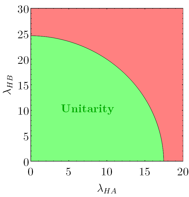
(a) Classical unitarity constraints. The green region represents the parameter space where unitarity is preserved, while the red region indicates its violation. The plot is symmetric under sign changes of $\lambda_{HA}$ and $\lambda_{HB}$.

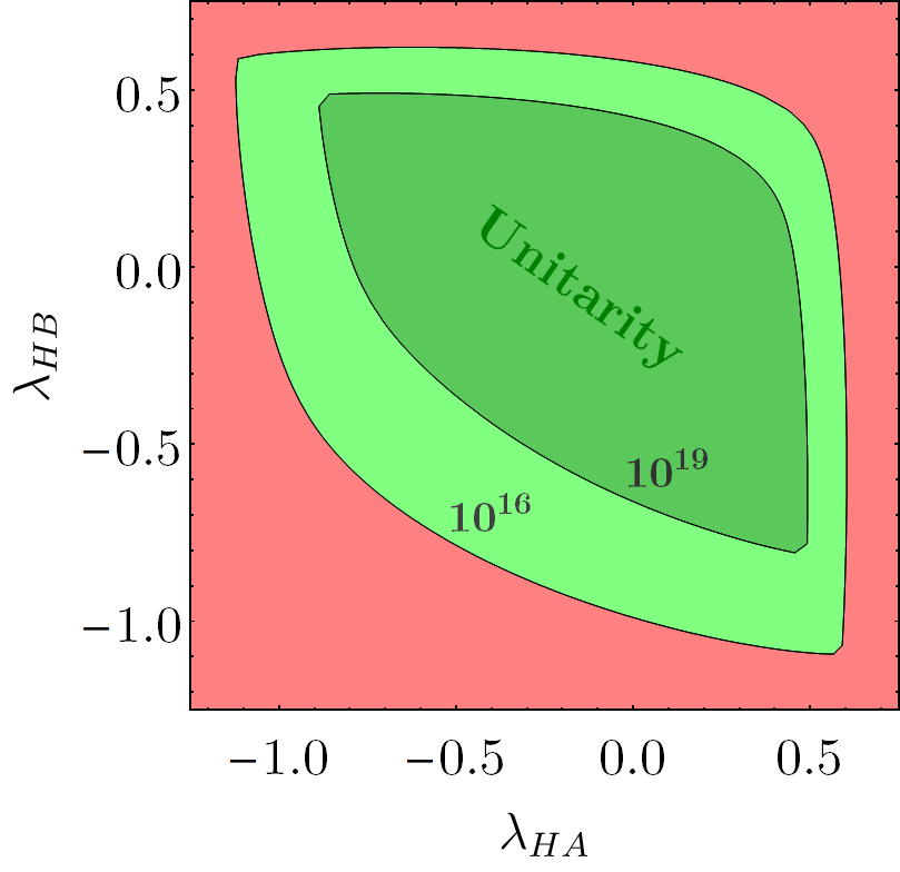
(b) Unitarity constraints with running couplings from the electroweak scale to the GUT and Planck scales at one-loop order. Dark green denotes unitarity up to the Planck scale, light green up to the GUT scale, and red marks unitarity violation. At the quantum level, the symmetry under sign reversal of $\lambda_{HA}$ and $\lambda_{HB}$ is broken.

Figure 1: Unitarity bounds in the $\lambda_{HA}$–$\lambda_{HB}$ plane for the $\mathbb{Z}_{4}$ model. Similar results hold for the $\mathbb{Z}_{6}(23)$ and $\mathbb{Z}_{6}(13)$ models due to the chosen initial conditions: $\lambda_{H}\simeq 1/8$, $\lambda_{A}=0.03$, $\lambda_{B}=0.02$, $\lambda_{AB}=0.25$, and $\lambda_{S4}=0.01$.

Note that the perturbative unitarity conditions for the three models coincide when $\lambda_{S4}=0=\lambda_{AB}^{\prime}$. Moreover, setting all couplings associated with the extended scalar sector to zero (in any of the models) recovers the well-known Standard Model perturbative unitarity bound,

$$|\lambda_{H}|\leq\frac{8\pi}{3},\quad\text{or equivalently,}\quad M_{h}\leq\left(\frac{8\sqrt{2}\pi}{3G_{F}}\right)^{\frac{1}{2}}\simeq 1\ \mbox{TeV},$$ (4.16)

a classic result derived using the condition $|a_{J}^{i}|\leq 1$ [72, 73].

The infinite-energy approximation assumes that the scattering energy is much larger than the particle masses. However, couplings evolve with energy due to renormalization group effects, often deviating significantly from their electroweak-scale values. A more consistent approach replaces classical couplings with their running counterparts [82], as done in the improved effective potential to incorporate quantum corrections. Applying this replacement to unitarity conditions provides a more robust framework for evaluating constraints across different energy scales.

Figures 1(a) and 1(b) illustrate the unitarity constraints in the $\lambda_{HA}$–$\lambda_{HB}$ plane for the $\mathbb{Z}_{4}$ model, with nearly identical results for the $\mathbb{Z}_{6}(23)$ and $\mathbb{Z}_{6}(13)$ models due to the same initial conditions. We compare constraints obtained using classical couplings with those incorporating running couplings, highlighting the impact of renormalization group effects. As expected, the latter leads to a more restrictive parameter space, reflecting the energy dependence of the interactions.

5 Dark Matter Phenomenology in $\mathbb{Z}_{2n}$ Models

This section details the DM phenomenology of $\mathbb{Z}_{2n}$-symmetric models, focusing on scalar fields $S_{A}$ and $S_{B}$ as multicomponent DM candidates within the framework presented in Section 2. The $\mathbb{Z}_{2n}$ symmetry ensures stability by forbidding decays via renormalizable operators. We conduct a coupled analysis of the freeze-out, incorporating all pertinent annihilation, co-annihilation and semi-annihilation processes contributing to the observed DM density. Critically, we also compute $S_{A}$ and $S_{B}$ scattering cross-sections with SM particles. These are paramount for confronting predictions with direct detection data (e.g., XENON1T, LZ), constraining the model’s parameter space. This combined analysis of relic density and direct detection constraints, together with the theoretical requirements of vacuum stability, perturbative unitarity, and coupling perturbativity, forms the basis for our numerical investigation, detailed in Section 6.

5.1 Relic Density

The relic densities $\Omega_{S_{A}}h^{2}$ and $\Omega_{S_{B}}h^{2}$ are determined by solving the coupled Boltzmann equations:

$$\frac{dn_{i}}{dt}+3Hn_{i}=-\sum_{j,k,l}\langle\sigma v\rangle_{ij\to kl}\left(n_{i}n_{j}-n_{i}^{\text{eq}}n_{j}^{\text{eq}}\frac{n_{k}n_{l}}{n_{k}^{\text{eq}}n_{l}^{\text{eq}}}\right),$$ (5.1)

where $i,j,k,l$ represent either $S_{A}$, $S_{B}$, or SM particles. The thermally averaged cross-section, $\langle\sigma v\rangle_{ij\to kl}$, includes contributions from annihilation ($S_{A,B}S_{A,B}\to\text{SM SM}$), co-annihilation ($S_{A}S_{B}\to\text{SM SM}$), and dark sector conversion ($S_{A}S_{A}\leftrightarrow S_{B}S_{B}$) processes. The $\mathbb{Z}_{2n}$ symmetry couples the evolution of the number densities $n_{S_{A}}$ and $n_{S_{B}}$, necessitating a numerical solution for accurate results.

Having established the general framework, we now examine the $\mathbb{Z}_{4}$ ($n=2$) and $\mathbb{Z}_{6}$ ($n=3$) models individually, elucidating how their distinct symmetry properties and interactions influence their annihilation channels, relic density contributions, and detection prospects.

5.1.1 $\mathbb{Z}_{4}$ Model

The $\mathbb{Z}_{4}$-symmetric Lagrangian includes the trilinear term $\frac{1}{2}\mu_{S1}S_{A}^{2}S_{B}$, which has two key consequences: it introduces new dark sector processes impacting the relic density, and it imposes a mass hierarchy, $M_{S_{B}}<2M_{S_{A}}$, to ensure the stability of both DM components by preventing $S_{B}\rightarrow S_{A}S_{A}$ decays.

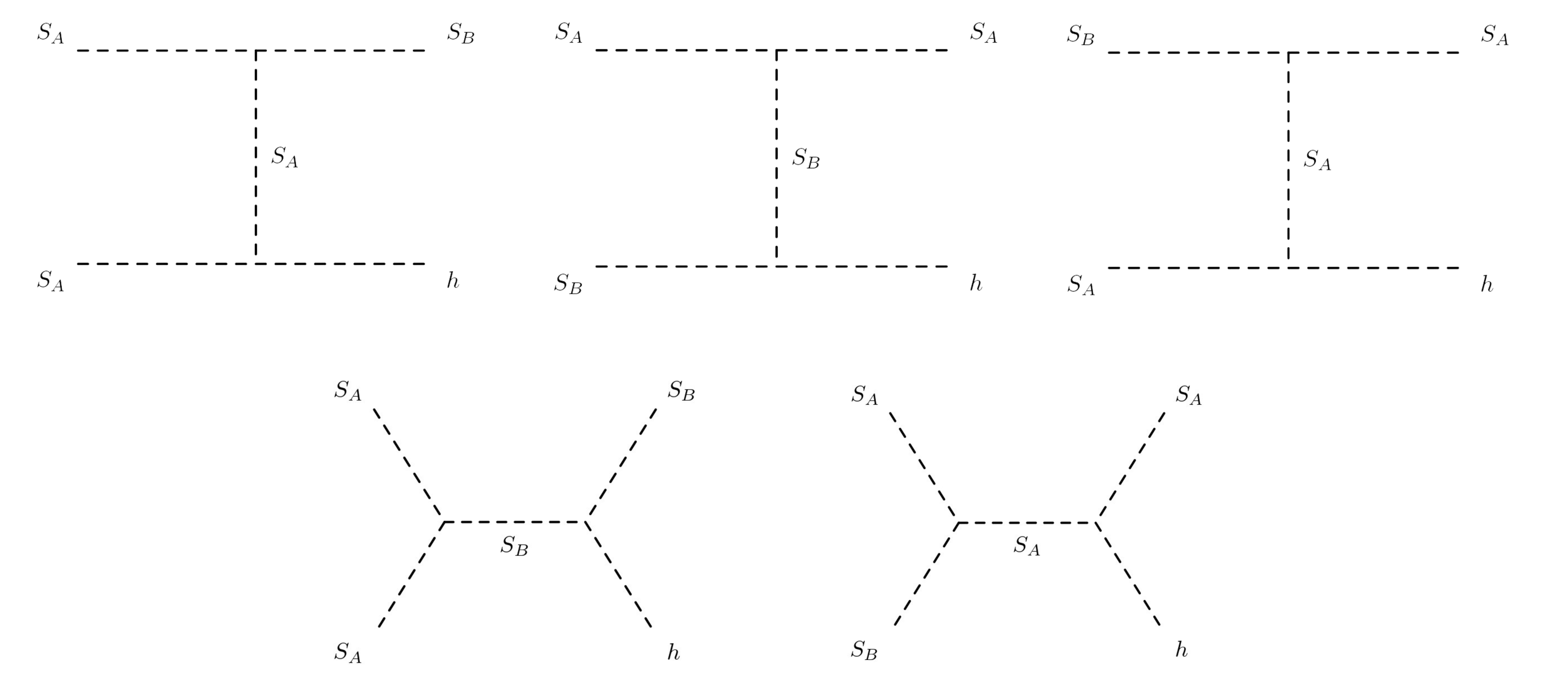
(a) Semi-annihilation processes in the $\mathbb{Z}_{4}$ scenario, driven by the trilinear interaction $\mu_{S1}$ and the Higgs portal coupling $\lambda_{Hi}$.

(b) Semi-annihilation processes in the $\mathbb{Z}_{6}(23)$ scenario (first and second diagram), driven by the trilinear self-interaction term $\mu_{S2}$ and the Higgs portal coupling $\lambda_{Hi}$. Conversion processes in the $\mathbb{Z}_{6}(13)$ scenario (last diagram), driven by the quartic term $\lambda^{\prime}_{AB}$.

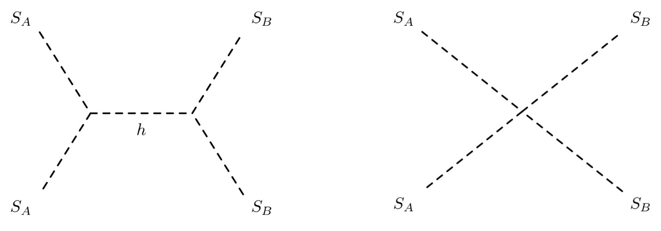
(c) Conversion processes in the $\mathbb{Z}_{4}$ and $\mathbb{Z}_{6}$ scenarios, driven by the quartic interaction term $\lambda_{AB}$ and the Higgs portal coupling $\lambda_{Hi}$.

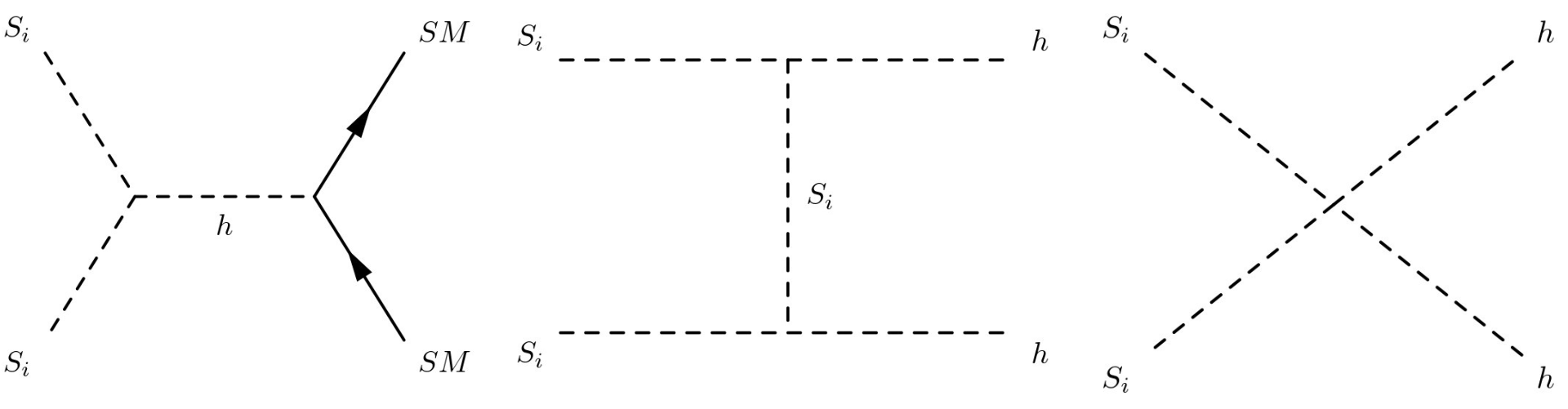
(d) Dark matter $S_{i}$ ($i=A,B$) annihilation processes into SM particles ($\text{SM}=f,h,W\ \text{and}\ Z$), mediated by the Higgs portal couplings $\lambda_{Hi}$. These channels are common to all $\mathbb{Z}_{2n}$ models considered.

Figure 2: Diagrams illustrating the processes in the $\mathbb{Z}_{2n}$ models.

The dark sector dynamics involve three types of interactions: standard annihilation, $S_{i}S_{i}\to\text{SM SM}$ with $i=A,B$ (Fig. 2(d)); conversion, $S_{A}S_{A}^{\dagger}\leftrightarrow S_{B}S_{B}$, mediated by the quartic coupling $\lambda_{AB}$ (Fig. 2(c)); and semi-annihilation, $S_{A}S_{A}\to S_{B}h$, driven by $\mu_{S1}$ and the Higgs portal couplings (Fig. 2(a)). These processes modify the coupled Boltzmann equations as:

$$\begin{split}\dot{n}_{S_{A}}+3Hn_{S_{A}}=&-\langle\sigma v\rangle_{S_{A}S_{A}^{\dagger}\to\text{SM SM}}\left(n_{S_{A}}^{2}-n_{S_{A}}^{\text{eq}\,2}\right)-\langle\sigma v\rangle_{S_{A}S_{A}^{\dagger}\to S_{B}S_{B}}\left(n_{S_{A}}^{2}-n_{S_{B}}^{2}\frac{n_{S_{A}}^{\text{eq}\,2}}{n_{S_{B}}^{\text{eq}\,2}}\right)\\ &-\langle\sigma v\rangle_{S_{A}S_{A}\to S_{B}h}\left(n_{S_{A}}^{2}-n_{S_{A}}^{\text{eq}\,2}\frac{n_{S_{B}}}{n_{S_{B}}^{\text{eq}}}\right),\\ \end{split}$$ (5.2)

$$\begin{split}\dot{n}_{S_{B}}+3Hn_{S_{B}}=&-\langle\sigma v\rangle_{S_{B}S_{B}\to\text{SM SM}}\left(n_{S_{B}}^{2}-n_{S_{B}}^{\text{eq}\,2}\right)-\langle\sigma v\rangle_{S_{B}S_{B}\to S_{A}S_{A}^{\dagger}}\left(n_{S_{B}}^{2}-n_{S_{A}}^{2}\frac{n_{S_{B}}^{\text{eq}\,2}}{n_{S_{A}}^{\text{eq}\,2}}\right)\\ &-\langle\sigma v\rangle_{S_{B}S_{A}\to S_{A}^{\dagger}h}\left(n_{S_{B}}n_{S_{A}}-n_{S_{A}}n_{S_{B}}^{\text{eq}}\right)+\frac{1}{2}\langle\sigma v\rangle_{S_{A}S_{A}\to S_{B}h}\left(n_{S_{A}}^{2}-n_{S_{A}}^{\text{eq}\,2}\frac{n_{S_{B}}}{n_{S_{B}}^{\text{eq}}}\right),\end{split}$$ (5.3)

where the last term in Eq. 5.3 reflects $S_{B}$ re-population from $S_{A}$ semi-annihilation.

5.1.2 $\mathbb{Z}_{6}(23)$ Model

The $\mathbb{Z}_{6}(23)$ model introduces the cubic self-interaction term $\frac{1}{3}\mu_{S2}S_{A}^{3}$ while maintaining $S_{A}$ and $S_{B}$ stability through mass hierarchy constraints. Besides standard annihilation processes, the relic density evolution is primarily governed by two additional mechanisms: dark sector conversion and semi-annihilation. Conversion, mediated by the quartic coupling $\lambda_{AB}$, drives number density exchanges of the form $S_{A}S_{A}^{\dagger}\leftrightarrow S_{B}S_{B}$. Semi-annihilation, enabled by the cubic self-interaction $\mu_{S2}$ in conjunction with the Higgs portal coupling, facilitates processes like $S_{A}S_{A}\to S_{A}^{\dagger}h$. This injects entropy into the visible sector while maintaining approximate thermal equilibrium within the dark sector.

These mechanisms jointly govern freeze-out dynamics, as shown in Figs. 2(b),  2(c) and 2(d). The coupled Boltzmann system becomes:

$$\begin{split}\dot{n}_{S_{A}}+3Hn_{S_{A}}&=-\langle\sigma v\rangle_{S_{A}S_{A}^{\dagger}\to\text{SM SM}}(n_{S_{A}}^{2}-n_{S_{A}}^{\text{eq}\,2})-\langle\sigma v\rangle_{S_{A}S_{A}^{\dagger}\to S_{B}S_{B}}\left(n_{S_{A}}^{2}-n_{S_{B}}^{2}\frac{n_{S_{A}}^{\text{eq}\,2}}{n_{S_{B}}^{\text{eq}\,2}}\right)\\ &\quad-\langle\sigma v\rangle_{S_{A}S_{A}\to S_{A}^{\dagger}h}(n_{S_{A}}^{2}-n_{S_{A}}^{\text{eq}}n_{S_{A}}),\end{split}$$ (5.4)

$$\dot{n}_{S_{B}}+3Hn_{S_{B}}=-\langle\sigma v\rangle_{S_{B}S_{B}\to\text{SM SM}}(n_{S_{B}}^{2}-n_{S_{B}}^{\text{eq}\,2})-\langle\sigma v\rangle_{S_{B}S_{B}\to S_{A}S_{A}^{\dagger}}\left(n_{S_{B}}^{2}-n_{S_{A}}^{2}\frac{n_{S_{B}}^{\text{eq}\,2}}{n_{S_{A}}^{\text{eq}\,2}}\right).$$ (5.5)

5.1.3 $\mathbb{Z}_{6}(13)$ Model

The $\mathbb{Z}_{6}(13)$-symmetric Lagrangian contains the quartic interaction term $\frac{1}{3}\lambda^{\prime}_{AB}S_{A}^{3}S_{B}$, which introduces novel conversion processes between $S_{A}$ and $S_{B}$ while requiring the mass hierarchy $M_{S_{B}}<3M_{S_{A}}$ to prevent $S_{B}\to 3S_{A}$ decays. This ensures both fields remain viable DM components through chemical equilibrium maintenance.

The processes relevant are conversion processes, arising from the quartic interaction terms $\lambda_{AB}$ and $\lambda^{\prime}_{AB}$ and, the standard annihilation. These interactions govern the number densities of $S_{A}$ and $S_{B}$ (Figs. 2(b),  2(c) and  2(d)). These interactions modify the coupled Boltzmann system as:

$$\begin{split}\dot{n}_{S_{A}}+3Hn_{S_{A}}&=-\langle\sigma v\rangle_{S_{A}S_{A}\to\text{SM SM}}\left(n_{S_{A}}^{2}-n_{S_{A}}^{\text{eq}\,2}\right)-\langle\sigma v\rangle_{S_{A}S_{A}^{\dagger}\to S_{B}S_{B}}\left(n_{S_{A}}^{2}-n_{S_{B}}^{2}\frac{n_{S_{A}}^{\text{eq}\,2}}{n_{S_{B}}^{\text{eq}\,2}}\right)\\ &\quad-\langle\sigma v\rangle_{S_{A}S_{A}\to S_{B}S_{A}^{\dagger}}\left(n_{S_{A}}^{2}-n_{S_{A}}^{\text{eq}}n_{S_{A}}\frac{n_{S_{B}}}{n_{S_{B}}^{\text{eq}}}\right),\end{split}$$ (5.6)

$$\begin{split}\dot{n}_{S_{B}}+3Hn_{S_{B}}&=-\langle\sigma v\rangle_{S_{B}S_{B}\to\text{SM SM}}\left(n_{S_{B}}^{2}-n_{S_{B}}^{\text{eq}\,2}\right)-\langle\sigma v\rangle_{S_{B}S_{B}\to S_{A}S_{A}^{\dagger}}\left(n_{S_{B}}^{2}-n_{S_{A}}^{2}\frac{n_{S_{B}}^{\text{eq}\,2}}{n_{S_{A}}^{\text{eq}\,2}}\right)\\ &\quad-\frac{1}{2}\langle\sigma v\rangle_{S_{B}S_{A}\to S_{A}^{\dagger}S_{A}^{\dagger}}\left(n_{S_{B}}n_{S_{A}}-n_{S_{A}}^{2}\frac{n_{S_{B}}^{\text{eq}}}{n_{S_{A}}^{\text{eq}}}\right).\end{split}$$ (5.7)

5.2 Direct Detection

Weakly Interacting Massive Particles (WIMPs), though interacting feebly with ordinary matter, can scatter elastically off atomic nuclei, enabling direct detection via nuclear recoil signatures. Experiments such as XENON1T, LZ, and PandaX-4T search for these rare interactions by measuring keV-scale energy deposits from WIMP-nucleus collisions [84, 85, 86]. At the low momentum transfers relevant for these experiments ($|\vec{q}|\sim 10-100$ MeV), the interaction is coherent over the entire nucleus, making the cross-section primarily sensitive to the nucleus’s mass number $A$.

In $\mathbb{Z}_{2n}$ models, the scalar nature of the DM candidates $S_{A}$ and $S_{B}$ restricts interactions to spin-independent (SI) processes mediated by Higgs exchange. These interactions originate from the Higgs-portal terms in the Lagrangian:

$$\mathcal{L}_{\text{int}}\supset-\lambda_{HA}|H|^{2}|S_{A}|^{2}-\frac{1}{2}\lambda_{HB}|H|^{2}S_{B}^{2},$$ (5.8)

which also govern DM annihilation into SM particles (see Fig. 2(d)). The SI cross-section for a DM particle $S_{i}$ ($i=A,B$) scattering off a nucleus is determined by the coherent enhancement of the interaction across all nucleons. This yields:

$$\sigma_{S_{i}}^{\text{SI}}=\frac{\lambda_{Hi}^{2}f_{N}^{2}}{4\pi}\frac{\mu_{iN}^{2}m_{N}^{2}}{M_{h}^{4}M_{S_{i}}^{2}},$$ (5.9)

where $\lambda_{Hi}$ is the relevant Higgs-portal coupling ($\lambda_{HA}$ for $S_{A}$, $\lambda_{HB}$ for $S_{B}$), $\mu_{iN}=M_{S_{i}}m_{N}/(M_{S_{i}}+m_{N})$ is the WIMP-nucleus reduced mass, $m_{N}$ is the nuclear mass, and $M_{h}\approx 125$ GeV is the Higgs boson mass. The DM particle mass $M_{S_{i}}$ is given by $M_{S_{i}}^{2}=\frac{1}{2}\lambda_{Hi}v^{2}-\mu_{i}^{2}$, where $v\approx 246$ GeV is the Higgs vacuum expectation value. The effective nucleon coupling $f_{N}\approx 0.3$ encapsulates the scalar quark content of the nucleon; however, lattice QCD calculations suggest uncertainties of $\sim 10\%$ in this parameter.

Experimental limits are typically reported as WIMP-nucleon cross-sections, necessitating a conversion from the WIMP-nucleus cross-section. The two are related by:

$$\sigma_{S_{i}}^{\text{SI, nucleon}}=\sigma_{S_{i}}^{\text{SI}}\frac{\mu_{ip}^{2}}{\mu_{iN}^{2}}\frac{1}{A^{2}}\approx\frac{\lambda_{Hi}^{2}f_{p}^{2}}{4\pi}\frac{\mu_{ip}^{2}m_{p}^{2}}{M_{h}^{4}M_{S_{i}}^{2}},$$ (5.10)

where $\mu_{ip}=M_{S_{i}}m_{p}/(M_{S_{i}}+m_{p})$ is the WIMP-proton reduced mass, $m_{p}$ is the proton mass, and $A$ is the nuclear mass number. The approximation $f_{n}\approx f_{p}$ (assuming equivalent neutron and proton scalar couplings) simplifies the analysis, although some theoretical uncertainties remain.

6 Numerical Constraints on $\mathbb{Z}_{2n}$ Dark Matter: Stability, Unitarity, Coupling Perturbativity, and Experiment

We perform a random scan over a subset of the free parameters of the models, simultaneously imposing constraints from vacuum stability, perturbative unitarity, perturbativity of the couplings, the observed DM relic abundance [4], and the non-observation of DM signals in direct detection experiments [84, 85, 86]. For each model, we performed a random scan of approximately $10^{7}$ points, logarithmically distributed over the parameter space, to identify regions consistent with the aforementioned constraints. This scan does not provide a statistical likelihood measure, thus precluding the identification of statistically preferred regions. Our objective is to determine the most influential parameters for model viability and to identify parameter combinations that satisfy all constraints.

Specifically, the total relic density, $\Omega_{S_{A}}h^{2}+\Omega_{S_{B}}h^{2}$, must match the Planck-measured DM abundance: $\Omega_{\text{DM}}h^{2}=0.1200\pm 0.0012$ [4]. We consider a model consistent with this if the calculated relic density falls within $0.108\leq\Omega_{\text{DM}}h^{2}\leq 0.132$, incorporating a conservative 10% theoretical uncertainty. The individual relic densities, $\Omega_{S_{A}}h^{2}$ and $\Omega_{S_{B}}h^{2}$, and their fractional contributions, $\xi_{S_{i}}=\Omega_{S_{i}}h^{2}/\Omega_{\text{DM}}h^{2}$ (where $i=A,B$ and $\xi_{S_{A}}+\xi_{S_{B}}=1$), are computed using micrOMEGAs [87].

We further impose constraints from direct detection. The SI WIMP-nucleon scattering cross-section, $\sigma_{S_{i}}^{\text{SI, nucleon}}$ (see Eq. 5.10), must be below the upper limits from XENON1T, LZ, and PandaX-4T [84, 85, 86]. These experiments strongly constrain Higgs-portal DM models, with micrOMEGAs providing the relevant cross-section calculations.

Following [88], in multi-component DM scenarios, experimental limits on $\sigma_{S_{i}}^{\text{SI, nucleon}}$ are not directly applicable to individual particles. The limits rescale with the fractional contribution of each species to the local DM density. Recoil rates depend on each candidate’s local density; thus, we multiply each $\sigma_{S_{i}}^{\text{SI, nucleon}}$ by its fractional abundance, $\xi_{S_{i}}$. We apply direct detection constraints via:

$$\frac{\xi_{S_{A}}\sigma_{S_{A}}^{\text{SI, nucleon}}}{\sigma_{\text{limit}}(m_{S_{A}})}+\frac{\xi_{S_{B}}\sigma_{S_{B}}^{\text{SI, nucleon}}}{\sigma_{\text{limit}}(m_{S_{B}})}<1,$$ (6.1)

where $\sigma_{\text{limit}}(m_{S_{i}})$ represents the most stringent experimental upper limit on the WIMP-nucleon cross-section for a DM particle of mass $m_{S_{i}}$, considering the results from XENON1T, LZ, and PandaX-4T [84, 85, 86]. The individual cross-sections, $\sigma_{S_{i}}^{\text{SI, nucleon}}$, are computed using micrOMEGAs [87], with Eq. 5.10 serving as a reference for the underlying theoretical framework. For notational simplicity, we will henceforth refer to $\sigma_{S_{i}}^{\text{SI, nucleon}}$ as $\sigma_{S_{i}}^{\text{SI}}$.

Our scans focus on parameter ranges consistent with mass hierarchies allowed by each $\mathbb{Z}_{2n}$ model. While other parameters will be discussed and fixed later, the DM particle masses, $M_{S_{A}}$ and $M_{S_{B}}$, are universally constrained to:

$$40\ \text{GeV}\leq M_{S_{A}},M_{S_{B}}\leq 2\ \text{TeV}.$$ (6.2)

For comparison, we adopt parameter ranges similar to those in [56] where applicable.

Figure 3 summarizes the parameter dependencies for the $\mathbb{Z}_{2n}$ models. Our analysis proceeds by fixing a subset of parameters in each model (see the relevant subsections for details) and performing random scans over the remaining parameters within specified ranges to identify regions consistent with all theoretical and experimental constraints.

Figure 3: Parameter dependencies in the $\mathbb{Z}_{2n}$ models. Filled circles indicate which parameters influence the dark matter observables (relic density and direct detection) and the theoretical constraints (vacuum stability, perturbative unitarity, and coupling perturbativity). Checkmarks ($\checkmark$) denote the presence of each parameter in the specific models ($\mathbb{Z}_{4}$, $\mathbb{Z}_{6}(23)$, and $\mathbb{Z}_{6}(13)$). The parameters $\mu_{S1}$, $\lambda_{S4}$ are specific to the $\mathbb{Z}_{4}$ model, $\mu_{S2}$ is specific to the $\mathbb{Z}_{6}(23)$ and $\lambda^{\prime}_{AB}$ is specific to the $\mathbb{Z}_{6}(13)$ model.

6.1 $\mathbb{Z}_{4}$ Model

As detailed in Fig. 3, the $\mathbb{Z}_{4}$ model’s relic density depends on $\lambda_{HA}$, $\lambda_{HB}$, $\lambda_{AB}$, and $\mu_{S1}$, with direct detection further constraining $\lambda_{HA}$ and $\lambda_{HB}$. All quartic couplings ($\lambda_{A}$, $\lambda_{B}$, $\lambda_{HA}$, $\lambda_{HB}$, $\lambda_{AB}$, and $\lambda_{S4}$) are subject to constraints from vacuum stability, perturbative unitarity, and perturbativity. Because $\mu_{S1}$ only affects the relic density, we treat it as a free parameter, varying it within the range:

$$100\ \text{GeV}\leq\mu_{S1}\leq 10\ \text{TeV}.$$ (6.3)

and exploring its significant impact.

For vacuum stability, perturbative unitarity, and perturbativity, the quartic couplings are crucial. Therefore, we fix these couplings, along with $\lambda_{AB}$, to the specific values presented in Table 2. These values were selected based on the following criteria:

• Vacuum Stability: We require the scalar potential to be bounded from below, ensuring the stability of the electroweak vacuum up to the GUT scale ($\Lambda_{\text{GUT}}\approx 2\times 10^{16}$ GeV) and the Planck scale ($\Lambda_{\text{Pl}}\approx 1.22\times 10^{19}$ GeV). This leads to conditions on the quartic couplings, as detailed in Section 3.

• Perturbative Unitarity: We impose perturbative unitarity constraints on all $2\to 2$ scattering processes involving the scalar fields up to the same energy scales ($\Lambda_{\text{GUT}}$ and $\Lambda_{\text{Pl}}$). This translates into upper bounds on the magnitudes of various combinations of quartic couplings, as discussed in Section 4.

• Perturbativity: We require that the couplings remain perturbative up to the scales $\Lambda_{\text{GUT}}$ and $\Lambda_{\text{Pl}}$. This is enforced by requiring all dimensionless couplings to satisfy $|\lambda_{i}|<4\pi$ (or other suitable bound) at all scales, as determined by the renormalization group equations (RGEs). See Appendix A for details.

Table 2: Fixed coupling values for the two scenarios considered across the $\mathbb{Z}_{2n}$ models. These values satisfy the constraints of vacuum stability, perturbative unitarity, and perturbativity up to the GUT and Planck scales, as determined by a renormalization group equation analysis (see Appendix A). Model-specific parameters are indicated by checkmarks ($\checkmark$) in the “Model Applicability” columns.

			Model Applicability
Coupling	Scenario 1	Scenario 2	$\mathbb{Z}_{4}$	$\mathbb{Z}_{6}(23)$	$\mathbb{Z}_{6}(13)$
$\lambda_{A}$	0.03	0.07	✓	✓	✓
$\lambda_{B}$	0.02	0.035	✓	✓	✓
$\lambda_{AB}$	0.25	-0.05	✓	✓	✓
$\lambda_{S4}$	0.01	0.05	✓	—	—
$\lambda^{\prime}_{AB}$	0.01	0.05	—	—	✓

Similarly, the coupling $\lambda_{AB}$, while also influencing the relic density (see Figure 3), will be fixed to a value that promotes a theoretically consistent scenario. By fixing these quartic couplings, we effectively reduce the dimensionality of the parameter space, allowing for a more focused analysis of the remaining parameters’ impact on DM phenomenology. This approach ensures that our numerical scan explores only regions of parameter space that are theoretically sound.

Within each of the fixed scenarios defined by specific values of $\lambda_{A}$, $\lambda_{B}$, $\lambda_{AB}$, and $\lambda_{S4}$ (see Table 2), we systematically vary the Higgs portal couplings, $\lambda_{HA}$ and $\lambda_{HB}$, along with the DM particle masses $M_{S_{A}}$, $M_{S_{B}}$, and the parameter $\mu_{S1}$. This variation allows us to identify regions of parameter space that simultaneously satisfy all theoretical constraints (vacuum stability up to the GUT/Planck scales, perturbative unitarity up to the GUT/Planck scales, and perturbativity) and experimental bounds (the observed DM relic abundance and non-observation of signals in direct detection experiments).

Our analysis focuses on identifying parameter space points that fulfill the following combined criteria: (i) they yield the correct DM relic abundance, as measured by Planck; (ii) they respect the direct detection limits from XENON1T, LZ, and PandaX-4T; and (iii) they ensure the theoretical consistency of the model, as defined by the aforementioned stability, unitarity, and perturbativity requirements. This approach effectively filters the parameter space, isolating regions compatible with both theoretical principles and experimental observations.

The resulting parameter space scans reveal distinct regions with differing stability properties, see Fig. 4. Red regions indicate parameter combinations that lead to vacuum instability at some energy scale below the Planck scale. A classical stability boundary, represented by a dashed line, separates these unstable regions from regions where the electroweak vacuum is stable at least up to the TeV scale. Within this classically stable region, we further distinguish between areas based on the energy scale up to which stability is maintained. Light green regions denote parameter combinations where vacuum stability holds only up to the GUT scale, while dark green regions indicate stability extending to the Planck scale.

Orange regions, conversely, signify parameter combinations where the electroweak vacuum is classically stable, but where at least one quartic coupling, $|\lambda_{i}|$, exceeds the perturbativity bound of $4\pi$ at some energy scale below the maximum considered (GUT or Planck, depending on the scenario). This signals a breakdown of the perturbative description and suggests the onset of non-perturbative dynamics. Additionally, dot-dashed lines delineate the regions where perturbative unitarity is violated in $2\to 2$ scattering processes involving the scalar fields, considering both the GUT scale (outer dot-dashed line) and the Planck scale (inner dot-dashed line). Notably, the regions excluded by these perturbative unitarity bounds largely overlap with those excluded by the vacuum stability analysis (both classical and quantum-corrected), providing further support for the robustness of our theoretical constraints. The interplay between these theoretically constrained regions and those allowed by DM observables provides a comprehensive picture of the viable parameter space for the $\mathbb{Z}_{4}$ model.

(a) Scenario 1.

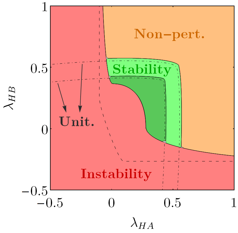
(b) Scenario 2.

Figure 4: Vacuum stability and perturbative unitarity analysis for the $\mathbb{Z}_{4}$ model, showing regions of stability, instability, and non-perturbative behavior in the $(\lambda_{HA},\lambda_{HB})$ plane for two scenarios (see Table 2). Color coding and line styles: dark green (stable up to the Planck scale), light green (stable up to the GUT scale), red (unstable below the Planck scale), orange (classically stable, but with at least one quartic coupling exceeding the perturbativity bound of $|\lambda_{i}|\geq 4\pi$ at some scale below the maximum considered), dot-dashed lines (boundaries where perturbative unitarity is violated: inner line = Planck scale, outer line = GUT scale), dashed lines (classical stability boundaries).

We now present the results of our numerical scans for the $\mathbb{Z}_{4}$ model. As previously established, we fix the quartic couplings $\lambda_{A}$, $\lambda_{B}$, $\lambda_{S4}$, and $\lambda_{AB}$ to the values defined in Table 2 for each of the two scenarios. We then perform independent random scans for each scenario, varying the Higgs portal couplings $\lambda_{HA}$ and $\lambda_{HB}$, the DM particle masses $M_{S_{A}}$ and $M_{S_{B}}$, and the parameter $\mu_{S1}$. We impose the constraint $M_{S_{A}}<M_{S_{B}}$, reflecting the fact that $S_{A}$ is the lighter DM candidate and thus stable against decay to $S_{B}$. The Higgs portal couplings are varied within the range:

$$-1\leq\lambda_{HA},\lambda_{HB}\leq 1.$$ (6.4)

The DM particle masses are constrained to the range given in Eq. 6.2. The parameter $\mu_{S1}$ is varied within the interval defined in Eq. 6.3.

Within this defined parameter space, we select points that simultaneously satisfy the following criteria: (i) they reproduce the observed DM relic abundance (within the 10% theoretical uncertainty, as discussed above); (ii) they are not excluded by the combined direct detection limits from XENON1T, LZ, and PandaX-4T; and (iii) they correspond to a theoretically consistent scenario (vacuum stability and perturbative unitarity up to the GUT or Planck scale, depending on the scenario, and perturbativity, as verified by the RGE analysis in Appendix A). This selection process effectively filters the parameter space, retaining only those regions compatible with both theoretical constraints and experimental observations. We then classify the surviving points based on their stability properties: unstable (dark red), stable up to the GUT scale (light green), and stable up to the Planck scale (dark green). This classification, as visualized in the following figures, reveals the impact of stability considerations on the allowed parameter space.

Our results demonstrate that the combined theoretical constraints of vacuum stability, perturbative unitarity, and perturbativity, along with the experimental bounds from relic density and direct detection, significantly reduce the allowed parameter space. This reduction is particularly noticeable for DM particle masses above 1.5 TeV, but is evident across the entire mass range considered. These findings underscore the importance of incorporating all these constraints in DM model building, complementing and extending previous studies such as [56]. Furthermore, we observe a distinct mass spectrum compared to the single real or complex scalar singlet DM models [38, 89, 39]. While those models exhibit minimum mass thresholds of approximately 959 GeV (real singlet) and 2 TeV (complex singlet) due to XENON1T constraints, the $\mathbb{Z}_{4}$ model allows for viable DM candidates with lower masses.

Having established the impact of theoretical and experimental constraints on the overall parameter space, we now turn to a more detailed examination of the dark matter phenomenology within the allowed regions. Figure 5(a) shows the fractional contribution of $S_{A}$ to the total relic density, $\Omega_{S_{A}}h^{2}/\Omega_{\text{DM}}h^{2}$, as a function of its mass, $M_{S_{A}}$, for both Scenario 1 (left panel) and Scenario 2 (right panel). As expected from the imposed mass hierarchy ($M_{S_{A}}<M_{S_{B}}$), $S_{A}$ is the dominant contributor to the relic density in most of the parameter space. In some cases, the contribution from $S_{B}$ is suppressed by several orders of magnitude.

Figure 5(b) displays the relationship between $M_{S_{A}}$ and $\mu_{S1}$ for both scenarios. We observe that the allowed values of $\mu_{S1}$ span nearly the entire range considered, with a noticeable concentration of points near the upper limit of $\mu_{S1}\sim 10$ TeV for $M_{S_{A}}$ values approaching 1 TeV. This concentration may be due to the increased importance of semi-annihilation processes at higher values of $\mu_{S1}$, which can efficiently deplete the relic density and allow for larger values of $M_{S_{A}}$ to be consistent with the observed abundance.

Figure 5(c) presents the relationship between the DM particle masses, specifically $M_{S_{A}}$ versus the mass ratio $M_{S_{B}}/M_{S_{A}}$, for both scenarios. Notably, the allowed points exhibit no degeneracy between $M_{S_{A}}$ and $M_{S_{B}}$ (i.e., $M_{S_{B}}/M_{S_{A}}>1$), which is a desirable feature for DM model building, as it allows for a clear distinction between the two DM candidates, for example, in collider searches or indirect detection signals.

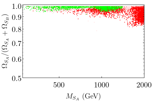
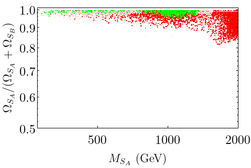
(a) Fractional contribution of $S_{A}$ to the total relic density ($\Omega_{S_{A}}h^{2}/\Omega_{\text{DM}}h^{2}$) as a function of $M_{S_{A}}$ for Scenario 1 (left) and Scenario 2 (right). The color coding indicates the stability region: dark red (unstable), light red (stable up to the GUT scale), and green (stable up to the Planck scale).

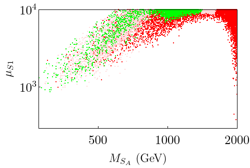
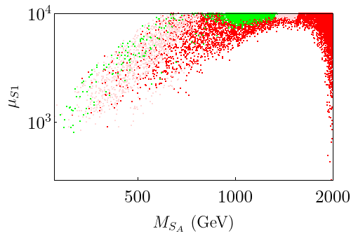
(b) Relationship between $M_{S_{A}}$ and $\mu_{S1}$ for Scenario 1 (left) and Scenario 2 (right). The color coding is the same as in Fig. 5(a).

(c) Mass ratio $M_{S_{B}}/M_{S_{A}}$ as a function of $M_{S_{A}}$ for Scenario 1 (left) and Scenario 2 (right). The color coding is the same as in Fig. 5(a).

Figure 5: Numerical results for the $\mathbb{Z}_{4}$ model, showing the interplay between dark matter observables, the parameter $\mu_{S1}$, and the stability constraints. See subcaptions for details.

We now turn to the direct detection prospects of the $\mathbb{Z}_{4}$ model. Figure 6 shows the rescaled spin-independent WIMP-nucleon scattering cross-section, $\xi_{S_{i}}\sigma_{S_{i}}^{\text{SI}}$, as a function of the DM particle mass, $M_{S_{i}}$, for both $S_{A}$ (top panels) and $S_{B}$ (bottom panels), and for both Scenario 1 (left panels) and Scenario 2 (right panels). As expected from our selection criteria, all points satisfy the current XENON1T bound [84]. While incorporating the more stringent limits from PandaX-4T [86] and LUX-ZEPLIN (LZ) [85] would further constrain the parameter space, a significant number of points remain viable. We also display the neutrino floor [90], representing the ultimate sensitivity limit for direct detection experiments due to coherent neutrino scattering. A considerable fraction of the allowed parameter space lies above the neutrino floor, indicating potential for future discovery.

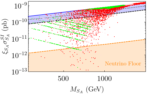
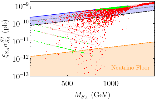
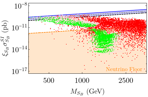
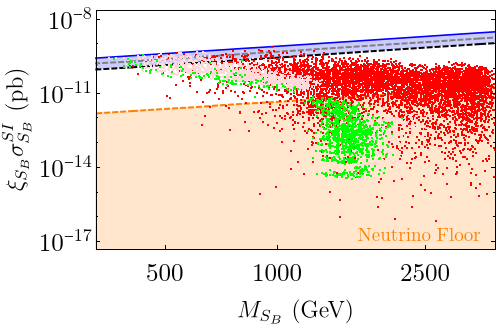
Figure 6: Direct detection prospects for the $\mathbb{Z}_{4}$ model. Top panels: $\xi_{S_{A}}\sigma_{S_{A}}^{\text{SI}}$ vs. $M_{S_{A}}$. Bottom panels: $\xi_{S_{B}}\sigma_{S_{B}}^{\text{SI}}$ vs. $M_{S_{B}}$. Left panels: Scenario 1. Right panels: Scenario 2. Color coding represents stability regions: dark red (unstable), light red (stable up to the GUT scale), green (stable up to the Planck scale). Experimental limits: solid blue (XENON1T [84]), dashed gray (PandaX-4T [86]), dashed black (LUX-ZEPLIN (LZ) [85]). The dashed orange line indicates the neutrino floor [90].

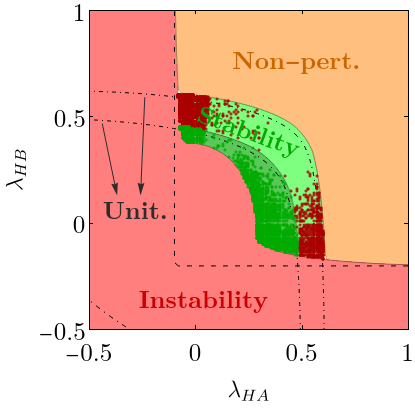
(a) Scenario 1.

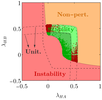
(b) Scenario 2.

Figure 7: Allowed regions in the $(\lambda_{HA},\lambda_{HB})$ plane for the $\mathbb{Z}_{4}$ model, illustrating the combined constraints from vacuum stability, perturbative unitarity, coupling perturbativity, and dark matter. Scenario 1 is shown in the left panel, and Scenario 2 in the right panel. Refer to Fig. 4 for the color coding and line style definitions. Red and green points within the theoretically consistent regions additionally satisfy relic density and direct detection constraints.

Figure 7 focuses on the ($\lambda_{HA}$, $\lambda_{HB}$) plane regions satisfying vacuum stability, perturbative unitarity, and coupling perturbativity up to the GUT and Planck scales. For each scenario (Scenario 1: left panel; Scenario 2: right panel), after fixing the remaining quartic couplings as per Table 2, we identify ($\lambda_{HA}$, $\lambda_{HB}$) combinations that also yield the correct relic density and are consistent with direct detection limits. Green and red points represent parameter combinations meeting these dark matter constraints and satisfying stability, unitarity, and perturbativity up to the Planck and GUT scales, respectively. A significant portion of the scanned ($\lambda_{HA}$, $\lambda_{HB}$) parameter space is theoretically viable and consistent with these constraints, especially for Planck-scale stability, though complete coverage is not observed in either scenario.

The qualitative similarity between the results for Scenario 1 and Scenario 2, particularly the shapes of the regions allowed by vacuum stability and perturbative unitarity in the $(\lambda_{HA},\lambda_{HB})$ plane, indicates that the overall features of the viable parameter space are relatively insensitive to the specific choices of the fixed quartic couplings ($\lambda_{A}$, $\lambda_{B}$, $\lambda_{AB}$, and, for the $\mathbb{Z}_{4}$ model, $\lambda_{S4}$) within the ranges considered. Therefore, for subsequent $\mathbb{Z}_{2n}$ models, while we will continue to analyze two distinct scenarios to ensure robustness, we will often focus the graphical representation of results on a single, representative scenario to avoid unnecessary repetition.

6.2 $\mathbb{Z}_{6}(23)$ model

Turning to the $\mathbb{Z}_{6}(23)$ model, Fig. 3 details its parameter dependencies. The relic density is determined by $\lambda_{HA}$, $\lambda_{HB}$, $\lambda_{AB}$, and $\mu_{S2}$, while direct detection again constrains the Higgs portal couplings. As with the $\mathbb{Z}_{4}$ model, vacuum stability, perturbative unitarity, and tree-level perturbativity restrict all quartic couplings ($\lambda_{A}$, $\lambda_{B}$, $\lambda_{HA}$, $\lambda_{HB}$, and $\lambda_{AB}$). Crucially, the $\mathbb{Z}_{6}(23)$ model features $\mu_{S2}$ in place of $\mu_{S1}$ and excludes the $\lambda_{S4}$ term.

As with $\mu_{S1}$ in the $\mathbb{Z}_{4}$ model, $\mu_{S2}$ influences only the relic density and is not directly constrained by stability, unitarity, or direct detection. Therefore, we treat $\mu_{S2}$ as a free parameter, varying it within the range:

$$100\ \text{GeV}\leq\mu_{S2}\leq 10\ \text{TeV}.$$ (6.5)

Although both parameters significantly impact the relic density, they originate from distinct interaction terms: $\mu_{S1}$ (in the $\mathbb{Z}_{4}$ model) couples $S_{A}$ and $S_{B}$, while $\mu_{S2}$ arises from a self-interaction term for $S_{A}$ (see Section 2 for details).

To ensure theoretical consistency, we fix the quartic couplings $\lambda_{A}$, $\lambda_{B}$, and $\lambda_{AB}$ to specific values, presented in Table 2, that satisfy the requirements of vacuum stability, perturbative unitarity, and perturbativity (all considered up to the GUT and Planck scales). We consider two distinct scenarios, analogous to those in the $\mathbb{Z}_{4}$ model, but with $\lambda_{S4}=0$. The resulting stability regions in the $(\lambda_{HA},\lambda_{HB})$ plane, shown in Fig. 8, are qualitatively similar to those of the $\mathbb{Z}_{4}$ model (compare with Fig. 4).

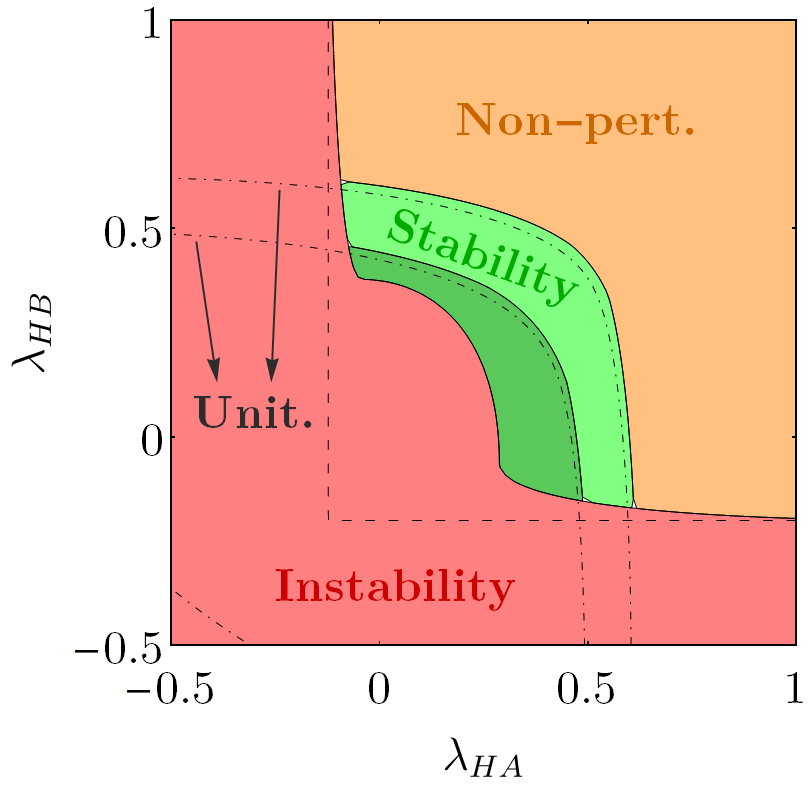
(a) Scenario 1.

(b) Scenario 2.

Figure 8: Vacuum stability and perturbative unitarity analysis for the $\mathbb{Z}_{6}(23)$ model (Scenario 1 and 2 on the left and right panels, respectively), analogous to Fig. 4 but with $\lambda_{S4}=0$. Regions of stability and instability are shown in the $(\lambda_{HA},\lambda_{HB})$ plane. See Fig. 4 for the color coding and line style definitions.

We now vary the DM particle masses, $M_{S_{A}}$ and $M_{S_{B}}$, the parameter $\mu_{S2}$, and the Higgs portal couplings, $\lambda_{HA}$ and $\lambda_{HB}$, performing independent random scans for each scenario defined in Table 2. While the $\mathbb{Z}_{6}(23)$ model itself does not impose a strict mass hierarchy, for these scans we maintain the condition $M_{S_{A}}<M_{S_{B}}$, analogous to the $\mathbb{Z}_{4}$ analysis. The Higgs portal couplings are varied within the range:

$$-1\leq\lambda_{HA},\lambda_{HB}\leq 1.$$ (6.6)

As in the $\mathbb{Z}_{4}$ case, the constraints of vacuum stability, perturbative unitarity, and perturbativity remain crucial. However, in the $\mathbb{Z}_{6}(23)$ model, we find a significantly higher proportion of parameter space points that simultaneously satisfy these theoretical constraints and the constraints from DM observables. Notably, a large fraction of the allowed points exhibit stability up to the Planck scale. Furthermore, similar to the $\mathbb{Z}_{4}$ model, the $\mathbb{Z}_{6}(23)$ model allows for viable DM candidates with masses below the minimum thresholds found in typical real and complex singlet scalar DM models (approximately 959 GeV and 2 TeV, respectively) [38, 89, 39], with a significant concentration of allowed points below 1 TeV.

Figure 9(a) displays the fractional contribution of $S_{A}$ to the total relic density ($\Omega_{S_{A}}h^{2}/\Omega_{\text{DM}}h^{2}$) as a function of $M_{S_{A}}$ for Scenario 1. Unlike the $\mathbb{Z}_{4}$ model, where $S_{A}$ typically dominated, both $S_{A}$ and $S_{B}$ can contribute significantly in the $\mathbb{Z}_{6}(23)$ case.

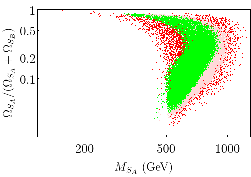
(a) Fractional $S_{A}$ contribution to the total relic density, ($\Omega_{S_{A}}h^{2}/\Omega_{\text{DM}}h^{2}$) as a function of $M_{S_{A}}$ for the $\mathbb{Z}_{6}(23)$ model (Scenario 1). Color coding indicates stability regions: dark red (unstable), light red (stable up to the GUT scale), and green (stable up to the Planck scale).

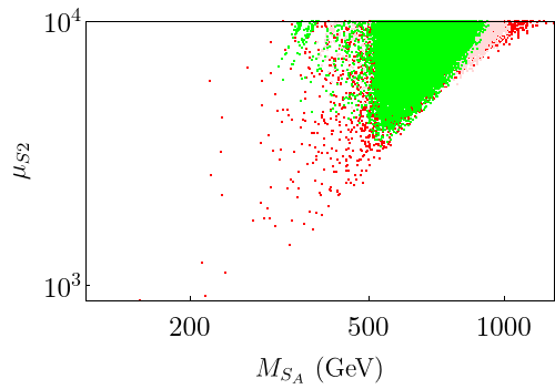
(b) Relationship between $M_{S_{A}}$ and $\mu_{S2}$ for the $\mathbb{Z}_{6}(23)$ model (Scenario 1). Color coding is the same as in Fig. 9(a).

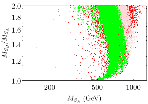
(c) Mass ratio $M_{S_{B}}/M_{S_{A}}$ as a function of $M_{S_{A}}$ for the $\mathbb{Z}_{6}(23)$ model (Scenario 1). Color coding is the same as in Fig. 9(a).

Figure 9: Numerical results for the $\mathbb{Z}_{6}(23)$ model, showing the interplay between dark matter observables, the parameter $\mu_{S2}$, and the stability constraints. See subcaptions for details.

Figure 9(b) shows the relationship between $M_{S_{A}}$ and the parameter $\mu_{S2}$ for Scenario 1. Allowed values of $\mu_{S2}$ span a considerable portion of the considered range ($100\text{ GeV}\leq\mu_{S2}\leq 10\text{ TeV}$), with a noticeable concentration of points near the upper limit as $M_{S_{A}}$ approaches 1 TeV. This concentration may reflect the increased importance of semi-annihilation processes, governed by $\mu_{S2}$, in achieving the correct relic density at higher DM masses.

Figure 9(c) depicts the mass ratio $M_{S_{B}}/M_{S_{A}}$ as a function of $M_{S_{A}}$ for Scenario 1. As imposed in our scan, $M_{S_{B}}>M_{S_{A}}$, ensuring no degeneracy between the two DM candidates. This mass hierarchy facilitates the potential for distinct experimental signatures for each particle.

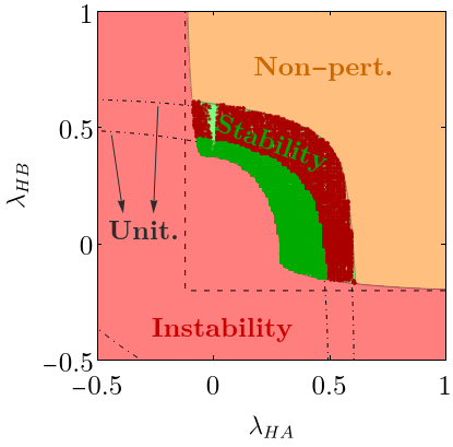
Figure 10: Allowed regions in the $(\lambda_{HA},\lambda_{HB})$ plane for Scenario 1 of the $\mathbb{Z}_{6}(23)$ model. These regions represent parameter combinations that simultaneously satisfy theoretical constraints (up to the GUT and Planck scales) and dark matter constraints. Red and green points within the stability regions satisfy all constraints. Compare with Fig. 7 for the corresponding results in the $\mathbb{Z}_{4}$ model.

Figure 10 focuses on the $(\lambda_{HA},\lambda_{HB})$ plane for Scenario 1 of the $\mathbb{Z}_{6}(23)$ model. It displays regions, indicated by green and red points, that simultaneously satisfy theoretical constraints up to the GUT and Planck scales, as well as dark matter constraints. A significant portion of the scanned $(\lambda_{HA},\lambda_{HB})$ parameter space is found to be both theoretically viable and consistent with dark matter constraints. This is particularly true for parameter combinations that satisfy the Planck-scale requirements.

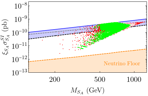
(a) $\xi_{S_{A}}\sigma_{S_{A}}^{\text{SI}}$ vs. $M_{S_{A}}$ for the $\mathbb{Z}_{6}(23)$ model (Scenario 1).

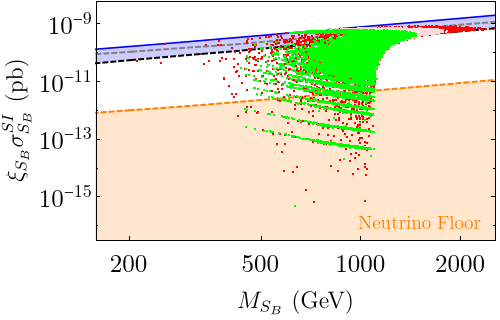
(b) $\xi_{S_{B}}\sigma_{S_{B}}^{\text{SI}}$ vs. $M_{S_{B}}$ for the $\mathbb{Z}_{6}(23)$ model (Scenario 1).

Figure 11: Direct detection prospects for the $\mathbb{Z}_{6}(23)$ model (Scenario 1). (a) Rescaled cross-section for $S_{A}$. (b) Rescaled cross-section for $S_{B}$. Color coding represents stability regions: dark red (unstable), light red (stable up to the GUT scale), green (stable up to the Planck scale). Experimental limits: solid blue (XENON1T [84]), dashed gray (PandaX-4T [86]), dashed black (LUX-ZEPLIN (LZ) [85]). Dashed orange: neutrino floor [90].

Turning to the direct detection prospects for the $\mathbb{Z}_{6}(23)$ model, Fig. 11 displays the rescaled spin-independent WIMP-nucleon scattering cross-sections, $\xi_{S_{A}}\sigma_{S_{A}}^{\text{SI}}$ (left panel) and $\xi_{S_{B}}\sigma_{S_{B}}^{\text{SI}}$ (right panel), as functions of the respective DM particle masses, $M_{S_{A}}$ and $M_{S_{B}}$, for Scenario 1. As anticipated by our selection criteria, all generated points satisfy the current XENON1T bound [84]. Although incorporating the more stringent limits from PandaX-4T [86] and LUX-ZEPLIN (LZ) [85] would further reduce the allowed parameter space, a substantial number of points remain viable. The neutrino floor [90], representing the ultimate sensitivity limit for WIMP direct detection due to coherent neutrino scattering, is also shown. Notably, all points for $S_{A}$, and a significant fraction for $S_{B}$, lie above the neutrino floor, suggesting potential for detection in future experiments.

6.3 $\mathbb{Z}_{6}(13)$ model

The $\mathbb{Z}_{6}(13)$ model’s relic density exhibits distinct dependence on four key couplings: the Higgs-portal terms ($\lambda_{HA}$, $\lambda_{HB}$), the dark sector quartic interaction $\lambda_{AB}$, and the symmetry-driven coupling $\lambda^{\prime}_{AB}$, which enables $S_{A}^{3}S_{B}$ interactions critical for number density conversion (Fig. 3). While direct detection experiments constrain only the Higgs-portal couplings $\lambda_{HA}$ and $\lambda_{HB}$, theoretical consistency – enforced through vacuum stability, perturbative unitarity, and coupling perturbativity – imposes bounds on the full quartic sector: the scalar self-couplings ($\lambda_{A}$, $\lambda_{B}$), portal terms ($\lambda_{HA}$, $\lambda_{HB}$, $\lambda_{AB}$), and the $\mathbb{Z}_{6}(13)$-specific operator $\lambda^{\prime}_{AB}$. This interplay between $\lambda^{\prime}_{AB}$-dependent freeze-out dynamics and multi-scale theoretical constraints creates a tightly regulated parameter space unique to the $\mathbb{Z}_{6}^{(13)}$ framework.

Unlike the previous models, the $\mathbb{Z}_{6}(13)$ model has no free parameter analogous to $\mu_{S1}$ or $\mu_{S2}$. Therefore, to ensure theoretical consistency, all quartic couplings, including $\lambda^{\prime}_{AB}$, are fixed to the values presented in Table 2. The values for $\lambda^{\prime}_{AB}$ mirror those used for $\lambda_{S4}$ in the $\mathbb{Z}_{4}$ model. This leaves only the DM particle masses, $M_{S_{A}}$ and $M_{S_{B}}$ (with the imposed hierarchy $M_{S_{A}}<M_{S_{B}}$), and the Higgs portal couplings, $\lambda_{HA}$ and $\lambda_{HB}$ (varied within $-1\leq\lambda_{HA},\lambda_{HB}\leq 1$), as free parameters in our scans. We consider two scenarios, as defined by the common parameter values in Table 2. Given the similarities in stability regions observed across scenarios in previous models, we present results only for Scenario 1 to avoid redundancy. The methodology is consistent with that employed for the $\mathbb{Z}_{4}$ and $\mathbb{Z}_{6}(23)$ models.

Figure 12 displays the regions in the $(\lambda_{HA},\lambda_{HB})$ plane for Scenario 1 that remain viable after imposing all theoretical constraints, which, as anticipated, are qualitatively similar to those of the other models.

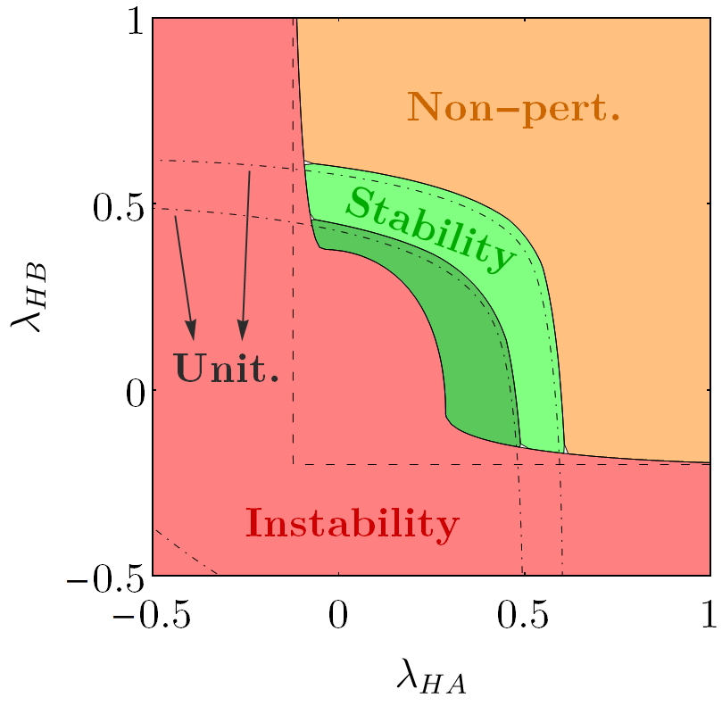
(a) Scenario 1.

(b) Scenario 2.

Figure 12: One-loop vacuum stability and instability regions, evaluated from the top quark mass scale up to the GUT and Planck scales. The dark green region indicates stability up to the Planck scale, with all quartic scalar couplings remaining perturbative. The red region denotes instability extending to the Planck scale. The light green area expands the stable region if stability is only required up to the GUT scale. Orange regions represent scenarios that appear stable but involve non-perturbative dynamics due to a quartic coupling $\lambda_{i}$ exceeding $4\pi$. Dashed curves indicate the classical boundaries between stable and unstable regions. Dot-dashed lines represent the boundaries where perturbative unitarity is violated (inner line: Planck scale, outer line: GUT scale).

In the $\mathbb{Z}_{6}(13)$ model, the constraints of vacuum stability, perturbative unitarity, and perturbativity remain significant, as expected. However, in contrast to the previous models, the allowed parameter space is more restricted. Figures 13(a) through 14(b) show that the majority of the points satisfying all constraints cluster around the Higgs resonance region ($M_{S_{A}}\approx M_{h}/2$) and near the upper mass limit of our scan (2 TeV). This restricted distribution is a direct consequence of fixing $\lambda^{\prime}_{AB}$ to the values given in Table 2, thus eliminating a degree of freedom that, in the other models, allowed for a broader range of viable parameter combinations.

While the $\mathbb{Z}_{6}(13)$ model presents an interesting theoretical framework, previous work [56] has shown that it faces significant challenges in simultaneously satisfying relic density and direct detection constraints, limiting its viability as a complete DM explanation.

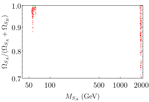
(a) Fractional $S_{A}$ contribution to the total relic density, ($\Omega_{S_{A}}h^{2}/\Omega_{\text{DM}}h^{2}$) as a function of $M_{S_{A}}$ for the $\mathbb{Z}_{6}(13)$ model (Scenario 1). Color coding indicates stability regions: dark red (unstable), light red (stable up to the GUT scale), and green (stable up to the Planck scale).

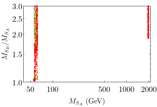
(b) Mass ratio $M_{S_{B}}/M_{S_{A}}$ as a function of $M_{S_{A}}$ for the $\mathbb{Z}_{6}(13)$ model (Scenario 1). Color coding is the same as in Fig. 13(a).

Figure 13: Numerical results for the $\mathbb{Z}_{6}(13)$ model. See subcaptions for details.

Figure 13(a) displays the fractional contribution of $S_{A}$ to the total relic density ($\Omega_{S_{A}}h^{2}/\Omega_{\text{DM}}h^{2}$) as a function of $M_{S_{A}}$ for Scenario 1 of the $\mathbb{Z}_{6}(13)$ model. In this model, where all quartic couplings, including $\lambda^{\prime}_{AB}$, are fixed, we find that $S_{A}$ is the primary contributor to the relic density while simultaneously satisfying all theoretical and experimental constraints.

Figure 13(b) depicts the mass ratio $M_{S_{B}}/M_{S_{A}}$ as a function of $M_{S_{A}}$ for Scenario 1. As imposed in our scan, $M_{S_{B}}>M_{S_{A}}$, ensuring no degeneracy between the two DM candidates. This mass hierarchy facilitates the potential for distinct experimental signatures for each particle.

We now examine the direct detection prospects for the $\mathbb{Z}_{6}(13)$ model. Figure 14 presents the rescaled spin-independent WIMP-nucleon scattering cross-sections, $\xi_{S_{A}}\sigma_{S_{A}}^{\text{SI}}$ (left panel) and $\xi_{S_{B}}\sigma_{S_{B}}^{\text{SI}}$ (right panel), as functions of the respective DM particle masses, $M_{S_{A}}$ and $M_{S_{B}}$, for Scenario 1. All generated points satisfy the current XENON1T bound [84], consistent with our selection criteria. While the more stringent limits from PandaX-4T [86] and LUX-ZEPLIN (LZ) [85] would further constrain the parameter space, a significant number of points remain viable. The neutrino floor [90], representing the ultimate sensitivity limit for WIMP direct detection due to coherent neutrino-nucleus scattering, is also shown. Notably, nearly all generated points for $S_{A}$, and a considerable fraction for $S_{B}$, lie above the neutrino floor, indicating the potential for discovery in future direct detection experiments.

In contrast to the $\mathbb{Z}_{4}$ and $\mathbb{Z}_{6}(23)$ models, the $\mathbb{Z}_{6}(13)$ model yields a significantly smaller viable parameter space due to the fixed value of $\lambda^{\prime}_{AB}$. The number of points satisfying all theoretical and experimental constraints is insufficient to produce a meaningful graphical representation of the allowed regions in the $(\lambda_{HA},\lambda_{HB})$ plane, analogous to Figs. 7 and 10. Therefore, we do not include such a figure.

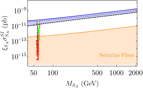
(a) $\xi_{S_{A}}\sigma_{S_{A}}^{\text{SI}}$ vs. $M_{S_{A}}$ for the $\mathbb{Z}_{6}(13)$ model (Scenario 1).

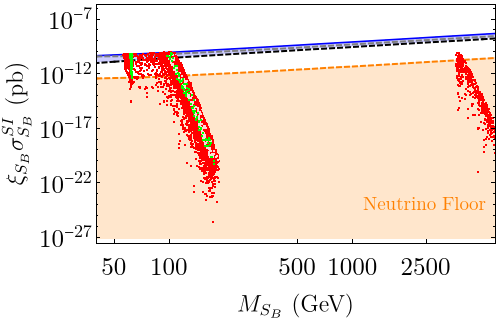
(b) $\xi_{S_{B}}\sigma_{S_{B}}^{\text{SI}}$ vs. $M_{S_{B}}$ for the $\mathbb{Z}_{6}(13)$ model (Scenario 1).

Figure 14: Direct detection prospects for the $\mathbb{Z}_{6}(13)$ model (Scenario 1). Color coding represents stability regions: dark red (unstable), light red (stable up to the GUT scale), green (stable up to the Planck scale). Experimental limits: solid blue (XENON1T [84]), dashed gray (PandaX-4T [86]), dashed black (LUX-ZEPLIN (LZ) [85]). Dashed orange: neutrino floor [90].

7 Conclusions

This work has investigated the viability of two-component scalar dark matter (DM) models stabilized by a $\mathbb{Z}_{2n}$ symmetry, focusing on three specific cases: $\mathbb{Z}_{4}$, $\mathbb{Z}_{6}(23)$, and $\mathbb{Z}_{6}(13)$. These models, originally proposed in Ref. [56], extend the Standard Model (SM) with a complex scalar singlet ($S_{A}$) and a real scalar singlet ($S_{B}$), and feature interactions mediated by Higgs portal couplings and additional quartic couplings. We performed a comprehensive numerical analysis, simultaneously imposing constraints from DM relic abundance (using Planck data [4]), direct detection limits (from XENON1T, LZ, and PandaX-4T [84, 85, 86]), and theoretical requirements of vacuum stability, perturbative unitarity, and coupling perturbativity up to the GUT and Planck scales. The high-energy behavior of the couplings was determined using one-loop Renormalization Group Equations (RGEs), and the method of Ref. [71] was employed to ensure the validity of the vacuum stability analysis at all scales.

Our results demonstrate that these $\mathbb{Z}_{2n}$ models can provide viable two-component DM scenarios consistent with all imposed constraints, for a range of DM masses and couplings. We identified regions of parameter space, primarily within the plane of the Higgs portal couplings ($\lambda_{HA}$, $\lambda_{HB}$) and DM particle masses ($M_{S_{A}}$, $M_{S_{B}}$), that satisfy the observed relic density and remain compatible with current direct detection limits.

The $\mathbb{Z}_{4}$ and $\mathbb{Z}_{6}(23)$ models exhibit several similarities. Both feature semi-annihilation processes, driven by the trilinear couplings $\mu_{S1}$ ($\mathbb{Z}_{4}$) and $\mu_{S2}$ ($\mathbb{Z}_{6}(23)$), respectively, which significantly impact the relic density. In the $\mathbb{Z}_{4}$ model, the imposed mass hierarchy ($M_{S_{B}}<2M_{S_{A}}$) typically resulted in $S_{A}$ being the dominant DM component. The $\mathbb{Z}_{6}(23)$ model, however, allowed for significant contributions to the relic density from both $S_{A}$ and $S_{B}$. In both models, we found viable DM candidates with masses below the typical thresholds seen in single-scalar singlet extensions of the SM, and a noticeable concentration of allowed points was observed near the upper limit of the scanned $\mu_{S1}$/$\mu_{S2}$ range, potentially due to the increased efficiency of semi-annihilation. Direct detection experiments, particularly XENON1T, LZ, and PandaX-4T, placed significant constraints on the Higgs portal couplings, but substantial regions of parameter space remain viable, with many points lying above the neutrino floor.

The $\mathbb{Z}_{6}(13)$ model, on the other hand, presented a distinct scenario. To ensure theoretical consistency, all quartic couplings, including $\lambda^{\prime}_{AB}$, were fixed. This eliminated a key degree of freedom present in the other models, resulting in a more restricted viable parameter space. The surviving points clustered primarily around the Higgs resonance region and near the upper mass limit of our scan, with $S_{A}$ being the dominant DM contributor. Despite these restrictions, viable regions consistent with all constraints, including direct detection limits and the neutrino floor, were identified.

While these models were initially proposed in Ref. [56], our work significantly extends the analysis by incorporating stringent theoretical constraints – vacuum stability, perturbative unitarity, and coupling perturbativity – enforced up to the GUT and Planck scales using RGEs. This combined analysis, integrating both theoretical and experimental constraints, is crucial for a complete assessment of model viability and considerably reduces the allowed parameter space compared to analyses focused solely on dark matter phenomenology.

Future research will focus on two primary directions: (1) a detailed numerical study of phase transitions in the early Universe within these $\mathbb{Z}_{2n}$ models and the potential generation of observable gravitational wave signals; and (2) an investigation of supersymmetric extensions of these models. While collider phenomenology, indirect detection constraints, and the regions near the neutrino floor remain interesting avenues for exploration, the aforementioned topics will be prioritized. This work establishes $\mathbb{Z}_{2n}$-symmetric multicomponent DM as a compelling paradigm, bridging high-scale particle physics with observable phenomena.

Appendix A One-Loop Renormalization Group Equations

We present the one-loop Renormalization Group Equations (RGEs) for all models considered in this work. In the context of vacuum stability, the relevant RGEs govern the evolution of gauge couplings, quartic scalar couplings, and the top Yukawa coupling, as all other Yukawa interactions are neglected.

The renormalization scale $\mu$ ranges from the top quark mass, $M_{t}=172.69\ \mbox{GeV}$ [91], up to the Planck scale, $1.22\times 10^{19}\ \mbox{GeV}$, with $t=\ln\mu$. Below, we first present the RGEs common to all models, followed by the model-specific contributions.

A.1 RGEs: Universal Terms and Model-Dependent Contributions

Gauge and Yukawa Coupling RGEs (Common to All Models)

The RGEs for the gauge couplings and the top Yukawa coupling ($y_{t}$) remain unchanged from the Standard Model (SM):

$$(4\pi)^{2}\frac{dg_{i}}{dt} =b_{i}g_{i}^{3},\quad\text{with}\quad b_{i}=\left(\frac{41}{10},-\frac{19}{6},-7\right),$$ (A.1)

$$(4\pi)^{2}\frac{dy_{t}}{dt} =y_{t}\left(-\frac{17}{20}g_{1}^{2}-\frac{9}{4}g_{2}^{2}-8g_{3}^{2}+\frac{9}{2}y_{t}^{2}\right).$$ (A.2)

Here, $g_{1}$, $g_{2}$, and $g_{3}$ are the gauge couplings of $\mathrm{U}(1)_{Y}$, $\mathrm{SU}(2)_{L}$, and $\mathrm{SU}(3)_{C}$, respectively. We adopt the Grand Unified Theory GUT-inspired normalization, where $g_{1}\equiv\sqrt{5/3}\,g_{Y}$.

Quartic Coupling RGEs (Common to All Models)

The RGEs for the quartic scalar couplings incorporate corrections from gauge, Yukawa, and scalar interactions:

$$\begin{split}(4\pi)^{2}\frac{d\lambda_{H}}{dt}&=\frac{27}{200}g_{1}^{4}+\frac{9}{20}g_{1}^{2}g_{2}^{2}+\frac{9}{8}g_{2}^{4}-9\lambda_{H}\left(\frac{1}{5}g_{1}^{2}+g_{2}^{2}\right)\\ &\quad+24\lambda_{H}^{2}+12\lambda_{H}y_{t}^{2}-6y_{t}^{4}+\lambda_{HA}^{2}+\frac{1}{2}\lambda_{HB}^{2},\end{split}$$ (A.3)

$$(4\pi)^{2}\frac{d\lambda_{B}}{dt} =72\lambda_{B}^{2}+\lambda_{AB}^{2}+\frac{1}{2}\lambda_{HB}^{2},$$ (A.4)

$$(4\pi)^{2}\frac{d\lambda_{HA}}{dt} =-\frac{9}{2}\lambda_{HA}\left(\frac{1}{5}g_{1}^{2}+g_{2}^{2}\right)+2\lambda_{HA}\left(6\lambda_{H}+4\lambda_{A}+2\lambda_{HA}+3y_{t}^{2}\right)+2\lambda_{AB}\lambda_{HB},$$ (A.5)

$$(4\pi)^{2}\frac{d\lambda_{HB}}{dt} =-\frac{9}{2}\lambda_{HB}\left(\frac{1}{5}g_{1}^{2}+g_{2}^{2}\right)+6\lambda_{HB}\left(2\lambda_{H}+4\lambda_{B}+y_{t}^{2}\right)+4\lambda_{AB}\lambda_{HA}+4\lambda_{HB}^{2}.$$ (A.6)

The RGE for the Higgs self-coupling ($\lambda_{H}$) differs from the SM due to the additional terms $\lambda_{HA}^{2}$ and $\frac{1}{2}\lambda_{HB}^{2}$.

Model-Specific Quartic Coupling RGEs

The additional RGEs for the quartic scalar couplings in each model are as follows.

For the $\mathbb{Z}_{4}$ model:

$$(4\pi)^{2}\frac{d\lambda_{A}}{dt} =2(10\lambda_{A}^{2}+\lambda_{AB}^{2}+\lambda_{HA}^{2}+18\lambda_{S4}^{2}),$$ (A.7)

$$(4\pi)^{2}\frac{d\lambda_{AB}}{dt} =8\lambda_{AB}(\lambda_{A}+3\lambda_{B}+\lambda_{AB})+2\lambda_{HA}\lambda_{HB},$$ (A.8)

$$(4\pi)^{2}\frac{d\lambda_{S4}}{dt} =24\lambda_{S4}\lambda_{A}.$$ (A.9)

For the $\mathbb{Z}_{6}(23)$ model:

$$(4\pi)^{2}\frac{d\lambda_{A}}{dt} =2(10\lambda_{A}^{2}+\lambda_{AB}^{2}+\lambda_{HA}^{2}),$$ (A.10)

$$(4\pi)^{2}\frac{d\lambda_{AB}}{dt} =8\lambda_{AB}(\lambda_{A}+3\lambda_{B}+\lambda_{AB})+2\lambda_{HA}\lambda_{HB}.$$ (A.11)

For the $\mathbb{Z}_{6}(13)$ model:

$$(4\pi)^{2}\frac{d\lambda_{A}}{dt} =2(10\lambda_{A}^{2}+\lambda_{AB}^{2}+\lambda_{HA}^{2}+\lambda_{AB}^{\prime 2}),$$ (A.12)

$$(4\pi)^{2}\frac{d\lambda_{AB}}{dt} =8\lambda_{AB}(\lambda_{A}+3\lambda_{B}+\lambda_{AB})+2\lambda_{HA}\lambda_{HB}+4\lambda_{AB}^{\prime 2},$$ (A.13)

$$(4\pi)^{2}\frac{d\lambda_{AB}^{\prime}}{dt} =12\lambda_{AB}^{\prime}(\lambda_{A}+\lambda_{AB}).$$ (A.14)

A.2 Experimentally Fixed Initial Conditions

The SM gauge couplings, the top Yukawa coupling ($y_{t}$), and the Higgs quartic coupling ($\lambda$) are fixed to their experimentally determined values at the top quark mass scale ($M_{t}$) [14]. We use the following initial conditions:

$$\begin{split}&g_{1}(M_{t})=\sqrt{\frac{5}{3}}\times 0.35767,\quad g_{2}(M_{t})=0.64815,\quad g_{3}(M_{t})=1.16499,\\ &\hskip 65.04034pty_{t}(M_{t})=0.93378,\quad\lambda(M_{t})=0.12628,\end{split}$$ (A.15)

where these values are derived from the following experimental inputs [91]: $M_{h}=125.25\pm 0.17\ \text{GeV}$, $M_{t}=172.69\pm 0.30\ \text{GeV}$, $M_{W}=80.377\pm 0.012\ \text{GeV}$, $M_{Z}=91.1876\pm 0.0021\ \text{GeV}$, and $\alpha_{s}(M_{Z})=0.1180\pm 0.0009$.

References

- [1] V.. Rubin, W.. Ford and N. Thonnard “Rotational properties of 21 SC galaxies with a large range of luminosities and radii, from NGC 4605 (R=4kpc) to UGC 2885 (R=122kpc)” In The Astrophysical Journal 238, 1980, pp. 471–487 DOI: 10.1086/158003
- [2] S.. Faber and J.. Gallagher “Masses and mass-to-light ratios of galaxies” In Annual Review of Astronomy and Astrophysics 17, 1979, pp. 135–187 DOI: 10.1146/annurev.aa.17.090179.001031
- [3] Douglas Clowe et al. “A direct empirical proof of the existence of dark matter” In The Astrophysical Journal 648.2 American Astronomical Society, 2006, pp. L109–L113 DOI: 10.1086/508162
- [4] Aghanim N. al. “Planck2018 results: VI. Cosmological parameters” In Astronomy & Astrophysics 641 EDP Sciences, 2020, pp. A6 DOI: 10.1051/0004-6361/201833910
- [5] G. Hinshaw et al. “Nine-year Wilkinson Microwave Anisotropy Probe (WMAP) observations: cosmological parameter results” In The Astrophysical Journal Supplement Series 208.2 American Astronomical Society, 2013, pp. 19 DOI: 10.1088/0067-0049/208/2/19
- [6] Y. al “Evidence for oscillation of atmospheric neutrinos” In Phys. Rev. Lett. 81 American Physical Society, 1998, pp. 1562–1567 DOI: 10.1103/PhysRevLett.81.1562
- [7] M.. Gonzalez-Garcia and Yosef Nir “Neutrino masses and mixing: evidence and implications” In Rev. Mod. Phys. 75 American Physical Society, 2003, pp. 345–402 DOI: 10.1103/RevModPhys.75.345
- [8] Pavel Fileviez Perez and Mark B Wise “On the origin of neutrino masses” In Phys. Rev. D 80 APS, 2009, pp. 053006 DOI: 10.1103/PhysRevD.80.053006
- [9] M.. Shaposhnikov “Baryon asymmetry of the universe in Standard Electroweak Theory” In Nuclear Physics B 287 Elsevier, 1987, pp. 757–775 DOI: 10.1016/0550-3213(87)90127-1
- [10] A.. Sakharov “Violation of CP invariance, C asymmetry, and baryon asymmetry of the universe” In Soviet Physics Uspekhi 34.5, 1991, pp. 392 DOI: 10.1070/PU1991v034n05ABEH002497
- [11] Thomas Mannel “Theory and Phenomenology of CP Violation” Proceedings of the 7th International Conference on Hyperons, Charm and Beauty Hadrons In Nuclear Physics B - Proceedings Supplements 167, 2007, pp. 170–174 DOI: 10.1016/j.nuclphysbps.2006.12.083
- [12] Roberto D. Peccei “The Strong CP Problem and Axions” In Axions: Theory, Cosmology, and Experimental Searches Berlin, Heidelberg: Springer Berlin Heidelberg, 2008, pp. 3–17 DOI: 10.1007/978-3-540-73518-2_1
- [13] Giuseppe Degrassi et al. “Higgs mass and vacuum stability in the Standard Model at NNLO” In JHEP 2012.98, 2012, pp. 098 DOI: 10.1007/JHEP08(2012)098
- [14] Dario Buttazzo et al. “Investigating the near-criticality of the Higgs boson” In J. High Energ. Phys. 2013.89 Springer ScienceBusiness Media LLC, 2013 DOI: 10.1007/jhep12(2013)089
- [15] D.. Castaño, E.. Piard and P. Ramond “Renormalization group study of the standard model and its extensions: The minimal supersymmetric standard model” In Phys. Rev. D 49 American Physical Society, 1994, pp. 4882–4901 DOI: 10.1103/PhysRevD.49.4882
- [16] Pierre Fayet “The Supersymmetric Standard Model” In The Standard Theory of Particle Physics World Scientific, 2016, pp. 397–454 DOI: 10.1142/9789814733519_0020
- [17] Ulrich Ellwanger, Cyril Hugonie and Ana M Teixeira “The next-to-minimal Supersymmetric Standard Model” In Physics Reports 496.1-2 Elsevier, 2010, pp. 1–77 DOI: 10.1016/j.physrep.2010.07.001
- [18] F. Pisano and V. Pleitez “An model for electroweak interactions” In Phys. Rev. D 46, 1992, pp. 410–417 DOI: 10.1103/PhysRevD.46.410
- [19] F.. Correia “Fundamentals of the 3-3-1 Model with heavy leptons” In Journal of Physics G: Nuclear and Particle Physics 45.4 IOP Publishing, 2018, pp. 043001 DOI: 10.1088/1361-6471/aaabd5
- [20] B.. Sánchez-Vega, Guillermo Gambini and C.. Alvarez-Salazar “Vacuum stability conditions of the Economical 3-3-1 Model from copositivity” In The European Physical Journal C 79.299 Springer ScienceBusiness Media LLC, 2019 DOI: 10.1140/epjc/s10052-019-6807-3
- [21] G.. Dorsch, A.. Louzi, B.. Sánchez-Vega and A… Viglioni “Vacuum stability in the one-loop approximation of a 331 model” In The European Physical Journal C 84.471 Springer ScienceBusiness Media LLC, 2024 DOI: 10.1140/epjc/s10052-024-12840-4
- [22] A. Leike “The phenomenology of extra neutral gauge bosons” In Physics Reports 317.3–4, 1999, pp. 143–250 DOI: 10.1016/S0370-1573(98)00133-1
- [23] Paul Langacker “The physics of heavy gauge bosons” In Rev. Mod. Phys. 81 American Physical Society, 2009, pp. 1199–1228 DOI: 10.1103/RevModPhys.81.1199
- [24] J. Díaz-Cruz, Javier M. Hernández-López and Javier A. Orduz-Ducuara “An extra Z’ gauge boson as a source of Higgs particles” In Journal of Physics G: Nuclear and Particle Physics 40.12 IOP Publishing, 2013, pp. 125002 DOI: 10.1088/0954-3899/40/12/125002
- [25] John Ellis et al. “Supersymmetric relics from the big bang” In Nuclear Physics B 238.2, 1984, pp. 453–476 DOI: 10.1016/0550-3213(84)90461-9
- [26] Riccardo Catena and Laura Covi “SUSY dark matter(s)” In The European Physical Journal C 74.2703 Springer ScienceBusiness Media LLC, 2014 DOI: 10.1140/epjc/s10052-013-2703-4
- [27] Alex G. Dias and V. Pleitez “Stabilizing the invisible axion in 3-3-1 Models” In Phys. Rev. D 69, 2004, pp. 077702 DOI: 10.1103/PhysRevD.69.077702
- [28] J.. Montero, Ana R. Romero Castellanos and B.. Sánchez-Vega “Axion dark matter in a model” In Phys. Rev. D 97 American Physical Society, 2018, pp. 063015 DOI: 10.1103/PhysRevD.97.063015
- [29] Ana R. Romero Castellanos, C.. Alvarez-Salazar and B.. Sánchez-Vega “Constraints on axionic dark matter in the 3-3-1 Model” In Astronomische Nachrichten 340.1-3, 2019, pp. 131–134 DOI: 10.1002/asna.201913576
- [30] D. Cogollo, Alma X. Gonzalez-Morales, Farinaldo S. Queiroz and P. Teles “Excluding the light dark matter window of a 331 model using LHC and direct dark matter detection data” In Journal of Cosmology and Astroparticle Physics 2014.11 IOP Publishing, 2014, pp. 002 DOI: 10.1088/1475-7516/2014/11/002
- [31] Alex G. Dias et al. “Dark matter in the scale-invariant 3-3-1-1 model”, 2025 arXiv: https://arxiv.org/abs/2501.17914
- [32] Imtiyaz Ahmad Bhat and Rathin Adhikari “Dark matter mass from relic abundance, an extra gauge boson, and active-sterile neutrino mixing” In Phys. Rev. D 101 American Physical Society, 2020, pp. 075030 DOI: 10.1103/PhysRevD.101.075030
- [33] Yu-Hang Su, Chengfeng Cai, Yu-Pan Zeng and Hong-Hao Zhang “Complex scalar dark matter in a new gauged U(1) symmetry with kinetic and direct mixings” In Phys. Rev. D 110 American Physical Society, 2024, pp. 095014 DOI: 10.1103/PhysRevD.110.095014
- [34] Nobuchika Okada, Satomi Okada and Qaisar Shafi “Light Z’ and dark matter from gauge symmetry” In Physics Letters B 810, 2020, pp. 135845 DOI: 10.1016/j.physletb.2020.135845
- [35] Alexandros Karam and Kyriakos Tamvakis “Dark matter and neutrino masses from a scale-invariant multi-Higgs portal” In Phys. Rev. D 92 American Physical Society, 2015, pp. 075010 DOI: 10.1103/PhysRevD.92.075010
- [36] Valentin V. Khoze and Alexis D. Plascencia “Dark matter and leptogenesis linked by classical scale invariance” In Journal of High Energy Physics 2016.25, 2016 DOI: 10.1007/JHEP11(2016)025
- [37] Baradhwaj Coleppa, Kousik Loho and Agnivo Sarkar “Multicomponent scalar dark matter with an extended Gauge sector” In The European Physical Journal C 84.144, 2024 DOI: 10.1140/epjc/s10052-024-12498-y
- [38] Vanda Silveira and A. Zee “Scalar Phantoms” In Phys. Lett. B 161.1–3, 1985, pp. 136–140 DOI: 10.1016/0370-2693(85)90624-0
- [39] C.. Burgess, Maxim Pospelov and Tonnis Veldhuis “The Minimal model of nonbaryonic dark matter: A Singlet scalar” In Nucl. Phys. B 619.1–3, 2001, pp. 709–728 DOI: 10.1016/S0550-3213(01)00513-2
- [40] Anirban Biswas and Debasish Majumdar “Real gauge singlet scalar extension of the Standard Model: A possible candidate for cold dark matter” In Pramana 80 Springer ScienceBusiness Media LLC, 2013, pp. 539–557 DOI: 10.1007/s12043-012-0478-z
- [41] James M. Cline, Pat Scott, Kimmo Kainulainen and Christoph Weniger “Update on scalar singlet dark matter” In Phys. Rev. D 88 American Physical Society, 2013, pp. 055025 DOI: 10.1103/PhysRevD.88.055025
- [42] Peter Athron et al. “Status of the scalar singlet dark matter model” In The European Physical Journal C 77.568 Springer ScienceBusiness Media LLC, 2017 DOI: 10.1140/epjc/s10052-017-5113-1
- [43] Peter Athron et al. “Impact of vacuum stability, perturbativity and XENON1T on global fits of and scalar singlet dark matter” In The European Physical Journal C 78.830 Springer ScienceBusiness Media LLC, 2018 DOI: 10.1140/epjc/s10052-018-6314-y
- [44] C. Bœhm, P. Fayet and J. Silk “Light and heavy dark matter particles” In Phys. Rev. D 69 American Physical Society, 2004, pp. 101302 DOI: 10.1103/PhysRevD.69.101302
- [45] Vernon Barger et al. “Complex singlet extension of the standard model” In Phys. Rev. D 79 American Physical Society, 2009, pp. 015018 DOI: 10.1103/PhysRevD.79.015018
- [46] Kathryn M. Zurek “Multicomponent dark matter” In Phys. Rev. D 79 American Physical Society, 2009, pp. 115002 DOI: 10.1103/PhysRevD.79.115002
- [47] Stefano Profumo, Kris Sigurdson and Lorenzo Ubaldi “Can we discover dual-component thermal WIMP dark matter?” In Journal of Cosmology and Astroparticle Physics 2009.12, 2009, pp. 016 DOI: 10.1088/1475-7516/2009/12/016
- [48] Ze-Peng Liu, Yue-Liang Wu and Yu-Feng Zhou “Enhancement of dark matter relic density from late time dark matter conversions” In The European Physical Journal C 71.1749 Springer ScienceBusiness Media LLC, 2011 DOI: 10.1140/epjc/s10052-011-1749-4
- [49] Sonja Esch, Michael Klasen and Carlos E. Yaguna “A minimal model for two-component dark matter” In Journal of High Energy Physics 2014.108 Springer ScienceBusiness Media LLC, 2014 DOI: 10.1007/jhep09(2014)108
- [50] Madhurima Pandey, Debasish Majumdar and Kamakshya Prasad Modak “Two component Feebly Interacting Massive Particle (FIMP) dark matter” In Journal of Cosmology and Astroparticle Physics 2018.06 IOP Publishing, 2018, pp. 023 DOI: 10.1088/1475-7516/2018/06/023
- [51] Carlos E. Yaguna and Óscar Zapata “Minimal model of fermion FIMP dark matter” In Phys. Rev. D 109 American Physical Society, 2024, pp. 015002 DOI: 10.1103/PhysRevD.109.015002
- [52] Brian Batell “Dark discrete gauge symmetries” In Phys. Rev. D 83 American Physical Society, 2011, pp. 035006 DOI: 10.1103/PhysRevD.83.035006
- [53] Geneviève Bélanger, Kristjan Kannike, Alexander Pukhov and Martti Raidal “Impact of semi-annihilations on dark matter phenomenology. An example of symmetric scalar dark matter” In Journal of Cosmology and Astroparticle Physics 2012.04, 2012, pp. 010 DOI: 10.1088/1475-7516/2012/04/010
- [54] Geneviève Bélanger, Kristjan Kannike, Alexander Pukhov and Martti Raidal “Minimal semi-annihilating scalar dark matter” In Journal of Cosmology and Astroparticle Physics 2014.06, 2014, pp. 021 DOI: 10.1088/1475-7516/2014/06/021
- [55] Carlos E. Yaguna and Óscar Zapata “Multi-component scalar dark matter from a symmetry: a systematic analysis” In Journal of High Energy Physics 2020.109 Springer ScienceBusiness Media LLC, 2020 DOI: 10.1007/jhep03(2020)109
- [56] Carlos E. Yaguna and Óscar Zapata “Two-component scalar dark matter in scenarios” In Journal of High Energy Physics 2021.185, 2021 DOI: 10.1007/JHEP10(2021)185
- [57] Lawrence M. Krauss and Frank Wilczek “Discrete gauge symmetry in continuum theories” In Phys. Rev. Lett. 62 American Physical Society, 1989, pp. 1221–1223 DOI: 10.1103/PhysRevLett.62.1221
- [58] Stephen P. Martin “Some simple criteria for gauged parity” In Phys. Rev. D 46 American Physical Society, 1992, pp. R2769–R2772 DOI: 10.1103/PhysRevD.46.R2769
- [59] Geneviève Bélanger, Alexander Pukhov, Carlos E. Yaguna and Óscar Zapata “The model of two-component dark matter” In Journal of High Energy Physics 2020.30 Springer ScienceBusiness Media LLC, 2020 DOI: 10.1007/JHEP09(2020)030
- [60] M. Abud and G. Sartori “The geometry of orbit-space and natural minima of Higgs potentials” In Physics Letters B 104.2, 1981, pp. 147–152 DOI: 10.1016/0370-2693(81)90578-5
- [61] Jai Sam Kim “General method for analyzing Higgs potentials” In Nuclear Physics B 196.2, 1982, pp. 285–300 DOI: 10.1016/0550-3213(82)90040-2
- [62] Jai Sam Kim “Orbit spaces of low dimensional representations of simple compact connected Lie groups and extrema of a group invariant scalar potential” In J. Math. Phys. 25, 1984, pp. 1694–1717 DOI: 10.1063/1.526347
- [63] R.W. Cottle, G.J. Habetler and C.E. Lemke “On classes of copositive matrices” In Linear Algebra and its Applications 3.3, 1970, pp. 295–310 DOI: 10.1016/0024-3795(70)90002-9
- [64] Karl Peter Hadeler “On copositive matrices” In Linear Algebra and its Applications 49, 1983, pp. 79–89 DOI: 10.1016/0024-3795(83)90095-2
- [65] Wilfred Kaplan “A test for copositive matrices” In Linear Algebra and its Applications 313.1–3, 2000, pp. 203–206 DOI: 10.1016/S0024-3795(00)00138-5
- [66] Kannike, Kristjan “Vacuum stability conditions from copositivity criteria” In The European Physical Journal C 72.2093, 2012, pp. 2093 DOI: 10.1140/epjc/s10052-012-2093-z
- [67] Martin B. Einhorn and D.R. Timothy Jones “A new renormalization group approach to multiscale problems” In Nuclear Physics B 230.2, 1984, pp. 261–272 DOI: 10.1016/0550-3213(84)90127-5
- [68] C. Ford, D.R.T. Jones, P.W. Stephenson and M.B. Einhorn “The effective potential and the renormalisation group” In Nuclear Physics B 395.1–2, 1993, pp. 17–34 DOI: 10.1016/0550-3213(93)90206-5
- [69] Masako Bando, Taichiro Kugo, Nobuhiro Maekawa and Hiroaki Nakano “Improving the effective potential: Multi-mass-scale case” In Progress of Theoretical Physics 90.2, 1993, pp. 405–417 DOI: 10.1143/ptp/90.2.405
- [70] T.. Steele, Zhi-Wei Wang and D… McKeon “Multiscale renormalization group methods for effective potentials with multiple scalar fields” In Phys. Rev. D 90 American Physical Society, 2014, pp. 105012 DOI: 10.1103/PhysRevD.90.105012
- [71] Leonardo Chataignier, Tomislav Prokopec, Michael G. Schmidt and Bogumiła Świeżewska “Single-scale renormalisation group improvement of multi-scale effective potentials” In Journal of High Energy Physics 2018.14 Springer ScienceBusiness Media LLC, 2018 DOI: 10.1007/jhep03(2018)014
- [72] Benjamin W. Lee, C. Quigg and H.. Thacker “Strength of Weak Interactions at Very High Energies and the Higgs Boson Mass” In Phys. Rev. Lett. 38 American Physical Society, 1977, pp. 883–885 DOI: 10.1103/PhysRevLett.38.883
- [73] Benjamin W. Lee, C. Quigg and H.. Thacker “Weak interactions at very high energies: The role of the Higgs-boson mass” In Phys. Rev. D 16 American Physical Society, 1977, pp. 1519–1531 DOI: 10.1103/PhysRevD.16.1519
- [74] Igor P. Ivanov, Marcel Köpke and Margarete Mühlleitner “Algorithmic boundedness-from-below conditions for generic scalar potentials” In The European Physical Journal C 78.413 Springer ScienceBusiness Media LLC, 2018 DOI: 10.1140/epjc/s10052-018-5893-y
- [75] Kristjan Kannike “Vacuum stability of a general scalar potential of a few fields” In The European Physical Journal C 76.324, 2016, pp. 324 DOI: 10.1140/epjc/s10052-016-4160-3
- [76] Florian Staub “SARAH 4: A tool for (not only SUSY) model builders” In Computer Physics Communications 185.6, 2014, pp. 1773–1790 DOI: 10.1016/j.cpc.2014.02.018
- [77] Anders Eller Thomsen “RGBeta: A Mathematica package for the evaluation of renormalization group -functions”, 2021 arXiv: https://arxiv.org/abs/2101.08265
- [78] Daniel F. Litim and Tom Steudtner “ARGES – Advanced Renormalisation Group Equation Simplifier” In Computer Physics Communications 265, 2021, pp. 108021 DOI: 10.1016/j.cpc.2021.108021
- [79] Lohan Sartore and Ingo Schienbein “PyR@TE 3” In Computer Physics Communications 261, 2021, pp. 107819 DOI: 10.1016/j.cpc.2020.107819
- [80] W. Marciano, G. Valencia and S. Willenbrock “Renormalization-group-improved unitarity bounds on the Higgs-boson and top-quark masses” In Phys. Rev. D 40 American Physical Society, 1989, pp. 1725–1729 DOI: 10.1103/PhysRevD.40.1725
- [81] Kassahun Betre, Sonia El Hedri and Devin G.E. Walker “Perturbative unitarity constraints on the NMSSM Higgs Sector” In Physics of the Dark Universe 19, 2018, pp. 46–59 DOI: 10.1016/j.dark.2017.10.004
- [82] Mark D. Goodsell and Florian Staub “Unitarity constraints on general scalar couplings with SARAH” In The European Physical Journal C 78.649, 2018 DOI: 10.1140/epjc/s10052-018-6127-z
- [83] Heather E. Logan “Lectures on perturbative unitarity and decoupling in Higgs physics”, 2022 arXiv: https://arxiv.org/abs/2207.01064
- [84] E. al. Aprile “Dark Matter Search Results from a One Ton-Year Exposure of XENON1T” In Phys. Rev. Lett. 121 American Physical Society, 2018, pp. 111302 DOI: 10.1103/PhysRevLett.121.111302
- [85] J. al. Aalbers “First Dark Matter Search Results from the LUX-ZEPLIN (LZ) Experiment” In Physical Review Letters 131 American Physical Society (APS), 2023, pp. 041002 DOI: 10.1103/physrevlett.131.041002
- [86] Yue. al. Meng “Dark Matter Search Results from the PandaX-4T Commissioning Run” In Phys. Rev. Lett. 127 American Physical Society, 2021, pp. 261802 DOI: 10.1103/PhysRevLett.127.261802
- [87] G. Alguero et al. “micrOMEGAs 6.0: N-component dark matter” In Comput. Phys. Commun. 299, 2024, pp. 109133 DOI: 10.1016/j.cpc.2024.109133
- [88] Amalia Betancur, Guillermo Palacio and Andrés Rivera “Inert doublet as multicomponent dark matter” In Nuclear Physics B 962 Elsevier BV, 2021, pp. 115276 DOI: 10.1016/j.nuclphysb.2020.115276
- [89] John McDonald “Gauge singlet scalars as cold dark matter” In Phys. Rev. D 50, 1994, pp. 3637–3649 DOI: 10.1103/PhysRevD.50.3637
- [90] Ciaran A.. O’Hare “New Definition of the Neutrino Floor for Direct Dark Matter Searches” In Phys. Rev. Lett. 127 American Physical Society, 2021, pp. 251802 DOI: 10.1103/PhysRevLett.127.251802
- [91] R.L. (Particle Data Group) “Review of particle physics” 083C01 In Progress of Theoretical and Experimental Physics 2022.8, 2022 DOI: 10.1093/ptep/ptac097