Extended IDM theory with low scale seesaw mechanisms

Abstract

We have developed an extension of the inert doublet model in which the CP-phases in the weak sector are generated from one-loop level corrections mediated by dark fields, while the strong-CP phase arises at three-loop. In this framework, the tiny masses of the active neutrinos are produced through a radiative inverse seesaw mechanism at a two-loop level, the masses of the first and second families of SM-charged fermions arise from a one-loop level radiative seesaw mechanism, and the third generation of SM charged fermion masses are generated at tree level. We have demonstrated that the proposed model successfully accounts for SM fermion masses and mixings. The radiative nature of the seesaw mechanisms is attributed to preserved discrete symmetries, which are required for ensuring the stability of fermionic and scalar dark matter candidates. The preserved discrete symmetries also allow for multi-component dark matter, whose annihilation processes permits to successfully reproduce the measured amount of dark matter relic abundance for an appropriate region of parameter space, which has shown to be compatible with current dark matter direct detection limits. Besides that, we explore the model’s ability to explain the $95$ GeV diphoton excess observed by the CMS collaboration, showing that it readily accommodates this anomaly. We have shown that charged lepton flavor violating decays acquire rates within the current experimental sensitivity.

I Introduction

Despite the great success of the Standard Model (SM) as a theory of strong and electroweak interactions whose predictions have been experimentally verified with the highest degree of accuracy, there are several issues that the SM is unable to explain, such as the smallness of neutrino masses  McDonald:2016ixn , the current amount of the dark matter relic density  Bertone:2004pz , the tiny values of the electric dipole moments of the neutron and the elementary particles Pendlebury:2015lrz , and the SM-charged fermion mass and mixing hierarchy. In the SM, the gauge invariance does not restrict the flavor structure of the Yukawa interactions. In particular, the Yukawa couplings of fermions to the Higgs field exhibit a wide range of values without any apparent underlying principle. While the discovery of the Higgs boson ATLAS:2012yve ; CMS:2012qbp confirms the existence of these interactions, current collider experiments are primarily sensitive to the Yukawa couplings of third-generation fermions CMS:2018uxb ; ATLAS:2015xst ; CMS:2018uag ; PhysRevLett.10.531 ; CMS:2017zyp ; ATLAS:2018mme ; ATLAS:2018kot . The hypothesis that a more fundamental theory generates SM Yukawa couplings offers a promising avenue for understanding the flavor puzzle Balakrishna:1988ks ; Ma:1988fp ; Kitabayashi:2000nq ; Chang:2006aa ; CarcamoHernandez:2013zrj ; CarcamoHernandez:2013yiy ; Campos:2014lla ; Boucenna:2014ela ; Okada:2015bxa ; Wang:2015saa ; Arbelaez:2016mhg ; Nomura:2016emz ; Kownacki:2016hpm ; Nomura:2016ezz ; CarcamoHernandez:2020ehn ; Hernandez:2021zje ; CarcamoHernandez:2021tlv ; CarcamoHernandez:2023atk ; CarcamoHernandez:2024edi ; CarcamoHernandez:2024vcr . Such fundamental theory is expected to be highly symmetric at high energies, these Yukawa terms either vanish or converge to a common value. Theories focusing on explaining the origin of the SM fermion structure have been proposed and analyzed in detail in CarcamoHernandez:2015hjp ; Camargo-Molina:2016yqm ; Camargo-Molina:2016bwm ; CarcamoHernandez:2017kra ; Dev:2018pjn ; CarcamoHernandez:2018hst ; CarcamoHernandez:2016pdu ; CarcamoHernandez:2017owh ; CarcamoHernandez:2017cwi ; CarcamoHernandez:2019cbd ; Arbelaez:2019ofg ; Hernandez:2021iss ; Hernandez:2021xet ; Binh:2024lez ; CarcamoHernandez:2020owa ; CarcamoHernandez:2019lhv ; Hernandez:2021tii ; Hernandez:2021uxx ; CarcamoHernandez:2022vjk ; CarcamoHernandez:2023oeq ; CarcamoHernandez:2023wzf ; C:2024exl . These models generate the top quark mass at the tree level. In contrast, the masses of the remaining particles, such as the bottom quark, tau lepton, and muon, arise at one-loop or higher-order levels, leading to a hierarchical mass spectrum.

The origin of quark mixing and the size of CP violation in this sector are also related issues. Non-perturbative effects in QCD can result in P- and CP-violations, indicated by a parameter $\theta$, which is the sum of two terms: $\theta_{\text{QCD}}$ and $\theta_{\text{QED}}$. The $\theta_{\text{QED}}$ appears due to the chiral rotation of the quark fields, which render the real and positive quark masses. The $\theta_{\text{QCD}}$ is the value of P- and CP- violating angles of QCD vacuum. The appearance of $\theta$ induces the neutron electric dipole moment (nEDM), which is constrained by the experiment Pendlebury:2015lrz as $d_{n}\lesssim 3\times 10^{-26}e$. It implies that $|\theta|\lesssim 10^{-10}$, which appears unnatural, and then corresponds to the strong CP problem. The popular solution to the strong CP problem in QCD is an assumption about the existence of global Peccei-Quinn (PQ) symmetry Peccei:1977ur ; Peccei:1977hh ; Weinberg:1977ma or spontaneous CP symmetry breaking, which requires to extend the SM particle content by adding a complex scalar field responsible for such CP breaking Nelson:1983zb ; Barr:1984qx ; Nelson:1984hg ; Barr:1984fh . Recent studies performed in Camara:2023hhn have proposed a new solution to the strong CP problem based on the existence of a dark sector. Both the CP symmetry and $Z_{8}$ are spontaneously broken in such a way to give rise to a residual $Z_{2}$ discrete symmetry that allows the stability of the dark matter. The strong CP phase can arise via loop corrections mediated by dark fields. In the following work, we show that in our scenario, at the tree level, the active sector conserves the CP symmetry, then implying that the parameters $\theta_{\text{QCD}}$ and $\theta_{\text{ QED}}$ vanish at tree level. The explicit CP violation appears in the dark sector. The CP violation can be transmitted to the SM quark sector via two-loop corrections mediated by the dark fields.

We achieve this in an extended inert doublet model (IDM) framework where the CP phases in the weak sector arise at one-loop level, whereas the strong CP phase is generated at three-loop. In that theory, the tiny active neutrino masses are originated from an inverse seesaw mechanism at two-loop level; the first and second generation of SM-charged fermion masses arise at one loop, whereas the third family of SM-charged fermions obtains tree level masses. It is worth mentioning that in most of the extended IDM, the tiny active neutrino masses are produced by a radiative seesaw mechanism at one loop Balakrishna:1988ks ; Ma:1988fp ; Ma:1989ys ; Ma:1990ce ; Ma:1998dn ; Tao:1996vb ; Ma:2006km ; Gu:2007ug ; Ma:2008cu ; Hirsch:2013ola ; Aranda:2015xoa ; Restrepo:2015ura ; Longas:2015sxk ; Fraser:2015zed ; Fraser:2015mhb ; Wang:2015saa ; Arbelaez:2016mhg ; vonderPahlen:2016cbw ; Nomura:2016emz ; Kownacki:2016hpm ; Nomura:2017emk ; Nomura:2017vzp ; Bernal:2017xat ; Wang:2017mcy ; Bonilla:2018ynb ; Calle:2018ovc ; Avila:2019hhv ; CarcamoHernandez:2018aon ; Alvarado:2021fbw ; Arbelaez:2022ejo ; Cepedello:2022xgb ; CarcamoHernandez:2022vjk ; Leite:2023gzl , then requiring very small neutrino Yukawa couplings (of the order of the electron Yukawa coupling) or a tiny mass difference between the dark scalars and pseudosalar seesaw messengers, to successfully accommodate the experimental values of the neutrino mass squared splittings. Two-loop neutrino mass models have been proposed and analyzed in the literature Bonilla:2016diq ; Baek:2017qos ; Saad:2019vjo ; Nomura:2019yft ; Arbelaez:2019wyz ; Saad:2020ihm ; Xing:2020ezi ; Chen:2020ptg ; Nomura:2020dzw in order to provide a more natural explanation for the tiny values of the active neutrino masses than those relying on radiative seesaw mechanisms at one loop level. In this work, we consider an extension of the IDM where the inclusion of gauge singlet scalars augments the scalar sector, and the fermion sector is enlarged by charged vector-like fermions and right-handed Majorana neutrinos. In that theory, the SM gauge symmetry is supplemented by including the spontaneously broken $U(1)_{X}$ global symmetry and the preserved $Z_{2}$ symmetry. The charged vector-like fermions, dark scalars, and pseudoscalars mediate a one-loop level radiative seesaw mechanism that yields the masses of the first and second generation of SM-charged fermions. Additionally, the charged vector-like fermions and the dark scalars and pseudoscalars provide radiative corrections to the CP phases in the weak sector and to the strong CP phase at one and three loop levels, respectively. On the other hand, the tiny masses of the active neutrinos are produced by an inverse seesaw mechanism at two-loop level where the lepton number violating Majorana mass terms arise at two loops. This is achieved thanks to the preserved $Z_{2}$ symmetry as well as to the remnant $Z_{2}^{\prime}$ symmetry arising from the spontaneous breaking of the global $U(1)_{X}$ symmetry. These preserved discrete symmetries ensure the radiative nature of the above-mentioned seesaw mechanisms and the stability of the dark matter candidates. The model is compatible with the current pattern of SM fermion masses and mixings, with the constraints arising from charged lepton flavor violation, dark matter relic density, and direct detection. It also successfully accommodates the $95$ GeV diphoton excess. This paper is organized as follows. In section II, we describe the model in detail. Its implications in SM fermion masses and mixings are discussed in section III. Section IV provides a detailed discussion of how the strong CP problem is addressed in the model under consideration. The consequences of the model in dark matter, charged lepton flavor violation, and the $95$ GeV diphoton excess are discussed in sections V, VI, and VII, respectively. We state our conclusions in section VIII.

II Model

II.1 Particle content

The model under consideration corresponds to an extended inert doublet model(IDM). Including electrically neutral scalar singlets enlarges the scalar sector, and the fermion sector is augmented by adding charged vectors like fermions and right-handed Majorana neutrinos. The SM gauge symmetry is extended by the inclusion of the spontaneously broken global $U\left(1\right)_{X}$ symmetry and the preserved $Z_{2}$ discrete symmetry. In the model under consideration, the first and second families of SM-charged fermions get one loop level masses. In contrast, the third generation of SM-charged fermions obtain their masses at tree level. The masses of the light-active neutrinos arise from a radiative inverse seesaw mechanism at a two-loop level. Furthermore, in the considered model, mixing mass terms between SM quarks and some heavy quarks are generated at the two-loop level and involve complex parameters arising from a CP violating scalar potential, then allowing to address the strong CP problem. The scalar, quark, and leptonic spectrum of the model, as well as their assignments under the $SU\left(3\right)_{C}\times SU\left(2\right)_{L}\times U\left(1\right)_{Y}\times U\left(1\right)_{X}\times Z_{2}$ symmetry are displayed in Tables 1, 2 and 3, respectively.
The SM $SU(2)$ scalar doublet $\phi$ and the scalar singlet $\sigma$ develop the following vacuum expectation values (VEVs):

$$\langle\phi\rangle=\left(\begin{array}[]{c}0\\ \frac{v}{\sqrt{2}}\end{array}\right),\hskip 28.45274pt\langle\sigma\rangle=\frac{v_{\sigma}}{\sqrt{2}}$$ (3)

producing the following scheme of symmetry breaking:

$$SU(3)_{c}\times SU(2)_{L} \times U(1)_{Y}\times U(1)_{X}\times Z_{2}$$

$$\downarrow v_{\sigma}$$

$$SU(3)_{c}\times SU(2)_{L} \times U(1)_{Y}\times Z_{2}^{\prime}\times Z_{2}$$

$$\downarrow v$$

$$SU(3)_{c}\times U(1)_{Q} \times Z_{2}^{\prime}\times Z_{2}$$ (5)

It is assumed that the global $U\left(1\right)_{X}$ symmetry is spontaneously broken down to the preserved $Z_{2}^{\prime}$ symmetry by the vacuum expectation value (VEV) of the scalar singlet $\sigma$. We note that the electric charge operator, $Q=T_{3}+Y$, combines isospin and hypercharge, whereas $Z_{2}^{\prime}$ is the residual symmetry resulting from the spontaneous breaking of $U(1)_{X}$, takes the form $Z_{2}^{\prime}=e^{i\pi X}=(-1)^{X}$, then implying that the $Z_{2}^{\prime}$ field assignments of the model are defined as $\left(-1\right)^{X}$ being $X$ the corresponding $U(1)_{X}$ charges. Hence, the particles with even $X-$charge carry a zero $Z_{2}^{\prime}-$ charge, while the particles with odd $X-$charge carry a unit $Z_{2}^{\prime}$ charge. Due to the preserved $Z_{2}^{\prime}\times Z_{2}$ symmetry neither the extra $SU(2)$ scalar doublet $\eta$, nor the singlet scalar fields $\varphi_{1}$, $\varphi_{2}$, $\varphi_{3}$ acquire vacuum expectation values since they carry non-trivial charges under this preserved $Z_{2}^{\prime}\times Z_{2}$ symmetry. In what follows, we justify the particle content of the model. The scalar fields $\eta$, $\varphi_{1}$, $\varphi_{2}$, $\varphi_{3}$ are required to generate mixings mass terms at two-loop level between the heavy vector-like $\widetilde{U}$ and the SM type up type quarks as well as between the vector like $\widetilde{D}$ and the SM type down type quarks, which is crucial to generate a strong CP violation. The scalar fields $\eta$ and $\varphi_{2}$ are also needed for the implementation of the one-loop level radiative seesaw mechanisms that yield the first and second generations of SM charged fermion masses. Such radiative seesaw mechanisms are also induced by the charged vector-like fermions $T_{n}$, $B_{n}$ and $E_{n}$ as indicated in the Feynman diagrams of Figures 1 and 3. Besides that, the scalar singlets $\varphi_{1}$ and $\varphi_{3}$, together with the neutral leptons $\Omega_{nR}$ and $\Psi_{nR}$ ($n=1,2$) mediate the radiative seesaw mechanism at two-loop level, as indicated in Figure 4, that results in a dynamical generation of the lepton number violating $\mu_{nk}\overline{N}_{nR}\sigma N_{kR}^{C}$ Majorana mass terms, then yielding an inverse seesaw mechanism at two-loop level.

Notice that the preserved $Z_{2}^{\prime}\times Z_{2}$ symmetry is also crucial for avoiding the appearance of tree-level masses for active neutrinos as well as for the first and second families of SM-charged fermions. It is worth mentioning that the preserved $Z_{2}$ and $Z_{2}^{\prime}$ discrete symmetries are crucial for ensuring the radiative nature of the one-loop level radiative seesaw mechanisms that yield the masses of the first and second-generation of SM-charged fermions, as well as the inverse seesaw mechanism Mohapatra:1986bd ; Malinsky:2005bi ; Malinsky:2009df ; Abada:2014vea ; Mandal:2019oth ; CarcamoHernandez:2019lhv ; Abada:2021yot ; Hernandez:2021xet ; Hernandez:2021kju ; Bonilla:2023egs ; Bonilla:2023wok ; Abada:2023zbb ; Binh:2024lez that produces the tiny active neutrino masses. Furthermore, these preserved discrete symmetries are also crucial for the implementation of the two-loop level radiative seesaw mechanisms that yield the mass terms involving mixings between SM up (down) type quarks and heavy vectors like $\widetilde{U}$ ($\widetilde{D}$) quarks, as shown in the Feynman diagrams of Figures 6 and 7. These mass terms are needed to generate strong CP violations in the quark sector, which is crucial for addressing the strong CP problem. Furthermore, because of the conserved $Z_{2}^{\prime}\times Z_{2}$ symmetry, the model offers a natural stability mechanism for two-component dark matter in which a dark matter component carries an odd $Z_{2}^{\prime}$ charge whereas the other dark matter component carries an odd-$Z_{2}$ charge. As a result, the particle spectrum in the model can be separated into two parts: the DM sector, which contains at least one of two odd-$Z_{2},Z_{2}^{\prime}$ charges, and the active sector, which carries both even-$Z_{2},Z_{2}^{\prime}$ charges. Although the explicit CP violation is in the dark sector, the preserved $Z_{2}\times Z_{2}^{\prime}$ symmetry prohibits the mixing between the active and dark sectors, then implying that the number of CP violations is not constrained by the standard model Higgs couplings.

	$SU\left(3\right)_{C}$	$SU\left(2\right)_{L}$	$U\left(1\right)_{Y}$	$U\left(1\right)_{X}$	$Z_{2}$
$\phi$	$1$	$2$	$\frac{1}{2}$	$0$	$0$
$\eta$	$1$	$2$	$\frac{1}{2}$	$-1$	$0$
$\sigma$	$1$	$1$	$0$	$-2$	$0$
$\varphi_{1}$	$1$	$1$	$0$	$1$	$1$
$\varphi_{2}$	$1$	$1$	$0$	$1$	$0$
$\varphi_{3}$	$1$	$1$	$0$	$-2$	$1$

Table 1: Scalar assignments under $SU\left(3\right)_{C}\times SU\left(2\right)_{L}\times U\left(1\right)_{Y}\times U\left(1\right)_{X}\times Z_{2}$.

	$SU\left(3\right)_{C}$	$SU\left(2\right)_{L}$	$U\left(1\right)_{Y}$	$U\left(1\right)_{X}$	$Z_{2}$
$q_{iL}$	$3$	$2$	$\frac{1}{6}$	$0$	$0$
$u_{3R}$	$3$	$1$	$\frac{2}{3}$	$0$	$0$
$u_{nR}$	$3$	$1$	$\frac{2}{3}$	$2$	$0$
$d_{3R}$	$3$	$1$	$-\frac{1}{3}$	$0$	$0$
$d_{nR}$	$3$	$1$	$-\frac{1}{3}$	$-2$	$0$
$T_{nL}$	$3$	$1$	$\frac{2}{3}$	$1$	$0$
$T_{nR}$	$3$	$1$	$\frac{2}{3}$	$-1$	$0$
$U_{L}$	$3$	$1$	$\frac{2}{3}$	$-2$	$1$
$U_{R}$	$3$	$1$	$\frac{2}{3}$	$0$	$1$
$\widetilde{U}_{L}$	$3$	$1$	$\frac{2}{3}$	$-4$	$0$
$\widetilde{U}_{R}$	$3$	$1$	$\frac{2}{3}$	$-4$	$0$
$B_{nL}$	$3$	$1$	$-\frac{1}{3}$	$-1$	$0$
$B_{nR}$	$3$	$1$	$-\frac{1}{3}$	$1$	$0$
$D_{L}$	$3$	$1$	$-\frac{1}{3}$	$2$	$1$
$D_{R}$	$3$	$1$	$-\frac{1}{3}$	$0$	$1$
$\widetilde{D}_{L}$	$3$	$1$	$-\frac{1}{3}$	$4$	$0$
$\widetilde{D}_{R}$	$3$	$1$	$-\frac{1}{3}$	$4$	$0$

Table 2: Quark assignments under $SU\left(3\right)_{C}\times SU\left(2\right)_{L}\times U\left(1\right)_{Y}\times U\left(1\right)_{X}\times Z_{2}$. Here $i=1,2,3$ and $n=1,2$.

	$SU\left(3\right)_{C}$	$SU\left(2\right)_{L}$	$U\left(1\right)_{Y}$	$U\left(1\right)_{X}$	$Z_{2}$
$l_{iL}$	$1$	$2$	$-\frac{1}{2}$	$-4$	$0$
$l_{nR}$	$1$	$1$	$-1$	$-2$	$0$
$l_{3R}$	$1$	$1$	$-1$	$-4$	$0$
$E_{nL}$	$1$	$1$	$-1$	$-1$	$0$
$E_{nR}$	$1$	$1$	$-1$	$-3$	$0$
$\nu_{nR}$	$1$	$1$	$0$	$-4$	$0$
$N_{nR}$	$1$	$1$	$0$	$2$	$0$
$\Psi_{nR}$	$1$	$1$	$0$	$-1$	$1$
$\Omega_{nR}$	$1$	$1$	$0$	$-1$	$0$

Table 3: Lepton assignments under $SU\left(3\right)_{C}\times SU\left(2\right)_{L}\times U\left(1\right)_{Y}\times U\left(1\right)_{X}\times Z_{2}$. Here $i=1,2,3$ and $n=1,2$.

With the particle content and symmetries specified in Tables 1, 2 and 3, the following quark and leptonic Yukawa terms arise:

$$-\mathcal{L}_{Y}^{\left(q\right)} = \sum_{i=1}^{3}y_{i}^{\left(u\right)}\overline{q}_{iL}\widetilde{\phi}u_{3R}+\sum_{i=1}^{3}\sum_{k=1}^{2}x_{ik}^{\left(T\right)}\overline{q}_{iL}\widetilde{\eta}T_{kR}+\sum_{k=1}^{2}\sum_{n=1}^{2}z_{kn}^{\left(u\right)}\overline{T}_{kL}\varphi_{2}^{\ast}u_{nR}+\kappa^{(u)}\bar{U}_{L}\varphi_{3}u_{3R}$$ (6)

$$+\sum_{k=1}^{2}\sum_{s=1}^{2}y_{rk}^{\left(T\right)}\overline{T}_{kL}\sigma^{\ast}T_{sR}+\sum_{k=1}^{2}x_{k}^{\left(U\right)}\overline{T}_{kL}\varphi_{1}U_{R}+x_{\widetilde{U}}\overline{U}_{L}\varphi_{3}^{\ast}\widetilde{U}_{R}+y_{U}\overline{U}_{L}\sigma U_{R}+m_{\widetilde{U}}\overline{\widetilde{U}}_{L}\widetilde{U}_{R}$$

$$+\sum_{i=1}^{3}y_{i}^{\left(d\right)}\overline{q}_{iL}\phi d_{3R}+\sum_{i=1}^{2}\sum_{k=1}^{2}x_{ik}^{\left(B\right)}\overline{q}_{iL}\eta B_{kR}+\sum_{k=1}^{2}\sum_{n=1}^{2}z_{kn}^{\left(d\right)}\overline{B}_{kL}\varphi_{2}d_{nR}+\kappa^{(d)}\bar{D}_{L}\varphi_{3}^{\ast}d_{3R}$$

$$+\sum_{k=1}^{2}\sum_{n=1}^{2}y_{kn}^{\left(B\right)}\overline{B}_{kL}\sigma B_{nR}+\sum_{j=1}^{3}x_{j}^{\left(D\right)}\overline{B}_{kL}\varphi_{1}^{\ast}D_{R}+x_{\widetilde{D}}\overline{D}_{L}\varphi_{3}\widetilde{D}_{R}+y_{D}\overline{D}_{L}\sigma^{\ast}D_{R}+m_{\widetilde{D}}\overline{\widetilde{D}}_{L}\widetilde{D}_{R}.$$

$$-\mathcal{L}_{Y}^{\left(l\right)} = \sum_{i=1}^{3}y_{i3}^{\left(l\right)}\overline{l}_{iL}\phi l_{3R}+\sum_{i=1}^{3}\sum_{k=1}^{2}x_{ik}^{\left(E\right)}\overline{l}_{iL}\eta E_{kR}+\sum_{n=1}^{2}\sum_{k=1}^{2}z_{nk}^{\left(l\right)}\overline{E}_{nL}\varphi_{2}l_{kR}+\sum_{n=1}^{2}\sum_{k=1}^{2}y_{nk}^{\left(E\right)}\overline{E}_{nL}\sigma^{\ast}E_{kR}$$ (7)

$$+\sum_{i=1}^{3}\sum_{n=1}^{2}\left(y_{\nu}\right)_{in}\overline{l}_{iL}\widetilde{\phi}\nu_{nR}+\sum_{n=1}^{2}\sum_{k=1}^{2}\left(y_{N}\right)_{nk}\nu_{nR}\sigma^{\ast}\overline{N_{kR}^{C}}+\sum_{n=1}^{2}\sum_{k=1}^{2}\left(y_{\Psi}\right)_{nk}\overline{N}_{nR}\Psi_{kR}^{C}\varphi_{1}$$

$$+\sum_{n=1}^{2}\sum_{k=1}^{2}\left(x_{\Omega}\right)_{nk}\overline{\Psi}_{nR}\varphi_{3}\Omega_{kR}^{C}+\sum_{n=1}^{2}\sum_{k=1}^{2}\left(y_{\Omega}\right)_{nk}\overline{\Omega}_{nR}\sigma\Omega_{kR}^{C}+h.c.$$

II.2 Scalar potential

With the scalar content and symmetries specified specified in Table Tab.(1), the following scalar potential arises:

$$\mathcal{V}=V+V_{\text{CPV}}+V^{\prime}_{\text{CPV}}$$ (8)

where

$$V= -\mu_{\phi}^{2}\phi^{\dagger}\phi-\mu_{\eta}^{2}\eta^{\dagger}\eta-\mu_{\sigma}^{2}\sigma^{\dagger}\sigma-\sum_{i=1}^{3}\mu^{2}_{\varphi_{i}}\varphi_{i}^{\dagger}\varphi_{i}+\frac{\lambda_{\phi}}{4}(\phi^{\dagger}\phi)^{2}+\frac{\lambda_{\eta}}{4}(\eta^{\dagger}\eta)^{2}+\frac{\lambda_{\sigma}}{4}(\sigma^{\dagger}\sigma)^{2}+\sum_{i=1}^{3}\frac{\lambda_{\varphi_{i}}}{4}(\varphi_{i}^{\dagger}\varphi_{i})^{2}$$ (9)

$$+\lambda_{\eta\phi}(\phi^{\dagger}\phi)(\eta^{\dagger}\eta)+\lambda^{\prime}_{\eta\phi}(\eta^{\dagger}\phi)(\phi^{\dagger}\eta)+\lambda_{\sigma\phi}(\sigma^{\dagger}\sigma)(\phi^{\dagger}\phi)+\lambda_{\sigma\eta}(\sigma^{\dagger}\sigma)(\eta^{\dagger}\eta)+\sum_{i=1}^{3}\lambda_{\sigma\varphi_{i}}(\sigma^{\dagger}\sigma)(\varphi_{i}^{\dagger}\varphi_{i})$$

$$+\sum_{i=1}^{3}\left\{\lambda_{\phi\varphi_{i}}(\phi^{\dagger}\phi)(\varphi_{i}^{\dagger}\varphi_{i})+\lambda_{\eta\varphi_{i}}(\eta^{\dagger}\eta)(\varphi_{i}^{\dagger}\varphi_{i})\right\}+\sum_{i\neq j;i,j=1}^{3}\lambda_{\varphi_{i}\varphi_{j}}(\varphi_{i}\varphi_{j}^{\dagger})(\varphi_{i}^{\dagger}\varphi_{j}),$$

and

$$V_{\text{CPV}} =\left\{\mathcal{F}_{\varphi}\varphi_{1}\varphi_{2}\varphi_{3}+\mathcal{G}\eta^{\dagger}\phi\varphi_{2}^{\dagger}+\mathcal{F}_{\sigma\varphi_{1}}\sigma\varphi_{1}\varphi_{1}+\mathcal{F}_{\sigma\varphi_{2}}\sigma\varphi_{2}\varphi_{2}+H.c.\right\},$$

$$V_{\text{CPV}}^{\prime} =\left\{f\eta^{\dagger}\phi\varphi_{1}\varphi_{3}+f^{\prime}\eta^{\dagger}\phi\sigma\varphi_{2}+f_{\sigma}\sigma^{\dagger}\varphi_{3}\varphi^{\dagger}_{2}\varphi_{1}+f_{\sigma}^{\prime}\sigma^{\dagger}\varphi_{3}\varphi^{\dagger}_{1}\varphi_{2}+f_{\varphi_{3}\sigma}\varphi_{3}^{2}\sigma^{*2}+f_{\varphi_{1}\varphi_{2}}\varphi_{1}^{2}\varphi_{2}^{*2}+H.c.\right\},$$ (10)

where all parameters in the potential, $V$, are real, whereas the ones given in the potentials, $V_{\text{CPV}},V_{\text{CPV}}^{\prime}$, can be complex. However, using the freedom in the phase redefinition of the dark fields, we can absorb four complex phases to $\eta,\varphi_{1},\varphi_{2},\varphi_{3}$ to render $\mathcal{F}_{\varphi},\mathcal{F}_{\sigma\varphi_{1}},\mathcal{F}_{\sigma\varphi_{2}},f$ real. The complex phases on $\mathcal{G},f^{\prime},f_{\sigma},f_{\sigma}^{\prime}$ introduce CP violation in the scalar potential, then rendering the model explicit CP violating by introducing complex corrections in the quark masses at the radiative level. The global minimum conditions for the scalar potential yield the following solutions for the mass dimensional parameters $\mu^{2}_{\phi}$ and $\mu^{2}_{\sigma}$:

$$\mu^{2}_{\phi}=\frac{1}{2}\lambda_{\sigma\phi}v_{\sigma}^{2}+\frac{1}{4}\lambda_{\phi}v_{\phi}^{2},\hskip 28.45274pt\mu^{2}_{\sigma}=\frac{1}{2}\lambda_{\sigma\phi}v_{\phi}^{2}+\frac{1}{4}\lambda_{\sigma}v_{\sigma}^{2}.$$ (11)

The charged scalar fields are found in the first components of the scalar doublets, denoted as $\phi$ and $\eta$. The first component of $\phi$, referred to as $\phi^{\pm}$, is massless and is identified as the Goldstone bosons that are ”eaten” by the longitudinal components of the $W^{\pm}$ gauge bosons. In contrast, the first component of $\eta$, called $\eta^{\pm}$, corresponds to physical fields that have mass

$$m^{2}_{\eta^{\pm}}=-\mu_{\eta}^{2}+\frac{1}{2}\lambda_{\eta\phi}v_{\phi}^{2}+\frac{1}{2}\lambda_{\sigma\eta}v_{\sigma}^{2}.$$ (12)

Two CP-even neutral scalar fields, both carrying even $Z_{2}$ and $Z_{2}^{\prime}$ charges, $\Re\phi$ and $\Re\sigma$, mix via a $2\times 2$ matrix. We find the physical states for them as follows:

$$h=\cos\theta_{h}\Re\phi-\sin\theta_{h}\Re\sigma,\hskip 14.22636ptH=\sin\theta_{h}\Re\phi+\cos\theta_{h}\Re\sigma$$ (13)

with $\tan 2\theta_{h}=\frac{4\lambda_{\sigma\phi}v_{\sigma}v_{\phi}}{\lambda_{\sigma}v_{\sigma}^{2}-\lambda_{\phi}v_{\phi}^{2}}$, and their masses are respectively given by:

$$m_{h}^{2} = \frac{1}{4}\left(\lambda_{\phi}v_{\phi}^{2}+\lambda_{\sigma}v_{\sigma}^{2}-\sqrt{\lambda_{\phi}^{2}v_{\phi}^{4}+\lambda_{\sigma}^{2}v_{\sigma}^{4}-2(\lambda_{\phi}\lambda_{\sigma}-8\lambda_{\sigma\phi})v_{\phi}^{2}v_{\sigma}^{2}}\right),$$

$$m_{H}^{2} = \frac{1}{4}\left(\lambda_{\phi}v_{\phi}^{2}+\lambda_{\sigma}v_{\sigma}^{2}+\sqrt{\lambda_{\phi}^{2}v_{\phi}^{4}+\lambda_{\sigma}^{2}v_{\sigma}^{4}-2(\lambda_{\phi}\lambda_{\sigma}-8\lambda_{\sigma\phi})v_{\phi}^{2}v_{\sigma}^{2}}\right),$$ (14)

where $h$ is identified as the $126$ GeV SM-like Higgs boson, and $H$ is a new CP-even Higgs boson. In contrast, two CP-odd neutral scalar fields, both carrying even $Z_{2}$ and $Z_{2}^{\prime}$ charges, $\Im\phi$ and $\Im\sigma$, are massless, and interpreted as the Goldstone boson eaten by the longitudinal component of the $Z$ gauge boson and the Majoron, respectively. In the dark scalar sector of the model there is the field, $\varphi_{1}$, which carries both odd $Z_{2}$ and $Z_{2}^{\prime}$ charges. Due to the interaction terms between $\varphi_{1}$, $\phi$, and $\sigma$, $\Re\varphi_{1}$ and $\Im\varphi_{1}$ are physical dark CP even and CP odd scalars, respectively, with masses given by:

$$m^{2}_{\Re\varphi_{1}} = -\mu_{\varphi_{1}}^{2}+\frac{1}{2}\lambda_{\phi\varphi_{1}}v_{\phi}^{2}+\frac{1}{2}\lambda_{\sigma\varphi_{1}}v^{2}_{\sigma}+\sqrt{2}\mathcal{F}_{\sigma\phi_{1}}v_{\sigma},$$

$$m^{2}_{\Im\varphi_{1}} = -\mu_{\varphi_{1}}^{2}+\frac{1}{2}\lambda_{\phi\varphi_{1}}v_{\phi}^{2}+\frac{1}{2}\lambda_{\sigma\varphi_{1}}v^{2}_{\sigma}-\sqrt{2}\mathcal{F}_{\sigma\phi_{1}}v_{\sigma}.$$ (15)

On the other hand, the dark singlet scalar field $\varphi_{3}$ has an odd $Z_{2}$ charge and is neutral under the preserved $Z_{2}^{\prime}$ symmetry. After symmetry breaking, the model predicts a mixing matrix between the real and imaginary components of $\varphi_{3}$, which arises from the explicit CP-breaking term $f_{\sigma_{3}}\varphi_{3}^{2}\sigma^{*2}+H.c.$. The physical states are mixtures of the CP-odd and CP-even components, defined as follows:

$$R_{\varphi_{3}}=\cos\theta_{\varphi_{3}}\Re\varphi_{3}-\sin\theta_{\varphi_{3}}\Im\varphi_{3},\hskip 14.22636ptI_{\varphi_{3}}=\sin\theta_{\varphi_{3}}\Re\varphi_{3}+\cos\theta_{\varphi_{3}}\Im\varphi_{3}$$ (16)

where the mixing angle satisfies the relation $\tan\theta_{\varphi_{3}}=\frac{\Im f_{\varphi_{3}}}{\Re f_{\varphi_{3}}}$. The masses of these states are given by:

$$m^{2}_{R_{\varphi_{3}}} = -\mu_{\varphi_{3}}^{2}+\frac{\lambda_{\phi\varphi_{3}}}{2}v_{\phi}^{2}+\frac{\lambda_{\sigma\varphi_{3}}}{2}v_{\sigma}^{2}+|f_{\phi_{3}}|v_{\sigma}^{2},$$

$$m^{2}_{I_{\varphi_{3}}} = -\mu_{\varphi_{3}}^{2}+\frac{\lambda_{\phi\varphi_{3}}}{2}v_{\phi}^{2}+\frac{\lambda_{\sigma\varphi_{3}}}{2}v_{\sigma}^{2}-|f_{\phi_{3}}|v_{\sigma}^{2}.$$ (17)

The neutral scalar fields that carry an even $Z_{2}$ charge and an odd $Z_{2}^{\prime}$ correspond to the second component of the scalar doublet $\eta$, denoted as $\eta^{0}$, and to $\varphi_{2}$. Due to the complex phases associated with $\mathcal{G}$ and $f^{\prime}$, there is a mixing between the CP-even components $(\Re\eta,\Re\varphi_{2})$ and the CP-odd components $(\Im\eta,\Im\varphi_{2})$. The mixing matrix has a following form

$$M^{2}_{\Re\eta\varphi_{2}}=\left(\begin{array}[]{cc}M^{2}_{\Re\eta\varphi_{2}}&M^{2}_{\Re\Im\eta\varphi_{2}}\\ M^{2}_{\Re\Im\eta\varphi_{2}}&M^{2}_{\Im\eta\varphi_{2}}\\ \end{array}\right)$$ (20)

where

$$M^{2}_{\Re\eta\varphi_{2}} = \left(\begin{array}[]{cc}-\mu^{2}_{\eta}+\frac{1}{2}\left(\lambda_{\eta\phi}v_{\phi}^{2}+\lambda^{\prime}_{\eta\phi}v_{\phi}^{2}+\lambda_{\sigma\eta}v_{\sigma}^{2}\right)&\frac{1}{2}\left(\sqrt{2}\Re\mathcal{G}+\Re f^{\prime}v_{\sigma}\right)v_{\phi}\\ \frac{1}{2}\left(\sqrt{2}\Re\mathcal{G}+\Re f^{\prime}v_{\sigma}\right)v_{\phi}&-\mu_{\varphi_{2}}^{2}+\frac{1}{2}\left(\lambda_{\phi\varphi_{2}}v_{\phi}^{2}+\lambda_{\sigma\varphi_{2}}v_{\sigma}^{2}+2\sqrt{2}\mathcal{F}_{\sigma\varphi_{2}}v_{\sigma}\right)\\ \end{array}\right),$$ (23)

$$M^{2}_{\Re\Im\eta\varphi_{2}} = \left(\begin{array}[]{cc}0&-\frac{v_{\phi}}{2}\left(\sqrt{2}\Im\mathcal{G}-\Im f^{\prime}v_{\sigma}\right)\\ -\frac{v_{\phi}}{2}\left(\sqrt{2}\Im\mathcal{G}-\Im f^{\prime}v_{\sigma}\right)&0\\ \end{array}\right),$$ (26)

$$M^{2}_{\Im\eta\varphi_{2}} = \left(\begin{array}[]{cc}-\mu_{\eta}^{2}+\frac{1}{2}\left(\lambda_{\eta\phi}v_{\phi}^{2}+\lambda_{\eta\phi}^{\prime}v_{\phi}^{2}+\lambda_{\sigma\eta}v_{\sigma}^{2}\right)&\frac{1}{2}\left(\sqrt{2}\Re\mathcal{G}-\Re f^{\prime}v_{\sigma}\right)v_{\phi}\\ \frac{1}{2}\left(\sqrt{2}\Re\mathcal{G}-\Re f^{\prime}v_{\sigma}\right)v_{\phi}&-\mu_{\varphi_{2}}^{2}+\frac{1}{2}\left(\lambda_{\phi\varphi_{2}}v_{\phi}^{2}+\lambda_{\sigma\varphi_{2}}v_{\sigma}^{2}-2\sqrt{2}\mathcal{F}_{\sigma\varphi_{2}}v_{\sigma}\right)\\ \end{array}\right).$$ (29)

The mixing matrix presented in Eq.(20) yields four physical states, denoted as $\rho^{T}=\left(\rho_{1},\rho_{2},\rho_{3},\rho_{4}\right)$. These states are related to the states contained in $RI_{\eta\varphi_{2}}^{T}=\left(\Re\eta^{0},\Re\varphi_{2},\Im\eta^{0},\Im\varphi_{2}\right)$ through a $4\times 4$ rotation matrix, referred as $R$. The relationship can be expressed as $\rho^{T}=R^{T}RI_{\eta\varphi_{2}}^{T}$.

III Fermion masses and mixings

In the considered model, the new quarks and the top quark get tree-level masses, whereas the remaining quarks obtain masses at a one-loop level. We impose an exact CP-symmetry at the Lagrangian of the SM sector but an explicit breaking of the CP-symmetry in the dark sector, which ensures a vanishing $\theta_{\text{QCD}}$ parameter. One-loop corrections mediated by dark fields implement the CP phases in the weak sector, while the strong CP phase arises from three-loop corrections. From the Lagrangian given by Eq. (6), it follows that there is no mixing between the SM quarks and the new quarks, neither at tree level nor at one loop level. From the quark Yukawa interactions, we find that the following mass terms for the up and down type quarks:

$$\mathcal{L}^{q}_{\text{mass}} = \left(\begin{array}[]{cccc}\bar{u}_{1L}&\bar{u}_{2L}&\bar{u}_{3L}&\bar{\tilde{U}}_{L}\end{array}\right)M_{u}\left(\begin{array}[]{c}u_{1R}\\ u_{2R}\\ u_{3R}\\ \tilde{U}_{R}\end{array}\right)+\left(\begin{array}[]{cccc}\bar{d}_{1L}&\bar{d}_{2L}&\bar{d}_{3L}&\bar{\tilde{D}}_{L}\end{array}\right)M_{d}\left(\begin{array}[]{c}d_{1R}\\ d_{2R}\\ d_{3R}\\ \tilde{D}_{R}\end{array}\right)$$ (40)

$$+ m_{U}\bar{U}_{L}U_{R}+m_{D}\bar{D}_{L}D_{R}+\sum_{k=1}^{2}\sum_{n=1}^{2}\left(M_{T}\right)_{kn}\overline{T}_{kL}T_{nR}+\sum_{k=1}^{2}\sum_{n=1}^{2}\left(M_{B}\right)_{kn}\overline{B}_{kL}B_{nR}+h.c$$ (41)

where:

$$m_{U}=y_{U}\frac{v_{\sigma}}{\sqrt{2}},\hskip 28.45274ptm_{D}=y_{D}\frac{v_{\sigma}}{\sqrt{2}},\hskip 28.45274pt\left(M_{T}\right)_{kn}=y_{kn}^{\left(T\right)}\frac{v_{\sigma}}{\sqrt{2}},\hskip 28.45274pt\left(M_{B}\right)_{kn}=y_{kn}^{\left(B\right)}\frac{v_{\sigma}}{\sqrt{2}},\hskip 28.45274ptk,n=1,2,$$ (42)

with $M_{u},M_{d}$ being $4\times 4$ matrices. At the one-loop level corrections, these matrices can be written as follows:

$$M_{u}^{0}=\left(\begin{array}[]{cc}\mathcal{M}_{u}^{0}&0\\ 0&m_{\tilde{U}}\end{array}\right),\hskip 14.22636ptM_{d}^{0}=\left(\begin{array}[]{cc}\mathcal{M}_{d}^{0}&0\\ 0&m_{\tilde{D}}\end{array}\right)$$ (47)

$$\mathcal{M}_{u}^{0}=\left(\begin{array}[]{ccc}e^{i\alpha}m_{11}^{u}&e^{i\alpha}m_{12}^{u}&m_{13}^{u}\\ e^{i\alpha}m_{21}^{u}&e^{i\alpha}m_{22}^{u}&m_{23}^{u}\\ e^{i\alpha}m_{31}^{u}&e^{i\alpha}m_{32}^{u}&m_{33}^{u}\end{array}\right),\hskip 28.45274pt\mathcal{M}_{d}^{0}=\left(\begin{array}[]{ccc}e^{-i\alpha}m_{11}^{d}&e^{-i\alpha}m_{12}^{d}&m_{13}^{d}\\ e^{-i\alpha}m_{21}^{u}&e^{-i\alpha}m_{22}^{u}&m_{23}^{d}\\ e^{-i\alpha}m_{31}^{d}&e^{-i\alpha}m_{32}^{d}&m_{33}^{d}\end{array}\right).$$ (54)

In this context, only the elements of the third columns of the $\mathcal{M}_{u}^{0}$ and $\mathcal{M}_{d}^{0}$ mass matrices, i.e., $m^{u}_{i3}$ and $m^{d}_{i3}$, are determined at tree level. They are given by:

$$m^{u}_{i3} =\frac{y_{i}^{\left(u\right)}}{\sqrt{2}}v,\hskip 28.45274ptm^{d}_{i3}=\frac{y_{i}^{\left(d\right)}}{\sqrt{2}}v,$$ (55)

Figure 1: One-loop corrections to the SM quark mass matricces. Here $i=1,2,3$, whereas $s,k,n=1,2$.

whereas the remaining elements arising from the one-loop diagrams of Figure (1) are given by:

$$e^{i\alpha_{u}}m_{kn}^{u} = \mathop{\displaystyle\sum}\limits_{r=1}^{2}\frac{x_{kr}^{\left(T\right)}z_{rn}^{\left(u\right)}m_{T_{r}}}{16\pi^{2}}\left\{\sum_{i=1}^{4}R_{1i}R_{2i}f\left(m_{\rho_{i}}^{2},m_{T_{r}}^{2}\right)-\sum_{i=1}^{4}R_{3i}R_{4i}f\left(m_{\rho_{i}}^{2},m_{T_{r}}^{2}\right)\right\}$$ (56)

$$-i\mathop{\displaystyle\sum}\limits_{r=1}^{2}\frac{x_{kr}^{\left(T\right)}z_{rn}^{\left(u\right)}m_{T_{r}}}{16\pi^{2}}\left\{\sum_{i=1}^{4}R_{1i}R_{4i}f\left(m_{\rho_{i}}^{2},m_{T_{r}}^{2}\right)+\sum_{i=1}^{4}R_{2i}R_{3i}f\left(m_{\rho_{i}}^{2},m_{T_{r}}^{2}\right)\right\}$$

$$e^{-i\alpha_{d}}m_{kn}^{d} = \mathop{\displaystyle\sum}\limits_{r=1}^{2}\frac{x_{kr}^{\left(B\right)}z_{rn}^{\left(d\right)}m_{B_{r}}}{16\pi^{2}}\left\{\sum_{i=1}^{4}R_{1i}R_{2i}f\left(m_{\rho_{i}}^{2},m_{B_{r}}^{2}\right)-\sum_{i=1}^{4}R_{3i}R_{4i}f\left(m_{\rho_{i}}^{2},m_{B_{r}}^{2}\right)\right\}$$ (57)

$$+i\mathop{\displaystyle\sum}\limits_{r=1}^{2}\frac{x_{kr}^{\left(B\right)}z_{rn}^{\left(d\right)}m_{B_{r}}}{16\pi^{2}}\left\{\sum_{i=1}^{4}R_{1i}R_{4i}f\left(m_{\rho_{i}}^{2},m_{B_{r}}^{2}\right)+\sum_{i=1}^{4}R_{2i}R_{3i}f\left(m_{\rho_{i}}^{2},m_{B_{r}}^{2}\right)\right\}$$

with $k=1,2,3$ and $r,n=1,2$ and the loop function $f\left(m_{1},m_{2}\right)$ is given by:

$$f\left(m_{1}^{2},m_{2}^{2}\right)=\frac{m_{1}^{2}}{m_{1}^{2}-m_{2}^{2}}\ln\left(\frac{m_{1}^{2}}{m_{2}^{2}}\right).$$ (58)

Here, for the sake of simplicity, we are considering a benchmark scenario where $m_{T_{r}}=m_{B_{r}}$ ($r=1,2$), which implies $\alpha_{u}=\alpha_{d}=\alpha$. Because the explicit breaking of the CP-symmetry in the dark sector is only triggered by some terms, as to be shown in the discussion below, the parameters, $m_{kn}^{u(d)}$ ($k=1,2,3$, $n=1,2$), are real numbers. The matrices, $M_{u(d)}^{0}$, are diagonalized by the usual bi-unitary matrices $V_{L,R}^{u(d)}$ as follows:

$$V_{L}^{d{\dagger}}\mathcal{M}_{d}^{0}V_{R}^{d} = Diag(m_{d},m_{s},m_{b}),$$

$$V_{L}^{u{\dagger}}\mathcal{M}_{u}^{0}V_{R}^{u} = Diag(m_{u},m_{c},m_{t}),$$ (59)

and the CKM matrix is determined as $V_{\text{CKM}}=\left(V_{L}^{u}\right)^{\dagger}V_{L}^{d}$. The bi-unitary matrices can be parameterized as follows

$$V_{L}^{u} = \mathcal{O}_{L}^{u}Diag\left(\begin{array}[]{ccc}e^{i\beta_{1}^{u}}&e^{i\beta_{2}^{u}}&e^{i\beta_{3}^{u}}\end{array}\right),\hskip 28.45274ptV_{R}^{u}=\mathcal{O}_{R}^{u}Diag\left(\begin{array}[]{ccc}e^{i\left(\beta_{1}^{u}-\alpha\right)}&e^{i\left(\beta_{2}^{u}-\alpha\right)}&e^{i\beta_{3}^{u}}\end{array}\right),$$ (62)

$$V_{L}^{d} = \mathcal{O}_{L}^{d}Diag\left(\begin{array}[]{ccc}e^{-i\beta_{1}^{d}}&e^{-i\beta_{2}^{d}}&e^{-i\beta_{3}^{d}}\end{array}\right),\hskip 28.45274ptV_{R}^{d}=\mathcal{O}_{R}^{d}Diag\left(\begin{array}[]{ccc}e^{-i\left(\beta_{1}^{d}-\alpha\right)}&e^{-i\left(\beta_{2}^{d}-\alpha\right)}&e^{-i\left(\beta_{3}^{d}-\alpha\right)}\end{array}\right),$$ (65)

where $\mathcal{O}_{L,R}^{u\left(d\right)}$ are real orthogonal matrices which are given by:

$$\mathcal{O}_{L}^{u} = \left(\begin{array}[]{ccc}\left(\mathcal{O}_{L}^{u}\right)_{11}&0&\left(\mathcal{O}_{L}^{u}\right)_{13}\\ 0&\left(\mathcal{O}_{L}^{u}\right)_{22}&\left(\mathcal{O}_{L}^{u}\right)_{23}\\ \left(\mathcal{O}_{L}^{u}\right)_{13}&\left(\mathcal{O}_{L}^{u}\right)_{23}&\left(\mathcal{O}_{L}^{u}\right)_{33}\end{array}\right),\hskip 28.45274pt\mathcal{O}_{R}^{u}=\left(\begin{array}[]{ccc}\left(\mathcal{O}_{R}^{u}\right)_{11}&\left(\mathcal{O}_{R}^{u}\right)_{12}&0\\ \left(\mathcal{O}_{R}^{u}\right)_{12}&\left(\mathcal{O}_{R}^{u}\right)_{22}&0\\ 0&0&\left(\mathcal{O}_{R}^{u}\right)_{33}\end{array}\right),$$ (72)

$$\mathcal{O}_{L}^{d} = \left(\begin{array}[]{ccc}\left(\mathcal{O}_{L}^{d}\right)_{11}&0&\left(\mathcal{O}_{L}^{d}\right)_{13}\\ 0&\left(\mathcal{O}_{L}^{d}\right)_{22}&\left(\mathcal{O}_{L}^{d}\right)_{23}\\ \left(\mathcal{O}_{L}^{d}\right)_{13}&\left(\mathcal{O}_{L}^{d}\right)_{23}&\left(\mathcal{O}_{L}^{d}\right)_{33}\end{array}\right),\hskip 28.45274pt\mathcal{O}_{R}^{d}=\left(\begin{array}[]{ccc}\left(\mathcal{O}_{R}^{d}\right)_{11}&\left(\mathcal{O}_{R}^{d}\right)_{12}&0\\ \left(\mathcal{O}_{R}^{d}\right)_{12}&\left(\mathcal{O}_{R}^{d}\right)_{22}&0\\ 0&0&\left(\mathcal{O}_{R}^{d}\right)_{33}\end{array}\right).$$ (79)

If we choose $\beta_{2}^{u}=\beta_{3}^{u}=2\beta_{1}^{u}=2\alpha,\beta_{3}^{d}=2\beta_{2}^{d}=2\beta_{1}^{d}=-2\alpha$, the CKM matrix is complex and contains only one phase which is $\alpha$. Although the CKM phase exists, the strong-CP parameter still vanishes at one-loop level due to the relation $\text{Arg}|\text{Det}(\mathcal{M}_{u}^{0}\mathcal{M}_{d}^{0})|=0$.
Using the up and down type quark mass matrices specified in equations (54) and their matrix elements provided by equations (56, 57), we performed a fit of the CKM observables in the quark sector. Through this fitting process, we can estimate the masses of the exotic quarks $m_{T_{r}}$ and the scalar masses $m_{\rho_{i}}$ as follows:

$$m_{T_{1}} \approx 4053\text{ GeV} m_{T_{2}} \approx 5418\text{ GeV} m_{\rho_{1}} \approx 7044\text{ GeV}$$ (80)

$$m_{\rho_{2}} \approx 6830\text{ GeV} m_{\rho_{3}} \approx 6812\text{ GeV} m_{\rho_{4}} \approx 6802\text{ GeV}$$ (81)

The scalar masses $m_{\rho_{i}}$ are consistently greater than the exotic quark masses $m_{T_{r}}$. This hieararchy can be explained using the 1-loop function $f(m^{2}_{1},m^{2}_{2})$ as shown in Eq. (58). A lower value of the Yukawa couplings is needed for higher $m_{\rho_{i}}$ to balance the entries in the quark mass matries, which are detailed in Eq. (54). The obtained values of the CKM observables are presented in Table (4).

Observable	Model Value	Experimental Value
$\sin\theta_{12}$	$0.22518$	$0.22500\pm 0.00067$
$\sin\theta_{23}$	$0.04179$	$0.04182^{+0.00085}_{-0.00074}$
$\sin\theta_{13}$	0.00370	$0.00369\pm 0.00011$
$\delta_{CP}$	$1.148$	$1.144\pm 0.027$

Table 4: The predicted values of the CKM observables.

Furthermore, with a variation of a $5\%$ around the best fit values, $\delta_{CP}$ varies linearly over $\alpha$ as shown in Fig 2.

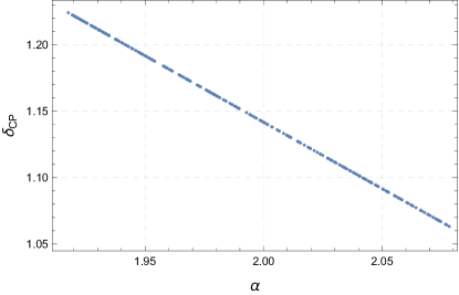
Figure 2: $\delta_{CP}$ as a function over $\alpha$ value in CKM parametrisation.

Regarding the SM charged lepton sector, we have that the third column of the SM charged lepton mass matrix arises at tree level and is given by:

$$\mathcal{M}_{i3}^{l}=y_{i3}^{(l)}\frac{v}{\sqrt{2}},$$ (82)

then implying that the third family of SM charged lepton obtains a tree level mass, while the remaining SM charged leptons get their masses at one-loop level. The entries of the first and second columns of the SM charged lepton mass matrix are generated at one loop level as shown in the Feynman diagram of Fig.(3). These entries are given by:

$$\mathcal{M}_{kn}^{l} = \mathop{\displaystyle\sum}\limits_{r=1}^{2}\frac{x_{kr}^{\left(E\right)}z_{rn}^{\left(l\right)}m_{E_{r}}}{16\pi^{2}}\left\{\sum_{i=1}^{4}R_{1i}R_{2i}f\left(m_{\rho_{i}}^{2},m_{E_{r}}^{2}\right)-\sum_{i=1}^{4}R_{3i}R_{4i}f\left(m_{\rho_{i}}^{2},m_{E_{r}}^{2}\right)\right\}$$ (84)

$$+i\mathop{\displaystyle\sum}\limits_{r=1}^{2}\frac{x_{kr}^{\left(E\right)}z_{rn}^{\left(l\right)}m_{E_{r}}}{16\pi^{2}}\left\{\sum_{i=1}^{4}R_{1i}R_{4i}f\left(m_{\rho_{i}}^{2},m_{E_{r}}^{2}\right)+\sum_{i=1}^{4}R_{2i}R_{3i}f\left(m_{\rho_{i}}^{2},m_{E_{r}}^{2}\right)\right\}.$$

Figure 3: One-loop corrections to the SM charged lepton mass matrices.

The full neutrino mass matrix in the basis $\left(\nu_{L},\nu_{R}^{c},N_{R}^{c}\right)$, has the following form:

$$\mathcal{M}_{\nu}=\left(\begin{array}[]{ccc}0_{3\times 3}&M_{\nu}^{D}&0_{3\times 2}\\ \left(M_{\nu}^{D}\right)^{T}&0_{2\times 2}&M\\ 0_{2\times 3}&M^{T}&\mu\end{array}\right),$$ (85)

where the submatrices, $M_{\nu}^{D},M$, are generated at tree level and have the following form:

$$\left(M_{\nu}\right)_{in}=\left(y_{\nu}\right)_{in}\frac{v}{\sqrt{2}},\hskip 28.45274pt\left(M\right)_{nk}=\left(y_{N}\right)_{kn}\frac{v_{\sigma}}{\sqrt{2}},$$ (86)

with $i=1,2,3$ and $k,n=1,2$. The lepton number violating Majorana neutrino mass matrix $\mu$ is obtained from the two-loop Feynman diagram in Fig.(4). The $\mu$ matrix has a similar form as the one predicted in Hernandez:2021xet ,

$$\mu_{sp} = \sum_{k=1}^{2}\frac{\left(y_{\Psi}\right)_{sn}\left(x_{\Omega}^{\ast}\right)_{nk}\left(x_{\Omega}^{{\dagger}}\right)_{kr}\left(y_{\Psi}^{T}\right)_{rp}m_{\Omega_{k}}}{4(4\pi)^{4}}\int_{0}^{1}d\alpha\int_{0}^{1-\alpha}d\beta\frac{1}{\alpha(1-\alpha)}\Biggl{[}I\left(m_{\Omega_{k}}^{2},m_{RR}^{2},m_{RI}^{2}\right)-I\left(m_{\Omega_{k}}^{2},m_{IR}^{2},m_{II}^{2}\right)\Biggr{]},$$ (87)

$$s,p,n,k,r=1,2$$

with the loop integral given by Kajiyama:2013rla :

$$I(m_{1}^{2},m_{2}^{2},m_{3}^{2})\!\!\! = \!\!\!\frac{m_{1}^{2}m_{2}^{2}\log\left(\displaystyle\frac{m_{2}^{2}}{m_{1}^{2}}\right)+m_{2}^{2}m_{3}^{2}\log\left(\displaystyle\frac{m_{3}^{2}}{m_{2}^{2}}\right)+m_{3}^{2}m_{1}^{2}\log\left(\displaystyle\frac{m_{1}^{2}}{m_{3}^{2}}\right)}{(m_{1}^{2}-m_{2}^{2})(m_{1}^{2}-m_{3}^{2})},$$

$$m_{ab}^{2}\!\!\! = \!\!\!\frac{\beta m_{\left(\varphi_{1}\right)_{a}}^{2}+\alpha m_{\left(\varphi_{3}\right)_{b}}^{2}}{\alpha(1-\alpha)}\quad(a,b=R:\mathrm{or}:I),$$ (88)

The small masses of the active neutrinos arise from an inverse seesaw mechanism at two-loop level and the mass matrices for the physical active and heavy neutrinos are respectively given by:

$$\mathcal{M}_{\text{active}}^{\nu} = M_{\nu}^{D}\left(M^{T}\right)^{-1}\mu M^{-1}\left(M_{\nu}^{D}\right)^{T},$$ (89)

$$\mathcal{M}_{\text{sterile}}^{\nu(-)} = -\frac{1}{2}\left(M+M^{T}\right)+\frac{1}{2}\mu,$$ (90)

$$\mathcal{M}_{\text{sterile}}^{\nu(+)} = \frac{1}{2}\left(M+M^{T}\right)+\frac{1}{2}\mu.$$ (91)

Due to the smallness of the $\mu$ parameter, two pairs of sterile neutrinos have a tiny mass splitting and form pseudo-Dirac pairs.

Figure 4: Two-loop Feynman diagram contributing to the $\mu$ parameter.

IV Strong CP problem

As previously mentioned, the CP symmetry is conserved in the SM sector, but explicitly broken in the dark scalar sector at tree level. The CP breaking terms can affect the Standard Model (SM) quark sector at one loop level through complex couplings of dark scalar fields. The CP-violating phase can be solely found within the CKM quark mixing matrix; however, it does not lead to a strong CP phase. No mixing terms exist between the SM and new quarks at tree or one-loop levels. Such mixing mass terms between the SM quarks and the new quarks only occur at two-loop level, as illustrated by the Feynman diagrams shown in Figs. (5), (6), (7), and (8).

Figure 5: Two-loop corrections to the SM quark mass matrices.

Figure 6: Two-loop corrections to the mixing mass matrices $\mathcal{M}_{\tilde{U}_{L}u_{R}},\mathcal{M}_{\tilde{D}_{L}d_{R}}$. Here $n=1,2$.

Figure 7: Two-loop corrections to the mixing mass matrices $\mathcal{M}_{u_{L}\tilde{U}_{R}}$. Here $i=1,2,3$ and $n,k=1,2$.

Figure 8: Two-loop corrections to the mixing mass matrices $\mathcal{M}_{d_{L}\tilde{D}_{R}}$. Here $i=1,2,3$ and $n,k=1,2$.

At the two-loop level, the mass matrices $M_{u}$ and $M_{d}$, for up and down quarks can be expressed as:

$$\mathcal{M}_{u(d)}=\mathcal{M}_{{u(d)}}^{0}+\Delta\mathcal{M}_{u(d)},$$ (92)

where

$$\Delta M_{u}=\left(\begin{array}[]{cc}\Delta\mathcal{M}_{u}&\Delta\mathcal{M}_{u_{L}\tilde{U}_{R}}\\ \Delta\mathcal{M}_{\tilde{U}_{L}u_{R}}&0\end{array}\right),\hskip 28.45274pt\Delta M_{d}=\left(\begin{array}[]{cc}\Delta\mathcal{M}_{d}&\Delta\mathcal{M}_{d_{L}\tilde{D}_{R}}\\ \Delta\mathcal{M}_{\tilde{D}_{L}d_{R}}&0\end{array}\right).$$ (93)

In the limit $m_{\tilde{U}(\tilde{D})}\gg\mathcal{M}_{u(d)}^{0}$, the SM quarks have the mass matrices given by

$$\mathcal{M}_{u} = \mathcal{M}_{u}^{0}+\Delta\mathcal{M}_{u}-\Delta\mathcal{M}_{u_{L}\tilde{U}_{R}}m_{\tilde{U}}^{-1}\Delta\mathcal{M}_{\tilde{U}_{L}u_{R}}^{T}=\mathcal{M}_{u}^{0}\left(I+M_{u}^{\epsilon}\right)\simeq\mathcal{M}_{u}^{0}e^{M_{u}^{\epsilon}},$$ (94)

$$\mathcal{M}_{d} = \mathcal{M}_{d}^{0}+\Delta\mathcal{M}_{d}-\Delta\mathcal{M}_{d_{L}\tilde{D}_{R}}m_{\tilde{D}}^{-1}\Delta\mathcal{M}_{\tilde{D}_{L}d_{R}}^{T}=\mathcal{M}_{d}^{0}\left(I+M_{d}^{\epsilon}\right)\simeq\mathcal{M}_{d}^{0}e^{M_{d}^{\epsilon}}$$ (95)

with

$$M_{u}^{\epsilon} = \left(\mathcal{M}_{u}^{0}\right)^{-1}\Delta\mathcal{M}_{u}-\left(\mathcal{M}_{u}^{0}\right)^{-1}\Delta\mathcal{M}_{u_{L}\tilde{U}_{R}}m_{\tilde{U}}^{-1}\Delta\mathcal{M}_{\tilde{U}_{L}u_{R}}^{T}\ll I,$$ (96)

$$M_{d}^{\epsilon} = \left(\mathcal{M}_{d}^{0}\right)^{-1}\Delta\mathcal{M}_{d}-\left(\mathcal{M}_{d}^{0}\right)^{-1}\Delta\mathcal{M}_{d_{L}\tilde{D}_{R}}m_{\tilde{D}}^{-1}\Delta\mathcal{M}_{\tilde{D}_{L}d_{R}}^{T}\ll I.$$ (97)

The strong CP-parameter is determined as

$$\theta = \text{Arg}|\text{Det}(\mathcal{M}_{u}\mathcal{M}_{d})|=\text{Arg}|\text{Det}(\mathcal{M}_{u}^{0}\mathcal{M}_{d}^{0}e^{(M_{u}^{\epsilon}+M_{d}^{\epsilon})})|=\text{Arg}\left|\text{Det}(\mathcal{M}_{u}^{0}\mathcal{M}_{d}^{0})e^{\text{Tr}(M_{u}^{\epsilon}+M_{d}^{\epsilon})}\right|$$ (98)

$$= \text{Arg}\left|\text{Det}(\mathcal{M}_{u}^{0}\mathcal{M}_{d}^{0})\left(1+\sum_{i=1}^{3}\left(M_{u}^{\epsilon}\right)_{ii}+\sum_{i=1}^{3}\left(M_{d}^{\epsilon}\right)_{ii})\right)\right|$$

Due to the limit, $M_{u(d)}^{\epsilon}\ll 1$ and since $\text{Arg}|(\mathcal{M}_{u}^{0}\mathcal{M}_{d}^{0})|=0$, we have

$$\theta = \Im\left|\sum_{i=1}^{3}\left(M_{u}^{\epsilon}+M_{d}^{\epsilon}\right)_{ii}\right|.$$ (99)

Notice that the two loop level corrections to $\Delta\mathcal{M}_{u},\mathcal{M}_{d}$ have opposite complex phases, similar to $\mathcal{M}_{u}^{0}$ and $\mathcal{M}_{d}^{0}$, then implying that the CP-violating parameter is determined as follows:

$$\theta\simeq\Im\left|\sum_{q=u,d}\sum_{i=1}^{3}\left(\left(\mathcal{M}_{q}^{0}\right)^{-1}\Delta\mathcal{M}_{q_{L}\tilde{U}_{R}(\tilde{D}_{R})}m_{\tilde{U}(\tilde{D})}^{-1}\Delta\mathcal{M}_{{\tilde{U}(\tilde{D}}_{L})q_{R}}^{T}\right)_{ii}\right|,$$ (100)

The quantity $\theta$ in this model is predicted to be extremely small because its effects would lead to non-zero values for $\theta$ at the four-loop level, (as follows from Eq.(100)). Notably, the two-loop corrections in the quark sectors resemble to those affecting lepton masses, particularly for Majorana-neutral leptons. As a result, the predicted values of $\theta$ are less than $\left(\frac{\text{keV}}{\text{GeV}}\right)^{2}\simeq 10^{-12}$.

V Dark matter phenomenology

After spontaneous symmetry breaking, the residual symmetry consists of two types of discrete symmetries, denoted as $Z_{2},Z_{2}^{\prime}$. Each field is associated with a pair of $(Z_{2},Z_{2}^{\prime})$ charges. Hence, the model features three types of DM classified by $(Z_{2},Z_{2}^{\prime})\in\{(0,1),(1,0),(1,1)\}$ as given in Table (5), referred to as $\text{DM}_{1,2,3}$, respectively.

If we assume that $\text{DM}_{1},\text{DM}_{2}$ are imposed to be the lightest of the fields $\text{DM}_{1,2,3}$ and $m_{\text{DM}_{3}}>m_{\text{DM}_{1}}+m_{\text{DM}_{2}}$, the model accommodates a two-component DM scenario with $\text{DM}_{1}$ and $\text{DM}_{2}$. If these conditions are not met, the model allows for three components of DM.

Now, let us explore the model with two-component DM scenario represented by $\text{DM}_{1}$ and $\text{DM}_{2}.$ In this case, we can identify two distinct scenarios for DM:

• Both DM candidates are scalars $\varphi_{3}$ and $\rho_{i}$, where $\rho_{i}$ are mixed of $\eta,\varphi_{2}$.

• One DM candidate is a scalar $\varphi_{3}$ and the other one is a fermion, $\Omega_{nR}$.

$(Z_{2},Z_{2}^{\prime})$	Fields
$\text{DM}_{1}\equiv(1,0)$	$\eta$, $\varphi_{2},\Omega_{nR}$
$\text{DM}_{2}\equiv(0,1)$	$\varphi_{3}$
$\text{DM}_{3}\equiv(1,1)$	$\varphi_{1},\Psi_{nR}$

Table 5: Three distinct kinds of dark fields determined by $Z_{2}\otimes Z_{2}^{\prime}$

First, we assume that both DM components are scalar fields, $\varphi_{3}$ and $\rho_{1}$, produced via the freeze-out mechanism. For the sake of simplicity, we consider a scenario where the scalar field $\varphi_{3}$ is mainly a weak singlet component whereas $\rho_{1}$ is mainly composed of the neutral CP even component of a $SU\left(2\right)_{L}$ electroweak doublet. Hence, $\varphi_{3}$ annihilates to normal matter only via the Higgs portal, $\rho_{1}$, whereas $\varphi_{3}$ annihilates to the SM fields via both the Higgs and gauge portals, as shown in Figs (9,10).

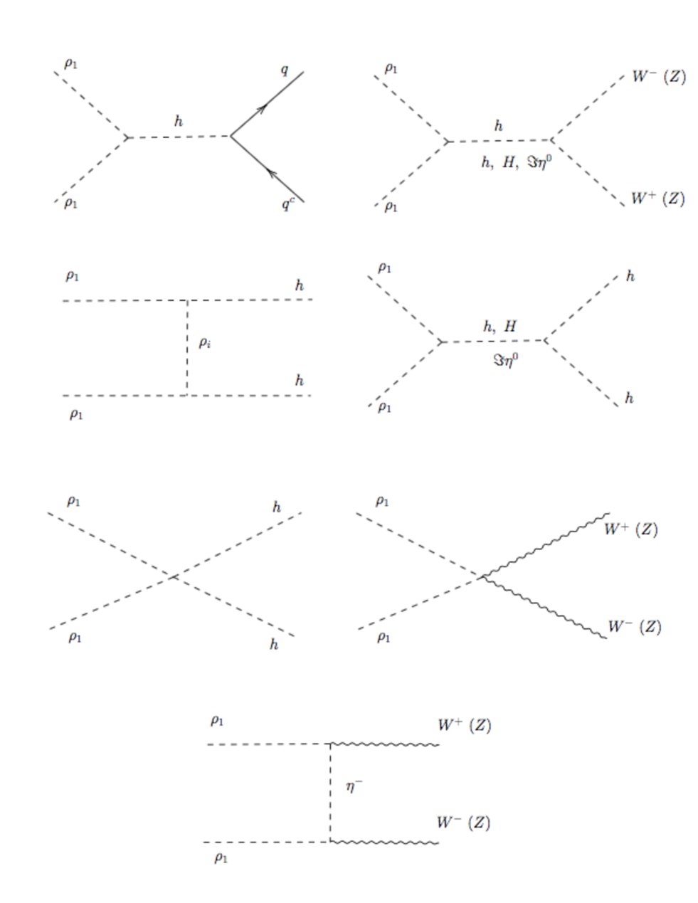
Figure 9: Annihilation of the DM, $\rho_{1}$, via a SM-like Higgs/new Higgs and gauge bosons portals

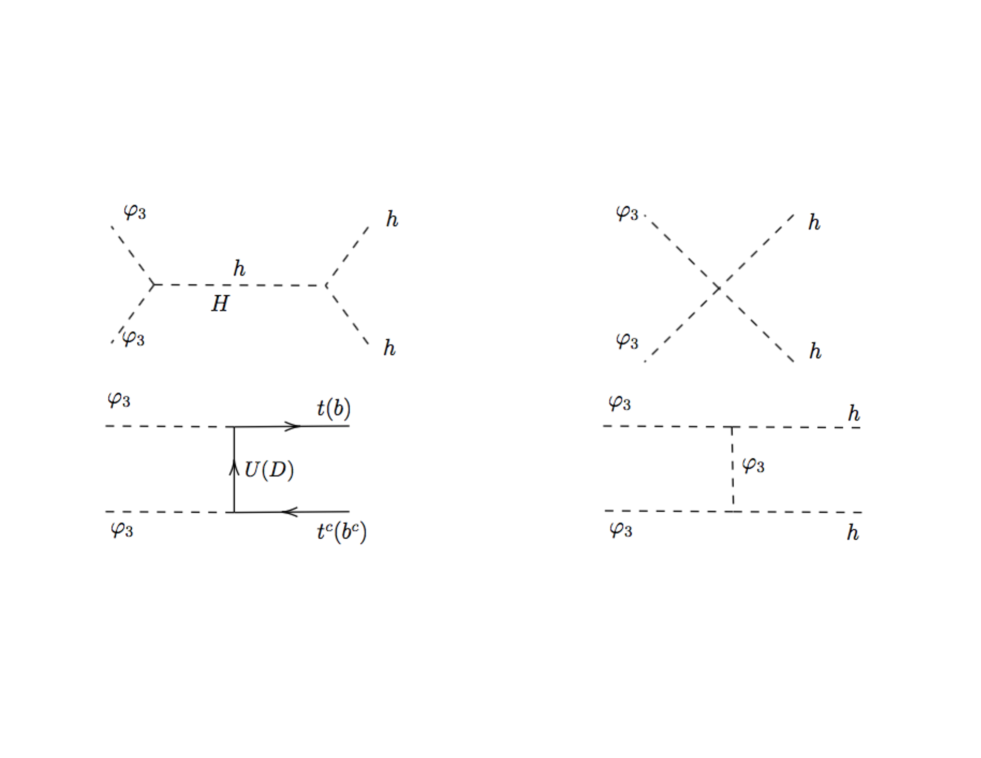
Figure 10: Annihilation of the DM, $\varphi_{3}$, via a SM-like Higgs/new Higgs portals

We assume that the DM components are lighter than other new particles, the thermally averaged annihilation cross-section times the relative velocity for

• the weak doublet, $\rho_{1}$, is approximated as

  $$<\sigma v>_{\rho_{1}\rho_{1}\rightarrow\text{SM}\text{SM}}\simeq 1\text{pb}\left\{\left(R_{11}R_{11}^{\ast}+R_{31}^{\ast}R_{31}\right)\left(\frac{600\text{GeV}}{m_{\rho_{1}}}\right)^{2}+\left(\frac{1.354\lambda_{\rho_{1}}^{\text{eff}}\text{TeV}}{m_{\rho_{1}}}\right)^{2}\right\},$$ (101)

  where the first term comes from the gauge portal whereas the last term arises from the Higgs portal, and for

• the singlet scalar, $\varphi_{3}$, is approximately given as

  $$<\sigma v>_{\varphi_{3}\varphi_{3}\to\text{SM}\text{SM}}\simeq 1\text{pb}\left(\frac{1.354\lambda^{\text{eff}}_{\varphi_{3}}\text{TeV}}{m_{\varphi_{3}}}\right)^{2},$$ (102)

  with

  $$\lambda^{\text{eff}}_{\rho_{1}} \simeq \frac{1}{2}\left(\lambda_{\sigma\eta}\sin^{2}\theta_{h}+\lambda_{\phi\varphi_{2}}\cos^{2}\theta_{h}+\lambda^{\prime}_{\phi\varphi_{2}}\cos^{2}\theta_{h}\right)\left(R_{11}R_{11}^{*}+R_{31}R_{31}^{*}\right),$$

  $$\lambda^{\text{eff}}_{\varphi_{3}} \simeq \lambda_{\sigma\varphi_{3}}\sin\theta_{h}^{2}+\lambda_{\varphi_{3}\phi}\cos\theta_{h}^{2}.$$ (103)

Furthermore, there is a conversion between two types of DM, where the heavier DM component can annihilate into the lighter one. We introduce an additional annihilation process.

$$\rho_{1}\rho_{1}\rightarrow\varphi_{3}\varphi_{3}\quad\quad if\quad m_{\rho_{1}}>m_{\varphi_{3}},$$ (104)

or

$$\varphi_{3}\varphi_{3}\rightarrow\rho_{1}\rho_{1}\quad\quad if\quad m_{\varphi_{3}}>m_{\rho_{1}},$$ (105)

The Feynman diagrams for conversion between two-component scalar DM are presented in Fig. (11).

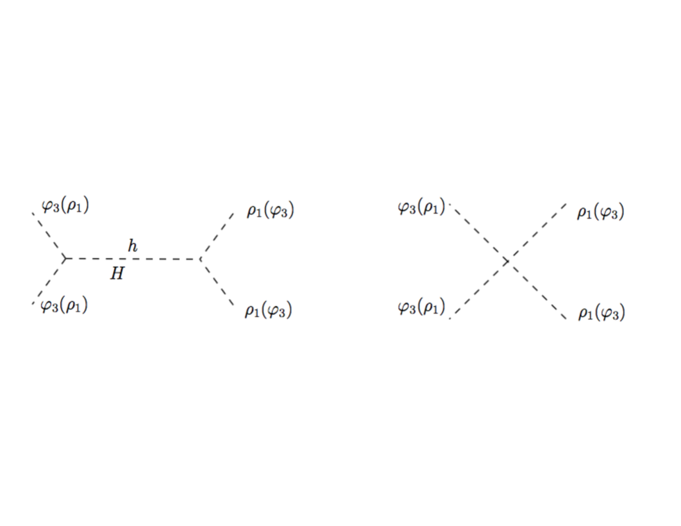
Figure 11: Conversion between two-component scalar DM.

We assume that $m_{\rho_{1}}>m_{\varphi_{3}}$. The thermally averaged annihilation cross-section times the relative velocity for conversion between two-scalar DM is approximated as follows

$$<\sigma v>_{\rho_{1}\rho_{1}\rightarrow\varphi_{3}\varphi_{3}}\simeq 1\text{pb}\sqrt{1-\frac{m_{\varphi_{3}}^{2}}{m_{\rho_{1}}^{2}}}\left(\frac{1.354\lambda_{\rho_{1}\varphi_{3}}^{\text{eff}}\text{TeV}}{m_{\rho_{1}}}\right)^{2}$$ (106)

with $\lambda_{\rho_{1}\varphi_{3}}^{\text{eff}}=\lambda_{\eta\varphi_{3}}\left(R_{11}^{\ast}R_{11}+R_{31}^{\ast}R_{31}\right)+\lambda_{\varphi_{2}\varphi_{3}}\left(R_{21}^{\ast}R_{21}+R_{41}^{\ast}R_{41}\right)$. The relic abundance for each DM component is given by

$$\Omega_{\rho_{1}}h^{2}\simeq\frac{0.1\text{pb}}{<\sigma v>_{\rho_{1}}},\quad\Omega_{\varphi_{3}}h^{2}\simeq\frac{0.1\text{pb}}{<\sigma v>_{\varphi_{3}}},$$ (107)

where

$$<\sigma v>_{\rho_{1}} = <\sigma v>_{\rho_{1}\rho_{1}\rightarrow\text{SM}\text{SM}}+<\sigma v>_{\rho_{1}\rho_{1}\rightarrow\varphi_{3}\varphi_{3}},$$

$$<\sigma v>_{\varphi_{3}} = <\sigma v>_{\varphi_{3}\varphi_{3}\rightarrow\text{SM}\text{SM}}.$$ (108)

The DM relic abundance is a sum of individual contributions as follows

$$\Omega_{\text{DM}}h^{2}=\Omega_{\rho_{1}}h^{2}+\Omega_{\varphi_{3}}h^{2}.$$ (109)

In our numerical analysis, we examine random values for the quartic scalar couplings of the portal interactions and the vacuum expectation value (VEV) for the $\sigma$ scalar field, within the ranges outlined below:

• The quadratic scalar couplings are constrained to be below their upper perturbativity bound: $\lambda_{ij}<4\pi$.

• The VEV $v_{\sigma}$ is defined within the range $100GeV<v_{\sigma}<3000GeV$ .

We establish a correlation between the relic densities of two scalar DM components and the total DM relic abundances, illustrated in Fig.(14). Additionally, we present the correlation between the masses of the two scalar DM components, shown in Fig.(13). The contributions of both scalar DM candidates depend on their respective masses. The viable mass range for dark matter compatible with the relic density extends up to the TeV scale.

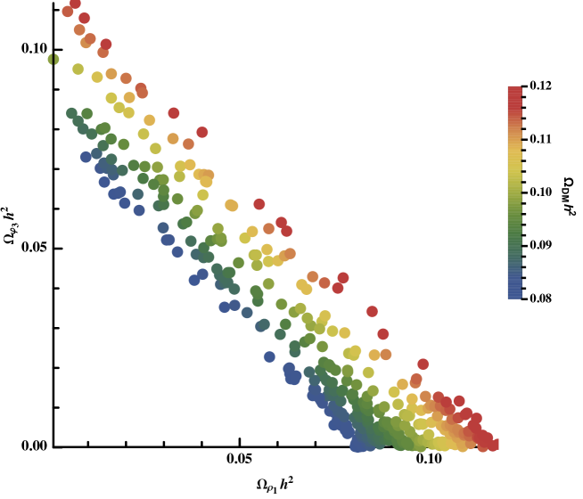
Figure 12: Correlation between the densities of two scalar dark matter components

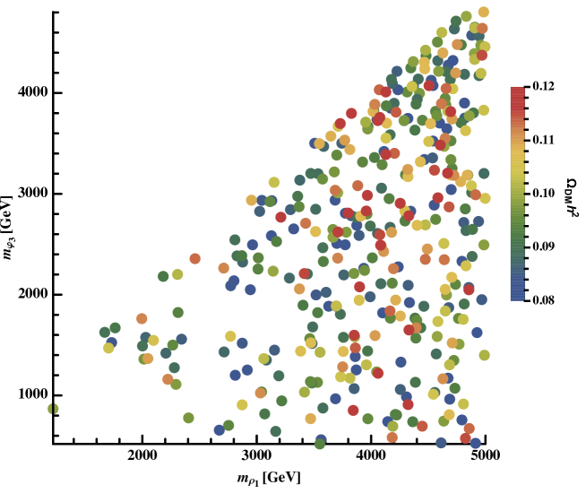
Figure 13: Correlation between the masses of two scalar dark matter components

The effective Lagrangian describing DM-nucleon interaction in the limit of zero-momentum transfer through the exchange of the Higgs boson is given as

$$\mathcal{L}_{\rho_{1},\varphi_{3}}^{eff}\simeq\frac{C_{q}^{\rho_{1}}m_{q}}{m_{\rho_{1}}^{2}}\rho_{1}\rho_{1}\bar{q}q+\frac{C_{q}^{\varphi_{3}}m_{q}}{m_{\varphi_{3}}^{2}}\varphi_{3}\varphi_{3}\bar{q}q,$$ (110)

where

$$C_{q}^{\rho_{1}}=C_{q}^{h}C_{h}^{\rho_{1}},\quad C_{q}^{\varphi_{3}}=C_{q}^{h}C_{h}^{\varphi_{3}},$$ (111)

and the coefficients, $C_{u}^{h},C_{d}^{h},C_{h}^{\varphi_{3}},C_{h}^{\rho_{1}}$, are respectively given as follows

$$C_{u_{\alpha}}^{h} = -\frac{\cos\theta_{h}}{v}\left(V_{uL}^{\ast}V_{uL}\right)_{\alpha\delta}\frac{m_{u_{\delta}}}{m_{u_{\alpha}}}\left(V_{uR}^{{\dagger}}\right)_{\delta 3}\left(V_{uR}\right)_{3\alpha},$$

$$C_{d_{\alpha}}^{h} = -\frac{\cos\theta_{h}}{v}\left(V_{dL}^{\ast}V_{dL}\right)_{\alpha\delta}\frac{m_{d_{\delta}}}{m_{d_{\alpha}}}\left(V_{dR}^{{\dagger}}\right)_{\delta 3}\left(V_{dR}\right)_{3\alpha},$$

$$C_{h}^{\varphi_{3}} = \left(\lambda_{\sigma\varphi_{3}}v_{\sigma}\sin\theta_{h}+\lambda_{\phi\varphi_{3}}v\cos\theta_{h}\right),$$

$$C_{h}^{\rho_{1}} = \frac{1}{2}\left(\lambda_{\sigma\eta}v_{\sigma}\sin\theta_{h}+\lambda_{\eta\phi}v\cos\theta_{h}+\lambda_{\eta\phi}^{\prime}v\cos\theta_{h}\right)\left(R_{11}^{\ast}R_{11}+R_{31}^{\ast}R_{31}\right)$$ (112)

$$+ \frac{1}{2}\left(\lambda_{\sigma\varphi_{2}}v_{\sigma}\sin\theta_{h}+\lambda_{\phi\varphi_{2}}v\cos\theta_{h}\right)\left(R_{21}^{\ast}R_{21}+R_{41}^{\ast}R_{41}\right).$$

The spin independent (SI) cross-section for the scattering of each DM component on a target nucleus N is expressed by

$$\sigma_{eff}^{SI}\left(\rho_{1}\right) = \frac{\Omega_{\rho_{1}}h^{2}}{\Omega_{DM}h^{2}}\sigma_{\rho_{1}N}^{SI}=\frac{\Omega_{\rho_{1}}h^{2}}{\Omega_{DM}h^{2}}\left(2\frac{m_{N\rho_{1}}}{m_{h}^{2}}\frac{m_{p}}{m_{\rho_{1}}}C_{N}^{\rho_{1}}\right)^{2},$$

$$\sigma_{eff}^{SI}\left(\varphi_{3}\right) = \frac{\Omega_{\varphi_{3}}h^{2}}{\Omega_{DM}h^{2}}\sigma_{\varphi_{3}N}^{SI}=\frac{\Omega_{\varphi_{3}}h^{2}}{\Omega_{DM}h^{2}}\left(2\frac{m_{N\varphi_{3}}}{m_{h}^{2}}\frac{m_{p}}{m_{\varphi_{3}}}C_{N}^{\varphi_{3}}\right)^{2}$$ (113)

with

$$m_{\rho_{1}(\eta_{3})N}=\frac{m_{\rho_{1}(\eta_{3})}m_{N}}{m_{\rho_{1}(\eta_{3})}+m_{N}},$$ (114)

and

$$C_{N}^{\rho_{1}(\varphi_{3})}=\frac{2}{27}\sum_{q=c,b,t}AC_{q}^{\rho_{1}(\varphi_{3})}f_{Tg}^{p}+\sum_{q=u,d,s}C_{q}^{\rho_{1}(\varphi_{3})}\left\{Zf_{Tq}^{p}+(A-Z)f_{Tq}^{n}\right\}.$$ (115)

The factors $f_{Tq}^{n}$, $f_{Tg}^{p}$, have the following values:

$$f_{Tu}^{n(p)}\simeq 0.020(0.014),\quad f_{Td}^{n(p)}\simeq 0.026(0.036),\quad f_{Ts}^{n(p)}\simeq 0.118(0.118),\quad f_{Tg}^{p}=1-\sum_{q=u,d,s}f_{Tq}^{p}.$$ (116)

We established a correlation between the spin-independent dark matter nucleon scattering cross-section and the total dark matter density in Fig. 14. Both cross-sections are predicted to align with the measurements reported in (LZ:2022lsv ).

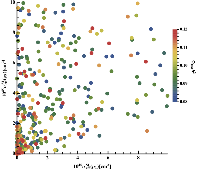
Figure 14: Correlation of the spin-independent of two DM components $(\rho_{1},\varphi_{3})$-nucleon scattering cross-section with the total DM relic abundance.

Next, we analyze a scenario involving a fermion and a scalar DM candidate. In this case, we consider $\Omega_{1R}$ and $\varphi_{3}$ as two-component DM fields. The annihilation process of the fermionic field, $\Omega_{1R}$, into SM fields is illustrated by the diagrams in Fig. (15).

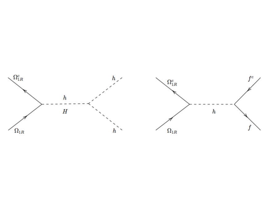
Figure 15: Annihilation of fermion DM $\Omega_{nR}$.

The conversion between fermion and scalar DM components is presented in Fig.(16), which assumes that $m_{\Omega_{1R}}>m_{\varphi_{3}}$.

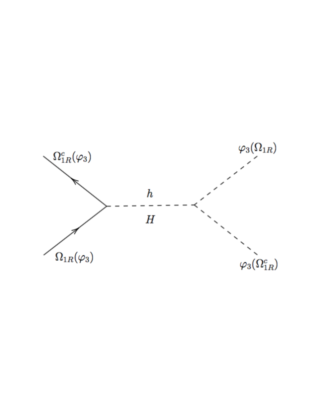
Figure 16: Conversion between fermion DM $\Omega_{nR}$ and scalar DM $\varphi_{3}$

We want to emphasize that the fermionic DM candidate $\Omega_{1R}$ interacts with the SM-like Higgs boson due to mixing $h$ with $H$. The relevant coupling strength is suppressed by $\sin^{2}\theta_{h}\simeq\frac{v^{2}}{v_{\sigma}^{2}}$. Hence, the SM-like Higgs field portal negligibly contributes to the annihilation cross-section. We expect that the s-channel mediated by the non-SM CP, even scalar $H$, will dominate the annihilation cross-section. Applying the Feynman rules, we get the thermally averaged annihilation cross-sections,

$$<v\sigma>_{\Omega_{1R}\Omega_{1R}\rightarrow SMSM} \simeq \frac{1}{8\pi}\sqrt{1-\frac{m_{h}^{2}}{m_{\Omega_{1R}}^{2}}}\left\{\frac{\lambda_{\Omega_{1R}\Omega_{1R}h}\lambda_{hhh}}{\left(4m_{\Omega_{1R}}^{2}-m_{h}^{2}\right)}+\frac{\lambda_{\Omega_{1R}\Omega_{1R}H}\lambda_{Hhh}}{\left(4m_{\Omega_{1R}}^{2}-m_{H}^{2}\right)}\right\}^{2},$$

$$<v\sigma>_{\Omega_{1R}\Omega_{1R}\rightarrow\varphi_{3}\varphi_{3}} \simeq \frac{1}{8\pi}\sqrt{1-\frac{m_{\varphi_{3}}^{2}}{m_{\Omega_{1R}}^{2}}}\left\{\frac{\lambda_{\Omega_{1R}\Omega_{1R}h}\lambda_{h\varphi_{3}\varphi_{3}}}{\left(4m_{\Omega_{1R}}^{2}-m_{h}^{2}\right)}+\frac{\lambda_{\Omega_{1R}\Omega_{1R}H}\lambda_{H\varphi_{3}\varphi_{3}}}{\left(4m_{\Omega_{1R}}^{2}-m_{H}^{2}\right)}\right\}^{2},$$ (117)

where we assume $m_{\Omega_{1R}}>m_{\varphi_{3}}$ and the couplings are determined as follows

$$\lambda_{hhh} = \frac{\lambda_{\phi}}{4}v\cos^{3}\theta_{h}-\frac{\lambda_{\sigma}}{4}v_{\sigma}\sin^{3}\theta_{h}+\frac{\lambda_{\sigma\phi}}{4}\sin 2\theta_{h}\left(-v_{\sigma}\cos\theta_{h}+v\sin\theta_{h}\right),$$

$$\lambda_{Hhh} = \frac{3}{8}\sin 2\theta_{h}\left(\lambda_{\phi}v\cos\theta_{h}+\lambda_{\sigma}v_{\sigma}\sin\theta_{h}\right)+\frac{\lambda_{\sigma\phi}}{2}\left(v_{\sigma}\cos^{3}\theta_{h}+v\sin^{3}\theta_{h}-2v\cos^{2}\theta_{h}\sin\theta_{h}-2v_{\sigma}\cos\theta_{h}\sin^{2}\theta_{h}\right),$$

$$\lambda_{\Omega_{1R}\Omega_{1R}h} \simeq -\frac{m_{\Omega_{1R}}}{2v_{\sigma}}\sin\theta_{h},\quad\lambda_{\Omega_{1R}\Omega_{1R}H}\simeq-\frac{m_{\Omega_{1R}}}{2v_{\sigma}}\cos\theta_{h},$$

$$\lambda_{h\varphi_{3}\varphi_{3}} \simeq \lambda_{\phi\varphi_{3}}v\cos\theta_{h}-\lambda_{\sigma\varphi_{3}}v_{\sigma}\sin\theta_{h},\quad\lambda_{H\varphi_{3}\varphi_{3}}\simeq\lambda_{\phi\varphi_{3}}v\sin\theta_{h}+\lambda_{\sigma\varphi_{3}}v_{\sigma}\cos\theta_{h}.$$ (118)

Moreover, in direct detection, the $\Omega_{1R}$ scatters with nucleons via only the SM-like Higgs portal due to their mixing with the new Higgs, $H$, not interacting with SM quarks and gluons. Therefore, $\Omega_{1R}$ can escape the current detection of DM.

VI $95$ GeV diphoton excess

In this section, we examine the exciting implications of our model for the $95\leavevmode\nobreak\ \text{GeV}$ diphoton excess recently reported by the CMS collaboration. We suggest that this excess in the diphoton final state, observed around $95\leavevmode\nobreak\ \text{GeV}$, could be attributed to the real component $\sigma_{R}$ of the scalar singlet $\sigma$, which we assume has a mass of $95\leavevmode\nobreak\ \text{GeV}$.

The electroweak scalar singlet $\sigma_{R}$ is primarily produced via a gluon fusion mechanism involving heavy exotic quarks $U$, $D$, $T_{n}$, and $B_{n}$ (with $n=1,2$) in a triangular loop. Its diphoton decay is mediated by triangular loops featuring the virtual exchange of vector-like quarks, charged vector-like leptons $E_{n}$ (for $n=1,2$), and electrically charged scalars. As a result, the cross-section for the production of the diphoton scalar resonance at the LHC can be represented as follows:

$$\sigma_{total}\left(pp\rightarrow\sigma_{R}\rightarrow\gamma\gamma\right)=\frac{\pi^{2}}{8}\frac{1}{m_{\sigma_{R}}\Gamma_{\sigma_{R}}}\Gamma(\sigma_{R}\rightarrow\gamma\gamma)\frac{1}{s}\int_{\frac{m_{\sigma_{R}}^{2}}{s}}^{1}\frac{dx}{x}f_{g}(x)f_{g}\left(\frac{m_{\sigma_{R}}^{2}}{sx}\right)\Gamma(\sigma_{R}\rightarrow gg),$$ (119)

where $m_{\sigma_{R}}\simeq 95\text{GeV}$ represents the mass of the resonance, and $\Gamma_{\sigma_{R}}$ denotes its total decay width. The function $f_{g}(x)$ is the gluon distribution, and $\sqrt{s}=13$ TeV is the LHC center of mass energy.

The diphoton excess observed at $95\text{ GeV}$ can be interpreted as a scalar resonance with a signal strength described by CMS:2023yay ; CMS:2024yhz ; Biekotter:2023jld :

$$\mu_{\gamma\gamma}^{\left(\exp\right)}=\frac{\sigma_{\exp}\left(pp\rightarrow\sigma_{R}\rightarrow\gamma\gamma\right)}{\sigma_{SM}\left(pp\rightarrow h\rightarrow\gamma\gamma\right)}=0.35\pm 0.12\,,$$ (120)

where $\sigma_{SM}$ corresponds to the total cross section for a hypothetical SM Higgs boson at the same mass.

The corresponding decay widths of the resonance into photon and gluon pairs are respectively given by:

$$\Gamma(\sigma_{R}\rightarrow gg)=\frac{K^{gg}\alpha_{s}^{2}m_{\sigma}^{3}}{256\pi^{3}}\left|\frac{y_{U}}{m_{U}}F(x_{U})+\frac{y_{D}}{m_{D}}F(x_{D})+\sum_{n=1}^{2}\frac{y_{T_{n}}}{m_{T_{n}}}F(x_{T_{n}})+\sum_{n=1}^{2}\frac{y_{B_{n}}}{m_{B_{n}}}F(x_{B_{n}})\right|^{2},$$ (121)

$$\Gamma(\sigma_{R}\rightarrow\gamma\gamma) = \frac{\alpha^{2}m_{\chi}^{3}}{512\pi^{3}}\left|\frac{N_{c}Q_{U}^{2}y_{U}}{m_{U}}F_{1/2}(\zeta_{U})+\frac{N_{c}Q_{D}^{2}y_{D}}{m_{D}}F_{1/2}(\zeta_{D})+\sum_{n=1}^{2}\frac{N_{c}Q_{T_{n}}^{2}y_{T_{n}}}{m_{T_{n}}}F_{1/2}(\zeta_{T_{n}})\right.$$ (122)

$$+\left.\sum_{n=1}^{2}\frac{N_{c}Q_{B_{n}}^{2}y_{B_{n}}}{m_{B_{n}}}F_{1/2}(\zeta_{B_{n}})+\mathop{\displaystyle\sum}\limits_{n=1}^{2}\frac{Q_{E_{n}}^{2}y_{E_{n}}}{m_{E_{n}}}F_{1/2}(\zeta_{E_{n}})+\frac{C_{\sigma H^{\pm}H^{\mp}}}{\sqrt{2}m_{H^{\pm}}^{2}}F_{0}(\zeta_{H^{\pm}})\right|^{2}\,,$$

where $K^{gg}\sim 1.5$ is a QCD loop enhancement factor that accounts for the higher order QCD corrections, $\zeta_{i}=4M_{i}^{2}/m_{\sigma}^{2}$, with $M_{i}=m_{U},m_{D},m_{T_{n}},m_{B_{n}},m_{E_{n}},m_{H^{\pm}}^{2}$ ($n=1,2$) and the loop functions $F_{1/2}(\zeta)$ and $F_{0}(\zeta)$ are given by:

$$F_{1/2}(\zeta)=-2\zeta\left(1+(1-\zeta)f(\zeta)\right),\,\hskip 19.91684pt\hskip 19.91684ptF_{0}(\zeta)=\left(1-\zeta f(\zeta)\right)\zeta,$$ (123)

where

$$f(\zeta)=\left\{\begin{array}[]{lcc}\left|\arcsin\sqrt{1/\zeta}\right|^{2}&\text{for}&\zeta\geq 1\\ &&\\ -\frac{1}{4}\left(\ln\left(\frac{1+\sqrt{1-\zeta}}{1-\sqrt{1-\zeta}}\right)-i\pi\right)^{2}&\text{for}&\zeta<1\\ &&\end{array}\right.$$ (124)

The Fig. (17) shows the plot of the ratio $\mu_{\gamma\gamma}$ as a function of the scalar mass $m_{H^{\pm}}$. In this plot, the masses of new exotic quarks were estimated using Eq. (56), which gives $m_{T_{1}}=m_{B_{1}}\simeq 4460$ GeV and $m_{T_{2}}=m_{B_{2}}\simeq 3858$ GeV. To evaluate the ratio $\mu_{\gamma\gamma}$, we consider $m_{U}=m_{D}\simeq 20$ TeV, $m_{E_{1}}=m_{E_{2}}\simeq 200$ GeV, and the interaction strength of $H^{\pm}H\mp\sigma$ is taken as: $C_{\sigma H^{\pm}H^{\mp}}\simeq 5$ TeV, $v_{\sigma}\simeq 5$ TeV. These values fit the ratio $\mu_{\gamma\gamma}$ at the $1\sigma$ level for the charged scalar mass in the range $950\leq m_{H^{\pm}}\leq 1800$ GeV. As indicated in Fig. (17), our model is consistent with the $95$ GeV diphoton excess.

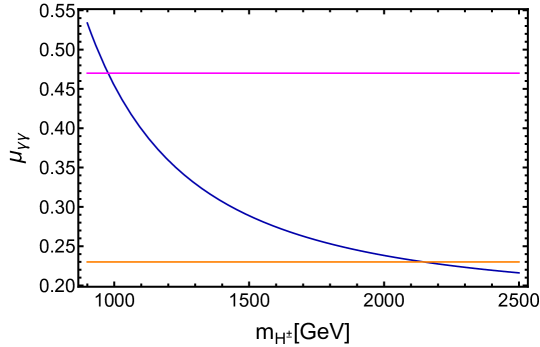
Figure 17: Signal strength for a $95GeV$ Diphoton excess as a function of the charged scalar mass $m_{H^{\pm}}$. The magenta and orange horizontal lines correspond to the $1\sigma$ upper and lower experimental bounds, respectively.

VII Charged lepton flavor violation

In this section, we will pay attention to the lepton flavor violating (LFV) decays of charged leptons. We focus in the one-loop decays $l_{i}\rightarrow l_{j}\gamma$ whose branching ratios are given by Langacker:1988up ; Lavoura:2003xp ; Hue:2017lak

$$\text{BR}\left(l_{i}\rightarrow l_{j}\gamma\right) = \frac{\alpha_{W}^{3}s_{W}^{2}m_{l_{i}}^{5}}{256\pi^{2}m_{W}^{4}\Gamma_{i}}\left|G_{ij}\right|^{2}$$ (125)

$$G_{ij} \simeq \sum_{k=1}^{3}\left(\left[\left(1-RR^{\dagger}\right)U_{\nu}\right]^{\ast}\right)_{ik}\left(\left(1-RR^{\dagger}\right)U_{\nu}\right)_{jk}G_{\gamma}\left(\frac{m_{\nu_{k}}^{2}}{m_{W}^{2}}\right)+2\sum_{l=1}^{2}\left(R^{\ast}\right)_{il}\left(R\right)_{jl}G_{\gamma}\left(\frac{m_{N_{R_{l}}}^{2}}{m_{W}^{2}}\right),$$ (126)

$$G_{\gamma}(x) = \frac{10-43x+78x^{2}-49x^{3}+18x^{3}\ln x+4x^{4}}{12\left(1-x\right)^{4}},$$

where $\Gamma_{\mu}=3\times 10^{-19}$ GeV is the total muon decay width, $U_{\nu}$ is the matrix that diagonalizes the light neutrino mass matrix which, in our case, is equal to the PMNS leptonic mixing matrix since we work on the basis where the SM-charged lepton mass matrix is diagonal. In addition, the matrix $R$ is given by

$$R=\frac{1}{\sqrt{2}}m_{D}^{\ast}M^{-1},$$ (127)

where $M$ and $m_{D}$ are the heavy Majorana mass matrix and the Dirac neutrino mass matrix, respectively.

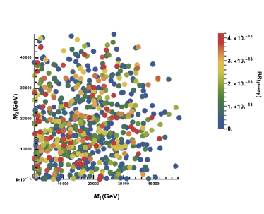
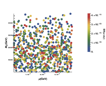
Figure 18: Correlation between $\mu\to e\gamma$ branching ratio and heavy Majorana neutrino masses, $(M_{1},M_{2})$ (panel a) and $(M_{2},\mu)$ (panel b) .

In our numerical analysis, we assume that $\mu_{1}=\mu_{2}=\mu$ and consider random heavy Majorana neutrino masses, denoted as $M_{1},M_{2},$ and $\mu$. We present the correlation between the $\mu\to e\gamma$ branching ratio and the heavy Majorana neutrino masses in two panels: panel (a) shows the relationship between $(M_{1},M_{2})$ , while panel (b) illustrates the correlation between$(M_{2},\mu)$ in Fig. 18. The model includes the allowed parameter spaces in which the predicted values for the $\mu\to e\gamma$ decay branching ratio are below the experimental upper bound MEG:2016leq and fall within the sensitivity range of future experiments.

VIII Conclusions

In summary, we have proposed an extension of the inert doublet model that successfully accommodates some of the unaddressed SM issues. This model is based on the SM gauge symmetry, supplemented by a spontaneously broken global $U(1)_{X}$ symmetry and a preserved $Z_{2}$ discrete symmetry.

In our model, the first and second families of SM-charged fermions acquire their masses through a one-loop level radiative seesaw mechanism, while the third generation of SM-charged fermions obtains their masses at tree level. The masses of the light-active neutrinos arise from a radiative inverse seesaw mechanism at two-loop level.

We successfully address the strong CP problem by preserving the CP symmetry in the SM sector’s Lagrangian at the tree level. In this approach, explicit CP violation occurs in the dark scalar sector. The CP-violating phases are then transferred to the SM quark sector at the loop level, which is crucial for providing a viable solution to the strong CP problem. We recover the CP phase in the weak sector through one-loop level corrections mediated by dark fields, while the strong CP phase emerges at the three-loop level.

The radiative nature of the seesaw mechanisms is attributed to preserved discrete symmetries, which are required for ensuring the stability of fermionic and scalar dark matter candidates. The preserved discrete symmetries also allow for multi-component dark matter, whose annihilation processes will enable us to successfully reproduce the measured amount of dark matter relic abundance while satisfying the current dark matter direct detection limits.

Additionally, the model complies with the constraints related to charged lepton flavor-violating processes, with the predicted rates for these decays falling within the current experimental sensitivity.

Finally, we interpret the 95 GeV diphoton excess reported by the CMS collaboration as a scalar resonance with a mass of 95 GeV, which aligns with the latest experimental data.

REFERENCES

- (1) A. B. McDonald, “Nobel Lecture: The Sudbury Neutrino Observatory: Observation of flavor change for solar neutrinos,” Rev.Mod.Phys. 88 (2016) 030502.
- (2) G. Bertone, D. Hooper, and J. Silk, “Particle dark matter: Evidence, candidates and constraints,” Phys. Rept. 405 (2005) 279–390, arXiv:hep-ph/0404175.
- (3) J. M. Pendlebury et al., “Revised experimental upper limit on the electric dipole moment of the neutron,” Phys. Rev. D 92 no. 9, (2015) 092003, arXiv:1509.04411 [hep-ex].
- (4) ATLAS Collaboration, G. Aad et al., “Observation of a new particle in the search for the Standard Model Higgs boson with the ATLAS detector at the LHC,” Phys. Lett. B 716 (2012) 1–29, arXiv:1207.7214 [hep-ex].
- (5) CMS Collaboration, S. Chatrchyan et al., “Observation of a New Boson at a Mass of 125 GeV with the CMS Experiment at the LHC,” Phys. Lett. B 716 (2012) 30–61, arXiv:1207.7235 [hep-ex].
- (6) CMS Collaboration, A. M. Sirunyan et al., “Observation of H production,” Phys. Rev. Lett. 120 no. 23, (2018) 231801, arXiv:1804.02610 [hep-ex].
- (7) ATLAS Collaboration, G. Aad et al., “Evidence for the Higgs-boson Yukawa coupling to tau leptons with the ATLAS detector,” JHEP 04 (2015) 117, arXiv:1501.04943 [hep-ex].
- (8) CMS Collaboration, A. M. Sirunyan et al., “Combined measurements of Higgs boson couplings in proton–proton collisions at ,” Eur. Phys. J. C 79 no. 5, (2019) 421, arXiv:1809.10733 [hep-ex].
- (9) N. Cabibbo, “Unitary symmetry and leptonic decays,” Phys. Rev. Lett. 10 (Jun, 1963) 531–533. https://link.aps.org/doi/10.1103/PhysRevLett.10.531.
- (10) CMS Collaboration, A. M. Sirunyan et al., “Observation of the Higgs boson decay to a pair of leptons with the CMS detector,” Phys. Lett. B 779 (2018) 283–316, arXiv:1708.00373 [hep-ex].
- (11) ATLAS Collaboration, M. Aaboud et al., “Observation of Higgs boson production in association with a top quark pair at the LHC with the ATLAS detector,” Phys. Lett. B 784 (2018) 173–191, arXiv:1806.00425 [hep-ex].
- (12) ATLAS Collaboration, M. Aaboud et al., “Observation of decays and production with the ATLAS detector,” Phys. Lett. B 786 (2018) 59–86, arXiv:1808.08238 [hep-ex].
- (13) B. S. Balakrishna, A. L. Kagan, and R. N. Mohapatra, “Quark Mixings and Mass Hierarchy From Radiative Corrections,” Phys. Lett. B 205 (1988) 345–352.
- (14) E. Ma, “Radiative Quark and Lepton Masses Through Soft Supersymmetry Breaking,” Phys. Rev. D 39 (1989) 1922.
- (15) T. Kitabayashi and M. Yasue, “Radiatively induced neutrino masses and oscillations in an SU(3)(L) x U(1)(N) gauge model,” Phys. Rev. D 63 (2001) 095002, arXiv:hep-ph/0010087.
- (16) D. Chang and H. N. Long, “Interesting radiative patterns of neutrino mass in an SU(3)(C) x SU(3)(L) x U(1)(X) model with right-handed neutrinos,” Phys. Rev. D 73 (2006) 053006, arXiv:hep-ph/0603098.
- (17) A. E. Carcamo Hernandez, R. Martinez, and F. Ochoa, “Radiative seesaw-type mechanism of quark masses in ,” Phys. Rev. D 87 no. 7, (2013) 075009, arXiv:1302.1757 [hep-ph].
- (18) A. E. Carcamo Hernandez, I. de Medeiros Varzielas, S. G. Kovalenko, H. Päs, and I. Schmidt, “Lepton masses and mixings in an multi-Higgs model with a radiative seesaw mechanism,” Phys. Rev. D 88 no. 7, (2013) 076014, arXiv:1307.6499 [hep-ph].
- (19) M. D. Campos, A. E. Cárcamo Hernández, S. Kovalenko, I. Schmidt, and E. Schumacher, “Fermion masses and mixings in an grand unified model with an extra flavor symmetry,” Phys. Rev. D 90 no. 1, (2014) 016006, arXiv:1403.2525 [hep-ph].
- (20) S. M. Boucenna, S. Morisi, and J. W. F. Valle, “Radiative neutrino mass in 3-3-1 scheme,” Phys. Rev. D 90 no. 1, (2014) 013005, arXiv:1405.2332 [hep-ph].
- (21) H. Okada, N. Okada, and Y. Orikasa, “Radiative seesaw mechanism in a minimal 3-3-1 model,” Phys. Rev. D 93 no. 7, (2016) 073006, arXiv:1504.01204 [hep-ph].
- (22) W. Wang and Z.-L. Han, “Radiative linear seesaw model, dark matter, and ,” Phys. Rev. D 92 (2015) 095001, arXiv:1508.00706 [hep-ph].
- (23) C. Arbeláez, A. E. Cárcamo Hernández, S. Kovalenko, and I. Schmidt, “Radiative Seesaw-type Mechanism of Fermion Masses and Non-trivial Quark Mixing,” Eur. Phys. J. C 77 no. 6, (2017) 422, arXiv:1602.03607 [hep-ph].
- (24) T. Nomura and H. Okada, “Radiatively induced Quark and Lepton Mass Model,” Phys. Lett. B 761 (2016) 190–196, arXiv:1606.09055 [hep-ph].
- (25) C. Kownacki and E. Ma, “Gauge dark symmetry and radiative light fermion masses,” Phys. Lett. B 760 (2016) 59–62, arXiv:1604.01148 [hep-ph].
- (26) T. Nomura, H. Okada, and N. Okada, “A Colored KNT Neutrino Model,” Phys. Lett. B 762 (2016) 409–414, arXiv:1608.02694 [hep-ph].
- (27) A. E. Cárcamo Hernández, J. W. F. Valle, and C. A. Vaquera-Araujo, “Simple theory for scotogenic dark matter with residual matter-parity,” Phys. Lett. B 809 (2020) 135757, arXiv:2006.06009 [hep-ph].
- (28) A. E. C. Hernández, C. Hati, S. Kovalenko, J. W. F. Valle, and C. A. Vaquera-Araujo, “Scotogenic neutrino masses with gauged matter parity and gauge coupling unification,” JHEP 03 (2022) 034, arXiv:2109.05029 [hep-ph].
- (29) A. E. Cárcamo Hernández, S. Kovalenko, F. S. Queiroz, and Y. S. Villamizar, “An extended 3-3-1 model with radiative linear seesaw mechanism,” Phys. Lett. B 829 (2022) 137082, arXiv:2105.01731 [hep-ph].
- (30) A. E. Cárcamo Hernández, V. K. N., and J. W. F. Valle, “Linear seesaw mechanism from dark sector,” JHEP 09 (2023) 046, arXiv:2305.02273 [hep-ph].
- (31) A. E. Cárcamo Hernández, Y. H. Velásquez, S. Kovalenko, N. A. Pérez-Julve, and I. Schmidt, “Models of Radiative Linear Seesaw with Electrically Charged Mediators,” PTEP 2024 no. 10, (2024) 103B02, arXiv:2403.05637 [hep-ph].
- (32) A. E. Cárcamo Hernández, I. de Medeiros Varzielas, and J. M. González, “Predictive linear seesaw model with family symmetry,” arXiv:2401.15147 [hep-ph].
- (33) A. E. Cárcamo Hernández, “A novel and economical explanation for SM fermion masses and mixings,” Eur. Phys. J. C 76 no. 9, (2016) 503, arXiv:1512.09092 [hep-ph].
- (34) J. E. Camargo-Molina, A. P. Morais, A. Ordell, R. Pasechnik, M. O. P. Sampaio, and J. Wessén, “Reviving trinification models through an E6 -extended supersymmetric GUT,” Phys. Rev. D 95 no. 7, (2017) 075031, arXiv:1610.03642 [hep-ph].
- (35) J. E. Camargo-Molina, A. P. Morais, R. Pasechnik, and J. Wessén, “On a radiative origin of the Standard Model from Trinification,” JHEP 09 (2016) 129, arXiv:1606.03492 [hep-ph].
- (36) A. E. Cárcamo Hernández and H. N. Long, “A highly predictive flavour 3-3-1 model with radiative inverse seesaw mechanism,” J. Phys. G 45 no. 4, (2018) 045001, arXiv:1705.05246 [hep-ph].
- (37) A. Dev and R. N. Mohapatra, “Natural Alignment of Quark Flavors and Radiatively Induced Quark Mixings,” Phys. Rev. D 98 no. 7, (2018) 073002, arXiv:1804.01598 [hep-ph].
- (38) A. E. Cárcamo Hernández, S. Kovalenko, J. W. F. Valle, and C. A. Vaquera-Araujo, “Neutrino predictions from a left-right symmetric flavored extension of the standard model,” JHEP 02 (2019) 065, arXiv:1811.03018 [hep-ph].
- (39) A. E. Cárcamo Hernández, S. Kovalenko, and I. Schmidt, “Radiatively generated hierarchy of lepton and quark masses,” JHEP 02 (2017) 125, arXiv:1611.09797 [hep-ph].
- (40) A. E. Cárcamo Hernández, S. Kovalenko, J. W. F. Valle, and C. A. Vaquera-Araujo, “Predictive Pati-Salam theory of fermion masses and mixing,” JHEP 07 (2017) 118, arXiv:1705.06320 [hep-ph].
- (41) A. E. Cárcamo Hernández, S. Kovalenko, H. N. Long, and I. Schmidt, “A variant of 3-3-1 model for the generation of the SM fermion mass and mixing pattern,” JHEP 07 (2018) 144, arXiv:1705.09169 [hep-ph].
- (42) A. E. Cárcamo Hernández, S. Kovalenko, R. Pasechnik, and I. Schmidt, “Sequentially loop-generated quark and lepton mass hierarchies in an extended Inert Higgs Doublet model,” JHEP 06 (2019) 056, arXiv:1901.02764 [hep-ph].
- (43) C. Arbeláez, A. E. Cárcamo Hernández, R. Cepedello, S. Kovalenko, and I. Schmidt, “Sequentially loop suppressed fermion masses from a single discrete symmetry,” JHEP 06 (2020) 043, arXiv:1911.02033 [hep-ph].
- (44) A. E. C. Hernández, S. Kovalenko, M. Maniatis, and I. Schmidt, “Fermion mass hierarchy and g 2 anomalies in an extended 3HDM Model,” JHEP 10 (2021) 036, arXiv:2104.07047 [hep-ph].
- (45) A. E. C. Hernández, D. T. Huong, and I. Schmidt, “Universal inverse seesaw mechanism as a source of the SM fermion mass hierarchy,” Eur. Phys. J. C 82 no. 1, (2022) 63, arXiv:2109.12118 [hep-ph].
- (46) V. H. Binh, C. Bonilla, A. E. Cárcamo Hernández, D. T. Huong, V. K. N., H. N. Long, P. N. Thu, and I. Schmidt, “Phenomenology of 3-3-1 models with a radiative inverse seesaw mechanism,” Phys. Rev. D 110 no. 7, (2024) 075022, arXiv:2404.13373 [hep-ph].
- (47) A. E. Cárcamo Hernández, D. T. Huong, S. Kovalenko, A. P. Morais, R. Pasechnik, and I. Schmidt, “How low-scale trinification sheds light in the flavor hierarchies, neutrino puzzle, dark matter, and leptogenesis,” Phys. Rev. D 102 no. 9, (2020) 095003, arXiv:2004.11450 [hep-ph].
- (48) A. E. Cárcamo Hernández, D. T. Huong, and H. N. Long, “Minimal model for the fermion flavor structure, mass hierarchy, dark matter, leptogenesis, and the electron and muon anomalous magnetic moments,” Phys. Rev. D 102 no. 5, (2020) 055002, arXiv:1910.12877 [hep-ph].
- (49) A. E. C. Hernández, S. F. King, and H. Lee, “Fermion mass hierarchies from vectorlike families with an extended 2HDM and a possible explanation for the electron and muon anomalous magnetic moments,” Phys. Rev. D 103 no. 11, (2021) 115024, arXiv:2101.05819 [hep-ph].
- (50) A. E. C. Hernández and I. Schmidt, “A renormalizable left-right symmetric model with low scale seesaw mechanisms,” Nucl. Phys. B 976 (2022) 115696, arXiv:2101.02718 [hep-ph].
- (51) A. E. Cárcamo Hernández, C. Espinoza, J. C. Gómez-Izquierdo, J. Marchant González, and M. Mondragón, “Phenomenology of extended multiHiggs doublet models with family symmetry,” Eur. Phys. J. C 84 no. 11, (2024) 1239, arXiv:2212.12000 [hep-ph].
- (52) A. E. Cárcamo Hernández, D. Restrepo, I. Schmidt, and O. Zapata, “Effective interactions for the SM fermion mass hierarchy and their possible UV realization,” arXiv:2308.10946 [hep-ph].
- (53) A. E. Cárcamo Hernández, K. Kowalska, H. Lee, and D. Rizzo, “Global analysis and LHC study of a vectorlike extension of the standard model with extra scalars,” Phys. Rev. D 109 no. 3, (2024) 035010, arXiv:2309.13968 [hep-ph].
- (54) P. A. C., A. E. Cárcamo Hernández, V. K. N., S. Kovalenko, R. Pasechnik, and I. Schmidt, “Left-Right model with radiative double seesaw mechanism,” JHEP 12 (2024) 162, arXiv:2405.12283 [hep-ph].
- (55) R. D. Peccei and H. R. Quinn, “Constraints Imposed by CP Conservation in the Presence of Instantons,” Phys. Rev. D 16 (1977) 1791–1797.
- (56) R. D. Peccei and H. R. Quinn, “CP Conservation in the Presence of Instantons,” Phys. Rev. Lett. 38 (1977) 1440–1443.
- (57) S. Weinberg, “A New Light Boson?,” Phys. Rev. Lett. 40 (1978) 223–226.
- (58) A. E. Nelson, “Naturally Weak CP Violation,” Phys. Lett. B 136 (1984) 387–391.
- (59) S. M. Barr, “Solving the Strong CP Problem Without the Peccei-Quinn Symmetry,” Phys. Rev. Lett. 53 (1984) 329.
- (60) A. E. Nelson, “Calculation of Barr,” Phys. Lett. B 143 (1984) 165–170.
- (61) S. M. Barr, “A Natural Class of Nonpeccei-quinn Models,” Phys. Rev. D 30 (1984) 1805.
- (62) H. B. Camara, F. R. Joaquim, and J. W. F. Valle, “Dark-sector seeded solution to the strong CP problem,” Phys. Rev. D 108 no. 9, (2023) 095003, arXiv:2303.00705 [hep-ph].
- (63) E. Ma, D. Ng, J. T. Pantaleone, and G.-G. Wong, “One Loop Induced Fermion Masses and Exotic Interactions in a Standard Model Context,” Phys. Rev. D 40 (1989) 1586.
- (64) E. Ma, “Hierarchical Radiative Quark and Lepton Mass Matrices,” Phys. Rev. Lett. 64 (1990) 2866–2869.
- (65) E. Ma, “Pathways to naturally small neutrino masses,” Phys. Rev. Lett. 81 (1998) 1171–1174, arXiv:hep-ph/9805219.
- (66) Z.-j. Tao, “Radiative seesaw mechanism at weak scale,” Phys. Rev. D 54 (1996) 5693–5697, arXiv:hep-ph/9603309.
- (67) E. Ma, “Verifiable radiative seesaw mechanism of neutrino mass and dark matter,” Phys. Rev. D 73 (2006) 077301, arXiv:hep-ph/0601225.
- (68) P.-H. Gu and U. Sarkar, “Radiative Neutrino Mass, Dark Matter and Leptogenesis,” Phys. Rev. D 77 (2008) 105031, arXiv:0712.2933 [hep-ph].
- (69) E. Ma and D. Suematsu, “Fermion Triplet Dark Matter and Radiative Neutrino Mass,” Mod. Phys. Lett. A 24 (2009) 583–589, arXiv:0809.0942 [hep-ph].
- (70) M. Hirsch, R. A. Lineros, S. Morisi, J. Palacio, N. Rojas, and J. W. F. Valle, “WIMP dark matter as radiative neutrino mass messenger,” JHEP 10 (2013) 149, arXiv:1307.8134 [hep-ph].
- (71) A. Aranda and E. Peinado, “A new radiative neutrino mass generation mechanism with higher dimensional scalar representations and custodial symmetry,” Phys. Lett. B 754 (2016) 11–13, arXiv:1508.01200 [hep-ph].
- (72) D. Restrepo, A. Rivera, M. Sánchez-Peláez, O. Zapata, and W. Tangarife, “Radiative Neutrino Masses in the Singlet-Doublet Fermion Dark Matter Model with Scalar Singlets,” Phys. Rev. D 92 no. 1, (2015) 013005, arXiv:1504.07892 [hep-ph].
- (73) R. Longas, D. Portillo, D. Restrepo, and O. Zapata, “The Inert Zee Model,” JHEP 03 (2016) 162, arXiv:1511.01873 [hep-ph].
- (74) S. Fraser, E. Ma, and M. Zakeri, “Verifiable Associated Processes from Radiative Lepton Masses with Dark Matter,” Phys. Rev. D 93 no. 11, (2016) 115019, arXiv:1511.07458 [hep-ph].
- (75) S. Fraser, C. Kownacki, E. Ma, and O. Popov, “Type II Radiative Seesaw Model of Neutrino Mass with Dark Matter,” Phys. Rev. D 93 no. 1, (2016) 013021, arXiv:1511.06375 [hep-ph].
- (76) F. von der Pahlen, G. Palacio, D. Restrepo, and O. Zapata, “Radiative Type III Seesaw Model and its collider phenomenology,” Phys. Rev. D 94 no. 3, (2016) 033005, arXiv:1605.01129 [hep-ph].
- (77) T. Nomura and H. Okada, “Loop induced type-II seesaw model and GeV dark matter with gauge symmetry,” Phys. Lett. B 774 (2017) 575–581, arXiv:1704.08581 [hep-ph].
- (78) T. Nomura and H. Okada, “Radiative neutrino mass in an alternative gauge symmetry,” Nucl. Phys. B 941 (2019) 586–599, arXiv:1705.08309 [hep-ph].
- (79) N. Bernal, A. E. Cárcamo Hernández, I. de Medeiros Varzielas, and S. Kovalenko, “Fermion masses and mixings and dark matter constraints in a model with radiative seesaw mechanism,” JHEP 05 (2018) 053, arXiv:1712.02792 [hep-ph].
- (80) W. Wang, R. Wang, Z.-L. Han, and J.-Z. Han, “The Scotogenic Models for Dirac Neutrino Masses,” Eur. Phys. J. C 77 no. 12, (2017) 889, arXiv:1705.00414 [hep-ph].
- (81) C. Bonilla, S. Centelles-Chuliá, R. Cepedello, E. Peinado, and R. Srivastava, “Dark matter stability and Dirac neutrinos using only Standard Model symmetries,” Phys. Rev. D 101 no. 3, (2020) 033011, arXiv:1812.01599 [hep-ph].
- (82) J. Calle, D. Restrepo, C. E. Yaguna, and O. Zapata, “Minimal radiative Dirac neutrino mass models,” Phys. Rev. D 99 no. 7, (2019) 075008, arXiv:1812.05523 [hep-ph].
- (83) I. M. Ávila, V. De Romeri, L. Duarte, and J. W. F. Valle, “Phenomenology of scotogenic scalar dark matter,” Eur. Phys. J. C 80 no. 10, (2020) 908, arXiv:1910.08422 [hep-ph].
- (84) A. E. Cárcamo Hernández and S. F. King, “Muon anomalies and the Yukawa relations,” Phys. Rev. D 99 no. 9, (2019) 095003, arXiv:1803.07367 [hep-ph].
- (85) C. Alvarado, C. Bonilla, J. Leite, and J. W. F. Valle, “Phenomenology of fermion dark matter as neutrino mass mediator with gauged B-L,” Phys. Lett. B 817 (2021) 136292, arXiv:2102.07216 [hep-ph].
- (86) C. Arbeláez, R. Cepedello, J. C. Helo, M. Hirsch, and S. Kovalenko, “How many 1-loop neutrino mass models are there?,” JHEP 08 (2022) 023, arXiv:2205.13063 [hep-ph].
- (87) R. Cepedello, P. Escribano, and A. Vicente, “Neutrino masses, flavor anomalies, and muon g-2 from dark loops,” Phys. Rev. D 107 no. 3, (2023) 035034, arXiv:2209.02730 [hep-ph].
- (88) J. Leite, S. Sadhukhan, and J. W. F. Valle, “Dynamical scoto-seesaw mechanism with gauged B-L symmetry,” Phys. Rev. D 109 no. 3, (2024) 035023, arXiv:2307.04840 [hep-ph].
- (89) C. Bonilla, E. Ma, E. Peinado, and J. W. F. Valle, “Two-loop Dirac neutrino mass and WIMP dark matter,” Phys. Lett. B 762 (2016) 214–218, arXiv:1607.03931 [hep-ph].
- (90) S. Baek, H. Okada, and Y. Orikasa, “A Two Loop Radiative Neutrino Model,” Nucl. Phys. B 941 (2019) 744–754, arXiv:1703.00685 [hep-ph].
- (91) S. Saad, “Origin of a two-loop neutrino mass from SU(5) grand unification,” Phys. Rev. D 99 no. 11, (2019) 115016, arXiv:1902.11254 [hep-ph].
- (92) T. Nomura and H. Okada, “A two loop induced neutrino mass model with modular symmetry,” Nucl. Phys. B 966 (2021) 115372, arXiv:1906.03927 [hep-ph].
- (93) C. Arbeláez, A. E. Cárcamo Hernández, R. Cepedello, M. Hirsch, and S. Kovalenko, “Radiative type-I seesaw neutrino masses,” Phys. Rev. D 100 no. 11, (2019) 115021, arXiv:1910.04178 [hep-ph].
- (94) S. Saad, “Combined explanations of , , anomalies in a two-loop radiative neutrino mass model,” Phys. Rev. D 102 no. 1, (2020) 015019, arXiv:2005.04352 [hep-ph].
- (95) Z.-z. Xing and D. Zhang, “On the two-loop radiative origin of the smallest neutrino mass and the associated Majorana CP phase,” Phys. Lett. B 807 (2020) 135598, arXiv:2005.05171 [hep-ph].
- (96) C.-H. Chen and T. Nomura, “Two-loop radiative seesaw, muon g 2, and -lepton-flavor violation with DM constraints,” JHEP 09 (2021) 090, arXiv:2001.07515 [hep-ph].
- (97) T. Nomura, H. Okada, and Y. Uesaka, “A two-loop induced neutrino mass model, dark matter, and LFV processes , and in a hidden local symmetry,” Nucl. Phys. B 962 (2021) 115236, arXiv:2008.02673 [hep-ph].
- (98) R. Mohapatra and J. Valle, “Neutrino Mass and Baryon Number Nonconservation in Superstring Models,” Phys. Rev. D 34 (1986) 1642.
- (99) M. Malinsky, J. C. Romao, and J. W. F. Valle, “Novel supersymmetric SO(10) seesaw mechanism,” Phys. Rev. Lett. 95 (2005) 161801, arXiv:hep-ph/0506296.
- (100) M. Malinsky, T. Ohlsson, Z.-z. Xing, and H. Zhang, “Non-unitary neutrino mixing and CP violation in the minimal inverse seesaw model,” Phys. Lett. B 679 (2009) 242–248, arXiv:0905.2889 [hep-ph].
- (101) A. Abada and M. Lucente, “Looking for the minimal inverse seesaw realisation,” Nucl. Phys. B 885 (2014) 651–678, arXiv:1401.1507 [hep-ph].
- (102) S. Mandal, N. Rojas, R. Srivastava, and J. W. F. Valle, “Dark matter as the origin of neutrino mass in the inverse seesaw mechanism,” Phys. Lett. B 821 (2021) 136609, arXiv:1907.07728 [hep-ph].
- (103) A. Abada, N. Bernal, A. E. C. Hernández, X. Marcano, and G. Piazza, “Gauged inverse seesaw from dark matter,” Eur. Phys. J. C 81 no. 8, (2021) 758, arXiv:2107.02803 [hep-ph].
- (104) A. E. C. Hernández, C. Espinoza, J. C. Gómez-Izquierdo, and M. Mondragón, “Fermion masses and mixings, dark matter, leptogenesis and muon anomaly in an extended 2HDM with inverse seesaw,” Eur. Phys. J. Plus 137 no. 11, (2022) 1224, arXiv:2104.02730 [hep-ph].
- (105) C. Bonilla, A. E. Carcamo Hernandez, B. Saez Dıaz, S. Kovalenko, and J. Marchant Gonzalez, “Dark matter from a radiative inverse seesaw majoron model,” Phys. Lett. B 847 (2023) 138282, arXiv:2306.08453 [hep-ph].
- (106) C. Bonilla, A. E. Carcamo Hernandez, S. Kovalenko, H. Lee, R. Pasechnik, and I. Schmidt, “Fermion mass hierarchy in an extended left-right symmetric model,” JHEP 12 (2023) 075, arXiv:2305.11967 [hep-ph].
- (107) A. Abada, N. Bernal, A. E. Cárcamo Hernández, S. Kovalenko, and T. B. de Melo, “Three-Loop Inverse Scotogenic Seesaw Models,” arXiv:2312.14105 [hep-ph].
- (108) Y. Kajiyama, H. Okada, and T. Toma, “Multicomponent dark matter particles in a two-loop neutrino model,” Phys. Rev. D 88 no. 1, (2013) 015029, arXiv:1303.7356 [hep-ph].
- (109) LZ Collaboration, J. Aalbers et al., “First Dark Matter Search Results from the LUX-ZEPLIN (LZ) Experiment,” Phys. Rev. Lett. 131 no. 4, (2023) 041002, arXiv:2207.03764 [hep-ex].
- (110) CMS Collaboration, “Search for a standard model-like Higgs boson in the mass range between 70 and 110 in the diphoton final state in proton-proton collisions at ,”.
- (111) CMS Collaboration, A. Hayrapetyan et al., “Search for a standard model-like Higgs boson in the mass range between 70 and 110 GeV in the diphoton final state in proton-proton collisions at = 13 TeV,” arXiv:2405.18149 [hep-ex].
- (112) T. Biekötter, S. Heinemeyer, and G. Weiglein, “The CMS di-photon excess at 95 GeV in view of the LHC Run 2 results,” Phys. Lett. B 846 (2023) 138217, arXiv:2303.12018 [hep-ph].
- (113) P. Langacker and D. London, “Lepton Number Violation and Massless Nonorthogonal Neutrinos,” Phys. Rev. D 38 (1988) 907.
- (114) L. Lavoura, “General formulae for ,” Eur. Phys. J. C 29 (2003) 191–195, arXiv:hep-ph/0302221.
- (115) L. T. Hue, L. D. Ninh, T. T. Thuc, and N. T. T. Dat, “Exact one-loop results for in 3-3-1 models,” Eur. Phys. J. C 78 no. 2, (2018) 128, arXiv:1708.09723 [hep-ph].
- (116) MEG Collaboration, A. M. Baldini et al., “Search for the lepton flavour violating decay with the full dataset of the MEG experiment,” Eur. Phys. J. C 76 no. 8, (2016) 434, arXiv:1605.05081 [hep-ex].