Supplemental Information

S-I Correspondence between dynamical systems and multilayered neural networks

In preparation for discussing the DFA-adjoint method for continuous-time dynamical systems with time delay, we summarize the relationship between the adjoint optimal control method for dynamical systems and backpropagation used for training traditional multilayered neural networks (NNs).

S-I.1 Backpropagation

First, we consider an ordinary fully connected multilayered NN, where the output in the $n$-th layer, $\mbox{\boldmath$z$}_{n+1}\in\mathbb{R}^{M_{n+1}}$, is expressed as follows:

$$\mbox{\boldmath$z$}_{n+1}=\mbox{\boldmath$F$}_{n}({\bm{a}}_{n}),$$ (S1)

$${\bm{a}}_{n}={\bm{W}}^{(n)}\mbox{\boldmath$z$}_{n},$$ (S2)

where $M_{n+1}$ represents the number of nodes in the $n+1$-th layer, $\mbox{\boldmath$F$}_{n}$ represents an activation function, and ${\bm{W}}^{(n)}$ represents a weight matrix of the $n$th layer. The $L$ dimensional target vector ${\bm{y}}_{\mathrm{tag}}$ and the output from the last layer ${\bm{y}}=\mbox{\boldmath$G$}_{\mathrm{out}}(\mbox{\boldmath$z$}_{N},{\bm{w}})\in\mathbb{R}^{L}$ determine the loss function $L({\bm{y}},{\bm{y}}_{\mathrm{tag}})$, where $\mbox{\boldmath$G$}_{\mathrm{out}}$ represents an activation function for the output layer. We assume that the loss function $L$ and $\mbox{\boldmath$G$}_{\mathrm{out}}$ are the mean squared error (MSE) and an identity function for a regression task, respectively, whereas $L$ and $\mbox{\boldmath$G$}_{\mathrm{out}}$ are the cross entropy and softmax function for a classification task, respectively. To minimize $L({\bm{y}},{\bm{y}}_{\mathrm{tag}})$, the weights should be optimized according to the following gradient (row) vector:

$$\frac{\text{d}L}{\text{d}{{\bm{W}}^{(n)}}} =\frac{\partial L}{\partial\mbox{\boldmath$z$}_{n+1}}\frac{\text{d}\mbox{\boldmath$z$}_{n+1}}{\text{d}{{\bm{W}}^{(n)}}}=\frac{\partial L}{\partial\mbox{\boldmath$z$}_{n+1}}\frac{\partial\mbox{\boldmath$F$}_{n}}{\partial{{\bm{W}}^{(n)}}}.$$ (S3)

The gradient (row) vector ${\partial L}/{\partial\mbox{\boldmath$z$}_{n}}$ is computed backward from $\frac{\partial L}{\partial\mbox{\boldmath$z$}_{N}}$ in the last layer, using the following equation recurrently:

$$\frac{\partial L}{\partial\mbox{\boldmath$z$}_{n}}=\frac{\partial L}{\partial\mbox{\boldmath$z$}_{n+1}}\frac{\partial\mbox{\boldmath$z$}_{n+1}}{\partial\mbox{\boldmath$z$}_{n}}=\frac{\partial L}{\partial\mbox{\boldmath$z$}_{n+1}}\frac{\partial\mbox{\boldmath$F$}_{n}}{\partial\mbox{\boldmath$z$}_{n}}.$$ (S4)

Here, if ${\partial L}/{\partial\mbox{\boldmath$z$}_{n}}$ is defined by ${\bm{p}}^{\mathrm{T}}_{n}$ as follows:

$${\bm{p}}^{\mathrm{T}}_{n}=\frac{\partial L}{\partial\mbox{\boldmath$z$}_{n}},$$ (S5)

where ^T represents transpose, Eq. (S4) is rewritten as follows:

$${\bm{p}}^{\mathrm{T}}_{n}={\bm{p}}^{\mathrm{T}}_{n+1}\frac{\partial\mbox{\boldmath$F$}_{n}}{\partial\mbox{\boldmath$z$}_{n}}.$$ (S6)

Owing to the definition of ${\bm{a}}_{n}={\bm{W}}^{(n)}\mbox{\boldmath$z$}_{n}$, ${\bm{p}}^{\mathrm{T}}_{n}$ has the following relationship with the error to be back-propagated, ${\bm{e}}^{\mathrm{T}}_{n}={\partial L}/{\partial{\bm{a}}_{n}}$,

$${\bm{p}}^{\mathrm{T}}_{n}=\frac{\partial L}{\partial\mbox{\boldmath$z$}_{n}}=\frac{\partial L}{\partial{\bm{a}}_{n}}\frac{\partial{\bm{a}}_{n}}{\partial\mbox{\boldmath$z$}_{n}}={\bm{e}}_{n}^{\mathrm{T}}{\bm{W}}^{(n)}.$$ (S7)

Considering Eq. (S7), Eq. (S6) is rewritten as follows:

$${\bm{e}}_{n}^{\mathrm{T}}={\bm{e}}^{\mathrm{T}}_{n+1}{\bm{W}}^{(n+1)}\frac{\partial\mbox{\boldmath$F$}_{n}}{\partial{\bm{a}}_{n}}.$$ (S8)

Hence, the gradient of $L$ with respect to the element $W_{ij}^{(n)}$ of the weight matrix ${\bm{W}}^{(n)}$ is expressed as follows:

$$\dfrac{dL}{dW_{ij}^{(n)}}={\bm{e}}_{n+1}^{\mathrm{T}}{\bm{W}}^{(n+1)}\dfrac{\partial\mbox{\boldmath$F$}_{n}}{\partial W_{ij}^{(n)}}.$$ (S9)

In the gradient descent method for training, the update of the weight matrix is expressed such that $\delta W_{ij}^{(n)}\propto-{dL}/{dW_{ij}^{(n)}}$. Hence, the update $\delta W_{ij}^{(n)}$ can be computed by solving Eqs. (S8) and (S9).

When considering the output in the multilayered NN, $\mbox{\boldmath$z$}_{n}$, as the dynamical variable ($N_{r}$ dimensional system state vector) of a discrete-time dynamical system, the layer-to-layer information propagation in the NN is expressed as the time-evolution of the dynamical system governed by a nonlinear function $\mathbf{F}_{n}$. The time evolution of the discrete-time dynamical system can be expressed as follows:

$${\bm{r}}_{n+1}=\mbox{\boldmath$F$}_{n}({\bm{r}}_{n},\mbox{\boldmath$u$}_{n}),$$ (S10)

where ${\bm{r}}_{n}\in\mathbb{R}^{N_{r}}$ and $\mbox{\boldmath$u$}_{n}\in\mathbb{R}^{N_{u}}$ represent the system state vector and tuning parameter vector at the $n$-th time step, respectively. The input data ${\bm{x}}$ is encoded as ${\bm{r}}_{0}=\mbox{\boldmath$G$}_{\mathrm{in}}({\bm{x}})$, and the final state ${\bm{r}}_{N}$ after $N$ steps is used to generate an output ${\bm{y}}=\mbox{\boldmath$G$}_{\mathrm{out}}({\bm{r}}_{N},{\bm{w}})$, where $\mbox{\boldmath$G$}_{\mathrm{in}}$ and $\mbox{\boldmath$G$}_{\mathrm{out}}$ are functions required to convert between input/output data and the system state vector in the input and output processes, respectively. ${\bm{w}}$ denotes the weight parameters of the output function. The loss function is defined as $L({\bm{y}},{\bm{y}}_{\mathrm{tag}})$. By minimizing $L({\bm{y}},{\bm{y}}_{\mathrm{tag}})$ through optimization of the parameters $\mbox{\boldmath$u$}_{n}$ and ${\bm{w}}$, the dynamical system performs as effectively as the multilayered NN.

If ${\bm{p}}_{n}$ is defined as

$${\bm{p}}_{n}^{\mathrm{T}}=\frac{\partial L}{\partial{\bm{r}}_{n}},$$ (S11)

the gradient vector for the optimization is expressed as,

$$\frac{\text{d}L}{\text{d}\mbox{\boldmath$u$}_{n}} =\frac{\partial L}{\partial{\bm{r}}_{n+1}}\frac{\text{d}{\bm{r}}_{n+1}}{\text{d}\mbox{\boldmath$u$}_{n}}=\frac{\partial L}{\partial{\bm{r}}_{n+1}}\frac{\partial\mbox{\boldmath$F$}_{n}}{\partial\mbox{\boldmath$u$}_{n}}$$

$$={\bm{p}}_{n+1}^{\mathrm{T}}\frac{\partial\mbox{\boldmath$F$}_{n}}{\partial\mbox{\boldmath$u$}_{n}}.$$ (S12)

The vector ${\bm{p}}_{n}$ can be computed backward from the final state ${\bm{p}}_{N}$ using the following equation recurrently:

$${\bm{p}}_{n}^{\mathrm{T}} =\frac{\partial L}{\partial{\bm{r}}_{n}}=\frac{\partial L}{\partial{\bm{r}}_{n+1}}\frac{\partial\mbox{\boldmath$F$}_{n}}{\partial{\bm{r}}_{n}}$$

$$={\bm{p}}_{n+1}^{\mathrm{T}}\frac{\partial\mbox{\boldmath$F$}_{n}}{\partial{\bm{r}}_{n}}.$$ (S13)

Thus, the update $\delta\mbox{\boldmath$u$}^{\mathrm{T}}_{n}\propto-{\text{d}L}/{\text{d}\mbox{\boldmath$u$}_{n}}$ can be computed by solving Eqs. (S12) and (S13). As shown in Sec. S-II, ${\bm{p}}_{n}$ corresponds to the adjoint vector, and Eq. (S13) corresponds to the adjoint equation, which can be used for the optimal control of a discrete-time dynamical system.

S-I.2 Direct feedback alignment (DFA)

In the DFA method for multilayered NNs, the error vector ${\bm{e}}_{n}$ and weight matrix ${\bm{W}}^{(n+1)}$ are replaced with the error at the last layer ${\bm{e}}={\partial L}/{\partial{\bm{a}}_{N}}\in\mathbb{R}^{L}$ and a random matrix ${\bm{B}}_{n}\in\mathbb{R}^{L\times N_{r}}$, respectively. Considering Eq. (S7), ${\bm{p}}_{n}$ is replaced by

$$\hat{{\bm{p}}}^{\mathrm{T}}_{n}={\bm{e}}^{\mathrm{T}}{\bm{B}}_{n}.$$ (S14)

The error ${\bm{e}}$ is given by ${\bm{y}}-{\bm{y}}_{\mathrm{tag}}$ when the loss function $L$ is the MSE for a regression task as $L=1/2({\bm{y}}-{\bm{y}}_{\mathrm{tag}})^{2}$ or the cross entropy for a classification task as $L=-{\bm{y}}_{\mathrm{tag}}\log{\bm{y}}$.

With this expression, the matrix element $\hat{W}_{ij}^{(n)}$ is updated as follows:

$$\delta\hat{W}_{ij}^{(n)} \propto-{\bm{e}}^{\mathrm{T}}{\bm{B}}_{n+1}\dfrac{\partial\mbox{\boldmath$F$}_{n}}{\partial W_{ij}^{(n)}}.$$ (S15)

When applying this scheme for multilayered NNs directly into the dynamical system, the vector ${\bm{p}}_{n}^{\mathrm{T}}$ outlined in Eq. (S11) can be replaced by

$$\hat{{\bm{p}}}_{n}^{\mathrm{T}}={\bm{e}}^{\mathrm{T}}{\bm{B}}_{n}.$$ (S16)

Hence, $\hat{{\bm{u}}}^{(n)}$ is updated as follows:

$$\delta\hat{{\bm{u}}}_{n}^{\mathrm{T}}\propto-\hat{{\bm{p}}}_{n+1}^{\mathrm{T}}\frac{\partial\mbox{\boldmath$F$}_{n}}{\partial{\bm{u}}_{n}}=-{\bm{e}}^{\mathrm{T}}{\bm{B}}_{n+1}\frac{\partial\mbox{\boldmath$F$}_{n}}{\partial{\bm{u}}_{n}}.$$ (S17)

S-II Adjoint equations for discrete time dynamical systems

Here, we apply the adjoint method developed for optimal control of dynamical systems to Eq. (S10) and obtain the adjoint equations. The derived adjoint equation and gradient vector correspond to Eq. (S13) for backpropagation and Eq. (S12), respectively. Derivation proceeds by first incorporating the constraint of Eq. (S10) into an augmented loss function $L_{\mathrm{aug}}$ with the Lagrangian multiplier vector, ${\bm{p}}_{n}\in{\mathbb{R}}^{N_{r}}$. The augmented loss function is given as

$$L_{\mathrm{aug}}=L({\bm{y}},{\bm{y}}_{\mathrm{tag}})+\sum_{n=0}^{N-1}{\bm{p}}^{\mathrm{T}}_{n+1}\left(\mbox{\boldmath$F$}_{n}-{\bm{r}}_{n+1}\right).$$ (S18)

Notably, $L_{\mathrm{aug}}=L({\bm{y}},{\bm{y}}_{\mathrm{tag}})$ for all valid trajectories of ${\bm{r}}_{n}$ obeying Eq. (S10). The second term of Eq. (S18) can be rewritten as follows:

$$\sum_{n=0}^{N-1}{\bm{p}}^{\mathrm{T}}_{n+1}\left(\mbox{\boldmath$F$}_{n}-{\bm{r}}_{n+1}\right)=\sum_{n=0}^{N-1}{\bm{p}}^{\mathrm{T}}_{n+1}\mbox{\boldmath$F$}_{n}-\sum_{n=1}^{N}{\bm{p}}^{\mathrm{T}}_{n}{\bm{r}}_{n}=\sum_{n=1}^{N-1}\left({\bm{p}}^{\mathrm{T}}_{n+1}\mbox{\boldmath$F$}_{n}-{\bm{p}}^{\mathrm{T}}_{n}{\bm{r}}_{n}\right)+{\bm{p}}^{\mathrm{T}}_{1}{\bm{r}}_{0}-{\bm{p}}^{\mathrm{T}}_{N}{\bm{r}}_{N},$$ (S19)

and we have,

$$L_{\mathrm{aug}} =L+\sum_{n=1}^{N-1}\left({\bm{p}}^{\mathrm{T}}_{n+1}\mbox{\boldmath$F$}_{n}-{\bm{p}}^{\mathrm{T}}_{n}{\bm{r}}_{n}\right)+{\bm{p}}^{\mathrm{T}}_{1}{\bm{r}}_{0}-{\bm{p}}^{\mathrm{T}}_{N}{\bm{r}}_{N}.$$ (S20)

The gradient vector is computed as follows:

$$\frac{\text{d}L}{\text{d}{\bm{u}}_{n}}=\frac{\text{d}L_{\mathrm{aug}}}{\text{d}{\bm{u}}_{n}} =\frac{\partial L}{\partial{\bm{r}}_{N}}\frac{\text{d}{\bm{r}}_{N}}{\text{d}{\bm{u}}_{n}}+\sum_{n^{\prime}=1}^{N-1}{\bm{p}}^{\mathrm{T}}_{n^{\prime}+1}\left(\frac{\partial\mbox{\boldmath$F$}_{n^{\prime}}}{\partial{\bm{r}}_{n^{\prime}}}\frac{\text{d}{\bm{r}}_{n^{\prime}}}{\text{d}{\bm{u}}_{n}}+\frac{\partial\mbox{\boldmath$F$}_{n^{\prime}}}{\partial{\bm{u}}_{n}}\right)-\sum_{n^{\prime}=1}^{N-1}{\bm{p}}^{\mathrm{T}}_{n^{\prime}}\frac{\text{d}{\bm{r}}_{n^{\prime}}}{\text{d}{\bm{u}}_{n}}-{\bm{p}}^{\mathrm{T}}_{N}\frac{\text{d}{\bm{r}}_{N}}{\text{d}{\bm{u}}_{n}}$$

$$=\left(\frac{\partial L}{\partial{\bm{r}}_{N}}-{\bm{p}}_{N}^{\mathrm{T}}\right)\frac{\text{d}{\bm{r}}_{N}}{\text{d}{\bm{u}}_{n}}+\sum_{n^{\prime}=1}^{N-1}\left({\bm{p}}_{n^{\prime}+1}^{\mathrm{T}}\frac{\partial\mbox{\boldmath$F$}_{n^{\prime}}}{\partial{\bm{r}}_{n^{\prime}}}-{\bm{p}}_{n^{\prime}}^{\mathrm{T}}\right)\frac{\text{d}{\bm{r}}_{n^{\prime}}}{\text{d}{\bm{u}}_{n}}+\sum_{n^{\prime}=1}^{N-1}{\bm{p}}^{\mathrm{T}}_{n^{\prime}+1}\frac{\partial\mbox{\boldmath$F$}_{n^{\prime}}}{\partial{\bm{u}}_{n}}$$

$$=\left(\frac{\partial L}{\partial{\bm{r}}_{N}}-{\bm{p}}_{N}^{\mathrm{T}}\right)\frac{\text{d}{\bm{r}}_{N}}{\text{d}{\bm{u}}_{n}}+\sum_{n^{\prime}=1}^{N-1}\left({\bm{p}}_{n^{\prime}+1}^{\mathrm{T}}\frac{\partial\mbox{\boldmath$F$}_{n^{\prime}}}{\partial{\bm{r}}_{n^{\prime}}}-{\bm{p}}_{n^{\prime}}^{\mathrm{T}}\right)\frac{\text{d}{\bm{r}}_{n^{\prime}}}{\text{d}{\bm{u}}_{n}}+{\bm{p}}^{\mathrm{T}}_{n+1}\frac{\partial\mbox{\boldmath$F$}_{n}}{\partial{\bm{u}}_{n}},$$ (S21)

where ${\text{d}{\bm{r}}_{0}}/{\text{d}{\bm{u}}_{n}}=0$ is utilized because the initial state ${\bm{r}}_{0}$ is independent on ${\bm{u}}_{n}$. In addition, the third term is derived from ${\partial\mbox{\boldmath$F$}_{n^{\prime}}}/{\partial{\bm{u}}_{n}}={\partial\mbox{\boldmath$F$}_{n}}/{\partial{\bm{u}}_{n}}\delta_{n^{\prime}n}{}$, where $\delta_{n^{\prime}n}$ denotes the Kronecker’s delta.

The Lagrangian multiplier ${\bm{p}}_{n}$ can be set freely; therefore, we can select ${\bm{p}}_{n}$ such that it satisfies the following equations:

$${\bm{p}}^{\mathrm{T}}_{N}=\frac{\partial L}{\partial{\bm{r}}_{N}},$$ (S22)

and

$${\bm{p}}^{\mathrm{T}}_{n}={\bm{p}}^{\mathrm{T}}_{n+1}\frac{\partial\mbox{\boldmath$F$}_{n}}{\partial{\bm{r}}_{n}},$$ (S23)

for $n\in\{1,\cdots,N-1\}$. This results in a simple form of ${\text{d}L_{\mathrm{aug}}}/{\text{d}{\bm{u}}_{n}}$ as,

$$\frac{\text{d}L_{\mathrm{aug}}}{\text{d}{\bm{u}}_{n}}={\bm{p}}^{\mathrm{T}}_{n+1}\frac{\partial\mbox{\boldmath$F$}_{n}}{\partial{\bm{u}}_{n}}.$$ (S24)

Because ${\text{d}L}/{\text{d}{\bm{u}}_{n}}={\text{d}L_{\mathrm{aug}}}/{\text{d}{\bm{u}}_{n}}$ in the gradient descent scheme, the update $\delta{\bm{u}}_{n}$ is given as,

$$\delta{\bm{u}}^{\mathrm{T}}_{n}\propto-{\bm{p}}^{\mathrm{T}}_{n+1}\frac{\partial\mbox{\boldmath$F$}_{n}}{\partial{\bm{u}}_{n}}.$$ (S25)

In summary, when we set the adjoint vector ${\bm{p}}_{n}$ such that it satisfies Eqs. (S22) and (S23), the adjoint Eq. (S23) corresponds to backward Eq. (S13), suggesting ${\bm{p}}^{\mathrm{T}}_{n}={\partial L}/{\partial{\bm{r}}_{n}}$; thus, we can obtain the same update equation as Eq. (S12).

S-II.1 DFA for adjoint method in discrete-time dynamical systems

In this subsection, we describe the DFA-based training for the adjoint method, based on the correspondence between backpropagation and the adjoint method. Concretely, the adjoint vector ${\bm{p}}_{n}$ is replaced by $\hat{{\bm{p}}}^{\mathrm{T}}_{n}={\bm{e}}^{\mathrm{T}}{\bm{B}}_{n}$, where ${\bm{e}}={\bm{y}}-{\bm{y}}_{\mathrm{tag}}$ and ${\bm{B}}_{n}$ denote the error vector in the last layer and a random matrix, respectively. By substituting this into Eq.(S25), the update rule based on the DFA scheme is given as follows:

$$\delta\hat{{\bm{u}}}_{n}^{\mathrm{T}} \propto-\hat{{\bm{p}}}_{n+1}^{\mathrm{T}}\frac{\partial\mbox{\boldmath$F$}_{n}}{\partial{\bm{u}}_{n}}$$

$$=-{\bm{e}}^{\mathrm{T}}{\bm{B}}_{n+1}\frac{\partial\mbox{\boldmath$F$}_{n}}{\partial{\bm{u}}_{n}}.$$ (S26)

We call this training method and the vector $\hat{{\bm{p}}}$ as DFA–adjoint method and DFA–adjoint vector, respectively.

S-III Adjoint equations for continuous-time dynamical systems

We consider a continuous-time dynamical system. It is assumed that the system state ${\bm{r}}(t)\in\mathbb{R}^{N_{r}}$ can be controlled by continuously altering the control vector ${\bm{u}}(t)\in\mathbb{R}^{N_{u}}$ and is governed by the following equation:

$$\frac{\text{d}{\bm{r}}(t)}{\text{d}t}=\mbox{\boldmath$F$}[{\bm{r}}(t),{\bm{u}}(t)].$$ (S27)

The system state ${\bm{r}}(t)$ evolves starting from an initial state synthesized from input ${\bm{x}}$ as ${\bm{r}}(0)=\mbox{\boldmath$G$}_{\mathrm{in}}({\bm{x}})$. The input information is transformed through the time evolution up to time $t=T_{e}$. The output vector ${\bm{y}}\in\mathbb{R}^{L}$ is given with the final state ${\bm{r}}(T_{e})$ as ${\bm{y}}=\mbox{\boldmath$G$}_{\mathrm{out}}[{\bm{r}}(T_{e})]$. The learning process aims at optimizing the control signal ${\bm{u}}(t)$ such that the loss function $L({\bm{y}},{\bm{y}}_{\mathrm{tag}})$ is minimized for a given training dataset.

The augmented loss function $L_{\mathrm{aug}}$ with the Lagrangian multiplier (adjoint) vector ${\bm{p}}(t)$ is given as

$$L_{\mathrm{aug}}=L({\bm{y}},{\bm{y}}_{\mathrm{tag}})+\int_{0}^{T_{e}}{\bm{p}}^{\mathrm{T}}(t)\left\{\mbox{\boldmath$F$}[{\bm{r}}(t),{\bm{u}}(t)]-\frac{\text{d}{\bm{r}}(t)}{\text{d}t}\right\}dt.$$ (S28)

The second term of the aforementioned equation can be rewritten as

$$\int_{0}^{T_{e}}{\bm{p}}^{\mathrm{T}}(t)\left(\mbox{\boldmath$F$}({\bm{r}},{\bm{u}})-\frac{\text{d}{\bm{r}}(t)}{\text{d}t}\right)dt=-\left[{\bm{p}}^{\mathrm{T}}(t){\bm{r}}(t)\right]_{0}^{T_{e}}+\int_{0}^{T_{e}}\left({\bm{p}}^{\mathrm{T}}(t)\mbox{\boldmath$F$}({\bm{r}},{\bm{u}})+\frac{\text{d}{{\bm{p}}}^{\mathrm{T}}(t)}{\text{d}t}{\bm{r}}(t)\right)dt,$$ (S29)

and the augmented loss function $L_{\mathrm{aug}}$ is as follows:

$$L_{\mathrm{aug}}=L({\bm{y}},{\bm{y}}_{\mathrm{tag}})-{\bm{p}}^{\mathrm{T}}(T_{e}){\bm{r}}(T_{e})+{\bm{p}}^{\mathrm{T}}(0){\bm{r}}(0)+\int_{0}^{T_{e}}\left({\bm{p}}^{\mathrm{T}}(t)\mbox{\boldmath$F$}({\bm{r}},{\bm{u}})+\frac{\text{d}{{\bm{p}}}^{\mathrm{T}}(t)}{\text{d}t}{\bm{r}}(t)\right)dt.$$ (S30)

In terms of variations $\delta L$ and $\delta{\bm{r}}(t)$ with respect to $\delta{\bm{u}}(t)$, we can obtain,

$$\delta L_{\mathrm{aug}} =\left\{\frac{\partial L}{\partial{\bm{r}}(T_{e})}-{\bm{p}}^{\mathrm{T}}(T_{e})\right\}\delta{{\bm{r}}(T_{e})}+\int_{0}^{T_{e}}\left\{{\bm{p}}^{\mathrm{T}}(t)\frac{\partial\mbox{\boldmath$F$}}{\partial{\bm{r}}}+\frac{\text{d}{\bm{p}}^{\mathrm{T}}}{\text{d}t}\right\}\delta{\bm{r}}(t)dt+\int_{0}^{T_{e}}{\bm{p}}^{\mathrm{T}}(t)\frac{\partial\mbox{\boldmath$F$}}{\partial{\bm{u}}}\delta{\bm{u}}(t)dt,$$ (S31)

where $\delta{\bm{r}}(0)=0$ is used because we assume that ${\bm{r}}(0)=\mbox{\boldmath$G$}_{\mathrm{in}}({\bm{x}})$ is fixed in this case. When we choose ${\bm{p}}(t)$ such that ${\bm{p}}^{\mathrm{T}}(T_{e})={\partial L}/{\partial{\bm{r}}(T_{e})}$ and the following equation is satisfied,

$$\frac{\text{d}{\bm{p}}^{\mathrm{T}}(t)}{\text{d}t}=-{\bm{p}}^{\mathrm{T}}(t)\frac{\partial\mbox{\boldmath$F$}}{\partial{\bm{r}}},$$ (S32)

$L_{\mathrm{aug}}$ is simplified as $\int_{0}^{T_{e}}{\bm{p}}^{\mathrm{T}}(t){\partial\mbox{\boldmath$F$}}/{\partial{\bm{u}}}\delta{\bm{u}}(t)dt$. Accordingly, $\delta L_{\mathrm{aug}}\leq 0$ when we can choose $\delta{\bm{u}}(t)$ as

$$\delta{\bm{u}}^{\mathrm{T}}(t)\propto-{\bm{p}}^{\mathrm{T}}(t)\frac{\partial\mbox{\boldmath$F$}}{\partial{\bm{u}}}.$$ (S33)

S-III.1 DFA–adjoint for continuous-time dynamical systems

Similar to the DFA–adjoint in discrete-time systems, the connection with the DFA method in continuous-time systems is made by replacing the adjoint vector ${\bm{p}}^{\mathrm{T}}(t)$ with the DFA–adjoint vector $\hat{{\bm{p}}}^{\mathrm{T}}(t)$. This vector is defined as

$$\hat{{\bm{p}}}^{\mathrm{T}}(t)={\bm{e}}^{T}{\bm{B}}(t),$$ (S34)

where ${\bm{e}}={\bm{y}}-{\bm{y}}_{\mathrm{tag}}\in\mathbb{R}^{L}$ and ${\bm{B}}(t)\in\mathbb{R}^{L\times N_{r}}$ denote the error vector in the last layer and a time-dependent matrix, respectively. We assume that the time variation of ${\bm{B}}(t)$ is not limited to random in continuous-time systems, unlike the conventional DFA method. In Sec. S-V, we set ${\bm{B}}(t)$ as a various time-dependent function and evaluated the performance. Because the control signal ${\bm{u}}(t)$ is dependent on ${\bm{B}}(t)$ via $\hat{{\bm{p}}}(t)$, the characteristic timescale of ${\bm{B}}(t)$ should be close to that of the dynamical system.

The DFA–adjoint method can be applied to arbitrary continuous-time dynamical systems. Given the equivalence between multilayered NNs and dynamical systems, utilizing high-dimensional dynamical systems is crucial for achieving optimal performance. However, finding high-dimensional dynamical systems with numerous controllable parameters for physical implementations poses a significant challenge. To address this issue, we introduce a dynamical system with a time delay in the subsequent section.

S-IV Adjoint equations for continuous-time systems with time delay

In dynamical systems with time delay, the degrees of freedom in the time domain can be exploited as virtual nodes, which can be leveraged for computational purposes. Consequently, physical systems with time delay are useful for facilitating large-scale computations even with a simple physical configuration. In this section, we delve into the dynamical systems with time delay and derive the adjoint equation [Eq. (2) in the main text] and the update rule for the control signal ${\bm{u}}(t)$. Additionally, we also derive the update rule for the static system parameter ${\bm{\theta}}$ and input mask ${\bm{m}}(t)$ for a more general formulation.

To this end, we begin with the following $N_{r}$ dimensional equation,

$$\frac{\text{d}{\bm{r}}(t)}{\text{d}t}=\mbox{\boldmath$F$}\left[{\bm{r}}(t),{\bm{r}}(t-\tau_{D}),{\bm{u}}(t),{\bm{\theta}}\right].$$ (S35)

We assumed that the input ${\bm{x}}\in\mathbb{R}^{N_{x}}$ is encoded by a matrix ${\bm{m}}(t)\in\mathbb{R}^{N_{x}\times N_{r}}$ as follows:

$${\bm{r}}(t)=\mbox{\boldmath$G$}_{\mathrm{in}}({\bm{x}},t)={\bm{m}}^{\mathrm{T}}(t){\bm{x}},\mbox{ for $-\tau_{D}\leq t\leq 0$},$$ (S36)

and the output ${\bm{y}}\in\mathbb{R}^{L}$ is given by

$${\bm{y}}=\mbox{\boldmath$G$}_{\mathrm{out}}({\bm{z}}),$$ (S37)

$${\bm{z}}=\int_{T_{e}-T_{c}}^{T_{e}}{\bm{w}}(t){\bm{r}}(t)dt,$$ (S38)

where ${\bm{w}}(t)\in\mathbb{R}^{L\times N_{r}}$ represents an weight matrix to produce the output, and $T_{c}$ represents the time length to extract the output from the time series.

The augmented loss function is given by

$$L_{\mathrm{aug}}=L\left[{\bm{y}}_{\mathrm{tag}},{\bm{y}}\left({\bm{z}}\right)\right]+\int_{0}^{T_{e}}{\bm{p}}^{\mathrm{T}}(t)\left\{\mbox{\boldmath$F$}[{\bm{r}},{\bm{r}}(t-\tau_{D}),{\bm{u}},{\bm{\theta}}]-\frac{\text{d}{\bm{r}}(t)}{\text{d}t}\right\}dt.$$ (S39)

Because the second term of the aforementioned equation can be rewritten as

$$\int_{0}^{T_{e}}{\bm{p}}^{\mathrm{T}}(t)\left(\mbox{\boldmath$F$}-\frac{\text{d}{\bm{r}}(t)}{\text{d}t}\right)dt=-\left[{\bm{p}}^{\mathrm{T}}(t){\bm{r}}(t)\right]_{0}^{T_{e}}+\int_{0}^{T_{e}}\left({\bm{p}}^{\mathrm{T}}(t)\mbox{\boldmath$F$}+\frac{\text{d}{{\bm{p}}^{\mathrm{T}}}(t)}{\text{d}t}{\bm{r}}(t)\right)dt,$$ (S40)

the variations $\delta L_{\mathrm{aug}}$ and $\delta{\bm{r}}(t)$ in terms of $\delta{\bm{u}}(t)$, $\delta{\bm{\theta}}$, and $\delta{\bm{m}}(t)$ can be derived as follows:

$$\delta L_{\mathrm{aug}} =\frac{\partial L}{\partial{\bm{z}}}\delta{\bm{z}}-\left\{{\bm{p}}^{\mathrm{T}}(0)\delta{\bm{r}}(0)-{\bm{p}}^{\mathrm{T}}(T_{e})\delta{\bm{r}}(T_{e})\right\}+\int_{0}^{T_{e}}\left(\frac{\text{d}{{\bm{p}}}^{\mathrm{T}}}{\text{d}t}+{\bm{p}}^{\mathrm{T}}\frac{\partial\mbox{\boldmath$F$}}{\partial{\bm{r}}}\right)\delta{\bm{r}}dt$$

$$+\int_{0}^{T_{e}}{\bm{p}}^{\mathrm{T}}(t)\frac{\partial\mbox{\boldmath$F$}}{\partial{\bm{r}}_{\tau_{D}}}\delta{\bm{r}}_{\tau_{D}}dt+\int_{0}^{T_{e}}{\bm{p}}^{\mathrm{T}}\frac{\partial\mbox{\boldmath$F$}}{\partial{\bm{u}}}\delta{\bm{u}}dt+\int_{0}^{T_{e}}{\bm{p}}^{\mathrm{T}}\frac{\partial\mbox{\boldmath$F$}}{\partial{\bm{\theta}}}\delta{\bm{\theta}}dt,$$ (S41)

where ${\bm{r}}_{\tau_{D}}={\bm{r}}(t-\tau_{D})$ and

$$\delta{\bm{z}}=\int_{T_{e}-T_{c}}^{T_{e}}{\bm{w}}(t)\delta{\bm{r}}dt=\int_{0}^{T_{e}}\Theta_{1}(t){\bm{w}}(t)\delta{\bm{r}}dt.$$ (S42)

$\Theta_{1}(t)$ represents the indicator function, which equals 1 for $T_{e}-T_{c}\leq t\leq T_{e}$ and 0 otherwise. The third term in Eq. (S41) can be rewritten as follows:

$$\int_{0}^{T_{e}}{\bm{p}}^{\mathrm{T}}\frac{\partial\mbox{\boldmath$F$}}{\partial{\bm{r}}_{\tau_{D}}}\delta{\bm{r}}_{\tau_{D}}dt =\int_{-\tau_{D}}^{T_{e}-\tau_{D}}{\bm{p}}^{\mathrm{T}}(t+\tau_{D})\frac{\partial\mbox{\boldmath$F$}(t+\tau_{D})}{\partial{\bm{r}}}\delta{\bm{r}}dt$$

$$=\int_{0}^{T_{e}}\Theta_{0}(t){\bm{p}}^{\mathrm{T}}(t+\tau_{D})\frac{\partial\mbox{\boldmath$F$}(t+\tau_{D})}{\partial{\bm{r}}}\delta{\bm{r}}dt+\int_{-\tau_{D}}^{0}{\bm{p}}^{\mathrm{T}}(t+\tau_{D})\frac{\partial\mbox{\boldmath$F$}(t+\tau_{D})}{\partial{\bm{r}}}\delta{\bm{r}}dt,$$ (S43)

where $\Theta_{0}(t)$ represents the indicator function, which equals 1 for $0<t\leq T_{e}-\tau_{D}$ and 0 otherwise. Therefore, the augmented loss function is rewritten as

$$\delta L_{\mathrm{aug}}= -{\bm{p}}^{\mathrm{T}}(T_{e})\delta{\bm{r}}(T_{e})$$

$$+\int_{0}^{T_{e}}\left[\Theta_{1}(t)\frac{\partial L}{\partial{\bm{z}}}{\bm{w}}+\frac{\text{d}{{\bm{p}}}^{\mathrm{T}}}{\text{d}t}+{\bm{p}}^{\mathrm{T}}\frac{\partial\mbox{\boldmath$F$}}{\partial{\bm{r}}}+\Theta_{0}(t){\bm{p}}^{\mathrm{T}}(t+\tau_{D})\frac{\partial\mbox{\boldmath$F$}(t+\tau_{D})}{\partial{\bm{r}}}\right]\delta{\bm{r}}dt$$

$$+\int_{0}^{T_{e}}{\bm{p}}^{\mathrm{T}}\frac{\partial\mbox{\boldmath$F$}}{\partial{\bm{u}}}\delta{\bm{u}}dt+\int_{0}^{T_{e}}{\bm{p}}^{\mathrm{T}}\frac{\partial\mbox{\boldmath$F$}}{\partial{\bm{\theta}}}\delta{\bm{\theta}}dt+\int_{-\tau_{D}}^{0}{\bm{p}}^{\mathrm{T}}(t+\tau_{D})\frac{\partial\mbox{\boldmath$F$}(t+\tau_{D})}{\partial{\bm{r}}}\delta{\bm{m}}^{\mathrm{T}}{\bm{x}}dt.$$ (S44)

We can choose the adjoint vector ${\bm{p}}(t)$ such that the following equation is satisfied:

$$\frac{\text{d}{\bm{p}}^{\mathrm{T}}}{\text{d}t}=-\Theta_{1}(t)\frac{\partial L}{\partial{\bm{z}}}{\bm{w}}-{\bm{p}}^{\mathrm{T}}\frac{\partial\mbox{\boldmath$F$}}{\partial{\bm{r}}}-\Theta_{0}(t){\bm{p}}^{\mathrm{T}}(t+\tau_{D})\frac{\partial\mbox{\boldmath$F$}(t+\tau_{D})}{\partial{\bm{r}}}.$$ (S45)

In this case, the variation in the loss function is

$$\delta L_{\mathrm{aug}}=\int_{0}^{T_{e}}{\bm{p}}^{\mathrm{T}}\frac{\partial\mbox{\boldmath$F$}}{\partial{\bm{u}}}\delta{\bm{u}}dt+\left(\int_{0}^{T_{e}}{\bm{p}}^{\mathrm{T}}\frac{\partial\mbox{\boldmath$F$}}{\partial{\bm{\theta}}}dt\right)\delta{\bm{\theta}}+\int_{-\tau_{D}}^{0}{\bm{p}}^{\mathrm{T}}(t+\tau_{D})\frac{\partial\mbox{\boldmath$F$}(t+\tau_{D})}{\partial{\bm{r}}}\delta{\bm{m}}^{\mathrm{T}}{\bm{x}}dt.$$ (S46)

Accordingly, we can obtain $\delta L_{\mathrm{aug}}\leq 0$ if ${\bm{u}}(t)$, ${\bm{\theta}}$, and ${\bm{m}}(t)$ are updated as follows:

$$\delta{\bm{u}}(t) =-\alpha_{u}\left({\bm{p}}^{\mathrm{T}}\frac{\partial\mbox{\boldmath$F$}}{\partial{\bm{u}}}\right)^{\mathrm{T}}$$ (S47)

$$\delta{\bm{\theta}} =-\alpha_{\theta}\int_{0}^{T_{e}}\left({\bm{p}}^{\mathrm{T}}\frac{\partial\mbox{\boldmath$F$}}{\partial{\bm{\theta}}}\right)^{\mathrm{T}}dt$$ (S48)

$$\delta{\bm{m}}^{\mathrm{T}}(t) =-\alpha_{m}\left[{\bm{p}}^{\mathrm{T}}(t+\tau_{D})\frac{\partial\mbox{\boldmath$F$}(t+\tau_{D})}{\partial{\bm{r}}}\right]^{\mathrm{T}}{\bm{x}}^{\mathrm{T}},$$ (S49)

where $\alpha_{u}$, $\alpha_{\theta}$, and $\alpha_{m}$ are positive constant values. ${\bm{u}}(t)$, ${\bm{\theta}}$, and ${\bm{m}}^{\mathrm{T}}(t)$ can be updated based on these update rules by solving the adjoint Eq. (S45). Instead of solving the adjoint equation, we can set

$$\hat{{\bm{p}}}^{\mathrm{T}}(t)={\bm{e}}^{\mathrm{T}}{\bm{B}}(t).$$ (S50)

The update rules based on the DFA–adjoint method are expressed as follows:

$$\delta{\bm{u}}(t) =-\alpha_{u}\left({\bm{B}}(t)\frac{\partial\mbox{\boldmath$F$}}{\partial{\bm{u}}}\right)^{\mathrm{T}}{\bm{e}}$$ (S51)

$$\delta{\bm{\theta}} =-\alpha_{\theta}\int_{0}^{T_{e}}\left({\bm{B}}(t)\frac{\partial\mbox{\boldmath$F$}}{\partial{\bm{\theta}}}\right)^{\mathrm{T}}{\bm{e}}dt$$ (S52)

$$\delta{\bm{m}}^{\mathrm{T}}(t) =-\alpha_{m}\left[{\bm{B}}(t+\tau_{D})\frac{\partial\mbox{\boldmath$F$}(t+\tau_{D})}{\partial{\bm{r}}}\right]^{\mathrm{T}}{\bm{e}}{\bm{x}}^{\mathrm{T}}.$$ (S53)

S-V Time-dependent random matrix ${\bm{B}}(t)$

In this section, we set various time-dependent random matrices ${\bm{B}}(t)$ and evaluated the classification accuracy for the MNIST handwritten digit image dataset under different scenarios [Fig. S1]. In three distinct cases, the elements $B_{li}(t)$ of the time-dependent random matrix were generated using uniformly distributed random numbers within $\left[0,1\right]$, normally distributed random numbers with zero mean and unit variance, and binary random numbers $\{-1,1\}$, such that $B_{li}$ satisfies $\langle(B_{li}(t)-\bar{B})(B_{l^{\prime}i^{\prime}}(t^{\prime})-\bar{B})\rangle_{t}=\sigma^{2}\delta(t-t^{\prime})\delta_{ll^{\prime}}\delta_{ii^{\prime}}$, where $\bar{B}$ and $\sigma^{2}$ represent the mean and variance, respectively. $l$ and $i$ denote the indices of a target class and the degree of freedom of ${\bm{r}}(t)$, respectively. In addition, we introduced a periodic waveform defined as $B_{li}(t)=B^{0}_{li}\sin(\omega t+2\pi l/10)$ and explored the performance for various angular frequencies. Notably, we determined that, when $2\pi/\omega=85.03$ $\mu$s is close to the timescale $\tau_{L}$, the classification accuracy reached 0.94.

We used the following ${\bm{B}}(t)$ in the main text,

$$B_{li}=\sum_{m=1}^{M_{B}}A_{m}^{(li)}\sin\left(\omega_{m}t+2\pi\phi_{m}^{(li)}\right),$$ (S54)

and we obtained an accuracy of more than 0.97, surpassing the performance of the other configurations. Here, $A_{m}^{(li)}$ and $\phi_{m}^{(li)}$ are random numbers sampled from the continuous uniform distribution within $[0,1)$. The angular frequencies were determined by $\omega_{m}=2\pi(14m/M_{B}+1)$, where the unit for the angular frequency is radian per millisecond. $M_{B}=3\times 28^{2}$ was used.

Figure S2 shows the classification accuracy as a function of $M_{B}$ in Eq. (S54). For $M_{B}\geq 4$, the accuracy was saturated to be approximately 97$\%$.

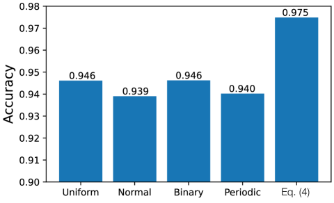
Figure S1: Classification accuracy for the MNIST handwritten digit dataset. The time series of ${\bm{B}}(t)$ was set as uniformly distributed random numbers (Uniform) within $\left[0,1\right]$, normally distributed random numbers (Normal), binary random numbers (Binary), a periodic waveform with a period of 85.03 $\mu$s (Periodic), and the waveform shown in Eq. (4) in the main text.

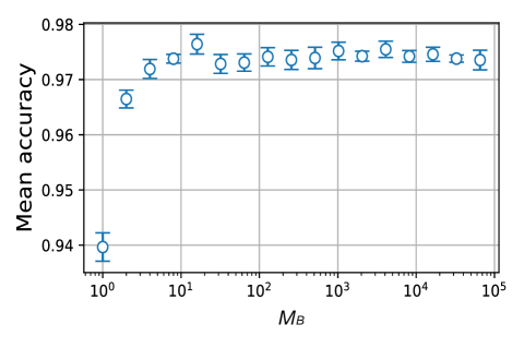
Figure S2: Classification accuracy as a function of $M_{B}$.

S-VI Toward a model-free training approach

The drawback of the DFA–adjoint method is the requirement of detailed prior knowledge of dynamical operator $F$ in the physical system. For example, ${\partial\mbox{\boldmath$F$}}/{\partial{\bm{u}}}$ is used for the update of control ${\bm{u}}$, as shown in Eq. (S51). This may make it difficult to use the DFA–adjoint method for training the system. To address this issue, we introduce two different approaches in this section.

S-VI.1 Augmented DFA–adjoint method

We assume that we do not possess an accurate model of the physical system, $\dot{{\bm{r}}}=\mbox{\boldmath$F$}({\bm{r}},{\bm{r}}(t-\tau_{D}),{\bm{u}})$; instead, we have an approximate model, represented as $\dot{{\bm{r}}}\approx\mbox{\boldmath$H$}({\bm{r}},{\bm{r}}(t-\tau_{D}),{\bm{u}})$. In this case, we can use $\mbox{\boldmath$H$}({\bm{r}},{\bm{r}}(t-\tau_{D}),{\bm{u}})$ to compute the derivatives required for the update in Eqs. (S51)–(S53) instead of using $\mbox{\boldmath$F$}({\bm{r}},{\bm{r}}(t-\tau_{D}),{\bm{u}})$. In this method, ${\bm{u}}$ is updated as follows:

$${\bm{u}}(t)\rightarrow{\bm{u}}(t)-\alpha_{u}\delta{\bm{u}}_{aug}(t),$$ (S55)

where

$$\delta{\bm{u}}_{aug}(t) =-\alpha_{u}\left({\bm{B}}(t)\frac{\partial\mbox{\boldmath$H$}}{\partial{\bm{u}}}\right)^{\mathrm{T}}{\bm{e}}.$$ (S56)

If the physical system depends on parameter ${\bm{\theta}}$, we use the model $\mbox{\boldmath$H$}({\bm{r}},{\bm{r}}(t-\tau_{D}),{\bm{u}},{\bm{\theta}})$. When the parameter ${\bm{\theta}}$ and mask pattern ${\bm{m}}(t)$ are also trained, the updates $\delta{\bm{\theta}}_{aug}$ and $\delta{\bm{m}}_{aug}(t)$ are expressed as follows:

$$\delta{\bm{\theta}}_{aug} =-\alpha_{\theta}\int_{0}^{T_{e}}\left({\bm{B}}(t)\frac{\partial\mbox{\boldmath$H$}}{\partial{\bm{\theta}}}\right)^{\mathrm{T}}{\bm{e}}dt$$ (S57)

$$\delta{\bm{m}}^{\mathrm{T}}_{aug}(t) =-\alpha_{m}\left[{\bm{B}}(t+\tau_{D})\frac{\partial\mbox{\boldmath$H$}(t+\tau_{D})}{\partial{\bm{r}}}\right]^{\mathrm{T}}{\bm{e}}{\bm{x}}^{\mathrm{T}}.$$ (S58)

This method is inspired by the so-called augmented DFA [10], where the derivatives of the activation function in a neural network are replaced with an appropriate function that correlates with the original activation function. In this sense, we refer to the proposed method as the augmented DFA–adjoint method in this study. The augmented DFA–adjoint method is more general than the augmented DFA because it can be applied to a wide range of physical systems where neurons and synaptic weights cannot be explicitly defined.

Table S1 presents the classification accuracy achieved with the augmented DFA–adjoint method, using the Gaussian, $\tanh$, and Softplus (a smooth approximation of ReLU) functions as $H$. These functions are typically used as activation functions in conventional neural networks but differ from the original $F$. The factors, ${\bm{a}}_{0}$, ${\bm{a}}_{1}$, and ${\bm{a}}_{2}$, are used to compensate for the timescale of the system and learning rate. We found that the augmented DFA–adjoint method with the Gaussian and $\tanh$ models achieves classification accuracy close to that of the DFA–adjoint method. In the case of the Softplus function model ($\log(1+e^{\delta})$), the accuracy degraded to approximately 91$\%$, but this is still better than that achieved with the ELM. These results suggest that a precise model of the physical system is not necessary; an approximate model of $F$ is sufficient for training. This may be attributed to the error robustness of the proposed approach, as discussed in the main text.

Table S1: Comparison of classification accuracy between the DFA–adjoint and augmented DFA–adjoint methods using $\mbox{\boldmath$H$}=\pm{\bm{a}}_{0}\exp(-\delta^{2})$, ${\bm{a}}_{1}\tanh(\delta+\pi/4)$, and ${\bm{a}}_{2}\log(1+e^{\delta})$. $\delta=u_{1}(t)r_{1}(t-\tau_{D})+u_{2}(t)$, ${\bm{a}}_{0}=(1/\tau_{L},1/\tau_{L})^{\mathrm{T}}$, ${\bm{a}}_{1}=(1/\tau_{L},1/\tau_{L})^{\mathrm{T}}/10$, ${\bm{a}}_{2}=(1/\tau_{L},1/\tau_{L})/10^{4}$. The MNIST dataset was used for this comparison.

Methods	Model	Accuracy
DFA–adjoint	Eqs. (S66) and (S67)	$0.973$
Augmented DFA–adjoint	${\bm{a}}_{0}\exp(-\delta^{2})$	$0.970$
Augmented DFA–adjoint	$-{\bm{a}}_{0}\exp(-\delta^{2})$	$0.970$
Augmented DFA–adjoint	${\bm{a}}_{1}\tanh(\delta+\pi/4)$	$0.967$
Augmented DFA–adjoint	${\bm{a}}_{2}\log(1+e^{\delta})$	$0.906$
ELM (w/o control)	-	$0.869$

S-VI.2 Additive control-based DFA–adjoint method

The proposed DFA–adjoint method is based on an external control approach. Thus, we can flexibly design how to apply control signal ${\bm{u}}(t)$ to the physical system, so that ${\bm{u}}$ can be trained without computing the derivative of $F$ on ${\bm{u}}$. A straightforward case is that control signal ${\bm{u}}$ is additively applied to a physical system. We assume that the model of the physical systems without control, $\dot{{\bm{r}}}=\mbox{\boldmath$F$}_{0}({\bm{r}},{\bm{r}}(t-\tau_{D}))$, is unknown. For the additive control, the equation is given as follows:

$$\frac{\text{d}{\bm{r}}}{\text{d}t}=\mbox{\boldmath$F$}\left[{\bm{r}},{\bm{r}}(t-\tau_{D}),{\bm{u}}\right]=\mbox{\boldmath$F$}_{0}\left[{\bm{r}},{\bm{r}}(t-\tau_{D})\right]+\alpha{\bm{u}}(t),$$ (S59)

where $\alpha$ is a constant. In this case, we explicitly compute ${\partial\mbox{\boldmath$F$}}/{\partial{\bm{u}}}$ as follows:

$$\frac{\partial\mbox{\boldmath$F$}}{\partial{\bm{u}}}=\alpha\mbox{\boldmath$I$},$$ (S60)

where $I$ denotes an identity matrix. Thus, the update of ${\bm{u}}(t)$ is given by

$${\bm{u}}(t)\rightarrow{\bm{u}}(t)-\eta_{u}\left(\frac{\partial\mbox{\boldmath$F$}}{\partial{\bm{u}}}\right)^{\mathrm{T}}{\bm{p}}(t)={\bm{u}}(t)-\tilde{\eta}_{u}{\bm{p}}(t)$$ (S61)

where $\tilde{\eta}_{u}=\eta_{u}\alpha$ is used as the learning rate. For the DFA–adjoint method, the update is given by

$${\bm{u}}(t)\rightarrow{\bm{u}}(t)-\tilde{\eta}_{u}{\bm{B}}^{T}(t){\bm{e}}.$$ (S62)

To investigate the effectiveness of the additive-control-based DFA–adjoint method, we used the following optoelectronic system model with additive control $u_{1}(t)$,

$$\tau_{L}\frac{\text{d}r}{\text{d}t}=-\left(1+\dfrac{\tau_{L}}{\tau_{H}}\right)r-\dfrac{1}{\tau_{H}}\int rdt+\beta\cos^{2}\left[r(t-\tau_{D})-\pi/4\right]+\alpha u_{1}(t).$$ (S63)

Figure S3 shows the classification accuracy as a function of epoch. We used the adjoint and DFA–adjoint methods for the additive-control model. For comparison, we also used the original optoelectronic system model [Eq. (5) in the main text] trained by the adjoint method. The classification accuracy was 0.9723 for the adjoint method and 0.9737 for the DFA–adjoint method. The accuracies were comparable with that for the original model (Fig. S3).

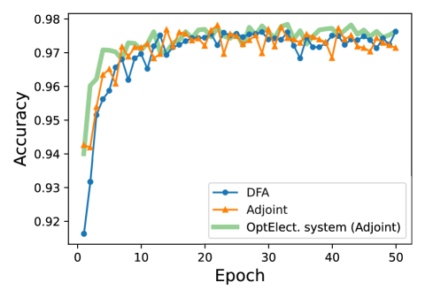
Figure S3: Classification accuracy for the MNIST handwritten digit dataset. Blue circles: DFA–adjoint method, orange triangles: adjoint method applied to additive control model [Eq. (S63)]. Green line: the adjoint method applied to Eq. (5) in the main text. $\alpha$ = 1.

S-VII Numerical simulation

The model equation of the optoelectronic delay system utilized for the numerical simulations in this study is represented as Eq. (5) in the main text. The original model equation proposed by Murphy et al. is given as follows:

$$\frac{\text{d}r_{1}}{\text{d}t} =-\left(\frac{1}{\tau_{L}}+\frac{1}{\tau_{H}}\right)r_{1}(t)-r_{2}(t)+\frac{\beta}{\tau_{L}}\cos^{2}\left[r_{1}(t-\tau_{D})+\phi_{0}\right],$$ (S64)

$$\frac{\text{d}r_{2}}{\text{d}t} =\frac{1}{\tau_{H}}r_{1}(t).$$ (S65)

To apply the system for the present training scheme, two control signals $u_{1}(t)$ and $u_{2}(t)$ were introduced to impact $r_{1}(t-\tau_{D})$ and $\phi_{0}$, respectively, as follows:

$$\frac{\text{d}r_{1}}{\text{d}t} =-\left(\frac{1}{\tau_{L}}+\frac{1}{\tau_{H}}\right)r_{1}(t)-r_{2}(t)+\frac{\beta}{\tau_{L}}\cos^{2}\left[u_{1}(t)r_{1}(t-\tau_{D})+u_{2}(t)\right],$$ (S66)

$$\frac{\text{d}r_{2}}{\text{d}t} =\frac{1}{\tau_{H}}r_{1}(t).$$ (S67)

Additionally, a noise term, $\sigma\xi(t)$, was incorporated into the system to explore noise robustness, where $\sigma$ and $\xi(t)$ represent the noise strength and Gaussian noise with zero mean and unity standard deviation, respectively. The modified system is now represented as follows:

$$\tau_{L}\frac{\text{d}r_{1}}{\text{d}t} =-\left(1+\dfrac{\tau_{L}}{\tau_{H}}\right)r_{1}-\dfrac{1}{\tau_{H}}\int r_{1}dt+\beta\cos^{2}\left[u_{1}(t)r_{1}(t-\tau_{D})+u_{2}(t)\right]+\tau_{L}\sigma\xi(t).$$ (6)

In the main text, $r_{1}(t)$ is expressed as $r(t)$. The default parameter values were set as follows: $\tau_{D}=0.92$ ms, $\tau_{L}=15.9\ \mu$s, and $\tau_{H}=1.59$ ms, $T_{e}=3\tau_{D}$, and $T_{c}=\tau_{D}$. The initial values of the control signals were $u_{1}(t)=1$ and $u_{2}(t)=-\pi/4$, respectively. These parameter values are similar with the default values used in Ref. [38] in the main text.

For the MNIST handwritten digit and Fashion-MNIST classifications, we employed the time segment $\Delta t\sim 0.29337\ \mu$s. The input images of the dataset with $28\times 28$ pixels were enlarged twice and transformed into the time series using mask pattern ${\bm{m}}(t)$ defined as $r(t)={\bm{m}}^{\mathrm{T}}(t){\bm{x}}$. The elements of ${\bm{m}}(t)$ were initially set randomly. Thus, the sequence starting from the initial state is generally jagged, as shown in Fig. 2(a) in the main text. The timescale did not match the characteristic timescale of the system dynamics. After time evolution, the high-frequency components were filtered due to the finite time response. Mask pattern ${\bm{m}}(t)$ can be optimized using either the adjoint method or the DFA–adjoint method. For the CIFAR-10, time region for the input signal was divided into $3\times 32^{2}=3072$ segments using $\Delta t\sim 0.74870\ \mu$s. The input images in CIFAR-10, comprising $32\times 32$ RGB pixels, were transformed into the time series as $r(t)={\bm{m}}^{\mathrm{T}}(t){\bm{x}}$.

Loss function $L$ and $\mbox{\boldmath$G$}_{\mathrm{out}}$ were set as the cross entropy and softmax functions for the present classification problems, respectively. To optimize variables ${\bm{u}}(t)$, ${\bm{m}}(t)$, and ${\bm{w}}(t)$, we utilized the Adam optimizer with the recommended hyperparameters, although $\alpha=10^{-4}$ was employed to optimize ${\bm{m}}(t)$. For the training, the minibatch with a size of $100$ was utilized.

Table S2 shows the means and the standard variations of the classification accuracy computed by five simulations with different pseudo-random numbers for each method. In Fig. 2(b) in the main text, we show a typical learning curve obtained by a single simulation and the averaged learning curve obtained by five simulations as the black solid line with circles and blue solid line, respectively. To evaluate the mean accuracy depicted in Figs. 3(b), 3(c), and 3(d), we used the accuracy at the last five epochs for a mean value.

The simulation code for this study was written on Python with NumPy, an ordinary library of Python. The training time in the DFA–adjoint method was measured as the time required for the product operation described in Eq. (3) [or Eq. (S50)] and the update of ${\bm{u}}(t)$ described in Eq. (S51). As the training time in the adjoint method, the time required to compute the (reverse) time evolution of ${\bm{p}}(t)$ following Eq. (2) [or Eq. (S45)] and the update ${\bm{u}}(t)$ described in Eq. (S47) was measured. We measured the mean training time over 20 runs, employing time() function of time library of Python, where the relative standard deviations of the values were approximately less than 5 % with the exception of 11.1 % in the adjoint method with $\tau_{D}=0.92$ ms. Because the actual computational time depends on implementation details, numerical libraries, and programming language used, we should focus on the relative difference of the time in this study.

Table S2: Mean classification accuracy (standard deviation) obtained by five runs for MNIST, Fashion-MNIST, and CIFAR-10 datasets.

Methods	MNIST	Fashion-MNIST	CIFAR-10
DFA–adjoint	0.973 (0.00075)	$0.866(0.0074)$	0.466 (0.0086)
Adjoint control	0.977 (0.0014)	$0.881(0.0012)$	0.507 (0.0075)
ELM (w/o control)	0.869 (0.0055)	$0.792(0.0055)$	0.275 (0.0012)

In the numerical simulations, we used different parameter values from those used in the experiment. Even when the experimental parameter values ($\tau_{D}$ = 1.022 $\mu$s, $\tau_{L}$ = 1.59 ns, and $\tau_{H}$ = 530 ns) were applied in the numerical simulations, a similar classification accuracy was achieved. The results are shown in Fig. S4. The accuracy was similar with that shown in Fig. 2(b) of the main text.

In the numerical results reported in the main text, $N_{\mathrm{layers}}=T_{e}/\tau_{D}$ was fixed as $3$. $N_{\mathrm{layers}}$ corresponds to the effective number of layers. We evaluated how classification accuracy depends on $N_{\mathrm{layers}}$ for a simple nonlinear two-class classification task for systematic investigations while saving computational time. The result is shown in Fig. S5, where the classification accuracy is mapped on $(\beta,N_{\mathrm{layers}})$ plane. As observed in this figure, the classification accuracy approaches 1 for $N_{\mathrm{layers}}\geq 2$ and $\beta\geq 2$. In particular, for $2\leq N_{\mathrm{layers}}\leq 4$, high accuracy was obtained for a wide range of $\beta$ in this task. For a large $\beta$-values, the delay system used in this study exhibited chaotic behavior; the high sensitivity to initial states led to the instability of classification, particularly, for a long $N_{\mathrm{layers}}$. Consequently, the classification accuracy decreased.

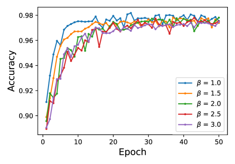
Figure S4: Numerical results of classification accuracy. The parameter values used in the numerical simulations were set as the same values as those used in the experiment.

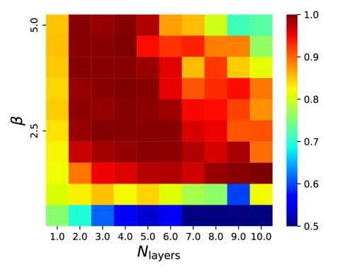
Figure S5: Classification accuracy on $(\beta,N_{\mathrm{layers}})$ plane.

S-VIII Measurement in alignment effect

As discussed in the main text, the update vector $\delta{\bm{u}}_{DFA}$ in the DFA–adjoint method tends to align with the update vector $\delta{\bm{u}}_{adj}$ in the adjoint method. To evaluate the alignment effect, we measured the cosine similarity $C$ between $\delta{\bm{u}}_{DFA}$ and $\delta{\bm{u}}_{adj}$, which is defined as follows:

$$C=\dfrac{\langle\delta{\bm{u}}_{DFA}^{\mathrm{T}}\delta{\bm{u}}_{adj}\rangle_{t}}{\lVert\delta{\bm{u}}_{DFA}\rVert_{2}\lVert\delta{\bm{u}}_{adj}\rVert_{2}},$$ (S68)

where $\langle\cdot\rangle_{t}$ and $\lVert\cdot\rVert$ represent the time average and $L_{2}$ vector norm, respectively. The update vector $\delta{\bm{u}}_{adj}$ was computed based on the trained states by the DFA–adjoint method. In Fig. 2(c) of the main text, we depict the mean and standard deviation of the cosine similarity at each epoch.

S-IX Experiment

The time evolution of the optoelectronic delay system used in this experiment is governed by the following equation:

$$\tau_{L}\frac{\text{d}r}{\text{d}t} =-\left(1+\dfrac{\tau_{L}}{\tau_{H}}\right)r-\dfrac{1}{\tau_{H}}\int rdt$$

$$+\beta\cos^{2}\left(u(t)+\phi_{in}\right)\cos^{2}\left(r(t-\tau_{D})+\phi_{fb}\right)+\sigma\xi(t),$$ (S69)

where $r(t)$ denotes the light intensity (system variable). $\tau$, $\beta$, $\tau_{L}$, and $\tau_{H}$ in the equation denote the feedback delay time, normalized gain coefficient, and time constants of the low- and high-pass filters, respectively. Specific parameter values were chosen as follows: $\tau_{D}=1.022$ $\mu$s, $\tau_{L}=1.59$ ns, and $\tau_{H}=530$ ns. The bias points of MZM1 and MZM2 were set as $\phi_{in}=-\pi/4$ and $\phi_{fb}=-\pi/4$, respectively. In the experimental setup shown in Fig. 4(a), encoding the input ${\bm{x}}$ as the initial state of $r(t)$ for $-\tau_{D}\leq t\leq 0$ proved challenging. Instead, we set the input data as the control signal $u(t)={\bm{m}}^{\mathrm{T}}(t){\bm{x}}$ for $-\tau_{D}\leq t<0$. The softmax function was used in the output layer and computed on a digital computer in this experiment, although an efficient hardware implementation can be achieved using a field programmable gate array or an application-specific integrated circuit. The DFA–adjoint method was employed to train the control signal $u(t)$ for $t>0$ and mask pattern ${\bm{m}}(t)$ for $-\tau_{D}\leq t\leq 0$.

For training, we randomly selected the 3000 images for the training set and 500 images for the test set from the original MNIST dataset. The distribution of the sampled images across digit labels is summarized in Table S3. For the test dataset, the confusion matrix is shown in Fig. S6.

Table S3: Number of the MNIST image samples used for training and testing.

Label	0	1	2	3	4	5	6	7	8	9
Training	285	339	299	295	325	273	306	329	261	288
Test	42	67	55	45	55	50	43	49	40	54

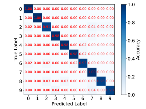
Figure S6: Confusion matrix. 500 test images randomly sampled from the original MNIST dataset was used for the experiment.