Algorithmic approaches to avoiding bad local minima in nonconvex inconsistent feasibility

Abstract

The main challenge of nonconvex optimization is to find a global optimum, or at least to avoid “bad” local minima and meaningless stationary points. We study here the extent to which algorithms, as opposed to optimization models and regularization, can be tuned to accomplish this goal. The model we consider is a nonconvex, inconsistent feasibility problem with many local minima, where these are points at which the gaps between the sets are smallest on neighborhoods of these points. The algorithms that we compare are all projection-based algorithms, specifically cyclic projections, the cyclic relaxed Douglas-Rachford algorithm, and relaxed Douglas-Rachford splitting on the product space. The local convergence and fixed points of these algorithms have already been characterized in pervious theoretical studies. We demonstrate the theory for these algorithms in the context of orbital tomographic imaging from angle-resolved photon emission spectroscopy (ARPES) measurements, both synthetically generated and experimental. Our results show that, while the cyclic projections and cyclic relaxed Douglas-Rachford algorithms generally converge the fastest, the method of relaxed Douglas-Rachford splitting on the product space does move away from bad local minima of the other two algorithms, settling eventually on clusters of local minima corresponding to globally optimal critical points.

Keywords: nonconvex optimization, projection algorithm, Douglas-Rachford splitting, inconsistent feasibility, phase retrieval

Mathematics Subject Classification: 65K10, 65K05, 90C26, 49M27, 49J53, 49K40, 49M05

1 Introduction

The Douglas-Rachford algorithm is frequently used in the optics community as an alternative to cyclic projections in order to avoid undesirable local minima. There is good reason for this: the Douglas-Rachford mapping does not have fixed points when applied to inconsistent feasibility problems [14], so it cannot get stuck in bad local minima. This advantage comes at the cost of not converging at all. The standard practice in the optics community is to run a few iterations of a Douglas-Rachford-type algorithm, and then to run several iterations of cyclic projections to arrive at a satisfactory fixed point [15]. We show in this paper that this practice, while not unreasonable, has things the wrong way around: one should start with cyclic projections and then run a relaxed Douglas-Rachford algorithm in order to move out of undesirable local domains of attraction.

Relaxations of the Douglas-Rachford algorithm have been extensively studied primarily with the goal of stabilizing the original Douglas-Rachford mapping [14, 11, 21, 5, 24] but also with an eye toward obtaining/preserving linear convergence for nonconvex feasibility [12, 13, 6, 17]. Beyond not converging for inconsistent feasibility problems, another drawback of the Douglas-Rachford algorithm is that there is not a unique way to extend it to splitting with more than two operators. For multi-set feasibility, one possibility is to formulate the problem as two-set feasibility between the sets on the product space and the diagonal of the product space [22]. Another approach, first studied in [5], is to apply the two-operator Douglas-Rachford mappings pairwise in a cyclic manner. Obviously these two different approaches lead to different algorithms with different convergence properties. A cyclic version of the relaxed Douglas-Rachford mapping studied in [14] was first proposed in the convex setting in [18], and more recently the nonconvex setting is developed in [8], where the fixed points are characterized and local convergence of the algorithm is established under the weakest assumptions to date.

In this work we present numerical results showing the relative merits of all of the above strategies, leading to the observation that the relaxed Douglas-Rachford algorithm is a reasonable candidate for avoiding bad fixed points of the cyclic projections algorithm. While this observation was not unexpected, based on the known characterization of the fixed points, it was surprising to see that the product-space, relaxed Douglas-Rachford algorithm could be used to “clean up” the bad cyclic projections fixed points. Our numerical demonstration focuses on the problem of tomographic reconstruction of molecular electronic structures from angle-resolved photoemission spectroscopy (ARPES) data studied in [9]. We refer to this as the photoemission orbital tomography problem. While this problem is quite specific, it has features that are common in many applications, and therefore serves as a good test case. All of these algorithms have been compared on a number of different related problem classes [19], but our results for the orbital tomography problem provide a more complete picture than the conclusions resulting from [19]. In particular, our results show that the cyclic relaxed Douglas-Rachford algorithm which appeared to be the best performer in most of the tests in [19], is not a good candidate for many-set feasibility problems like the orbital tomography problem.

In Section 2, we recall the mathematical definitions necessary for the convergence statements in this study. In Section 3, we review the physical ARPES orbital tomography problem and reformulate this as a feasibility problem, outline the numerical methods used for its solution (Section 3.2). Since all of the algorithms in this comparison are built from projection operators, we derive the formulas for the projectors onto the sets in the ARPES orbital tomography problem in Section 3.3, and verify the main assumption for local linear convergence of the three algorithms for the ARPES orbital tomography problem, with explicit formulations of the parameters involved in the rate constant (Section 3.4). In Section 4, we present numerical results using the dataset from [9]. Compared to the current state-of-the-art cyclic projection method, CDR$\lambda$ achieves a higher success rate. Additionally, DR$\lambda$ demonstrates superior performance in avoiding bad local minima. The code and data for the laboratory data is available from [3].

2 Preliminaries

Throughout this paper, $\mathbb{E}$ is a finite-dimensional Euclidean space. In particular, set $\mathbb{E}=\mathbb{C}^{N}$. We recall definitions of almost nonexpansive/almost $\alpha$-firmly nonexpensive (see [4, Definition 1]). Let $D$ be a nonempty subset of $\mathbb{E}$ and let $T$ be a (set-valued) mapping from $D$ to $\mathbb{E}$, i.e., $T:D\rightrightarrows\mathbb{E}$.

1. $T$ is said to be pointwise almost nonexpansive on $D$ at $y\in D$ if there exists a constant $\epsilon\in[0,1)$ such that

   $$\|x^{+}-y^{+}\|\leq\sqrt{1+\epsilon}\|x-y\|\,,$$ (1)

   $$~\forall~y^{+}\in Ty\mbox{ and }\forall~x^{+}\in Tx\mbox{ whenever }x\in D.$$

2. $T$ is pointwise almost $\alpha$-firmly nonexpensive (abbreviated pointwise a$\alpha$-fne) at $y\in D$ whenever there exists $\alpha\in(0,1)$ and $\epsilon\in[0,1)$:

   $$\forall x\in D\,,\,\forall x^{+}\in Tx\,,\,\forall y^{+}\in Ty\,,$$ (2)

   $$\|x^{+}-y^{+}\|^{2}\leq(1+\epsilon)\|x-y\|^{2}-\frac{1-\alpha}{\alpha}\psi(x,y,x^{+},y^{+})\,,$$ (3)

   where

   $$\psi(x,y,x^{+},y^{+}):=\|(x^{+}-x)-(y^{+}-y)\|^{2}$$ (4)

   denotes transport discrepency. When $\epsilon=0$, $T$ is said to be pointwise nonexpansive on $D$ at $y\in D$ (abbreviated pointwise $\alpha$-fne)

The projector of a point $x$ onto the set $A\subset\mathbb{E}$, is the mapping of $x$ to the set of points where the distance to the set $A$ is attained,

$$P_{A}x:=\operatorname{argmin}_{a\in A}\|a-x\|.$$

When $A$ is closed and non-empty this set is nonempty. If $y\in P_{A}x$, then $y$ is called a projection of $x$ on $A$. The reflector is defined by $R_{C}:=2P_{C}-\mathrm{Id}$. If $y\in R_{C}x$, then $y$ is called reflection of $x$ across $C$.

We say that a closed set $A$ is prox-regular at $\bar{x}\in A$ if the projector $P_{A}$ is single-valued near $\bar{x}$, as stated in [23, Theorem 1.3]. Any closed convex set, for example, is prox-regular at any point in that set since the projector is everywhere single-valued.

Given set-value mapping $T:\mathbb{E}\rightrightarrows\mathbb{E}$. Inverse operator $T^{-1}$ is defined by $T^{-1}(a):=\{x\in\mathbb{E}\ |\ a\in Tx\}$ and the graph of the mapping $T$ is the set $\mathrm{gph}(T):=\{(x,y):x\in\mathbb{E}\,,\,y\in Tx\}$ which is a subset of $\mathbb{E}\times\mathbb{E}$.

A proximal normal cone of a set $\Omega\subset\mathbb{E}$ at $\bar{a}\in\Omega$ is defined by

$$N^{P}_{\Omega}(\bar{a}):=\text{cone}\left(P^{-1}_{\Omega}\bar{a}-\bar{a}\right).$$

The limiting (proximal) normal cone of $C$ at $\bar{a}$ is defined by

$$N_{\Omega}(\bar{a}):=\limsup\limits_{x\to\bar{a}}N_{\Omega}^{P}(x),$$

where the limit superior is taken in the sense of Painlevé–Kuratowski outer limit. When $\bar{a}\not\in\Omega$, all normal cones at $\bar{a}$ are empty (by definition). A set $\Omega\subset\mathbb{E}$ is called $\epsilon$-super-regular at a distance relative to $\Lambda\subset\mathbb{E}$ at $\bar{x}$ with constant $\epsilon$ whenever

$$\exists~U_{\epsilon}\subset\mathbb{E}~\mbox{ open}~:~ \bar{x}\in U_{\epsilon},\mbox{ and }$$

$$\langle{v-(y^{\prime}-y),y-x\rangle}\leq\epsilon_{U}\|v-(y^{\prime}-y)\|\|y-x\|$$

$$\forall y^{\prime}\in U_{\epsilon}\cap\Lambda,\quad\forall y\in P_{\Omega}(y^{\prime}),$$

$$\forall(x,v)\in\left\{(x,v)\in\mathrm{gph}N^{\text{\rm prox}}_{\Omega}~\mid~x+v\in U_{\epsilon},~x\in P_{\Omega}(x+v)\right\}.$$

The set $\Omega$ is called super-regular at a distance relative to $\Lambda$ at $\bar{x}$ if it is $\epsilon$-super-regular at a distance relative to $\Lambda$ at $\bar{x}$ for all $\epsilon>0$.

By [20, Proposition 3.1] we have the following implications:

$$\begin{array}[]{ccc}\text{convexity}&\Rightarrow\text{prox-regularity}&\Rightarrow\epsilon\text{-super-regularity at a distance}.\end{array}$$

For a subset $A\subset\mathbb{E}$, the image of $A$ under $T$, denoted by $TA$, is defined by

$$TA:=\bigcup_{a\in A}Ta\,.$$

When the mapping $T:\mathbb{E}\rightrightarrows\mathbb{E}$ is single-valued at $y\in\mathbb{E}$, that is if $Ty=\{z\}$ is a singleton,then we simply write $z=Ty$. The mapping $T$ is single-valued on $U\subset E$ if it is single-valued at all points $y\in U$. With $T,Q:\mathbb{E}\rightrightarrows\mathbb{E}$ being set-value mappings, the composite $TQ$ or $T\circ Q$ from $\mathbb{E}$ to $\mathbb{E}$ is defined by

$$TQx=(T\circ Q)x:=\bigcup_{y\in Qx}Ty.$$ (6)

The set of fixed points of $T$ is defined by $\mathrm{Fix}\ T:=\{x\in\mathbb{E}\,|\,x\in Tx\}.$

3 The 3D Photoemission orbital tomography problem

3.1 Problem statement

We now specialize the theory in [8] to the very concrete problem of orbital tomography with angle-resolved photoemission spectroscopy (ARPES) data. The physical domain of the objects which are to be recovered from ARPES data is represented by $D\subset\mathbb{R}^{3}$. A point in $D$ corresponding to an index $(i,j,l)$ is denoted $(x_{i},y_{j},z_{l})$, where $(i,j,l)\in\mathbb{I}:=\{1,\dots,N_{x}\}\times\{1,\dots,N_{y}\}\times\{1,\dots,N_{z}\}$. Here, $N_{*}$ represents the number of voxels in the $x$, $y$, and $z$ directions, respectively. The total number of voxels $|\mathbb{I}|$ is denoted by $N=N_{x}\times N_{y}\times N_{z}$. The “object” in question is the spatial representation of a molecular orbital, modeled for convenience as a complex-valued vector $u\in\mathbb{C}^{N}$, each element of which, $u_{(i,j,l)}$, representing the “value” (yielding the probability density by Born’s rule) of the electronic orbital at the points $(x_{i},y_{j},z_{l})\in D$. The only complex values that the orbital $u_{(i,j,l)}$ takes are either $u_{(i,j,l)}=+|u_{(i,j,l)}|$ or $u_{(i,j,l)}=-|u_{(i,j,l)}|$ corresponding to the charge.

The data domain (image space of the model), where the ARPES data is observed, is denoted by ${\widehat{D}}\subset\mathbb{R}^{3}$. This is discretized in a similar manner to the discretization of the domain, but potentially with different numbers of pixels/voxels. The point in ${\widehat{D}}$ corresponding to the index $(i,j,l)\in{\widehat{\mathbb{I}}}:=\{1,\dots,{\widehat{N}}_{x}\}\times\{1,\dots,{\widehat{N}}_{y}\}\times\{1,\dots,{\widehat{N}}_{z}\}$ is denoted $({\widehat{x}}_{i},{\widehat{y}}_{j},{\widehat{z}}_{l})$. Here, ${\widehat{N}}_{*}$ represents the number of voxels in the ${\widehat{x}}$, ${\widehat{y}}$, and ${\widehat{z}}$ directions in the image space. The total number of voxels $|{\widehat{\mathbb{I}}}|$ is denoted by ${\widehat{N}}={\widehat{N}}_{x}\times{\widehat{N}}_{y}\times{\widehat{N}}_{z}$.

The mathematical model for 3D photoemission orbital tomography is described in detail in [9]. Since our primary interest is the mathematical structure of the problem, we will not derive the mathematical model for the data. In principle, the image ${\widehat{u}}$ of the object $u$ to be recovered, is also a complex-valued vector ${\widehat{u}}\in\mathbb{C}^{\widehat{N}}$, each element of which, ${\widehat{u}}_{(i,j,l)}$, representing the “value” of the electronic orbital upon transformation to the image domain at the points $({\widehat{x}}_{i},{\widehat{y}}_{j},{\widehat{z}}_{l})\in{\widehat{D}}$. The model for the mapping to the image domain is simply a Fourier transform of the electronic orbitals, that is $\mathcal{F}u={\widehat{u}}$ where $\mathcal{F}~:~\mathbb{C}^{N}\to\mathbb{C}^{\widehat{N}}$ denotes the discrete Fourier transform.

The physical measurements are the element-wise amplitudes of ${\widehat{u}}$ on discrete spheres in ${\widehat{D}}$. In other words, the data, denoted $b_{(i,j,l)}\in\mathbb{R}_{+}$, specifies the amplitudes $|{\widehat{u}}_{(i,j,l)}|$ only for indexes $(i,j,l)\in\mathbb{S}\subset{\widehat{\mathbb{I}}}$. The set of all possible vectors $u$ satisfying the data measurements is defined by

$$\text{M}:=\{u\in{{\mathbb{C}}^{N}}\mid\ |{\widehat{u}}_{(i,j,l)}|=b_{(i,j,l)},\ (i,j,l)\in\mathbb{S}\}\,.$$ (7)

The fact that the indexes $\mathbb{S}$ correspond to several spheres in ${\widehat{D}}$ is of no consequence to our present analysis; for our purposes it is only relevant that $\mathbb{S}$ is a subset of all the indexes ${\widehat{\mathbb{I}}}$. In [9] the authors find that four measurements are enough for reasonable reconstructions. However, the challenge lies in the significant number of local solutions that appear in the reconstructions. The numerical results reported in Section 4 show that the CDR$\lambda$ algorithm can produce fewer bad local reconstructions than the cyclic projections algorithm used in [9].

We will use the same feasibility model as in [9]. To recall, we formulate orbital tomography reconstruction problem as a multi-set feasibility model:

$$\text{Find}\ u\in\text{SYM}\cap\text{SR}\cap\text{SUPP}\cap\text{LF}\cap\text{M},$$ (8)

where

• M is the measurement constraint set defined in (7).

• LF is the set of points in the object domain that satisfy a support constraint in the image domain:

  $$\text{LF}:=\{u\in{{\mathbb{C}}^{N}}\mid\ |{\widehat{u}}_{(i,j,l)}|=0,\ ({\widehat{x}}_{i},{\widehat{y}}_{j},{\widehat{z}}_{l})\notin B_{\overline{r}}\}\,.$$ (9)

  where $B_{\overline{r}}$ is a ball in ${\widehat{D}}$.

• SUPP is the set of points that satisfy a support constraint in the object domain:

  $$\text{SUPP}=\{u\in\mathbb{C}^{N}\mid\ u\Omega=u\}$$ (10)

  for some symmetric binary mask $\Omega\in\{0,1\}^{N}$.

• SR is the set of points that satisfy a sparse real constraint:

  $$\text{SR}:=\{u\in{{\mathbb{C}}^{N}}\mid\ \|u\|_{0}\leq s\mbox{ and }\text{Im}(u)=0\},$$ (11)

  where, $s>0$ is given, Im$(u)$ is the imaginary part of the complex vector $u$, and $\|\cdot\|_{0}$ denotes the counting function that counts all non-zero elements.

• SYM is the symmetry and anti-symmetry constraint set:

  $$\text{SYM}:=\left\{u\in{\mathbb{C}^{N}}\mid u_{(i,j,l)}=u_{(N_{x}-i+1,j,l)}=-u_{(i,N_{y}-j+1,l)}=-u_{(i,j,N_{z}-l+1)}\,,\,(i,j,l)\in\mathbb{I}\right\}.$$ (12)

The sets M and SR are nonconvex, so, without additional assumptions, convergence to a solution of (8) can only be guaranteed locally. Note, however, that the sets SUPP and LF, though convex, do not in general have points in common: any vector in SUPP that is not periodic will not belong to LF. The feasibility model (8) is therefore inconsistent and there do not exist solutions to (8). We therefore must be content with finding points that come as close as possible to satisfying all of the constraints.

3.2 Projection methods

We compare the performance of three different algorithms, all of which can be written as the following general fixed point iteration.

Algorithm 1 General fixed point iteration

 Initialization: Set $\text{tol}>0$, $n=0$, $\text{monitor}^{(0)}>\text{tol}$, $u^{(0)}\in\mathbb{C}^{N}$.

 while $\text{monitor}^{(n)}>\text{tol}$ do

  Set $n=n+1$. Compute

$$u^{(n)}\in Tu^{(n-1)}$$ (13)

and update $\text{monitor}^{(n)}$.

 end while

The three algorithms represent different instantiations of the mapping $T$, namely cyclic projections, $T^{\text{CP}}_{\text{orbit3D}}$, cyclic relaxed Douglas-Rachford $T^{\text{CDR}\lambda}_{\text{orbit3D}}$ and relaxed Douglas-Rachford on the product space, $T^{\textbf{DR}\lambda}_{\text{orbit3D}}$. Note that the exit criterion is based on the difference in the shadows of the iterates $u^{(n)}$ onto the set SYM, i.e.,

$$\text{monitor}^{(n)}:=\text{monitor}^{(n)}_{1}:=|P_{\text{SYM}}u^{(n)}-P_{\text{SYM}}u^{(n-1)}|.$$ (14)

For the cyclic projection mapping $T^{\text{CP}}_{\text{orbit3D}}$, the shadows are just the iterates themselves. For the relaxed Douglas-Rachford algorithm below, this will not be the case.

We recall the cyclic projection algorithm in [9] to numerically solve problem (8). Define

$$T^{{\text{CP}}}_{\text{orbit3D}}:=P_{\text{SYM}}\circ P_{\text{SR}}\circ P_{\text{SUPP}}\circ P_{\text{LF}}\circ P_{\text{M}}.$$ (15)

In what follows $T^{\mathrm{DR}\lambda}_{A,B}$ denotes the relaxed Douglas-Rachford operator with respect to the sets $A,B$ for a fixed relaxation parameter $\lambda\in[0.1]$, i.e.,

$$T^{\mathrm{DR}\lambda}_{A,B}=\frac{\lambda}{2}(R_{A}R_{B}+\mathrm{Id})+(1-\lambda)P_{B}.$$ (16)

This method has been studied in [18] where quantitative convergence guarantees and characterization of the fixed points set were established. When there are more than two sets, as here, there are a number of different options for applying relaxed Douglas-Rachford-type splitting. Two options that we compare here are cyclic relaxed Douglas-Rachford and relaxed Douglas-Rachford on the product space. The cyclic version takes the form

$$T^{\text{CDR$\lambda$}}_{\text{orbit3D}}:=T^{\mathrm{DR}\lambda}_{\text{SYM},\text{SR}}\circ T^{\mathrm{DR}\lambda}_{\text{SR},\text{SUPP}}\circ T^{\mathrm{DR}\lambda}_{\text{SUPP},\text{LF}}\circ T^{\mathrm{DR}\lambda}_{\text{LF},\text{M}}\circ T^{\mathrm{DR}\lambda}_{\text{M},\text{SYM}}.$$ (17)

To derive the product space formulation, let $\mathbf{u}=(u_{1},u_{2},u_{3},u_{4},u_{5})$, $C=\text{SYM}\times\text{SR}\times\text{SUPP}\times\text{LF}\times\text{M}$ and denote by $D$ the diagonal set of $\mathbb{C}^{N^{5}}$, which is defined by $\{\mathbf{u}=(u,u,u,u,u)\in\mathbb{C}^{N^{5}}\}$. The operator $T^{\text{DR$\lambda$}}_{\text{orbit3D}}$ is given by

$$T^{\textbf{DR$\lambda$}}_{\text{orbit3D}}:=\frac{\lambda}{2}(R_{D}R_{C}+\mathrm{Id})+(1-\lambda)P_{C},$$ (18)

where

$$P_{C}\mathbf{u}=(P_{\text{SYM}}u_{1},P_{\text{SR}}u_{2},P_{\text{SUPP}}u_{3},P_{\text{LF}}u_{4},P_{\text{M}}u_{5}),$$ (19)

and

$$[P_{D}\mathbf{u}]_{i}=\frac{P_{\text{SYM}}u_{1}+P_{\text{SR}}u_{2}+P_{\text{SUPP}}u_{3}+P_{\text{LF}}u_{4}+P_{\text{M}}u_{5}}{5},\,\forall i=1,2,3,4,5.$$ (20)

The volume of the solutions to the problem is quintupled, but the computation of projections can be done in parallel. In the consistent case, this algorithm would be used to solve the problem

$$\text{Find }\mathbf{u}\in C\cap D.$$ (21)

In this case, it is easy to see that each entry of the solution $\mathbf{u}$ is a point in $\text{SYM}\cap\text{SR}\cap\text{SUPP}\cap\text{LF}\cap\text{M}$. In the inconsistent case, the fixed points of (18) are given abstractly by [17, Theorem 3.13] where the characterization is in the product space. The fixed points of $T^{\text{CDR$\lambda$}}_{\text{orbit3D}}$ were characterized in [8, Theorem 3.2].

To evaluate the quality of (approximate) fixed points, we calculate the gap. The gap at a point is defined as the sum of the distances between the sets at that point. An (approximate) fixed point that achieves a smaller gap is considered better. Let $u^{(n)}$ be the $n$-th iterate of algorithm 1. Set

$$\check{u}^{(n)}=\begin{cases}u^{(n)}&{\text{ if }T=T^{\text{CP}}_{\text{orbit3D}}}\\ P_{\text{SYM}}u^{(n)}&{\text{ if }T=T^{\text{CDR$\lambda$}}_{\text{orbit3D}}}\\ P_{\text{SYM}}u_{1}^{(n)}&\text{ if $T=T^{\textbf{DR}\lambda}_{\text{orbit3D}}$.}\end{cases}$$ (22)

The gap at $n$-th iteration is computed as follows:

$$\text{gap}^{(n)}:=\text{gap}^{(n)}(\check{u}^{(n)}):=\frac{\text{gap}^{(n)}_{\text{SYM}-\text{M}}+\text{gap}^{(n)}_{M-\text{LF}}+\text{gap}^{(n)}_{\text{LF}-\text{SUPP}}+\text{gap}^{(n)}_{\text{SUPP}-\text{SR}}+\text{gap}^{(n)}_{\text{SR}-\text{SYM}}}{\|b\|},$$

where

$$\begin{array}[]{rcl}&\text{gap}^{(n)}_{\text{SYM}-\text{M}}&:=\|\check{u}^{(n)}-P_{\text{M}}\check{u}^{(n)}\|,\\ &\text{gap}^{(n)}_{M-\text{LF}}&:=\|P_{\text{M}}\check{u}^{(n)}-P_{\text{LF}}P_{\text{M}}\check{u}^{(n)}\|\,,\\ &\text{gap}^{(n)}_{\text{LF}-\text{SUPP}}&:=\|P_{\text{LF}}P_{\text{M}}\check{u}^{(n)}-P_{\text{SUPP}}P_{\text{LF}}P_{\text{M}}\check{u}^{(n)}\|\,,\\ &\text{gap}^{(n)}_{\text{SUPP}-\text{SR}}&:=\|P_{\text{SUPP}}P_{\text{LF}}P_{\text{M}}\check{u}^{(n)}-P_{\text{SR}}P_{\text{SUPP}}P_{\text{LF}}P_{\text{M}}\check{u}^{(n)}\|\,,\\ &\text{gap}^{(n)}_{\text{SR}-\text{SYM}}&:=\|P_{\text{SR}}P_{\text{SUPP}}P_{\text{LF}}P_{\text{M}}\check{u}^{(n)}-P_{\text{SYM}}P_{\text{SR}}P_{\text{SUPP}}P_{\text{LF}}P_{\text{M}}\check{u}^{(n)}\|.\end{array}$$

For the relaxed Douglas-Rachford operator, we also suggest using the gap for monitoring, i.e. we use the monitor as in (14) and the different gap defined by

$$\text{monitor}^{(n)}:=\text{monitor}^{(n)}_{2}:=|\text{gap}^{(n)}-\text{gap}^{(n-1)}|.$$ (23)

The projection formulas onto the sets will be computed explicitly in the next section.

For simulated data, the error between the iterate $u^{(n)}$ and the ground truth is given by

$$E^{(n)}=\frac{1}{2}\min\left\{\left\|\frac{u^{*}}{\|u^{*}\|}\pm\frac{u^{(n)}}{\|u^{(n)}\|}\right\|\right\}$$ (24)

where $u^{(n)}$ denotes the preferred shadow of the reconstructed orbital at the $n$-the iteration and $u^{*}$ is the ground truth. The error is the minimum of either the sum or the difference of the reconstruction and the reference “truth” to account for the unavoidable global phase ambiguity.

3.3 Projection formulas

We now present the explicit formulations for the projectors onto the sets in (8). A projection of $u$ onto the set M with infinite precision arithmetic is computed by [16, Theorem 4.2]

$$P_{\text{M}}u:=\left\{\mathcal{F}^{-1}v~|~v_{(i,j,l)}\in\begin{cases}\left\{b_{(i,j,l)}\frac{{\widehat{u}}_{(i,j,l)}}{|{\widehat{u}}_{(i,j,l)}|}\right\}&\mbox{ if }|{\widehat{u}}_{(i,j,l)}|\neq 0\\ \left\{b_{(i,j,l)}e^{\mathbf{i}\theta}\mid\theta\in[0,2\pi]\mbox{ and $\mathbf{i}^{2}=-1$}\right\}&\mbox{ else}\end{cases}\right\}$$ (25)

where $\mathcal{F}^{-1}$ is the discrete inverse Fourier transform. Note that $P_{\text{M}}u$ is in general a set; any element from this set will do. This formula, since it involves division by a possibly small number, is not recommended numerically [16, Corollary 4.3]. Since our primary interest here is the convergence theory under the assumption of exact arithmetic, we will ignore this important detail and just caution readers against using this formula in practice.

The projector $P_{\text{LF}}$ is given by

$$P_{\text{LF}}u:=\mathcal{F}^{-1}(v),\quad\mbox{ where }\quad v_{(i,j,l)}=\begin{cases}{\widehat{u}}_{(i,j,l)}&\text{ if $({\widehat{x}}_{i},{\widehat{y}}_{j},{\widehat{z}}_{l})\in B_{\overline{r}}$}\\ 0&\text{otherwise.}\end{cases}$$ (26)

The projector $P_{\text{SUPP}}$ is similar, and can be computed simply by applying the binary mask $\Omega$. More precisely, the projection $u^{\text{SUPP}}$ of a point $u\in\mathbb{C}^{N}$ onto the set SUPP (i.e., $u^{\text{SUPP}}\in P_{\text{SUPP}}u$) is given by

$$u^{\text{SUPP}}_{(i,j,l)}=\begin{cases}u_{(i,j,l)}&\text{if }\Omega_{(i,j,l)}\neq 0,\\ 0&\text{otherwise.}\end{cases}$$ (27)

Both $P_{\text{LF}}$ and $P_{\text{SUPP}}$ are single-valued mappings since LF and SUPP are convex.

Now for the sparse-real constraint set SR. We present the formulation derived in [1, Proposition 3.6]. Define $\mathcal{J}:=2^{\left\{1,2,\dots,2N\right\}}$ and $\mathcal{J}_{s}:=\{J\in\mathcal{J}~|~J\mbox{ has}$ $s\mbox{ elements}\}$. The sparse set

$$\mathcal{A}_{s}:=\left\{x\in\mathbb{C}^{N}~\middle|~\|x\|_{0}\leq s\right\}$$ (28)

can be written as the union of all subspaces indexed by $J\in\mathcal{J}_{s}$ [1, Equation (27d)],

$$\mathcal{A}_{s}=\bigcup_{J\in\mathcal{J}_{s}}A_{J},$$ (29)

where $A_{J}:=\textup{span}\left\{e_{i}~\middle|~i\in J\right\}$ and $e_{i}$ is the $i-$th standard unit vector in $\mathbb{C}^{N}\approx(\mathbb{R}^{2})^{N}$ where $i\in\{1,2,\dots,2N\}$ with the odd indexes being the real parts and the even indexes being the imaginary parts of the points. For $x\in\mathbb{C}^{N}$ we define the set of $s$ largest coordinates in absolute value

$$C_{s}(x):=\left\{J\in\mathcal{J}_{s}~\middle|~\min_{i\in J}|x_{i}|\geq\max_{i\notin J}|x_{i}|\right\}.$$ (30)

The projection of a point $x\in\mathbb{C}^{N}$ onto the sparsity constraint $\mathcal{A}_{s}$ is then given by

$$P_{\mathcal{A}_{s}}x:=\bigcup_{J\in C_{s}(x)}P_{A_{J}}x$$ (31)

Next, denote the real subspace of $\mathbb{C}^{N}$ by $\mathscr{R}^{N}$. Clearly $(P_{\mathscr{R}^{N}}u)_{j}=(\text{Re}(u_{j}),0)$ for $j=1,2,\dots,N$. Now, putting this together with the real-valued constraint, it can easily be shown that the projector onto the set SR is given by

$$P_{\text{SR}}u=P_{\mathcal{A}_{s}}P_{\mathscr{R}^{N}}u.$$ (32)

Indeed, we have

$$\begin{array}[]{rl}P_{\text{SR}}u=&\operatorname{argmin}_{v\in\mathbb{C}^{N}}\left\{\|v-u\|^{2}~|~\|v\|_{0}\leq s\,,\,\text{Im}(v)=0\right\}\\[5.0pt] =&\operatorname{argmin}_{v\in\mathbb{C}^{N}}\left\{\|\text{Re}(v)-\text{Re}(u)\|^{2}+\|\text{Im}(v)\|^{2}~|~\|v\|_{0}\leq s\,\right\}\\[5.0pt] =&\operatorname{argmin}_{v\in\mathcal{A}_{s}}\left\{\|\text{Re}(v)-\text{Re}(P_{\mathscr{R}^{N}}(u))\|^{2}+\|\text{Im}(v)-\text{Im}(P_{\mathscr{R}^{N}}(u))\|^{2}\right\}\\[5.0pt] =&\operatorname{argmin}_{v\in\mathcal{A}_{s}}\left\{\|v-P_{\mathscr{R}^{N}}(u)\|^{2}\right\}\\[5.0pt] =&P_{\mathcal{A}_{s}}P_{\mathscr{R}^{N}}(u)\,.\end{array}$$

There are two things to note about the formula (32): firstly, this projector is set-valued reflecting the fact that the set $\mathcal{A}_{s}$ (and hence SR) is not convex; secondly, if the order of the operations $P_{\mathcal{A}_{s}}P_{\mathscr{R}^{N}}(\cdot)$ is changed, the resulting operator is not the projection onto the set SR.

Finally, we derive the projector onto the symmetry constraint. Let $\Pi_{\mathrm{sym}_{1}},\Pi_{\mathrm{sym}_{2}},\Pi_{\mathrm{sym}_{1}}:\mathbb{C}^{N_{1}\times N_{2}\times N_{3}}\to\mathbb{C}^{N_{1}\times N_{2}\times N_{3}}$ be linear operators defined by

$$\begin{array}[]{rl}&\Pi_{\mathrm{sym}_{1}}u:=u^{T_{1}}=[u^{T_{1}}_{(i,j,l)}]_{(i,j,l)\in\mathbb{I}}\mbox{ where }u^{T_{1}}_{(i,j,l)}=u_{(N_{1}-i+1,j,l)}\,,\\[5.0pt] &\Pi_{\mathrm{sym}_{2}}u:=u^{T_{2}}=[u^{T_{2}}_{(i,j,l)}]_{(i,j,l)\in\mathbb{I}}\text{ with }u^{T_{2}}_{(i,j,l)}=u_{(i,N_{2}-j+1,l)}\,,\\[5.0pt] &\Pi_{\mathrm{sym}_{3}}u:=u^{T_{3}}=[u^{T_{3}}_{(i,j,l)}]_{(i,j,l)\in\mathbb{I}}\text{ with }u^{T_{3}}_{(i,j,l)}=u_{(i,j,N_{3}-l+1)},\,\,(i,j,l)\in\mathbb{I}.\end{array}$$ (33)

These operators are simply transposition operators in the respective coordinate axes of the tensors.

Lemma 1.

The symmetry set SYM can be expressed as:

$$\text{SYM}=\text{SYM}^{3}_{-}\cap\text{SYM}^{2}_{-}\cap\text{SYM}^{1}_{+},$$ (34)

where

$$\begin{array}[]{rl}&\text{SYM}^{1}_{+}:=\{u\in\mathbb{C}^{N}\mid u_{(i,j,l)}=u_{(N_{1}-i+1,j,l)}\},\\ &\text{SYM}^{2}_{-}:=\{u\in\mathbb{C}^{N}\mid u_{(i,j,l)}=-u_{(i,N_{2}-j+1,l)}\},\\ &\text{SYM}^{3}_{-}:=\{u\in\mathbb{C}^{N}\mid u_{(i,j,l)}=-u_{(i,j,N_{3}-l+1)}\}.\end{array}$$ (35)

Moreover,

$$P_{\text{SYM}}=P_{\text{SYM}^{3}_{-}}\circ P_{\text{SYM}^{2}_{-}}\circ P_{\text{SYM}^{1}_{+}}$$ (36a)

where

$$P_{\text{SYM}^{1}_{+}} = \frac{\mathrm{Id}+\Pi_{\mathrm{sym}_{1}}}{2}$$ (36b)

$$P_{\text{SYM}^{2}_{-}} = \frac{\mathrm{Id}-\Pi_{\mathrm{sym}_{2}}}{2}$$ (36c)

$$P_{\text{SYM}^{2}_{-}} = \frac{\mathrm{Id}-\Pi_{\mathrm{sym}_{3}}}{2}$$ (36d)

Proof.

The representation (34) follows immediately from the definition of the set SYM (12).

It is easy to see that $\text{SYM}^{1}_{+},\text{SYM}^{2}_{-},\text{SYM}^{3}_{-}$ are subspaces of the Hilbert space $\mathbb{C}^{N}$. The formulas for the projections onto these subspaces, (36b)-(36d) follow from [7, Section 9.7, exercise 2]. Now, by [25], from any starting point $u$, the cyclic projections algorithm applied to subspaces converges to the projection of $u$ onto the intersection of the subspaces. A routine calculation shows that $u^{(1)}:=P_{\text{SYM}^{3}_{-}}\circ P_{\text{SYM}^{2}_{-}}\circ P_{\text{SYM}^{1}_{+}}u$ satisfies $u^{(1)}:=P_{\text{SYM}^{3}_{-}}\circ P_{\text{SYM}^{2}_{-}}\circ P_{\text{SYM}^{1}_{+}}u^{(1)}$, in other words, $u^{(1)}$ is a fixed point of the cyclic projections algorithm. By [25] $u^{(1)}$ is therefore the projection of $u$ onto SYM. Hence, since $u$ is arbitrary, $P_{\text{SYM}}=\left(P_{\text{SYM}^{3}_{-}}\circ P_{\text{SYM}^{2}_{-}}\circ P_{\text{SYM}^{1}_{+}}\right)$ as claimed. ∎

3.4 Convergence and Fixed Point Characterizations

In this section, we prove locally linear convergence of all of the methods in our comparison, namely Algorithm 1 when the fixed point mapping $T$ is either cyclic projections (13), cyclic replaxed Douglas-Rachford (17), or relaxed Douglas-Rachford on the product space (18) applied to the 3D orbital tomography problem (8). The convergence follows from $\epsilon$-super-regularity of the sets M, LF, SUPP, SYM in section 3.1. The convergence proof for general sets is provided in our paper [8]. Similar to that, the linear convergence of cyclic projection for the 3D orbital tomography problem is obtained, see [9]. We finish this section with a brief statement of the characterizations of the fixed point sets.

3.4.1 Convergence with Rates

The following lemma states the prox-regularity of the above sets.

Lemma 2.

The following statements hold:

1. The set M defined by (7) is closed and prox-regular.

2. The sets SYM, SUPP, and LF defined respectively as in (12), (10), and (9) are convex.

3. For each $u\in\text{SR}\backslash\{0\}$ with SR being defined as in (11), there exist a neighborhood $\check{U}\subset\mathbb{C}^{N}$ of $u$ and a set $\check{\Lambda}\subset\mathbb{C}^{N}$ such that $P_{\text{SR}}$ is pointwise $\alpha$-fne with $\alpha=1/2$ and the reflector $R_{\text{SR}}$ is pointwise nonexpansive at each $\check{y}^{\prime}\in\check{\Lambda}$ (violation $0$) on $\check{U}$.

Proof.

Part (1). Since $M$ is determined by the equalities of continuous functions, it is closed. Prox regularity of sets of the form (7) was first used in [14] and follows from uniqueness of the projector $P_{\text{M}}$ on small enough neighborhoods of M.

Part (2). It is a simple exercise to show that SYM, SUPP, and LF are convex.

Part (3). Before we prove the third statement, we explain a little about the logic and technical difficulties. The theory developed in [20] determines the regularity of projectors and reflectors from the regularity of the sets. To this point, we have not characterized the regularity of the set SR, but we know that this is inherited by the regularity of the sets $\mathcal{A}_{s}$ defined in (28) and the real subspace $\mathscr{R}^{N}$ since $\text{SR}=\mathcal{A}_{s}\cap\mathscr{R}^{N}$. Our proof of the regularity of $P_{\text{SR}}$ and $R_{\text{SR}}$ goes via the regularity of $P_{\mathcal{A}_{s}}$ and $P_{\mathscr{R}^{N}}$ rather than using an explicit characterization of the regularity of the set SR.

While $\mathcal{A}_{s}$ is a subset of $\mathbb{C}^{N}$, this can be transformed isometrically to a subset of $\mathbb{R}^{2N}$, where such sparsity sets have already been analyzed [12]. Let $u\in\text{SR}\backslash\{0\}$. Then we have $u\in\mathcal{A}_{s}\backslash\{0\}$ with $\mathcal{A}_{s}$ being defined in (28). By [12, Theorem III.4], $\mathcal{A}_{s}$ is $(0,\delta)$-subregular at $u$ for $\delta\in(0,\min\{|u_{i}|:i\in I(u)\})$, where $I(u)=\{i\in\{1,\dots,2N\}:u_{i}\neq 0\}$ with the odd elements indexing the real part of the vector $u\in\mathbb{C}^{N}$ and the even elements indexing the imaginary part. Using [20, Proposition 3.1 (ii)] this implies that $\mathcal{A}_{s}$ is $\epsilon$-subregular at $u$ for all normal vectors $v\in N_{{\mathcal{A}}_{s}}(w)$ where $w\in\mathbb{B}_{\delta}(u)\cap{\mathcal{A}}_{s}$ with violation $\epsilon=0$, and hence $\epsilon$-superregular at $u$ with violation $\epsilon=0$ [20, Proposition 3.1 (v)]. By [18, Proposition 3.4(ii)], there are a set $\Lambda\subset\mathbb{C}^{N}$ and a neighborhood $U\subset\mathbb{C}^{N}$ of $u$ such that the projector $P_{\mathcal{A}_{s}}$ is pointwise $\alpha$-fne at each $y^{\prime}\in\Lambda$ with $\alpha=1/2$ and violation $0$ on $U$; that is,

$$\|x-y\|^{2}+\|(x^{\prime}-x)-(y^{\prime}-y)\|^{2}\leq\|x^{\prime}-y^{\prime}\|^{2}$$ (37)

$$\forall x^{\prime}\in U,\,y^{\prime}\in\Lambda,\,x\in P_{\mathcal{A}_{s}}x^{\prime},\,y\in P_{\mathcal{A}_{s}}y^{\prime}.$$ (38)

Let $\check{\Lambda}=P_{\mathscr{R}^{N}}^{-1}(\Lambda)$ and $\check{U}=P_{\mathscr{R}^{N}}^{-1}(U)$. Let $\check{y}^{\prime}\in\check{\Lambda}$ and $\check{x}^{\prime}\in\check{U}$. Then $P_{\mathscr{R}^{N}}\check{y}^{\prime}\in\Lambda$ and $P_{\mathscr{R}^{N}}\check{x}^{\prime}\in U$. By (32) we have $P_{\text{SR}}=P_{\mathcal{A}_{s}}P_{\mathscr{R}^{N}}$, so for all $\check{x}\in P_{\text{SR}}\check{x}^{\prime}=P_{\mathcal{A}_{s}}P_{\mathscr{R}^{N}}\check{x}^{\prime}$ and $\check{y}\in P_{\text{SR}}\check{y}^{\prime}=P_{\mathcal{A}_{s}}P_{\mathscr{R}^{N}}\check{y}^{\prime}$, we have

$$\begin{array}[]{rl}&\|\check{x}-\check{y}\|^{2}+\|(\check{x}^{\prime}-\check{x})-(\check{y}^{\prime}-\check{y})\|^{2}\\[5.0pt] &\quad=\|\check{x}-\check{y}\|^{2}+\left(\|(\text{Re}(\check{x}^{\prime}-\check{x}))-(\text{Re}(\check{y}^{\prime}-\check{y}))\|^{2}+\|\text{Im}(\check{x}^{\prime})-\text{Im}(\check{y}^{\prime})\|^{2}\right)\\[5.0pt] &\quad=\left(\|\check{x}-\check{y}\|^{2}+\|(P_{\mathscr{R}^{N}}\check{x}^{\prime}-\check{x})-(P_{\mathscr{R}^{N}}\check{y}^{\prime}-\check{y})\|^{2}\right)+\|\text{Im}(\check{x}^{\prime})-\text{Im}(\check{y}^{\prime})\|^{2}\\[5.0pt] &\quad\leq\|P_{\mathscr{R}^{N}}\check{x}^{\prime}-P_{\mathscr{R}^{N}}\check{y}^{\prime}\|^{2}+\|\text{Im}(\check{x}^{\prime})-\text{Im}(\check{y}^{\prime})\|^{2}\quad\text{(by \eqref{eq:panex})}\\[5.0pt] &\quad\leq\|\text{Re}(\check{x}^{\prime})-\text{Re}(\check{y}^{\prime})\|^{2}+\|\text{Im}(\check{x}^{\prime})-\text{Im}(\check{y}^{\prime})\|^{2}\\[5.0pt] &\quad=\|\check{x}^{\prime}-\check{y}^{\prime}\|^{2}.\end{array}$$ (39)

This establishes that the projector $P_{\text{SR}}$ is pointwise $\alpha$-fne at each $\check{y}^{\prime}\in\check{\Lambda}$ ($\alpha=1/2$ and violation $0$) on $\check{U}$. By [20, Proposition 2.3(ii)], the reflector $R_{\text{SR}}$ is therefore pointwise nonexpansive at each $\check{y}^{\prime}\in\check{\Lambda}$ (violation $0$) on $\check{U}$. This establishes the third statement and completes the proof. ∎

The following theorem establishes one of two central assumptions for quantitative convergence of the cyclic relaxed Douglas-Rachford algorithm for the orbital tomography reconstruction problem (8). For this we will need additional technical assumptions.

Assumption 1.

For ease of notation, let $A_{1}:=\text{SYM}$, $A_{2}:=\text{SR}$, $A_{3}:=\text{SUPP}$, $A_{4}:=\text{LF}$ and $A_{5}:=\text{M}$. Consider the following conditions with $A_{6}:=A_{1}$, $U_{6}=U_{1}=U_{3}=U_{4}=\Lambda_{6}=\Lambda_{1}=\Lambda_{3}=\Lambda_{4}=\mathbb{C}^{N}$:

1. On the neighborhood $U_{2}$ of $x_{2}\in A_{2}$, the projector $P_{A_{2}}$ is pointwise $\alpha$-fne with $\alpha=1/2$ at each point in $\Lambda_{2}:=P^{-1}_{A_{2}}(A_{2}\cap U_{2})\cap U_{2}$, and the set $A_{5}$ is $\epsilon$-super-regular at $x_{5}\in A_{5}$ relative to the set $\Lambda_{5}:=P^{-1}_{A_{5}}(A_{5}\cap U_{5})\cap U_{5}$ with constant $\epsilon_{U_{5}}$ on the neighborhood $U_{5}$ of $x_{5}$.

2. The neighborhood $U_{2}$ and the set $\Lambda_{2}$ satisfy $R_{A_{3}}U_{3}\subseteq U_{2}$ and $R_{A_{3}}\Lambda_{3}\subseteq\Lambda_{2}$. Similarly, the neighborhood $U_{5}$ and the set $\Lambda_{5}$ satisfy $R_{A_{6}}U_{6}\subseteq U_{5}$ and $R_{A_{6}}\Lambda_{6}\subseteq\Lambda_{5}$.

3. $T_{2,3}\Lambda_{3}\subseteq\Lambda_{2}$, $T_{2,3}U_{3}\subseteq U_{2}$, $T_{5,6}\Lambda_{6}\subseteq\Lambda_{5}$, and $T_{5,6}U_{6}\subseteq U_{5}$, for $T_{j,j+1}:=T^{\text{DR}\lambda}_{A_{j},A_{j+1}}$ defined by (16).

4. $\epsilon_{U_{5}}\in[0,4\sqrt{2}/7-5/7)$.

5. $P_{A_{3}}U_{3}\subseteq U_{2}$ and $P_{A_{3}}\Lambda_{3}\subseteq\Lambda_{2}$.

6. $\epsilon_{U_{5}}\in[0,2\sqrt{3}/3-1)$.

Lemma 3.

Let $\lambda\in[0,1]$ be fixed, and for $j=1,2$, let $B_{j}$ be a subset of $\mathbb{E}$ such that $R_{B_{j}}$ is pointwise almost nonexpansive with violation $\tilde{\epsilon}_{j}$ at all points in $\Lambda_{j}$ on $U_{j}$. Suppose that $R_{B_{2}}\Lambda_{2}\subseteq\Lambda_{1}$ and $R_{B_{2}}U_{2}\subseteq U_{1}$. Then the two-set relaxed Douglas-Rachford mapping defined by

$$T=\frac{\lambda}{2}(R_{B_{1}}R_{B_{2}}+\mathrm{Id})+(1-\lambda)P_{B_{2}}$$ (40)

is pointwise a$\alpha$-fne at all $y\in\Lambda_{2}$ with constant $\alpha=1/2$ and violation $\tilde{\epsilon}$ on $U_{2}$ where

$$\tilde{\epsilon}:=\frac{1}{2}\left[\left(\lambda\sqrt{1+\tilde{\epsilon}_{1}}+1-\lambda\right)^{2}(1+\tilde{\epsilon}_{2})-1\right].$$ (41)

Proof.

Let $y\in\Lambda_{2}$ and $x\in U_{2}$. By [8, Lemma 2.3], it is sufficient to prove that $\tilde{T}:=2T-\mathrm{Id}$ is pointwise almost nonexpensive at $y$ with violation $2\tilde{\epsilon}$ on $U_{2}$. Starting with (40) we derive an equivalent representation for $\tilde{T}$:

$$\tilde{T} =2\left(\frac{\lambda}{2}(R_{B_{1}}R_{B_{2}}+\mathrm{Id})+(1-\lambda)P_{B_{2}}\right)-\mathrm{Id}$$ (42)

$$=\lambda(R_{B_{1}}R_{B_{2}}+\mathrm{Id})+2(1-\lambda)P_{B_{2}}-\mathrm{Id}$$ (43)

$$=\lambda R_{B_{1}}R_{B_{2}}+2(1-\lambda)P_{B_{2}}+(\lambda-1)\mathrm{Id}$$ (44)

$$=\lambda R_{B_{1}}R_{B_{2}}+(1-\lambda)(2P_{B_{2}}-\mathrm{Id})$$ (45)

$$=\lambda R_{B_{1}}R_{B_{2}}+(1-\lambda)R_{B_{2}}$$ (46)

$$=\left(\lambda R_{B_{1}}+(1-\lambda)\mathrm{Id}\right)R_{B_{2}}.$$ (47)

Let $y^{+}\in\tilde{T}y$ and $x^{+}\in\tilde{T}x$. We claim that

$$\|y^{+}-x^{+}\|\leq\sqrt{1+2\tilde{\epsilon}}\|x-y\|.$$ (48)

Indeed, let $u\in R_{B_{2}}y$, $z\in R_{B_{2}}x$, $u^{\prime}\in R_{B_{1}}u$, $z^{\prime}\in R_{B_{1}}z$ so that by (42)

$$\tilde{T}y =\left(\lambda R_{B_{1}}+(1-\lambda)\mathrm{Id}\right)R_{B_{2}}y\ni\lambda u^{\prime}+(1-\lambda)u,$$

$$\tilde{T}x =\left(\lambda R_{B_{1}}+(1-\lambda)\mathrm{Id}\right)R_{B_{2}}x\ni\lambda z^{\prime}+(1-\lambda)z.$$

By assumption, $u\in R_{B_{2}}\Lambda_{2}\subseteq\Lambda_{1}$ and $z\in R_{B_{2}}U_{2}\subseteq U_{1}$. Since $R_{B_{2}}$ is pointwise almost nonexpansive with violation $\tilde{\epsilon}_{2}$ at each point in $\Lambda_{2}$ on $U_{2}$, $R_{B_{2}}$ is also single-valued at every point in $\Lambda_{2}$ so we can write $u=R_{B_{2}}y$, and

$$\|z-u\|\leq\sqrt{1+\tilde{\epsilon}_{2}}\|x-y\|.$$ (49a)

By the same argument, $$R_{B_{1}} \tilde{\epsilon}_{1} \Lambda_{1} U_{1} u^{\prime}=R_{B_{1}}u$$ is pointwise almost nonexpansive (and hence single-valued) with violation at all points in on . We can therefore write , and

$$\|z^{\prime}-u^{\prime}\|\leq\sqrt{1+\tilde{\epsilon}_{1}}\|z-u\|.$$ (49b)

Let $u^{\prime\prime}=\lambda u^{\prime}+(1-\lambda)u$ and $z^{\prime\prime}=\lambda z^{\prime}+(1-\lambda)z$. Then $u^{\prime\prime}\in\tilde{T}y$ and $z^{\prime\prime}\in\tilde{T}x$. We have

$$\|z^{\prime\prime}-u^{\prime\prime}\| =\|\lambda z^{\prime}+(1-\lambda)z-\lambda u^{\prime}-(1-\lambda)u\|$$

$$\leq\lambda\|z^{\prime}-u^{\prime}\|+(1-\lambda)\|z-u\|$$

$$\leq\lambda\sqrt{1+\tilde{\epsilon}_{1}}\|z-u\|+(1-\lambda)\|z-u\|$$

$$=\left(\lambda\sqrt{1+\tilde{\epsilon}_{1}}+1-\lambda\right)\|z-u\|$$

$$\leq\left(\lambda\sqrt{1+\tilde{\epsilon}_{1}}+1-\lambda\right)\sqrt{1+\tilde{\epsilon}_{2}}\|x-y\|$$

$$=\sqrt{1+2\tilde{\epsilon}}\|x-y\|.$$

The first inequality follows from the triangle inequality. The other inequalities are a consequence of (49). Since $y\in\Lambda_{2}$ and $x\in U_{2}$ are arbitrary, the result follows. ∎

Lemma 4.

(Pointwise almost nonexpansiveness of projectors/reflectors)

1. Let Assumption 1 (a), (d) hold. For $j=1,\dots,5$, $R_{A_{j}}$ is pointwise almost nonexpansive with violation $\tilde{\epsilon}_{j}$ at each point in $\Lambda_{j}$ on $U_{j}$ with $\tilde{\epsilon}_{1}=\tilde{\epsilon}_{2}=\tilde{\epsilon}_{3}=\tilde{\epsilon}_{4}=0$ and $\tilde{\epsilon}_{5}=8\epsilon_{U_{5}}(1+\epsilon_{U_{5}})/(1-\epsilon_{U_{5}})^{2}$.

2. Let Assumption 1 (a), (f) hold. For $j=1,\dots,5$, $P_{A_{j}}$ is pointwise a$\alpha$-fne with violation $\check{\epsilon}_{j}$ and constant $\alpha_{j}=\frac{1}{2}$ at each point in $\Lambda_{j}$ on $U_{j}$ with $\check{\epsilon}_{1}=\check{\epsilon}_{2}=\check{\epsilon}_{3}=\check{\epsilon}_{4}=0$ and $\check{\epsilon}_{5}=4\epsilon_{U_{5}}(1+\epsilon_{U_{5}})/(1-\epsilon_{U_{5}})^{2}$.

Proof.

By Lemma 2 (2), the sets SYM, SUPP and LF are convex, so they are everywhere $\epsilon$-superregular at a distance with $\epsilon=0$. In other words, for $j=1,3,4$, $A_{j}$ is $\epsilon$-super-regular at a distance at any $x_{j}$ relative to $\Lambda_{j}$ on any neighborhood $U_{j}$ with constant $\epsilon_{U_{j}}=0$.

By Lemma 2 (1), the set $M$ is prox regular and hence there is a neighborhood where it is super-regular at a distance; by assumption, $U_{5}$ is such a neighborhood.

For $j=1,3,4,5$, set $\tilde{\epsilon}_{j}:=8\epsilon_{U_{j}}(1+\epsilon_{U_{j}})/(1-\epsilon_{U_{j}})^{2}$ and $\check{\epsilon}_{j}:=4\epsilon_{U_{j}}(1+\epsilon_{U_{j}})/(1-\epsilon_{U_{j}})^{2}$. Then, $\tilde{\epsilon}_{1}=\tilde{\epsilon}_{3}=\tilde{\epsilon}_{4}=0$ and $\check{\epsilon}_{1}=\check{\epsilon}_{3}=\check{\epsilon}_{4}=0$ since $\epsilon_{U_{j}}=0$ for $j=1,3,4$. The result follows from [8, Lemma 2.5] since $A_{j}$’s are $\epsilon$-super-regularity at a distance of at $x_{j}$ relative to $\Lambda_{j}$ on the neighborhood $U_{j}$ with constant $\epsilon_{U_{j}}$, for $j=1,3,4,5$.

For $j=2$, $A_{2}=\text{SR}$ and by Lemma 2 (3), there is a neighborhood on which the reflector $R_{A_{2}}$ is pointwise almost nonexpansive (with violation $\tilde{\epsilon}_{2}=0$), and projector $P_{A_{2}}$ is pointwise $\alpha$-fne with $\alpha=1/2$, and $U_{2}$ together with $\Lambda_{2}$ are by assumption the sets where this holds. ∎

Lemma 5.

Let $\lambda\in(0,1)$ and let $\mathrm{Fix}\ T^{\text{CDR$\lambda$}}_{\text{orbit3D}}\neq\emptyset$. Under Assumption 1 (a), (b), (c), (d), $T^{\text{CDR$\lambda$}}_{\text{orbit3D}}$ is pointwise a$\alpha$-fne at all $u\in\mathrm{Fix}\ T^{\text{CDR$\lambda$}}_{\text{orbit3D}}$ with

$$\overline{\alpha}=5/6\quad\mbox{and}\quad\overline{\epsilon}=\left(1+\epsilon_{4,5}\right)\left(1+\epsilon_{5,6}\right)-1\in[0,1),$$ (50)

where

$$\epsilon_{j,j+1}:=\begin{cases}\tfrac{1}{2}\tilde{\epsilon_{5}}&\mbox{ if }j=4,\\ \tfrac{1}{2}\left[\left(\lambda\sqrt{1+\tilde{\epsilon}_{5}}+1-\lambda\right)^{2}-1\right]&\mbox{ if }j=5,\end{cases}$$ (51)

for $\tilde{\epsilon}_{5}=8\epsilon_{U_{5}}(1+\epsilon_{U_{5}})/(1-\epsilon_{U_{5}})^{2}$ with $\epsilon_{U_{5}}$ the constant of $\epsilon$-superregularity at a distance of the set $M$ on $U_{5}$ in the range given by Assumption 1(d).

Proof.

The proof is very similar to the proof of [8, Proposition 4.2]. The difference here is that the regularity of the set SR has not been explicitly determined, so the statement of the theorem in the present setting relies on slightly different assumptions than the statement of [8, Proposition 4.2]. The logic is as follows: we first establish that the reflectors $R_{j}$ are almost nonexpansive for $j=1,2,\dots,5$; next we show that each $T_{j,j+1}$ in Assumption 1 (c) is a$\alpha$-fne with $\alpha_{j,j+1}=1/2$ and a specified violation $\epsilon_{j,j+1}$. We then use the calculus of a$\alpha$-fne mappings to conclude that the composition of the $T_{j,j+1}$ mappings, namely $T^{\text{CDR$\lambda$}}_{\text{orbit3D}}$, is a$\alpha$-fne with the claimed violation $\overline{\epsilon}$ and constant $\overline{\alpha}$.

By Lemma 4(i) (which requires Assumption 1(a) and (d)), for $j=1,\dots,5$, $R_{A_{j}}$ is pointwise almost nonexpansive with violation $\tilde{\epsilon}_{j}$ at each point in $\Lambda_{j}$ on $U_{j}$.

We claim that for $j=1,\dots,5$, the neighborhood $U_{j}$ and the set $\Lambda_{j}$ satisfy $R_{A_{j+1}}U_{j+1}\subseteq U_{j}$ and $R_{A_{j+1}}\Lambda_{j+1}\subseteq\Lambda_{j}$. By Assumption 1 (b), this holds for $j=2,5$. For $j\in\{1,3,4\}$, the claim also holds since $U_{j}=\Lambda_{j}=\mathbb{C}^{N}$ in this case.

For $j=1,\dots,5$, set $\epsilon_{j,j+1}:=\frac{1}{2}\left[\left(\lambda\sqrt{1+\tilde{\epsilon}_{j}}+1-\lambda\right)^{2}(1+\tilde{\epsilon}_{j+1})-1\right]$. If $j=4$, then $\epsilon_{4,5}=\frac{1}{2}\tilde{\epsilon}_{5}$, and if $j=5$, then $\epsilon_{5,6}=\tfrac{1}{2}\left[\left(\lambda\sqrt{1+\tilde{\epsilon}_{5}}+1-\lambda\right)^{2}-1\right]$. If $j=1,2,3$, then $\epsilon_{j,j+1}=0$. By Lemma 3, the two-set relaxed Douglas-Rachford mapping $T_{j,j+1}$ defined in Assumption 1 (c) for $j=1,2,\dots,5$ is pointwise a$\alpha$-fne at all $y\in\Lambda_{j+1}$ with constant $\alpha_{j,j+1}=1/2$ and violation $\epsilon_{j,j+1}$ on $U_{j+1}$. This finishes the second stage of the proof.

For the final step of the proof, note that by (17), the cyclic relaxed Douglas-Rachford mapping $T^{\text{CDR$\lambda$}}_{\text{orbit3D}}$ is the composition of the $T_{j,j+1}$ mappings, i.e.,

$$T^{\text{CDR$\lambda$}}_{\text{orbit3D}}=T_{1,2}\circ T_{2,3}\circ T_{3,4}\circ T_{4,5}\circ T_{5,6},$$

where $T_{j,j+1}$ is pointwise a$\alpha$-fne at all $y\in\Lambda_{j+1}$ with constant $\alpha_{j,j+1}=1/2$ and violation $\epsilon_{j,j+1}$ on $U_{j+1}$. With $m=5$, Assumption 1(c) implies that for $j=1,\dots,5$, $T_{j,j+1}\Lambda_{j+1}\subseteq\Lambda_{j}$ and $T_{j,j+1}U_{j+1}\subseteq U_{j}$, which allows application of [8, Lemma 2.4] to conclude that $T^{\text{CDR$\lambda$}}_{\text{orbit3D}}$ is pointwise a$\alpha$-fne at all $y\in\Lambda_{1}=\mathbb{C}^{N}$ on $U_{1}=\mathbb{C}^{N}$ with

$$\overline{\alpha}=\frac{m}{m+1}=\frac{5}{6}\quad\mbox{ and violation }\quad\overline{\epsilon}=\prod_{j=1}^{m}(1+\epsilon_{j,j+1})-1=\left(1+\epsilon_{4,5}\right)\left(1+\epsilon_{5,6}\right)-1.$$ (52)

This completes the proof. ∎

Lemma 6.

Let $\mathrm{Fix}\ T^{\text{CP}}_{\text{orbit3D}}\neq\emptyset$. Under Assumption 1 (a), (e), (f), $T^{\text{CP}}_{\text{orbit3D}}$ is pointwise a$\alpha$-fne at all $u\in\mathrm{Fix}\ T^{\text{CP}}_{\text{orbit3D}}$ with

$$\overline{\alpha}=5/6\quad\mbox{and}\quad\overline{\epsilon}=\check{\epsilon}_{5}\in[0,1),$$ (53)

where $\check{\epsilon}_{5}=4\epsilon_{U_{5}}(1+\epsilon_{U_{5}})/(1-\epsilon_{U_{5}})^{2}$.

Proof.

By Lemma 4(ii) (which requires Assumption 1(a) and (f)), for $j=1,\dots,5$, $P_{A_{j}}$ is pointwise a$\alpha$-fne with violation $\check{\epsilon}_{j}$ and constant $\alpha_{j}=\frac{1}{2}$ at each point in $\Lambda_{j}$ on $U_{j}$ with $\check{\epsilon}_{1}=\check{\epsilon}_{2}=\check{\epsilon}_{3}=\check{\epsilon}_{4}=0$ and $\check{\epsilon}_{5}=4\epsilon_{U_{5}}(1+\epsilon_{U_{5}})/(1-\epsilon_{U_{5}})^{2}$ where $\epsilon_{U_{5}}$ is in the range given by Assumption 1(f).

By (15), the cyclic projection mapping $T^{\text{CP}}_{\text{orbit3D}}$ is the composition of the $P_{A_{j}}$ mappings, i.e.,

$$T^{\text{CP}}_{\text{orbit3D}}=P_{A_{1}}\circ P_{A_{2}}\circ P_{A_{3}}\circ P_{A_{4}}\circ P_{A_{5}}.$$

With $m=5$, Assumption 1(e) implies that for $j=1,2,3,4$, $P_{A_{j+1}}U_{j+1}\subseteq U_{j}$ and $P_{A_{j+1}}\Lambda_{j+1}\subseteq\Lambda_{j}$, which allows application of [8, Lemma 2.4] to conclude that $T^{\text{CP}}_{\text{orbit3D}}$ is pointwise a$\alpha$-fne at all $y\in\Lambda_{5}$ on $U_{5}$ with

$$\overline{\alpha}=\frac{m}{m+1}=\frac{5}{6}\quad\mbox{ and violation }\quad\overline{\epsilon}=\prod_{j=1}^{m}(1+\check{\epsilon}_{j})-1=\left(1+\check{\epsilon}_{5}\right)-1=\check{\epsilon}_{5}.$$ (54)

This completes the proof. ∎

Lemma 7.

Let $A_{j}$ be subset of $\mathbb{E}$ ($j=1,\dots,m$) such that $R_{A_{j}}$ is pointwise almost nonexpansive with violation $\tilde{\epsilon}_{j}$ at all points in $\Lambda_{j}$ on $U_{j}$. Set $\Lambda:={\Lambda_{1}\times\dots\times\Lambda_{m}}$ and $U:={U_{1}\times\dots\times U_{m}}$. Then $R_{A_{1}\times\dots\times A_{m}}$ is pointwise almost nonexpansive with violation $\tilde{\epsilon}=\max\limits_{j=1,\dots,m}\tilde{\epsilon}_{j}$ at all points in $\Lambda$ on $U$.

Proof.

Let $\mathbf{x}=(x_{1},\dots,x_{m})\in\mathbb{E}^{m}$. We have

$$P_{A_{1}\times\dots\times A_{m}}\mathbf{x}=P_{A_{1}\times\dots\times A_{m}}(x_{1},\dots,x_{m})=P_{A_{1}}x_{1}\times\dots\times P_{A_{m}}x_{m}.$$ (55)

It implies that

$$\begin{array}[]{rl}R_{A_{1}\times\dots\times A_{m}}\mathbf{x}&=2P_{A_{1}\times\dots\times A_{m}}\mathbf{x}-\mathbf{x}\\ &=2P_{A_{1}}x_{1}\times\dots\times P_{A_{m}}x_{m}-(x_{1},\dots,x_{m})\\ &=(2P_{A_{1}}x_{1}-x_{1})\times\dots\times(2P_{A_{m}}x_{m}-x_{m})\\ &=R_{A_{1}}x_{1}\times\dots\times R_{A_{m}}x_{m}.\end{array}$$ (56)

By assumption, we have

$$\|x^{+}_{j}-y^{+}_{j}\|\leq\sqrt{1+\tilde{\epsilon}_{j}}\|x_{j}-y_{j}\|,\ \quad\ \forall x_{j}\in U_{j},\ x^{+}_{j}\in R_{A_{j}}x_{j},\ \forall y_{j}\in\Lambda_{j},\ y^{+}_{j}\in R_{A_{j}}y_{j}.$$ (57)

Let $\mathbf{x}=(x_{1},\dots,x_{m})\in U=U_{1}\times\dots\times U_{m}$ and $\mathbf{y}=(y_{1},\dots,y_{m})\in\Lambda=\Lambda_{1}\times\dots\times\Lambda_{m}$. Let $\mathbf{x^{+}}\in R_{A_{1}\times\dots\times A_{m}}\mathbf{x}$ and $\mathbf{y^{+}}\in R_{A_{1}\times\dots\times A_{m}}\mathbf{y}$. Then, by (56), $\mathbf{x^{+}}=(x^{+}_{1},\dots,x^{+}_{m})$ and $\mathbf{y^{+}}=(y^{+}_{1},\dots,y^{+}_{m})$ with $x^{+}_{j}\in R_{A_{j}}x_{j}$ and $y^{+}_{j}\in R_{A_{j}}y_{j}$. We have

$$\begin{array}[]{rl}\|\mathbf{x^{+}}-\mathbf{y^{+}}\|&=\sqrt{\sum_{j=1}^{m}\|x^{+}_{j}-y^{+}_{j}\|^{2}}\\ &\leq\sqrt{\sum_{j=1}^{m}(1+\tilde{\epsilon}_{j})\|x_{j}-y_{j}\|^{2}},\quad\quad\mbox{ (by \eqref{eq:panexp})}\\ &\leq\sqrt{\max\limits_{j=1,\dots,m}{(1+\tilde{\epsilon}_{j})}\sum_{j=1}^{m}\|x_{j}-y_{j}\|^{2}}\\ &=\sqrt{(1+\max\limits_{j=1,\dots,m}\tilde{\epsilon}_{j})\sum_{j=1}^{m}\|x_{j}-y_{j}\|^{2}}\\ &=\sqrt{(1+\tilde{\epsilon})}\sqrt{\sum_{j=1}^{m}\|x_{j}-y_{j}\|^{2}}\\ &=\sqrt{(1+\tilde{\epsilon})}\|\mathbf{x}-\mathbf{y}\|.\end{array}$$ (58)

This concludes the statement. ∎

The following general linear convergence result relies on two properties of the fixed point mapping $T$, generally described as almost quasi-contractivity and stability.

Assumption 2 (regularity).

Let $T:\Lambda\rightrightarrows\Lambda$ for $\Lambda\subseteq\mathbb{E}$. Let $U\subset\mathbb{E}$ with $U\cap\Lambda\neq\emptyset$. The following assumptions hold.

1. (Existence) There is at least one ${\overline{x}}\in\mathrm{Fix}\ T\cap\Lambda$.

2. (Stability) There exists a $\kappa>0$ such that

   $$\mathrm{dist}(x,\mathrm{Fix}\ T\cap\Lambda)\leq\kappa\mathrm{dist}(x,Tx)\quad\forall x\in U\cap\Lambda.$$ (59)

3. (Almost quasi-contractivity) $T$ is pointwise a$\alpha$-fne at all $y\in\mathrm{Fix}\ T\cap\Lambda$, that is, $T$ satisfies

   $$\exists\epsilon\in[0,1),\alpha\in(0,1):\quad\forall x\in U,\forall y\in\mathrm{Fix}\ T\cap\Lambda$$ (60)

   $$\quad\left\|Tx-y\right\|^{2}\leq(1+\epsilon)\|x-y\|^{2}-\tfrac{1-\alpha}{\alpha}\left\|x-Tx\right\|^{2}.$$

Assumption 3.

$$0<\gamma:=\sqrt{1+\epsilon-\frac{1-\alpha}{\alpha\kappa^{2}}}<1\quad\iff\quad\sqrt{\tfrac{1-\alpha}{\alpha(1+\epsilon)}}\leq\kappa\leq\sqrt{\tfrac{1-\alpha}{\alpha\epsilon}}.$$ (61)

The lower bound on $\kappa$ in (61) is easily satisfied; it is the upper bound that could be difficult.

The next result is a restatement of convergence rates [10, Theorem 2.6] for the setting of multi-valued mappings in Euclidean spaces. The statement of [10, Theorem 2.6] concerns random selections from collections of single-valued mappings, but the extension to multi-valued mappings presents no difficulty here since we are in the deterministic case, and logic of the proof, specialized to a single mapping, works here as well.

Proposition 1.

Let $T:\Lambda\rightrightarrows\Lambda$ for $\Lambda\subseteq\mathbb{E}$ satisfy Assumption 2. For any $x^{(k)}\in U\cap\Lambda$ close enough to $\mathrm{Fix}\ T\cap\Lambda$, the iterates $x^{(k+1)}\in Tx^{(k)}$ satisfy

$$\mathrm{dist}(x^{(k+1)},\mathrm{Fix}\ T\cap\Lambda)\leq\gamma\mathrm{dist}\left(x^{(k)},\mathrm{Fix}\ T\cap\Lambda\right)$$ (62)

where $\gamma=\sqrt{(1+\epsilon)-\frac{1-\alpha}{\alpha\kappa^{2}}}$. If in addition Assumption 3 is satisfied with parameter values $\overline{\alpha}$ and $\overline{\epsilon}$, then for all $x^{(0)}\in U$ close enough to $\mathrm{Fix}\ T\cap\Lambda$, $x^{(k)}\to\overline{x}\in\mathrm{Fix}\ T\cap\Lambda$ R-linearly with rate constant $\overline{\gamma}=\sqrt{(1+\overline{\epsilon})-\frac{1-\overline{\alpha}}{\overline{\alpha}\kappa^{2}}}<1$.

We apply this to the present problem.

Theorem 1.

For the cyclic relaxed Douglas-Rachford mapping $T^{\text{CDR}\lambda}_{\text{orbit3D}}$ defined by (17). Let Assumption 1 (a)-(d), and Assumption 2(a)-(b) hold. Additionally, let Assumption 3 hold with parameter values $\overline{\alpha}=5/6$ and $\overline{\epsilon}$ given by (50), where these are the constants characterizing the regularity of the a$\alpha$-fne mapping $T^{\text{CDR}\lambda}_{\text{orbit3D}}$. Define the sequence $(x^{(k)})$ by $x^{(k+1)}\in T^{\text{CDR}\lambda}_{\text{orbit3D}}x^{(k)}$. Then for all $x^{(0)}$ close enough to $\mathrm{Fix}\ T^{\text{CDR}\lambda}_{\text{orbit3D}}\cap\Lambda$, $x^{(k)}\to\overline{x}\in\mathrm{Fix}\ T^{\text{CDR}\lambda}_{\text{orbit3D}}\cap\Lambda$ R-linearly with rate constant $\overline{\gamma}=\sqrt{(1+\overline{\epsilon})-\frac{1-\overline{\alpha}}{\overline{\alpha}\kappa^{2}}}<1$.

Proof.

By Lemma 5, under Assumption 1 and Assumption 2(a) the mapping $T^{\text{CDR}\lambda}_{\text{orbit3D}}$ is pointwise a$\alpha$-fne at all $y\in\mathrm{Fix}\ T^{\text{CDR}\lambda}_{\text{orbit3D}}\neq\emptyset$ with $\overline{\alpha}=5/6$ and $\overline{\epsilon}$ given by (50), hence Assumption 2(c) is satisfied which yields (62). Convergence with the claimed rate follows from Assumption 3 and Proposition 1. ∎

Theorem 2.

For the cyclic projection mapping $T^{\text{CP}}_{\text{orbit3D}}$ defined by (15). Let Assumption 1 (a), (e), (f) and Assumption 2(a)-(b) hold. Additionally, let Assumption 3 hold with parameter values $\overline{\alpha}=5/6$ and $\overline{\epsilon}$ given by (53), where these are the constants characterizing the regularity of the a$\alpha$-fne mapping $T^{\text{CP}}_{\text{orbit3D}}$. Define the sequence $(x^{(k)})$ by $x^{(k+1)}\in T^{\text{CP}}_{\text{orbit3D}}x^{(k)}$. Then for all $x^{(0)}$ close enough to $\mathrm{Fix}\ T^{\text{CP}}_{\text{orbit3D}}\cap\Lambda$, $x^{(k)}\to\overline{x}\in\mathrm{Fix}\ T^{\text{CP}}_{\text{orbit3D}}\cap\Lambda$ R-linearly with rate constant $\overline{\gamma}=\sqrt{(1+\overline{\epsilon})-\frac{1-\overline{\alpha}}{\overline{\alpha}\kappa^{2}}}<1$.

Proof.

The proof is similar to the one of Theorem 1, using Lemma 6. ∎

In the following, we provide a convergence guarantee for the relaxed Douglas-Rachford algorithm on the product space for the problem at hand. A general convergence proof for this algorithm is provided in [17]. However, it is quite complicated to follow all the details. Therefore, we present a simpler approach, similar to the one used for cyclic projection and cyclic relaxed Douglas-Rachford above.

Theorem 3.

For the relaxed Douglas-Rachford mapping $T^{\textbf{DR}\lambda}_{\text{orbit3D}}$ defined by (18). Let Assumption 1 (a), (d), and Assumption 2(a)-(b) hold for $\overline{x}$ replaced by $\overline{\mathbf{x}}$ and $\mathbb{E}$ replaced by $\mathbb{E}^{m}$. Additionally, let Assumption 3 hold with parameter values $\overline{\alpha}=1/2$ and $\overline{\epsilon}$ given by

$$\overline{\epsilon}:=\frac{1}{2}\left[\left(\lambda\sqrt{1+\tilde{\epsilon}_{5}}+1-\lambda\right)^{2}-1\right],$$ (63)

where $\tilde{\epsilon}_{5}=8\epsilon_{U_{5}}(1+\epsilon_{U_{5}})/(1-\epsilon_{U_{5}})^{2}$, and $\overline{\alpha},\overline{\epsilon}$ are the constants characterizing the regularity of the a$\alpha$-fne mapping $T^{\textbf{DR}\lambda}_{\text{orbit3D}}$. Define the sequence $(\mathbf{x}^{(k)})$ by $\mathbf{x}^{(k+1)}\in T^{\textbf{DR}\lambda}_{\text{orbit3D}}\mathbf{x}^{(k)}$. Then for all $\mathbf{x}^{(0)}$ close enough to $\mathrm{Fix}\ T^{\textbf{DR}\lambda}_{\text{orbit3D}}\cap\Lambda$, $\mathbf{x}^{(k)}\to\overline{\mathbf{x}}\in\mathrm{Fix}\ T^{\textbf{DR}\lambda}_{\text{orbit3D}}\cap\Lambda$ R-linearly with rate constant $\overline{\gamma}=\sqrt{(1+\overline{\epsilon})-\frac{1-\overline{\alpha}}{\overline{\alpha}\kappa^{2}}}<1$.

Proof.

By Lemma 4(i) (which requires Assumption 1(a) and (d)), for $j=1,\dots,5$, $R_{A_{j}}$ is pointwise almost nonexpansive with violation $\tilde{\epsilon}_{j}$ at each point in $\Lambda_{j}$ on $U_{j}$. From Lemma 7, it follows that $R_{C}$ with $C=A_{1}\times\dots\times A_{m}$ is pointwise almost nonexpansive with violation $\tilde{\epsilon}_{C}=\max\limits_{j=1,\dots,m}\tilde{\epsilon}_{j}$ at all points in $\Lambda_{C}={\Lambda_{1}\times\dots\times\Lambda_{m}}$ on $U_{C}={U_{1}\times\dots\times U_{m}}$. Note that $\tilde{\epsilon}_{C}=\tilde{\epsilon}_{5}$ since for $j=1,2,3,4$, $\tilde{\epsilon}_{j}=0$.

Since the diagonal set $D$ is convex, it is everywhere $\epsilon$-superregular at a distance with $\epsilon=0$. In other words, $D$ is $\epsilon$-super-regular at a distance at any $x$ relative to $\Lambda_{D}=\mathbb{C}^{N}$ on any neighborhood $U_{D}=\mathbb{C}^{N}$ with constant $\epsilon_{U_{D}}=0$. Thus $R_{D}$ is pointwise almost nonexpansive with violation $\tilde{\epsilon}_{D}=0$ at all points in $\Lambda_{D}$ on $U_{D}$.

By Lemma 3, $T^{\textbf{DR}\lambda}_{\text{orbit3D}}$, defined by (18), is pointwise a$\alpha$-fne at all $y\in\Lambda_{D}$ with constant $\overline{\alpha}=1/2$ and violation $\overline{\epsilon}$ given by

$$\overline{\epsilon}:=\frac{1}{2}\left[\left(\lambda\sqrt{1+\tilde{\epsilon}_{C}}+1-\lambda\right)^{2}(1+\tilde{\epsilon}_{D})-1\right],$$ (64)

on $U_{D}$, hence Assumption 2(c) is satisfied which yields (62). Convergence with the claimed rate follows from Assumption 3 and Proposition 1. ∎

3.4.2 Characterization of Fixed points

For reference, we provide the characterizations of the fixed point sets of the three algorithms. These have been established in earlier work. We simply state the results here.

Based on our work in [8], the characterization of the fixed points of the cyclic relaxed Douglas-Rachford operator for the reconstruction of the 3D orbital problem is given by [8, Corollary 3.4]

$$\emptyset=\text{SYM}\cap\text{SR}\cap\text{SUPP}\cap\text{LF}\cap\text{M} \overset{{\lambda\in[0,1]}}{\subseteq} \mathrm{Fix}\ T^{\text{CDR}\lambda}_{\text{orbit3D}}$$ (65)

$$\overset{{\lambda\in[0,\tfrac{1}{2}]}}{\subseteq} \mathrm{conv}\left(\text{SYM}\cup\text{SR}\cup\text{SUPP}\cup\text{LF}\cup\text{M}\right),$$

and [8, Eq(3.40)]

$$P_{\text{SYM}}(\mathrm{Fix}\ T^{\text{CDR}\lambda}_{\text{orbit3D}}\cap U)\subseteq\mathrm{Fix}\ _{\!\!\epsilon}\,T^{\text{CP}}_{\text{orbit3D}}:=\{y\in\mathbb{C}^{N}\,:\,y\in T^{\text{CP}}_{\text{orbit3D}}y+\varepsilon\mathbb{B}\},$$ (66)

where $U$ is a subset of $\mathbb{C}^{N}$ intersecting $\mathrm{Fix}\ T^{\text{CDR}\lambda}_{\text{orbit3D}}$ to which the iterates are automatically confined, and $\mathbb{B}$ is the closed unit ball in $\mathbb{C}^{N}$.

The following characterizations of the fixed points of the relaxed Douglas-Rachford operator on the product space for the 3D orbital reconstruction problem are obtained from [17]:

$$\begin{array}[]{rl}\mathrm{Fix}\ T^{\textbf{DR}\lambda}_{\text{orbit3D}}\cap U&\\ \subseteq&\left\{f-\frac{\lambda}{1-\lambda}(f-e)\,:\,f\in P_{\Omega}(f-\frac{\lambda}{1-\lambda}(f-e))\,,\,e\in P_{D}(f)\right\}\cap U,\end{array}$$ (67)

where $\Omega=\text{SYM}\times\text{SR}\times\text{SUPP}\times\text{LF}\times\text{M}$, $D$ is the diagonal set in $(\mathbb{C}^{N})^{5}$, $U$ is an open set in $(\mathbb{C}^{N})^{5}$, and

$$P_{\Omega}(\mathrm{Fix}\ T^{\textbf{DR}\lambda_{2}}_{\text{orbit3D}})\subseteq P_{\Omega}(\mathrm{Fix}\ T^{\textbf{DR}\lambda_{1}}_{\text{orbit3D}})\quad\mbox{whenever }\lambda_{1}\leq\lambda_{2}.$$ (68)

The main message of these characterizations is that the fixed point sets for $P_{\Omega}(\mathrm{Fix}\ T^{\textbf{DR}\lambda}_{\text{orbit3D}})$ are monotonically decreasing as $\lambda$ increases. The fixed points of $T^{\text{CDR}\lambda}_{\text{orbit3D}}$ are in the convex hull of the union of the constraint sets, and remain “near” the fixed points of the cyclic projections mapping. The significance of this is demonstrated in the numerical demonstrations below.

4 Numerical experiments

This section presents numerical results for the algorithms applied to a simulated and laboratory photoemission orbital tomography experiments. The data and scripts for running the simulated experiment are available at [9]. The experimental data is available from [3].

4.1 Simulated Data

We used the simulated dataset with 13 spheres to evaluate the reliability of the output with this amount of input. The dataset contains 9.9% non-zero voxels. The remaining 90.1% of the voxels need to be interpolated, see Figure1(a).

We collect the behavior of the algorithms from 100 random starting points. The sparsity parameter is $s=2400$. The support areas in the physical domain and the Fourier domain are set the same as in [9].

In Figure 1(b)-(e), we compare the best approximated fixed point to the exact solution in both the Fourier domain and the physical domain using the cyclic relaxed Douglas-Rachford with $\lambda=0.7$. As expected, they appear nearly identical.

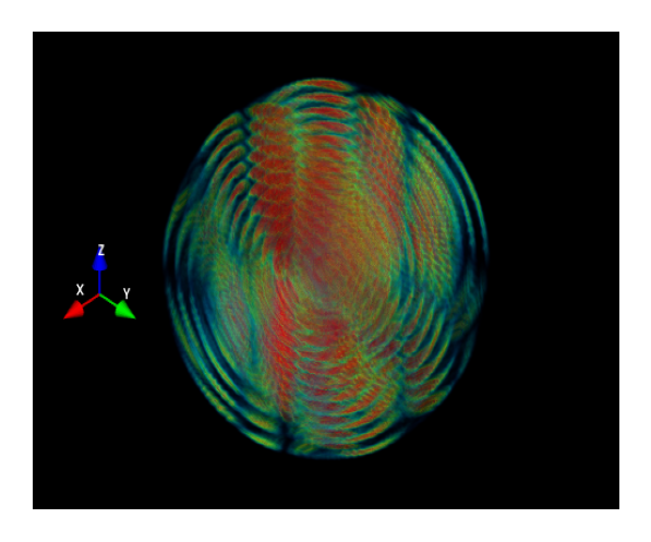
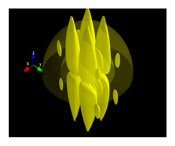
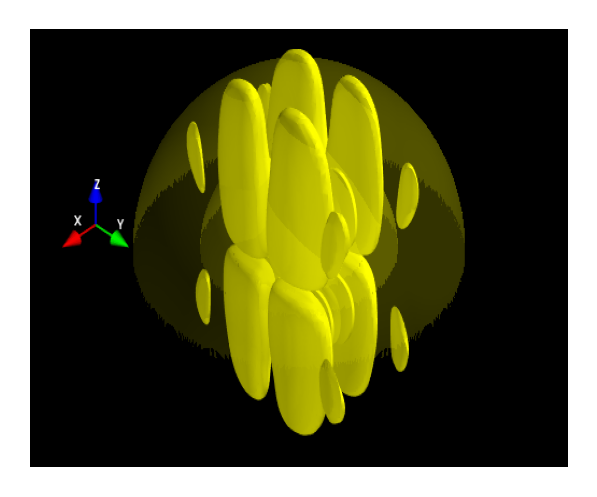
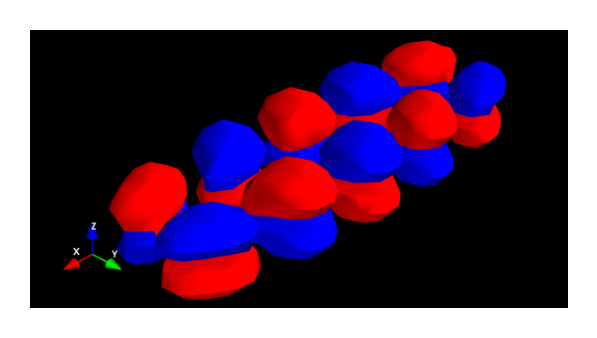
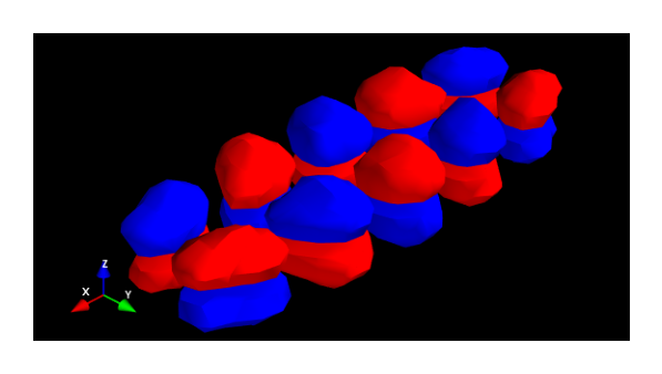
Figure 1: a) Data obtained from ARPES; b) Fourier amplitude of the exact solution; c) Fourier amplitude of reconstruction at smallest gap of the CDR$\lambda$ with $\lambda=0.7$; d) The exact solution; e) Reconstruction at smallest gap of the CDR$\lambda$ with $\lambda=0.7$.

In Figure 2(a), we present five examples of convergence plots for the cyclic projection and the cyclic relaxed Douglas-Rachford methods ($\lambda=0.3$ and $\lambda=0.7$) starting from the same initializations. Once a local region of convergence has been found, the algorithm converges linearly to a tolerance $\text{tol}=10^{-8}$. The theory behind these methods, whether cyclic projections or Douglas-Rachford, does not state how long one has to wait before a local region of convergence is found (i.e. there is no global theory). The slopes of the convergence plots for cyclic projections are always steeper than those of the cyclic Douglas-Rachford, indicating that the former has a better rate of linear convergence. Over 100 trials, the cyclic projection method reaches the tolerance in an average of 169 iterations, while the cyclic relaxed Douglas-Rachford method requires more time, averaging 336 iterations. If we reduce $\lambda$ to $0.3$, the average number of iterations is reduced to $280$. This can be explained based on the operator: as $\lambda\to 0$, the relaxation term is smaller, and the cyclic relaxed Douglas-Rachford operator approaches the cyclic projection operator. In Figure 2(b), we illustrate the relationship between the gap (3.2) and the error (24) at final iterates for the two algorithms, where the error represents the difference between the approximate fixed point and the exact solution (see [9]). We observe that: 1) a smaller gap indicates better reconstruction, and 2) the approximate fixed points of the cyclic relaxed Douglas-Rachford have gaps and errors that are roughly the same as those of the fixed points of the cyclic projection. These observations further support the statement that the gap is reliable and that the shadow of the fixed points of the cyclic relaxed Douglas-Rachford on the set SYM is close to the fixed points of the cyclic projection, as stated in Section 3.4.2.

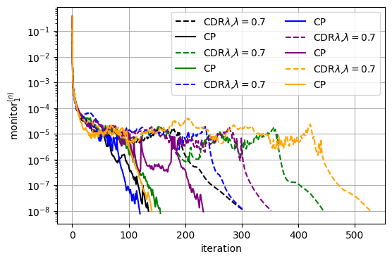
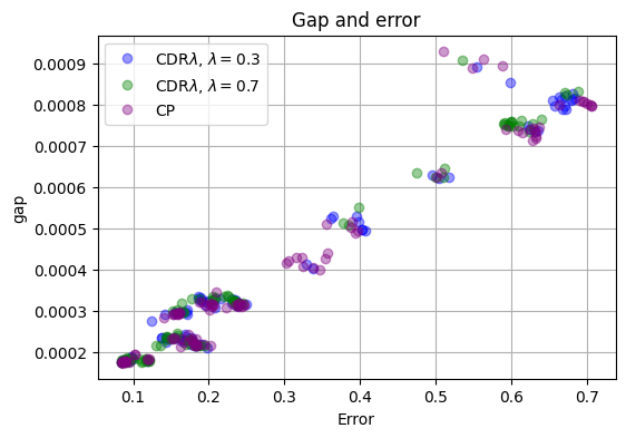
Figure 2: (a) Five “typical” convergence plots of the cyclic relaxed Douglash-Rachford and cyclic projection algorithms. (b) The relationship between gap and error at (approximate) fixed points of the two algorithms.

We now compare the efficiency of the two methods.

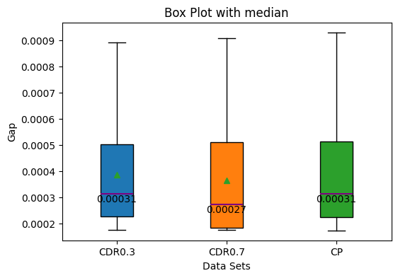
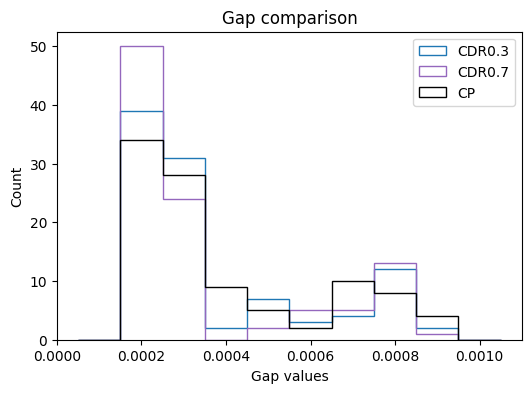
Figure 3: CP and CDR$\lambda$, $\lambda=0.7,0.3$ with 100 trials for each method. (a) Boxplots showing gap variation. (b) Histogram of the gap.

Figure 3(a) shows the median, mean, variance, maximum and minimum of the gaps of the final iterates of the cyclic projections and cyclic relaxed Douglas-Rachford algorithms ($\lambda=0.3$ and $\lambda=0.7$). The minimum achieved gap for all three numerical experiments is the same, but the mean, variance and maximum gaps are slightly different, indicating that CDR$\lambda$ with $\lambda=0.7$ achieves (slightly) better results on average. This is also shown in the histogram Figure 3(b) of gap values obtained by the three. We divide the approximate fixed points into 8 clusters and see that the cyclic relaxed Douglas-Rachford achieves a higher frequency of small gap values compared to the cyclic projection for each value of $\lambda$. In the cluster with the smallest gap values, while the cyclic projection algorithm finds this cluster only 34% of the time, the cyclic relaxed Douglas-Rachford finds this cluster for both values of $\lambda$, reaching up to 50% at $\lambda=0.7$. These results demonstrate that the cyclic relaxed Douglas-Rachford algorithm has a greater ability to achieve a higher success rate than the cyclic projection, which is considered state-of-the-art in [9]. This capability depends on the relaxation parameter $\lambda$, which can be fine-tuned.

We have already seen that adjusting the value of the parameter $\lambda\in[0,1]$ increases the likelihood of obtaining good reconstructions for cyclic relaxed Douglas-Rachford. However, the ability to avoid poor local minima remains unremarkable. We compare both CP and CDR$\lambda$ to the relaxed Douglas-Rachford on the product space (18).

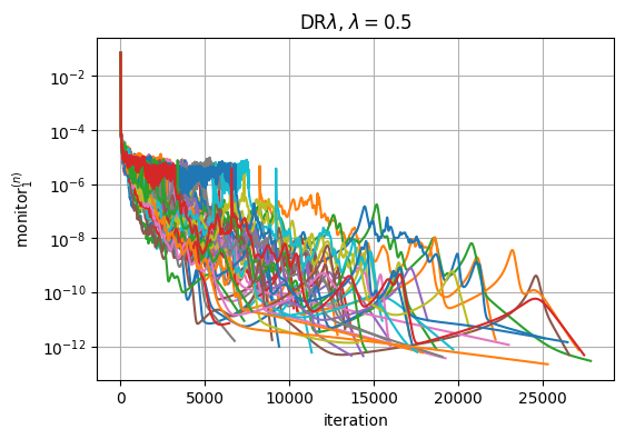
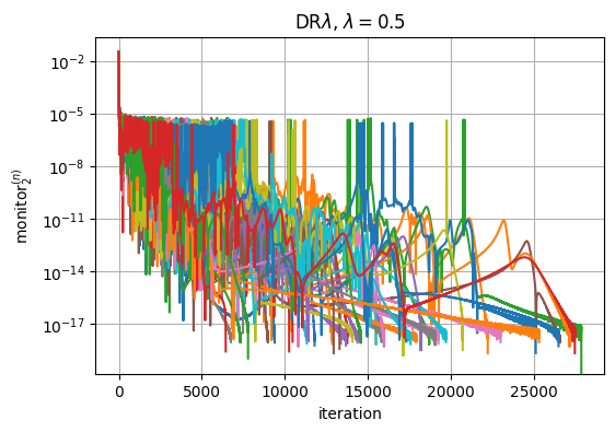
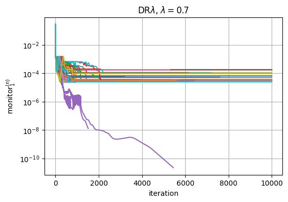
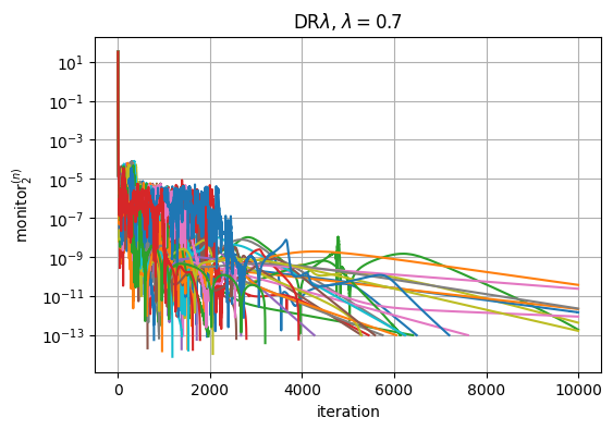
Figure 4: DR$\lambda$. Convergence plots of changes (monitor₁, left column) and gaps (monitor₂, right column) for the algorithm with two values of $\lambda$. Each $\lambda$ was run with 50 different starting points.

We begin by discussing the convergence since the convergence behavior of DR$\lambda$ on the product space is qualitatively different than CP or CDR$\lambda$.

Starting from a fixed, randomly selected initial point and examining the behavior of DR$\lambda$ for different values of $\lambda\in(0,1)$, we observe that the convergence of this algorithm depends, as expected, on the value of $\lambda$. When $\lambda\leq 0.5$, the iterate difference, $\text{monitor}^{(n)}_{1}$, converges linearly, as expected. However, significantly more iterations are required to observe this convergence: on the order of $20000$ iterations compared to less than $500$ iterations for all of the cyclic methods.

When $0.5<\lambda<0.8$, we observe that $\text{monitor}^{(n)}_{1}$ lies on spheres centered at $0$, with a constant radius $r\approx\|P_{\text{SYM}}u^{(n)}-P_{\text{SYM}}u^{(n-1)}\|$ as $n$ approaches infinity. Despite that, we see the convergence of the difference gap, i.e., $\text{monitor}^{(n)}_{2}$ in both situations. To confirm these behaviors, we run the algorithm with two values, $\lambda=0.5$ and $\lambda=0.7$. Each $\lambda$ is tested with 50 trials, using the same starting points for both values. Figure 4 confirms the initial observations more definitively. For $\lambda=0.5$, the changes in all the trials converge linearly, whereas with $\lambda=0.7$, only one of them converges, see Figures 4(a) and (c). On the contrary, the gaps converge well, see 4(b) and (d). Note that in these two experiments, we set a tolerance of $5\times 10^{-18}$ and $n_{\max}=35000$ for $\lambda=0.5$ and $1\times 10^{-13}$ and $n_{\max}=10000$ for $\lambda=0.7$, as this tolerance and maximum iteration are sufficient to observe linear convergence.

Figure 5 presents the results of the cyclic projection and relaxed Douglas-Rachford methods with the two different values of $\lambda$ for 50 trials. The (approximate) fixed points of CP and DR$\lambda$ on the product space with $\lambda=0.5$ seem distributed across many clusters. With this value of $\lambda$, the results of the two algorithms appear to be similar, but the latter algorithm still excels at finding smaller gaps. With $\lambda=0.7$, however, DR$\lambda$ on the product space is much more robust, with most (approximate) fixed points moving to the lowest cluster, where the gap and error are smaller. In addition to the above experiments, we conducted 50 more trials for the relaxed Douglas-Rachford method, but now the starting points are the 50 (approximate) fixed points of the algorithm with $\lambda=0.5$. Figure 5(b) shows the results. Despite different initial starting points, the algorithm tends to converge to good clusters, i.e., it returns good reconstructions. This demonstrates the stability of the algorithm. These findings conclude that DR$\lambda$ on the product space reliably avoids poor local minima when an appropriate value of the parameter $\lambda$ is chosen. As characterized in Section 3.4.2, the set of fixed points of DR$\lambda$ on the product space is monotone decreasing as $\lambda$ increases. Though the characterization of the fixed points does not imply that the smaller fixed point set necessarily corresponds to better local minima, Figure 5 demonstrates this dramatically, showing that the smaller fixed point set for $\lambda=0.7$ corresponds to points with smaller gaps, and errors.

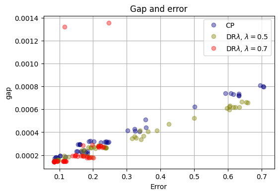
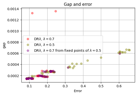
Figure 5: (a) Comparison of the efficiency between cyclic projection and relaxed Douglas-Rachford with $\lambda=0.5$ and $\lambda=0.7$. (b) Stabilization of approximate fixed points of relaxed Douglas-Rachford, with $\lambda=0.7$, starting from random initialization, and the approximate fixed points of the relaxed Douglas-Rachford with $\lambda=0.5$.

4.2 Experimental Data

We perform numerical comparisons on the experimental dataset presented in [2]. All sets and parameters from [3] are retained here. Since the ground truth is unknown, we compare the gap sizes for fixed points of the cyclic projection algorithm with the gaps achieved by the product space formulation of the relaxed Douglas-Rachford method, initialized from the fixed points of CP.

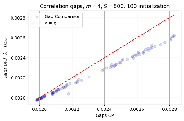
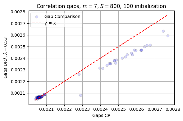
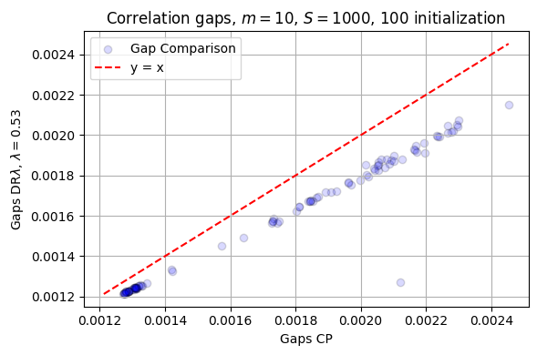
Figure 6: Comparison of the quality of fixed points between cyclic projections and product space formulation of the relaxed Douglas-Rachford algorithm with $\lambda=0.53$. The points show the gap sizes achieved by DR$\lambda$ (y-axis) when initialized from the fixed points of CP (gap size shown on the x-axis).

Figure 6 shows the correspondence of the gapsizes for the two methods using 4, 7 and 10 data spheres, denoted as $m$. We run the CP algorithm with 100 initializations and subsequently start the product space DR$\lambda$ algorithm from the corresponding 100 fixed points of the CP algorithm, with $\lambda=0.53$ in each case. This parameter was found by trial and error and yielded the best results for the method. If a point lies on the red diagonal lines, it indicates that the DR$\lambda$ algorithm did not improve the gap over what was already achieved by the CP algorithm. In all three plots, however, we observe that all 100 points lie below the diagonal, indicating that the relaxed Douglas-Rachford method always achieves a smaller gap than the cyclic projection. Furthermore, the DR$\lambda$ gap tends to decrease more sharply as the CP gap increases, suggesting that applying DR$\lambda$ after CP will have a more significant impact for problems with a relatively broad distribution of fixed points. Interestingly, and quite unexpected, the experimental data appears to lead to a feasibility problem with a comparatively small range of fixed point gaps relative to the simulated data in the previous section. In other words, the experimental data set is more regular than our simulated data set. This apparent regularity of the experimental data can be understood as, perhaps, an averaging due to noise which eliminates regions with a large gap, understood as extreme local minima. This makes intuitive sense in light of the characterization of the fixed points of the DR$\lambda$ algorithm given in (67): fixed points associated with large gaps should be less stable. The difference between the structures reconstructed from the CP fixed points and those reconstructed from the subsequent DR$\lambda$ fixed points are most of the time not distinguishable physically for this data (see Figure 7(b)-(c)). As shown in Figure 6(b)-(c), however, in a small number of instances, the DR$\lambda$ algorithm can shift the CP fixed point to a significantly different structure. This is demonstrated in 7(d)-(e).

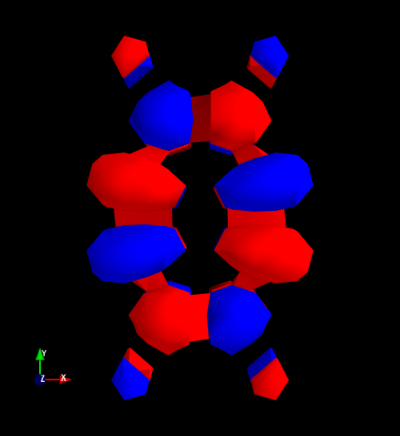
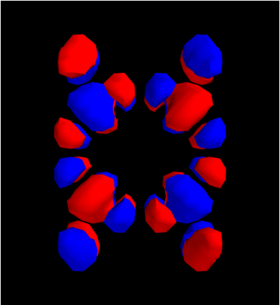
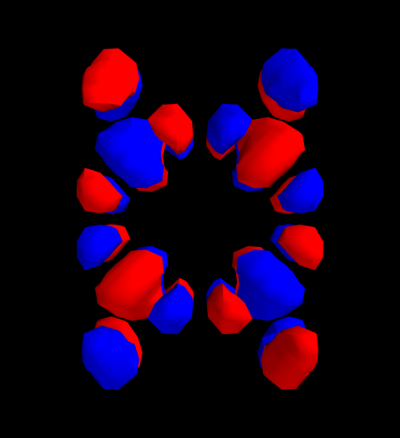
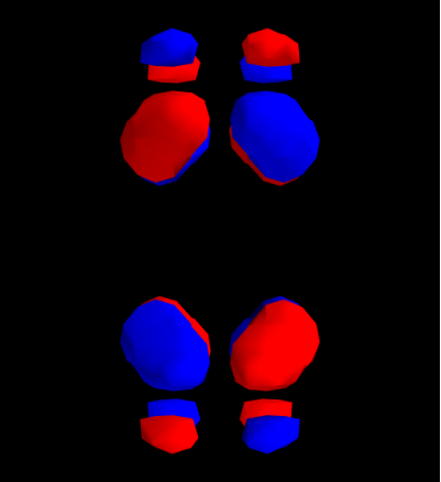
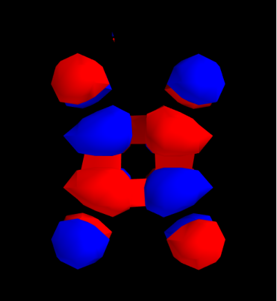
Figure 7: Examples of reconstructions using 10 data spheres. (a) A reconstruction with a small gap corresponding to a physically expected structure. (b) Reconstruction at a fixed point of CP with a large gap. (c) Reconstruction at the fixed point of DR$\lambda$ ($\lambda=0.53$) initialized from the CP fixed point shown in (b). (d) Reconstruction at a fixed point of CP with a large gap (gap=$0.00212$). (e) Reconstruction at the fixed point of DR$\lambda$ (gap=$0.00127$) initialized from the CP fixed point shown in (d).

5 Conclusion

The cyclic relaxed Douglas-Rachford method was first proposed in [18] as an alternative to the classical cyclic projections and the more recent cyclic Douglas-Rachford algorithms. The hope for this algorithm was that it would more reliably find “higher quality” fixed points than the other methods. We characterized the fixed points in [8], but the potential of this algorithm for filtering out bad local minima was not tested until this numerical study. The results do confirm the initial motivation for this algorithm, but not dramatically. Quite surprisingly, however, we found that the relaxed Douglas-Rachford algorithm on the product space, while exhibiting quite poor convergence rates, does an excellent job of filtering out bad local minima from all cyclic algorithms. Both the product space and cyclic implementations of the Douglas-Rachford algorithm require significantly more iterations to find fixed points than the cyclic projections algorithm. This is to be expected, since the iterates of the relaxed Douglas-Rachford algorithm, for a large enough relaxation parameter, will be dispersed across a broader region of the domain than cyclic projections. Our numerical experiments therefore lead to the following recommendation: run cyclic projections to find some fixed point, and from this fixed point run DR$\lambda$ on the product space formulation of the problem with as large a value of $\lambda$ as is numerically stable, in order to move toward a fixed point with smaller gaps between the constraint sets. This advice is counter to the current practice for phase retrieval, where the Douglas-Rachford algorithm (known in the physics community as the Fienup Hybrid-Input-Output algorithm) is run for several iterations, and then cyclic projections (known as Gerchberg-Saxton or error reduction methods) is used to “clean up” the images [15].

References

- [1] H. H. Bauschke, D. R. Luke, H. M. Phan, and X. Wang. Restricted normal cones and sparsity optimization with affine constraints. Found. Comput. Math., 14:63–83, 2014.
- [2] W. Bennecke, T. L. Dinh, J. P. Bange, D. Schmitt, M. Merboldt, L. Weinhagen, B. van Wingerden, F. Frassetto, L. Poletto, M. Reutzel, D. Steil, D. R. Luke, S. Mathias, and G. S. M. Jansen. Table-top three-dimensional photoemission orbital tomography with a femtosecond extreme ultraviolet light source. arXiv preprint, February 2025, http://arxiv.org/abs/2502.12285.
- [3] W. Bennecke, T. L. Dinh, J. P. Bange, D. Schmitt, M. Merboldt, L. Weinhagen, B. van Wingerden, F. Frassetto, L. Poletto, M. Reutzel, D. Steil, D. R. Luke, S. Mathias, and G. S. M. Jansen. Replication Data for: Table-top three-dimensional photoemission orbital tomography with a femtosecond extreme ultraviolet light source, 2025, https://doi.org/10.25625/1EMFFL.
- [4] A. Bërdëllima, F. Lauster, and D. R. Luke. -firmly nonexpansive operators on metric spaces. J. Fixed Point Theory Appl., 24(1):14, 2022.
- [5] J. M. Borwein and M. K. Tam. A cyclic Douglas-Rachford iteration scheme. J. Optim. Theory Appl., 160(1):1–29, 2014.
- [6] M. N. Dao and H. M. Phan. Linear convergence of the generalized Douglas-Rachford algorithm for feasibility problems. J. Glob. Optim., 72(3):443–474, 2018.
- [7] J. E. Dennis and R. Schnabel. Numerical Methods for Unconstrained Optimization and Nonlinear Equations. Prentice Hall, Englewood Cliffs, NJ, 1996.
- [8] T. L. Dinh, G. S. M. Jansen, and D. R. Luke. The Cyclic Relaxed Douglas-Rachford Algorithm for Inconsistent Nonconvex Feasibility. arXiv preprint, 2025, http://arxiv.org/abs/2502.12285.
- [9] T. L. Dinh, G. S. M. Jansen, D. R. Luke, W. Bennecke, and S. Mathias. A minimalist approach to 3d photoemission orbital tomography: algorithms and data requirements. New Journal of Physics, 26(4):043024, apr 2024.
- [10] N. Hermer, D. R. Luke, and A. Sturm. Rates of convergence for chains of expansive Markov operators. Trans. Math. Appl., 7(1):tnad001, 12 2023.
- [11] R. Hesse and D. R. Luke. Nonconvex notions of regularity and convergence of fundamental algorithms for feasibility problems. SIAM J. on Optim., 23(4):2397–2419, 2013.
- [12] R. Hesse, D. R. Luke, and P. Neumann. Alternating projections and Douglas–Rachford for sparse affine feasibility. IEEE Trans. Signal. Process., 62(18):4868–4881, 2014.
- [13] G. Li and T. K. Pong. Douglas–Rachford splitting for nonconvex optimization with application to nonconvex feasibility problems. Math. Program., 159(1-2):371–401, 2016.
- [14] D. R. Luke. Finding best approximation pairs relative to a convex and a prox-regular set in Hilbert space. SIAM J. Optim., 19(2):714–739, 2008.
- [15] D. R. Luke. Phase retrieval, what’s new? SIAG/OPT Views and News, 25(1):1–5, 2017.
- [16] D. R. Luke, J. V. Burke, and R. G. Lyon. Optical wavefront reconstruction: Theory and numerical methods. SIAM Review, 44(2):169–224, 2002.
- [17] D. R. Luke and A.-L. Martins. Convergence Analysis of the Relaxed Douglas–Rachford Algorithm. SIAM J. on Optim., 30(1):542–584, 2020.
- [18] D. R. Luke, A.-L. Martins, and M. K. Tam. Relaxed cyclic Douglas-Rachford algorithms for nonconvex optimization. In Proceedings of the ICML Workshop: Modern Trends in Nonconvex Optimization for Machine Learning, Stockholm, July 2018. ICML.
- [19] D. R. Luke, S. Sabach, and M. Teboulle. Optimization on spheres: models and proximal algorithms with computational performance comparisons. SIAM J. Math. Data Sci., 1(3):408–445, 2019.
- [20] D. R. Luke, N. H. Thao, and M. K. Tam. Quantitative convergence analysis of iterated expansive, set-valued mappings. Math. Oper. Res., 43(4):1143–1176, 2018.
- [21] H. Phan. Linear convergence of the Douglas–Rachford method for two closed sets. Optimization, 65(2):369–385, 2016.
- [22] G. Pierra. Decomposition through formalization in a product space. Math. Program., 28:96–115, 1984.
- [23] R. Poliquin, R. Rockafellar, and L. Thibault. Local differentiability of distance functions. Trans. Amer. Math. Soc., 352(11):5231–5249, 2000.
- [24] N. H. Thao. A convergent relaxation of the Douglas–Rachford algorithm. Comput. Optim. Appl., 70(3):841–863, 2018.
- [25] J. von Neumann. Functional Operators, Vol II. The geometry of orthogonal spaces, volume 22 of Ann. Math Stud. Princeton University Press, 1950. Reprint of mimeographed lecture notes first distributed in 1933.