Empirical likelihood approach for high-dimensional moment restrictions with dependent data

Abstract

Economic and financial models—such as vector autoregressions, local projections, and multivariate volatility models—feature complex dynamic interactions and spillovers across many time series. These models can be integrated into a unified framework, with high-dimensional parameters identified by moment conditions. As the number of parameters and moment conditions may surpass the sample size, we propose adding a double penalty to the empirical likelihood criterion to induce sparsity and facilitate dimension reduction. Notably, we utilize a marginal empirical likelihood approach despite temporal dependence in the data. Under regularity conditions, we provide asymptotic guarantees for our method, making it an attractive option for estimating large-scale multivariate time series models. We demonstrate the versatility of our procedure through extensive Monte Carlo simulations and three empirical applications, including analyses of US sectoral inflation rates, fiscal multipliers, and volatility spillover in China’s banking sector.

keywords: $\alpha$-mixing, asymptotic analysis, confidence region, high dimensionality, penalized likelihood

1 Introduction

Econometrics began almost a hundred years ago with a focus on deciphering business cycles and economic fluctuations, as demonstrated by early researchers Fisher (1925), Frisch (1933), and Tinbergen (1939). These pioneers carried out their quantitative analyses with limited macro-level, low-frequency datasets. However, with the progress in information technology, economists now have access to extensive long-term data series that reflect the state of real economies and financial markets from diverse angles. Despite this, the complexity of the economic landscape continues to escalate, characterized over the last century by exceptional growth interspersed with recessions, wars, and crises. The age-old inquiry into the interplay between economic variables and their evolving paths still holds a prominent place in the current big data era.

An important class of economic models is characterized by moment conditions. To fix ideas, let $\{{\mathbf{x}}_{t}\}_{t=1}^{n}$ be $d$-dimensional random vectors, and $\boldsymbol{\theta}=(\theta_{1},\ldots,\theta_{p})^{{\mathrm{\scriptscriptstyle\top}}}$ be a $p$-dimensional parameter in a parameter space $\boldsymbol{\Theta}$. For an $r$-dimensional estimating function ${\mathbf{g}}({\mathbf{x}};\boldsymbol{\theta})=\{g_{1}({\mathbf{x}};\boldsymbol{\theta}),\dots,g_{r}({\mathbf{x}};\boldsymbol{\theta})\}^{\mathrm{\scriptscriptstyle\top}}$, the information for the true parameter $\boldsymbol{\theta}_{0}$ is identified by the moment condition

$$\mathbb{E}\{{{\mathbf{g}}({\mathbf{x}}_{t};\boldsymbol{\theta}_{0})}\}={\bf 0}$$ (1)

for each $t=1,\ldots,n$. In the traditional asymptotic analysis, it is assumed that the sample size $n$ approaches infinity while the model remains unchanged. Economic theory, however, often relies on the orthogonality of variables as a justification for moment conditions, but it generally lacks clarity regarding which variables should be included or which moment conditions should be utilized. For example, Angrist and Krueger (1991) and Eaton et al. (2011) involve a large number of moments, and Blundell et al. (1993) and Fan and Liao (2014) further contain many parameters. Beyond these applications in labor economics, international trade, and household consumption, multivariate time series models provide fertile ground for the development of complex economic models.

This study is driven by three commonly utilized multivariate time series models, as detailed in Lütkepohl (2005)’s monograph. First, the vector autoregressive (VAR) model (Sims 1980) is a multivariate extension of the univariate autoregressive (AR) model. In a VAR model composed of $d$ variables, the total number of slope coefficients is $p=O(d^{2})$. This is referenced as our Example 1 in Section 5. Conventionally, the VAR model only includes a limited number of variables, which is not designed to handle a modern large system of variables.

The second example is concerning the impulse response function (IRF), which describes the effect of an external shock to a target variable. IRF is a key object of macroeconomic interest; see the survey by Nakamura and Steinsson (2018). Traditionally, IRF is implied by a fully and “correctly specified” VAR model. Recently, Jordà (2005) introduced local projection (LP), a much simpler method which involves a series of single-equation regressions over the forecast horizons $h=0,1,\ldots,H$. If each individual regression includes $d$ regressors, the system yields $p=d(H+1)$ slope coefficients to be estimated.

In addition to the above two examples of conditional mean models, volatility is fundamental for financial risk management. The most recognized univariate time series volatility models are the autoregressive conditional heteroskedasticity (ARCH) model (Engle 1982) and its generalized version (GARCH) (Bollerslev 1986). In typical financial markets, numerous assets are traded daily. To handle this complexity, multivariate volatility models, such as the multivariate ARCH (MARCH) and multivariate GARCH (MGARCH) (Engle and Kroner 1995), have been developed. As will be explained in Example 3 in Section 5, these models require high-dimensional coefficients to capture the interdependencies among various assets.

Moment restrictions serve as a comprehensive framework for identifying the parameters of interest across all the above-mentioned three multivariate time series models. Within the context of these moment constraints, the generalized method of moments (GMM) is widely regarded as the default econometric estimation approach (Hansen 1982, Hansen and Singleton 1982). Although Hansen’s two-step GMM achieves asymptotic efficiency under the traditional asymptotic scenario with fixed $r$ and $p$, its performance in finite samples can be unsatisfactory, as is highlighted by Altonji and Segal (1996). This issue primarily arises from the inversion of the estimated covariance matrix of the estimating functions. Recently, Cheng et al. (2023) investigate the bias of GMM in cases where $p$ is proportional to, but smaller than $n$. When $p$ exceeds $n$, Belloni et al. (2018) propose using a sup-norm objective criterion function to manage many moments, departing from GMM’s quadratic form.

An alternative to GMM is empirical likelihood (EL) (Owen 1988, Qin and Lawless 1994), which can be viewed through the lens of information theory (Kitamura and Stutzer 1997). Unlike methods that require explicit computation of the covariance matrix of the estimating functions, EL benefits from reduced variance due to higher-order enhancements (Newey and Smith 2004). When dealing with models incorporating many moments, the EL criterion function can be augmented with a penalized approach to regularize both the multitude of moments and high-dimensional coefficients. This branch of theoretical properties, specifically for independently and identically distributed (i.i.d.) observations, has been extended by Otsu (2007), Leng and Tang (2012), Shi (2016), and Chang et al. (2018). Penalized method theory is relatively straightforward with i.i.d. data. To our knowledge, this paper is the first to explore the EL methodology in the context of high-dimensional temporally dependent data.

In classical low-dimensional settings, Kitamura (1997) advocates using blocks of time series observations in EL to preserve the temporal dependence and recover the Wilks’ phenomenon. This blocking technique is employed by Chang et al. (2015) under a moderately high-dimensional environment where $r/n\to 0$. However, the blocking technique is inconvenient when dealing with high-dimensionality in both the parameters and moments. This paper maintains the simplest approach: treating the EL as if the data is i.i.d., which can be interpreted as the marginal EL for time series. Though marginal likelihood estimation has been used in low-dimensional models (Levenbach 1972) and has been applied in financial applications (Stambaugh 1997, Patton 2006) for integration of varying lengths, this paper is the first to investigate the scheme of marginalization in the framework of EL for time series, distinct from the approaches by Chang et al. (2013; 2016).

We establish rigorous asymptotic theory for the penalized EL (PEL) with many parameters and many moments under time dependence of $\alpha$-mixing. To accommodate stronger temporal dependence, we introduce (in Condition 1) a diverging quantity $L_{n}$ within the $\alpha$-mixing coefficient. To address the high-dimensional challenges in this framework, we bound the tail probabilities of certain key statistics by novel inequalities, which are constructed via self-normalized sum inequalities (Jing et al. 2003). We show that under sparsity conditions, the PEL approach delivers consistent estimation, and the resulting PEL estimator is asymptotically normally distributed. For investigations focused on a low-dimensional parameter, we further employ a projected PEL (PPEL) method (Chang et al. 2021) to eliminate the bias induced by the high-dimensional nuisance parameters, thereby reinstating the usual inference method using the $t$-statistic.

This procedure enables the application of the method to a wide range of multivariate time series models with many parameters, including VAR, LP, and MARCH/MGARCH models as discussed. Extensive Monte Carlo simulations show that our method performs well in finite sample. We employ it to further study the persistence and spillover of the USA’s sectoral inflation, the magnitude of the fiscal multiplier, and the volatility network of China’s banking industry.

This paper stands on the large literature of time series, empirical likelihood, and high-dimensional estimation. It leverages the penalized estimation in Chang et al. (2018) and Chang et al. (2021), developed under the i.i.d. setting. These steps are carried over and adapted to the environment with temporal dependence. Compared to the GMM-type alternative, Belloni et al. (2018) is developed in the i.i.d. environment, which is critical for their sample splitting; sample splitting in time series is much more challenging and may adversely affect finite sample performance when the time length is moderate in practice. On the other hand, the literature of high-dimensional time series has witnessed specific proposals for standalone models. For example, Shi et al. (2024) and Mei and Shi (2024) focus on high-dimensional time series dense regressions and sparse regressions, respectively. Under the assumption of Gaussian errors, Kock and Callot (2015) develop Lasso-type penalized estimation for VAR models. Caner and Kock (2018) attack high-dimensional GMM-type models, where their linear setting facilitates the estimation of the large weighting matrix. Adamek et al. (2024) provide theory for a single-equation regression with many covariates for local projection, and deal with ridge-type regularization in fixed dimension. Our procedure provides a unified framework to handle models defined by moment conditions.

The rest of the paper is organized as follows. Section 2 sets up the model and the technical conditions. The consistency and asymptotic distribution of the PEL estimator are established in Section 3, and the asymptotic normality of PPEL is presented in Section 4. We carry out Monte Carlo simulations in Section 5, and showcase our method in three empirical applications in Section 6. The code and data are available at the GitHub repository: https://github.com/JinyuanChang-Lab/PenalizedELwithDependentData. All proofs are relegated to the Appendices.

Notation. We use the abbreviations “w.p.a.1” and “w.r.t” to denote, respectively, with probability approaching one and with respect to. For any real number $x$, define $\lfloor x\rfloor=\max\{q\in\mathbb{Z}:q\leq x\}$, where $\mathbb{Z}$ denotes the set of all integers. For two sequences of positive numbers $\{a_{n}\}$ and $\{b_{n}\}$, we write $a_{n}\lesssim b_{n}$ or $b_{n}\gtrsim a_{n}$ if there exists a positive constant $c$ such that $\lim\sup_{n\to\infty}a_{n}/b_{n}\leq c$, and $a_{n}\asymp b_{n}$ if and only if $a_{n}\lesssim b_{n}$ and $b_{n}\lesssim a_{n}$ hold simultaneously. We write $a_{n}\ll b_{n}$ or $b_{n}\gg a_{n}$ if $\lim\sup_{n\to\infty}a_{n}/b_{n}=0$. Let “vec” and “vech” be the vector operators that stack the columns of a matrix and the upper triangular part of a matrix, respectively, into a vector. For a positive integer $q$, we write $[q]=\{1,\ldots,q\}$, and let ${\mathbf{I}}_{q}$ be the $q\times q$ identity matrix. For a $q\times q$ symmetric matrix ${\mathbf{Q}}$, denote by $\lambda_{\min}({\mathbf{Q}})$ and $\lambda_{\max}({\mathbf{Q}})$ the smallest and largest eigenvalues of ${\mathbf{Q}}$, respectively. For a $q_{1}\times q_{2}$ matrix ${\mathbf{B}}=(b_{i,j})_{q_{1}\times q_{2}}$, let ${\mathbf{B}}^{{\mathrm{\scriptscriptstyle\top}}}$ be its transpose, $|{\mathbf{B}}|_{\infty}=\max_{i\in[q_{1}],j\in[q_{2}]}|b_{i,j}|$ be the sup-norm, and $\|{\mathbf{B}}\|_{2}=\lambda_{\max}^{1/2}({\mathbf{B}}^{\otimes 2})$ be the spectral norm with ${\mathbf{B}}^{\otimes 2}={\mathbf{B}}{\mathbf{B}}^{{\mathrm{\scriptscriptstyle\top}}}$. Specifically, when $q=1$, we use $|{\mathbf{B}}|_{1}=\sum_{i=1}^{q_{1}}|b_{i,1}|$ and $|{\mathbf{B}}|_{2}=(\sum_{i=1}^{q_{1}}b_{i,1}^{2})^{1/2}$ to denote the $L_{1}$-norm and $L_{2}$-norm of the vector ${\mathbf{B}}$. For two square matrices ${\mathbf{Q}}_{1}$ and ${\mathbf{Q}}_{2}$, we say ${\mathbf{Q}}_{1}\leq{\mathbf{Q}}_{2}$ if $({\mathbf{Q}}_{2}-{\mathbf{Q}}_{1})$ is a positive semi-definite matrix. The population mean is denoted by $\mathbb{E}(\cdot)$, and the sample mean is denoted by $\mathbb{E}_{n}(\cdot)=n^{-1}\sum_{t=1}^{n}(\cdot)$. For a given index set $\mathcal{L}$, let $|\mathcal{L}|$ be its cardinality. For a generic multivariate function ${\mathbf{h}}(\cdot;\cdot)$, we denote by ${\mathbf{h}}_{{\mathcal{\scriptscriptstyle L}}}(\cdot;\cdot)$ the subvector of ${\mathbf{h}}(\cdot;\cdot)$ collecting the components indexed by $\mathcal{L}$. Analogously, we write ${\mathbf{a}}_{\mathcal{L}}$ as the corresponding subvector of a vector ${\mathbf{a}}$. For simplicity and when no confusion arises, we use the generic notation ${\mathbf{h}}_{t}(\boldsymbol{\theta})$ as equivalent to ${\mathbf{h}}({\mathbf{x}}_{t};\boldsymbol{\theta})$, and $\nabla_{\boldsymbol{\theta}}{\mathbf{h}}_{t}(\boldsymbol{\theta})$ for the first-order partial derivative of ${\mathbf{h}}_{t}(\boldsymbol{\theta})$ w.r.t $\boldsymbol{\theta}$. Denote by $h_{t,k}(\boldsymbol{\theta})$ the $k$-th component of ${\mathbf{h}}_{t}(\boldsymbol{\theta})$. Let $\bar{{\mathbf{h}}}(\boldsymbol{\theta})=\mathbb{E}_{n}\{{\mathbf{h}}_{t}(\boldsymbol{\theta})\}$, and write its $k$-th component as $\bar{h}_{k}(\boldsymbol{\theta})=\mathbb{E}_{n}\{h_{t,k}(\boldsymbol{\theta})\}$. Analogously, let ${\mathbf{h}}_{t,{\mathcal{\scriptscriptstyle L}}}(\boldsymbol{\theta})={\mathbf{h}}_{{\mathcal{\scriptscriptstyle L}}}({\mathbf{x}}_{t};\boldsymbol{\theta})$ and $\bar{{\mathbf{h}}}_{{\mathcal{\scriptscriptstyle L}}}(\boldsymbol{\theta})=\mathbb{E}_{n}\{{\mathbf{h}}_{t,{\mathcal{\scriptscriptstyle L}}}(\boldsymbol{\theta})\}$.

2 Preliminaries

In this paper, we build up our theory with $\alpha$-mixing time dependence. Let $\mathcal{F}_{-\infty}^{u}$ and $\mathcal{F}_{u}^{\infty}$ be the $\sigma$-fields generated by $\{{\mathbf{x}}_{t}\}_{t\leq u}$ and $\{{\mathbf{x}}_{t}\}_{t\geq u}$, respectively. The $\alpha$-mixing coefficient of the sequence $\{{\mathbf{x}}_{t}\}$ at lag $k$ is defined as

$$\alpha_{n}(k):=\sup_{t}\sup_{A\in\mathcal{F}_{-\infty}^{t},\,B\in\mathcal{F}_{t+k}^{\infty}}|\mathbb{P}(A\cap B)-\mathbb{P}(A)\mathbb{P}(B)|$$ (2)

for each $k\geq 1$. The notion of $\alpha$-mixing in $\eqref{eq:alpha-mixing}$ broadly characterizes serial dependence. Specifically, we impose the following assumption as in Chang et al. (2024a) in our study.

Condition 1.

$\{{\mathbf{x}}_{t}\}_{t=1}^{n}$ is an $\alpha$-mixing sequence, and there exist some universal constants $K_{1}>1$, $K_{2}>0$ and $\varphi\geq 1$ such that $\alpha_{n}(k)\leq K_{1}\exp\{-K_{2}(L_{n}^{-1}k)^{\varphi}\}$ for any $k\geq 1$, where $L_{n}>0$ can stay finite or diverge to infinity with $n$.

Condition 1 does not require $\{{\mathbf{x}}_{t}\}_{t=1}^{n}$ to be strictly stationary. For an independent sequence $\{{\mathbf{x}}_{t}\}_{t=1}^{n}$, we can select $L_{n}=1/2$ and $\varphi=\infty$. For an $L_{n}$-dependent sequence $\{{\mathbf{x}}_{t}\}_{t=1}^{n}$, we can select $\varphi=\infty$. A variety of time series models that are routinely used in economics and finance are covered by Condition 1. For example, under some regularity conditions, the autoregressive-moving-average (ARMA) processes, the stationary Markov chains (Fan and Yao 2003), and the stationary GARCH models (Carrasco and Chen 2002) satisfy $\alpha$-mixing with the exponentially decaying coefficient ($L_{n}=1$ and $\varphi=1$). This condition further covers their multivariate generalizations of VAR and MGARCH (MGARCH includes MARCH as a special case); see Hafner and Preminger (2009), Boussama et al. (2011) and Wong et al. (2020).

The quantity $L_{n}$ involved in Condition 1 accommodates practical scenarios of big data collected over time. Write ${\mathbf{x}}_{t}=(x_{t,1},\ldots,x_{t,d})^{{\mathrm{\scriptscriptstyle\top}}}$. Consider the simple case when each univariate time series $\{x_{t,i}\}_{t=1}^{n}$ for $i\in[d]$ is $\alpha$-mixing with exponentially decaying $\alpha$-mixing coefficients, while those $d$ sequences are mutually independent. Theorem 5.1 of Bradley (2005) indicates that $\alpha_{n}(k)$ defined in (2) satisfies $\alpha_{n}(k)\leq d\exp(-ck)$ for some universal constant $c>0$, which implies Condition 1 holds for $\varphi=1$ and $L_{n}\asymp\log d$. Our novel framework also covers high-frequency time series models. Suppose the observed vector process is generated from ${\mathbf{x}}_{t}={\mathbf{P}}{\mathbf{z}}_{t\delta}$, for $t\in[n]$, where ${\mathbf{P}}\in\mathbb{R}^{d\times q}$ is a loading matrix and $\delta>0$ is the sampling interval. Let the latent vector process ${\mathbf{z}}_{s}=(z_{s,1},\ldots,z_{s,q})^{{\mathrm{\scriptscriptstyle\top}}}$ consist of $q$ independent processes, where each $z_{s,i}$ for $i\in[q]$ follows the diffusion model ${\rm d}z_{s,i}=\tilde{\mu}_{i}(z_{s,i})\,{\rm d}s+\tilde{\sigma}_{i}(z_{s,i})\,{\rm d}{W}_{s,i}$, with a univariate standard Brownian motion ${W}_{s,i}$ and two parametric functions $\tilde{\mu}_{i}(\cdot)$ and $\tilde{\sigma}_{i}(\cdot)$. When $\tilde{\mu}_{i}(\cdot)$ and $\tilde{\sigma}_{i}(\cdot)$ satisfy certain conditions as those in Lemma 4 of Aït-Sahalia and Mykland (2004), the observed $\{{\mathbf{x}}_{t}\}_{t=1}^{n}$ satisfies Condition 1 with $\varphi=1$ and $L_{n}=\delta^{-1}$, where $L_{n}$ diverges if $\delta\rightarrow 0$ as $n\rightarrow\infty$.

2.1 Penalized empirical likelihood

We first set up the estimation procedure. We are interested in the $p$-dimensional parameter $\boldsymbol{\theta}_{0}\in\boldsymbol{\Theta}$ defined as the solution of the $r$ moment conditions (1). Based on Owen (1988; 1990)’s seminal idea, given the estimating equations $\{{\mathbf{g}}_{t}(\cdot)\}_{t=1}^{n}$, Qin and Lawless (1994) define the EL as

$$L(\boldsymbol{\theta})=\sup\bigg{\{}\prod_{t=1}^{n}\pi_{t}:\pi_{t}>0,\,\sum_{t=1}^{n}\pi_{t}=1,\,\sum_{t=1}^{n}\pi_{t}{\mathbf{g}}_{t}(\boldsymbol{\theta})=\mathbf{0}\bigg{\}}\,.$$

Maximizing $L(\boldsymbol{\theta})$ can be equivalently carried out via the corresponding dual problem, and its optimizer is the EL estimator:

$$\bar{\boldsymbol{\theta}}_{n}=\arg\min_{\boldsymbol{\theta}\in\boldsymbol{\Theta}}\max_{\boldsymbol{\lambda}\in\hat{\Lambda}_{n}(\boldsymbol{\theta})}\sum_{t=1}^{n}\log\{1+\boldsymbol{\lambda}^{{\mathrm{\scriptscriptstyle\top}}}{\mathbf{g}}_{t}(\boldsymbol{\theta})\}\,,$$ (3)

where $\boldsymbol{\lambda}=(\lambda_{1},\ldots,\lambda_{r})^{{\mathrm{\scriptscriptstyle\top}}}$ and $\hat{\Lambda}_{n}(\boldsymbol{\theta})=\{\boldsymbol{\lambda}\in\mathbb{R}^{r}:\boldsymbol{\lambda}^{{\mathrm{\scriptscriptstyle\top}}}{\mathbf{g}}_{t}(\boldsymbol{\theta})\in\mathcal{V}\text{ for any }t\in[n]\}$ for an open interval $\mathcal{V}$ containing zero.

Most economic and financial time series typically consist of a few hundred observations or more. Meanwhile, models that characterize economic interactions are inherently complex and high-dimensional. Regularization is crucial for accurately estimating many parameters with limited time datasets. Shrinkage serves as a useful statistical technique for dimension reduction, with its effectiveness depending on the nature of the data and models. Arguably, sparsity is an extensively used assumption in high-dimensional models, exemplified by the success of Lasso (Tibshirani 1996), SCAD (Fan and Li 2001) and MCP (Zhang 2010), which have been applied across various scientific fields.

Consider a model with the number of estimating equations $r$ and the number of parameters $p$ both potentially larger than the sample size $n$. Such a high-dimensional model can be estimated by Chang et al. (2018)’s PEL method:

$$\hat{\boldsymbol{\theta}}_{n}=\arg\min_{\boldsymbol{\theta}\in\boldsymbol{\Theta}}\max_{\boldsymbol{\lambda}\in\hat{\Lambda}_{n}(\boldsymbol{\theta})}\bigg{[}\frac{1}{n}\sum_{t=1}^{n}\log\{1+\boldsymbol{\lambda}^{{\mathrm{\scriptscriptstyle\top}}}{\mathbf{g}}_{t}(\boldsymbol{\theta})\}-\sum_{j=1}^{r}P_{2,\nu}(|\lambda_{j}|)+\sum_{k=1}^{p}P_{1,\pi}(|\theta_{k}|)\bigg{]}\,,$$ (4)

where two penalty functions $P_{1,\pi}(\cdot)$ and $P_{2,\nu}(\cdot)$ with tuning parameters $\pi$ and $\nu$ are appended to the dual problem (3). For any penalty function $P_{\tau}(\cdot)$ with a tuning parameter $\tau$, let $\rho(t;\tau)=\tau^{-1}P_{\tau}(t)$ for any $t\in[0,\infty)$ and $\tau\in(0,\infty)$. Assume the penalty functions $P_{1,\pi}(\cdot)$ and $P_{2,\nu}(\cdot)$ belong to the following class as in Lv and Fan (2009):

$$\begin{split}\mathcal{P}=\{P_{\tau}(\cdot):\rho(t;\tau)\text{ is increasing in }t\in[0,\infty)\text{ and has continuous derivative }\rho^{\prime}(t;\tau)\\ \text{ for }t\in(0,\infty)\text{ with }\rho^{\prime}(0^{+};\tau)>0,\text{where }\rho^{\prime}(0^{+};\tau)\text{ is independent of }\tau\}\,.\end{split}$$ (5)

The PEL estimator (4) is formulated as if ${\mathbf{x}}_{t}$ is i.i.d., which contrasts with Kitamura (1997): “… studies the method of empirical likelihood in models with weakly dependent processes. In such cases, if the likelihood function is formulated as if the data process were independent, obviously empirical likelihood fails.” To restore the Wilks’ phenomenon, Kitamura (1997) proposes the blocking technique for low-dimensional EL estimation under a fixed $r$, and this method is adopted by Chang et al. (2015) under $r\to\infty$ with $r/n\to 0$. However, blocking with a length $b$ reduces the effective sample size from $n$ to $\lfloor n/b\rfloor$. Asymptotic theory for a long vector of ${\mathbf{x}}_{t}$ would request a large block size to cope with the variable in ${\mathbf{x}}_{t}$ of the maximum temporal dependence. In the finite sample, a big $b$ for all time series would substantially reduce the effective sample size; on the other hand, choosing a block size for each time series would involve many more additional tuning parameters. Block preserves nice statistical properties in low-dimensional time series models, but it is inconvenient in high-dimensional contexts. Our marginal EL in (4) circumvents the choice of block sizes. We will maintain the PEL formulation as for the i.i.d. data and develop the theory accordingly.

2.2 Technical conditions

When economic theory provides no clear guidance about which variables are the most relevant or which moments are the most informative, shrinkage methods are helpful as a data-driven device for variable and moment selection. Given the $p$-dimensional true parameter $\boldsymbol{\theta}_{0}=(\theta_{0,1},\dots,\theta_{0,p})^{{\mathrm{\scriptscriptstyle\top}}}$, let $\mathcal{S}=\{k\in[p]:\theta_{0,k}\neq 0\}$ be the active set of cardinality $s=|\mathcal{S}|$, where $\mathcal{S}$ marks the location of the non-zero parameters with $s\ll p$. Before any attempt at estimation, the parameter of interest must be identifiable from the population model.

Condition 2.

For any $\epsilon>0$, there is a universal constant $K_{3}>0$ such that

$$\inf_{\boldsymbol{\theta}\in\boldsymbol{\Theta}:\,|\boldsymbol{\theta}_{{\mathcal{\scriptscriptstyle S}}}-\boldsymbol{\theta}_{0,{\mathcal{\scriptscriptstyle S}}}|_{\infty}>\epsilon,\,\boldsymbol{\theta}_{{\mathcal{\scriptscriptstyle S}}^{\rm c}}={\bf 0}}|\mathbb{E}\{\bar{{\mathbf{g}}}(\boldsymbol{\theta})\}|_{\infty}\geq K_{3}\epsilon\,.$$

This assumption means that the expected values of the estimating functions at the true parameter $\boldsymbol{\theta}_{0}$ are significantly different from those outside a narrow vicinity of the active coefficient $\boldsymbol{\theta}_{0,{\mathcal{\scriptscriptstyle S}}}$. The sup-norm on moment conditions is a basic necessity that allows for the inclusion of many weak or entirely irrelevant moments. Under this condition, the parameter is identified locally as described by Chen et al. (2014).

We move on to the proceeding conditions which are standard regularity assumptions in the literature. For any index set $\mathcal{F}\subset[r]$ and $\boldsymbol{\theta}\in\boldsymbol{\Theta}$, define $\widehat{{\mathbf{V}}}_{{\mathcal{\scriptscriptstyle F}}}(\boldsymbol{\theta})=\mathbb{E}_{n}\{{\mathbf{g}}_{t,{\mathcal{\scriptscriptstyle F}}}(\boldsymbol{\theta})^{\otimes 2}\}$. When $\mathcal{F}=[r]$, we write $\widehat{{\mathbf{V}}}_{{\mathcal{\scriptscriptstyle F}}}(\boldsymbol{\theta})=\widehat{{\mathbf{V}}}(\boldsymbol{\theta})$ for conciseness.

Condition 3.

(a) There exist some universal constants $K_{4}>0$ and $\gamma>4+4/(3\varphi)$ with $\varphi$ specified in Condition 1 such that

$$\max_{t\in[n]}\max_{j\in[r]}\mathbb{E}\bigg{\{}\sup_{\boldsymbol{\theta}\in\boldsymbol{\Theta}}|g_{t,j}(\boldsymbol{\theta})|^{{2\gamma}}\bigg{\}}\leq K_{4}~~\textrm{and}~~\max_{j\in[r]}\sup_{\boldsymbol{\theta}\in\boldsymbol{\Theta}}\mathbb{E}_{n}\{|g_{t,j}(\boldsymbol{\theta})|^{\gamma}\}=O_{{\mathrm{p}}}(1)\,.$$

(b) There exists some universal constant $K_{5}>0$ such that

$$\min_{j\in[r]}{\rm{Var}}\bigg{\{}\frac{1}{\sqrt{k}}\sum_{t=\ell+1}^{\ell+k}g_{t,j}(\boldsymbol{\theta}_{0})\bigg{\}}\geq K_{5}~~\textrm{and}~~\min_{j_{1},j_{2}\in[r]}{\rm{Var}}\bigg{\{}\frac{1}{\sqrt{k}}\sum_{t=\ell+1}^{\ell+k}g_{t,j_{1}}(\boldsymbol{\theta}_{0})g_{t,j_{2}}(\boldsymbol{\theta}_{0})\bigg{\}}\geq K_{5}$$

for all integers $k\geq 1$ and $\ell\geq 0$. (c) There exists some universal constant $K_{6}>1$ such that

$$K_{6}^{-1}<\lambda_{\min}[\mathbb{E}\{\widehat{{\mathbf{V}}}(\boldsymbol{\theta}_{0})\}]\leq\lambda_{\max}[\mathbb{E}\{\widehat{{\mathbf{V}}}(\boldsymbol{\theta}_{0})\}]<K_{6}\,.$$

Condition 3(a) restricts to be finite the $(2\gamma)$-th population moments of the estimating functions, and the $\gamma$-th sample moments to be $O_{\rm p}(1)$ in a uniform manner. At the true parameter $\boldsymbol{\theta}_{0}$, Condition 3(b) requires non-degenerate long-run variance, and Condition 3(c) ensures a well-behaved covariance matrix $\mathbb{E}\{\widehat{{\mathbf{V}}}(\boldsymbol{\theta}_{0})\}$ for the estimating functions, which is satisfied if the eigenvalues of ${\rm Var}\{{\mathbf{g}}_{1}(\boldsymbol{\theta}_{0})\},\ldots,{\rm Var}\{{\mathbf{g}}_{n}(\boldsymbol{\theta}_{0})\}$ are uniformly bounded away from zero and infinity. Next, Condition 4 mimics those in Condition 3 by regularizing the derivatives of the estimating functions.

Condition 4.

Each $g_{j}({\mathbf{x}};\boldsymbol{\theta})$ for $j\in[r]$ is twice continuously differentiable w.r.t $\boldsymbol{\theta}\in\boldsymbol{\Theta}$ for any ${\mathbf{x}}$ on the support. (a) There exists some universal constant $K_{7}>0$ such that

$$\max_{t\in[n]}\max_{j\in[r]}\max_{l\in[p]}\mathbb{E}\bigg{\{}\sup_{\boldsymbol{\theta}\in\boldsymbol{\Theta}}\bigg{|}\frac{\partial g_{t,j}(\boldsymbol{\theta})}{\partial\theta_{l}}\bigg{|}\bigg{\}}\leq K_{7}~~\text{and}~~\max_{j\in[r]}\max_{l\in[p]}\sup_{\boldsymbol{\theta}\in\boldsymbol{\Theta}}\mathbb{E}_{n}\bigg{\{}\bigg{|}\frac{\partial g_{t,j}(\boldsymbol{\theta})}{\partial\theta_{l}}\bigg{|}^{2}\bigg{\}}=O_{{\mathrm{p}}}(1)\,.$$

(b) There exist some universal constants $K_{8}>0$ and $K_{9}>0$ such that

$$\max_{t\in[n]}\max_{j\in[r]}\max_{l\in[p]}\mathbb{E}\bigg{\{}\bigg{|}\frac{\partial g_{t,j}(\boldsymbol{\theta}_{0})}{\partial\theta_{l}}\bigg{|}^{\gamma}\bigg{\}}\leq K_{8}~~\text{and}~~\min_{j\in[r]}\min_{l\in\mathcal{S}}{\rm Var}\bigg{\{}\frac{1}{\sqrt{k}}\sum_{t=\ell+1}^{\ell+k}\frac{\partial g_{t,j}(\boldsymbol{\theta}_{0})}{\partial\theta_{l}}\bigg{\}}\geq K_{9}\,,$$

for all integers $k\geq 1$ and $\ell\geq 0$. (c) It holds that

$$\max_{j\in[r]}\max_{l_{1},l_{2}\in[p]}\sup_{\boldsymbol{\theta}\in\boldsymbol{\Theta}}\mathbb{E}_{n}\bigg{\{}\bigg{|}\frac{\partial^{2}g_{t,j}(\boldsymbol{\theta})}{\partial\theta_{l_{1}}\partial\theta_{l_{2}}}\bigg{|}^{2}\bigg{\}}=O_{{\mathrm{p}}}(1)\,.$$

Remark 1.

We provide low-level conditions that imply some inequalities in Conditions 3 and 4. Recall $g_{t,j}(\boldsymbol{\theta})=g_{j}({\mathbf{x}}_{t};\boldsymbol{\theta})$. If there exist functions $B_{k}(\cdot)$ with $\max_{t\in[n]}\mathbb{E}\{B_{k}({\mathbf{x}}_{t})\}<\infty$, $k=1,2,3$, such that $|g_{t,j}(\boldsymbol{\theta})|^{\gamma}\leq B_{1}({\mathbf{x}}_{t})$, $|\partial g_{t,j}(\boldsymbol{\theta})/\partial\theta_{l}|^{2}\leq B_{2}({\mathbf{x}}_{t})$ and $|\partial^{2}g_{t,j}(\boldsymbol{\theta})/\partial\theta_{l_{1}}\partial\theta_{l_{2}}|^{2}\leq B_{3}({\mathbf{x}}_{t})$ for all $j\in[r]$ and $\boldsymbol{\theta}\in\boldsymbol{\Theta}$, then the second requirement in Condition 3(a), the second requirement in Condition 4(a), and the requirement in Condition 4(c) are satisfied. All these three $O_{{\mathrm{p}}}(1)$ quantities here are for the ease of presentation. They can be relaxed by $O_{{\mathrm{p}}}(\varpi_{n})$ with some diverging sequence $\varpi_{n}$ in view of Lemma 2 of Chang et al. (2024a). Condition 3(b) and the second requirement in Condition 4(b) are important assumptions to derive self-normalized sums inequality under dependent sequences; see Lemma S2 in the supplementary material. A similar assumption can be found in (4.2) of Chen et al. (2016). Specifically, Condition 3(b) is used to derive the convergence rates of $|\bar{{\mathbf{g}}}(\boldsymbol{\theta}_{0})|_{\infty}$ and $|\widehat{{\mathbf{V}}}(\boldsymbol{\theta}_{0})-\mathbb{E}\{\widehat{{\mathbf{V}}}(\boldsymbol{\theta}_{0})\}|_{\infty}$; see Lemma 1 in Appendix A.1. The second requirement in Condition 4(b) is used to derive the convergence rate of $\max_{j\in[r]}\max_{k\in\mathcal{S}}|\mathbb{E}_{n}[\partial g_{t,j}(\boldsymbol{\theta}_{0})/\partial\theta_{k}-\mathbb{E}\{\partial g_{t,j}(\boldsymbol{\theta}_{0})/\partial\theta_{k}\}]|$; see the proof of Lemma 7 in the supplementary material.

Finally, we deal with the choice of the penalty functions. Consider a generic penalty $P_{1,\pi}(\cdot)$ and let $a_{n}=\sum_{k=1}^{p}P_{1,\pi}(|\theta_{0,k}|)$. Define $b_{n}$ = $\max\{a_{n},\nu^{2}\}$, which is the larger value between $a_{n}$ and the square of the tuning parameter $\nu$ attached to the second penalty function $P_{2,\nu}(\cdot)$. In order to control the shrinkage bias induced by $P_{1,\pi}(\cdot)$ on $\hat{\boldsymbol{\theta}}_{n}$, suppose there exist $\chi_{n}\to 0$ and $c_{n}\to 0$ with $c_{n}\gg b_{n}^{1/2}$ such that

$$\max_{k\in\mathcal{S}}\sup_{0<t<|\theta_{0,k}|+c_{n}}P_{1,\pi}^{\prime}(t)=O(\chi_{n})\,.$$ (6)

Under the assumption $b_{n}\ll\min_{k\in\mathcal{S}}|\theta_{0,k}|^{2}$, we can replace (6) by

$$\max_{k\in\mathcal{S}}\sup_{c|\theta_{0,k}|<t<c^{-1}|\theta_{0,k}|}P_{1,\pi}^{\prime}(t)=O(\chi_{n})\$$ (7)

for some constant $c\in(0,1)$. If we select $P_{1,\pi}(\cdot)$ as an asymptotically unbiased penalty such as SCAD or MCP, we have $\chi_{n}=0$ in (7) when

$$\min_{k\in\mathcal{S}}|\theta_{0,k}|\gg\max\{b_{n}^{1/2},\pi\}\,.$$ (8)

To simplify the presentation, we assume that (8) holds and $\chi_{n}=0$ in (7). It provides the minimum signal level on the nonzero components in $\boldsymbol{\theta}_{0}$.

Regarding the second penalty term, we write $\rho_{2}(t;\nu)=\nu^{-1}P_{2,\nu}(t)$ for $P_{2,\nu}(t)\in\mathcal{P}$. Since $\rho_{2}^{\prime}(0^{+};\nu)$ is independent of $\nu$, we denote $\rho_{2}^{\prime}(0^{+};\nu)$ by $\rho_{2}^{\prime}(0^{+})$ for simplicity. For any $\boldsymbol{\theta}\in\boldsymbol{\Theta}$, define

$$\mathcal{M}_{\boldsymbol{\theta}}^{*}=\{j\in[r]:|\bar{g}_{j}(\boldsymbol{\theta})|\geq C_{*}\nu\rho_{2}^{\prime}(0^{+})\}$$ (9)

for some constant $C_{*}\in(0,1)$. Given $\nu$, the complexity of the moment conditions can be controlled by a “sparsity of moments” index $\ell_{n}$ such that

$$\mathbb{P}\bigg{(}\max_{\boldsymbol{\theta}\in\boldsymbol{\Theta}:\,|\boldsymbol{\theta}_{\mathcal{S}}-\boldsymbol{\theta}_{0,\mathcal{S}}|_{\infty}\leq c_{n},\,|\boldsymbol{\theta}_{\mathcal{S}^{\rm c}}|_{1}\leq\aleph_{n}}|\mathcal{M}_{\boldsymbol{\theta}}^{*}|\leq\ell_{n}\bigg{)}\to 1$$ (10)

with $c_{n}\rightarrow 0$ satisfying $c_{n}\gg b_{n}^{1/2}$, where $\aleph_{n}=n^{-3\varphi/(6\varphi+2)}(\log r)^{1/2}$.

Remark 2.

To understand the above expression, for any $j\in[r]$, let $\bar{\mu}_{j}(\boldsymbol{\theta})=\mathbb{E}\{\bar{g}_{j}(\boldsymbol{\theta})\}$, so that $\bar{\mu}_{j}(\boldsymbol{\theta}_{0})=0$ and $|\bar{g}_{j}(\boldsymbol{\theta})-\bar{\mu}_{j}(\boldsymbol{\theta})|=o_{{\mathrm{p}}}(1)$. If $\boldsymbol{\theta}$ is in the neighborhood of $\boldsymbol{\theta}_{0}$, then a Taylor expansion yields $\bar{\mu}_{j}(\boldsymbol{\theta})-\bar{\mu}_{j}(\boldsymbol{\theta}_{0})=\{\nabla_{\boldsymbol{\theta}}\bar{\mu}_{j}(\boldsymbol{\theta}^{*})\}^{{\mathrm{\scriptscriptstyle\top}}}(\boldsymbol{\theta}-\boldsymbol{\theta}_{0})$ for some $\boldsymbol{\theta}^{*}$ between $\boldsymbol{\theta}$ and $\boldsymbol{\theta}_{0}$. Hence, those estimating functions with large expected derivatives will be selected. In addition, since $\max_{j\in[r]}|\bar{g}_{j}(\boldsymbol{\theta}_{0})|=O_{{\mathrm{p}}}(\aleph_{n})$ (see Lemma 1 in Appendix A.1), if the tuning parameter $\nu\gg\aleph_{n}$, then $\mathcal{M}_{\boldsymbol{\theta}_{0}}^{*}=\emptyset$ w.p.a.1. Therefore, (10) requires that given the level of the tuning parameter $\nu$, the model should not be excessively complex so that the cardinality of moments with non-trivial derivatives can be controlled by some sequence $\ell_{n}$ in a neighborhood of $\boldsymbol{\theta}_{0}$.

3 Consistency and asymptotic normality

The technical conditions in the previous section allow us to proceed with the asymptotic properties of PEL. To facilitate analysis under the listed assumptions, we refine the problem (4) as

$$\hat{\boldsymbol{\theta}}_{n}=\arg\min_{\boldsymbol{\theta}\in\boldsymbol{\Theta}_{*}}\max_{\boldsymbol{\lambda}\in\hat{\Lambda}_{n}(\boldsymbol{\theta})}\bigg{[}\frac{1}{n}\sum_{t=1}^{n}\log\{1+\boldsymbol{\lambda}^{{\mathrm{\scriptscriptstyle\top}}}{\mathbf{g}}_{t}(\boldsymbol{\theta})\}-\sum_{j=1}^{r}P_{2,\nu}(|\lambda_{j}|)+\sum_{k=1}^{p}P_{1,\pi}(|\theta_{k}|)\bigg{]}\,,$$ (11)

where $\boldsymbol{\Theta}_{*}=\{\boldsymbol{\theta}\in\boldsymbol{\Theta}:|\boldsymbol{\theta}_{{\mathcal{\scriptscriptstyle S}}}-\boldsymbol{\theta}_{0,{\mathcal{\scriptscriptstyle S}}}|_{\infty}\leq c_{*},|\boldsymbol{\theta}_{{\mathcal{\scriptscriptstyle S}}^{\rm c}}|_{1}\leq\aleph_{n}\}$ for a fixed $c_{*}>0$, where $\aleph_{n}=n^{-3\varphi/(6\varphi+2)}(\log r)^{1/2}$ has been defined in (10). The refinement comes from $c_{*}$, which restricts the true value to be a point in the closed parameter space, and the sparsity is controlled by $\aleph_{n}$. Next, let $\hat{\boldsymbol{\lambda}}=(\hat{\lambda}_{1},\ldots,\hat{\lambda}_{r})^{\mathrm{\scriptscriptstyle\top}}$ be the $r$-dimensional vector of Lagrange multiplier defined at $\hat{\boldsymbol{\theta}}_{n}$:

$$\hat{\boldsymbol{\lambda}}:=\hat{\boldsymbol{\lambda}}(\hat{\boldsymbol{\theta}}_{n})=\arg\max_{\boldsymbol{\lambda}\in\hat{\Lambda}(\hat{\boldsymbol{\theta}}_{n})}\bigg{[}\frac{1}{n}\sum_{t=1}^{n}\log\{1+\boldsymbol{\lambda}^{{\mathrm{\scriptscriptstyle\top}}}{\mathbf{g}}_{t}(\hat{\boldsymbol{\theta}}_{n})\}-\sum_{j=1}^{r}P_{2,\nu}(|\lambda_{j}|)\bigg{]}\,,$$

and $\mathcal{R}_{n}={\rm supp}(\hat{\boldsymbol{\lambda}})$ be its support. Define $\hat{\boldsymbol{\eta}}=(\hat{\eta}_{1},\ldots,\hat{\eta}_{r})^{{\mathrm{\scriptscriptstyle\top}}}$ with

$$\hat{\eta}_{j}:=\frac{1}{n}\sum_{t=1}^{n}\frac{g_{t,j}(\hat{\boldsymbol{\theta}}_{n})}{1+\hat{\boldsymbol{\lambda}}_{{\mathcal{\scriptscriptstyle R}}_{n}}^{{\mathrm{\scriptscriptstyle\top}}}{\mathbf{g}}_{t,{\mathcal{\scriptscriptstyle R}}_{n}}(\hat{\boldsymbol{\theta}}_{n})}\,.$$ (12)

It holds by the Karush-Kuhn-Tucker condition that $\eta_{j}=\nu\rho_{2}^{\prime}(|\hat{\lambda}_{j}|;\nu)\mbox{\rm sgn}(\hat{\lambda}_{j})$ for $\hat{\lambda}_{j}\neq 0$, and the subdifferential at $\hat{\lambda}_{j}$ must include the zero element (Bertsekas 2016) for $\hat{\lambda}_{j}=0$. We impose the next condition.

Condition 5.

As $n\to\infty$, it holds that

1. $\mathbb{P}\big{[}\bigcup_{j=1}^{r}\{\tilde{c}\nu\rho_{2}^{\prime}(0^{+})\leq|\bar{g}_{j}(\hat{\boldsymbol{\theta}}_{n})|<\nu\rho_{2}^{\prime}(0^{+})\}\big{]}\to 0$ for some constant $\tilde{c}\in(C_{*},1)$ ,

2. $\mathbb{P}\big{[}\bigcup_{j\in\mathcal{R}_{n}^{\rm c}}\{|\hat{\eta}_{j}|=\nu\rho_{2}^{\prime}(0^{+})\}\big{]}\to 0$ .

Condition 5(a) is a technical assumption used to derive the convergence rate of the Lagrange multiplier $\hat{\boldsymbol{\lambda}}(\hat{\boldsymbol{\theta}}_{n})$ associated with $\hat{\boldsymbol{\theta}}_{n}$; see the proof of Theorem 1 in Appendix A.1.2. Condition 5(b) requires that w.p.a.1 the nonzero $\hat{\eta}_{j}$ does not lie on the boundary, which is satisfied by continuous random variables. Condition 5 makes sure that $\hat{\boldsymbol{\lambda}}(\boldsymbol{\theta})$ is continuously differentiable at $\hat{\boldsymbol{\theta}}_{n}$ w.p.a.1; see Lemma 6 in Appendix A.2.

The conditions up to this point are sufficient to guarantee the consistency of the PEL estimator.

Theorem 1.

Let $P_{1,\pi}(\cdot)$, $P_{2,\nu}(\cdot)\in\mathcal{P}$ for $\mathcal{P}$ defined in (5), and $P_{2,\nu}(\cdot)$ be a convex function with bounded second-order derivatives around $0$. Under Conditions 1–3, 4(a) and 5(a), if $L_{n}^{\varphi}\log(rn)\ll n^{\varphi/(3\varphi+1)}$, $b_{n}\ll\min\{n^{-2/\gamma},s^{-2}\ell_{n}^{-1}\}$ and $\ell_{n}\aleph_{n}\ll\min\{\nu,\pi\}$, then the local minimizer $\hat{\boldsymbol{\theta}}_{n}$ defined in (11) satisfies $|\hat{\boldsymbol{\theta}}_{n,{\mathcal{\scriptscriptstyle S}}}-\boldsymbol{\theta}_{0,{\mathcal{\scriptscriptstyle S}}}|_{\infty}=O_{{\mathrm{p}}}(b_{n}^{1/2})$ and $\mathbb{P}(\hat{\boldsymbol{\theta}}_{n,{\mathcal{\scriptscriptstyle S}}^{\rm c}}={\bf 0})\to 1$ as $n\to\infty$.

Theorem 1 provides the consistency of the PEL estimator: $\hat{\boldsymbol{\theta}}_{n}$ in the true active set $\mathcal{S}$ converges in probability to its true value at rate $b_{n}^{1/2}$, whereas the coefficients in the inactive set $\mathcal{S}^{\rm c}$ are shrunken to exactly zero w.p.a.1. The orders involved in the statement give the admissible range of the tuning parameters. Recall $\aleph_{n}=n^{-3\varphi/(6\varphi+2)}(\log r)^{1/2}$ and $b_{n}$ = $\max\{a_{n},\nu^{2}\}$ with $a_{n}=\sum_{k=1}^{p}P_{1,\pi}(|\theta_{0,k}|)$. Due to $a_{n}\lesssim s\pi$, Theorem 1 requires that the tuning parameters $(\nu,\pi)$ satisfy

$$\ell_{n}\aleph_{n}\ll\nu\ll\min\{n^{-1/\gamma},s^{-1}\ell_{n}^{-1/2}\},\quad\ell_{n}\aleph_{n}\ll\pi\ll\min\{s^{-1}n^{-2/\gamma},s^{-3}\ell_{n}^{-1}\}$$ (13)

with $\ell_{n}\ll\min\{s^{-1}n^{-2/\gamma}\aleph_{n}^{-1},s^{-3/2}\aleph_{n}^{-1/2}\}$ and $s\ll n^{\delta}$ for some $\delta=\min\{3\varphi/(6\varphi+2)-2/\gamma,\varphi/(6\varphi+2)\}$. There is a tradeoff between $s$ and $r$. For example, if $s\asymp n^{\kappa}$ with $\kappa\in[0,\delta)$ is of polynomial order of $n$, Theorem 1 ensures the consistency of $\hat{\boldsymbol{\theta}}_{n}$ even if the number of moments $r$ diverges exponentially fast under the rate $\log r\ll\min\{n^{3\varphi/(3\varphi+1)-4/\gamma-2\kappa},n^{3\varphi/(3\varphi+1)-6\kappa},n^{\varphi/(3\varphi+1)}L_{n}^{-\varphi}\}$ with $L_{n}\ll n^{1/(3\varphi+1)}(\log n)^{-1/\varphi}$.

While Theorem 1 gives the rate of convergence, we further characterize the asymptotic distribution of $\hat{\boldsymbol{\theta}}_{n,{\mathcal{\scriptscriptstyle S}}}$. For any index set $\mathcal{F}\subset[r]$ and $\boldsymbol{\theta}\in\boldsymbol{\Theta}$, denote the long-run covariance matrix of $\{{\mathbf{g}}_{t,{\mathcal{\scriptscriptstyle F}}}(\boldsymbol{\theta})\}_{t=1}^{n}$ by $\boldsymbol{\Xi}_{{\mathcal{\scriptscriptstyle F}}}(\boldsymbol{\theta})={\rm Var}\{n^{-1/2}\sum_{t=1}^{n}{\mathbf{g}}_{t,{\mathcal{\scriptscriptstyle F}}}(\boldsymbol{\theta})\},$ and denote $\boldsymbol{\Xi}(\boldsymbol{\theta}):=\boldsymbol{\Xi}_{{\mathcal{\scriptscriptstyle F}}}(\boldsymbol{\theta})$ when $\mathcal{F}=[r]$.

Condition 6.

(a) There exists some universal constant $K_{10}>1$ such that

$$K_{10}^{-1}<\lambda_{\min}([\mathbb{E}\{\nabla_{\boldsymbol{\theta}_{{\mathcal{\scriptscriptstyle S}}}}\bar{{\mathbf{g}}}_{{\mathcal{\scriptscriptstyle F}}}(\boldsymbol{\theta}_{0})\}]^{{\mathrm{\scriptscriptstyle\top}},\otimes 2})\leq\lambda_{\max}([\mathbb{E}\{\nabla_{\boldsymbol{\theta}_{{\mathcal{\scriptscriptstyle S}}}}\bar{{\mathbf{g}}}_{{\mathcal{\scriptscriptstyle F}}}(\boldsymbol{\theta}_{0})\}]^{{\mathrm{\scriptscriptstyle\top}},\otimes 2})<K_{10}$$

for any subset $\mathcal{F}\subset[r]$ with $s\leq|\mathcal{F}|\leq\ell_{n}$. (b) There exists some universal constant $K_{11}>1$ such that

$$K_{11}^{-1}<\lambda_{\min}\{\boldsymbol{\Xi}(\boldsymbol{\theta}_{0})\}\leq\lambda_{\max}\{\boldsymbol{\Xi}(\boldsymbol{\theta}_{0})\}<K_{11}\,.$$

Condition 6(a) corresponds to the sparse Riesz condition (Chen and Chen 2008, Zhang and Huang 2008, Chang et al. 2023) and it is adapted to our setting for handling high-dimensional dependent data. Condition 6(b) ensures that the eigenvalues of the long-run covariance matrix of the sequence $\{{\mathbf{g}}_{t}(\boldsymbol{\theta}_{0})\}_{t=1}^{n}$ are uniformly bounded away from zero and infinity.

Theorem 2 below shows that the PEL estimator for the nonzero components of $\boldsymbol{\theta}_{0}$ is asymptotically normal, with an asymptotic bias that deviates from zero due to the high dimensionality. In addition to (13), the admissible range of the tuning parameters $(\nu,\pi)$ in Theorem 2 is slightly narrowed. Define

$$\begin{split}&~~{{\mathbf{J}}}_{{\mathcal{\scriptscriptstyle R}}_{n}}=\big{\{}[\mathbb{E}\{\nabla_{\boldsymbol{\theta}_{{\mathcal{\scriptscriptstyle S}}}}\bar{{\mathbf{g}}}_{{\mathcal{\scriptscriptstyle R}}_{n}}(\boldsymbol{\theta}_{0})\}]^{{\mathrm{\scriptscriptstyle\top}}}[\mathbb{E}\{\widehat{{\mathbf{V}}}_{{\mathcal{\scriptscriptstyle R}}_{n}}(\boldsymbol{\theta}_{0})\}]^{-1}\boldsymbol{\Xi}_{{\mathcal{\scriptscriptstyle R}}_{n}}^{1/2}(\boldsymbol{\theta}_{0})\big{\}}^{\otimes 2}\,,\\ &~~~~~{\mathbf{M}}_{{\mathcal{\scriptscriptstyle R}}_{n}}=\big{\{}[\mathbb{E}\{\nabla_{\boldsymbol{\theta}_{{\mathcal{\scriptscriptstyle S}}}}\bar{{\mathbf{g}}}_{{\mathcal{\scriptscriptstyle R}}_{n}}(\boldsymbol{\theta}_{0})\}]^{{\mathrm{\scriptscriptstyle\top}}}[\mathbb{E}\{\widehat{{\mathbf{V}}}_{{\mathcal{\scriptscriptstyle R}}_{n}}(\boldsymbol{\theta}_{0})\}]^{-1/2}\big{\}}^{\otimes 2}\,.\end{split}$$ (14)

Here is the statement.

Theorem 2.

Let $P_{1,\pi}(\cdot)$, $P_{2,\nu}(\cdot)\in\mathcal{P}$ for $\mathcal{P}$ defined in (5), and $P_{2,\nu}(\cdot)$ be a convex function with bounded second derivatives around $0$. Under Conditions 1–6, if $L_{n}^{\varphi}\log r\ll n^{\varphi/(3\varphi+1)}$, $\ell_{n}^{3}L_{n}^{4\varphi}(\log n)^{4}\ll n$, $\ell_{n}^{3}(\log r)^{2}\ll n^{(3\varphi-1)/(3\varphi+1)-2/\gamma}$, $b_{n}\ll\min\{n^{-2/\gamma},n^{-1}\ell_{n}^{-2}s^{-3}\nu^{-2}\}$ and $\ell_{n}\aleph_{n}\ll\min\{\nu,\pi,s^{-1/2}\}$, then for any ${\mathbf{z}}\in\mathbb{R}^{s}$ with $|{\mathbf{z}}|_{2}=1$, the local minimizer $\hat{\boldsymbol{\theta}}_{n}$ defined in (11) satisfies

$$n^{1/2}{\mathbf{z}}^{\mathrm{\scriptscriptstyle\top}}{{\mathbf{J}}}_{{\mathcal{\scriptscriptstyle R}}_{n}}^{-1/2}{\mathbf{M}}_{{\mathcal{\scriptscriptstyle R}}_{n}}(\hat{\boldsymbol{\theta}}_{n,{\mathcal{\scriptscriptstyle S}}}-\boldsymbol{\theta}_{0,{\mathcal{\scriptscriptstyle S}}}-\hat{\boldsymbol{\psi}}_{{\mathcal{\scriptscriptstyle R}}_{n}})\rightarrow N(0,1)$$

in distribution as $n\rightarrow\infty$, where ${{\mathbf{J}}}_{{\mathcal{\scriptscriptstyle R}}_{n}}$ and ${\mathbf{M}}_{{\mathcal{\scriptscriptstyle R}}_{n}}$ are defined in (14) and the bias is

$$\hat{\boldsymbol{\psi}}_{{\mathcal{\scriptscriptstyle R}}_{n}}={{\mathbf{M}}}_{{\mathcal{\scriptscriptstyle R}}_{n}}^{-1}[\mathbb{E}\{\nabla_{\boldsymbol{\theta}_{{\mathcal{\scriptscriptstyle S}}}}\bar{{\mathbf{g}}}_{{\mathcal{\scriptscriptstyle R}}_{n}}(\boldsymbol{\theta}_{0})\}]^{{\mathrm{\scriptscriptstyle\top}}}[\mathbb{E}\{\widehat{{\mathbf{V}}}_{{\mathcal{\scriptscriptstyle R}}_{n}}(\boldsymbol{\theta}_{0})\}]^{-1}\hat{\boldsymbol{\eta}}_{{\mathcal{\scriptscriptstyle R}}_{n}}$$

with $\hat{\boldsymbol{\eta}}$ defined in (12).

Though in principle the bias term $\hat{\boldsymbol{\psi}}_{{\mathcal{\scriptscriptstyle R}}_{n}}$ is estimable, it involves approximation to multiple components that are difficult to formulate and compute. Theorem 2 is a property of the PEL estimator for $\boldsymbol{\theta}_{0,{\mathcal{\scriptscriptstyle S}}}$, and it is uninformative about the model parameters indexed in $\mathcal{S}^{\rm c}$. Consequently, we do not advocate using Theorem 2 for statistical inference. Instead, if we are interested in testing low-dimensional components of the model parameter, which is commonly the use case in applied econometrics, we recommend PPEL in the following section.

4 Inference for low-dimensional components of model parameters

We focus on the inference about $\boldsymbol{\theta}_{{\mathcal{\scriptscriptstyle M}}}\in\mathbb{R}^{m}$ for some small subset $\mathcal{M}\subset[p]$ with $|\mathcal{M}|=m$. In economic and financial applications, most often the inference falls in a single parameter under which $m=1$. Hence, we assume $m$ is a fixed integer for simplicity; there is no technical difficulty in allowing it to diverge with the sample size $n$. We write $\boldsymbol{\theta}=(\boldsymbol{\theta}_{{\mathcal{\scriptscriptstyle M}}}^{\mathrm{\scriptscriptstyle\top}},\boldsymbol{\theta}_{{\mathcal{\scriptscriptstyle M}}^{\rm c}}^{\mathrm{\scriptscriptstyle\top}})^{\mathrm{\scriptscriptstyle\top}}$, where $\boldsymbol{\theta}_{{\mathcal{\scriptscriptstyle M}}}\in\mathbb{R}^{m}$ contains the low-dimensional components of interest, and $\boldsymbol{\theta}_{{\mathcal{\scriptscriptstyle M}}^{\rm c}}\in\mathbb{R}^{p-m}$ contains the nuisance parameters. We consider an inferential procedure similar to that in Chang et al. (2023). Let ${\mathbf{A}}_{n}=({\mathbf{a}}_{1}^{n},\dots,{\mathbf{a}}_{m}^{n})^{\mathrm{\scriptscriptstyle\top}}\in\mathbb{R}^{m\times r}$, which is found row by row via the optimization problem

$${\mathbf{a}}_{k}^{n}=\arg\min_{\mathbf{u}\in\mathbb{R}^{r}}|\mathbf{u}|_{1}\ \ \text{ s.t. }|\{\nabla_{\boldsymbol{\theta}}\bar{{\mathbf{g}}}(\hat{\boldsymbol{\theta}}_{n})\}^{\mathrm{\scriptscriptstyle\top}}\mathbf{u}-\boldsymbol{\xi}_{k}|_{\infty}\leq\varsigma\,,$$ (15)

where $\varsigma$ is a tuning parameter, $\hat{\boldsymbol{\theta}}_{n}$ is the PEL estimator from (11), and $\{\boldsymbol{\xi}_{k}\}_{k=1}^{m}$ consists of the canonical basis of the linear space $\mathcal{M}_{\boldsymbol{\xi}}=\{\mathbf{b}=(b_{1},\dots,b_{p})^{\mathrm{\scriptscriptstyle\top}}:b_{j}=0\text{ for any }j=m+1,\dots,p\}$, i.e., $\boldsymbol{\xi}_{k}$ is chosen such that its $k$-th component is $1$ and all other components are $0$. Define ${\mathbf{f}}^{{\mathbf{A}}_{n}}(\cdot;\cdot)={\mathbf{A}}_{n}{\mathbf{g}}(\cdot;\cdot)$, and then ${\mathbf{f}}^{{\mathbf{A}}_{n}}(\cdot;\cdot)$ are the new $m$-dimensional estimating functions. By construction, the influence of the nuisance parameters is projected out by ${\mathbf{a}}^{n}_{k}$.

The low-dimensional moment functions ${\mathbf{f}}^{{\mathbf{A}}_{n}}(\cdot;\cdot)$ substantially reduce the dimension $r$ all the way to a much smaller $m$. The EL constructed with ${\mathbf{f}}^{{\mathbf{A}}_{n}}(\cdot;\cdot)$, instead of ${\mathbf{g}}(\cdot;\cdot)$, is used for the inference about $\boldsymbol{\theta}_{{\mathcal{\scriptscriptstyle M}}}$. Specifically, let

$${L}_{{\mathbf{A}}_{n}}(\boldsymbol{\theta}_{{\mathcal{\scriptscriptstyle M}}};\hat{\boldsymbol{\theta}}_{n,{{\mathcal{\scriptscriptstyle M}}}^{\rm c}})=\sup\biggl{\{}\prod_{t=1}^{n}\pi_{t}:\pi_{t}>0,\,\sum_{t=1}^{n}\pi_{t}=1,\,\sum_{t=1}^{n}\pi_{t}{\mathbf{f}}_{t}^{{\mathbf{A}}_{n}}(\boldsymbol{\theta}_{{\mathcal{\scriptscriptstyle M}}},\hat{\boldsymbol{\theta}}_{n,{{\mathcal{\scriptscriptstyle M}}}^{\rm c}})={\bf 0}\biggr{\}}\,,$$ (16)

where $\hat{\boldsymbol{\theta}}_{n,{{\mathcal{\scriptscriptstyle M}}}^{\rm c}}$ is the nuisance component of $\hat{\boldsymbol{\theta}}_{n}$ from (11). Maximizing (16) yields the PPEL estimator $\tilde{\boldsymbol{\theta}}_{{\mathcal{\scriptscriptstyle M}}}$, which can also be obtained by solving the corresponding dual problem

$$\tilde{\boldsymbol{\theta}}_{{\mathcal{\scriptscriptstyle M}}}=\arg\min_{\boldsymbol{\theta}_{{\mathcal{\scriptscriptstyle M}}}\in\widehat{\boldsymbol{\Theta}}_{{\mathcal{\scriptscriptstyle M}}}}\max_{\boldsymbol{\lambda}\in{\tilde{\Lambda}}_{n}(\boldsymbol{\theta}_{{\mathcal{\scriptscriptstyle M}}})}\sum_{t=1}^{n}\log\{1+\boldsymbol{\lambda}^{\mathrm{\scriptscriptstyle\top}}{\mathbf{f}}_{t}^{{\mathbf{A}}_{n}}(\boldsymbol{\theta}_{{\mathcal{\scriptscriptstyle M}}},\hat{\boldsymbol{\theta}}_{n,{\mathcal{\scriptscriptstyle M}}^{\rm c}})\}\,,$$ (17)

where $\widehat{\boldsymbol{\Theta}}_{{\mathcal{\scriptscriptstyle M}}}=\{\boldsymbol{\theta}_{{\mathcal{\scriptscriptstyle M}}}\in\mathbb{R}^{m}:|\boldsymbol{\theta}_{{\mathcal{\scriptscriptstyle M}}}-\hat{\boldsymbol{\theta}}_{n,{\mathcal{\scriptscriptstyle M}}}|_{\infty}\leq O_{{\mathrm{p}}}(\nu)\}$, and $\tilde{\Lambda}_{n}(\boldsymbol{\theta}_{{\mathcal{\scriptscriptstyle M}}})=\{\boldsymbol{\lambda}\in\mathbb{R}^{m}:\boldsymbol{\lambda}^{\mathrm{\scriptscriptstyle\top}}{\mathbf{f}}_{t}^{{\mathbf{A}}_{n}}(\boldsymbol{\theta}_{{\mathcal{\scriptscriptstyle M}}},\hat{\boldsymbol{\theta}}_{n,{\mathcal{\scriptscriptstyle M}}^{\rm c}})\in\mathcal{V}\text{ for any }t\in[n]\}$. To justify this PPEL estimator, we impose one more assumption.

Condition 7.

(a) For each $k\in[m]$, there exists a nonrandom ${\mathbf{a}}_{k}^{0}\in\mathbb{R}^{r}$ satisfying $[\mathbb{E}\{\nabla_{\boldsymbol{\theta}}\bar{{\mathbf{g}}}(\boldsymbol{\theta}_{0})\}]^{{\mathrm{\scriptscriptstyle\top}}}{\mathbf{a}}_{k}^{0}=\boldsymbol{\xi}_{k}$, $|{\mathbf{a}}_{k}^{0}|_{1}\leq K_{12}$ for some universal constant $K_{12}>0$, and $\max_{k\in[m]}|{\mathbf{a}}_{k}^{n}-{\mathbf{a}}_{k}^{0}|_{1}=O_{{\mathrm{p}}}(\omega_{n})$ for some $\omega_{n}\to 0$. (b) All singular values of ${\mathbf{A}}=({\mathbf{a}}_{1}^{0},\dots,{\mathbf{a}}_{m}^{0})^{{\mathrm{\scriptscriptstyle\top}}}$ are uniformly bounded away from zero and infinity.

By definition, the population quantity ${\mathbf{a}}_{k}^{0}$ is the counterpart of the sample’s ${\mathbf{a}}^{n}_{k}$. Condition 7(a) guarantees that these ${\mathbf{a}}_{k}^{0}$ are $L_{1}$-sparse and they are well estimated by ${\mathbf{a}}^{n}_{k}$ from (15). Condition 7(b) ensures that ${\mathbf{A}}$ spans an $m$-dimensional linear space so the information provided by the moments concerning the $m$-dimensional parameters of interest does not degenerate.

Proposition 1.

Suppose the conditions of Theorem 1 hold. Under Conditions 4(b), 4(c), 6(a) and 7, if $n\aleph_{n}^{2}\omega_{n}^{2}=O(1)$, $b_{n}\ll s^{-3}\ell_{n}^{-1}$ and $ns\ell_{n}\nu^{2}\max\{s\ell_{n}\nu^{2},\varsigma^{2}\}=O(1)$, then $|\tilde{\boldsymbol{\theta}}_{{\mathcal{\scriptscriptstyle M}}}-\boldsymbol{\theta}_{0,{\mathcal{\scriptscriptstyle M}}}|_{2}=O_{{\mathrm{p}}}(L_{n}^{1/2}n^{-1/2})$.

Proposition 1 provides the convergence rate of the PPEL estimator $\tilde{\boldsymbol{\theta}}_{{\mathcal{\scriptscriptstyle M}}}$. If $L_{n}$ is a constant, $\tilde{\boldsymbol{\theta}}_{{\mathcal{\scriptscriptstyle M}}}$ reaches the usual optimal rate of convergence $n^{-1/2}$. To find its asymptotic distribution, we must cope with the potential serial correlation in the projected moment functions ${\mathbf{f}}^{{\mathbf{A}}_{n}}(\cdot;\cdot)$. Define

$$\widehat{\boldsymbol{\Xi}}_{{\mathbf{f}}^{{\mathbf{A}}_{n}}}(\tilde{\boldsymbol{\theta}}_{{\mathcal{\scriptscriptstyle M}}},\hat{\boldsymbol{\theta}}_{n,{\mathcal{\scriptscriptstyle M}}^{\rm c}})=\sum_{j=-(n-1)}^{n-1}\mathcal{K}\bigg{(}\frac{j}{h_{n}}\bigg{)}\widehat{{\mathbf{H}}}_{j}(\tilde{\boldsymbol{\theta}}_{{\mathcal{\scriptscriptstyle M}}},\hat{\boldsymbol{\theta}}_{n,{\mathcal{\scriptscriptstyle M}}^{\rm c}})$$

as an estimator of the long-run covariance matrix, where

$$\widehat{{\mathbf{H}}}_{j}(\tilde{\boldsymbol{\theta}}_{{\mathcal{\scriptscriptstyle M}}},\hat{\boldsymbol{\theta}}_{n,{\mathcal{\scriptscriptstyle M}}^{\rm c}})=\left\{\begin{aligned} \frac{1}{n}\sum_{t=j+1}^{n}{\mathbf{f}}_{t}^{{\mathbf{A}}_{n}}(\tilde{\boldsymbol{\theta}}_{{\mathcal{\scriptscriptstyle M}}},\hat{\boldsymbol{\theta}}_{n,{\mathcal{\scriptscriptstyle M}}^{\rm c}}){\mathbf{f}}_{t-j}^{{\mathbf{A}}_{n}}(\tilde{\boldsymbol{\theta}}_{{\mathcal{\scriptscriptstyle M}}},\hat{\boldsymbol{\theta}}_{n,{\mathcal{\scriptscriptstyle M}}^{\rm c}})^{{\mathrm{\scriptscriptstyle\top}}}\,,~~&\textrm{if}~j\geq 0\,,\\ \frac{1}{n}\sum_{t=1-j}^{n}{\mathbf{f}}_{t+j}^{{\mathbf{A}}_{n}}(\tilde{\boldsymbol{\theta}}_{{\mathcal{\scriptscriptstyle M}}},\hat{\boldsymbol{\theta}}_{n,{\mathcal{\scriptscriptstyle M}}^{\rm c}}){\mathbf{f}}_{t}^{{\mathbf{A}}_{n}}(\tilde{\boldsymbol{\theta}}_{{\mathcal{\scriptscriptstyle M}}},\hat{\boldsymbol{\theta}}_{n,{\mathcal{\scriptscriptstyle M}}^{\rm c}})^{{\mathrm{\scriptscriptstyle\top}}}\,,~~&\textrm{if}~j<0\,.\end{aligned}\right.$$

Here $\mathcal{K}(\cdot)$ is a symmetric kernel for the estimation of the long-run covariance matrix (Newey and West 1987, Andrews 1991), inside of which lies the diverging bandwidth $h_{n}$. Condition 8 consists of standard conditions on these kernels, which are satisfied by the widely used choices such as the Parzen kernel, the Tukey-Hanning kernel, and the QS kernel.

Condition 8.

The kernel function $\mathcal{K}(\cdot):\mathbb{R}\to[-1,1]$ is continuously differentiable with bounded derivatives on $\mathbb{R}$ and satisfies (a) $\mathcal{K}(0)=1$, (b) $\mathcal{K}(x)=\mathcal{K}(-x)$ for any $x\in\mathbb{R}$, and (c) $\int_{-\infty}^{\infty}|\mathcal{K}(x)|\,{\rm d}x\leq K_{13}$ for some universal constant $K_{13}>0$.

As the counterpart of (14), we define

$$\begin{split}&\widehat{{\mathbf{J}}}_{{\mathbf{f}}^{{\mathbf{A}}_{n}}}=\big{[}\{\nabla_{\boldsymbol{\theta}_{{\mathcal{\scriptscriptstyle M}}}}\bar{{\mathbf{f}}}^{{\mathbf{A}}_{n}}(\tilde{\boldsymbol{\theta}}_{{\mathcal{\scriptscriptstyle M}}},\hat{\boldsymbol{\theta}}_{n,{\mathcal{\scriptscriptstyle M}}^{\rm c}})\}^{{\mathrm{\scriptscriptstyle\top}}}\widehat{{\mathbf{V}}}^{-1}_{{\mathbf{f}}^{{\mathbf{A}}_{n}}}(\tilde{\boldsymbol{\theta}}_{{\mathcal{\scriptscriptstyle M}}},\hat{\boldsymbol{\theta}}_{n,{\mathcal{\scriptscriptstyle M}}^{\rm c}})\widehat{\boldsymbol{\Xi}}_{{\mathbf{f}}^{{\mathbf{A}}_{n}}}^{1/2}(\tilde{\boldsymbol{\theta}}_{{\mathcal{\scriptscriptstyle M}}},\hat{\boldsymbol{\theta}}_{n,{\mathcal{\scriptscriptstyle M}}^{\rm c}})\big{]}^{\otimes 2}\,,\\ &~~~~~~~~~~\widehat{{\mathbf{M}}}_{{\mathbf{f}}^{{\mathbf{A}}_{n}}}=\big{[}\{\nabla_{\boldsymbol{\theta}_{{\mathcal{\scriptscriptstyle M}}}}\bar{{\mathbf{f}}}^{{\mathbf{A}}_{n}}(\tilde{\boldsymbol{\theta}}_{{\mathcal{\scriptscriptstyle M}}},\hat{\boldsymbol{\theta}}_{n,{\mathcal{\scriptscriptstyle M}}^{\rm c}})\}^{{\mathrm{\scriptscriptstyle\top}}}\widehat{{\mathbf{V}}}^{-1/2}_{{\mathbf{f}}^{{\mathbf{A}}_{n}}}(\tilde{\boldsymbol{\theta}}_{{\mathcal{\scriptscriptstyle M}}},\hat{\boldsymbol{\theta}}_{n,{\mathcal{\scriptscriptstyle M}}^{\rm c}})\big{]}^{\otimes 2}\end{split}$$ (18)

with $\widehat{{\mathbf{V}}}_{{\mathbf{f}}^{{\mathbf{A}}_{n}}}(\tilde{\boldsymbol{\theta}}_{{\mathcal{\scriptscriptstyle M}}},\hat{\boldsymbol{\theta}}_{n,{\mathcal{\scriptscriptstyle M}}^{\rm c}})=\mathbb{E}_{n}[\{{\mathbf{f}}^{{\mathbf{A}}_{n}}_{t}(\tilde{\boldsymbol{\theta}}_{{\mathcal{\scriptscriptstyle M}}},\hat{\boldsymbol{\theta}}_{n,{\mathcal{\scriptscriptstyle M}}^{\rm c}})\}^{\otimes 2}]$. Now we are ready to state the asymptotic normality of the PPEL estimator.

Theorem 3.

Assume the conditions of Proposition 1 hold. Under Conditions 6(b) and 8, if $L_{n}^{4\varphi}(\log n)^{4}\ll n$, $n\aleph_{n}^{2}\omega_{n}^{2}=o(1)$, $L_{n}h_{n}^{2}\max\{s\ell_{n}\nu^{2},\omega_{n}^{2},L_{n}n^{-1}\}=o(1)$, $L_{n}^{5}\ll h_{n}^{2}$ and $ns\ell_{n}\nu^{2}\max\{s\ell_{n}\nu^{2},\varsigma^{2}\}=o(1)$, for any ${\mathbf{z}}\in\mathbb{R}^{m}$ with $|{\mathbf{z}}|_{2}=1$, it holds that

$$n^{1/2}{\mathbf{z}}^{{\mathrm{\scriptscriptstyle\top}}}\widehat{{\mathbf{J}}}_{{\mathbf{f}}^{{\mathbf{A}}_{n}}}^{-1/2}\widehat{{\mathbf{M}}}_{{\mathbf{f}}^{{\mathbf{A}}_{n}}}(\tilde{\boldsymbol{\theta}}_{{\mathcal{\scriptscriptstyle M}}}-\boldsymbol{\theta}_{0,{\mathcal{\scriptscriptstyle M}}})\rightarrow N(0,1)$$

in distribution as $n\to\infty$, where $\widehat{{\mathbf{J}}}_{{\mathbf{f}}^{{\mathbf{A}}_{n}}}$ and $\widehat{{\mathbf{M}}}_{{\mathbf{f}}^{{\mathbf{A}}_{n}}}$ are defined in (18).

Theorem 3 establishes the asymptotic normality of $\tilde{\boldsymbol{\theta}}_{{\mathcal{\scriptscriptstyle M}}}$. Unlike Theorem 2, here the asymptotic distribution is well centered around zero. Standardized by a consistent estimate of the asymptotic variance, the limiting distribution is the desirable $N(0,1)$. In particular, when researchers are interested in the coefficient of one variable at a time, we can use ${\mathbf{z}}$ to pick out the coordinate and the left-hand side of the statement becomes a $t$-statistic; we then refer to a corresponding quantile of $N(0,1)$ to decide whether we shall reject the null hypothesis at a pre-specified test size.

Compared with Theorem 1, Theorem 3 further requires the tuning parameters $(\nu,\pi,\varsigma)$ and the bandwidth $h_{n}$ in the kernel to satisfy

$$\begin{split}&\nu\ll\min\{s^{-3/2}\ell_{n}^{-1/2},n^{-1/4}s^{-1/2}\ell_{n}^{-1/2}\}\,,\pi\ll\min\{s^{-1}n^{-2/\gamma},s^{-4}\ell_{n}^{-1}\}\,,\\ &~~~L_{n}^{5/2}\ll h_{n}\ll\min\{n^{1/2}L_{n}^{-1},L_{n}^{-1/2}\omega_{n}^{-1}\}\,,~h_{n}\nu\ll L_{n}^{-1/2}s^{-1/2}\ell_{n}^{-1/2}\end{split}$$

and $\nu\varsigma\ll n^{-1/2}s^{-1/2}\ell_{n}^{-1/2}$ with $\ell_{n}\ll\min\{s^{-1}n^{-2/\gamma}\aleph_{n}^{-1},s^{-2}\aleph_{n}^{-1/2},s^{-1/3}n^{-1/6}\aleph_{n}^{-2/3},L_{n}^{-2}s^{-1/3}\aleph_{n}^{-2/3}\}$ and $s\ll\min\{n^{\delta},n^{3\varphi/(3\varphi+1)}L_{n}^{-6}\}$ for $\delta=\min\{3\varphi/(6\varphi+2)-2/\gamma,3\varphi/(24\varphi+8)\}$. If we allow $s$ to grow in a polynomial order of $n$ in that $s\asymp n^{\kappa}$ satisfying $n^{\kappa}\ll n^{\psi}L_{n}^{-6}$, where $\kappa\in[0,{\delta})$, and $\psi=3\varphi/(3\varphi+1)$, then our proposed estimator $\tilde{\boldsymbol{\theta}}_{{\mathcal{\scriptscriptstyle M}}}$ is asymptotically normal even if the number of moment conditions $r$ diverges at an exponential order in that $\log r\ll\min\{n^{\psi-4/\gamma-2\kappa},n^{\psi-8\kappa},n^{(3\varphi-1)/(6\varphi+2)-\kappa},n^{\psi-\kappa}L_{n}^{-6},n^{\psi/3}L_{n}^{-\varphi},n^{-\psi/(3\varphi)}\omega_{n}^{-2}\},$ where $L_{n}\ll\min\{n^{1/(4\varphi)}(\log n)^{-1/\varphi},n^{\psi/6},n^{1/7}\}$ and $\omega_{n}\ll\min\{L_{n}^{-3},n^{-1/(6\varphi+2)}\}$. The ranges of admissible $r$ and $p$ highlight the adaptivity to high-dimensional models.

To summarize the theoretical results, Theorem 1 shows that the PEL estimator $\hat{\boldsymbol{\theta}}_{n}$ is a consistent estimator for the true parameter $\boldsymbol{\theta}_{0}$, and Theorem 2 verifies its asymptotic normality of the nonzero components. However, the limiting normal distribution is not centered at zero due to the influence of the high dimensional moments, making it difficult to use for statistical inference. While most applied econometric use cases of inference focus on a low-dimensional parameter of interest, say $\boldsymbol{\theta}_{0,{\mathcal{\scriptscriptstyle M}}}$, the PPEL estimator $\tilde{\boldsymbol{\theta}}_{{\mathcal{\scriptscriptstyle M}}}$ projects out the influence of the nuisance parameters in $\mathcal{M}^{\mathrm{c}}$ from PEL, and it restores in Theorem 3 the standard inferential procedure based on a zero-mean limiting normal distribution.

5 Simulations

In this section we demonstrate our estimation and inference procedures in three important econometric models which fit seamlessly into our framework. The VAR model conventionally features a small cross section and a relatively long time dimension, thereby taking $n\to\infty$ only in the asymptotic framework. Such asymptotics fails to provide satisfactory approximation to the finite sample behavior when the cross section is non-trivial. The second example is the local projection method that is closely related to VAR, where the number of unknown parameters accumulates when the prediction horizon moves forward. The third example is the MGARCH that mimics VAR in modeling the dynamics and interaction of the volatility over a cross section.

Estimation for high-dimensional models involves meticulous tuning and optimization. PEL’s $P_{1,\pi}(\cdot)$ and $P_{2,\nu}(\cdot)$ are chosen as the SCAD penalty and the $L_{1}$-norm (Lasso) penalty, respectively. We employ the interior-point method (Koh et al. 2007b; a) to efficiently solve the inner layer optimization for $\boldsymbol{\lambda}$ in (4). For the outer layer, to handle the non-differentiability of the SCAD penalty at 0, we utilize a strategy that synthesizes adaptive moment estimation (ADAM) algorithm (Kingma and Ba 2015) with proximal gradient descent. The tuning parameters $\pi$ and $\nu$ are chosen by minimizing the BIC-type function

$$\text{BIC}(\nu,\pi)=\log\{|\bar{{\mathbf{g}}}(\hat{\boldsymbol{\theta}}_{n}^{(\nu,\pi)})|_{2}^{2}\}+\frac{\log n}{n}\cdot\{\text{df}(\hat{\boldsymbol{\theta}}_{n}^{(\nu,\pi)})+\text{df}(\hat{\boldsymbol{\lambda}}(\hat{\boldsymbol{\theta}}_{n}^{(\nu,\pi)}))\}\,,$$

where $\hat{\boldsymbol{\theta}}_{n}^{(\nu,\pi)}$ is a local minimizer of (4) for a given pair $(\nu,\pi)$, and $\text{df}(\hat{\boldsymbol{\theta}}_{n}^{(\nu,\pi)})$ and $\text{df}(\hat{\boldsymbol{\lambda}}(\hat{\boldsymbol{\theta}}_{n}^{(\nu,\pi)}))$ denote the number of nonzero elements in $\hat{\boldsymbol{\theta}}_{n}^{(\nu,\pi)}$ and $\hat{\boldsymbol{\lambda}}(\hat{\boldsymbol{\theta}}_{n}^{(\nu,\pi)})$, respectively. For the PPEL method, we solve (15) for a properly chosen tuning parameter $\varsigma=0.2n^{-1/3}$ which satisfies the theoretical assumptions. When we experiment with the Parzen kernel, the Tukey-Hanning kernel, and the QS kernel to compute the asymptotic variance of the PPEL estimator under the bandwidth $h_{n}=n^{1/5}$, we find the numerical results are robust to all kernels; we therefore report those under the Parzen kernel only. For each data generation process, we repeat $N=500$ times for computing $\text{MSE}=p^{-1}N^{-1}\sum_{i=1}^{N}|\hat{\boldsymbol{\theta}}^{(i)}-\boldsymbol{\theta}_{0}|_{2}^{2}$, $\text{Bias}^{2}=p^{-1}|N^{-1}\sum_{i=1}^{N}\hat{\boldsymbol{\theta}}^{(i)}-\boldsymbol{\theta}_{0}|_{2}^{2}$ and $\text{Var}=\text{MSE}-\text{Bias}^{2}$, where $\hat{\boldsymbol{\theta}}^{(i)}$ is the estimate of $\boldsymbol{\theta}_{0}$ in the $i$-th repetition.

5.1 VAR

VAR is an off-the-shelf multivariate time series model. We first present a VAR($l$) in the following example to fix the notations.

Example 1: VAR($l$). A VAR of lag $l$ for a vector ${\mathbf{z}}_{t}=(z_{t,1},\ldots,z_{t,d_{z}})^{{\mathrm{\scriptscriptstyle\top}}}\in\mathbb{R}^{d_{z}}$ follows

$${\mathbf{z}}_{t}={\mathbf{G}}_{1}{\mathbf{z}}_{t-1}+\cdots+{\mathbf{G}}_{l}{\mathbf{z}}_{t-l}+\boldsymbol{\varepsilon}_{t}\,,$$

where ${\mathbf{G}}_{1},\ldots,{\mathbf{G}}_{l}$ are $l$ coefficient matrices and $\boldsymbol{\varepsilon}_{t}$ is a white noise series. We collect ${\mathbf{x}}_{t}=({\mathbf{z}}_{t}^{{\mathrm{\scriptscriptstyle\top}}},\ldots,{\mathbf{z}}_{t-l}^{{\mathrm{\scriptscriptstyle\top}}})^{{\mathrm{\scriptscriptstyle\top}}}$, $\boldsymbol{\theta}=\{{\rm vec}({\mathbf{G}}_{1})^{{\mathrm{\scriptscriptstyle\top}}},\ldots,{\rm vec}({\mathbf{G}}_{l})^{{\mathrm{\scriptscriptstyle\top}}}\}^{{\mathrm{\scriptscriptstyle\top}}}$, and

$${\mathbf{g}}({\mathbf{x}}_{t};\boldsymbol{\theta}_{0})=({\mathbf{z}}_{t}-{\mathbf{G}}_{1}{\mathbf{z}}_{t-1}-\cdots-{\mathbf{G}}_{l}{\mathbf{z}}_{t-l})\otimes(1,{\mathbf{z}}_{t-1}^{{\mathrm{\scriptscriptstyle\top}}},\ldots,{\mathbf{z}}_{t-l}^{{\mathrm{\scriptscriptstyle\top}}})^{{\mathrm{\scriptscriptstyle\top}}}\,.$$

Given $\boldsymbol{\varepsilon}_{t}$ is of zero mean and uncorrelated with ${\mathbf{z}}_{t-1},\ldots,{\mathbf{z}}_{t-l}$, we have $\mathbb{E}\{{\mathbf{g}}({\mathbf{x}}_{t};\boldsymbol{\theta}_{0})\}={\bf 0}$, which is over-identified for $\boldsymbol{\theta}_{0}$.

While AR(1) is the prototype of the univariate AR model, VAR(1) is the most used VAR specification in practice. We generate ${\mathbf{z}}_{t}$ from ${\mathbf{z}}_{t}={\mathbf{G}}_{1}{\mathbf{z}}_{t-1}+\boldsymbol{\varepsilon}_{t}$ with $\boldsymbol{\varepsilon}_{t}\overset{{\rm i.i.d.}}{\sim}N({\mathbf{0}},\boldsymbol{\Sigma}_{\boldsymbol{\varepsilon}})$, where ${\mathbf{G}}_{1}$ is a $d_{z}\times d_{z}$ parameter matrix and $\boldsymbol{\Sigma}_{\boldsymbol{\varepsilon}}$ is specified as

• Case I (Isotropic): $\boldsymbol{\Sigma}_{\boldsymbol{\varepsilon}}={\mathbf{I}}_{d_{z}}$.

• Case II (Toeplitz): $\boldsymbol{\Sigma}_{\boldsymbol{\varepsilon}}=(\sigma_{\boldsymbol{\varepsilon},i,j})_{d_{z}\times d_{z}}$ with $\sigma_{\boldsymbol{\varepsilon},i,j}=0.2^{|i-j|}$.

The VAR(1) implies the moments $\mathbb{E}(\boldsymbol{\varepsilon}_{t})=\mathbb{E}({\mathbf{z}}_{t}-{\mathbf{G}}_{1}{\mathbf{z}}_{t-1})={\mathbf{0}}\$ and $\mathbb{E}(\boldsymbol{\varepsilon}_{t}\otimes{\mathbf{z}}_{t-1})=\mathbb{E}\{({\mathbf{z}}_{t}-{\mathbf{G}}_{1}{\mathbf{z}}_{t-1})\otimes{\mathbf{z}}_{t-1}\}={\mathbf{0}}$.

Table 1: The performance of the PEL estimator in the VAR model

		Case I			Case II
$(n,d_{z})$	Method	MSE	Bias2	Var	MSE	Bias2	Var
(50,10)	PEL	0.004	0.000	0.004	0.005	0.000	0.005
	OLS	0.024	0.000	0.024	0.026	0.000	0.026
	$\ell_{1}$-LS	0.065	0.063	0.002	0.061	0.059	0.002
(80,10)	PEL	0.002	0.000	0.002	0.001	0.000	0.001
	OLS	0.013	0.000	0.013	0.014	0.000	0.014
	$\ell_{1}$-LS	0.070	0.069	0.001	0.065	0.064	0.001
(50,30)	PEL	0.004	0.003	0.002	0.004	0.003	0.001
	OLS	0.054	0.000	0.054	0.058	0.000	0.058
	$\ell_{1}$-LS	0.003	0.003	0.000	0.003	0.003	0.000
(80,30)	PEL	0.004	0.002	0.001	0.004	0.002	0.001
	OLS	0.020	0.000	0.020	0.022	0.000	0.022
	$\ell_{1}$-LS	0.003	0.003	0.000	0.003	0.003	0.000

We experiment with four combinations $(n,d_{z})=(50,10),(80,10),(50,30)$ and $(80,30)$. The model complexity $d_{z}$ is comparable with the dimension in the empirical application, whereas $n$ here is sufficient to illustrate the performance. Under each $(n,d_{z})$, we generate the coefficient matrix ${\mathbf{G}}_{1}$ with $10\%$ nonzero elements at random and rescale it to ensure that the process is stable with the signal-to-noise ratio $2:1$.

We compare the PEL estimator of $\boldsymbol{\theta}_{0}$ with the OLS estimator and Basu and Michailidis (2015)’s $\ell_{1}$-LS estimator under their tuning procedure. We choose the OLS estimate as the initial value of PEL. The results are reported in Table 1. Utilizing the sparsity of the parameters, the penalized methods significantly outperform OLS in various settings. When $d_{z}=10$, PEL attains an edge over the competitive methods. When $d_{z}=30$, the performances of the PEL estimator and the $\ell_{1}$-LS estimator are comparable, but PEL has the advantage of exhibiting lower bias.

As Basu and Michailidis (2015) does not provide an asymptotic distribution for inference, we can only focus on our PPEL method. The coverage frequency and median length of the PPEL-based CI for $\theta_{0,k}$ are tabulated in Table 2. Without loss of generality, we simply choose $k$ as the index of the first nonzero element of $\boldsymbol{\theta}_{0}$. Three confidence levels, $90\%$, $95\%$ and $99\%$, are considered. Table 2 shows that the coverage frequency approaches its nominal levels, and the median length of the CIs decreases as $n$ gets bigger with $d_{z}$ fixed. In addition, the median length of the CIs increases as $d_{z}$ gets bigger with $n$ fixed. These observations reflect the interaction between the complexity of the models and the sample sizes.

Table 2: Coverage frequency and median length of PPEL-based CIs in VAR

	Coverage frequency						Median CI length
	Case I			Case II			Case I			Case II
$(n,d_{z})$	90%	95%	99%	90%	95%	99%	90%	95%	99%	90%	95%	99%
(50, 10)	0.892	0.954	0.994	0.886	0.954	0.994	0.384	0.457	0.601	0.418	0.498	0.655
(80, 10)	0.902	0.948	0.992	0.906	0.960	0.994	0.298	0.355	0.467	0.321	0.382	0.502
(50, 30)	0.912	0.958	0.984	0.916	0.954	0.990	0.654	0.779	1.024	0.693	0.826	1.085
(80, 30)	0.908	0.942	0.988	0.922	0.950	0.978	0.464	0.553	0.727	0.481	0.573	0.753

5.2 Local projection

IRFs, interpreted as causal effects in dynamic modeling, are of central economic interest in macroeconomics. IRF can be elicited from the multi-equation VAR, or from a sequence of single-equation regressions. Let us continue with Example 1.

Example 2: Local Projection. Without loss of generality, suppose that we are interested in the first variable $z_{t,1}$ of the vector ${\mathbf{z}}_{t}$. The VAR system’s first equation is a one-period-ahead predictive regression $z_{t,1}={\mathbf{G}}_{1,\cdot}{\mathbf{z}}_{t-1}+\cdots+{\mathbf{G}}_{l,\cdot}{\mathbf{z}}_{t-l}+\varepsilon_{t,1},$ where ${\mathbf{G}}_{k,\cdot}$ is the $k$-th row of ${\mathbf{G}}_{k}$. The key idea of LP is projecting the $h$-period-ahead $z_{t+h,1}$ to the past variables of time $(t-1,\ldots,t-l)$:

$$z_{t+h,1}={\mathbf{z}}_{t-1}^{{\mathrm{\scriptscriptstyle\top}}}\boldsymbol{\beta}_{1}^{(h)}+\cdots+{\mathbf{z}}_{t-l}^{{\mathrm{\scriptscriptstyle\top}}}\boldsymbol{\beta}_{l}^{(h)}+\varepsilon^{(h)}_{t+h,1}$$

for each $h\in\{0\}\cup[H]$, where $H$ is the longest prediction horizon of interest, and $\{\boldsymbol{\beta}_{1}^{(h)},\ldots,\boldsymbol{\beta}_{l}^{(h)}\}_{h=0}^{H}$ are functions of the VAR parameters by simple iterative substitution. It turns out that the sequence of $\{\boldsymbol{\beta}_{1}^{(h)}\}_{h=0}^{H}$ is the IRF (Jordà 2005). These regressions imply the $(H+1)\times l$ moment conditions

$$\mathbb{E}\{(z_{t+h,1}-{\mathbf{z}}_{t-1}^{{\mathrm{\scriptscriptstyle\top}}}\boldsymbol{\beta}_{1}^{(h)}-\cdots-{\mathbf{z}}_{t-l}^{{\mathrm{\scriptscriptstyle\top}}}\boldsymbol{\beta}_{l}^{(h)}){\mathbf{z}}_{t-q}\}={\mathbf{0}}\,\quad$$ (19)

for $h\in\{0\}\cup[H]$ and $q\in[l]$, where $\boldsymbol{\theta}=\textrm{vec}(\{\boldsymbol{\beta}_{1}^{(h)},\ldots,\boldsymbol{\beta}_{l}^{(h)}\}_{h=0}^{H})$.

Our simulation design mimics the empirical application based on Ramey and Zubairy (2018). They model two variables, $z_{t,1}$ for the GDP growth and $z_{t,2}$ for the growth of government spending, via a VAR(4) for “quarterly data”

$$\bigg{(}\begin{array}[]{c}z_{t,1}\\ z_{t,2}\end{array}\bigg{)}=\sum_{l=1}^{4}{\mathbf{G}}_{l}\bigg{(}\begin{array}[]{c}z_{t-l,1}\\ z_{t-l,2}\end{array}\bigg{)}+{\mathbf{b}}_{0}\cdot\mathrm{shock}_{t}+\sum_{l=1}^{4}{\mathbf{b}}_{l}\cdot\mathrm{shock}_{t-l}+\bigg{(}\begin{array}[]{c}\epsilon_{t,1}\\ \epsilon_{t,2}\end{array}\bigg{)}\,.$$

We set the true parameters ${\mathbf{G}}_{1}=\bigg{(}\begin{array}[]{cc}0.5&0.2\\ 0&0.5\end{array}\bigg{)}$ and ${\mathbf{b}}_{0}=(0.5,0.5)^{{\mathrm{\scriptscriptstyle\top}}}$, along with the sparse coefficients ${\mathbf{b}}_{1}={\mathbf{0}}$, ${\mathbf{G}}_{l}={\mathbf{0}}$ and ${\mathbf{b}}_{l}={\mathbf{0}}$ for $l=2,3,4$, and the error term is generated from $(\epsilon_{t,1},\epsilon_{t,2})^{{\mathrm{\scriptscriptstyle\top}}}\sim N({\mathbf{0}},\boldsymbol{\Sigma}_{\epsilon})$ with $\boldsymbol{\Sigma}_{\epsilon}=\bigg{(}\begin{array}[]{cc}1&0.5\\ 0.5&1\end{array}\bigg{)}$. We use the real data of Ramey and Zubairy (2018)’s exogenous news shock for the variable “$\mathrm{shock}_{t}$”. Without loss of generality, we look at the results for $z_{t,1}$. Given the simulated data, we estimate the linear regression

$$z_{t+h,1}=\alpha_{1}^{(h)}+\beta_{1}^{(h)}\cdot\text{shock}_{t}+\Psi_{1}^{(h)}(L){\mathbf{w}}_{t-1}+\varepsilon^{(h)}_{t+h,1}\,,$$ (20)

where ${\mathbf{w}}_{t-1}$ is a vector of control variables, and $\Psi_{1}^{(h)}(L)$ is a polynomial in the lag operator.

The LP model features the moment conditions as in (19). The default implementation of LP is via OLS. We will compare the numerical performances of OLS and PEL/PPEL. Following the specification in Ramey and Zubairy (2018), we set $h=0,1,\ldots,20$ in (20), the control variable vector ${\mathbf{w}}_{t-1}$ includes lags of $(z_{t,1},z_{t,2},\mathrm{shock}_{t})$, and the number of the lags is $4$. Notice that here we have $p=294$ parameters to handle, as each of the $h$-period ahead regressions involves an $\alpha^{(h)}_{1}$, a $\beta^{(h)}_{1}$, and $3\times 4$ coefficients for lag terms, totaling $294=21\times(1+1+12)$.

Table 3: The performance of PEL/PPEL in linear models

	Estimation
	$n=300$						$n=500$
	LP			PEL			LP			PEL
	MSE	Bias2	Var	MSE	Bias2	Var	MSE	Bias2	Var	MSE	Bias2	Var
	0.282	0.001	0.281	0.064	0.002	0.062	0.273	0.001	0.272	0.050	0.002	0.048
	Coverage frequency
	$n=300$						$n=500$
	LP			PPEL			LP			PPEL
$h$	90%	95%	99%	90%	95%	99%	90%	95%	99%	90%	95%	99%
0	0.782	0.850	0.930	0.900	0.940	0.980	0.770	0.838	0.924	0.904	0.954	0.984
2	0.792	0.852	0.930	0.900	0.930	0.970	0.792	0.844	0.914	0.906	0.948	0.978
4	0.788	0.844	0.922	0.908	0.940	0.970	0.764	0.834	0.924	0.910	0.952	0.970
6	0.772	0.844	0.928	0.912	0.952	0.982	0.784	0.846	0.918	0.914	0.956	0.982
8	0.798	0.852	0.926	0.916	0.950	0.974	0.772	0.844	0.924	0.902	0.944	0.968
10	0.772	0.832	0.924	0.910	0.946	0.964	0.770	0.830	0.918	0.906	0.952	0.974
12	0.788	0.860	0.946	0.920	0.938	0.978	0.796	0.858	0.936	0.924	0.956	0.974
14	0.796	0.864	0.934	0.906	0.952	0.968	0.794	0.844	0.932	0.914	0.954	0.982
16	0.824	0.884	0.946	0.936	0.962	0.978	0.776	0.836	0.920	0.910	0.954	0.986
18	0.788	0.852	0.924	0.924	0.956	0.974	0.786	0.842	0.912	0.894	0.944	0.970
20	0.790	0.860	0.934	0.900	0.952	0.964	0.762	0.838	0.930	0.906	0.954	0.978
	Median CI length
	$n=300$						$n=500$
	LP			PPEL			LP			PPEL
$h$	90%	95%	99%	90%	95%	99%	90%	95%	99%	90%	95%	99%
0	2.049	2.444	3.221	2.624	3.127	4.110	2.006	2.392	3.148	2.583	3.078	4.046
2	2.311	2.757	3.633	2.608	3.108	4.084	2.272	2.709	3.565	2.595	3.092	4.064
4	2.295	2.737	3.607	2.521	3.004	3.948	2.247	2.679	3.526	2.532	3.017	3.965
6	2.312	2.758	3.634	2.580	3.074	4.040	2.263	2.698	3.551	2.466	2.939	3.862
8	2.351	2.804	3.695	2.600	3.098	4.071	2.259	2.694	3.546	2.525	3.009	3.954
10	2.325	2.774	3.655	2.588	3.084	4.053	2.226	2.654	3.493	2.498	2.977	3.912
12	2.382	2.842	3.744	2.617	3.118	4.098	2.259	2.694	3.546	2.517	2.999	3.942
14	2.330	2.779	3.662	2.527	3.011	3.957	2.284	2.723	3.585	2.555	3.044	4.001
16	2.326	2.774	3.656	2.555	3.044	4.001	2.263	2.699	3.552	2.493	2.971	3.904
18	2.321	2.769	3.649	2.556	3.045	4.002	2.318	2.764	3.638	2.545	3.033	3.985
20	2.358	2.812	3.706	2.578	3.072	4.037	2.240	2.671	3.516	2.480	2.955	3.884

The simulation results are summarized in Table 3 for $n=300$ and $500$, where we use “LP” to denote the standard LP’s OLS estimator. Focusing on the IRF, here we report the coverage frequency and median CI length for each $\beta_{1}^{(h)}$. Under the panel “Estimation”, PEL enjoys much smaller variance and overall MSE than LP, showing the benefit of taking advantage of the sparsity. In terms of the coverage frequency for each coefficient $\beta_{1}^{(h)}$, here we report those of the even $h$ as the results under the odd $h$ have virtually no difference in terms of the patterns. The empirical coverage of LP is lower than the nominal counterpart, while PPEL (with long-run variance estimated under the Parzen kernel) performs much better. The observation that LP’s coverage frequency does not improve as the sample size expands from $n=300$ to $n=500$ stems from actual data on military news shocks, as depicted in Figure 1. Historically, a significant portion of America’s major shocks — 88% of the total 500 shocks by absolute magnitude — happened within the initial 300 observations (prior to 1960). The standard deviation of these first 300 shocks is 0.077, whereas it notably drops to 0.012 for the following 200 shocks.

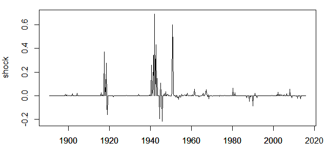
Figure 1: Military news shock (proportion of GDP) from Ramey and Zubairy (2018)

5.3 MGARCH model

While VAR uses historical data to predict the means, MGARCH forecasts future volatility.

Example 3: MGARCH model. Suppose a stochastic vector process ${\mathbf{y}}_{t}\in\mathbb{R}^{d_{y}}$ with $\mathbb{E}({\mathbf{y}}_{t})={\bf 0}$ follows Engle and Kroner (1995)’s MGARCH-BEKK(1,1) model

$${\mathbf{y}}_{t}={\mathbf{H}}_{t}^{1/2}\boldsymbol{\varepsilon}_{t}\,,~~\text{where}~~\boldsymbol{\varepsilon}_{t}\overset{{\rm i.i.d.}}{\sim}N({\mathbf{0}},{\mathbf{I}}_{d_{y}})\,,~~\text{and}~~{\mathbf{H}}_{t}={\mathbf{C}}^{{\mathrm{\scriptscriptstyle\top}}}{\mathbf{C}}+{\mathbf{D}}{\mathbf{y}}_{t-1}{\mathbf{y}}_{t-1}^{{\mathrm{\scriptscriptstyle\top}}}{\mathbf{D}}^{{\mathrm{\scriptscriptstyle\top}}}+{\mathbf{B}}{\mathbf{H}}_{t-1}{\mathbf{B}}^{{\mathrm{\scriptscriptstyle\top}}}\,,$$ (21)

where ${\mathbf{D}}$ and ${\mathbf{B}}$ are $d_{y}\times d_{y}$ parameter matrices, ${\mathbf{C}}$ is a $d_{y}\times d_{y}$ triangular matrix. Denote $\mathcal{J}_{-\infty}^{t}$ as the $\sigma$-filed generated by $\{{\mathbf{y}}_{s}\}$ up to and including time $t$. Then by (21), we have $\mathbb{E}({\mathbf{y}}_{t}{\mathbf{y}}_{t}^{{\mathrm{\scriptscriptstyle\top}}}|\,\mathcal{J}_{-\infty}^{t-2})={\mathbf{C}}^{{\mathrm{\scriptscriptstyle\top}}}{\mathbf{C}}+{\mathbf{D}}\mathbb{E}({\mathbf{y}}_{t-1}{\mathbf{y}}_{t-1}^{{\mathrm{\scriptscriptstyle\top}}}|\,\mathcal{J}_{-\infty}^{t-2}){\mathbf{D}}^{{\mathrm{\scriptscriptstyle\top}}}+{\mathbf{B}}\mathbb{E}({\mathbf{y}}_{t-1}{\mathbf{y}}_{t-1}^{{\mathrm{\scriptscriptstyle\top}}}|\,\mathcal{J}_{-\infty}^{t-2}){\mathbf{B}}^{{\mathrm{\scriptscriptstyle\top}}}$, which implies

$$\mathbb{E}({\mathbf{y}}_{t}{\mathbf{y}}_{t}^{{\mathrm{\scriptscriptstyle\top}}}-{\mathbf{C}}^{{\mathrm{\scriptscriptstyle\top}}}{\mathbf{C}}-{\mathbf{D}}{\mathbf{y}}_{t-1}{\mathbf{y}}_{t-1}^{{\mathrm{\scriptscriptstyle\top}}}{\mathbf{D}}^{{\mathrm{\scriptscriptstyle\top}}}-{\mathbf{B}}{\mathbf{y}}_{t-1}{\mathbf{y}}_{t-1}^{{\mathrm{\scriptscriptstyle\top}}}{\mathbf{B}}^{{\mathrm{\scriptscriptstyle\top}}}|\,\mathcal{J}_{-\infty}^{t-2})={\bf 0}\,.$$ (22)

Let ${\mathbf{q}}^{K}({\mathbf{y}}_{t-2})=\{q^{K}_{1}({\mathbf{y}}_{t-2}),\ldots,q^{K}_{K}({\mathbf{y}}_{t-2})\}^{{\mathrm{\scriptscriptstyle\top}}}$ denote a $K\times 1$ vector of known basis functions which, as $K\to\infty$, well approximate square integrable functions of ${\mathbf{y}}_{t-2}$, such as polynomial splines, B-splines, and power series. Then the conditional moment restrictions in (22) lead to a large number of unconditional moments

$$\mathbb{E}\{{\mathbf{g}}_{1}({\mathbf{x}}_{t};\boldsymbol{\theta}_{0})\}:=\mathbb{E}\{{\rm vech}({\mathbf{y}}_{t}{\mathbf{y}}_{t}^{{\mathrm{\scriptscriptstyle\top}}}-{\mathbf{C}}^{{\mathrm{\scriptscriptstyle\top}}}{\mathbf{C}}-{\mathbf{D}}{\mathbf{y}}_{t-1}{\mathbf{y}}_{t-1}^{{\mathrm{\scriptscriptstyle\top}}}{\mathbf{D}}^{{\mathrm{\scriptscriptstyle\top}}}-{\mathbf{B}}{\mathbf{y}}_{t-1}{\mathbf{y}}_{t-1}^{{\mathrm{\scriptscriptstyle\top}}}{\mathbf{B}}^{{\mathrm{\scriptscriptstyle\top}}})\otimes{\mathbf{q}}^{K}({\mathbf{y}}_{t-2})\}={\bf 0}\,,$$ (23)

where ${\mathbf{x}}_{t}=({\mathbf{y}}_{t}^{{\mathrm{\scriptscriptstyle\top}}},{\mathbf{y}}_{t-1}^{{\mathrm{\scriptscriptstyle\top}}},{\mathbf{y}}_{t-2}^{{\mathrm{\scriptscriptstyle\top}}})^{{\mathrm{\scriptscriptstyle\top}}}$ and $\boldsymbol{\theta}_{0}=\{{\rm vech}({\mathbf{C}})^{{\mathrm{\scriptscriptstyle\top}}},{\rm vec}({\mathbf{D}})^{{\mathrm{\scriptscriptstyle\top}}},{\rm vec}({\mathbf{B}})^{{\mathrm{\scriptscriptstyle\top}}}\}^{{\mathrm{\scriptscriptstyle\top}}}$. Moreover, (21) also implies

$$\mathbb{E}\{{\mathbf{g}}_{2}({\mathbf{x}}_{t};\boldsymbol{\theta}_{0})\}:=\mathbb{E}\{({\mathbf{y}}_{t}{\mathbf{y}}_{t}^{{\mathrm{\scriptscriptstyle\top}}}-{\mathbf{C}}^{{\mathrm{\scriptscriptstyle\top}}}{\mathbf{C}}-{\mathbf{D}}{\mathbf{y}}_{t-1}{\mathbf{y}}_{t-1}^{{\mathrm{\scriptscriptstyle\top}}}{\mathbf{D}}^{{\mathrm{\scriptscriptstyle\top}}}){\mathbf{y}}_{t-1}\}={\bf 0}\,.$$

Together, they produce the moment constraints ${\mathbf{g}}({\mathbf{x}}_{t};\boldsymbol{\theta}_{0})=\{{\mathbf{g}}_{1}({\mathbf{x}}_{t};\boldsymbol{\theta}_{0})^{{\mathrm{\scriptscriptstyle\top}}},{\mathbf{g}}_{2}({\mathbf{x}}_{t};\boldsymbol{\theta}_{0})^{{\mathrm{\scriptscriptstyle\top}}}\}^{{\mathrm{\scriptscriptstyle\top}}}$.

Figure 2: The parameter matrix ${\mathbf{D}}$ in the MGARCH model. Left: $d_{y}=10$, right: $d_{y}=30$

Table 4: The performance of the PEL estimator in the MGARCH model

		Case I			Case II
$(n,d_{y})$	Method	MSE	Bias2	Var	MSE	Bias2	Var
(50,10)	PEL	0.139	0.003	0.136	0.141	0.004	0.137
	MLE	×	×	×	×	×	×
	$\ell_{1}$-MLE	×	×	×	×	×	×
(80,10)	PEL	0.060	0.025	0.035	0.060	0.025	0.035
	MLE	×	×	×	×	×	×
	$\ell_{1}$-MLE	×	×	×	×	×	×
(50,30)	PEL	0.125	0.005	0.119	0.130	0.005	0.125
	MLE	×	×	×	×	×	×
	$\ell_{1}$-MLE	×	×	×	×	×	×
(80,30)	PEL	0.050	0.008	0.043	0.050	0.008	0.043
	MLE	×	×	×	×	×	×
	$\ell_{1}$-MLE	×	×	×	×	×	×

Note: Marked by “×”, MLE and $\ell_{1}$-MLE fail to converge numerically.

Table 5: Coverage frequency and median length of PPEL-based CIs in the MGARCH model

	Coverage frequency						Median CI length
	Case I			Case II			Case I			Case II
$(n,d_{y})$	90%	95%	99%	90%	95%	99%	90%	95%	99%	90%	95%	99%
(50, 10)	0.830	0.902	0.978	0.882	0.922	0.960	2.634	3.138	4.124	4.692	5.591	7.347
(80, 10)	0.880	0.932	0.988	0.896	0.938	0.982	2.730	3.253	4.275	2.827	3.369	4.428
(50, 30)	0.874	0.934	0.985	0.878	0.929	0.976	2.520	3.003	3.947	2.457	2.928	3.848
(80, 30)	0.917	0.937	0.973	0.914	0.943	0.971	2.133	2.541	3.340	2.215	2.639	3.468

We experiment with MGARCH in (21) under the following parameter matrices ${\mathbf{C}},{\mathbf{D}},{\mathbf{B}}$:

• Case I (Diagonal): ${\mathbf{C}}={\mathbf{I}}_{d_{y}}$, ${\mathbf{B}}=0.6{\mathbf{I}}_{d_{y}}$, and ${\mathbf{D}}=0.6{\mathbf{I}}_{d_{y}}$.

• Case II (Sparse): ${\mathbf{C}}={\mathbf{I}}_{d_{y}}$, ${\mathbf{B}}=0.6{\mathbf{I}}_{d_{y}}$, and ${\mathbf{D}}$ is a general sparse matrix with nonzero elements of the value $0.6$ on the diagonal and $0.1$ off the diagonal, as shown in Figure 2.

In our estimation, we specifically choose ${\mathbf{q}}^{K}({\mathbf{y}}_{t-2})=(y_{t-2,1},\ldots,y_{t-2,5})^{{\mathrm{\scriptscriptstyle\top}}}$ in (23). For convenience in the simulation, we randomly choose a point near $\boldsymbol{\theta}_{0}$ as the initial value, $\boldsymbol{\theta}^{0}=\boldsymbol{\theta}_{0}+\boldsymbol{\varepsilon}$ where $\boldsymbol{\varepsilon}\sim N({\mathbf{0}},0.5^{2}{\mathbf{I}}_{p})$, for all three estimators: PEL, MLE and $\ell_{1}$-penalized MLE ($\ell_{1}$-MLE). Table 4 summarizes the performances of the estimators. MLE and $\ell_{1}$-MLE fail to numerically converge in all settings — in our experiments, MLE and $\ell_{1}$-MLE numerically break down even if the initial value is set as the true $\boldsymbol{\theta}_{0}$, for the dimension of the parameter here surpasses the capacity of these two methods. In sharp contrast, PEL maintains robustness. The MSE of PEL decreases as $d_{y}$ gets bigger under the same $n$, because the significantly higher parameter dimension $p=2d_{y}^{2}+d_{y}(d_{y}+1)/2$ of MGARCH enhances relative sparsity and thereby the effectiveness of the penalization. Moreover, Table 5 shows that PPEL’s coverage frequency aligns well with the nominal ones.

6 Empirical applications

Given the reasonable performance of our PEL/PPEL procedure in the simulations, we apply this method to three real-data economic and financial applications.

6.1 Sectoral inflation

Inflation is a key macroeconomic indicator which serves as a signal of broad economic conditions, helping policymakers, businesses, and households make informed decisions. Controlling inflation, as one of the Federal Reserve’s dual mandates, is vital for maintaining economic stability and overall well-being. Inflation is measured by the growth rate of a price index. Besides the consumer price index (CPI), the personal consumption expenditures (PCE) price index is the Fed’s primary measure for monetary policies. PCE has a wide coverage, with its sectoral indices breaking down overall price changes into sectors such as food, housing, energy, healthcare, and so on. Examining how prices evolve and co-move across sectors helps pinpoint the source of inflation.

Following the onset of the COVID-19 pandemic, the United States has seen considerable variations in its inflation rate. Notably, in December 2021, inflation peaked at 7.0%, marking the highest level in several decades, driven by surging demand and disruptions in the supply chain. This prompted the Federal Reserve to implement stricter monetary policies. By late 2023, the inflation rate had decreased to approximately 3.0%. The data utilized for this empirical analysis is sourced directly from the Bureau of Economic Analysis, which publishes the PCE. It includes quarter-to-quarter changes in 16 sectoral PCE indices that are seasonally adjusted, covering the period from the first quarter of 1959 to the third quarter of 2023 (259 quarters).

To understand the dynamics and sectoral spillover effects, we follow the implementation of our simulation in Section 5.1 to fit a 16-sector VAR(1). The estimate of coefficient matrix is shown in Figure 3. While some sectors have upstream-downstream relationships, other sectors are less connected. One salient feature is that most autoregressive coefficients (those on the diagonal) are non-zeros, which is a key driving force of the persistence of inflation. Secondly, the estimated matrix is overall quite sparse. Notice that V7: Gasoline and other energy goods is much more volatile than other sectors, due to weather conditions, geopolitical uncertainty, and occasional energy crises, and therefore the fitting mechanism delivers many more active coefficients along its row to reduce the magnitude of the corresponding residual.

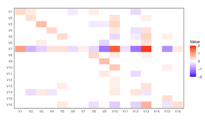
Figure 3: The AR(1) coefficient matrix of the 16-sector VAR(1) model

Notes: List of the code and name of each sector.

V1: Motor vehicles and parts, V2: Furnishings and durable household equipment,

V3: Recreational goods and vehicles, V4: Other durable goods, V5: Food and beverages purchased for off-premises consumption, V6: Clothing and footwear, V7: Gasoline and other energy goods, V8: Other nondurable goods, V9: Housing and utilities, V10: Health care,

V11: Transportation services, V12: Recreation services, V13: Food services and accommodations, V14: Financial services and insurance, V15: Other services, V16: Final consumption expenditures of nonprofit institutions serving households (NPISHs).

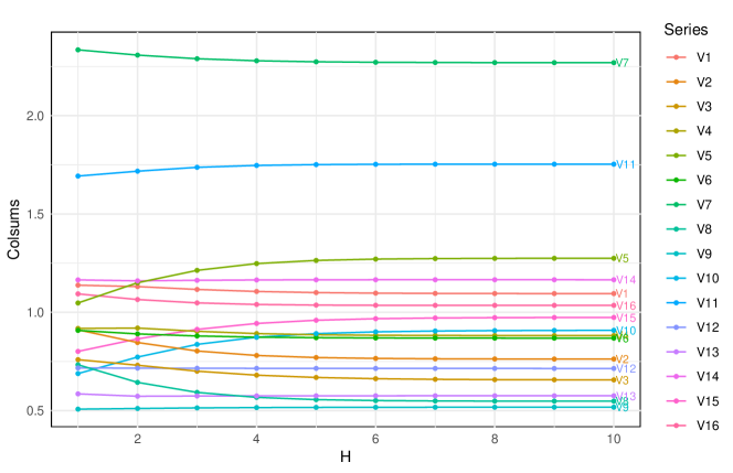
Figure 4: Directional connectedness: The colsums of $\widetilde{\mathbf{D}}^{g,h}$ for $h=1,\ldots,10$

We further follow Diebold and Yılmaz (2014)’s decomposition to measure the relative weight of the shocks. The $h$-step generalized variance decomposition matrix ${\mathbf{D}}^{g,h}=(d_{i,j}^{{g,h}})$ is

$$d_{i,j}^{g,h}=\frac{\sigma_{\varepsilon,j,j}^{-1}\sum_{\ell=0}^{h-1}(\boldsymbol{\iota}_{i}^{{\mathrm{\scriptscriptstyle\top}}}{\mathbf{G}}_{1}^{\ell}\boldsymbol{\Sigma}_{\varepsilon}\boldsymbol{\iota}_{j})^{2}}{\sum_{\ell=0}^{h-1}\boldsymbol{\iota}_{i}^{{\mathrm{\scriptscriptstyle\top}}}{\mathbf{G}}_{1}^{\ell}\boldsymbol{\Sigma}_{\varepsilon}{\mathbf{G}}_{1}^{\ell,{\mathrm{\scriptscriptstyle\top}}}\boldsymbol{\iota}_{i}}\,,$$

where $\boldsymbol{\Sigma}_{\varepsilon}$ is the covariance matrix of the disturbance vector, $\sigma_{\varepsilon,j,j}$ is the $j$-th diagonal element of $\boldsymbol{\Sigma}_{\varepsilon}$, and $\boldsymbol{\iota}_{i}$ is the selection vector with one as the $i$-th element and zeros otherwise. We normalize each entry of the generalized variance decomposition matrix ${\mathbf{D}}^{g,h}$ by the row sum, denoted by $\widetilde{\mathbf{D}}^{g,h}$, and then calculate the column sums to measure the out-variance of each sector for different horizons $h$. The results are shown in Figure 4. Each dot represents the relative fraction source of the variation that is originated from a particular sector over $h=1,\ldots,10$. The two major sources of variation come from V7:Gasoline and other energy goods and V11:Transportation services. The former exhibits the highest variance among all sectors, as mentioned above, and the latter is tightly linked to the energy sector. They spread out the variations to other sectors via the interconnection of the network. This example illustrates that our PEL method allows us to work with the granular sectoral level indices to inspect the relative importance and dynamics, which is much richer than simply looking at an overall univariate inflation measure at the national level.

6.2 Government spending multipliers

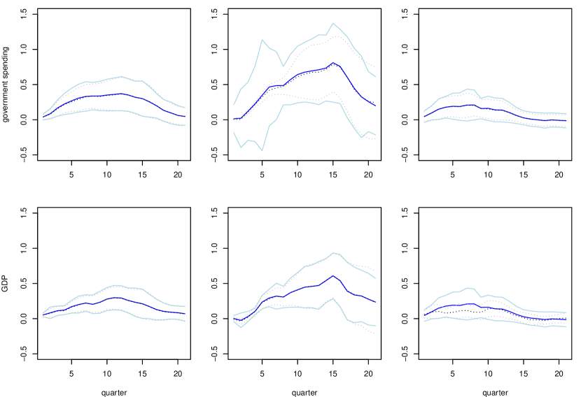
Figure 5: Point estimates of IRF and 95% confidence intervals computed from LP (gray dotted line) and PPEL (blue solid line). The first column: the full sample; the second column: subsample of high-unemployment state; the third column: subsample of low-unemployment state

John Maynard Keynes introduced the government spending multiplier in his General Theory, which is foundational to his broader theories on fiscal policy and its role in managing economic activities, especially during recessions. Despite the importance of the concept, the measurement of the multiplier is by no means straightforward, because it is difficult to isolate it from confounding factors. An influential recent empirical study of the fiscal multiplier by Ramey and Zubairy (2018) uses quarterly data from 1889 to 2015. We follow the same specification to replicate their Figure 5, and then use our method to re-evaluate the IRFs. While our simulation in Section 5.2 utilizes only the real data of news shock shown in Figure 1, here in the empirical application we use the real time series of government spending and GDP. The LP specification in (20) sets either government spending or GDP as the target variable, and $\text{shock}_{t}$ is again the military spending news. The control variable ${\mathbf{w}}_{t-1}$ includes four lags of the news shock, government spending, and GDP. A state-dependent alternative version of the model (20) is also considered for the subsamples of high/low-unemployment states, respectively.

The empirical results are reported in Figure 5. It consists of six subplots, each being the IRF of the fiscal multiplier of the news shock to government spending (the first row) and GDP (the second row). The three columns represent the full sample (the first column), the high unemployment periods (the second column, 181 observations), and the low-unemployment periods (the third column, 320 observations), following the original empirical study. The split of “bad times” and “good times” is to check the structural stability of the IRFs under distinctive states of the economy.

The two methods, Ramey and Zubairy (2018)’s LP estimated by OLS (which is the same as the original paper) and this paper’s PPEL, return very close point estimates. The main message is that the fiscal multipliers are mostly much smaller than unity in American history through booms and recessions, so that counter-cyclical policies likely have dampened effects. However, there are visually salient gaps in terms of the interval estimates. Recall that our simulation in Section 5.2 has shown that, despite the narrower length of CI, the coverage of LP may deviate from the nominal coverage frequency. It is echoed by Figure 5 where PPEL has slightly wider CIs than LP for obtaining nominal CIs. In particular, in the second column of the subplots, the LP with a small $h=0,1,\ldots,5$ has extremely narrow confidence intervals; given a sample size of 181 observations, it is surprising to see that the confidence intervals are even much narrower than those from the full sample of 501 as in the first column. The counterintuitive observation is likely the consequence of the low empirical coverage probability that deviates from the designated nominal coverage rate. On the other hand, the length of the confidence intervals from PPEL suitably reflects the statistical randomness that corresponds to the sample sizes. The evidence suggests that the latter provides more reasonable quantification of the underlying uncertainty.

6.3 Volatility spillover across banks

In the last empirical application, we explore the volatility spillover effect of 16 stocks from China’s banking industry, with data from the CSMAR database (https://data.csmar.com/). We investigate the daily log-returns of these stocks from January 2, 2024, to April 19, 2024. Table 6 summarizes the descriptive statistics of the time series and their pairwise sample correlation. The sample means of all stocks are very close to 0, and the sample kurtosises of several stocks are much larger than 3. Moreover, all pairwise sample correlations are positive. These findings motivate us to employ the MGARCH-BEKK(1,1) model specified in (21) to study the interconnection of volatility.

Table 6: Summary of 16 stocks

	PA	NB	PF	HX	MS	ZS	NJ	XY	BJ	NY	JT	GS	GD	JS	ZG	ZX
mean	0.00	0.00	0.00	0.00	0.00	0.00	0.00	0.00	0.00	0.00	0.00	0.00	0.00	0.00	0.00	0.00
sd	0.02	0.02	0.01	0.01	0.01	0.01	0.01	0.01	0.01	0.01	0.01	0.01	0.01	0.01	0.01	0.02
skew	2.32	1.01	0.09	-0.06	0.45	1.06	-0.06	-3.20	-0.34	-0.52	-0.18	-0.76	-2.30	-0.41	0.21	0.58
kurtosis	10.32	1.75	0.32	1.04	0.49	1.96	0.63	17.43	0.45	0.07	1.31	1.14	11.79	1.36	1.14	4.40
PA		0.64	0.69	0.47	0.50	0.77	0.46	0.54	0.43	0.27	0.37	0.34	0.50	0.31	0.28	0.50
NB			0.56	0.46	0.45	0.65	0.42	0.41	0.34	0.24	0.39	0.29	0.37	0.33	0.31	0.50
PF				0.71	0.68	0.71	0.65	0.50	0.57	0.55	0.65	0.59	0.52	0.62	0.62	0.47
HX					0.70	0.43	0.61	0.22	0.73	0.69	0.77	0.70	0.55	0.73	0.69	0.54
MS						0.41	0.59	0.31	0.58	0.56	0.57	0.57	0.57	0.60	0.58	0.52
ZS							0.34	0.54	0.33	0.30	0.44	0.37	0.44	0.34	0.36	0.47
NJ								0.30	0.78	0.56	0.63	0.66	0.55	0.67	0.63	0.46
XY									0.28	0.22	0.27	0.30	0.41	0.23	0.27	0.34
BJ										0.61	0.67	0.71	0.63	0.69	0.64	0.52
NY											0.89	0.92	0.61	0.89	0.88	0.40
JT												0.87	0.66	0.88	0.89	0.51
GS													0.64	0.88	0.87	0.47
GD														0.60	0.59	0.57
JS															0.91	0.45
ZG																0.43

Note: The full names of the abbreviations PA, NB, …, and ZX are listed in Table 7.

Recall that in the simulation in Section 5.3 a disturbed true value was used as an initial value for PEL. Here for real data, we follow Yao et al. (2024) to obtain an initial value. Specifically, we set the initial values for diagonal elements of ${\mathbf{C}},{\mathbf{D}}$ and ${\mathbf{B}}$ as square roots of estimated parameters of fitting each component series into a univariate GARCH(1,1) model, and the off-diagonal elements as random values sampled from $N(0,0.5^{2})$. Figure 6 plots the estimated structure of $\widehat{\mathbf{D}}$ and $\widehat{\mathbf{B}}$. Each arrow corresponds to a nonzero estimated off-diagonal element of $\widehat{\mathbf{D}}$ or $\widehat{\mathbf{B}}$. Specifically, if $\widehat{\mathbf{D}}$’s $(i,j)$-th element $\hat{d}_{i,j}\neq 0$, the directional line shoots from $i$ to $j$.

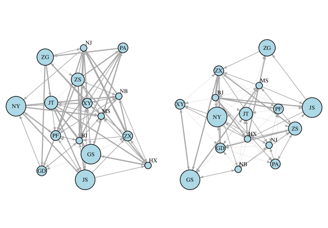
Figure 6: The network structures of estimated matrices $\widehat{\mathbf{D}}$ (left) and $\widehat{\mathbf{B}}$ (right). The thickness of an edge represents the relative magnitude of a coefficient, and the relative size of a vertex embodies the market value of a bank

To check the estimated patterns of connection, we further compute the numbers of outgoing links, incoming links, and net links of the estimated $\widehat{\mathbf{D}}$ graph, as suggested by Dhaene et al. (2022). Table 7 shows that the major national banks are the sources of shocks. They include the four biggest ones (Industrial and Commercial Bank of China (GS), Agricultural Bank of China (NY), Bank of China (ZG), China Construction Bank (JS)), as well as Ping An Bank (PA), China Merchants Bank (ZS), and China CITIC Bank (ZX). These banks are central to China’s financial system and play a significant role in sustaining the country’s economic growth. On the other hand, several joint-stock commercial banks rank as top destinations of shocks. They mostly feature a higher level of market orientation and substantial exposure to market forces. These characteristics contribute to heightened sensitivity to market shocks and greater interconnectedness, resulting in more significant volatility spillover. The large national banks are the main focus in hedging the risk of China’s banking industry. Our empirical exercise quantifies the volatility spillover effects, which can be of interest for both practitioners of risk management and policymakers.

Table 7: Rank of 16 stocks in terms of net spillover links

Ticker	Company	Out	In	Out-In	Ticker	Company	Out	In	Out-In
GS	Industrial and Commercial Bank of China	9	4	5	JS	China Construction Bank	5	4	1
ZG	Bank of China	6	2	4	HX	Huaxia Bank	4	5	-1
PA	Ping An Bank	5	2	3	NJ	Bank of Nanjing	5	6	-1
NY	Agricultural Bank of China	5	3	2	GD	China Everbright Bank	3	4	-1
ZX	China CITIC Bank	6	4	2	BJ	Bank of Beijing	6	9	-3
NB	Ningbo Bank	7	6	1	XY	Industrial Bank	5	9	-4
ZS	China Merchants Bank	7	6	1	PF	Shanghai Pudong Development Bank	5	10	-5
JT	Bank of Communications	6	5	1	MS	China Minsheng Bank	3	8	-5

7 Conclusion

This study investigates the PEL method in the analysis of multivariate time series models characterized by high-dimensional moments and parameters. These models are prevalent in the fields of economics and finance, as seen in VAR, local projection, and volatility models. We develop the marginal EL and demonstrate the consistency of PEL. Additionally, we introduce PPEL for the inference of low-dimensional parameters, which effectively removes the impact of nuisance parameters and maintains asymptotic normality centered at zero. Comprehensive Monte Carlo simulations provide evidence for the validity of our approach. We illustrate its practical application in three empirical examples using real data: the dynamics of the USA’s inflation, the IRF of news shocks to government spending and GDP, and the stock price volatility spillovers among Chinese banks.

The PEL/PPEL method provides a flexible and adaptable strategy. It serves as a promising technique for regulating the high dimensionality in parameters and moments. This approach can be extended in various directions. For example, though this paper does not address time series models with endogeneity due to space constraints, instruments can be easily integrated into our framework using moment conditions.

Appendix Appendix A The main proofs

In the sequel, we use $C$ to denote a generic finite positive constant that may be different in different uses. For any given index set $\mathcal{L}\subset[r]$ and $\boldsymbol{\theta}\in\boldsymbol{\Theta}$, we write $\widehat{\boldsymbol{\Gamma}}_{{\mathcal{\scriptscriptstyle L}}}(\boldsymbol{\theta})=\nabla_{\boldsymbol{\theta}_{{\mathcal{\scriptscriptstyle S}}}}\bar{{\mathbf{g}}}_{{\mathcal{\scriptscriptstyle L}}}(\boldsymbol{\theta})$ and $\widehat{\boldsymbol{\Gamma}}(\boldsymbol{\theta})=\widehat{\boldsymbol{\Gamma}}_{[r]}(\boldsymbol{\theta})$ for simplicity. For any $\boldsymbol{\theta}\in\boldsymbol{\Theta}$ and $\boldsymbol{\lambda}\in\hat{\Lambda}_{n}(\boldsymbol{\theta})$, we define

$$f(\boldsymbol{\lambda};\boldsymbol{\theta}) =\frac{1}{n}\sum_{t=1}^{n}\log\{1+\boldsymbol{\lambda}^{{\mathrm{\scriptscriptstyle\top}}}{{\mathbf{g}}_{t}(\boldsymbol{\theta})}\}-\sum_{j=1}^{r}P_{2,\nu}(|\lambda_{j}|)\,,$$

$$S_{n}(\boldsymbol{\theta}) =\max_{\boldsymbol{\lambda}\in\hat{\Lambda}_{n}(\boldsymbol{\theta})}f(\boldsymbol{\lambda};\boldsymbol{\theta})+\sum_{k=1}^{p}P_{1,\pi}(|\theta_{k}|)\,,$$

and $\hat{\boldsymbol{\lambda}}(\boldsymbol{\theta})=\arg\max_{\boldsymbol{\lambda}\in\hat{\Lambda}_{n}(\boldsymbol{\theta})}f(\boldsymbol{\lambda};\boldsymbol{\theta})$. For some constant $c\in(C_{*},1)$ with $C_{*}$ specified in (9), define $\mathcal{M}_{\boldsymbol{\theta}}(c)=\{j\in[r]:|\bar{g}_{j}(\boldsymbol{\theta})|\geq c\nu\rho_{2}^{\prime}(0^{+})\}$ for $\boldsymbol{\theta}\in\boldsymbol{\Theta}$.

A.1 Proof of Theorem 1

Recall $\aleph_{n}=n^{-3\varphi/(6\varphi+2)}(\log r)^{1/2}$. To prove Theorem 1, we need Lemmas 1–4, whose proofs are given in Sections S1.1–S1.4 of the supplementary material, respectively.

Lemma 1.

Under Conditions 1, 3(a) and 3(b), it holds that $|\bar{{\mathbf{g}}}(\boldsymbol{\theta}_{0})|_{\infty}=O_{{\mathrm{p}}}(\aleph_{n})$ and

$$\max_{j_{1},j_{2}\in[r]}\bigg{|}\frac{1}{n}\sum_{t=1}^{n}\big{[}g_{t,j_{1}}(\boldsymbol{\theta}_{0})g_{t,j_{2}}(\boldsymbol{\theta}_{0})-\mathbb{E}\{g_{t,j_{1}}(\boldsymbol{\theta}_{0})g_{t,j_{2}}(\boldsymbol{\theta}_{0})\}\big{]}\bigg{|}=O_{{\mathrm{p}}}(\aleph_{n})$$

provided that $L_{n}^{\varphi}\log(rn)\ll n^{\varphi/(3\varphi+1)}$.

Lemma 2.

Let $\mathscr{T}=\{\mathcal{T}\subset[r]:|\mathcal{T}|\leq\ell_{n}\}$ and $\boldsymbol{\Theta}_{n}=\{\boldsymbol{\theta}=(\boldsymbol{\theta}_{\mathcal{\scriptscriptstyle S}}^{{\mathrm{\scriptscriptstyle\top}}},\boldsymbol{\theta}_{{\mathcal{\scriptscriptstyle S}}^{\rm c}}^{{\mathrm{\scriptscriptstyle\top}}})^{{\mathrm{\scriptscriptstyle\top}}}\in\boldsymbol{\Theta}:|\boldsymbol{\theta}_{{\mathcal{\scriptscriptstyle S}}}-\boldsymbol{\theta}_{0,{\mathcal{\scriptscriptstyle S}}}|_{\infty}\leq O_{{\mathrm{p}}}(b_{n}^{1/2}),|\boldsymbol{\theta}_{{\mathcal{\scriptscriptstyle S}}^{\rm c}}|_{1}\leq\aleph_{n}\}$. Under Conditions 1, 3 and 4(a), if $L_{n}^{\varphi}\log(rn)\ll n^{\varphi/(3\varphi+1)}$, $s^{2}\ell_{n}b_{n}=o(1)$ and $\ell_{n}\aleph_{n}=o(1)$, then

$$\sup_{\boldsymbol{\theta}\in\boldsymbol{\Theta}_{n}}\sup_{\mathcal{T}\in\mathscr{T}}\|\widehat{{\mathbf{V}}}_{\mathcal{\scriptscriptstyle T}}(\boldsymbol{\theta})-\mathbb{E}\{\widehat{{\mathbf{V}}}_{\mathcal{\scriptscriptstyle T}}(\boldsymbol{\theta}_{0})\}\|_{2}=O_{{\mathrm{p}}}(s\ell_{n}^{1/2}b_{n}^{1/2})+O_{{\mathrm{p}}}(\ell_{n}\aleph_{n})\,.$$

Recall $\mathcal{M}_{\boldsymbol{\theta}}^{*}=\{j\in[r]:|\bar{g}_{j}(\boldsymbol{\theta})|\geq C_{*}\nu\rho_{2}^{\prime}(0^{+})\}$ for some constant $C_{*}\in(0,1)$. Lemma 3 provides a general result for the property of the Lagrange multiplier $\hat{\boldsymbol{\lambda}}(\boldsymbol{\theta})$, and Lemma 4 specifies the property of $\hat{\boldsymbol{\lambda}}(\boldsymbol{\theta}_{0})$.

Lemma 3.

Let $\{\boldsymbol{\theta}_{n}\}$ be a sequence in $\boldsymbol{\Theta}$ and $P_{2,\nu}(\cdot)\in\mathcal{P}$ be a convex function with bounded second-order derivatives around $0$, where $\mathcal{P}$ is defined in (5). For some constant $c\in(C_{*},1)$, assume that all the eigenvalues of $\widehat{{\mathbf{V}}}_{{\mathcal{\scriptscriptstyle M}}_{\boldsymbol{\theta}_{n}}(c)}(\boldsymbol{\theta}_{n})$ are uniformly bounded away from zero and infinity w.p.a.1. Let $|\bar{{\mathbf{g}}}_{{\mathcal{\scriptscriptstyle M}}_{{\boldsymbol{\theta}}_{n}}(c)}({\boldsymbol{\theta}}_{n})-\nu\rho_{2}^{\prime}(0^{+})$sgn$\{\bar{{\mathbf{g}}}_{{\mathcal{\scriptscriptstyle M}}_{{\boldsymbol{\theta}}_{n}}(c)}({\boldsymbol{\theta}}_{n})\}|_{2}=O_{{\mathrm{p}}}(u_{n})$ for some $u_{n}\to 0$. Assume there exists some non-random sequence $\{m_{n}\}$ such that $\mathbb{P}(|\mathcal{M}_{\boldsymbol{\theta}_{n}}^{*}|\leq m_{n})\to 1$ as $n\to\infty$. If $\max_{j\in[r]}\mathbb{E}_{n}\{|g_{t,j}(\boldsymbol{\theta}_{n})|^{\gamma}\}=O_{{\mathrm{p}}}(1)$ and $m_{n}^{1/2}u_{n}\ll\min\{\nu,n^{-1/\gamma}\}$, then w.p.a.1 there is a sparse global maxmizer $\hat{\boldsymbol{\lambda}}(\boldsymbol{\theta}_{n})$ for $f(\boldsymbol{\lambda};\boldsymbol{\theta}_{n})$ satisfying the three results: $\rm{(i)}$ $|\hat{\boldsymbol{\lambda}}(\boldsymbol{\theta}_{n})|_{2}=O_{{\mathrm{p}}}(u_{n})$, $\rm{(ii)}$ ${\rm{supp}}\{\hat{\boldsymbol{\lambda}}({\boldsymbol{\theta}}_{n})\}\subset\mathcal{M}_{\boldsymbol{\theta}_{n}}(c)$, and $\rm{(iii)}$ ${\rm{sgn}}(\hat{\lambda}_{n,j})=$ ${\rm{sgn}}\{\bar{g}_{j}(\boldsymbol{\theta}_{n})\}$ for any $j\in\mathcal{M}_{\boldsymbol{\theta}_{n}}(c)$ with $\hat{\lambda}_{n,j}\neq 0$, where $\hat{\boldsymbol{\lambda}}(\boldsymbol{\theta}_{n})=(\hat{\lambda}_{n,1},\dots,\hat{\lambda}_{n,r})^{{\mathrm{\scriptscriptstyle\top}}}$.

Lemma 4.

Let $P_{2,\nu}(\cdot)$ be a convex function for $\mathcal{P}$ defined in $\eqref{penalty}$. Under Conditions 1 and 3, if $L_{n}^{\varphi}\log(rn)\ll n^{\varphi/(3\varphi+1)}$ and $\ell_{n}\aleph_{n}\ll\min\{n^{-1/\gamma},\nu\}$, then w.p.a.1 there exists a sparse global maximizer $\hat{\boldsymbol{\lambda}}(\boldsymbol{\theta}_{0})=(\hat{\lambda}_{0,1},\dots,\hat{\lambda}_{0,r})^{\mathrm{\scriptscriptstyle\top}}$ for $f(\boldsymbol{\lambda};\boldsymbol{\theta}_{0})$ satisfying ${\rm{supp}}\{\hat{\boldsymbol{\lambda}}(\boldsymbol{\theta}_{0})\}\subset\mathcal{M}_{\boldsymbol{\theta}_{0}}(c)$ for some constant $c\in(C_{*},1)$.

Now we begin to prove Theorem 1. Let $\mathcal{G}_{0}=\text{supp}\{\hat{\boldsymbol{\lambda}}(\boldsymbol{\theta}_{0})\}$. It holds that

$$\begin{split}\max_{\boldsymbol{\lambda}\in\hat{\Lambda}_{n}(\boldsymbol{\theta}_{0})}f(\boldsymbol{\lambda};\boldsymbol{\theta}_{0})&=\max_{\boldsymbol{\eta}\in\hat{\Lambda}_{n}^{\dagger}(\boldsymbol{\theta}_{0})}\bigg{[}\frac{1}{n}\sum_{t=1}^{n}\log\{1+\boldsymbol{\eta}^{{\mathrm{\scriptscriptstyle\top}}}{\mathbf{g}}_{t,{\mathcal{\scriptscriptstyle G}}_{0}}(\boldsymbol{\theta}_{0})\}-\sum_{j=1}^{|\mathcal{G}_{0}|}P_{2,\nu}(|\eta_{j}|)\bigg{]}\\ &\leq\max_{\boldsymbol{\eta}\in\hat{\Lambda}_{n}^{\dagger}(\boldsymbol{\theta}_{0})}\frac{1}{n}\sum_{t=1}^{n}\log\{1+\boldsymbol{\eta}^{{\mathrm{\scriptscriptstyle\top}}}{\mathbf{g}}_{t,{\mathcal{\scriptscriptstyle G}}_{0}}(\boldsymbol{\theta}_{0})\}\,,\end{split}$$

where $\hat{\Lambda}_{n}^{\dagger}(\boldsymbol{\theta}_{0})=\{\boldsymbol{\eta}\in\mathbb{R}^{|\mathcal{G}_{0}|}:\boldsymbol{\eta}^{{\mathrm{\scriptscriptstyle\top}}}{\mathbf{g}}_{t,{\mathcal{\scriptscriptstyle G}}_{0}}(\boldsymbol{\theta}_{0})\in\mathcal{V},t\in[n]\}$ for some open interval $\mathcal{V}$ containing zero. Define $A_{n}(\boldsymbol{\theta}_{0};\boldsymbol{\eta})=n^{-1}\sum_{t=1}^{n}\log\{1+\boldsymbol{\eta}^{{\mathrm{\scriptscriptstyle\top}}}{\mathbf{g}}_{t,{\mathcal{\scriptscriptstyle G}}_{0}}(\boldsymbol{\theta}_{0})\}$ for any $\boldsymbol{\eta}\in\hat{\Lambda}_{n}^{\dagger}(\boldsymbol{\theta}_{0})$. Let $\tilde{\boldsymbol{\eta}}=\arg\max_{\boldsymbol{\eta}\in\hat{\Lambda}_{n}^{\dagger}(\boldsymbol{\theta}_{0})}A_{n}(\boldsymbol{\theta}_{0};\boldsymbol{\eta})$. Due to $\ell_{n}\aleph_{n}\ll n^{-1/\gamma}$, we can select $\delta_{n}$ satisfying $\ell_{n}^{1/2}\aleph_{n}\ll\delta_{n}\ll\ell_{n}^{-1/2}n^{-1/\gamma}$. Let $\bar{\boldsymbol{\eta}}=\arg\max_{\boldsymbol{\eta}\in\Lambda_{n}}A_{n}(\boldsymbol{\theta}_{0};\boldsymbol{\eta})$ with $\Lambda_{n}=\{\boldsymbol{\eta}\in\mathbb{R}^{|\mathcal{G}_{0}|}:|\boldsymbol{\eta}|_{2}\leq\delta_{n}\}$. Lemma 4 ensures $|\mathcal{G}_{0}|\leq|\mathcal{M}_{\boldsymbol{\theta}_{0}}(c)|\leq\ell_{n}$ w.p.a.1. By Condition 3(a), $\max_{t\in[n]}|{\mathbf{g}}_{t,{\mathcal{\scriptscriptstyle G}}_{0}}(\boldsymbol{\theta}_{0})|_{2}=O_{{\mathrm{p}}}(\ell_{n}^{1/2}n^{1/\gamma})$, which implies $\sup_{t\in[n],\boldsymbol{\eta}\in\Lambda_{n}}|\boldsymbol{\eta}^{{\mathrm{\scriptscriptstyle\top}}}{\mathbf{g}}_{t,{\mathcal{\scriptscriptstyle G}}_{0}}(\boldsymbol{\theta}_{0})|=o_{{\mathrm{p}}}(1)$. By Condition 3(c) and (S1.2) in the supplementary material, if $L_{n}^{\varphi}\log(rn)\ll n^{\varphi/(3\varphi+1)}$ and $\ell_{n}\aleph_{n}=o(1)$, we know $\lambda_{\min}\{\widehat{{\mathbf{V}}}_{{\mathcal{\scriptscriptstyle G}}_{0}}(\boldsymbol{\theta}_{0})\}$ is uniformly bounded away from zero w.p.a.1. By Taylor expansion, it holds w.p.a.1 that

$$\begin{split}0=A_{n}(\boldsymbol{\theta}_{0};{\bf 0})\leq A_{n}(\boldsymbol{\theta}_{0};\bar{\boldsymbol{\eta}})&=\bar{\boldsymbol{\eta}}^{{\mathrm{\scriptscriptstyle\top}}}\bar{{\mathbf{g}}}_{{\mathcal{\scriptscriptstyle G}}_{0}}(\boldsymbol{\theta}_{0})-\frac{1}{2n}\sum_{t=1}^{n}\frac{\bar{\boldsymbol{\eta}}^{\mathrm{\scriptscriptstyle\top}}{{\mathbf{g}}}_{t,{\mathcal{\scriptscriptstyle G}}_{0}}(\boldsymbol{\theta}_{0})^{\otimes 2}\bar{\boldsymbol{\eta}}}{\{1+\bar{c}\bar{\boldsymbol{\eta}}^{{\mathrm{\scriptscriptstyle\top}}}{\mathbf{g}}_{t,{\mathcal{\scriptscriptstyle G}}_{0}}(\boldsymbol{\theta}_{0})\}^{2}}\\ &\leq|\bar{\boldsymbol{\eta}}|_{2}|\bar{{\mathbf{g}}}_{{\mathcal{\scriptscriptstyle G}}_{0}}(\boldsymbol{\theta}_{0})|_{2}-C|\bar{\boldsymbol{\eta}}|_{2}^{2}\{1+o_{{\mathrm{p}}}(1)\}\end{split}$$ (A.1)

for some $\bar{c}\in(0,1)$. By Lemma 1, we have $|\bar{{\mathbf{g}}}(\boldsymbol{\theta}_{0})|_{\infty}=O_{{\mathrm{p}}}(\aleph_{n})$ provided that $L_{n}^{\varphi}\log(rn)\ll n^{\varphi/(3\varphi+1)}$, which implies $|\bar{{\mathbf{g}}}_{{\mathcal{\scriptscriptstyle G}}_{0}}(\boldsymbol{\theta}_{0})|_{2}=O_{{\mathrm{p}}}(\ell_{n}^{1/2}\aleph_{n})$. By (A.1), we have $|\bar{\boldsymbol{\eta}}|_{2}=O_{{\mathrm{p}}}(\ell_{n}^{1/2}\aleph_{n})=o_{{\mathrm{p}}}(\delta_{n})$, which implies $\bar{\boldsymbol{\eta}}\in\text{int}(\Lambda_{n})$ w.p.a.1. Since $\Lambda_{n}\subset\hat{\Lambda}_{n}^{\dagger}(\boldsymbol{\theta}_{0})$ w.p.a.1, it holds that $\tilde{\boldsymbol{\eta}}=\bar{\boldsymbol{\eta}}$ w.p.a.1 by the concavity of $A_{n}(\boldsymbol{\theta}_{0};\boldsymbol{\eta})$ and the convexity of $\hat{\Lambda}_{n}^{\dagger}(\boldsymbol{\theta}_{0})$. Hence, by (A.1), we have $\max_{\boldsymbol{\eta}\in\hat{\Lambda}_{n}^{\dagger}(\boldsymbol{\theta}_{0})}A_{n}(\boldsymbol{\theta}_{0};\boldsymbol{\eta})=O_{{\mathrm{p}}}(\ell_{n}\aleph_{n}^{2})$, which implies $\max_{\boldsymbol{\lambda}\in\hat{\Lambda}_{n}(\boldsymbol{\theta}_{0})}f(\boldsymbol{\lambda};\boldsymbol{\theta}_{0})=O_{{\mathrm{p}}}(\ell_{n}\aleph_{n}^{2})$. Recall $a_{n}=\sum_{k=1}^{p}P_{1,\pi}(|\theta_{0,k}|)$, $b_{n}=\max\{a_{n},\nu^{2}\}$ and $S_{n}(\boldsymbol{\theta})=\max_{\boldsymbol{\lambda}\in\hat{\Lambda}_{n}(\boldsymbol{\theta})}f(\boldsymbol{\lambda};\boldsymbol{\theta})+\sum_{k=1}^{p}P_{1,\pi}(|\theta_{k}|)$ for any $\boldsymbol{\theta}=(\theta_{1},\dots,\theta_{p})^{\mathrm{\scriptscriptstyle\top}}$. Notice that $\hat{\boldsymbol{\theta}}_{n}=\arg\min_{\boldsymbol{\theta}\in\boldsymbol{\Theta}_{*}}S_{n}(\boldsymbol{\theta})$ with $\boldsymbol{\Theta}_{*}=\{\boldsymbol{\theta}=(\boldsymbol{\theta}_{\mathcal{\scriptscriptstyle S}}^{{\mathrm{\scriptscriptstyle\top}}},\boldsymbol{\theta}_{{\mathcal{\scriptscriptstyle S}}^{\rm c}}^{{\mathrm{\scriptscriptstyle\top}}})^{{\mathrm{\scriptscriptstyle\top}}}\in\boldsymbol{\Theta}:|\boldsymbol{\theta}_{{\mathcal{\scriptscriptstyle S}}}-\boldsymbol{\theta}_{0,{\mathcal{\scriptscriptstyle S}}}|_{\infty}\leq c_{*},|\boldsymbol{\theta}_{{\mathcal{\scriptscriptstyle S}}^{\rm c}}|_{1}\leq\aleph_{n}\}$ for some fixed constant $c_{*}>0$. As we have shown above, $S_{n}(\boldsymbol{\theta}_{0})=O_{{\mathrm{p}}}(\ell_{n}\aleph_{n}^{2})+a_{n}=O_{{\mathrm{p}}}(b_{n})$. Since $\boldsymbol{\theta}_{0}\in\boldsymbol{\Theta}_{*}$, then $S_{n}(\hat{\boldsymbol{\theta}}_{n})\leq S_{n}(\boldsymbol{\theta}_{0})=O_{{\mathrm{p}}}(b_{n})$. We will show that $\hat{\boldsymbol{\theta}}_{n}\in\text{int}(\boldsymbol{\Theta}_{*})$ w.p.a.1. Our proof takes two steps: (i) to show that for any $\epsilon_{n}\to\infty$ satisfying $b_{n}\epsilon_{n}^{2}n^{2/\gamma}=o(1)$, there exists a universal constant $K>0$ independent of $\boldsymbol{\theta}$ such that $\mathbb{P}\{S_{n}(\boldsymbol{\theta})>Kb_{n}\epsilon_{n}^{2}\}\to 1$ as $n\to\infty$ for any $\boldsymbol{\theta}=(\boldsymbol{\theta}_{\mathcal{\scriptscriptstyle S}}^{{\mathrm{\scriptscriptstyle\top}}},\boldsymbol{\theta}_{{\mathcal{\scriptscriptstyle S}}^{\rm c}}^{{\mathrm{\scriptscriptstyle\top}}})^{{\mathrm{\scriptscriptstyle\top}}}\in\boldsymbol{\Theta}_{*}$ satisfying $|\boldsymbol{\theta}_{{\mathcal{\scriptscriptstyle S}}}-\boldsymbol{\theta}_{0,{\mathcal{\scriptscriptstyle S}}}|_{\infty}>\epsilon_{n}b_{n}^{1/2}$, which leads to $|\hat{\boldsymbol{\theta}}_{n,{\mathcal{\scriptscriptstyle S}}}-\boldsymbol{\theta}_{0,{\mathcal{\scriptscriptstyle S}}}|_{\infty}=O_{{\mathrm{p}}}(b_{n}^{1/2})$, and (ii) to show that $\hat{\boldsymbol{\theta}}_{n,{\mathcal{\scriptscriptstyle S}}^{\rm c}}=\bf 0$ w.p.a.1.

A.1.1 Proof of (i)

For any $\boldsymbol{\theta}=(\boldsymbol{\theta}_{\mathcal{\scriptscriptstyle S}}^{{\mathrm{\scriptscriptstyle\top}}},\boldsymbol{\theta}_{{\mathcal{\scriptscriptstyle S}}^{\rm c}}^{{\mathrm{\scriptscriptstyle\top}}})^{{\mathrm{\scriptscriptstyle\top}}}\in\boldsymbol{\Theta}_{*}$ satisfying $|\boldsymbol{\theta}_{\mathcal{\scriptscriptstyle S}}-\boldsymbol{\theta}_{0,{\mathcal{\scriptscriptstyle S}}}|_{\infty}>\epsilon_{n}b_{n}^{1/2}$, write $\boldsymbol{\theta}^{*}=(\boldsymbol{\theta}_{{\mathcal{\scriptscriptstyle S}}}^{\mathrm{\scriptscriptstyle\top}},\bf 0^{\mathrm{\scriptscriptstyle\top}})^{\mathrm{\scriptscriptstyle\top}}$. Define ${\mu}_{t,j_{0}}=\mathbb{E}\{g_{t,j_{0}}(\boldsymbol{\theta})\}$, $\bar{\mu}_{j_{0}}=\mathbb{E}\{\bar{g}_{j_{0}}(\boldsymbol{\theta})\}$ and $\bar{\mu}_{j_{0}}^{*}=\mathbb{E}\{\bar{g}_{j_{0}}(\boldsymbol{\theta}^{*})\}$ with $j_{0}=\arg\max_{j\in[r]}|\mathbb{E}\{\bar{g}_{j}(\boldsymbol{\theta}^{*})\}|$. Select $\tilde{\boldsymbol{\lambda}}=\delta^{*}b_{n}^{1/2}\epsilon_{n}{\mathbf{e}}_{j_{0}}$, where $\delta^{*}>0$ is a constant to be determined later, and ${\mathbf{e}}_{j_{0}}$ is an $r$-dimensional vector with the $j_{0}$-th component being $1$ and other components being $0$. Without loss of generality, we assume $\bar{\mu}_{j_{0}}^{*}>0$. By Condition 3(a), $\max_{t\in[n]}|g_{t,j_{0}}(\boldsymbol{\theta})|=O_{{\mathrm{p}}}(n^{1/\gamma})$, which implies $\max_{t\in[n]}|\tilde{\boldsymbol{\lambda}}^{\mathrm{\scriptscriptstyle\top}}{\mathbf{g}}_{t}(\boldsymbol{\theta})|=O_{{\mathrm{p}}}(b_{n}^{1/2}\epsilon_{n}n^{1/\gamma})=o_{{\mathrm{p}}}(1).$ Then $\tilde{\boldsymbol{\lambda}}\in\hat{\Lambda}_{n}(\boldsymbol{\theta})$ w.p.a.1. Write $\boldsymbol{\theta}=(\theta_{1},\dots,\theta_{p})^{\mathrm{\scriptscriptstyle\top}}$ and $\tilde{\boldsymbol{\lambda}}=(\tilde{\lambda}_{1},\dots,\tilde{\lambda}_{r})^{\mathrm{\scriptscriptstyle\top}}.$ By Taylor expansion, it holds w.p.a.1 that

$$S_{n}(\boldsymbol{\theta})\geq ~\frac{1}{n}\sum_{t=1}^{n}\log\{1+\tilde{\boldsymbol{\lambda}}^{{\mathrm{\scriptscriptstyle\top}}}{\mathbf{g}}_{t}(\boldsymbol{\theta})\}-\sum_{j=1}^{r}P_{2,\nu}(|\tilde{\lambda}_{j}|)+\sum_{k=1}^{p}P_{1,\pi}(|\theta_{k}|)$$

$$\geq ~\frac{1}{n}\sum_{t=1}^{n}\tilde{\lambda}_{j_{0}}g_{t,j_{0}}(\boldsymbol{\theta})-\frac{1}{n}\sum_{t=1}^{n}\{\tilde{\lambda}_{j_{0}}g_{t,j_{0}}(\boldsymbol{\theta})\}^{2}-P_{2,\nu}(|\tilde{\lambda}_{j_{0}}|)$$

$$\geq ~\frac{1}{n}\sum_{t=1}^{n}\tilde{\lambda}_{j_{0}}g_{t,j_{0}}(\boldsymbol{\theta})-\frac{1}{n}\sum_{t=1}^{n}\{\tilde{\lambda}_{j_{0}}g_{t,j_{0}}(\boldsymbol{\theta})\}^{2}-C\nu\tilde{\lambda}_{j_{0}}\,,$$

which implies

$$\mathbb{P}\big{\{}S_{n}(\boldsymbol{\theta})\leq Kb_{n}\epsilon_{n}^{2}\big{\}} \leq\bigg{[}\frac{1}{n}\sum_{t=1}^{n}\tilde{\lambda}_{j_{0}}g_{t,j_{0}}(\boldsymbol{\theta})-\frac{1}{n}\sum_{t=1}^{n}\{\tilde{\lambda}_{j_{0}}g_{t,j_{0}}(\boldsymbol{\theta})\}^{2}-C\nu\tilde{\lambda}_{j_{0}}\leq Kb_{n}\epsilon_{n}^{2}\bigg{]}+o(1)$$

$$\leq\mathbb{P}\bigg{[}\frac{1}{n}\sum_{t=1}^{n}\{g_{t,j_{0}}(\boldsymbol{\theta})-\mu_{t,j_{0}}\}\leq b_{n}^{1/2}\epsilon_{n}\bigg{\{}\frac{K}{\delta^{*}}+\frac{\delta^{*}}{n}\sum_{t=1}^{n}g_{t,j_{0}}^{2}(\boldsymbol{\theta})\bigg{\}}+C\nu-\bar{\mu}_{j_{0}}\bigg{]}+o(1)\,.$$

Write $\mathring{g}_{t,j_{0}}(\boldsymbol{\theta})=g_{t,j_{0}}^{2}(\boldsymbol{\theta})-\mathbb{E}\{g_{t,j_{0}}^{2}(\boldsymbol{\theta})\}$. By Hölder inequality and Condition 3(a), we have $\mathbb{E}\{g_{t,j_{0}}^{4}(\boldsymbol{\theta})\}\leq[\mathbb{E}\{|g_{t,j_{0}}(\boldsymbol{\theta})|^{2\gamma}\}]^{2/\gamma}\leq K_{4}^{2/\gamma}$ for any $t\in[n]$. For any $t_{1}\neq t_{2}$, Davydov’s inequality and Condition 3(a) yield $|{\rm{Cov}}\{\mathring{g}_{t_{1},j_{0}}(\boldsymbol{\theta}),\mathring{g}_{t_{2},j_{0}}(\boldsymbol{\theta})\}|\lesssim\exp(-CL_{n}^{-\varphi}|t_{1}-t_{2}|^{\varphi})$. Then there exists a universal positive constant $L>K_{4}^{1/\gamma}$ independent of $\boldsymbol{\theta}$ such that

$$\mathbb{P}\bigg{\{}\frac{1}{n}\sum_{t=1}^{n}g_{t,j_{0}}^{2}(\boldsymbol{\theta})>L\bigg{\}}\leq ~\mathbb{P}\bigg{\{}\frac{1}{n}\sum_{t=1}^{n}\mathring{g}_{t,j_{0}}(\boldsymbol{\theta})>L-K_{4}^{1/\gamma}\bigg{\}}\leq(L-K_{4}^{1/\gamma})^{-2}\mathbb{E}\bigg{[}\bigg{\{}\frac{1}{n}\sum_{t=1}^{n}{\mathring{g}}_{t,j_{0}}(\boldsymbol{\theta})\bigg{\}}^{2}\bigg{]}$$

$$\lesssim ~\frac{1}{n^{2}}\sum_{t=1}^{n}\mathbb{E}\big{[}\{{\mathring{g}}_{t,j_{0}}(\boldsymbol{\theta})\}^{2}\big{]}+\frac{1}{n^{2}}\sum_{t_{2}=1}^{n}\sum_{t_{1}=t_{2}+1}^{n}|{\rm Cov}\{\mathring{g}_{t_{1},j_{0}}(\boldsymbol{\theta}),\mathring{g}_{t_{2},j_{0}}(\boldsymbol{\theta})\}|$$ (A.2)

$$\lesssim ~\frac{1}{n}+\frac{1}{n^{2}}\sum_{t_{2}=1}^{n}\sum_{t_{1}=t_{2}+1}^{n}\exp(-CL_{n}^{-\varphi}|t_{1}-t_{2}|^{\varphi})\lesssim\frac{L_{n}}{n}=o(1)\,,$$

where the second inequality follows from the Markov inequality. Thus, by selecting $\delta^{*}=(K/L)^{1/2}$ we have

$$\mathbb{P}\big{\{}S_{n}(\boldsymbol{\theta})\leq Kb_{n}\epsilon_{n}^{2}\big{\}}\leq\mathbb{P}\bigg{[}\frac{1}{n}\sum_{t=1}^{n}\{g_{t,j_{0}}(\boldsymbol{\theta})-\mu_{t,j_{0}}\}\leq 2b_{n}^{1/2}\epsilon_{n}(KL)^{1/2}+C\nu-\bar{\mu}_{j_{0}}\bigg{]}+o(1)\,.$$

By Condition 2, we have $\bar{\mu}_{j_{0}}^{*}\geq K_{3}\epsilon_{n}b_{n}^{1/2}/2$. Recall $\aleph_{n}=n^{-3\varphi/(6\varphi+2)}(\log r)^{1/2}$. By Condition 4(a),

$$|\bar{\mu}_{j_{0}}-\bar{\mu}_{j_{0}}^{*}|\leq\max_{t\in[n]}\max_{k\notin\mathcal{S}}\mathbb{E}\biggl{\{}\sup_{\boldsymbol{\theta}\in\boldsymbol{\Theta}}\bigg{|}\frac{\partial g_{t,j_{0}}(\boldsymbol{\theta})}{\partial\theta_{k}}\bigg{|}\biggr{\}}|\boldsymbol{\theta}_{{\mathcal{\scriptscriptstyle S}}^{\rm c}}|_{1}\leq K_{7}|\boldsymbol{\theta}_{{\mathcal{\scriptscriptstyle S}}^{\rm c}}|_{1}=O(\aleph_{n})=o(b_{n}^{1/2})\,.$$

Therefore, $\bar{\mu}_{j_{0}}\geq K_{3}\epsilon_{n}b_{n}^{1/2}/3$ for a sufficiently large $n$. For a sufficiently small $K$ independent of $\boldsymbol{\theta}$, we have $2b_{n}^{1/2}\epsilon_{n}(KL)^{1/2}+C\nu-\bar{\mu}_{j_{0}}\leq-c\bar{\mu}_{j_{0}}$, where $c\in(0,1)$ is a universal constant. Due to ${L}^{\varphi}_{n}\log{n}\ll{n}^{\varphi/(3\varphi+1)}$ and $\ell_{n}\aleph_{n}\ll b_{n}^{1/2}$, then $L_{n}n^{-1}\ll b_{n}$. Analogous to (A.1.1), it holds that

$$\mathbb{P}\bigg{[}\frac{1}{n}\sum_{t=1}^{n}\{g_{t,j_{0}}(\boldsymbol{\theta})-\mu_{t,j_{0}}\}\leq 2b_{n}^{1/2}\epsilon_{n}(KL)^{1/2}+C\nu-\bar{\mu}_{j_{0}}\bigg{]}$$

$$~~~~~~\leq\mathbb{P}\bigg{[}\bigg{|}\frac{1}{n}\sum_{t=1}^{n}\{g_{t,j_{0}}(\boldsymbol{\theta})-\mu_{t,j_{0}}\}\bigg{|}\geq c\bar{\mu}_{j_{0}}\bigg{]}\lesssim(\epsilon_{n}^{2}b_{n})^{-1}\mathbb{E}\bigg{(}\bigg{[}\frac{1}{n}\sum_{t=1}^{n}\{g_{t,j_{0}}(\boldsymbol{\theta})-\mu_{t,j_{0}}\}\bigg{]}^{2}\bigg{)}$$

$$~~~~~~\lesssim(\epsilon_{n}^{2}b_{n}L_{n}^{-1}n)^{-1}=o(1)\,.$$

Then $\mathbb{P}\{S_{n}(\boldsymbol{\theta})\leq Kb_{n}\epsilon_{n}^{2}\}\to 0$ as $n\to\infty$. Hence, $|\hat{\boldsymbol{\theta}}_{n,{\mathcal{\scriptscriptstyle S}}}-\boldsymbol{\theta}_{0,{\mathcal{\scriptscriptstyle S}}}|_{\infty}=O_{{\mathrm{p}}}(b_{n}^{1/2})$. $\hfill\Box$

A.1.2 Proof of (ii)

If $\hat{\boldsymbol{\theta}}_{n,{\mathcal{\scriptscriptstyle S}}^{\rm c}}\neq\bf 0$, we define $\hat{\boldsymbol{\theta}}_{n}^{*}=(\hat{\boldsymbol{\theta}}_{n,{\mathcal{\scriptscriptstyle S}}}^{\mathrm{\scriptscriptstyle\top}},\bf 0^{{\mathrm{\scriptscriptstyle\top}}})^{\mathrm{\scriptscriptstyle\top}}$ and will show $S_{n}(\hat{\boldsymbol{\theta}}_{n}^{*})<S_{n}(\hat{\boldsymbol{\theta}}_{n})$ w.p.a.1. This will contradict the definition of $\hat{\boldsymbol{\theta}}_{n}$. Thus we have $\hat{\boldsymbol{\theta}}_{n,{\mathcal{\scriptscriptstyle S}}^{\rm c}}=\bf 0$ w.p.a.1. Write $\hat{\boldsymbol{\theta}}_{n}=(\hat{\theta}_{n,1},\dots,\hat{\theta}_{n,p})^{\mathrm{\scriptscriptstyle\top}}$. Due to $b_{n}^{1/2}=o(\min_{k\in\mathcal{S}}|\theta_{0,k}|)$ and (7), it holds that

$$\max_{\boldsymbol{\lambda}\in\hat{\Lambda}_{n}(\hat{\boldsymbol{\theta}}_{n})}f(\boldsymbol{\lambda};\hat{\boldsymbol{\theta}}_{n})\leq ~\max_{\boldsymbol{\lambda}\in\hat{\Lambda}_{n}(\boldsymbol{\theta}_{0})}f(\boldsymbol{\lambda};\boldsymbol{\theta}_{0})+\sum_{k=1}^{p}P_{1,\pi}(|\theta_{0,k}|)-\sum_{k=1}^{p}P_{1,\pi}(|\hat{\theta}_{n,k}|)$$

$$\leq ~O_{{\mathrm{p}}}(\ell_{n}\aleph_{n}^{2})+\sum_{k=1}^{s}P_{1,\pi}^{{}^{\prime}}\{c_{k}|\hat{\theta}_{n,k}|+(1-c_{k})|\theta_{0,k}|\}|\hat{\theta}_{n,k}-\theta_{0,k}|$$

$$= ~O_{{\mathrm{p}}}(\ell_{n}\aleph_{n}^{2})$$

for some $c_{k}\in(0,1)$. Since $\ell_{n}\aleph_{n}\ll n^{-1/\gamma}$, then we pick a $\delta_{n}$ satisfying $\ell_{n}^{1/2}\aleph_{n}\ll\delta_{n}\ll\ell_{n}^{-1/2}n^{-1/\gamma}$. Define

$$\boldsymbol{\beta}_{{\mathcal{\scriptscriptstyle M}}_{\hat{\boldsymbol{\theta}}_{n}}(\tilde{c})}(\hat{\boldsymbol{\theta}}_{n}):=\bar{{\mathbf{g}}}_{{\mathcal{\scriptscriptstyle M}}_{\hat{\boldsymbol{\theta}}_{n}}(\tilde{c})}(\hat{\boldsymbol{\theta}}_{n})-\nu\rho^{\prime}_{2}(0^{+})\mbox{\rm sgn}\{\bar{{\mathbf{g}}}_{{\mathcal{\scriptscriptstyle M}}_{\hat{\boldsymbol{\theta}}_{n}}(\tilde{c})}(\hat{\boldsymbol{\theta}}_{n})\}$$

for $\tilde{c}\in(C_{*},1)$ specified in Condition 5(a). Select $\boldsymbol{\lambda}^{*}$ satisfying $\boldsymbol{\lambda}_{{\mathcal{\scriptscriptstyle M}}_{\hat{\boldsymbol{\theta}}_{n}}(\tilde{c})}^{*}=\delta_{n}\boldsymbol{\beta}_{{\mathcal{\scriptscriptstyle M}}_{\hat{\boldsymbol{\theta}}_{n}}(\tilde{c})}(\hat{\boldsymbol{\theta}}_{n})/|\boldsymbol{\beta}_{{\mathcal{\scriptscriptstyle M}}_{\hat{\boldsymbol{\theta}}_{n}}(\tilde{c})}(\hat{\boldsymbol{\theta}}_{n})|_{2}$ and $\boldsymbol{\lambda}^{*}_{{\mathcal{\scriptscriptstyle M}}_{\hat{\boldsymbol{\theta}}_{n}}^{\rm c}(\tilde{c})}=\bf 0$. Since $|\mathcal{M}_{\hat{\boldsymbol{\theta}}_{n}}(\tilde{c})|\leq\ell_{n}$ w.p.a.1, then we have

$$\max_{t\in[n]}|\boldsymbol{\lambda}^{*,{\mathrm{\scriptscriptstyle\top}}}{\mathbf{g}}_{t}(\hat{\boldsymbol{\theta}}_{n})|\leq ~|\boldsymbol{\lambda}_{{\mathcal{\scriptscriptstyle M}}_{\hat{\boldsymbol{\theta}}_{n}}(\tilde{c})}^{*}|_{2}\max_{t\in[n]}|{\mathbf{g}}_{t,{\mathcal{\scriptscriptstyle M}}_{\hat{\boldsymbol{\theta}}_{n}}(\tilde{c})}(\hat{\boldsymbol{\theta}}_{n})|_{2}=o(\ell_{n}^{-1/2}n^{-1/\gamma})\cdot O_{{\mathrm{p}}}(\ell_{n}^{1/2}n^{1/\gamma})=o_{{\mathrm{p}}}(1)\,,$$

which indicates that $\boldsymbol{\lambda}^{*}\in\hat{\Lambda}_{n}(\hat{\boldsymbol{\theta}}_{n})$ w.p.a.1. Write $\boldsymbol{\lambda}^{*}=(\lambda_{1}^{*},\dots,\lambda_{r}^{*})^{\mathrm{\scriptscriptstyle\top}}$. Recall $P_{2,\nu}(t)=\nu\rho_{2}(t;\nu)$ for any $t\geq 0$, and $P_{2,\nu}(t)$ has bounded second-order derivatives around 0. By Taylor expansion, it holds w.p.a.1 that

$$o_{{\mathrm{p}}}(\delta_{n}^{2})=\max_{\boldsymbol{\lambda}\in\hat{\Lambda}_{n}(\hat{\boldsymbol{\theta}}_{n})}f(\boldsymbol{\lambda};\hat{\boldsymbol{\theta}}_{n})\geq ~\frac{1}{n}\sum_{t=1}^{n}\log\{1+\boldsymbol{\lambda}^{*,{\mathrm{\scriptscriptstyle\top}}}{\mathbf{g}}_{t}(\hat{\boldsymbol{\theta}}_{n})\}-\sum_{j=1}^{r}P_{2,\nu}(|\lambda_{j}^{*}|)$$

$$= ~\boldsymbol{\lambda}_{{\mathcal{\scriptscriptstyle M}}_{\hat{\boldsymbol{\theta}}_{n}}(\tilde{c})}^{*,{\mathrm{\scriptscriptstyle\top}}}\bar{{\mathbf{g}}}_{{\mathcal{\scriptscriptstyle M}}_{\hat{\boldsymbol{\theta}}_{n}}(\tilde{c})}(\hat{\boldsymbol{\theta}}_{n})-\frac{1}{2n}\sum_{t=1}^{n}\frac{\boldsymbol{\lambda}_{{\mathcal{\scriptscriptstyle M}}_{\hat{\boldsymbol{\theta}}_{n}}(\tilde{c})}^{*,{\mathrm{\scriptscriptstyle\top}}}{{\mathbf{g}}}_{{\mathcal{\scriptscriptstyle M}}_{\hat{\boldsymbol{\theta}}_{n}}(\tilde{c})}(\hat{\boldsymbol{\theta}}_{n})^{\otimes 2}\boldsymbol{\lambda}_{{\mathcal{\scriptscriptstyle M}}_{\hat{\boldsymbol{\theta}}_{n}}(\tilde{c})}^{*}}{\{1+c^{*}\boldsymbol{\lambda}_{{\mathcal{\scriptscriptstyle M}}_{\hat{\boldsymbol{\theta}}_{n}}(\tilde{c})}^{*,{\mathrm{\scriptscriptstyle\top}}}{{\mathbf{g}}}_{{\mathcal{\scriptscriptstyle M}}_{\hat{\boldsymbol{\theta}}_{n}}(\tilde{c})}(\hat{\boldsymbol{\theta}}_{n})\}^{2}}$$

$$~~~~~~~-\sum_{j\in\mathcal{M}_{\hat{\boldsymbol{\theta}}_{n}}(\tilde{c})}\nu\rho^{\prime}_{2}(0^{+})|\lambda_{j}^{*}|-\frac{1}{2}\sum_{j\in\mathcal{M}_{\hat{\boldsymbol{\theta}}_{n}}(\tilde{c})}\nu\rho_{2}^{\prime\prime}(c_{j}|\lambda_{j}^{*}|;\nu)|\lambda_{j}^{*}|^{2}$$

$$\geq ~\boldsymbol{\lambda}_{{\mathcal{\scriptscriptstyle M}}_{\hat{\boldsymbol{\theta}}_{n}}(\tilde{c})}^{*,{\mathrm{\scriptscriptstyle\top}}}\big{[}\bar{{\mathbf{g}}}_{{\mathcal{\scriptscriptstyle M}}_{\hat{\boldsymbol{\theta}}_{n}}(\tilde{c})}(\hat{\boldsymbol{\theta}}_{n})-\nu\rho^{\prime}_{2}(0^{+})\mbox{\rm sgn}\{\boldsymbol{\lambda}_{{\mathcal{\scriptscriptstyle M}}_{\hat{\boldsymbol{\theta}}_{n}}(\tilde{c})}^{*}\}\big{]}-C\delta_{n}^{2}\{1+o_{{\mathrm{p}}}(1)\}$$

for some $c^{*},c_{j}\in(0,1)$. For any $j\in\mathcal{M}_{\hat{\boldsymbol{\theta}}_{n}}(\tilde{c})$, we have $\mbox{\rm sgn}(\lambda_{j}^{*})=\mbox{\rm sgn}\{\bar{g}_{j}(\hat{\boldsymbol{\theta}}_{n})\}$ if $|\bar{g}_{j}(\hat{\boldsymbol{\theta}}_{n})|>\nu\rho_{2}^{\prime}(0^{+})$, and $\bar{g}_{j}(\hat{\boldsymbol{\theta}}_{n})-\nu\rho_{2}^{\prime}(0^{+})\mbox{\rm sgn}\{\bar{g}_{j}(\hat{\boldsymbol{\theta}}_{n})\}=0=\lambda_{j}^{*}$ if $|\bar{g}_{j}(\hat{\boldsymbol{\theta}}_{n})|=\nu\rho_{2}^{\prime}(0^{+})$. Then

$$\lambda_{j}^{*}\{\bar{g}_{j}(\hat{\boldsymbol{\theta}}_{n})-\nu\rho_{2}^{\prime}(0^{+})\mbox{\rm sgn}(\lambda_{j}^{*})\}=\lambda_{j}^{*}\big{[}\bar{g}_{j}(\hat{\boldsymbol{\theta}}_{n})-\nu\rho_{2}^{\prime}(0^{+})\mbox{\rm sgn}\{\bar{g}_{j}(\hat{\boldsymbol{\theta}}_{n})\}\big{]}$$

for any $j\in\mathcal{M}_{\hat{\boldsymbol{\theta}}_{n}}(\tilde{c})$ with $|\bar{g}_{j}(\hat{\boldsymbol{\theta}}_{n})|\geq\nu\rho_{2}^{\prime}(0^{+})$. By Condition 5(a), $\{j\in[r]:\tilde{c}\nu\rho_{2}^{\prime}(0^{+})\leq|\bar{g}_{j}(\hat{\boldsymbol{\theta}}_{n})|<\nu\rho_{2}^{\prime}(0^{+})\}=\emptyset$ w.p.a.1. We then have w.p.a.1 that

$$o_{{\mathrm{p}}}(\delta_{n}^{2})\geq ~\boldsymbol{\lambda}_{{\mathcal{\scriptscriptstyle M}}_{\hat{\boldsymbol{\theta}}_{n}}(\tilde{c})}^{*,{\mathrm{\scriptscriptstyle\top}}}\big{[}\bar{{\mathbf{g}}}_{{\mathcal{\scriptscriptstyle M}}_{\hat{\boldsymbol{\theta}}_{n}}(\tilde{c})}(\hat{\boldsymbol{\theta}}_{n})-\nu\rho^{\prime}_{2}(0^{+})\mbox{\rm sgn}\{\boldsymbol{\lambda}_{{\mathcal{\scriptscriptstyle M}}_{\hat{\boldsymbol{\theta}}_{n}}(\tilde{c})}^{*}\}\big{]}-C\delta_{n}^{2}\{1+o_{{\mathrm{p}}}(1)\}$$

$$= ~\delta_{n}|\boldsymbol{\beta}_{{\mathcal{\scriptscriptstyle M}}_{\hat{\boldsymbol{\theta}}_{n}}(\tilde{c})}(\hat{\boldsymbol{\theta}}_{n})|_{2}-C\delta_{n}^{2}\{1+o_{{\mathrm{p}}}(1)\}\,.$$

Thus $|\boldsymbol{\beta}_{{\mathcal{\scriptscriptstyle M}}_{\hat{\boldsymbol{\theta}}_{n}}(\tilde{c})}(\hat{\boldsymbol{\theta}}_{n})|_{2}=O_{{\mathrm{p}}}(\delta_{n})$. For any $\epsilon_{n}\to 0$, choose $\boldsymbol{\lambda}^{**}$ satisfying $\boldsymbol{\lambda}^{**}_{{\mathcal{\scriptscriptstyle M}}_{\hat{\boldsymbol{\theta}}_{n}}(\tilde{c})}=\epsilon_{n}\boldsymbol{\beta}_{{\mathcal{\scriptscriptstyle M}}_{\hat{\boldsymbol{\theta}}_{n}}(\tilde{c})}(\hat{\boldsymbol{\theta}}_{n})$ and $\boldsymbol{\lambda}^{**,\rm c}_{{\mathcal{\scriptscriptstyle M}}_{\hat{\boldsymbol{\theta}}_{n}}(\tilde{c})}=\bf 0$. Then $|\boldsymbol{\lambda}^{**}|_{2}=o_{{\mathrm{p}}}(\delta_{n})$. Due to $f(\boldsymbol{\lambda}^{**};\hat{\boldsymbol{\theta}}_{n})\leq\max_{\boldsymbol{\lambda}\in\hat{\Lambda}_{n}(\hat{\boldsymbol{\theta}}_{n})}f(\boldsymbol{\lambda};\hat{\boldsymbol{\theta}}_{n})\leq\max_{\boldsymbol{\lambda}\in\hat{\Lambda}_{n}(\boldsymbol{\theta}_{0})}f(\boldsymbol{\lambda};\boldsymbol{\theta}_{0})=O_{{\mathrm{p}}}(\ell_{n}\aleph_{n}^{2})$, using the same arguments given above, we can obtain $\epsilon_{n}|\boldsymbol{\beta}_{{\mathcal{\scriptscriptstyle M}}_{\hat{\boldsymbol{\theta}}_{n}}(\tilde{c})}(\hat{\boldsymbol{\theta}}_{n})|_{2}^{2}-C\epsilon_{n}^{2}|\boldsymbol{\beta}_{{\mathcal{\scriptscriptstyle M}}_{\hat{\boldsymbol{\theta}}_{n}}(\tilde{c})}(\hat{\boldsymbol{\theta}}_{n})|_{2}^{2}\{1+o_{{\mathrm{p}}}(1)\}=O_{{\mathrm{p}}}(\ell_{n}\aleph_{n}^{2})$, which implies that $\epsilon_{n}|\boldsymbol{\beta}_{{\mathcal{\scriptscriptstyle M}}_{\hat{\boldsymbol{\theta}}_{n}}(\tilde{c})}(\hat{\boldsymbol{\theta}}_{n})|_{2}^{2}=O_{{\mathrm{p}}}(\ell_{n}\aleph_{n}^{2})$. Notice that we can select an arbitrary slow $\epsilon_{n}\to 0$. Following a standard result from probability theory, we have $|\boldsymbol{\beta}_{{\mathcal{\scriptscriptstyle M}}_{\hat{\boldsymbol{\theta}}_{n}}(\tilde{c})}(\hat{\boldsymbol{\theta}}_{n})|_{2}^{2}=O_{{\mathrm{p}}}(\ell_{n}\aleph_{n}^{2})$. Therefore, by Lemmas 2 and 3, we obtain $|\hat{\boldsymbol{\lambda}}(\hat{\boldsymbol{\theta}}_{n})|_{2}=O_{{\mathrm{p}}}(\ell_{n}^{1/2}\aleph_{n})$.

Recall $\hat{\boldsymbol{\lambda}}({\boldsymbol{\theta}})=\arg\max_{\boldsymbol{\lambda}\in\hat{\Lambda}_{n}(\boldsymbol{\theta})}f(\boldsymbol{\lambda};\boldsymbol{\theta})$ for any $\boldsymbol{\theta}\in\boldsymbol{\Theta}$. Write $\hat{\boldsymbol{\lambda}}=\hat{\boldsymbol{\lambda}}(\hat{\boldsymbol{\theta}}_{n})$ and $\hat{\boldsymbol{\lambda}}^{*}=\hat{\boldsymbol{\lambda}}(\hat{\boldsymbol{\theta}}_{n}^{*})$. Notice that $S_{n}(\boldsymbol{\theta})=\max_{\boldsymbol{\lambda}\in\hat{\Lambda}_{n}(\boldsymbol{\theta})}f(\boldsymbol{\lambda};\boldsymbol{\theta})+\sum_{k=1}^{p}P_{1,\pi}(|\theta_{k}|)$. Then

$$S_{n}(\hat{\boldsymbol{\theta}}_{n}^{*})-S_{n}(\hat{\boldsymbol{\theta}}_{n})= ~f(\hat{\boldsymbol{\lambda}}^{*};\hat{\boldsymbol{\theta}}_{n}^{*})-f(\hat{\boldsymbol{\lambda}};\hat{\boldsymbol{\theta}}_{n})-\sum_{k\in\mathcal{S}^{\rm c}}P_{1,\pi}(|\hat{\theta}_{n,k}|)$$

$$\leq ~f(\hat{\boldsymbol{\lambda}}^{*};\hat{\boldsymbol{\theta}}_{n}^{*})-f(\hat{\boldsymbol{\lambda}}^{*};\hat{\boldsymbol{\theta}}_{n})-\sum_{k\in\mathcal{S}^{\rm c}}P_{1,\pi}(|\hat{\theta}_{n,k}|)$$

$$= ~\frac{1}{n}\sum_{t=1}^{n}\log\{1+\hat{\boldsymbol{\lambda}}^{*,{\mathrm{\scriptscriptstyle\top}}}{\mathbf{g}}_{t}(\hat{\boldsymbol{\theta}}_{n}^{*})\}-\frac{1}{n}\sum_{t=1}^{n}\log\{1+\hat{\boldsymbol{\lambda}}^{*,{\mathrm{\scriptscriptstyle\top}}}{\mathbf{g}}_{t}(\hat{\boldsymbol{\theta}}_{n})\}-\sum_{k\in\mathcal{S}^{\rm c}}P_{1,\pi}(|\hat{\theta}_{n,k}|)\,.$$

It follows from Taylor expansion that

$$S_{n}(\hat{\boldsymbol{\theta}}_{n}^{*})\leq S_{n}(\hat{\boldsymbol{\theta}}_{n})-\underbrace{\frac{1}{n}\sum_{t=1}^{n}\frac{\hat{\boldsymbol{\lambda}}^{*,{\mathrm{\scriptscriptstyle\top}}}\nabla_{\boldsymbol{\theta}_{{\mathcal{\scriptscriptstyle S}}^{\rm c}}}{\mathbf{g}}_{t}(\check{\boldsymbol{\theta}})}{1+\hat{\boldsymbol{\lambda}}^{*,{\mathrm{\scriptscriptstyle\top}}}{\mathbf{g}}_{t}(\check{\boldsymbol{\theta}})}\hat{\boldsymbol{\theta}}_{n,{\mathcal{\scriptscriptstyle S}}^{\rm c}}}_{\textrm{I}}-\underbrace{\sum_{k\in\mathcal{S}^{\rm c}}P_{1,\pi}(|\hat{\theta}_{n,k}|)}_{\textrm{II}}\,,$$

where $\check{\boldsymbol{\theta}}$ lies on the jointing line between $\hat{\boldsymbol{\theta}}_{n}$ and $\hat{\boldsymbol{\theta}}_{n}^{*}$.

In the sequel, we will show I + II $>0$ w.p.a.1. To do this, we first use Lemma 3 to bound $|\hat{\boldsymbol{\lambda}}^{*}|_{2}$. Given some $\tilde{c}_{1}\in(\tilde{c},1)$, we define

$$\boldsymbol{\beta}_{{\mathcal{\scriptscriptstyle M}}_{\hat{\boldsymbol{\theta}}_{n}^{*}}(\tilde{c}_{1})}(\hat{\boldsymbol{\theta}}_{n}^{*}):=\bar{{\mathbf{g}}}_{{\mathcal{\scriptscriptstyle M}}_{\hat{\boldsymbol{\theta}}_{n}^{*}}(\tilde{c}_{1})}(\hat{\boldsymbol{\theta}}_{n}^{*})-\nu\rho_{2}^{\prime}(0^{+})\mbox{\rm sgn}\{\bar{{\mathbf{g}}}_{{\mathcal{\scriptscriptstyle M}}_{\hat{\boldsymbol{\theta}}_{n}^{*}}(\tilde{c}_{1})}(\hat{\boldsymbol{\theta}}_{n}^{*})\}\,.$$

It holds that

$$|\boldsymbol{\beta}_{{\mathcal{\scriptscriptstyle M}}_{\hat{\boldsymbol{\theta}}_{n}^{*}}(\tilde{c}_{1})}(\hat{\boldsymbol{\theta}}_{n}^{*})|_{2}\leq| \underbrace{\bar{{\mathbf{g}}}_{{\mathcal{\scriptscriptstyle M}}_{\hat{\boldsymbol{\theta}}_{n}^{*}}(\tilde{c}_{1})\cap{\mathcal{\scriptscriptstyle M}}_{\hat{\boldsymbol{\theta}}_{n}}(\tilde{c})}(\hat{\boldsymbol{\theta}}_{n}^{*})-\nu\rho_{2}^{\prime}(0^{+})\mbox{\rm sgn}\{\bar{{\mathbf{g}}}_{{\mathcal{\scriptscriptstyle M}}_{\hat{\boldsymbol{\theta}}_{n}^{*}}(\tilde{c}_{1})\cap{\mathcal{\scriptscriptstyle M}}_{\hat{\boldsymbol{\theta}}_{n}}(\tilde{c})}(\hat{\boldsymbol{\theta}}_{n}^{*})\}|_{2}}_{T_{1}}$$

$$~~~+\underbrace{|\bar{{\mathbf{g}}}_{{\mathcal{\scriptscriptstyle M}}_{\hat{\boldsymbol{\theta}}_{n}^{*}}(\tilde{c}_{1})\cap{\mathcal{\scriptscriptstyle M}}_{\hat{\boldsymbol{\theta}}_{n}}^{\rm c}(\tilde{c})}(\hat{\boldsymbol{\theta}}_{n}^{*})-\nu\rho_{2}^{\prime}(0^{+})\mbox{\rm sgn}\{\bar{{\mathbf{g}}}_{{\mathcal{\scriptscriptstyle M}}_{\hat{\boldsymbol{\theta}}_{n}^{*}}(\tilde{c}_{1})\cap{\mathcal{\scriptscriptstyle M}}_{\hat{\boldsymbol{\theta}}_{n}}^{\rm c}(\tilde{c})}(\hat{\boldsymbol{\theta}}_{n}^{*})\}|_{2}}_{T_{2}}\,.$$

For the term $T_{1}$, we have

$$T_{1} \leq|\bar{{\mathbf{g}}}_{{\mathcal{\scriptscriptstyle M}}_{\hat{\boldsymbol{\theta}}_{n}}(\tilde{c})}(\hat{\boldsymbol{\theta}}_{n}^{*})-\nu\rho_{2}^{\prime}(0^{+})\mbox{\rm sgn}\{\bar{{\mathbf{g}}}_{{\mathcal{\scriptscriptstyle M}}_{\hat{\boldsymbol{\theta}}_{n}}(\tilde{c})}(\hat{\boldsymbol{\theta}}_{n}^{*})\}|_{2}$$

$$\leq|\bar{{\mathbf{g}}}_{{\mathcal{\scriptscriptstyle M}}_{\hat{\boldsymbol{\theta}}_{n}}(\tilde{c})}(\hat{\boldsymbol{\theta}}_{n})-\nu\rho_{2}^{\prime}(0^{+})\mbox{\rm sgn}\{\bar{{\mathbf{g}}}_{{\mathcal{\scriptscriptstyle M}}_{\hat{\boldsymbol{\theta}}_{n}}(\tilde{c})}(\hat{\boldsymbol{\theta}}_{n})\}|_{2}+|\bar{{\mathbf{g}}}_{{\mathcal{\scriptscriptstyle M}}_{\hat{\boldsymbol{\theta}}_{n}}(\tilde{c})}(\hat{\boldsymbol{\theta}}_{n}^{*})-\bar{{\mathbf{g}}}_{{\mathcal{\scriptscriptstyle M}}_{\hat{\boldsymbol{\theta}}_{n}}(\tilde{c})}(\hat{\boldsymbol{\theta}}_{n})|_{2}$$

$$~~~~~~~+\nu\rho_{2}^{\prime}(0^{+})|\mbox{\rm sgn}\{\bar{{\mathbf{g}}}_{{\mathcal{\scriptscriptstyle M}}_{\hat{\boldsymbol{\theta}}_{n}}(\tilde{c})}(\hat{\boldsymbol{\theta}}_{n})\}-\mbox{\rm sgn}\{\bar{{\mathbf{g}}}_{{\mathcal{\scriptscriptstyle M}}_{\hat{\boldsymbol{\theta}}_{n}}(\tilde{c})}(\hat{\boldsymbol{\theta}}_{n}^{*})\}|_{2}$$

$$\leq O_{{\mathrm{p}}}(\ell_{n}^{1/2}\aleph_{n})+|\bar{{\mathbf{g}}}_{{\mathcal{\scriptscriptstyle M}}_{\hat{\boldsymbol{\theta}}_{n}}(\tilde{c})}(\hat{\boldsymbol{\theta}}_{n}^{*})-\bar{{\mathbf{g}}}_{{\mathcal{\scriptscriptstyle M}}_{\hat{\boldsymbol{\theta}}_{n}}(\tilde{c})}(\hat{\boldsymbol{\theta}}_{n})|_{2}+\nu\rho_{2}^{\prime}(0^{+})|\mbox{\rm sgn}\{\bar{{\mathbf{g}}}_{{\mathcal{\scriptscriptstyle M}}_{\hat{\boldsymbol{\theta}}_{n}}(\tilde{c})}(\hat{\boldsymbol{\theta}}_{n})\}-\mbox{\rm sgn}\{\bar{{\mathbf{g}}}_{{\mathcal{\scriptscriptstyle M}}_{\hat{\boldsymbol{\theta}}_{n}}(\tilde{c})}(\hat{\boldsymbol{\theta}}_{n}^{*})\}|_{2}\,.$$

By Condition 4(a) and Taylor expansion,

$$\max_{j\in[r]}|\bar{g}_{j}(\hat{\boldsymbol{\theta}}_{n}^{*})-\bar{g}_{j}(\hat{\boldsymbol{\theta}}_{n})|\leq|\hat{\boldsymbol{\theta}}_{n,{\mathcal{\scriptscriptstyle S}}^{\rm c}}|_{1}\cdot O_{{\mathrm{p}}}(1)\,,$$

which implies $|\bar{{\mathbf{g}}}_{{\mathcal{\scriptscriptstyle M}}_{\hat{\boldsymbol{\theta}}_{n}}(\tilde{c})}(\hat{\boldsymbol{\theta}}_{n}^{*})-\bar{{\mathbf{g}}}_{{\mathcal{\scriptscriptstyle M}}_{\hat{\boldsymbol{\theta}}_{n}}(\tilde{c})}(\hat{\boldsymbol{\theta}}_{n})|_{2}\leq\ell_{n}^{1/2}|\hat{\boldsymbol{\theta}}_{n,{\mathcal{\scriptscriptstyle S}}^{\rm c}}|_{1}\cdot O_{{\mathrm{p}}}(1)$. Moreover, for any $j\in\mathcal{M}_{\hat{\boldsymbol{\theta}}_{n}}(\tilde{c})$, we have $|\bar{g}_{j}(\hat{\boldsymbol{\theta}}_{n})|\geq\tilde{c}\nu\rho_{2}^{\prime}(0^{+})$. Due to $|\hat{\boldsymbol{\theta}}_{n,{\mathcal{\scriptscriptstyle S}}^{\rm c}}|_{1}\leq\aleph_{n}=o(\nu)$, it holds w.p.a.1 that $\mbox{\rm sgn}\{\bar{g}_{j}(\hat{\boldsymbol{\theta}}_{n}^{*})\}=\mbox{\rm sgn}\{\bar{g}_{j}(\hat{\boldsymbol{\theta}}_{n})\}$ for any $j\in\mathcal{M}_{\hat{\boldsymbol{\theta}}_{n}}(\tilde{c})$. Hence, $T_{1}=O_{{\mathrm{p}}}(\ell_{n}\aleph_{n}^{1/2})$. For the term $T_{2}$, notice that for any $j\in\mathcal{M}_{\hat{\boldsymbol{\theta}}_{n}^{*}}(\tilde{c}_{1})\cap\mathcal{M}_{\hat{\boldsymbol{\theta}}_{n}}^{\rm c}(\tilde{c})$, we have $|\bar{g}_{j}(\hat{\boldsymbol{\theta}}_{n}^{*})|\geq\tilde{c}_{1}\nu\rho_{2}^{\prime}(0^{+})$ and $|\bar{g}_{j}(\hat{\boldsymbol{\theta}}_{n})|<\tilde{c}\nu\rho_{2}^{\prime}(0^{+})$ for some $\tilde{c}_{1}>\tilde{c}$. Since $\max_{j\in[r]}|\bar{g}_{j}(\hat{\boldsymbol{\theta}}_{n})-\bar{g}_{j}(\hat{\boldsymbol{\theta}}_{n}^{*})|\leq|\hat{\boldsymbol{\theta}}_{n,{\mathcal{\scriptscriptstyle S}}^{\rm c}}|_{1}\cdot O_{{\mathrm{p}}}(1)=o_{{\mathrm{p}}}(\nu)$, it holds that $\mathcal{M}_{\hat{\boldsymbol{\theta}}_{n}^{*}}(\tilde{c}_{1})\cap\mathcal{M}_{\hat{\boldsymbol{\theta}}_{n}}^{\rm c}(\tilde{c})=\emptyset$ w.p.a.1, which implies that $T_{2}=0$ w.p.a.1. Thus $|\boldsymbol{\beta}_{{\mathcal{\scriptscriptstyle M}}_{\hat{\boldsymbol{\theta}}_{n}^{*}}(\tilde{c}_{1})}(\hat{\boldsymbol{\theta}}_{n}^{*})|_{2}=O_{{\mathrm{p}}}(\ell_{n}^{1/2}\aleph_{n})$. Together with Lemma 3, we have $|\hat{\boldsymbol{\lambda}}^{*}|_{2}=O_{{\mathrm{p}}}(\ell_{n}^{1/2}\aleph_{n})$, which implies $\max_{t\in[n]}|\hat{\boldsymbol{\lambda}}^{*,{\mathrm{\scriptscriptstyle\top}}}{\mathbf{g}}_{t}(\check{\boldsymbol{\theta}})|=\max_{t\in[n]}|\hat{\boldsymbol{\lambda}}^{*,{\mathrm{\scriptscriptstyle\top}}}_{{\mathcal{\scriptscriptstyle M}}_{\hat{\boldsymbol{\theta}}_{n}^{*}}(\tilde{c}_{1})}{\mathbf{g}}_{t,{\mathcal{\scriptscriptstyle M}}_{\hat{\boldsymbol{\theta}}_{n}^{*}}(\tilde{c}_{1})}(\check{\boldsymbol{\theta}})|=o_{{\mathrm{p}}}(1)$. For I, by Condition 4(a), we have

$$|{\rm I}|=\bigg{|}\frac{1}{n}\sum_{t=1}^{n}\frac{\hat{\boldsymbol{\lambda}}^{*,{\mathrm{\scriptscriptstyle\top}}}\nabla_{\boldsymbol{\theta}_{{\mathcal{\scriptscriptstyle S}}^{\rm c}}}{\mathbf{g}}_{t}(\check{\boldsymbol{\theta}})}{1+\hat{\boldsymbol{\lambda}}^{*,{\mathrm{\scriptscriptstyle\top}}}{\mathbf{g}}_{t}(\check{\boldsymbol{\theta}})}\hat{\boldsymbol{\theta}}_{n,{\mathcal{\scriptscriptstyle S}}^{\rm c}}\bigg{|}\leq\ell_{n}^{1/2}|\hat{\boldsymbol{\lambda}}^{*}|_{2}|\hat{\boldsymbol{\theta}}_{n,{\mathcal{\scriptscriptstyle S}}^{\rm c}}|_{1}\{1+o_{{\mathrm{p}}}(1)\}=|\hat{\boldsymbol{\theta}}_{n,{\mathcal{\scriptscriptstyle S}}^{\rm c}}|_{1}\cdot O_{{\mathrm{p}}}(\ell_{n}\aleph_{n})\,.$$

For II, we have

$${\rm II}=\sum_{k\in\mathcal{S}^{\rm c}}\pi\rho_{1}^{\prime}(c_{k}|\hat{\theta}_{k}|;\pi)|\hat{\theta}_{k}|\geq C\pi|\hat{\boldsymbol{\theta}}_{n,{\mathcal{\scriptscriptstyle S}}^{\rm c}}|_{1}$$

for some $c_{k}\in(0,1)$. Due to $\ell_{n}\aleph_{n}\ll\pi$, we can obtain I $+$ II $>0$ w.p.a.1, which implies that $S_{n}(\hat{\boldsymbol{\theta}}_{n}^{*})<S_{n}(\hat{\boldsymbol{\theta}}_{n})$ w.p.a.1. We complete the proof of part (ii). $\hfill\Box$

A.2 Proof of Theorem 2

Recall

$$\hat{\boldsymbol{\lambda}}(\boldsymbol{\theta})=\arg\max_{\boldsymbol{\lambda}\in\hat{\Lambda}(\boldsymbol{\theta})}\bigg{[}\frac{1}{n}\sum_{t=1}^{n}\log\{1+\boldsymbol{\lambda}^{{\mathrm{\scriptscriptstyle\top}}}{\mathbf{g}}_{t}(\boldsymbol{\theta})\}-\sum_{j=1}^{r}P_{2,\nu}(|\lambda_{j}|)\bigg{]}\,.$$

Write $\hat{\boldsymbol{\lambda}}=\hat{\boldsymbol{\lambda}}(\hat{\boldsymbol{\theta}}_{n})$ and $\mathcal{R}_{n}={\rm supp}\{\hat{\boldsymbol{\lambda}}(\hat{\boldsymbol{\theta}}_{n})\}$. To prove Theorem 2, we need Lemmas 5–8. As shown in the proof of Theorem 1, $|\hat{\boldsymbol{\lambda}}|_{2}=O_{{\mathrm{p}}}(\ell_{n}^{1/2}\aleph_{n})$. The proof of Lemma 5 follows that of Lemma 2 in Chang et al. (2018) by replacing $\omega_{n}$ there by $1$ and using the convergence rate of $|\hat{\boldsymbol{\lambda}}|_{2}$ derived in Theorem 1, and the proof of Lemma 6 resembles that of Lemma 4 in Chang et al. (2024b) by replacing $\alpha_{n}$ there by $\aleph_{n}$. The proofs of Lemmas 7 and 8 are given in Sections S1.5 and S1.6 of the supplementary material, respectively, where the proof of Lemma 8 invokes Theorem 1 of Sunklodas (1984).

Lemma 5.

Assume the conditions of Theorem 1 hold. Then it holds that

$$\sup_{c\in(0,1)}\bigg{\|}\frac{1}{n}\sum_{t=1}^{n}\frac{{\mathbf{g}}_{t,{\mathcal{\scriptscriptstyle R}}_{n}}(\hat{\boldsymbol{\theta}}_{n})^{\otimes 2}}{\{1+c\hat{\boldsymbol{\lambda}}_{{\mathcal{\scriptscriptstyle R}}_{n}}^{\mathrm{\scriptscriptstyle\top}}{\mathbf{g}}_{t,{\mathcal{\scriptscriptstyle R}}_{n}}(\hat{\boldsymbol{\theta}}_{n})\}^{2}}-\widehat{{\mathbf{V}}}_{{\mathcal{\scriptscriptstyle R}}_{n}}(\hat{\boldsymbol{\theta}}_{n})\bigg{\|}_{2}=O_{{\mathrm{p}}}(\ell_{n}\aleph_{n}n^{1/\gamma})\,,$$

$$\mbox{and}~~~\bigg{|}\biggl{\{}\frac{1}{n}\sum_{t=1}^{n}\frac{\nabla_{\boldsymbol{\theta}_{{\mathcal{\scriptscriptstyle S}}}}{\mathbf{g}}_{t,{\mathcal{\scriptscriptstyle R}}_{n}}(\hat{\boldsymbol{\theta}}_{n})}{1+\hat{\boldsymbol{\lambda}}_{{\mathcal{\scriptscriptstyle R}}_{n}}^{\mathrm{\scriptscriptstyle\top}}{\mathbf{g}}_{t,{\mathcal{\scriptscriptstyle R}}_{n}}(\hat{\boldsymbol{\theta}}_{n})}-\widehat{\boldsymbol{\Gamma}}_{{\mathcal{\scriptscriptstyle R}}_{n}}(\hat{\boldsymbol{\theta}}_{n})\biggr{\}}{\mathbf{z}}\bigg{|}_{2}=|{\mathbf{z}}|_{2}\cdot O_{{\mathrm{p}}}(\ell_{n}s^{1/2}\aleph_{n})$$

uniformly over ${\mathbf{z}}\in\mathbb{R}^{s}$.

Lemma 6.

Assume Condition 5(b) and the conditions of Theorem 1 hold. It then holds w.p.a.1 that $\hat{\boldsymbol{\lambda}}(\boldsymbol{\theta})$ is continuously differentiable at $\hat{\boldsymbol{\theta}}_{n}$ and $\nabla_{\boldsymbol{\theta}}\hat{\boldsymbol{\lambda}}_{{\mathcal{\scriptscriptstyle R}}^{\rm c}_{n}}(\hat{\boldsymbol{\theta}}_{n})={\bf 0}$.

Lemma 7.

Let $\mathscr{T}=\{\mathcal{T}\subset[r]:|\mathcal{T}|\leq\ell_{n}\}$. Assume the conditions of Theorem 1, Conditions 4(b) and 4(c) hold. Then

$$\sup_{\mathcal{T}\in\mathscr{T}}\big{|}\big{[}\widehat{\boldsymbol{\Gamma}}_{\mathcal{\scriptscriptstyle T}}(\hat{\boldsymbol{\theta}}_{n})-\mathbb{E}\{\widehat{\boldsymbol{\Gamma}}_{\mathcal{\scriptscriptstyle T}}(\boldsymbol{\theta}_{0})\}\big{]}{\mathbf{z}}\big{|}_{2}=|{\mathbf{z}}|_{2}\cdot\{O_{{\mathrm{p}}}(\ell_{n}^{1/2}s^{3/2}b_{n}^{1/2})+O_{{\mathrm{p}}}(\ell_{n}^{1/2}s^{1/2}\aleph_{n})\}$$

holds uniformly over ${\mathbf{z}}\in\mathbb{R}^{s}$.

Lemma 8.

Let $\mathscr{T}=\{\mathcal{T}\subset[r]:s\leq|\mathcal{T}|\leq\ell_{n}\}$ and $\ell_{n}^{3}L_{n}^{4\varphi}(\log n)^{4}\ll n$. Write $\boldsymbol{\Xi}_{\mathcal{\scriptscriptstyle T}}(\boldsymbol{\theta}_{0})={\rm Var}\{n^{1/2}\bar{{\mathbf{g}}}_{\mathcal{\scriptscriptstyle T}}(\boldsymbol{\theta}_{0})\}$ and ${{\mathbf{J}}}_{\mathcal{\scriptscriptstyle T}}=\{[\mathbb{E}\{\widehat{\boldsymbol{\Gamma}}_{\mathcal{\scriptscriptstyle T}}(\boldsymbol{\theta}_{0})\}]^{{\mathrm{\scriptscriptstyle\top}}}[\mathbb{E}\{\widehat{{\mathbf{V}}}_{\mathcal{\scriptscriptstyle T}}(\boldsymbol{\theta}_{0})\}]^{-1}\boldsymbol{\Xi}_{\mathcal{\scriptscriptstyle T}}^{1/2}(\boldsymbol{\theta}_{0})\}^{\otimes 2}$ for any $\mathcal{T}\in\mathscr{T}$. Under Conditions 1, 3(a), 3(c) and 6, for any ${\mathbf{z}}\in\mathbb{R}^{s}$ with $|{\mathbf{z}}|_{2}=1$, it holds that

$$\sup_{\mathcal{T}\in\mathscr{T}}\sup_{u\in\mathbb{R}}\big{|}\mathbb{P}\{n^{1/2}{\mathbf{z}}^{\mathrm{\scriptscriptstyle\top}}{\mathbf{J}}_{\mathcal{\scriptscriptstyle T}}^{-1/2}[\mathbb{E}\{\widehat{\boldsymbol{\Gamma}}_{\mathcal{\scriptscriptstyle T}}(\boldsymbol{\theta}_{0})\}]^{{\mathrm{\scriptscriptstyle\top}}}[\mathbb{E}\{\widehat{{\mathbf{V}}}_{\mathcal{\scriptscriptstyle T}}(\boldsymbol{\theta}_{0})\}]^{-1}\bar{{\mathbf{g}}}_{\mathcal{\scriptscriptstyle T}}(\boldsymbol{\theta}_{0})\leq u\}-{\Phi}(u)\big{|}\to 0$$

as $n\to\infty$, where $\Phi(\cdot)$ is the cumulative distribution function of the standard normal distribution.

Now we begin to prove Theorem 2. Write $\boldsymbol{\lambda}=({\lambda}_{1},\dots,{\lambda}_{r})^{\mathrm{\scriptscriptstyle\top}}$. Define

$$J_{n}(\boldsymbol{\theta};\boldsymbol{\lambda})=\frac{1}{n}\sum_{t=1}^{n}\log\{1+\boldsymbol{\lambda}^{{\mathrm{\scriptscriptstyle\top}}}{\mathbf{g}}_{t}(\boldsymbol{\theta})\}-\sum_{j=1}^{r}P_{2,\nu}(|\lambda_{j}|)+\sum_{k=1}^{p}P_{1,\pi}(|\theta_{k}|)\,.$$

Notice that $\nabla_{\boldsymbol{\lambda}}J_{n}(\hat{\boldsymbol{\theta}}_{n};\hat{\boldsymbol{\lambda}})={\bf 0}$, i.e.,

$${\bf 0}=\frac{1}{n}\sum_{t=1}^{n}\frac{{\mathbf{g}}_{t}(\hat{\boldsymbol{\theta}}_{n})}{1+\hat{\boldsymbol{\lambda}}^{\mathrm{\scriptscriptstyle\top}}{\mathbf{g}}_{t}(\hat{\boldsymbol{\theta}}_{n})}-\hat{\boldsymbol{\eta}}\,,$$

where $\hat{\boldsymbol{\eta}}=(\hat{\eta}_{1},\dots,\hat{\eta}_{r})^{\mathrm{\scriptscriptstyle\top}}$ with $\hat{\eta}_{j}=\nu\rho_{2}^{\prime}(|\hat{\lambda}_{j}|;\nu)\mbox{\rm sgn}(\hat{\lambda}_{j})$ for $\hat{\lambda}_{j}\neq 0$ and $\hat{\eta}_{j}\in[-\nu\rho_{2}^{\prime}(0^{+}),\nu\rho_{2}^{\prime}(0^{+})]$ for $\hat{\lambda}_{j}=0$. By Taylor expansion, we know

$${\bf 0} =\frac{1}{n}\sum_{t=1}^{n}{\mathbf{g}}_{t,{\mathcal{\scriptscriptstyle R}}_{n}}(\hat{\boldsymbol{\theta}}_{n})-\frac{1}{n}\sum_{t=1}^{n}\frac{{\mathbf{g}}_{t,{\mathcal{\scriptscriptstyle R}}_{n}}(\hat{\boldsymbol{\theta}}_{n})^{\otimes 2}}{\{1+c\hat{\boldsymbol{\lambda}}_{{\mathcal{\scriptscriptstyle R}}_{n}}^{\mathrm{\scriptscriptstyle\top}}{\mathbf{g}}_{t,{\mathcal{\scriptscriptstyle R}}_{n}}(\hat{\boldsymbol{\theta}}_{n})\}^{2}}\hat{\boldsymbol{\lambda}}_{{\mathcal{\scriptscriptstyle R}}_{n}}-\hat{\boldsymbol{\eta}}_{{\mathcal{\scriptscriptstyle R}}_{n}}$$

$$=:\bar{{\mathbf{g}}}_{{\mathcal{\scriptscriptstyle R}}_{n}}(\hat{\boldsymbol{\theta}}_{n})-{\mathbf{A}}(\hat{\boldsymbol{\theta}}_{n})\hat{\boldsymbol{\lambda}}_{{\mathcal{\scriptscriptstyle R}}_{n}}-\hat{\boldsymbol{\eta}}_{{\mathcal{\scriptscriptstyle R}}_{n}}$$ (A.3)

for some $c\in(0,1)$, which implies $\hat{\boldsymbol{\lambda}}_{{\mathcal{\scriptscriptstyle R}}_{n}}={\mathbf{A}}^{-1}(\hat{\boldsymbol{\theta}}_{n})\{\bar{{\mathbf{g}}}_{{\mathcal{\scriptscriptstyle R}}_{n}}(\hat{\boldsymbol{\theta}}_{n})-\hat{\boldsymbol{\eta}}_{{\mathcal{\scriptscriptstyle R}}_{n}}\}$. By the definition of $\hat{\boldsymbol{\theta}}_{n}$, we have ${\bf 0}=\nabla_{\boldsymbol{\theta}}J_{n}\{\boldsymbol{\theta};\hat{\boldsymbol{\lambda}}(\boldsymbol{\theta})\}|_{\boldsymbol{\theta}=\hat{\boldsymbol{\theta}}_{n}}$. Notice that

$$\nabla_{\boldsymbol{\theta}}J_{n}\{\boldsymbol{\theta};\hat{\boldsymbol{\lambda}}(\boldsymbol{\theta})\}|_{\boldsymbol{\theta}=\hat{\boldsymbol{\theta}}_{n}}=\frac{\partial J_{n}(\hat{\boldsymbol{\theta}}_{n};\hat{\boldsymbol{\lambda}})}{\partial\boldsymbol{\theta}}+\biggl{\{}\underbrace{\frac{\partial J_{n}(\hat{\boldsymbol{\theta}}_{n};\hat{\boldsymbol{\lambda}})}{\partial\boldsymbol{\lambda}_{{\mathcal{\scriptscriptstyle R}}_{n}}^{{\mathrm{\scriptscriptstyle\top}}}}}_{\rm I}\frac{\partial\hat{\boldsymbol{\lambda}}_{{\mathcal{\scriptscriptstyle R}}_{n}}(\hat{\boldsymbol{\theta}}_{n})}{\partial\boldsymbol{\theta}}+\frac{\partial J_{n}(\hat{\boldsymbol{\theta}}_{n};\hat{\boldsymbol{\lambda}})}{\partial\boldsymbol{\lambda}_{{\mathcal{\scriptscriptstyle R}}_{n}^{\rm c}}^{{\mathrm{\scriptscriptstyle\top}}}}\underbrace{\frac{\partial\hat{\boldsymbol{\lambda}}_{{\mathcal{\scriptscriptstyle R}}_{n}^{\rm c}}(\hat{\boldsymbol{\theta}}_{n})}{\partial\boldsymbol{\theta}}}_{\rm II}\biggr{\}}^{{\mathrm{\scriptscriptstyle\top}}}\,.$$

Due to $\hat{\boldsymbol{\lambda}}(\hat{\boldsymbol{\theta}}_{n})=\arg\max_{\boldsymbol{\lambda}\in\hat{\Lambda}_{n}(\hat{\boldsymbol{\theta}}_{n})}f(\boldsymbol{\lambda};\hat{\boldsymbol{\theta}}_{n})=\arg\max_{\boldsymbol{\lambda}\in\hat{\Lambda}_{n}(\hat{\boldsymbol{\theta}}_{n})}J_{n}(\hat{\boldsymbol{\theta}}_{n};\boldsymbol{\lambda})$, then ${\rm I}={\bf 0}$ w.p.a.1. On the other hand, Lemma 6 implies that ${\rm II}={\bf 0}$ w.p.a.1. Thus, ${\bf 0}={\partial J_{n}(\hat{\boldsymbol{\theta}}_{n};\hat{\boldsymbol{\lambda}})}/{\partial\boldsymbol{\theta}}$. Together with (A.2), we have

$${\bf 0} =\bigg{\{}\frac{1}{n}\sum_{t=1}^{n}\frac{\nabla_{\boldsymbol{\theta}_{{\mathcal{\scriptscriptstyle S}}}}{\mathbf{g}}_{t,{\mathcal{\scriptscriptstyle R}}_{n}}(\hat{\boldsymbol{\theta}}_{n})}{1+\hat{\boldsymbol{\lambda}}_{{\mathcal{\scriptscriptstyle R}}_{n}}^{\mathrm{\scriptscriptstyle\top}}{\mathbf{g}}_{t,{\mathcal{\scriptscriptstyle R}}_{n}}(\hat{\boldsymbol{\theta}}_{n})}\bigg{\}}^{\mathrm{\scriptscriptstyle\top}}{\mathbf{A}}^{-1}(\hat{\boldsymbol{\theta}}_{n})\{\bar{{\mathbf{g}}}_{{\mathcal{\scriptscriptstyle R}}_{n}}(\hat{\boldsymbol{\theta}}_{n})-\hat{\boldsymbol{\eta}}_{{\mathcal{\scriptscriptstyle R}}_{n}}\}+\hat{\mathbf{h}}$$

$$=:{\mathbf{B}}^{{\mathrm{\scriptscriptstyle\top}}}(\hat{\boldsymbol{\theta}}_{n}){\mathbf{A}}^{-1}(\hat{\boldsymbol{\theta}}_{n})\{\bar{{\mathbf{g}}}_{{\mathcal{\scriptscriptstyle R}}_{n}}(\hat{\boldsymbol{\theta}}_{n})-\hat{\boldsymbol{\eta}}_{{\mathcal{\scriptscriptstyle R}}_{n}}\}+\hat{\mathbf{h}}\,,$$ (A.4)

where $\hat{\mathbf{h}}=\{\sum_{k=1}^{p}\nabla_{\boldsymbol{\theta}_{{\mathcal{\scriptscriptstyle S}}}}P_{1,\pi}(|\theta_{k}|)\}|_{\boldsymbol{\theta}=\hat{\boldsymbol{\theta}}_{n}}$. Theorem 1 and (7) imply that $\hat{\mathbf{h}}={\mathbf{0}}$ w.p.a.1. Recall ${{\mathbf{J}}}_{{\mathcal{\scriptscriptstyle R}}_{n}}=\{\mathbb{E}\{\widehat{\boldsymbol{\Gamma}}^{{\mathrm{\scriptscriptstyle\top}}}_{{\mathcal{\scriptscriptstyle R}}_{n}}(\boldsymbol{\theta}_{0})\}[\mathbb{E}\{\widehat{{\mathbf{V}}}_{{\mathcal{\scriptscriptstyle R}}_{n}}(\boldsymbol{\theta}_{0})\}]^{-1}\boldsymbol{\Xi}_{{\mathcal{\scriptscriptstyle R}}_{n}}^{1/2}(\boldsymbol{\theta}_{0})\}^{\otimes 2}$ with $\boldsymbol{\Xi}_{{\mathcal{\scriptscriptstyle R}}_{n}}(\boldsymbol{\theta}_{0})={\rm Var}\{n^{1/2}\bar{{\mathbf{g}}}_{{\mathcal{\scriptscriptstyle R}}_{n}}(\boldsymbol{\theta}_{0})\}$. For any ${\mathbf{z}}\in\mathbb{R}^{s}$ with $|{\mathbf{z}}|_{2}=1$, let $\boldsymbol{\delta}={{\mathbf{J}}}_{{\mathcal{\scriptscriptstyle R}}_{n}}^{-1/2}{\mathbf{z}}$. Since $\|{{\mathbf{J}}}_{{\mathcal{\scriptscriptstyle R}}_{n}}^{-1}\|_{2}$ is bounded, then $|\boldsymbol{\delta}|_{2}=O(1)$. By the Cauchy-Schwarz inequality and Condition 6(a), it holds that

$$\big{|}\mathbb{E}\{\widehat{\boldsymbol{\Gamma}}_{{\mathcal{\scriptscriptstyle R}}_{n}}(\boldsymbol{\theta}_{0})\}\boldsymbol{\delta}\big{|}_{2}\leq\lambda_{\max}^{1/2}([\mathbb{E}\{\widehat{\boldsymbol{\Gamma}}^{{\mathrm{\scriptscriptstyle\top}}}_{{\mathcal{\scriptscriptstyle R}}_{n}}(\boldsymbol{\theta}_{0})\}]^{\otimes 2})\cdot|\boldsymbol{\delta}|_{2}=O(1)\,.$$

Therefore, by the triangle inequality, Lemmas 5 and 7 yield that $|{\mathbf{B}}(\hat{\boldsymbol{\theta}}_{n})\boldsymbol{\delta}|_{2}=O_{{\mathrm{p}}}(1)$ provided that $\ell_{n}s^{1/2}\aleph_{n}=o(1)$ and $\ell_{n}s^{3}b_{n}=o(1)$. Recall

$$\boldsymbol{\beta}_{{\mathcal{\scriptscriptstyle M}}_{\hat{\boldsymbol{\theta}}_{n}}(\tilde{c})}(\hat{\boldsymbol{\theta}}_{n})=\bar{{\mathbf{g}}}_{{\mathcal{\scriptscriptstyle M}}_{\hat{\boldsymbol{\theta}}_{n}}(\tilde{c})}(\hat{\boldsymbol{\theta}}_{n})-\nu\rho^{\prime}_{2}(0^{+})\mbox{\rm sgn}\{\bar{{\mathbf{g}}}_{{\mathcal{\scriptscriptstyle M}}_{\hat{\boldsymbol{\theta}}_{n}}(\tilde{c})}(\hat{\boldsymbol{\theta}}_{n})\}$$

for some constant $\tilde{c}\in(C_{*},1)$ specified in Condition 5(a). As shown in Appendix A.1.2, $|\boldsymbol{\beta}_{{\mathcal{\scriptscriptstyle M}}_{\hat{\boldsymbol{\theta}}_{n}}(\tilde{c})}(\hat{\boldsymbol{\theta}}_{n})|_{2}=O_{{\mathrm{p}}}(\ell_{n}^{1/2}\aleph_{n})$. By Lemma 3, it holds w.p.a.1 that (i) $|\hat{\boldsymbol{\lambda}}|_{2}=O_{{\mathrm{p}}}(\ell_{n}^{1/2}\aleph_{n})$, (ii) $\mbox{\rm sgn}\{\bar{g}_{j}(\hat{\boldsymbol{\theta}}_{n})\}=\mbox{\rm sgn}(\hat{\lambda}_{j})$ for any $j\in\mathcal{R}_{n}$, and (iii) $\mathcal{R}_{n}\subset\mathcal{M}_{\hat{\boldsymbol{\theta}}_{n}}(\tilde{c})$. Since $P_{2,\nu}(\cdot)$ has bounded second-order derivatives around $0$, it holds w.p.a.1 that

$$\big{|}\nu\rho_{2}^{\prime}(0^{+})\mbox{\rm sgn}\{\bar{{\mathbf{g}}}_{{\mathcal{\scriptscriptstyle R}}_{n}}(\hat{\boldsymbol{\theta}}_{n})\}-\hat{\boldsymbol{\eta}}_{{\mathcal{\scriptscriptstyle R}}_{n}}\big{|}_{2}^{2} =\sum_{j\in\mathcal{R}_{n}}\{\nu\rho_{2}^{\prime}(0^{+})\mbox{\rm sgn}(\hat{\lambda}_{j})-\nu\rho_{2}^{\prime}(|\hat{\lambda}_{j}|;\nu)\mbox{\rm sgn}(\hat{\lambda}_{j})\}^{2}$$

$$=\sum_{j\in\mathcal{R}_{n}}\{\nu\rho_{2}^{\prime\prime}(c_{j}|\hat{\lambda}_{j}|;\nu)|\hat{\lambda}_{j}|\}^{2}=C\cdot o_{{\mathrm{p}}}(|\hat{\boldsymbol{\lambda}}_{{\mathcal{\scriptscriptstyle R}}_{n}}|_{2}^{2})$$

for some $c_{j}\in(0,1)$, which implies

$$|\bar{{\mathbf{g}}}_{{\mathcal{\scriptscriptstyle R}}_{n}}(\hat{\boldsymbol{\theta}}_{n})-\hat{\boldsymbol{\eta}}_{{\mathcal{\scriptscriptstyle R}}_{n}}|_{2} \leq\big{|}\bar{{\mathbf{g}}}_{{\mathcal{\scriptscriptstyle R}}_{n}}(\hat{\boldsymbol{\theta}}_{n})-\nu\rho_{2}^{\prime}(0^{+})\mbox{\rm sgn}\{\bar{{\mathbf{g}}}_{{\mathcal{\scriptscriptstyle R}}_{n}}(\hat{\boldsymbol{\theta}}_{n})\}\big{|}_{2}+\big{|}\nu\rho_{2}^{\prime}(0^{+})\mbox{\rm sgn}\{\bar{{\mathbf{g}}}_{{\mathcal{\scriptscriptstyle R}}_{n}}(\hat{\boldsymbol{\theta}}_{n})\}-\hat{\boldsymbol{\eta}}_{{\mathcal{\scriptscriptstyle R}}_{n}}\big{|}_{2}$$

$$=O_{{\mathrm{p}}}(\ell_{n}^{1/2}\aleph_{n})\,.$$

Due to $\hat{\mathbf{h}}={\mathbf{0}}$ w.p.a.1, by (A.2) it holds w.p.a.1 that

$$\big{|}\boldsymbol{\delta}^{\mathrm{\scriptscriptstyle\top}}\widehat{\boldsymbol{\Gamma}}_{{\mathcal{\scriptscriptstyle R}}_{n}}^{\mathrm{\scriptscriptstyle\top}}(\hat{\boldsymbol{\theta}}_{n})\widehat{{\mathbf{V}}}_{{\mathcal{\scriptscriptstyle R}}_{n}}^{-1}(\hat{\boldsymbol{\theta}}_{n})\{\bar{{\mathbf{g}}}_{{\mathcal{\scriptscriptstyle R}}_{n}}(\hat{\boldsymbol{\theta}}_{n})-\hat{\boldsymbol{\eta}}_{{\mathcal{\scriptscriptstyle R}}_{n}}\}\big{|} =\big{|}\boldsymbol{\delta}^{\mathrm{\scriptscriptstyle\top}}\{\widehat{\boldsymbol{\Gamma}}_{{\mathcal{\scriptscriptstyle R}}_{n}}^{\mathrm{\scriptscriptstyle\top}}(\hat{\boldsymbol{\theta}}_{n})\widehat{{\mathbf{V}}}_{{\mathcal{\scriptscriptstyle R}}_{n}}^{-1}(\hat{\boldsymbol{\theta}}_{n})-{\mathbf{B}}^{\mathrm{\scriptscriptstyle\top}}(\hat{\boldsymbol{\theta}}_{n}){\mathbf{A}}^{-1}(\hat{\boldsymbol{\theta}}_{n})\}\{\bar{{\mathbf{g}}}_{{\mathcal{\scriptscriptstyle R}}_{n}}(\hat{\boldsymbol{\theta}}_{n})-\hat{\boldsymbol{\eta}}_{{\mathcal{\scriptscriptstyle R}}_{n}}\}\big{|}$$

$$\leq\underbrace{\big{|}\boldsymbol{\delta}^{\mathrm{\scriptscriptstyle\top}}\widehat{\boldsymbol{\Gamma}}_{{\mathcal{\scriptscriptstyle R}}_{n}}^{\mathrm{\scriptscriptstyle\top}}(\hat{\boldsymbol{\theta}}_{n})\{\widehat{{\mathbf{V}}}_{{\mathcal{\scriptscriptstyle R}}_{n}}^{-1}(\hat{\boldsymbol{\theta}}_{n})-{\mathbf{A}}^{-1}(\hat{\boldsymbol{\theta}}_{n})\}\{\bar{{\mathbf{g}}}_{{\mathcal{\scriptscriptstyle R}}_{n}}(\hat{\boldsymbol{\theta}}_{n})-\hat{\boldsymbol{\eta}}_{{\mathcal{\scriptscriptstyle R}}_{n}}\}\big{|}}_{H_{1}}$$

$$~~~+\underbrace{\big{|}\boldsymbol{\delta}^{\mathrm{\scriptscriptstyle\top}}\{\widehat{\boldsymbol{\Gamma}}_{{\mathcal{\scriptscriptstyle R}}_{n}}^{\mathrm{\scriptscriptstyle\top}}(\hat{\boldsymbol{\theta}}_{n})-{\mathbf{B}}^{\mathrm{\scriptscriptstyle\top}}(\hat{\boldsymbol{\theta}}_{n})\}{\mathbf{A}}^{-1}(\hat{\boldsymbol{\theta}}_{n})\{\bar{{\mathbf{g}}}_{{\mathcal{\scriptscriptstyle R}}_{n}}(\hat{\boldsymbol{\theta}}_{n})-\hat{\boldsymbol{\eta}}_{{\mathcal{\scriptscriptstyle R}}_{n}}\}\big{|}}_{H_{2}}\,.$$

By Lemma 2 and Condition 3(c), we know that the eigenvalues of $\widehat{{\mathbf{V}}}_{{\mathcal{\scriptscriptstyle R}}_{n}}(\hat{\boldsymbol{\theta}}_{n})$ are uniformly bounded away from zero and infinity w.p.a.1. By Lemma 5, if $\ell_{n}\aleph_{n}\ll n^{-1/\gamma}$, we have $\|{\mathbf{A}}^{-1}(\hat{\boldsymbol{\theta}}_{n})\|_{2}=O_{{\mathrm{p}}}(1)$. Thus

$$\|\widehat{{\mathbf{V}}}_{{\mathcal{\scriptscriptstyle R}}_{n}}^{-1}(\hat{\boldsymbol{\theta}}_{n})-{\mathbf{A}}^{-1}(\hat{\boldsymbol{\theta}}_{n})\|_{2}\leq\|\widehat{{\mathbf{V}}}_{{\mathcal{\scriptscriptstyle R}}_{n}}^{-1}(\hat{\boldsymbol{\theta}}_{n})\|_{2}\|{\mathbf{A}}(\hat{\boldsymbol{\theta}}_{n})-\widehat{{\mathbf{V}}}_{{\mathcal{\scriptscriptstyle R}}_{n}}(\hat{\boldsymbol{\theta}}_{n})\|_{2}\|{\mathbf{A}}^{-1}(\hat{\boldsymbol{\theta}}_{n})\|_{2}=O_{{\mathrm{p}}}(\ell_{n}\aleph_{n}n^{1/\gamma})\,.$$

By Condition 6(a) and Lemma 7, we have $|\widehat{\boldsymbol{\Gamma}}_{{\mathcal{\scriptscriptstyle R}}_{n}}(\hat{\boldsymbol{\theta}}_{n})\boldsymbol{\delta}|_{2}=O_{{\mathrm{p}}}(1)$ provided that $\ell_{n}s^{3}b_{n}=o(1)$ and $\ell_{n}s\aleph_{n}^{2}=o(1)$. Then

$$H_{1}\leq|\widehat{\boldsymbol{\Gamma}}_{{\mathcal{\scriptscriptstyle R}}_{n}}(\hat{\boldsymbol{\theta}}_{n})\boldsymbol{\delta}|_{2}\|\widehat{{\mathbf{V}}}_{{\mathcal{\scriptscriptstyle R}}_{n}}^{-1}(\hat{\boldsymbol{\theta}}_{n})-{\mathbf{A}}^{-1}(\hat{\boldsymbol{\theta}}_{n})\|_{2}|\bar{{\mathbf{g}}}_{{\mathcal{\scriptscriptstyle R}}_{n}}(\hat{\boldsymbol{\theta}}_{n})-\hat{\boldsymbol{\eta}}_{{\mathcal{\scriptscriptstyle R}}_{n}}|_{2}=O_{{\mathrm{p}}}(\ell_{n}^{3/2}\aleph_{n}^{2}n^{1/\gamma})\,.$$

Moreover, by Lemma 5,

$$H_{2}\leq|\boldsymbol{\delta}|_{2}\|{\mathbf{A}}^{-1}(\hat{\boldsymbol{\theta}}_{n})\|_{2}|\bar{{\mathbf{g}}}_{{\mathcal{\scriptscriptstyle R}}_{n}}(\hat{\boldsymbol{\theta}}_{n})-\hat{\boldsymbol{\eta}}_{{\mathcal{\scriptscriptstyle R}}_{n}}|_{2}\cdot O_{{\mathrm{p}}}(\ell_{n}s^{1/2}\aleph_{n})=O_{{\mathrm{p}}}(\ell_{n}^{3/2}s^{1/2}\aleph_{n}^{2})\,.$$

Therefore, it holds that

$$\boldsymbol{\delta}^{\mathrm{\scriptscriptstyle\top}}\widehat{\boldsymbol{\Gamma}}_{{\mathcal{\scriptscriptstyle R}}_{n}}^{\mathrm{\scriptscriptstyle\top}}(\hat{\boldsymbol{\theta}}_{n})\widehat{{\mathbf{V}}}_{{\mathcal{\scriptscriptstyle R}}_{n}}^{-1}(\hat{\boldsymbol{\theta}}_{n})\{\bar{{\mathbf{g}}}_{{\mathcal{\scriptscriptstyle R}}_{n}}(\hat{\boldsymbol{\theta}}_{n})-\hat{\boldsymbol{\eta}}_{{\mathcal{\scriptscriptstyle R}}_{n}}\}=O_{{\mathrm{p}}}\big{[}\ell_{n}^{3/2}\aleph_{n}^{2}\max\{s^{1/2},n^{1/\gamma}\}\big{]}$$

provided that $L_{n}^{\varphi}\log(rn)\ll n^{\varphi/(3\varphi+1)}$, $b_{n}\ll\min\{n^{-2/\gamma},s^{-3}\ell_{n}^{-1}\}$ and $\ell_{n}\aleph_{n}\ll\min\{\nu,\pi,s^{-1/2}\}$.

By Lemma 2 and Condition 3(c),

$$\|\widehat{{\mathbf{V}}}^{-1}_{{\mathcal{\scriptscriptstyle R}}_{n}}(\hat{\boldsymbol{\theta}}_{n})-[\mathbb{E}\{\widehat{{\mathbf{V}}}_{{\mathcal{\scriptscriptstyle R}}_{n}}(\boldsymbol{\theta}_{0})\}]^{-1}\|_{2} \leq\|\widehat{{\mathbf{V}}}^{-1}_{{\mathcal{\scriptscriptstyle R}}_{n}}(\hat{\boldsymbol{\theta}}_{n})\|_{2}\cdot\|\mathbb{E}\{\widehat{{\mathbf{V}}}_{{\mathcal{\scriptscriptstyle R}}_{n}}(\boldsymbol{\theta}_{0})\}-\widehat{{\mathbf{V}}}_{{\mathcal{\scriptscriptstyle R}}_{n}}(\hat{\boldsymbol{\theta}}_{n})\|_{2}\cdot\|[\mathbb{E}\{\widehat{{\mathbf{V}}}_{{\mathcal{\scriptscriptstyle R}}_{n}}(\boldsymbol{\theta}_{0})\}]^{-1}\|_{2}$$

$$=O_{{\mathrm{p}}}(s\ell_{n}^{1/2}b_{n}^{1/2})+O_{{\mathrm{p}}}(\ell_{n}\aleph_{n})\,.$$

Thus, by the triangle inequality and Lemma 7,

$$\big{|}\boldsymbol{\delta}^{{\mathrm{\scriptscriptstyle\top}}}\mathbb{E}\{\widehat{\boldsymbol{\Gamma}}^{{\mathrm{\scriptscriptstyle\top}}}_{{\mathcal{\scriptscriptstyle R}}_{n}}(\boldsymbol{\theta}_{0})\}[\mathbb{E}\{\widehat{{\mathbf{V}}}_{{\mathcal{\scriptscriptstyle R}}_{n}}(\boldsymbol{\theta}_{0})\}]^{-1}\{\bar{{\mathbf{g}}}_{{\mathcal{\scriptscriptstyle R}}_{n}}(\hat{\boldsymbol{\theta}}_{n})-\hat{\boldsymbol{\eta}}_{{\mathcal{\scriptscriptstyle R}}_{n}}\}\big{|}$$

$$~~~~~~~~\leq\big{|}\boldsymbol{\delta}^{\mathrm{\scriptscriptstyle\top}}\widehat{\boldsymbol{\Gamma}}_{{\mathcal{\scriptscriptstyle R}}_{n}}^{\mathrm{\scriptscriptstyle\top}}(\hat{\boldsymbol{\theta}}_{n})\widehat{{\mathbf{V}}}_{{\mathcal{\scriptscriptstyle R}}_{n}}^{-1}(\hat{\boldsymbol{\theta}}_{n})\{\bar{{\mathbf{g}}}_{{\mathcal{\scriptscriptstyle R}}_{n}}(\hat{\boldsymbol{\theta}}_{n})-\hat{\boldsymbol{\eta}}_{{\mathcal{\scriptscriptstyle R}}_{n}}\}\big{|}$$

$$~~~~~~~~~~~~~+\big{|}\boldsymbol{\delta}^{\mathrm{\scriptscriptstyle\top}}\mathbb{E}\{\widehat{\boldsymbol{\Gamma}}^{{\mathrm{\scriptscriptstyle\top}}}_{{\mathcal{\scriptscriptstyle R}}_{n}}(\boldsymbol{\theta}_{0})\}\{[\mathbb{E}\{\widehat{{\mathbf{V}}}_{{\mathcal{\scriptscriptstyle R}}_{n}}(\boldsymbol{\theta}_{0})\}]^{-1}-\widehat{{\mathbf{V}}}_{{\mathcal{\scriptscriptstyle R}}_{n}}^{-1}(\hat{\boldsymbol{\theta}}_{n})\}\{\bar{{\mathbf{g}}}_{{\mathcal{\scriptscriptstyle R}}_{n}}(\hat{\boldsymbol{\theta}}_{n})-\hat{\boldsymbol{\eta}}_{{\mathcal{\scriptscriptstyle R}}_{n}}\}\big{|}$$

$$~~~~~~~~~~~~~+\big{|}\boldsymbol{\delta}^{\mathrm{\scriptscriptstyle\top}}\{\mathbb{E}\{\widehat{\boldsymbol{\Gamma}}^{{\mathrm{\scriptscriptstyle\top}}}_{{\mathcal{\scriptscriptstyle R}}_{n}}(\boldsymbol{\theta}_{0})\}-\widehat{\boldsymbol{\Gamma}}_{{\mathcal{\scriptscriptstyle R}}_{n}}^{\mathrm{\scriptscriptstyle\top}}(\hat{\boldsymbol{\theta}}_{n})\}\widehat{{\mathbf{V}}}_{{\mathcal{\scriptscriptstyle R}}_{n}}^{-1}(\hat{\boldsymbol{\theta}}_{n})\{\bar{{\mathbf{g}}}_{{\mathcal{\scriptscriptstyle R}}_{n}}(\hat{\boldsymbol{\theta}}_{n})-\hat{\boldsymbol{\eta}}_{{\mathcal{\scriptscriptstyle R}}_{n}}\}\big{|}$$

$$~~~~~~~~=O_{{\mathrm{p}}}\big{[}\ell_{n}^{3/2}\aleph_{n}^{2}\max\{s^{1/2},n^{1/\gamma}\}\big{]}+O_{{\mathrm{p}}}(\ell_{n}s^{3/2}\aleph_{n}b_{n}^{1/2})+O_{{\mathrm{p}}}(\ell_{n}s^{1/2}\aleph_{n}^{2})$$

$$~~~~~~~~=O_{{\mathrm{p}}}\big{[}\ell_{n}^{3/2}\aleph_{n}^{2}\max\{s^{1/2},n^{1/\gamma}\}\big{]}+O_{{\mathrm{p}}}(\ell_{n}s^{3/2}\aleph_{n}b_{n}^{1/2})\,.$$

By Taylor expansion, it holds w.p.a.1 that

$$\boldsymbol{\delta}^{\mathrm{\scriptscriptstyle\top}}\mathbb{E}\{\widehat{\boldsymbol{\Gamma}}^{{\mathrm{\scriptscriptstyle\top}}}_{{\mathcal{\scriptscriptstyle R}}_{n}}(\boldsymbol{\theta}_{0})\}[\mathbb{E}\{\widehat{{\mathbf{V}}}_{{\mathcal{\scriptscriptstyle R}}_{n}}(\boldsymbol{\theta}_{0})\}]^{-1}\{\widehat{\boldsymbol{\Gamma}}_{{\mathcal{\scriptscriptstyle R}}_{n}}(\tilde{\boldsymbol{\theta}})(\hat{\boldsymbol{\theta}}_{n,{\mathcal{\scriptscriptstyle S}}}-\boldsymbol{\theta}_{0,{\mathcal{\scriptscriptstyle S}}})-\hat{\boldsymbol{\eta}}_{{\mathcal{\scriptscriptstyle R}}_{n}}\}$$

$$~~~~=-\boldsymbol{\delta}^{\mathrm{\scriptscriptstyle\top}}\mathbb{E}\{\widehat{\boldsymbol{\Gamma}}^{{\mathrm{\scriptscriptstyle\top}}}_{{\mathcal{\scriptscriptstyle R}}_{n}}(\boldsymbol{\theta}_{0})\}[\mathbb{E}\{\widehat{{\mathbf{V}}}_{{\mathcal{\scriptscriptstyle R}}_{n}}(\boldsymbol{\theta}_{0})\}]^{-1}\bar{{\mathbf{g}}}_{{\mathcal{\scriptscriptstyle R}}_{n}}(\boldsymbol{\theta}_{0})+O_{{\mathrm{p}}}\big{[}\ell_{n}^{3/2}\aleph_{n}^{2}\max\{s^{1/2},n^{1/\gamma}\}\big{]}+O_{{\mathrm{p}}}(\ell_{n}s^{3/2}\aleph_{n}b_{n}^{1/2})\,,$$

where $\tilde{\boldsymbol{\theta}}$ is on the line joining $\boldsymbol{\theta}_{0}$ and $\hat{\boldsymbol{\theta}}_{n}$. Since $|\bar{{\mathbf{g}}}_{{\mathcal{\scriptscriptstyle R}}_{n}}(\hat{\boldsymbol{\theta}}_{n})|_{2}\leq|\bar{{\mathbf{g}}}_{{\mathcal{\scriptscriptstyle R}}_{n}}(\hat{\boldsymbol{\theta}}_{n})-\hat{\boldsymbol{\eta}}_{{\mathcal{\scriptscriptstyle R}}_{n}}|_{2}+|\hat{\boldsymbol{\eta}}_{{\mathcal{\scriptscriptstyle R}}_{n}}|_{2}$, then $|\bar{{\mathbf{g}}}_{{\mathcal{\scriptscriptstyle R}}_{n}}(\hat{\boldsymbol{\theta}}_{n})|_{2}=O_{{\mathrm{p}}}(\ell_{n}^{1/2}\nu)$. By Lemma 1, $|\bar{{\mathbf{g}}}_{{\mathcal{\scriptscriptstyle R}}_{n}}({\boldsymbol{\theta}}_{0})|_{2}=O_{{\mathrm{p}}}(\ell_{n}^{1/2}\aleph_{n})$ provided that $L_{n}^{\varphi}\log(rn)\ll n^{\varphi/(3\varphi+1)}$. Thus $|\bar{{\mathbf{g}}}_{{\mathcal{\scriptscriptstyle R}}_{n}}(\hat{\boldsymbol{\theta}}_{n})-\bar{{\mathbf{g}}}_{{\mathcal{\scriptscriptstyle R}}_{n}}({\boldsymbol{\theta}}_{0})|_{2}=O_{{\mathrm{p}}}(\ell_{n}^{1/2}\nu)$. By Taylor expansion, we have $|\bar{{\mathbf{g}}}_{{\mathcal{\scriptscriptstyle R}}_{n}}(\hat{\boldsymbol{\theta}}_{n})-\bar{{\mathbf{g}}}_{{\mathcal{\scriptscriptstyle R}}_{n}}({\boldsymbol{\theta}}_{0})|_{2}=|\widehat{\boldsymbol{\Gamma}}_{{\mathcal{\scriptscriptstyle R}}_{n}}(\check{\boldsymbol{\theta}})(\hat{\boldsymbol{\theta}}_{n,{\mathcal{\scriptscriptstyle S}}}-\boldsymbol{\theta}_{0,{\mathcal{\scriptscriptstyle S}}})|_{2}\geq\lambda_{\min}^{1/2}[\{\widehat{\boldsymbol{\Gamma}}_{{\mathcal{\scriptscriptstyle R}}_{n}}^{\mathrm{\scriptscriptstyle\top}}(\check{\boldsymbol{\theta}})\}^{\otimes 2}]|\hat{\boldsymbol{\theta}}_{n,{\mathcal{\scriptscriptstyle S}}}-\boldsymbol{\theta}_{0,{\mathcal{\scriptscriptstyle S}}}|_{2}$ for some $\check{\boldsymbol{\theta}}$ lying on the line joining $\boldsymbol{\theta}_{0}$ and $\hat{\boldsymbol{\theta}}_{n}$. By similar arguments of Lemma 7, we have

$$\big{|}\big{[}\widehat{\boldsymbol{\Gamma}}_{{\mathcal{\scriptscriptstyle R}}_{n}}(\check{\boldsymbol{\theta}})-\mathbb{E}\{\widehat{\boldsymbol{\Gamma}}_{{\mathcal{\scriptscriptstyle R}}_{n}}(\boldsymbol{\theta}_{0})\}\big{]}{\mathbf{z}}\big{|}_{2}=|{\mathbf{z}}|_{2}\cdot\{O_{{\mathrm{p}}}(\ell_{n}^{1/2}s^{3/2}b_{n}^{1/2})+O_{{\mathrm{p}}}(\ell_{n}^{1/2}s^{1/2}\aleph_{n})\}$$ (A.5)

uniformly over ${\mathbf{z}}\in\mathbb{R}^{s}$. Together with Condition 6(a), we have $\lambda_{\min}[\{\widehat{\boldsymbol{\Gamma}}_{{\mathcal{\scriptscriptstyle R}}_{n}}^{\mathrm{\scriptscriptstyle\top}}(\check{\boldsymbol{\theta}})\}^{\otimes 2}]\geq C$ w.p.a.1 provided that $\ell_{n}s^{3}b_{n}=o(1)$ and $\ell_{n}s\aleph_{n}^{2}=o(1)$. Hence, under Conditions 4(b), 4(c) and 6(a),

$$|\hat{\boldsymbol{\theta}}_{n,{\mathcal{\scriptscriptstyle S}}}-\boldsymbol{\theta}_{0,{\mathcal{\scriptscriptstyle S}}}|_{2}=O_{{\mathrm{p}}}(\ell_{n}^{1/2}\nu)\,.$$ (A.6)

provided that $\ell_{n}s^{3}b_{n}=o(1)$ and $\ell_{n}s\aleph_{n}^{2}=o(1)$. Recall $b_{n}=\max\{a_{n},\nu^{2}\}$ and $\nu\gg\aleph_{n}$. Analogous to (A.5), we have

$$\big{|}[\widehat{\boldsymbol{\Gamma}}_{{\mathcal{\scriptscriptstyle R}}_{n}}(\tilde{\boldsymbol{\theta}})-\mathbb{E}\{\widehat{\boldsymbol{\Gamma}}_{{\mathcal{\scriptscriptstyle R}}_{n}}(\boldsymbol{\theta}_{0})\}](\hat{\boldsymbol{\theta}}_{n,{\mathcal{\scriptscriptstyle S}}}-\boldsymbol{\theta}_{0,{\mathcal{\scriptscriptstyle S}}})\big{|}_{2}=O_{{\mathrm{p}}}(\ell_{n}s^{3/2}\nu b_{n}^{1/2})+O_{{\mathrm{p}}}(\ell_{n}s^{1/2}\nu\aleph_{n})=O_{{\mathrm{p}}}(\ell_{n}s^{3/2}\nu b_{n}^{1/2})\,.$$

Let $\hat{\boldsymbol{\psi}}_{{\mathcal{\scriptscriptstyle R}}_{n}}={{\mathbf{M}}}_{{\mathcal{\scriptscriptstyle R}}_{n}}^{-1}\mathbb{E}\{\widehat{\boldsymbol{\Gamma}}^{{\mathrm{\scriptscriptstyle\top}}}_{{\mathcal{\scriptscriptstyle R}}_{n}}(\boldsymbol{\theta}_{0})\}[\mathbb{E}\{\widehat{{\mathbf{V}}}_{{\mathcal{\scriptscriptstyle R}}_{n}}(\boldsymbol{\theta}_{0})\}]^{-1}\hat{\boldsymbol{\eta}}_{{\mathcal{\scriptscriptstyle R}}_{n}}$ with

$${{\mathbf{J}}}_{{\mathcal{\scriptscriptstyle R}}_{n}}=\{\mathbb{E}\{\widehat{\boldsymbol{\Gamma}}^{{\mathrm{\scriptscriptstyle\top}}}_{{\mathcal{\scriptscriptstyle R}}_{n}}(\boldsymbol{\theta}_{0})\}[\mathbb{E}\{\widehat{{\mathbf{V}}}_{{\mathcal{\scriptscriptstyle R}}_{n}}(\boldsymbol{\theta}_{0})\}]^{-1}\boldsymbol{\Xi}_{{\mathcal{\scriptscriptstyle R}}_{n}}^{1/2}(\boldsymbol{\theta}_{0})\}^{\otimes 2}\,,$$

$${\mathbf{M}}_{{\mathcal{\scriptscriptstyle R}}_{n}}=\mathbb{E}\{\widehat{\boldsymbol{\Gamma}}^{{\mathrm{\scriptscriptstyle\top}}}_{{\mathcal{\scriptscriptstyle R}}_{n}}(\boldsymbol{\theta}_{0})\}[\mathbb{E}\{\widehat{{\mathbf{V}}}_{{\mathcal{\scriptscriptstyle R}}_{n}}(\boldsymbol{\theta}_{0})\}]^{-1}\mathbb{E}\{\widehat{\boldsymbol{\Gamma}}_{{\mathcal{\scriptscriptstyle R}}_{n}}(\boldsymbol{\theta}_{0})\}\,.$$

Hence, if $L_{n}^{\varphi}\log(rn)\ll n^{\varphi/(3\varphi+1)}$, $b_{n}\ll\min\{n^{-2/\gamma},s^{-3}\ell_{n}^{-1}\}$ and $\ell_{n}\aleph_{n}\ll\min\{\nu,\pi,s^{-1/2}\}$, we have

$$n^{1/2}\boldsymbol{\delta}^{{\mathrm{\scriptscriptstyle\top}}}{\mathbf{M}}_{{\mathcal{\scriptscriptstyle R}}_{n}}(\hat{\boldsymbol{\theta}}_{n,{\mathcal{\scriptscriptstyle S}}}-\boldsymbol{\theta}_{0,{\mathcal{\scriptscriptstyle S}}}-\hat{\boldsymbol{\psi}}_{{\mathcal{\scriptscriptstyle R}}_{n}})= -n^{1/2}{\mathbf{z}}^{\mathrm{\scriptscriptstyle\top}}{{\mathbf{J}}}_{{\mathcal{\scriptscriptstyle R}}_{n}}^{-1/2}\mathbb{E}\{\widehat{\boldsymbol{\Gamma}}^{{\mathrm{\scriptscriptstyle\top}}}_{{\mathcal{\scriptscriptstyle R}}_{n}}(\boldsymbol{\theta}_{0})\}[\mathbb{E}\{\widehat{{\mathbf{V}}}_{{\mathcal{\scriptscriptstyle R}}_{n}}(\boldsymbol{\theta}_{0})\}]^{-1}\bar{{\mathbf{g}}}_{{\mathcal{\scriptscriptstyle R}}_{n}}(\boldsymbol{\theta}_{0})$$

$$+O_{{\mathrm{p}}}(n^{1/2}\ell_{n}s^{3/2}\nu b_{n}^{1/2})+O_{{\mathrm{p}}}\big{[}n^{1/2}\ell_{n}^{3/2}\aleph_{n}^{2}\max\{s^{1/2},n^{1/\gamma}\}\big{]}\,.$$

By Lemma 8, it holds that

$$n^{1/2}{\mathbf{z}}^{\mathrm{\scriptscriptstyle\top}}{{\mathbf{J}}}_{{\mathcal{\scriptscriptstyle R}}_{n}}^{-1/2}{\mathbf{M}}_{{\mathcal{\scriptscriptstyle R}}_{n}}(\hat{\boldsymbol{\theta}}_{n,{\mathcal{\scriptscriptstyle S}}}-\boldsymbol{\theta}_{0,{\mathcal{\scriptscriptstyle S}}}-\hat{\boldsymbol{\psi}}_{{\mathcal{\scriptscriptstyle R}}_{n}})\rightarrow N(0,1)$$ (A.7)

in distribution as $n\rightarrow\infty$, provided that $L_{n}^{\varphi}\log(rn)\ll n^{\varphi/(3\varphi+1)}$, $b_{n}\ll\min\{n^{-2/\gamma},s^{-3}\ell_{n}^{-1},n^{-1}\ell_{n}^{-2}s^{-3}\nu^{-2}\}$, $\ell_{n}\aleph_{n}\ll\min\{\nu,\pi,s^{-1/2}\}$, $\ell_{n}^{3}L_{n}^{4\varphi}(\log n)^{4}\ll n$, and $n\ell_{n}^{3}\aleph_{n}^{4}\max\{s,n^{2/\gamma}\}=o(1)$.

Due to $\aleph_{n}=n^{-3\varphi/(6\varphi+2)}(\log r)^{1/2}$ and $\nu\gg\ell_{n}\aleph_{n}$, then $n^{-1}\ell_{n}^{-2}s^{-3}\nu^{-2}\ll s^{-3}\ell_{n}^{-1}$, which implies $b_{n}\ll\min\{n^{-2/\gamma},n^{-1}\ell_{n}^{-2}s^{-3}\nu^{-2}\}$. Recall $b_{n}=\max\{a_{n},\nu^{2}\}$. Due to $\ell_{n}\aleph_{n}\ll\nu$, then $s^{2}\nu^{2}b_{n}\geq s^{2}\nu^{4}\gg\ell_{n}\aleph_{n}^{4}$, which implies $n\ell_{n}^{3}\aleph_{n}^{4}s\ll n\ell_{n}^{2}s^{3}\nu^{2}b_{n}$. Hence, the restriction $n\ell_{n}^{3}\aleph_{n}^{4}s=o(1)$ holds automatically if $b_{n}\ll\min\{n^{-2/\gamma},n^{-1}\ell_{n}^{-2}s^{-3}\nu^{-2}\}$. Since $\varphi\geq 1$ and $\ell_{n}^{3}L_{n}^{4\varphi}(\log n)^{4}\ll n$, we know $L_{n}^{\varphi}\log n\ll n^{\varphi/(3\varphi+1)}$ holds automatically if $\ell_{n}^{3}L_{n}^{4\varphi}(\log n)^{4}\ll n$. Hence, (A.7) holds provided that $L_{n}^{\varphi}\log r\ll n^{\varphi/(3\varphi+1)}$, $b_{n}\ll\min\{n^{-2/\gamma},n^{-1}\ell_{n}^{-2}s^{-3}\nu^{-2}\}$, $\ell_{n}\aleph_{n}\ll\min\{\nu,\pi,s^{-1/2}\}$, $\ell_{n}^{3}L_{n}^{4\varphi}(\log n)^{4}\ll n$ and $\ell_{n}^{3}(\log r)^{2}\ll n^{(3\varphi-1)/(3\varphi+1)-2/\gamma}$. Thus, we complete the proof of Theorem 2. $\hfill\Box$

A.3 Proof of Proposition 1

Recall ${\mathbf{A}}=({\mathbf{a}}_{1}^{0},\dots,{\mathbf{a}}_{m}^{0})^{{\mathrm{\scriptscriptstyle\top}}}$ and let ${\mathbf{f}}_{t}^{{\mathbf{A}}}(\boldsymbol{\theta})={\mathbf{A}}{\mathbf{g}}_{t}(\boldsymbol{\theta})$. Write $\widehat{\boldsymbol{\Gamma}}_{{\mathbf{f}}^{{\mathbf{A}}}}(\boldsymbol{\theta})=\nabla_{\boldsymbol{\theta}_{{\mathcal{\scriptscriptstyle M}}}}\bar{{\mathbf{f}}}^{{\mathbf{A}}}(\boldsymbol{\theta})$, $\widehat{{\mathbf{V}}}_{{\mathbf{f}}^{{\mathbf{A}}}}(\boldsymbol{\theta})=\mathbb{E}_{n}\{{\mathbf{f}}^{{\mathbf{A}}}_{t}(\boldsymbol{\theta})^{\otimes 2}\}$, $\widehat{\boldsymbol{\Gamma}}_{{\mathbf{f}}^{{\mathbf{A}}_{n}}}(\boldsymbol{\theta})=\nabla_{\boldsymbol{\theta}_{{\mathcal{\scriptscriptstyle M}}}}\bar{{\mathbf{f}}}^{{\mathbf{A}}_{n}}(\boldsymbol{\theta})$ and $\widehat{{\mathbf{V}}}_{{\mathbf{f}}^{{\mathbf{A}}_{n}}}(\boldsymbol{\theta})=\mathbb{E}_{n}\{{\mathbf{f}}^{{\mathbf{A}}_{n}}_{t}(\boldsymbol{\theta})^{\otimes 2}\}$. Define

$$H_{n}({\boldsymbol{\theta}_{{\mathcal{\scriptscriptstyle M}}}},\boldsymbol{\lambda})=\frac{1}{n}\sum_{t=1}^{n}\log\{1+\boldsymbol{\lambda}^{\mathrm{\scriptscriptstyle\top}}{\mathbf{f}}_{t}^{{\mathbf{A}}_{n}}(\boldsymbol{\theta}_{{\mathcal{\scriptscriptstyle M}}},\hat{\boldsymbol{\theta}}_{n,{\mathcal{\scriptscriptstyle M}}^{\rm c}})\}$$

and $\tilde{\boldsymbol{\lambda}}^{*}=\arg\max_{\boldsymbol{\lambda}\in\tilde{\Lambda}_{n}(\tilde{\boldsymbol{\theta}}_{{\mathcal{\scriptscriptstyle M}}})}H_{n}(\tilde{\boldsymbol{\theta}}_{{\mathcal{\scriptscriptstyle M}}},\boldsymbol{\lambda})$ with $\tilde{\boldsymbol{\theta}}_{{\mathcal{\scriptscriptstyle M}}}=\arg\min_{\boldsymbol{\theta}_{{\mathcal{\scriptscriptstyle M}}}\in\widehat{\boldsymbol{\Theta}}_{{\mathcal{\scriptscriptstyle M}}}}\max_{\boldsymbol{\lambda}\in{\tilde{\Lambda}}_{n}(\boldsymbol{\theta}_{{\mathcal{\scriptscriptstyle M}}})}H_{n}({\boldsymbol{\theta}_{{\mathcal{\scriptscriptstyle M}}}},\boldsymbol{\lambda})$. To prove Proposition 1, we need Lemmas 9–11, whose proofs are given in Sections S1.7–S1.9 of the supplementary material, respectively.

Lemma 9.

Assume the conditions of Theorem 1 hold. Under Conditions 4(b), 4(c), 6(a) and 7, if $\ell_{n}s^{3}b_{n}=o(1)$, then

$$\|\widehat{{\mathbf{V}}}_{{\mathbf{f}}^{{\mathbf{A}}_{n}}}(\boldsymbol{\theta}_{0,{\mathcal{\scriptscriptstyle M}}},\hat{\boldsymbol{\theta}}_{n,{\mathcal{\scriptscriptstyle M}}^{\rm c}})-\mathbb{E}\{\widehat{{\mathbf{V}}}_{{\mathbf{f}}^{{\mathbf{A}}}}({\boldsymbol{\theta}}_{0})\}\|_{2}=O_{{\mathrm{p}}}(L_{n}^{1/2}n^{-1/2})+O_{{\mathrm{p}}}(\omega_{n})+O_{{\mathrm{p}}}(s^{1/2}\ell_{n}^{1/2}\nu)\,,$$

$$~~~~~~~~~~~~~~~\|\widehat{{\mathbf{V}}}_{{\mathbf{f}}^{{\mathbf{A}}_{n}}}(\tilde{\boldsymbol{\theta}}_{{\mathcal{\scriptscriptstyle M}}},\hat{\boldsymbol{\theta}}_{n,{\mathcal{\scriptscriptstyle M}}^{\rm c}})-\widehat{{\mathbf{V}}}_{{\mathbf{f}}^{{\mathbf{A}}_{n}}}({\boldsymbol{\theta}}_{0,{\mathcal{\scriptscriptstyle M}}},\hat{\boldsymbol{\theta}}_{n,{\mathcal{\scriptscriptstyle M}}^{\rm c}})\|_{2}=O_{{\mathrm{p}}}(\ell_{n}^{1/2}\nu)\,.$$

Lemma 10.

Assume the conditions of Theorem 1 hold. Under Conditions 4(b), 4(c), 6(a) and 7, if $\ell_{n}s^{3}b_{n}=o(1)$, $n\aleph_{n}^{2}\omega_{n}^{2}=O(1)$ and $ns\ell_{n}\nu^{2}\max\{s\ell_{n}\nu^{2},\varsigma^{2}\}=O(1)$, then

$$|\bar{{\mathbf{f}}}^{{\mathbf{A}}_{n}}(\tilde{\boldsymbol{\theta}}_{{\mathcal{\scriptscriptstyle M}}},\hat{\boldsymbol{\theta}}_{n,{\mathcal{\scriptscriptstyle M}}^{\rm c}})|_{2}=O_{{\mathrm{p}}}(L_{n}^{1/2}n^{-1/2})=|\bar{{\mathbf{f}}}^{{\mathbf{A}}_{n}}(\boldsymbol{\theta}_{0,{\mathcal{\scriptscriptstyle M}}},\hat{\boldsymbol{\theta}}_{n,{\mathcal{\scriptscriptstyle M}}^{\rm c}})|_{2}$$

and $|\tilde{\boldsymbol{\lambda}}^{*}|_{2}=O_{{\mathrm{p}}}(L_{n}^{1/2}n^{-1/2})$.

Lemma 11.

Assume the conditions of Theorem 1 hold. Under Conditions 4(b), 4(c), 6(a) and 7, if $\ell_{n}s^{3}b_{n}=o(1)$, then

$$\big{|}\big{[}\widehat{\boldsymbol{\Gamma}}_{{\mathbf{f}}^{{\mathbf{A}}_{n}}}(\tilde{\boldsymbol{\theta}}_{{\mathcal{\scriptscriptstyle M}}},\hat{\boldsymbol{\theta}}_{n,{\mathcal{\scriptscriptstyle M}}^{\rm c}})-\mathbb{E}\{\widehat{\boldsymbol{\Gamma}}_{{\mathbf{f}}^{{\mathbf{A}}}}(\boldsymbol{\theta}_{0})\}\big{]}{\mathbf{z}}\big{|}_{2}=|{\mathbf{z}}|_{2}\cdot\{O_{{\mathrm{p}}}(\omega_{n})+O_{{\mathrm{p}}}(s^{1/2}\ell_{n}^{1/2}\nu)+O_{{\mathrm{p}}}(L_{n}^{1/2}n^{-1/2})\}\,$$

holds uniformly over ${\mathbf{z}}\in\mathbb{R}^{m}$.

Now we begin to prove Proposition 1. By Lemma 10, it holds that

$$\begin{split}O_{{\mathrm{p}}}(L_{n}^{1/2}n^{-1/2})&=|\bar{{\mathbf{f}}}^{{\mathbf{A}}_{n}}(\tilde{\boldsymbol{\theta}}_{{\mathcal{\scriptscriptstyle M}}},\hat{\boldsymbol{\theta}}_{n,{\mathcal{\scriptscriptstyle M}}^{\rm c}})-\bar{{\mathbf{f}}}^{{\mathbf{A}}_{n}}({\boldsymbol{\theta}_{0,{\mathcal{\scriptscriptstyle M}}}},\hat{\boldsymbol{\theta}}_{n,{\mathcal{\scriptscriptstyle M}}^{\rm c}})|_{2}\\ &\geq\lambda_{\min}^{1/2}\{\widehat{\boldsymbol{\Gamma}}^{{\mathrm{\scriptscriptstyle\top}},\otimes 2}_{{\mathbf{f}}^{{\mathbf{A}}_{n}}}(\check{\boldsymbol{\theta}}_{{\mathcal{\scriptscriptstyle M}}},\hat{\boldsymbol{\theta}}_{n,{\mathcal{\scriptscriptstyle M}}^{\rm c}})\}|\tilde{\boldsymbol{\theta}}_{{\mathcal{\scriptscriptstyle M}}}-\boldsymbol{\theta}_{0,{\mathcal{\scriptscriptstyle M}}}|_{2}\,,\end{split}$$ (A.8)

where $\check{\boldsymbol{\theta}}_{{\mathcal{\scriptscriptstyle M}}}$ is on the jointing line between $\tilde{\boldsymbol{\theta}}_{{\mathcal{\scriptscriptstyle M}}}$ and $\boldsymbol{\theta}_{0,{\mathcal{\scriptscriptstyle M}}}$. Let $\boldsymbol{\Sigma}=(\boldsymbol{\xi}_{1},\ldots,\boldsymbol{\xi}_{m})^{{\mathrm{\scriptscriptstyle\top}}}$. Then ${\mathbf{A}}\mathbb{E}\{\nabla_{\boldsymbol{\theta}}\bar{{\mathbf{g}}}(\boldsymbol{\theta}_{0})\}=\boldsymbol{\Sigma}$. Denote by $\boldsymbol{\Sigma}_{\cdot,[m]}$ the columns of $\boldsymbol{\Sigma}$ that are indexed in $[m]$. Recall $\boldsymbol{\xi}_{k}$ is a $p$-dimensional vector with its $k$-th component being $1$ and all other components being $0$. Then $\boldsymbol{\Sigma}_{\cdot,[m]}={\rm{\mathbf{I}}}_{m}$. Hence, the eigenvalues of $[\mathbb{E}\{\widehat{\boldsymbol{\Gamma}}^{{\mathrm{\scriptscriptstyle\top}}}_{{\mathbf{f}}^{{\mathbf{A}}}}(\boldsymbol{\theta}_{0})\}]^{\otimes 2}=\boldsymbol{\Sigma}^{{\mathrm{\scriptscriptstyle\top}},\otimes 2}_{\cdot,[m]}$ are uniformly bounded away from zero. Following the proof of Lemma 11,

$$\big{|}\big{[}\widehat{\boldsymbol{\Gamma}}_{{\mathbf{f}}^{{\mathbf{A}}_{n}}}(\check{\boldsymbol{\theta}}_{{\mathcal{\scriptscriptstyle M}}},\hat{\boldsymbol{\theta}}_{n,{\mathcal{\scriptscriptstyle M}}^{\rm c}})-\mathbb{E}\{\widehat{\boldsymbol{\Gamma}}_{{\mathbf{f}}^{{\mathbf{A}}}}(\boldsymbol{\theta}_{0})\}\big{]}{\mathbf{z}}\big{|}_{2}=|{\mathbf{z}}|_{2}\cdot\{O_{{\mathrm{p}}}(\omega_{n})+O_{{\mathrm{p}}}(s^{1/2}\ell_{n}^{1/2}\nu)+O_{{\mathrm{p}}}(L_{n}^{1/2}n^{-1/2})\}$$

holds uniformly over ${\mathbf{z}}\in\mathbb{R}^{m}$. Due to $\omega_{n}=o(1)$, $s\ell_{n}\nu^{2}=o(1)$ and $L_{n}\ll n$, it then holds that $\lambda_{\min}\{\widehat{\boldsymbol{\Gamma}}^{{\mathrm{\scriptscriptstyle\top}},\otimes 2}_{{\mathbf{f}}^{{\mathbf{A}}_{n}}}(\check{\boldsymbol{\theta}}_{{\mathcal{\scriptscriptstyle M}}},\hat{\boldsymbol{\theta}}_{n,{\mathcal{\scriptscriptstyle M}}^{\rm c}})\}$ is uniformly bounded away from zero w.p.a.1. By (A.8), we have $|\tilde{\boldsymbol{\theta}}_{{\mathcal{\scriptscriptstyle M}}}-\boldsymbol{\theta}_{0,{\mathcal{\scriptscriptstyle M}}}|_{2}=O_{{\mathrm{p}}}(L_{n}^{1/2}n^{-1/2})$. We complete the proof of Proposition 1. $\hfill\Box$

A.4 Proof of Theorem 3

Let $\boldsymbol{\Xi}_{{\mathbf{f}}^{{\mathbf{A}}}}(\boldsymbol{\theta})={\rm Var}\{n^{1/2}\bar{{\mathbf{f}}}^{{\mathbf{A}}}(\boldsymbol{\theta})\}$ for any $\boldsymbol{\theta}\in\boldsymbol{\Theta}$. To prove Theorem 3, we need Lemmas 12–14, whose proofs are given in Sections S1.10–S1.12 of the supplementary material, respectively. Recall $H_{n}({\boldsymbol{\theta}_{{\mathcal{\scriptscriptstyle M}}}},\boldsymbol{\lambda})=n^{-1}\sum_{t=1}^{n}\log\{1+\boldsymbol{\lambda}^{\mathrm{\scriptscriptstyle\top}}{\mathbf{f}}_{t}^{{\mathbf{A}}_{n}}(\boldsymbol{\theta}_{{\mathcal{\scriptscriptstyle M}}},\hat{\boldsymbol{\theta}}_{n,{\mathcal{\scriptscriptstyle M}}^{\rm c}})\}$ and $\tilde{\boldsymbol{\lambda}}^{*}=\arg\max_{\boldsymbol{\lambda}\in\tilde{\Lambda}_{n}(\tilde{\boldsymbol{\theta}}_{{\mathcal{\scriptscriptstyle M}}})}H_{n}(\tilde{\boldsymbol{\theta}}_{{\mathcal{\scriptscriptstyle M}}},\boldsymbol{\lambda})$.

Lemma 12.

Assume the conditions of Proposition 1 hold. It then holds that

$$\sup_{c\in(0,1)}\bigg{\|}\frac{1}{n}\sum_{t=1}^{n}\frac{{\mathbf{f}}_{t}^{{\mathbf{A}}_{n}}(\tilde{\boldsymbol{\theta}}_{{\mathcal{\scriptscriptstyle M}}},\hat{\boldsymbol{\theta}}_{n,{\mathcal{\scriptscriptstyle M}}^{\rm c}})^{\otimes 2}}{\{1+c\tilde{\boldsymbol{\lambda}}^{*,{\mathrm{\scriptscriptstyle\top}}}{\mathbf{f}}_{t}^{{\mathbf{A}}_{n}}(\tilde{\boldsymbol{\theta}}_{{\mathcal{\scriptscriptstyle M}}},\hat{\boldsymbol{\theta}}_{n,{\mathcal{\scriptscriptstyle M}}^{\rm c}})\}^{2}}-\widehat{{\mathbf{V}}}_{{\mathbf{f}}^{{\mathbf{A}}_{n}}}(\tilde{\boldsymbol{\theta}}_{{\mathcal{\scriptscriptstyle M}}},\hat{\boldsymbol{\theta}}_{n,{\mathcal{\scriptscriptstyle M}}^{\rm c}})\bigg{\|}_{2}=O_{{\mathrm{p}}}(L_{n}^{1/2}n^{-1/2+1/\gamma})\,,$$

$$\mbox{and}~~~~~\bigg{|}\biggl{\{}\frac{1}{n}\sum_{t=1}^{n}\frac{\nabla_{\boldsymbol{\theta}_{{\mathcal{\scriptscriptstyle M}}}}{\mathbf{f}}_{t}^{{\mathbf{A}}_{n}}(\tilde{\boldsymbol{\theta}}_{{\mathcal{\scriptscriptstyle M}}},\hat{\boldsymbol{\theta}}_{n,{\mathcal{\scriptscriptstyle M}}^{\rm c}})}{1+\tilde{\boldsymbol{\lambda}}^{*,{\mathrm{\scriptscriptstyle\top}}}{\mathbf{f}}_{t}^{{\mathbf{A}}_{n}}(\tilde{\boldsymbol{\theta}}_{{\mathcal{\scriptscriptstyle M}}},\hat{\boldsymbol{\theta}}_{n,{\mathcal{\scriptscriptstyle M}}^{\rm c}})}-\widehat{\boldsymbol{\Gamma}}_{{\mathbf{f}}^{{\mathbf{A}}_{n}}}(\tilde{\boldsymbol{\theta}}_{{\mathcal{\scriptscriptstyle M}}},\hat{\boldsymbol{\theta}}_{n,{\mathcal{\scriptscriptstyle M}}^{\rm c}})\biggr{\}}{\mathbf{z}}\bigg{|}_{2}=|{\mathbf{z}}|_{2}\cdot O_{{\mathrm{p}}}(L_{n}^{1/2}n^{-1/2})$$

uniformly over ${\mathbf{z}}\in\mathbb{R}^{m}$.

Lemma 13.

Assume the conditions of Proposition 1 hold. Under Condition 8, it holds that

$$\|\widehat{\boldsymbol{\Xi}}_{{\mathbf{f}}^{{\mathbf{A}}_{n}}}(\tilde{\boldsymbol{\theta}}_{{\mathcal{\scriptscriptstyle M}}},\hat{\boldsymbol{\theta}}_{n,{\mathcal{\scriptscriptstyle M}}^{\rm c}})-\boldsymbol{\Xi}_{{\mathbf{f}}^{{\mathbf{A}}}}(\boldsymbol{\theta}_{0})\|_{2}=O_{{\mathrm{p}}}(s^{1/2}\ell_{n}^{1/2}\nu h_{n})+O_{{\mathrm{p}}}(h_{n}\omega_{n})+O_{{\mathrm{p}}}(L_{n}^{1/2}h_{n}n^{-1/2})+O(L_{n}^{2}h_{n}^{-1})\,.$$

Lemma 14.

Assume the conditions of Proposition 1 hold. Under Conditions 6(b) and 8, if $L_{n}^{4\varphi}(\log n)^{4}\ll n$, $n\aleph_{n}^{2}\omega_{n}^{2}=o(1)$, $L_{n}h_{n}^{2}\max\{s\ell_{n}\nu^{2},\omega_{n}^{2},L_{n}n^{-1}\}=o(1)$ and $L_{n}^{5}\ll h_{n}^{2}$ for any ${\mathbf{z}}\in\mathbb{R}^{m}$ with $|{\mathbf{z}}|_{2}=1$, it then holds that

$$n^{1/2}{\mathbf{z}}^{{\mathrm{\scriptscriptstyle\top}}}\widehat{{\mathbf{J}}}_{{\mathbf{f}}^{{\mathbf{A}}_{n}}}^{-1/2}\widehat{\boldsymbol{\Gamma}}_{{{\mathbf{f}}}^{{\mathbf{A}}_{n}}}^{{\mathrm{\scriptscriptstyle\top}}}(\tilde{\boldsymbol{\theta}}_{{\mathcal{\scriptscriptstyle M}}},\hat{\boldsymbol{\theta}}_{n,{\mathcal{\scriptscriptstyle M}}^{\rm c}})\widehat{{\mathbf{V}}}^{-1}_{{\mathbf{f}}^{{\mathbf{A}}_{n}}}(\tilde{\boldsymbol{\theta}}_{{\mathcal{\scriptscriptstyle M}}},\hat{\boldsymbol{\theta}}_{n,{\mathcal{\scriptscriptstyle M}}^{\rm c}})\bar{{\mathbf{f}}}^{{\mathbf{A}}_{n}}(\boldsymbol{\theta}_{0})\rightarrow N(0,1)$$

in distribution as $n\to\infty$.

Now we begin to prove Theorem 3. By the definition of $\tilde{\boldsymbol{\theta}}_{{\mathcal{\scriptscriptstyle M}}}$ and $\tilde{\boldsymbol{\lambda}}^{*}$, we have $\nabla_{\boldsymbol{\lambda}}H_{n}(\tilde{\boldsymbol{\theta}}_{{\mathcal{\scriptscriptstyle M}}},\tilde{\boldsymbol{\lambda}}^{*})={\bf 0}$, i.e.,

$${\bf 0}=\frac{1}{n}\sum_{t=1}^{n}\frac{{\mathbf{f}}_{t}^{{\mathbf{A}}_{n}}(\tilde{\boldsymbol{\theta}}_{{\mathcal{\scriptscriptstyle M}}},\hat{\boldsymbol{\theta}}_{n,{\mathcal{\scriptscriptstyle M}}^{\rm c}})}{1+\tilde{\boldsymbol{\lambda}}^{*,{\mathrm{\scriptscriptstyle\top}}}{\mathbf{f}}_{t}^{{\mathbf{A}}_{n}}(\tilde{\boldsymbol{\theta}}_{{\mathcal{\scriptscriptstyle M}}},\hat{\boldsymbol{\theta}}_{n,{\mathcal{\scriptscriptstyle M}}^{\rm c}})}\,.$$

By Taylor expansion, it holds that

$${\bf 0}=\frac{1}{n}\sum_{t=1}^{n}{\mathbf{f}}_{t}^{{\mathbf{A}}_{n}}(\tilde{\boldsymbol{\theta}}_{{\mathcal{\scriptscriptstyle M}}},\hat{\boldsymbol{\theta}}_{n,{\mathcal{\scriptscriptstyle M}}^{\rm c}})-\frac{1}{n}\sum_{t=1}^{n}\frac{{\mathbf{f}}_{t}^{{\mathbf{A}}_{n}}(\tilde{\boldsymbol{\theta}}_{{\mathcal{\scriptscriptstyle M}}},\hat{\boldsymbol{\theta}}_{n,{\mathcal{\scriptscriptstyle M}}^{\rm c}})^{\otimes 2}\tilde{\boldsymbol{\lambda}}^{*}}{\{1+c\tilde{\boldsymbol{\lambda}}^{*,{\mathrm{\scriptscriptstyle\top}}}{\mathbf{f}}_{t}^{{\mathbf{A}}_{n}}(\tilde{\boldsymbol{\theta}}_{{\mathcal{\scriptscriptstyle M}}},\hat{\boldsymbol{\theta}}_{n,{\mathcal{\scriptscriptstyle M}}^{\rm c}})\}^{2}}$$

for some $c\in(0,1)$, which implies

$$\tilde{\boldsymbol{\lambda}}^{*}=\bigg{[}\frac{1}{n}\sum_{t=1}^{n}\frac{{\mathbf{f}}_{t}^{{\mathbf{A}}_{n}}(\tilde{\boldsymbol{\theta}}_{{\mathcal{\scriptscriptstyle M}}},\hat{\boldsymbol{\theta}}_{n,{\mathcal{\scriptscriptstyle M}}^{\rm c}})^{\otimes 2}}{\{1+c\tilde{\boldsymbol{\lambda}}^{*,{\mathrm{\scriptscriptstyle\top}}}{\mathbf{f}}_{t}^{{\mathbf{A}}_{n}}(\tilde{\boldsymbol{\theta}}_{{\mathcal{\scriptscriptstyle M}}},\hat{\boldsymbol{\theta}}_{n,{\mathcal{\scriptscriptstyle M}}^{\rm c}})\}^{2}}\bigg{]}^{-1}\bar{{\mathbf{f}}}^{{\mathbf{A}}_{n}}(\tilde{\boldsymbol{\theta}}_{{\mathcal{\scriptscriptstyle M}}},\hat{\boldsymbol{\theta}}_{n,{\mathcal{\scriptscriptstyle M}}^{\rm c}})\,.$$

By the implicit function theorem [Theorem 9.28 of Rudin (1976)], for all ${\boldsymbol{\theta}_{{\mathcal{\scriptscriptstyle M}}}}$ in a $|\cdot|_{2}$-neighborhood of $\tilde{\boldsymbol{\theta}}_{{\mathcal{\scriptscriptstyle M}}}$, there is a $\tilde{\boldsymbol{\lambda}}^{*}({\boldsymbol{\theta}}_{{\mathcal{\scriptscriptstyle M}}})$ such that $\nabla_{\boldsymbol{\lambda}}H_{n}\{\boldsymbol{\theta}_{{\mathcal{\scriptscriptstyle M}}},\tilde{\boldsymbol{\lambda}}^{*}(\boldsymbol{\theta}_{{\mathcal{\scriptscriptstyle M}}})\}={\bf 0}$ and $\tilde{\boldsymbol{\lambda}}^{*}({\boldsymbol{\theta}}_{{\mathcal{\scriptscriptstyle M}}})$ is continuously differentiable in ${\boldsymbol{\theta}}_{{\mathcal{\scriptscriptstyle M}}}$. By the concavity of $H_{n}({\boldsymbol{\theta}_{{\mathcal{\scriptscriptstyle M}}}},\boldsymbol{\lambda})$ w.r.t $\boldsymbol{\lambda}$, $H_{n}\{{\boldsymbol{\theta}}_{{\mathcal{\scriptscriptstyle M}}},\tilde{\boldsymbol{\lambda}}^{*}(\boldsymbol{\theta}_{{\mathcal{\scriptscriptstyle M}}})\}=\max_{\boldsymbol{\lambda}\in\tilde{\Lambda}_{n}(\boldsymbol{\theta}_{{\mathcal{\scriptscriptstyle M}}})}H_{n}(\boldsymbol{\theta}_{{\mathcal{\scriptscriptstyle M}}},\boldsymbol{\lambda})$. It follows from the envelope theorem that

$${\bf 0}=\nabla_{\boldsymbol{\theta}_{{\mathcal{\scriptscriptstyle M}}}}H_{n}\{\boldsymbol{\theta}_{{\mathcal{\scriptscriptstyle M}}},\tilde{\boldsymbol{\lambda}}^{*}(\boldsymbol{\theta}_{{\mathcal{\scriptscriptstyle M}}})\}\bigg{|}_{{\boldsymbol{\theta}_{{\mathcal{\scriptscriptstyle M}}}}=\tilde{\boldsymbol{\theta}}_{{\mathcal{\scriptscriptstyle M}}}}=\bigg{\{}\frac{1}{n}\sum_{t=1}^{n}\frac{\nabla_{\boldsymbol{\theta}_{{\mathcal{\scriptscriptstyle M}}}}{\mathbf{f}}_{t}^{{\mathbf{A}}_{n}}(\tilde{\boldsymbol{\theta}}_{{\mathcal{\scriptscriptstyle M}}},\hat{\boldsymbol{\theta}}_{n,{\mathcal{\scriptscriptstyle M}}^{\rm c}})}{1+\tilde{\boldsymbol{\lambda}}^{*,{\mathrm{\scriptscriptstyle\top}}}{\mathbf{f}}_{t}^{{\mathbf{A}}_{n}}(\tilde{\boldsymbol{\theta}}_{{\mathcal{\scriptscriptstyle M}}},\hat{\boldsymbol{\theta}}_{n,{\mathcal{\scriptscriptstyle M}}^{\rm c}})}\bigg{\}}^{\mathrm{\scriptscriptstyle\top}}\tilde{\boldsymbol{\lambda}}^{*}.$$

Therefore, we have

$${\bf 0} =\bigg{\{}\frac{1}{n}\sum_{t=1}^{n}\frac{\nabla_{\boldsymbol{\theta}_{{\mathcal{\scriptscriptstyle M}}}}{\mathbf{f}}_{t}^{{\mathbf{A}}_{n}}(\tilde{\boldsymbol{\theta}}_{{\mathcal{\scriptscriptstyle M}}},\hat{\boldsymbol{\theta}}_{n,{\mathcal{\scriptscriptstyle M}}^{\rm c}})}{1+\tilde{\boldsymbol{\lambda}}^{*,{\mathrm{\scriptscriptstyle\top}}}{\mathbf{f}}_{t}^{{\mathbf{A}}_{n}}(\tilde{\boldsymbol{\theta}}_{{\mathcal{\scriptscriptstyle M}}},\hat{\boldsymbol{\theta}}_{n,{\mathcal{\scriptscriptstyle M}}^{\rm c}})}\bigg{\}}^{\mathrm{\scriptscriptstyle\top}}\bigg{[}\frac{1}{n}\sum_{t=1}^{n}\frac{{\mathbf{f}}_{t}^{{\mathbf{A}}_{n}}(\tilde{\boldsymbol{\theta}}_{{\mathcal{\scriptscriptstyle M}}},\hat{\boldsymbol{\theta}}_{n,{\mathcal{\scriptscriptstyle M}}^{\rm c}})^{\otimes 2}}{\{1+c\tilde{\boldsymbol{\lambda}}^{*,{\mathrm{\scriptscriptstyle\top}}}{\mathbf{f}}_{t}^{{\mathbf{A}}_{n}}(\tilde{\boldsymbol{\theta}}_{{\mathcal{\scriptscriptstyle M}}},\hat{\boldsymbol{\theta}}_{n,{\mathcal{\scriptscriptstyle M}}^{\rm c}})\}^{2}}\bigg{]}^{-1}\bar{{\mathbf{f}}}^{{\mathbf{A}}_{n}}(\tilde{\boldsymbol{\theta}}_{{\mathcal{\scriptscriptstyle M}}},\hat{\boldsymbol{\theta}}_{n,{\mathcal{\scriptscriptstyle M}}^{\rm c}})$$

$$=:{\mathbf{C}}^{{\mathrm{\scriptscriptstyle\top}}}(\tilde{\boldsymbol{\theta}}_{{\mathcal{\scriptscriptstyle M}}}){\mathbf{D}}^{-1}(\tilde{\boldsymbol{\theta}}_{{\mathcal{\scriptscriptstyle M}}})\bar{{\mathbf{f}}}^{{\mathbf{A}}_{n}}(\tilde{\boldsymbol{\theta}}_{{\mathcal{\scriptscriptstyle M}}},\hat{\boldsymbol{\theta}}_{n,{\mathcal{\scriptscriptstyle M}}^{\rm c}})\,.$$ (A.9)

Recall

$$\widehat{{\mathbf{J}}}_{{\mathbf{f}}^{{\mathbf{A}}_{n}}}=\{\widehat{\boldsymbol{\Gamma}}_{{{\mathbf{f}}}^{{\mathbf{A}}_{n}}}^{{\mathrm{\scriptscriptstyle\top}}}(\tilde{\boldsymbol{\theta}}_{{\mathcal{\scriptscriptstyle M}}},\hat{\boldsymbol{\theta}}_{n,{\mathcal{\scriptscriptstyle M}}^{\rm c}})\widehat{{\mathbf{V}}}^{-1}_{{\mathbf{f}}^{{\mathbf{A}}_{n}}}(\tilde{\boldsymbol{\theta}}_{{\mathcal{\scriptscriptstyle M}}},\hat{\boldsymbol{\theta}}_{n,{\mathcal{\scriptscriptstyle M}}^{\rm c}})\widehat{\boldsymbol{\Xi}}^{1/2}_{{\mathbf{f}}^{{\mathbf{A}}_{n}}}(\tilde{\boldsymbol{\theta}}_{{\mathcal{\scriptscriptstyle M}}},\hat{\boldsymbol{\theta}}_{n,{\mathcal{\scriptscriptstyle M}}^{\rm c}})\}^{\otimes 2}\,.$$

As shown in the proof of Lemma 14, we know the eigenvalues of $\widehat{\boldsymbol{\Gamma}}^{{\mathrm{\scriptscriptstyle\top}}}_{{{\mathbf{f}}}^{{\mathbf{A}}_{n}}}(\tilde{\boldsymbol{\theta}}_{{\mathcal{\scriptscriptstyle M}}},\hat{\boldsymbol{\theta}}_{n,{\mathcal{\scriptscriptstyle M}}^{\rm c}})^{\otimes 2}$, $\widehat{{\mathbf{V}}}^{-1}_{{\mathbf{f}}^{{\mathbf{A}}_{n}}}(\tilde{\boldsymbol{\theta}}_{{\mathcal{\scriptscriptstyle M}}},\hat{\boldsymbol{\theta}}_{n,{\mathcal{\scriptscriptstyle M}}^{\rm c}})$, $\widehat{\boldsymbol{\Xi}}_{{\mathbf{f}}^{{\mathbf{A}}_{n}}}(\tilde{\boldsymbol{\theta}}_{{\mathcal{\scriptscriptstyle M}}},\hat{\boldsymbol{\theta}}_{n,{\mathcal{\scriptscriptstyle M}}^{\rm c}})$ and $\widehat{{\mathbf{J}}}_{{\mathbf{f}}^{{\mathbf{A}}_{n}}}$ are uniformly bounded away from zero and infinity w.p.a.1. For any ${\mathbf{z}}\in\mathbb{R}^{m}$ with $|{\mathbf{z}}|_{2}=1$, let $\boldsymbol{\delta}=\widehat{{\mathbf{J}}}_{{\mathbf{f}}^{{\mathbf{A}}_{n}}}^{-1/2}{\mathbf{z}}$. Then

$$|\widehat{\boldsymbol{\Gamma}}_{{{\mathbf{f}}}^{{\mathbf{A}}_{n}}}(\tilde{\boldsymbol{\theta}}_{{\mathcal{\scriptscriptstyle M}}},\hat{\boldsymbol{\theta}}_{n,{\mathcal{\scriptscriptstyle M}}^{\rm c}})\boldsymbol{\delta}|_{2}^{2}\leq ~\lambda_{\max}(\widehat{{\mathbf{J}}}^{-1}_{{\mathbf{f}}^{{\mathbf{A}}_{n}}})\lambda_{\max}\{\widehat{\boldsymbol{\Gamma}}^{{\mathrm{\scriptscriptstyle\top}}}_{{{\mathbf{f}}}^{{\mathbf{A}}_{n}}}(\tilde{\boldsymbol{\theta}}_{{\mathcal{\scriptscriptstyle M}}},\hat{\boldsymbol{\theta}}_{n,{\mathcal{\scriptscriptstyle M}}^{\rm c}})^{\otimes 2}\}\cdot|{\mathbf{z}}|_{2}^{2}=O_{{\mathrm{p}}}(1)\,.$$

By (A.4), it holds that

$$\big{|} \boldsymbol{\delta}^{{\mathrm{\scriptscriptstyle\top}}}\widehat{\boldsymbol{\Gamma}}^{{\mathrm{\scriptscriptstyle\top}}}_{{{\mathbf{f}}}^{{\mathbf{A}}_{n}}}(\tilde{\boldsymbol{\theta}}_{{\mathcal{\scriptscriptstyle M}}},\hat{\boldsymbol{\theta}}_{n,{\mathcal{\scriptscriptstyle M}}^{\rm c}})\widehat{{\mathbf{V}}}^{-1}_{{\mathbf{f}}^{{\mathbf{A}}_{n}}}(\tilde{\boldsymbol{\theta}}_{{\mathcal{\scriptscriptstyle M}}},\hat{\boldsymbol{\theta}}_{n,{\mathcal{\scriptscriptstyle M}}^{\rm c}})\bar{{\mathbf{f}}}^{{\mathbf{A}}_{n}}(\tilde{\boldsymbol{\theta}}_{{\mathcal{\scriptscriptstyle M}}},\hat{\boldsymbol{\theta}}_{n,{\mathcal{\scriptscriptstyle M}}^{\rm c}})\big{|}$$

$$~~~~~~~~=\big{|}\boldsymbol{\delta}^{{\mathrm{\scriptscriptstyle\top}}}\{\widehat{\boldsymbol{\Gamma}}^{{\mathrm{\scriptscriptstyle\top}}}_{{{\mathbf{f}}}^{{\mathbf{A}}_{n}}}(\tilde{\boldsymbol{\theta}}_{{\mathcal{\scriptscriptstyle M}}},\hat{\boldsymbol{\theta}}_{n,{\mathcal{\scriptscriptstyle M}}^{\rm c}})\widehat{{\mathbf{V}}}^{-1}_{{\mathbf{f}}^{{\mathbf{A}}_{n}}}(\tilde{\boldsymbol{\theta}}_{{\mathcal{\scriptscriptstyle M}}},\hat{\boldsymbol{\theta}}_{n,{\mathcal{\scriptscriptstyle M}}^{\rm c}})-{\mathbf{C}}^{{\mathrm{\scriptscriptstyle\top}}}(\tilde{\boldsymbol{\theta}}_{{\mathcal{\scriptscriptstyle M}}}){\mathbf{D}}^{-1}(\tilde{\boldsymbol{\theta}}_{{\mathcal{\scriptscriptstyle M}}})\}\bar{{\mathbf{f}}}^{{\mathbf{A}}_{n}}(\tilde{\boldsymbol{\theta}}_{{\mathcal{\scriptscriptstyle M}}},\hat{\boldsymbol{\theta}}_{n,{\mathcal{\scriptscriptstyle M}}^{\rm c}})\big{|}$$

$$~~~~~~~~\leq\underbrace{\big{|}\boldsymbol{\delta}^{{\mathrm{\scriptscriptstyle\top}}}\widehat{\boldsymbol{\Gamma}}^{{\mathrm{\scriptscriptstyle\top}}}_{{{\mathbf{f}}}^{{\mathbf{A}}_{n}}}(\tilde{\boldsymbol{\theta}}_{{\mathcal{\scriptscriptstyle M}}},\hat{\boldsymbol{\theta}}_{n,{\mathcal{\scriptscriptstyle M}}^{\rm c}})\{\widehat{{\mathbf{V}}}^{-1}_{{\mathbf{f}}^{{\mathbf{A}}_{n}}}(\tilde{\boldsymbol{\theta}}_{{\mathcal{\scriptscriptstyle M}}},\hat{\boldsymbol{\theta}}_{n,{\mathcal{\scriptscriptstyle M}}^{\rm c}})-{\mathbf{D}}^{-1}(\tilde{\boldsymbol{\theta}}_{{\mathcal{\scriptscriptstyle M}}})\}\bar{{\mathbf{f}}}^{{\mathbf{A}}_{n}}(\tilde{\boldsymbol{\theta}}_{{\mathcal{\scriptscriptstyle M}}},\hat{\boldsymbol{\theta}}_{n,{\mathcal{\scriptscriptstyle M}}^{\rm c}})\big{|}}_{T_{1}}$$

$$~~~~~~~~~~~~~~+\underbrace{\big{|}\boldsymbol{\delta}^{{\mathrm{\scriptscriptstyle\top}}}\{\widehat{\boldsymbol{\Gamma}}^{{\mathrm{\scriptscriptstyle\top}}}_{{{\mathbf{f}}}^{{\mathbf{A}}_{n}}}(\tilde{\boldsymbol{\theta}}_{{\mathcal{\scriptscriptstyle M}}},\hat{\boldsymbol{\theta}}_{n,{\mathcal{\scriptscriptstyle M}}^{\rm c}})-{\mathbf{C}}^{{\mathrm{\scriptscriptstyle\top}}}(\tilde{\boldsymbol{\theta}}_{{\mathcal{\scriptscriptstyle M}}})\}{\mathbf{D}}^{-1}(\tilde{\boldsymbol{\theta}}_{{\mathcal{\scriptscriptstyle M}}})\bar{{\mathbf{f}}}^{{\mathbf{A}}_{n}}(\tilde{\boldsymbol{\theta}}_{{\mathcal{\scriptscriptstyle M}}},\hat{\boldsymbol{\theta}}_{n,{\mathcal{\scriptscriptstyle M}}^{\rm c}})\big{|}}_{T_{2}}\,.$$

Due to $L_{n}\ll n^{1-2/\gamma}$, by Lemma 12, $\|{\mathbf{D}}^{-1}(\tilde{\boldsymbol{\theta}}_{{\mathcal{\scriptscriptstyle M}}})\|_{2}=O_{{\mathrm{p}}}(1)$, which implies

$$\|\widehat{{\mathbf{V}}}^{-1}_{{\mathbf{f}}^{{\mathbf{A}}_{n}}}(\tilde{\boldsymbol{\theta}}_{{\mathcal{\scriptscriptstyle M}}},\hat{\boldsymbol{\theta}}_{n,{\mathcal{\scriptscriptstyle M}}^{\rm c}})-{\mathbf{D}}^{-1}(\tilde{\boldsymbol{\theta}}_{{\mathcal{\scriptscriptstyle M}}})\|_{2}$$

$$~~~~~~~\leq\|\widehat{{\mathbf{V}}}^{-1}_{{\mathbf{f}}^{{\mathbf{A}}_{n}}}(\tilde{\boldsymbol{\theta}}_{{\mathcal{\scriptscriptstyle M}}},\hat{\boldsymbol{\theta}}_{n,{\mathcal{\scriptscriptstyle M}}^{\rm c}})\|_{2}\cdot\|\widehat{{\mathbf{V}}}_{{\mathbf{f}}^{{\mathbf{A}}_{n}}}(\tilde{\boldsymbol{\theta}}_{{\mathcal{\scriptscriptstyle M}}},\hat{\boldsymbol{\theta}}_{n,{\mathcal{\scriptscriptstyle M}}^{\rm c}})-{\mathbf{D}}(\tilde{\boldsymbol{\theta}}_{{\mathcal{\scriptscriptstyle M}}})\|_{2}\cdot\|{\mathbf{D}}^{-1}(\tilde{\boldsymbol{\theta}}_{{\mathcal{\scriptscriptstyle M}}})\|_{2}$$

$$~~~~~~~=O_{{\mathrm{p}}}(L_{n}^{1/2}n^{-1/2+1/\gamma})\,.$$

By Lemma 10, we know $|\bar{{\mathbf{f}}}^{{\mathbf{A}}_{n}}(\tilde{\boldsymbol{\theta}}_{{\mathcal{\scriptscriptstyle M}}},\hat{\boldsymbol{\theta}}_{n,{\mathcal{\scriptscriptstyle M}}^{\rm c}})|_{2}=O_{{\mathrm{p}}}(L_{n}^{1/2}n^{-1/2})$. Then

$$T_{1}\leq ~|\widehat{\boldsymbol{\Gamma}}_{{{\mathbf{f}}}^{{\mathbf{A}}_{n}}}(\tilde{\boldsymbol{\theta}}_{{\mathcal{\scriptscriptstyle M}}},\hat{\boldsymbol{\theta}}_{n,{\mathcal{\scriptscriptstyle M}}^{\rm c}})\boldsymbol{\delta}|_{2}\cdot\|\widehat{{\mathbf{V}}}^{-1}_{{\mathbf{f}}^{{\mathbf{A}}_{n}}}(\tilde{\boldsymbol{\theta}}_{{\mathcal{\scriptscriptstyle M}}},\hat{\boldsymbol{\theta}}_{n,{\mathcal{\scriptscriptstyle M}}^{\rm c}})-{\mathbf{D}}^{-1}(\tilde{\boldsymbol{\theta}}_{{\mathcal{\scriptscriptstyle M}}})\|_{2}\cdot|\bar{{\mathbf{f}}}^{{\mathbf{A}}_{n}}(\tilde{\boldsymbol{\theta}}_{{\mathcal{\scriptscriptstyle M}}},\hat{\boldsymbol{\theta}}_{n,{\mathcal{\scriptscriptstyle M}}^{\rm c}})|_{2}$$

$$= ~O_{{\mathrm{p}}}(L_{n}n^{-1+1/\gamma})\,.$$

Moreover, by Lemma 12, we also have

$$T_{2}\leq ~|\boldsymbol{\delta}|_{2}\cdot\|{\mathbf{D}}^{-1}(\tilde{\boldsymbol{\theta}}_{{\mathcal{\scriptscriptstyle M}}})\|_{2}\cdot|\bar{{\mathbf{f}}}^{{\mathbf{A}}_{n}}(\tilde{\boldsymbol{\theta}}_{{\mathcal{\scriptscriptstyle M}}},\hat{\boldsymbol{\theta}}_{n,{\mathcal{\scriptscriptstyle M}}^{\rm c}})|_{2}\cdot O_{{\mathrm{p}}}(L_{n}^{1/2}n^{-1/2})=O_{{\mathrm{p}}}(L_{n}n^{-1})\,.$$

Hence,

$$|\boldsymbol{\delta}^{{\mathrm{\scriptscriptstyle\top}}}\widehat{\boldsymbol{\Gamma}}^{{\mathrm{\scriptscriptstyle\top}}}_{{{\mathbf{f}}}^{{\mathbf{A}}_{n}}}(\tilde{\boldsymbol{\theta}}_{{\mathcal{\scriptscriptstyle M}}},\hat{\boldsymbol{\theta}}_{n,{\mathcal{\scriptscriptstyle M}}^{\rm c}})\widehat{{\mathbf{V}}}^{-1}_{{\mathbf{f}}^{{\mathbf{A}}_{n}}}(\tilde{\boldsymbol{\theta}}_{{\mathcal{\scriptscriptstyle M}}},\hat{\boldsymbol{\theta}}_{n,{\mathcal{\scriptscriptstyle M}}^{\rm c}})\bar{{\mathbf{f}}}^{{\mathbf{A}}_{n}}(\tilde{\boldsymbol{\theta}}_{{\mathcal{\scriptscriptstyle M}}},\hat{\boldsymbol{\theta}}_{n,{\mathcal{\scriptscriptstyle M}}^{\rm c}})|=O_{{\mathrm{p}}}(L_{n}n^{-1+1/\gamma})\,.$$

By Taylor expansion,

$$\begin{split}&\boldsymbol{\delta}^{{\mathrm{\scriptscriptstyle\top}}}\widehat{\boldsymbol{\Gamma}}^{{\mathrm{\scriptscriptstyle\top}}}_{{{\mathbf{f}}}^{{\mathbf{A}}_{n}}}(\tilde{\boldsymbol{\theta}}_{{\mathcal{\scriptscriptstyle M}}},\hat{\boldsymbol{\theta}}_{n,{\mathcal{\scriptscriptstyle M}}^{\rm c}})\widehat{{\mathbf{V}}}^{-1}_{{\mathbf{f}}^{{\mathbf{A}}_{n}}}(\tilde{\boldsymbol{\theta}}_{{\mathcal{\scriptscriptstyle M}}},\hat{\boldsymbol{\theta}}_{n,{\mathcal{\scriptscriptstyle M}}^{\rm c}})\{\widehat{\boldsymbol{\Gamma}}_{{{\mathbf{f}}}^{{\mathbf{A}}_{n}}}(\check{\boldsymbol{\theta}}_{{\mathcal{\scriptscriptstyle M}}},\hat{\boldsymbol{\theta}}_{n,{\mathcal{\scriptscriptstyle M}}^{\rm c}})(\tilde{\boldsymbol{\theta}}_{{\mathcal{\scriptscriptstyle M}}}-\boldsymbol{\theta}_{0,{\mathcal{\scriptscriptstyle M}}})\}\\ &~~~~~~=-\boldsymbol{\delta}^{{\mathrm{\scriptscriptstyle\top}}}\widehat{\boldsymbol{\Gamma}}^{{\mathrm{\scriptscriptstyle\top}}}_{{{\mathbf{f}}}^{{\mathbf{A}}_{n}}}(\tilde{\boldsymbol{\theta}}_{{\mathcal{\scriptscriptstyle M}}},\hat{\boldsymbol{\theta}}_{n,{\mathcal{\scriptscriptstyle M}}^{\rm c}})\widehat{{\mathbf{V}}}^{-1}_{{\mathbf{f}}^{{\mathbf{A}}_{n}}}(\tilde{\boldsymbol{\theta}}_{{\mathcal{\scriptscriptstyle M}}},\hat{\boldsymbol{\theta}}_{n,{\mathcal{\scriptscriptstyle M}}^{\rm c}})\bar{{\mathbf{f}}}^{{\mathbf{A}}_{n}}(\boldsymbol{\theta}_{0,{\mathcal{\scriptscriptstyle M}}},\hat{\boldsymbol{\theta}}_{n,{\mathcal{\scriptscriptstyle M}}^{\rm c}})+O_{{\mathrm{p}}}(L_{n}n^{-1+1/\gamma})\,,\end{split}$$ (A.10)

where $\check{\boldsymbol{\theta}}_{{\mathcal{\scriptscriptstyle M}}}$ is on the jointing line between $\boldsymbol{\theta}_{0,{\mathcal{\scriptscriptstyle M}}}$ and $\tilde{\boldsymbol{\theta}}_{{\mathcal{\scriptscriptstyle M}}}$. As shown in (S1.17) of supplementary material, we have

$$|\bar{{\mathbf{f}}}^{{\mathbf{A}}_{n}}(\boldsymbol{\theta}_{0,{\mathcal{\scriptscriptstyle M}}},\hat{\boldsymbol{\theta}}_{n,{\mathcal{\scriptscriptstyle M}}^{\rm c}})-\bar{{\mathbf{f}}}^{{\mathbf{A}}_{n}}(\boldsymbol{\theta}_{0})|_{2}= ~O_{{\mathrm{p}}}(s\ell_{n}\nu^{2})+O_{{\mathrm{p}}}\{s^{1/2}\ell_{n}^{1/2}\nu(\varsigma+\ell_{n}^{1/2}\nu)\}=o_{{\mathrm{p}}}(n^{-1/2})$$

provided that $ns\ell_{n}\nu^{2}\max\{s\ell_{n}\nu^{2},\varsigma^{2}\}=o(1)$. By Taylor expansion, Jensen’s inequality and the Cauchy-Schwarz inequality, it holds that

$$\big{|}\{\widehat{\boldsymbol{\Gamma}}_{{{\mathbf{f}}}^{{\mathbf{A}}_{n}}}(\tilde{\boldsymbol{\theta}}_{{\mathcal{\scriptscriptstyle M}}},\hat{\boldsymbol{\theta}}_{n,{\mathcal{\scriptscriptstyle M}}^{\rm c}})-\widehat{\boldsymbol{\Gamma}}_{{{\mathbf{f}}}^{{\mathbf{A}}_{n}}}(\check{\boldsymbol{\theta}}_{{\mathcal{\scriptscriptstyle M}}},\hat{\boldsymbol{\theta}}_{n,{\mathcal{\scriptscriptstyle M}}^{\rm c}})\}(\tilde{\boldsymbol{\theta}}_{{\mathcal{\scriptscriptstyle M}}}-\boldsymbol{\theta}_{0,{\mathcal{\scriptscriptstyle M}}})\big{|}_{2}^{2}$$

$$~~~~~~\leq|\tilde{\boldsymbol{\theta}}_{{\mathcal{\scriptscriptstyle M}}}-\boldsymbol{\theta}_{0,{\mathcal{\scriptscriptstyle M}}}|_{2}^{4}\cdot\frac{1}{n}\sum_{j=1}^{m}\sum_{t=1}^{n}\sum_{k\in\mathcal{M}}\sum_{l\in\mathcal{M}}\bigg{|}\frac{\partial^{2}f_{t,j}^{{\mathbf{A}}_{n}}(\dot{\boldsymbol{\theta}})}{\partial\theta_{k}\partial\theta_{l}}\bigg{|}^{2}\,,$$

where $\dot{\boldsymbol{\theta}}$ lies on the jointing line between $\bar{\boldsymbol{\theta}}_{1}=(\tilde{\boldsymbol{\theta}}_{{\mathcal{\scriptscriptstyle M}}}^{{\mathrm{\scriptscriptstyle\top}}},\hat{\boldsymbol{\theta}}_{n,{\mathcal{\scriptscriptstyle M}}^{\rm c}}^{{\mathrm{\scriptscriptstyle\top}}})^{{\mathrm{\scriptscriptstyle\top}}}$ and $\bar{\boldsymbol{\theta}}_{2}=(\check{\boldsymbol{\theta}}_{{\mathcal{\scriptscriptstyle M}}}^{{\mathrm{\scriptscriptstyle\top}}},\hat{\boldsymbol{\theta}}_{n,{\mathcal{\scriptscriptstyle M}}^{\rm c}}^{{\mathrm{\scriptscriptstyle\top}}})^{{\mathrm{\scriptscriptstyle\top}}}$. By Lemma S4 in the supplementary material and Proposition 1, we have $|\{\widehat{\boldsymbol{\Gamma}}_{{{\mathbf{f}}}^{{\mathbf{A}}_{n}}}(\tilde{\boldsymbol{\theta}}_{{\mathcal{\scriptscriptstyle M}}},\hat{\boldsymbol{\theta}}_{n,{\mathcal{\scriptscriptstyle M}}^{\rm c}})-\widehat{\boldsymbol{\Gamma}}_{{{\mathbf{f}}}^{{\mathbf{A}}_{n}}}(\check{\boldsymbol{\theta}}_{{\mathcal{\scriptscriptstyle M}}},\hat{\boldsymbol{\theta}}_{n,{\mathcal{\scriptscriptstyle M}}^{\rm c}})\}(\tilde{\boldsymbol{\theta}}_{{\mathcal{\scriptscriptstyle M}}}-\boldsymbol{\theta}_{0,{\mathcal{\scriptscriptstyle M}}})|_{2}=O_{{\mathrm{p}}}(L_{n}n^{-1})$. Recall $\boldsymbol{\delta}=\widehat{{\mathbf{J}}}_{{\mathbf{f}}^{{\mathbf{A}}_{n}}}^{-1/2}{\mathbf{z}}$. Therefore, by (A.10), it holds that

$$\sqrt{n}\boldsymbol{\delta}^{{\mathrm{\scriptscriptstyle\top}}}\widehat{\boldsymbol{\Gamma}}^{{\mathrm{\scriptscriptstyle\top}}}_{{{\mathbf{f}}}^{{\mathbf{A}}_{n}}}(\tilde{\boldsymbol{\theta}}_{{\mathcal{\scriptscriptstyle M}}},\hat{\boldsymbol{\theta}}_{n,{\mathcal{\scriptscriptstyle M}}^{\rm c}})\widehat{{\mathbf{V}}}^{-1}_{{\mathbf{f}}^{{\mathbf{A}}_{n}}}(\tilde{\boldsymbol{\theta}}_{{\mathcal{\scriptscriptstyle M}}},\hat{\boldsymbol{\theta}}_{n,{\mathcal{\scriptscriptstyle M}}^{\rm c}})\widehat{\boldsymbol{\Gamma}}_{{{\mathbf{f}}}^{{\mathbf{A}}_{n}}}(\tilde{\boldsymbol{\theta}}_{{\mathcal{\scriptscriptstyle M}}},\hat{\boldsymbol{\theta}}_{n,{\mathcal{\scriptscriptstyle M}}^{\rm c}})(\tilde{\boldsymbol{\theta}}_{{\mathcal{\scriptscriptstyle M}}}-\boldsymbol{\theta}_{0,{\mathcal{\scriptscriptstyle M}}})$$

$$~~~=-\sqrt{n}\boldsymbol{\delta}^{{\mathrm{\scriptscriptstyle\top}}}\widehat{\boldsymbol{\Gamma}}^{{\mathrm{\scriptscriptstyle\top}}}_{{{\mathbf{f}}}^{{\mathbf{A}}_{n}}}(\tilde{\boldsymbol{\theta}}_{{\mathcal{\scriptscriptstyle M}}},\hat{\boldsymbol{\theta}}_{n,{\mathcal{\scriptscriptstyle M}}^{\rm c}})\widehat{{\mathbf{V}}}^{-1}_{{\mathbf{f}}^{{\mathbf{A}}_{n}}}(\tilde{\boldsymbol{\theta}}_{{\mathcal{\scriptscriptstyle M}}},\hat{\boldsymbol{\theta}}_{n,{\mathcal{\scriptscriptstyle M}}^{\rm c}})\bar{{\mathbf{f}}}^{{\mathbf{A}}_{n}}(\boldsymbol{\theta}_{0})+O_{{\mathrm{p}}}(L_{n}n^{-1/2+1/\gamma})+o_{{\mathrm{p}}}(1)$$

$$~~~=-\sqrt{n}{\mathbf{z}}^{{\mathrm{\scriptscriptstyle\top}}}\widehat{{\mathbf{J}}}_{{\mathbf{f}}^{{\mathbf{A}}_{n}}}^{-1/2}\widehat{\boldsymbol{\Gamma}}^{{\mathrm{\scriptscriptstyle\top}}}_{{{\mathbf{f}}}^{{\mathbf{A}}_{n}}}(\tilde{\boldsymbol{\theta}}_{{\mathcal{\scriptscriptstyle M}}},\hat{\boldsymbol{\theta}}_{n,{\mathcal{\scriptscriptstyle M}}^{\rm c}})\widehat{{\mathbf{V}}}^{-1}_{{\mathbf{f}}^{{\mathbf{A}}_{n}}}(\tilde{\boldsymbol{\theta}}_{{\mathcal{\scriptscriptstyle M}}},\hat{\boldsymbol{\theta}}_{n,{\mathcal{\scriptscriptstyle M}}^{\rm c}})\bar{{\mathbf{f}}}^{{\mathbf{A}}_{n}}(\boldsymbol{\theta}_{0})+O_{{\mathrm{p}}}(L_{n}n^{-1/2+1/\gamma})+o_{{\mathrm{p}}}(1)\,.$$

Recall $\widehat{{\mathbf{M}}}_{{\mathbf{f}}^{{\mathbf{A}}_{n}}}=\widehat{\boldsymbol{\Gamma}}^{{\mathrm{\scriptscriptstyle\top}}}_{{{\mathbf{f}}}^{{\mathbf{A}}_{n}}}(\tilde{\boldsymbol{\theta}}_{{\mathcal{\scriptscriptstyle M}}},\hat{\boldsymbol{\theta}}_{n,{\mathcal{\scriptscriptstyle M}}^{\rm c}})\widehat{{\mathbf{V}}}^{-1}_{{\mathbf{f}}^{{\mathbf{A}}_{n}}}(\tilde{\boldsymbol{\theta}}_{{\mathcal{\scriptscriptstyle M}}},\hat{\boldsymbol{\theta}}_{n,{\mathcal{\scriptscriptstyle M}}^{\rm c}})\widehat{\boldsymbol{\Gamma}}_{{{\mathbf{f}}}^{{\mathbf{A}}_{n}}}(\tilde{\boldsymbol{\theta}}_{{\mathcal{\scriptscriptstyle M}}},\hat{\boldsymbol{\theta}}_{n,{\mathcal{\scriptscriptstyle M}}^{\rm c}})$. Due to $L_{n}\ll n^{1/2-1/\gamma}$, by Lemma 14, we have Theorem 3. $\hfill\Box$

Appendix Appendix B Supplementary material

The proofs of the auxiliary lemmas are deferred to the supplementary material of the paper.

Supplementary material for “Empirical likelihood approach for high-dimensional moment restrictions with dependent data”

In the sequel, we use $C$ and $\tilde{C}$ to denote generic finite positive universal constants that may be different in different uses. For any real number $x$, define $\lceil x\rceil=\min\{q\in\mathbb{Z}:q\geq x\}$, where $\mathbb{Z}$ denotes the set of all integers.

S1 Proofs of Lemmas 1–14

S1.1 Proof of Lemma 1

To prove Lemma 1, we need Lemmas S1 and S2, whose proofs are given in Sections S2.1 and S2.2, respectively.

Lemma S1.

Let $\{\xi_{t}\}_{t=1}^{\tilde{n}}$ be an $\alpha$-mixing sequence of centered random variables with $\alpha$-mixing coefficients $\{\tilde{\alpha}_{\tilde{n}}(k)\}_{k\geq 1}$. Assume there exist some universal constants $\tilde{\gamma}>4$, $b_{1}>1$, $b_{2}>0$, $c_{1}>0$ and $\varphi\geq 1$ such that (i) $\mathbb{E}(|\xi_{t}|^{\tilde{\gamma}})\leq c_{1}^{\tilde{\gamma}}$ for any $t\in[\tilde{n}]$, and (ii) $\tilde{\alpha}_{\tilde{n}}(k)\leq b_{1}\exp\{-b_{2}(\tilde{L}_{\tilde{n}}^{-1}k)^{\varphi}\}$ for any integer $k\geq 1$, where $0<\tilde{L}_{\tilde{n}}\ll\tilde{n}$ may diverge with $\tilde{n}$. For any integers $l\geq 1$ and $h\geq 1$ satisfying $l+h\leq\tilde{n}$, let $S_{l,h}=\sum_{t=l}^{l+h}\xi_{t}$. Then

$$\max_{l\in[\tilde{n}-h]}\mathbb{E}(S_{l,h}^{2})\lesssim h\tilde{L}_{\tilde{n}}\,.$$

Furthermore, if $\tilde{L}_{\tilde{n}}^{\varphi}\log h\ll h^{\varphi}$, it also holds that

$$\max_{l\in[\tilde{n}-h]}\mathbb{E}(S_{l,h}^{4})\lesssim h^{2}\tilde{L}_{\tilde{n}}^{2}\,.$$

Lemma S2.

Let $\{\xi_{t}\}_{t=1}^{\tilde{n}}$ be an $\alpha$-mixing sequence of centered random variables with $\alpha$-mixing coefficients $\{\tilde{\alpha}_{\tilde{n}}(k)\}_{k\geq 1}$. Assume there exist some universal constants $\tilde{\gamma}>4$, $b_{1}>1$, $b_{2}>0$, $c_{1}>0$, $c_{2}>0$ and $\varphi\geq 1$ such that (i) $\mathbb{E}(|\xi_{t}|^{\tilde{\gamma}})\leq c_{1}^{\tilde{\gamma}}$ for any $t\in[\tilde{n}]$, (ii) $\tilde{\alpha}_{\tilde{n}}(k)\leq b_{1}\exp\{-b_{2}(\tilde{L}_{\tilde{n}}^{-1}k)^{\varphi}\}$ for any integer $k\geq 1$, where $0<\tilde{L}_{\tilde{n}}\ll\tilde{n}$ may diverge with $\tilde{n}$, and (iii) $\mathbb{E}(S_{l,h}^{2})\geq c_{2}^{2}h$ for any integers $l\geq 1$ and $h\geq 1$, where $S_{l,h}=\sum_{t=l}^{l+h}\xi_{t}$. Select $\tilde{m}=\lfloor{\tilde{n}}^{1/(3\varphi+1)}\rfloor$, $\tilde{k}_{\tilde{n}}=\lceil\tilde{n}/\tilde{m}\rceil$ and $\tilde{H}_{j}=\{t\in[\tilde{n}]:\tilde{m}(j-1)+1\leq t\leq\{\tilde{m}(j-1)+\tilde{m}\}\wedge\tilde{n}\}$ for any $j\in[\tilde{k}_{\tilde{n}}]$. Write $S_{\tilde{n}}=S_{1,\tilde{n}-1}$ and $V_{\tilde{k}_{\tilde{n}}}^{2}=\sum_{j=1}^{\tilde{k}_{\tilde{n}}}Y_{j}^{2}$ with $Y_{j}=\sum_{t\in\tilde{H}_{j}}\xi_{t}$. If $\tilde{L}^{\varphi}_{\tilde{n}}\log\tilde{n}\ll\tilde{n}^{\varphi/(3\varphi+1)}$, then

$$\mathbb{P}\big{(}S_{\tilde{n}}\geq 4xV_{\tilde{k}_{\tilde{n}}}\big{)}\lesssim\exp(-x^{2}/2)$$

holds uniformly over $c_{2}^{1/2}\leq x\leq c_{*}{\tilde{n}}^{\varphi/(6\varphi+2)}\tilde{L}_{\tilde{n}}^{-\varphi/2}$, where $c_{*}>0$ is a sufficiently small constant.

Write $\mathring{g}_{t,j_{1},j_{2}}(\boldsymbol{\theta}_{0})=g_{t,j_{1}}(\boldsymbol{\theta}_{0})g_{t,j_{2}}(\boldsymbol{\theta}_{0})-\mathbb{E}\{g_{t,j_{1}}(\boldsymbol{\theta}_{0})g_{t,j_{2}}(\boldsymbol{\theta}_{0})\}$ and $k_{n}=\lceil n/m\rceil$ with $m=\lfloor n^{1/(3\varphi+1)}\rfloor$. Let $Y_{i,j_{1},j_{2}}=\sum_{t\in H_{i}}\mathring{g}_{t,j_{1},j_{2}}(\boldsymbol{\theta}_{0})$ for $H_{i}=\{t\in[n]:m(i-1)+1\leq t\leq\{m(i-1)+m\}\wedge n\}$. By Condition 3(a) and the Cauchy-Schwarz inequality, it holds that

$$\max_{t\in[n]}\max_{j_{1},j_{2}\in[r]}\mathbb{E}\{|\mathring{g}_{t,j_{1},j_{2}}(\boldsymbol{\theta}_{0})|^{{\gamma}}\}\lesssim\max_{t\in[n]}\max_{j\in[r]}\mathbb{E}\{|g_{t,j}(\boldsymbol{\theta}_{0})|^{{2\gamma}}\}\lesssim 1\,.$$

By Condition 3(b), we have

$$\min_{j_{1},j_{2}\in[r]}\mathbb{E}\bigg{[}\bigg{\{}\sum_{t=l}^{l+h}\mathring{g}_{t,j_{1},j_{2}}(\boldsymbol{\theta}_{0})\bigg{\}}^{2}\bigg{]}\geq K_{5}h$$

for any integer $h\geq 1$ and $l\geq 1$. Write $V_{k_{n},j_{1},j_{2}}^{2}=\sum_{i=1}^{k_{n}}Y_{i,j_{1},j_{2}}^{2}$. Applying Lemma S2 with $\tilde{n}=n$, $\tilde{L}_{\tilde{n}}=L_{n}$, $\xi_{t}=\mathring{g}_{t,j_{1},j_{2}}(\boldsymbol{\theta}_{0})$ and $\tilde{\gamma}=\gamma$, then

$$\mathbb{P}\bigg{\{}\frac{1}{V_{k_{n},j_{1},j_{2}}}\sum_{t=1}^{n}\mathring{g}_{t,j_{1},j_{2}}(\boldsymbol{\theta}_{0})\geq C(\log r)^{1/2}\bigg{\}}\lesssim\exp(-\tilde{C}\log r)$$

provided that $L_{n}^{\varphi}\log(rn)\ll n^{\varphi/(3\varphi+1)}$. Analogously, we also show

$$\mathbb{P}\bigg{\{}\frac{1}{V_{k_{n},j_{1},j_{2}}}\sum_{t=1}^{n}\mathring{g}_{t,j_{1},j_{2}}(\boldsymbol{\theta}_{0})\leq-C(\log r)^{1/2}\bigg{\}}\lesssim\exp(-\tilde{C}\log r)$$

provided that $L_{n}^{\varphi}\log(rn)\ll n^{\varphi/(3\varphi+1)}$. Hence, if $L_{n}^{\varphi}\log(rn)\ll n^{\varphi/(3\varphi+1)}$, by the Bonferroni inequality,

$$\mathbb{P}\bigg{\{}\max_{j_{1},j_{2}\in[r]}\bigg{|}\frac{1}{V_{k_{n},j_{1},j_{2}}}\sum_{t=1}^{n}\mathring{g}_{t,j_{1},j_{2}}(\boldsymbol{\theta}_{0})\bigg{|}\geq C(\log r)^{1/2}\bigg{\}}$$

$$~~~~~~\leq r^{2}\max_{j_{1},j_{2}\in[r]}\mathbb{P}\bigg{\{}\bigg{|}\frac{1}{V_{k_{n},j_{1},j_{2}}}\sum_{t=1}^{n}\mathring{g}_{t,j_{1},j_{2}}(\boldsymbol{\theta}_{0})\bigg{|}\geq C(\log r)^{1/2}\bigg{\}}\lesssim\exp(-\tilde{C}\log r)\,,$$

which implies

$$\max_{j_{1},j_{2}\in[r]}\bigg{|}\frac{1}{V_{k_{n},j_{1},j_{2}}}\sum_{t=1}^{n}\mathring{g}_{t,j_{1},j_{2}}(\boldsymbol{\theta}_{0})\bigg{|}=O_{{\mathrm{p}}}\{(\log r)^{1/2}\}\,.$$ (S1.1)

Recall $V_{k_{n},j_{1},j_{2}}^{2}=\sum_{i=1}^{k_{n}}Y_{i,j_{1},j_{2}}^{2}$ with $Y_{i,j_{1},j_{2}}=\sum_{t\in H_{i}}\mathring{g}_{t,j_{1},j_{2}}(\boldsymbol{\theta}_{0})$. By Condition 3(a), Jensen’s inequality, the Cauchy-Schwarz inequality, and the inequality of geometric and quadratic means, we have

$$\max_{j_{1},j_{2}\in[r]}V_{k_{n},j_{1},j_{2}}^{2} =\max_{j_{1},j_{2}\in[r]}\sum_{i=1}^{k_{n}}\bigg{\{}\sum_{t\in H_{i}}\mathring{g}_{t,j_{1},j_{2}}(\boldsymbol{\theta}_{0})\bigg{\}}^{2}\leq m\max_{j_{1},j_{2}\in[r]}\sum_{i=1}^{k_{n}}\sum_{t\in H_{i}}\mathring{g}_{t,j_{1},j_{2}}^{2}(\boldsymbol{\theta}_{0})$$

$$\lesssim m\max_{j\in[r]}\sum_{t=1}^{n}\big{[}\mathbb{E}\{{g}_{t,j}^{2}(\boldsymbol{\theta}_{0})\}\big{]}^{2}+m\max_{j\in[r]}\sum_{t=1}^{n}{g}_{t,j}^{4}(\boldsymbol{\theta}_{0})$$

$$=O_{{\mathrm{p}}}(mn)\,.$$

Recall $\aleph_{n}=n^{-3\varphi/(6\varphi+2)}(\log r)^{1/2}$. Due to $m\asymp n^{1/(3\varphi+1)}$, by (S1.1),

$$\max_{j_{1},j_{2}\in[r]}\bigg{|}\frac{1}{n}\sum_{t=1}^{n}\mathring{g}_{t,j_{1},j_{2}}(\boldsymbol{\theta}_{0})\bigg{|}\leq ~\frac{1}{n}\max_{j_{1},j_{2}\in[r]}\bigg{|}\frac{1}{V_{k_{n},j_{1},j_{2}}}\sum_{t=1}^{n}\mathring{g}_{t,j_{1},j_{2}}(\boldsymbol{\theta}_{0})\bigg{|}\cdot\max_{j_{1},j_{2}\in[r]}V_{k_{n},j_{1},j_{2}}$$

$$\leq ~O_{{\mathrm{p}}}\{(n^{-1}m\log r)^{1/2}\}=O_{{\mathrm{p}}}\{n^{-3\varphi/(6\varphi+2)}(\log r)^{1/2}\}=O_{{\mathrm{p}}}(\aleph_{n})$$

provided that $L_{n}^{\varphi}\log(rn)\ll n^{\varphi/(3\varphi+1)}$. Following the same arguments, we can also show

$$\max_{j\in[r]}\bigg{|}\frac{1}{n}\sum_{t=1}^{n}g_{t,j}(\boldsymbol{\theta}_{0})\bigg{|}=O_{{\mathrm{p}}}(\aleph_{n})\,$$

provided that $L_{n}^{\varphi}\log(rn)\ll n^{\varphi/(3\varphi+1)}$. We complete the proof of Lemma 1. $\hfill\Box$

S1.2 Proof of Lemma 2

Recall $\boldsymbol{\Theta}_{n}=\{\boldsymbol{\theta}=(\boldsymbol{\theta}_{\mathcal{\scriptscriptstyle S}}^{{\mathrm{\scriptscriptstyle\top}}},\boldsymbol{\theta}_{{\mathcal{\scriptscriptstyle S}}^{\rm c}}^{{\mathrm{\scriptscriptstyle\top}}})^{{\mathrm{\scriptscriptstyle\top}}}\in\boldsymbol{\Theta}:|\boldsymbol{\theta}_{{\mathcal{\scriptscriptstyle S}}}-\boldsymbol{\theta}_{0,{\mathcal{\scriptscriptstyle S}}}|_{\infty}=O_{{\mathrm{p}}}(b_{n}^{1/2}),|\boldsymbol{\theta}_{{\mathcal{\scriptscriptstyle S}}^{\rm c}}|_{1}\leq\aleph_{n}\}$ and $\mathscr{T}=\{\mathcal{T}\subset[r]:|\mathcal{T}|\leq\ell_{n}\}$. By the triangle inequality,

$$\|\widehat{{\mathbf{V}}}_{\mathcal{\scriptscriptstyle T}}(\boldsymbol{\theta})-\mathbb{E}\{\widehat{{\mathbf{V}}}_{\mathcal{\scriptscriptstyle T}}(\boldsymbol{\theta}_{0})\}\|_{2}\leq\|\widehat{{\mathbf{V}}}_{\mathcal{\scriptscriptstyle T}}(\boldsymbol{\theta})-\widehat{{\mathbf{V}}}_{\mathcal{\scriptscriptstyle T}}(\boldsymbol{\theta}_{0})\|_{2}+\|\widehat{{\mathbf{V}}}_{\mathcal{\scriptscriptstyle T}}(\boldsymbol{\theta}_{0})-\mathbb{E}\{\widehat{{\mathbf{V}}}_{\mathcal{\scriptscriptstyle T}}(\boldsymbol{\theta}_{0})\|_{2}$$

for any $\mathcal{T}\in\mathscr{T}$ and $\boldsymbol{\theta}\in\boldsymbol{\Theta}_{n}$. Recall $\widehat{{\mathbf{V}}}_{\mathcal{\scriptscriptstyle T}}(\boldsymbol{\theta})=\mathbb{E}_{n}\{{\mathbf{g}}_{t,\mathcal{\scriptscriptstyle T}}(\boldsymbol{\theta})^{\otimes 2}\}$. By Lemma 1,

$$\max_{j_{1},j_{2}\in[r]}\bigg{|}\frac{1}{n}\sum_{t=1}^{n}\big{[}g_{t,j_{1}}(\boldsymbol{\theta}_{0})g_{t,j_{2}}(\boldsymbol{\theta}_{0})-\mathbb{E}\{g_{t,j_{1}}(\boldsymbol{\theta}_{0})g_{t,j_{2}}(\boldsymbol{\theta}_{0})\}\big{]}\bigg{|}=O_{{\mathrm{p}}}(\aleph_{n})$$

provided that $L_{n}^{\varphi}\log(rn)\ll n^{\varphi/(3\varphi+1)}$, which implies

$$\sup_{\mathcal{T}\in\mathscr{T}}\|\widehat{{\mathbf{V}}}_{\mathcal{\scriptscriptstyle T}}(\boldsymbol{\theta}_{0})-\mathbb{E}\{\widehat{{\mathbf{V}}}_{\mathcal{\scriptscriptstyle T}}(\boldsymbol{\theta}_{0})\}\|_{2}=O_{{\mathrm{p}}}(\ell_{n}\aleph_{n})\,.$$ (S1.2)

For any ${\mathbf{z}}\in\mathbb{R}^{|\mathcal{T}|}$ with unit $L_{2}$-norm, by the triangle inequality and the Cauchy-Schwarz inequality,

$$|{\mathbf{z}}^{\mathrm{\scriptscriptstyle\top}}\{\widehat{{\mathbf{V}}}_{\mathcal{\scriptscriptstyle T}}(\boldsymbol{\theta})-\widehat{{\mathbf{V}}}_{\mathcal{\scriptscriptstyle T}}(\boldsymbol{\theta}_{0})\}{\mathbf{z}}|$$

$$~~~~~=\bigg{|}{\mathbf{z}}^{\mathrm{\scriptscriptstyle\top}}\bigg{[}\frac{1}{n}\sum_{t=1}^{n}\{{\mathbf{g}}_{t,\mathcal{\scriptscriptstyle T}}(\boldsymbol{\theta})-{\mathbf{g}}_{t,\mathcal{\scriptscriptstyle T}}(\boldsymbol{\theta}_{0})\}^{\otimes 2}+\frac{1}{n}\sum_{t=1}^{n}\{{\mathbf{g}}_{t,\mathcal{\scriptscriptstyle T}}(\boldsymbol{\theta})-{\mathbf{g}}_{t,\mathcal{\scriptscriptstyle T}}(\boldsymbol{\theta}_{0})\}{{\mathbf{g}}_{t,\mathcal{\scriptscriptstyle T}}(\boldsymbol{\theta}_{0})}^{\mathrm{\scriptscriptstyle\top}}$$

$$~~~~~~~~~~~~+\frac{1}{n}\sum_{t=1}^{n}{\mathbf{g}}_{t,\mathcal{\scriptscriptstyle T}}(\boldsymbol{\theta}_{0})\{{\mathbf{g}}_{t,\mathcal{\scriptscriptstyle T}}(\boldsymbol{\theta})-{\mathbf{g}}_{t,\mathcal{\scriptscriptstyle T}}(\boldsymbol{\theta}_{0})\}^{\mathrm{\scriptscriptstyle\top}}\bigg{]}{\mathbf{z}}\bigg{|}$$

$$~~~~~\leq\frac{1}{n}\sum_{t=1}^{n}\big{[}{\mathbf{z}}^{\mathrm{\scriptscriptstyle\top}}\{{\mathbf{g}}_{t,\mathcal{\scriptscriptstyle T}}(\boldsymbol{\theta})-{\mathbf{g}}_{t,\mathcal{\scriptscriptstyle T}}(\boldsymbol{\theta}_{0})\}\big{]}^{2}+2\bigg{|}\frac{1}{n}\sum_{t=1}^{n}{\mathbf{z}}^{\mathrm{\scriptscriptstyle\top}}{\mathbf{g}}_{t,\mathcal{\scriptscriptstyle T}}(\boldsymbol{\theta}_{0})\{{\mathbf{g}}_{t,\mathcal{\scriptscriptstyle T}}(\boldsymbol{\theta})-{\mathbf{g}}_{t,\mathcal{\scriptscriptstyle T}}(\boldsymbol{\theta}_{0})\}^{\mathrm{\scriptscriptstyle\top}}{\mathbf{z}}\bigg{|}$$

$$~~~~~\leq\frac{1}{n}\sum_{t=1}^{n}|{\mathbf{g}}_{t,\mathcal{\scriptscriptstyle T}}(\boldsymbol{\theta})-{\mathbf{g}}_{t,\mathcal{\scriptscriptstyle T}}(\boldsymbol{\theta}_{0})|_{2}^{2}+2\lambda_{\max}^{1/2}\{\widehat{{\mathbf{V}}}_{\mathcal{\scriptscriptstyle T}}(\boldsymbol{\theta}_{0})\}\bigg{\{}\frac{1}{n}\sum_{t=1}^{n}|{\mathbf{g}}_{t,\mathcal{\scriptscriptstyle T}}(\boldsymbol{\theta})-{\mathbf{g}}_{t,\mathcal{\scriptscriptstyle T}}(\boldsymbol{\theta}_{0})|_{2}^{2}\bigg{\}}^{1/2}\,.$$

Notice that $\widehat{{\mathbf{V}}}_{\mathcal{\scriptscriptstyle T}}(\boldsymbol{\theta})-\widehat{{\mathbf{V}}}_{\mathcal{\scriptscriptstyle T}}(\boldsymbol{\theta}_{0})$ is a symmetric matrix. Then

$$\sup_{\mathcal{T}\in\mathscr{T}}\|\widehat{{\mathbf{V}}}_{\mathcal{\scriptscriptstyle T}}(\boldsymbol{\theta})-\widehat{{\mathbf{V}}}_{\mathcal{\scriptscriptstyle T}}(\boldsymbol{\theta}_{0})\|_{2}\leq \sup_{\mathcal{T}\in\mathscr{T}}\bigg{\{}\frac{1}{n}\sum_{t=1}^{n}|{\mathbf{g}}_{t,\mathcal{\scriptscriptstyle T}}(\boldsymbol{\theta})-{\mathbf{g}}_{t,\mathcal{\scriptscriptstyle T}}(\boldsymbol{\theta}_{0})|_{2}^{2}\bigg{\}}$$ (S1.3)

$$+2\sup_{\mathcal{T}\in\mathscr{T}}\lambda_{\max}^{1/2}\{\widehat{{\mathbf{V}}}_{\mathcal{\scriptscriptstyle T}}(\boldsymbol{\theta}_{0})\}\cdot\sup_{\mathcal{T}\in\mathscr{T}}\bigg{\{}\frac{1}{n}\sum_{t=1}^{n}|{\mathbf{g}}_{t,\mathcal{\scriptscriptstyle T}}(\boldsymbol{\theta})-{\mathbf{g}}_{t,\mathcal{\scriptscriptstyle T}}(\boldsymbol{\theta}_{0})|_{2}^{2}\bigg{\}}^{1/2}\,.$$

Write $\boldsymbol{\theta}=(\boldsymbol{\theta}_{\mathcal{\scriptscriptstyle S}}^{{\mathrm{\scriptscriptstyle\top}}},\boldsymbol{\theta}_{{\mathcal{\scriptscriptstyle S}}^{\rm c}}^{{\mathrm{\scriptscriptstyle\top}}})^{{\mathrm{\scriptscriptstyle\top}}}$ with $\boldsymbol{\theta}_{\mathcal{\scriptscriptstyle S}}\in\mathbb{R}^{s}$. By Taylor expansion and the Cauchy-Schwarz inequality, we have

$$\frac{1}{n}\sum_{t=1}^{n}|{\mathbf{g}}_{t,\mathcal{\scriptscriptstyle T}}(\boldsymbol{\theta})-{\mathbf{g}}_{t,\mathcal{\scriptscriptstyle T}}(\boldsymbol{\theta}_{0})|_{2}^{2} \leq\frac{2}{n}\sum_{t=1}^{n}\bigg{|}\frac{\partial{\mathbf{g}}_{t,\mathcal{\scriptscriptstyle T}}(\tilde{\boldsymbol{\theta}})}{\partial\boldsymbol{\theta}_{{\mathcal{\scriptscriptstyle S}}}}(\boldsymbol{\theta}_{{\mathcal{\scriptscriptstyle S}}}-\boldsymbol{\theta}_{0,{\mathcal{\scriptscriptstyle S}}})\bigg{|}_{2}^{2}+\frac{2}{n}\sum_{t=1}^{n}\bigg{|}\frac{\partial{\mathbf{g}}_{t,\mathcal{\scriptscriptstyle T}}(\tilde{\boldsymbol{\theta}})}{\partial\boldsymbol{\theta}_{{\mathcal{\scriptscriptstyle S}}^{\rm c}}}\boldsymbol{\theta}_{{\mathcal{\scriptscriptstyle S}}^{\rm c}}\bigg{|}_{2}^{2}$$

$$\leq 2|\boldsymbol{\theta}_{{\mathcal{\scriptscriptstyle S}}}-\boldsymbol{\theta}_{0,{\mathcal{\scriptscriptstyle S}}}|_{1}^{2}\max_{k_{1},k_{2}\in[s]}\bigg{|}\frac{1}{n}\sum_{t=1}^{n}\bigg{\{}\frac{\partial{\mathbf{g}}_{t,\mathcal{\scriptscriptstyle T}}(\tilde{\boldsymbol{\theta}})}{\partial\theta_{k_{1}}}\bigg{\}}^{\mathrm{\scriptscriptstyle\top}}\frac{\partial{\mathbf{g}}_{t,\mathcal{\scriptscriptstyle T}}(\tilde{\boldsymbol{\theta}})}{\partial\theta_{k_{2}}}\bigg{|}$$

$$~~~+2|\boldsymbol{\theta}_{{\mathcal{\scriptscriptstyle S}}^{\rm c}}|_{1}^{2}\max_{s+1\leq k_{1},k_{2}\leq p}\bigg{|}\frac{1}{n}\sum_{t=1}^{n}\bigg{\{}\frac{\partial{\mathbf{g}}_{t,\mathcal{\scriptscriptstyle T}}(\tilde{\boldsymbol{\theta}})}{\partial\theta_{k_{1}}}\bigg{\}}^{\mathrm{\scriptscriptstyle\top}}\frac{\partial{\mathbf{g}}_{t,\mathcal{\scriptscriptstyle T}}(\tilde{\boldsymbol{\theta}})}{\partial\theta_{k_{2}}}\bigg{|}$$

for some $\tilde{\boldsymbol{\theta}}$ lying on the jointing line between $\boldsymbol{\theta}_{0}$ and $\boldsymbol{\theta}$. By Condition 4(a),

$$\sup_{\boldsymbol{\theta}\in\boldsymbol{\Theta}}\max_{k_{1},k_{2}\in[p]}\bigg{|}\frac{1}{n}\sum_{t=1}^{n}\bigg{\{}\frac{\partial{\mathbf{g}}_{t,\mathcal{\scriptscriptstyle T}}(\boldsymbol{\theta})}{\partial\theta_{k_{1}}}\bigg{\}}^{\mathrm{\scriptscriptstyle\top}}\frac{\partial{\mathbf{g}}_{t,\mathcal{\scriptscriptstyle T}}(\boldsymbol{\theta})}{\partial\theta_{k_{2}}}\bigg{|} \leq\sum_{j\in\mathcal{T}}\sup_{\boldsymbol{\theta}\in\boldsymbol{\Theta}}\max_{k\in[p]}\bigg{\{}\frac{1}{n}\sum_{t=1}^{n}\bigg{|}\frac{\partial g_{t,j}(\boldsymbol{\theta})}{\partial\theta_{k}}\bigg{|}^{2}\bigg{\}}$$

$$\leq|\mathcal{T}|\sup_{\boldsymbol{\theta}\in\boldsymbol{\Theta}}\max_{j\in[r]}\max_{k\in[p]}\bigg{\{}\frac{1}{n}\sum_{t=1}^{n}\bigg{|}\frac{\partial g_{t,j}(\boldsymbol{\theta})}{\partial\theta_{k}}\bigg{|}^{2}\bigg{\}}=O_{{\mathrm{p}}}(\ell_{n})\,.$$

Therefore,

$$\sup_{\boldsymbol{\theta}\in\boldsymbol{\Theta}_{n}}\bigg{\{}\frac{1}{n}\sum_{t=1}^{n}|{\mathbf{g}}_{t,\mathcal{\scriptscriptstyle T}}(\boldsymbol{\theta})-{\mathbf{g}}_{t,\mathcal{\scriptscriptstyle T}}(\boldsymbol{\theta}_{0})|_{2}^{2}\bigg{\}}=O_{{\mathrm{p}}}(s^{2}\ell_{n}b_{n})+O_{{\mathrm{p}}}(\ell_{n}\aleph_{n}^{2})\,.$$

Since $\ell_{n}\aleph_{n}=o(1)$, by Condition 3(c) and (S1.2), we know $\sup_{\mathcal{T}\in\mathscr{T}}\lambda_{\max}\{\widehat{{\mathbf{V}}}_{\mathcal{\scriptscriptstyle T}}(\boldsymbol{\theta}_{0})\}\leq C$ w.p.a.1. Therefore, due to $s^{2}\ell_{n}b_{n}=o(1)$, (S1.3) implies that

$$\sup_{\boldsymbol{\theta}\in\boldsymbol{\Theta}_{n}}\sup_{\mathcal{T}\in\mathscr{T}}\|\widehat{{\mathbf{V}}}_{\mathcal{\scriptscriptstyle T}}(\boldsymbol{\theta})-\widehat{{\mathbf{V}}}_{\mathcal{\scriptscriptstyle T}}(\boldsymbol{\theta}_{0})\|_{2}=O_{{\mathrm{p}}}\{s(\ell_{n}b_{n})^{1/2}\}+O_{{\mathrm{p}}}(\ell_{n}^{1/2}\aleph_{n})\,.$$

Together with (S1.2), we have

$$\sup_{\boldsymbol{\theta}\in\boldsymbol{\Theta}_{n}}\sup_{\mathcal{T}\in\mathscr{T}}\|\widehat{{\mathbf{V}}}_{\mathcal{\scriptscriptstyle T}}(\boldsymbol{\theta})-\mathbb{E}\{\widehat{{\mathbf{V}}}_{\mathcal{\scriptscriptstyle T}}(\boldsymbol{\theta}_{0})\}\|_{2}=O_{{\mathrm{p}}}\{s(\ell_{n}b_{n})^{1/2}\}+O_{{\mathrm{p}}}(\ell_{n}\aleph_{n})\,.$$

We complete the proof of Lemma 2. $\hfill\Box$

S1.3 Proof of Lemma 3

Recall that

$$f(\boldsymbol{\lambda};\boldsymbol{\theta})=\frac{1}{n}\sum_{t=1}^{n}\log\{1+\boldsymbol{\lambda}^{{\mathrm{\scriptscriptstyle\top}}}{\mathbf{g}}_{t}(\boldsymbol{\theta})\}-\sum_{j=1}^{r}P_{2,\nu}(|\lambda_{j}|)\,.$$

To simplify the notation, we write $\mathcal{M}_{\boldsymbol{\theta}_{n}}(c)$ as $\mathcal{M}_{\boldsymbol{\theta}_{n}}$. Due to the convexity of $P_{2,\nu}(\cdot)$, we know that $f(\boldsymbol{\lambda};\boldsymbol{\theta}_{n})$ is a concave function w.r.t $\boldsymbol{\lambda}$. We only need to show there exists a sparse local maximizer $\hat{\boldsymbol{\lambda}}(\boldsymbol{\theta}_{n})$ satisfying the three results stated in Lemma 3. By the definition of $\mathcal{M}_{\boldsymbol{\theta}_{n}}$ and $\mathcal{M}_{\boldsymbol{\theta}_{n}}^{*}$, we have $\mathcal{M}_{\boldsymbol{\theta}_{n}}\subset\mathcal{M}_{\boldsymbol{\theta}_{n}}^{*}$, which implies $|\mathcal{M}_{\boldsymbol{\theta}_{n}}|\leq m_{n}$ w.p.a.1. Notice that $m_{n}^{1/2}u_{n}n^{1/\gamma}=o(1)$. Given $\mathcal{M}_{\boldsymbol{\theta}_{n}}$, we select $\delta_{n}$ satisfying $u_{n}\ll\delta_{n}\ll m_{n}^{-1/2}n^{-1/\gamma}$. Let $\bar{\boldsymbol{\lambda}}_{n}=\arg\max_{\boldsymbol{\lambda}\in\Lambda_{n}}f(\boldsymbol{\lambda};\boldsymbol{\theta}_{n})$ where $\Lambda_{n}=\{\boldsymbol{\lambda}=(\boldsymbol{\lambda}_{{\mathcal{\scriptscriptstyle M}}_{\boldsymbol{\theta}_{n}}}^{\mathrm{\scriptscriptstyle\top}},\boldsymbol{\lambda}_{{\mathcal{\scriptscriptstyle M}}_{\boldsymbol{\theta}_{n}}^{\rm c}}^{\mathrm{\scriptscriptstyle\top}})^{\mathrm{\scriptscriptstyle\top}}\in\mathbb{R}^{r}:|\boldsymbol{\lambda}_{{\mathcal{\scriptscriptstyle M}}_{\boldsymbol{\theta}_{n}}}|_{2}\leq\delta_{n},\boldsymbol{\lambda}_{{\mathcal{\scriptscriptstyle M}}_{\boldsymbol{\theta}_{n}}^{\rm c}}=\bf 0\}$. Due to $\max_{j\in[r]}n^{-1}\sum_{t=1}^{n}|g_{t,j}(\boldsymbol{\theta}_{n})|^{\gamma}=O_{{\mathrm{p}}}(1)$, we have $\max_{t\in[n],j\in[r]}|g_{t,j}(\boldsymbol{\theta}_{n})|=O_{{\mathrm{p}}}(n^{1/\gamma})$, which implies $\max_{t\in[n]}|{\mathbf{g}}_{t,{\mathcal{\scriptscriptstyle M}}_{\boldsymbol{\theta}_{n}}}(\boldsymbol{\theta}_{n})|_{2}=O_{{\mathrm{p}}}(m_{n}^{1/2}n^{1/\gamma})$. Therefore, $\max_{t\in[n]}|\bar{\boldsymbol{\lambda}}_{n}^{\mathrm{\scriptscriptstyle\top}}{\mathbf{g}}_{t}(\boldsymbol{\theta}_{n})|=o_{{\mathrm{p}}}(1)$. By Taylor expansion, it holds that

$$0=f({\bf 0};\boldsymbol{\theta}_{n})\leq ~f(\bar{\boldsymbol{\lambda}}_{n};\boldsymbol{\theta}_{n})$$

$$\leq ~\frac{1}{n}\sum_{t=1}^{n}\bar{\boldsymbol{\lambda}}_{n}^{\mathrm{\scriptscriptstyle\top}}{\mathbf{g}}_{t}(\boldsymbol{\theta}_{n})-\frac{1}{2n}\sum_{t=1}^{n}\frac{\bar{\boldsymbol{\lambda}}_{n}^{\mathrm{\scriptscriptstyle\top}}{\mathbf{g}}_{t}(\boldsymbol{\theta}_{n})^{\otimes 2}\bar{\boldsymbol{\lambda}}_{n}}{\{1+\bar{c}\bar{\boldsymbol{\lambda}}_{n}^{\mathrm{\scriptscriptstyle\top}}{\mathbf{g}}_{t}(\boldsymbol{\theta}_{n})\}^{2}}-\sum_{j=1}^{r}P_{2,\nu}(|\bar{\lambda}_{n,j}|)\,,$$ (S1.4)

where $\bar{\boldsymbol{\lambda}}_{n}=(\bar{\lambda}_{n,1},\dots,\bar{\lambda}_{n,r})^{\mathrm{\scriptscriptstyle\top}}$ and $\bar{c}\in(0,1)$. Recall $P_{2,\nu}(t)=\nu\rho_{2}(t;\nu)$. By the convexity of $P_{2,\nu}(\cdot)$, we have $\rho_{2}^{\prime}(t;\nu)\geq\rho_{2}^{\prime}(0^{+})$ for any $t>0$. Notice that $\lambda_{\min}\{\widehat{{\mathbf{V}}}_{{\mathcal{\scriptscriptstyle M}}_{{\boldsymbol{\theta}}_{n}}}(\boldsymbol{\theta}_{n})\}$ is uniformly bounded away from zero w.p.a.1, and $|\bar{\lambda}_{n,j}|\geq\bar{\lambda}_{n,j}$ sgn$\{\bar{g}_{j}(\boldsymbol{\theta}_{n})\}$. Thus, $\eqref{eq:tyexp1}$ leads to

$$0\leq\bar{\boldsymbol{\lambda}}_{n,{\mathcal{\scriptscriptstyle M}}_{\boldsymbol{\theta}_{n}}}^{\mathrm{\scriptscriptstyle\top}}[\bar{{\mathbf{g}}}_{{\mathcal{\scriptscriptstyle M}}_{{\boldsymbol{\theta}}_{n}}}({\boldsymbol{\theta}}_{n})-\nu\rho_{2}^{\prime}(0^{+})\mbox{\rm sgn}\{\bar{{\mathbf{g}}}_{{\mathcal{\scriptscriptstyle M}}_{{\boldsymbol{\theta}}_{n}}}({\boldsymbol{\theta}}_{n})\}]-C|{\bar{\boldsymbol{\lambda}}}_{n,{\mathcal{\scriptscriptstyle M}}_{\boldsymbol{\theta}_{n}}}|_{2}^{2}\{1+o_{{\mathrm{p}}}(1)\}\,.$$

Due to $|\bar{{\mathbf{g}}}_{{\mathcal{\scriptscriptstyle M}}_{{\boldsymbol{\theta}}_{n}}}({\boldsymbol{\theta}}_{n})-\nu\rho_{2}^{\prime}(0^{+})\mbox{\rm sgn}\{\bar{{\mathbf{g}}}_{{\mathcal{\scriptscriptstyle M}}_{{\boldsymbol{\theta}}_{n}}}({\boldsymbol{\theta}}_{n})\}|_{2}=O_{{\mathrm{p}}}(u_{n})$, then $|\bar{\boldsymbol{\lambda}}_{n,{\mathcal{\scriptscriptstyle M}}_{\boldsymbol{\theta}_{n}}}|_{2}=O_{{\mathrm{p}}}(u_{n})=o_{{\mathrm{p}}}(\delta_{n})$. Write $\bar{\boldsymbol{\lambda}}_{n,{\mathcal{\scriptscriptstyle M}}_{\boldsymbol{\theta}_{n}}}=(\bar{\lambda}_{1},\dots,\bar{\lambda}_{|{\mathcal{\scriptscriptstyle M}}_{\boldsymbol{\theta}_{n}}|})^{\mathrm{\scriptscriptstyle\top}}$. It holds w.p.a.1 that

$${\bf 0}=\frac{1}{n}\sum_{t=1}^{n}\frac{{\mathbf{g}}_{t,{\mathcal{\scriptscriptstyle M}}_{\boldsymbol{\theta}_{n}}}(\boldsymbol{\theta}_{n})}{1+\bar{\boldsymbol{\lambda}}_{n,{\mathcal{\scriptscriptstyle M}}_{\boldsymbol{\theta}_{n}}}^{\mathrm{\scriptscriptstyle\top}}{\mathbf{g}}_{t,{\mathcal{\scriptscriptstyle M}}_{\boldsymbol{\theta}_{n}}}(\boldsymbol{\theta}_{n})}-\hat{\boldsymbol{\eta}}\,,$$ (S1.5)

where $\hat{\boldsymbol{\eta}}=(\hat{\eta}_{1},\dots,\hat{\eta}_{|{\mathcal{\scriptscriptstyle M}}_{\boldsymbol{\theta}_{n}}|})^{\mathrm{\scriptscriptstyle\top}}$ with $\hat{\eta}_{j}=\nu\rho_{2}^{\prime}(|\bar{\lambda}_{j}|;\nu)\mbox{\rm sgn}(\bar{\lambda}_{j})$ for $\bar{\lambda}_{j}\neq 0$ and $\hat{\eta}_{j}\in[-\nu\rho_{2}^{\prime}(0^{+}),\nu\rho_{2}^{\prime}(0^{+})]$ for $\bar{\lambda}_{j}=0$. It follows from (S1.5) that $\hat{\boldsymbol{\eta}}=\bar{{\mathbf{g}}}_{{\mathcal{\scriptscriptstyle M}}_{\boldsymbol{\theta}_{n}}}(\boldsymbol{\theta}_{n})+{\mathbf{R}}$ with

$$|{\mathbf{R}}|_{\infty}^{2}= ~\bigg{|}\frac{1}{n}\sum_{t=1}^{n}\frac{\bar{\boldsymbol{\lambda}}_{n,{\mathcal{\scriptscriptstyle M}}_{\boldsymbol{\theta}_{n}}}^{\mathrm{\scriptscriptstyle\top}}{\mathbf{g}}_{t,{\mathcal{\scriptscriptstyle M}}_{\boldsymbol{\theta}_{n}}}(\boldsymbol{\theta}_{n}){\mathbf{g}}_{t,{\mathcal{\scriptscriptstyle M}}_{\boldsymbol{\theta}_{n}}}(\boldsymbol{\theta}_{n})}{1+\bar{\boldsymbol{\lambda}}_{n,{\mathcal{\scriptscriptstyle M}}_{\boldsymbol{\theta}_{n}}}^{\mathrm{\scriptscriptstyle\top}}{\mathbf{g}}_{t,{\mathcal{\scriptscriptstyle M}}_{\boldsymbol{\theta}_{n}}}(\boldsymbol{\theta}_{n})}\bigg{|}_{\infty}^{2}$$

$$\leq ~\max_{j\in\mathcal{M}_{\boldsymbol{\theta}_{n}}}\bigg{\{}\frac{1}{n}\sum_{t=1}^{n}|\bar{\boldsymbol{\lambda}}_{n,{\mathcal{\scriptscriptstyle M}}_{\boldsymbol{\theta}_{n}}}^{\mathrm{\scriptscriptstyle\top}}{\mathbf{g}}_{t,{\mathcal{\scriptscriptstyle M}}_{\boldsymbol{\theta}_{n}}}(\boldsymbol{\theta}_{n})||g_{t,j}(\boldsymbol{\theta}_{n})|\bigg{\}}^{2}\cdot\{1+o_{{\mathrm{p}}}(1)\}$$

$$\leq ~\big{\{}\bar{\boldsymbol{\lambda}}_{n,{\mathcal{\scriptscriptstyle M}}_{\boldsymbol{\theta}_{n}}}^{\mathrm{\scriptscriptstyle\top}}\widehat{{\mathbf{V}}}_{{\mathcal{\scriptscriptstyle M}}_{\boldsymbol{\theta}_{n}}}(\boldsymbol{\theta}_{n})\bar{\boldsymbol{\lambda}}_{n,{\mathcal{\scriptscriptstyle M}}_{\boldsymbol{\theta}_{n}}}\big{\}}\max_{j\in\mathcal{M}_{\boldsymbol{\theta}_{n}}}\bigg{\{}\frac{1}{n}\sum_{t=1}^{n}|g_{t,j}(\boldsymbol{\theta}_{n})|^{2}\bigg{\}}\cdot\{1+o_{{\mathrm{p}}}(1)\}$$

$$= ~O_{{\mathrm{p}}}(|\bar{\boldsymbol{\lambda}}_{n,{\mathcal{\scriptscriptstyle M}}_{\boldsymbol{\theta}_{n}}}|_{2}^{2})\,,$$

which indicates that $|{\mathbf{R}}|_{\infty}=O_{{\mathrm{p}}}(u_{n})=o_{{\mathrm{p}}}(\nu)$. Hence, we have w.p.a.1 that $\mbox{\rm sgn}(\bar{\lambda}_{n,j})=\mbox{\rm sgn}\{\bar{g}_{j}(\boldsymbol{\theta}_{n})\}$ for any $j\in\mathcal{M}_{\boldsymbol{\theta}_{n}}$ with $\bar{\lambda}_{n,j}\neq 0$. In the sequel, we will show $\bar{\boldsymbol{\lambda}}_{n}$ is a local maximizer of $f(\boldsymbol{\lambda};\boldsymbol{\theta}_{n})$ w.p.a.1, which includes two steps.

Step 1. Define $\Lambda_{n}^{*}=\{\boldsymbol{\lambda}=(\boldsymbol{\lambda}_{{\mathcal{\scriptscriptstyle M}}_{\boldsymbol{\theta}_{n}}^{*}}^{\mathrm{\scriptscriptstyle\top}},\boldsymbol{\lambda}_{{\mathcal{\scriptscriptstyle M}}_{\boldsymbol{\theta}_{n}}^{*,{\rm c}}}^{\mathrm{\scriptscriptstyle\top}})^{\mathrm{\scriptscriptstyle\top}}\in\mathbb{R}^{r}:|\boldsymbol{\lambda}_{{\mathcal{\scriptscriptstyle M}}_{\boldsymbol{\theta}_{n}}^{*}}|_{2}\leq\epsilon,\boldsymbol{\lambda}_{{\mathcal{\scriptscriptstyle M}}_{\boldsymbol{\theta}_{n}}^{*,{\rm c}}}={\mathbf{0}}\}$ for some sufficiently small $\epsilon>0$. For $\bar{\boldsymbol{\lambda}}_{n}$ defined before, we will show that $\bar{\boldsymbol{\lambda}}_{n}=\arg\max_{\boldsymbol{\lambda}\in\Lambda_{n}^{*}}f(\boldsymbol{\lambda};\boldsymbol{\theta}_{n})$ w.p.a.1. Due to $\bar{\boldsymbol{\lambda}}_{n}\in\Lambda_{n}$ and $\mathcal{M}_{\boldsymbol{\theta}_{n}}\subset\mathcal{M}_{\boldsymbol{\theta}_{n}}^{*}$, we know $\bar{\boldsymbol{\lambda}}_{n}\in\Lambda_{n}^{*}$ for a sufficiently large $n$. Restricted on $\boldsymbol{\lambda}\in\Lambda_{n}^{*}$, by the concavity of $f(\boldsymbol{\lambda};\boldsymbol{\theta}_{n})$ w.r.t $\boldsymbol{\lambda}_{{\mathcal{\scriptscriptstyle M}}_{\boldsymbol{\theta}_{n}}^{*}}$, it suffices to show that w.p.a.1 for any $j\in\mathcal{M}_{\boldsymbol{\theta}_{n}}^{*}$ it holds that

$$\frac{\partial f(\bar{\boldsymbol{\lambda}}_{n};\boldsymbol{\theta}_{n})}{\partial\lambda_{j}}=0\,.$$ (S1.6)

Due to $\bar{\boldsymbol{\lambda}}_{n}\in\Lambda_{n}$ and $|\bar{\boldsymbol{\lambda}}_{n}|_{2}=o_{{\mathrm{p}}}(\delta_{n})$, then $\bar{\boldsymbol{\lambda}}_{n,{\mathcal{\scriptscriptstyle M}}_{\boldsymbol{\theta}_{n}}}$ is an interior point of the set $\{\boldsymbol{\lambda}_{{\mathcal{\scriptscriptstyle M}}_{\boldsymbol{\theta}_{n}}}\in\mathbb{R}^{|\mathcal{M}_{\boldsymbol{\theta}_{n}}|}:|\boldsymbol{\lambda}_{{\mathcal{\scriptscriptstyle M}}_{\boldsymbol{\theta}_{n}}}|_{2}\leq\delta_{n}\}$. Restricted on $\boldsymbol{\lambda}\in\Lambda_{n}$, we know $f(\boldsymbol{\lambda};\boldsymbol{\theta}_{n})$ is concave w.r.t $\boldsymbol{\lambda}_{{\mathcal{\scriptscriptstyle M}}_{\boldsymbol{\theta}_{n}}}$. Notice that $\bar{\boldsymbol{\lambda}}_{n}=\arg\max_{\boldsymbol{\lambda}\in\Lambda_{n}}f(\boldsymbol{\lambda};\boldsymbol{\theta}_{n})$. Therefore, $\eqref{partial f}$ holds for any $j\in\mathcal{M}_{\boldsymbol{\theta}_{n}}$. Recall $\bar{\boldsymbol{\lambda}}_{n}=(\bar{\lambda}_{n,1},\dots,\bar{\lambda}_{n,r})^{\mathrm{\scriptscriptstyle\top}}$. For any $j\in\mathcal{M}_{\boldsymbol{\theta}_{n}}^{*}\backslash\mathcal{M}_{\boldsymbol{\theta}_{n}}$, we have $\bar{\lambda}_{n,j}=0$ and

$$\frac{1}{n}\sum_{t=1}^{n}\frac{g_{t,j}(\boldsymbol{\theta}_{n})}{1+\bar{\boldsymbol{\lambda}}_{n,{\mathcal{\scriptscriptstyle M}}_{\boldsymbol{\theta}_{n}}^{*}}^{{\mathrm{\scriptscriptstyle\top}}}{\mathbf{g}}_{t,{\mathcal{\scriptscriptstyle M}}_{\boldsymbol{\theta}_{n}}^{*}}(\boldsymbol{\theta}_{n})}=\bar{g}_{j}(\boldsymbol{\theta}_{n})+O_{{\mathrm{p}}}(u_{n})\,,$$

where the term $O_{{\mathrm{p}}}(u_{n})=o_{{\mathrm{p}}}(\nu)$ is uniform over $j\in\mathcal{M}_{\boldsymbol{\theta}_{n}}^{*}\backslash\mathcal{M}_{\boldsymbol{\theta}_{n}}$. Such a conclusion can be obtained by the same arguments for deriving the convergence rate of $|{\mathbf{R}}|_{\infty}$ stated above. Notice that for any $j\in\mathcal{M}_{\boldsymbol{\theta}_{n}}^{*}\backslash\mathcal{M}_{\boldsymbol{\theta}_{n}}$, we have $C_{*}\nu\rho_{2}^{\prime}(0^{+})\leq|\bar{g}_{j}(\boldsymbol{\theta}_{n})|<c\nu\rho_{2}^{\prime}(0^{+})$ with some constant $c<1$. Hence, we have w.p.a.1 that

$$\max_{j\in\mathcal{M}_{\boldsymbol{\theta}_{n}}^{*}\backslash\mathcal{M}_{\boldsymbol{\theta}_{n}}}\bigg{|}\frac{1}{n}\sum_{t=1}^{n}\frac{g_{t,j}(\boldsymbol{\theta}_{n})}{1+\bar{\boldsymbol{\lambda}}_{n,{\mathcal{\scriptscriptstyle M}}_{\boldsymbol{\theta}_{n}}^{*}}^{{\mathrm{\scriptscriptstyle\top}}}{\mathbf{g}}_{t,{\mathcal{\scriptscriptstyle M}}_{\boldsymbol{\theta}_{n}}^{*}}(\boldsymbol{\theta}_{n})}\bigg{|}<\nu\rho_{2}^{\prime}(0^{+})\,,$$

which implies that there exists some $\hat{\eta}_{j}^{*}\in[-\nu\rho_{2}^{\prime}(0^{+}),\nu\rho_{2}^{\prime}(0^{+})]$ such that

$$0=\frac{1}{n}\sum_{t=1}^{n}\frac{g_{t,j}(\boldsymbol{\theta}_{n})}{1+\bar{\boldsymbol{\lambda}}_{n,{\mathcal{\scriptscriptstyle M}}_{\boldsymbol{\theta}_{n}}^{*}}^{{\mathrm{\scriptscriptstyle\top}}}{\mathbf{g}}_{t,{\mathcal{\scriptscriptstyle M}}_{\boldsymbol{\theta}_{n}}^{*}}(\boldsymbol{\theta}_{n})}-\hat{\eta}_{j}^{*}\,.$$

Hence, (S1.6) holds for any $j\in\mathcal{M}_{\boldsymbol{\theta}_{n}}^{*}\backslash\mathcal{M}_{\boldsymbol{\theta}_{n}}$. Then we have $\bar{\boldsymbol{\lambda}}_{n}=\arg\max_{\boldsymbol{\lambda}\in\Lambda_{n}^{*}}f(\boldsymbol{\lambda};\boldsymbol{\theta}_{n})$ w.p.a.1.

Step 2. Define $\tilde{\Lambda}_{n}=\{\boldsymbol{\lambda}=(\boldsymbol{\lambda}_{{\mathcal{\scriptscriptstyle M}}_{\boldsymbol{\theta}_{n}}^{*}}^{\mathrm{\scriptscriptstyle\top}},\boldsymbol{\lambda}_{{\mathcal{\scriptscriptstyle M}}_{\boldsymbol{\theta}_{n}}^{*,{\rm c}}}^{\mathrm{\scriptscriptstyle\top}})^{\mathrm{\scriptscriptstyle\top}}\in\mathbb{R}^{r}:|\boldsymbol{\lambda}_{{\mathcal{\scriptscriptstyle M}}_{\boldsymbol{\theta}_{n}}^{*}}-\bar{\boldsymbol{\lambda}}_{n,{\mathcal{\scriptscriptstyle M}}_{\boldsymbol{\theta}_{n}}^{*}}|_{2}\leq o(u_{n}),|\boldsymbol{\lambda}_{{\mathcal{\scriptscriptstyle M}}_{\boldsymbol{\theta}_{n}}^{*,{\rm c}}}|_{1}\leq O(m_{n}^{1/2}u_{n})\}$. We will prove $\bar{\boldsymbol{\lambda}}_{n}=\arg\max_{\boldsymbol{\lambda}\in\tilde{\Lambda}_{n}}f(\boldsymbol{\lambda};\boldsymbol{\theta}_{n})$ w.p.a.1. Due to $m_{n}^{1/2}u_{n}n^{1/\gamma}=o(1)$ and $\max_{t\in[n],j\in[r]}|g_{t,j}(\boldsymbol{\theta}_{n})|=O_{{\mathrm{p}}}(n^{1/\gamma})$, then $\max_{t\in[n],\boldsymbol{\lambda}\in\tilde{\Lambda}_{n}(\boldsymbol{\theta}_{n})}|\boldsymbol{\lambda}^{\mathrm{\scriptscriptstyle\top}}{\mathbf{g}}_{t}(\boldsymbol{\theta}_{n})|=o_{{\mathrm{p}}}(1)$. For any $\boldsymbol{\lambda}=(\lambda_{1},\dots,\lambda_{r})^{\mathrm{\scriptscriptstyle\top}}\in\tilde{\Lambda}_{n}$, denote by $\tilde{\boldsymbol{\lambda}}=(\boldsymbol{\lambda}_{{\mathcal{\scriptscriptstyle M}}_{\boldsymbol{\theta}_{n}}^{*}}^{\mathrm{\scriptscriptstyle\top}},{\bf 0}^{\mathrm{\scriptscriptstyle\top}})^{\mathrm{\scriptscriptstyle\top}}$ the projection of $\boldsymbol{\lambda}=(\boldsymbol{\lambda}_{{\mathcal{\scriptscriptstyle M}}_{\boldsymbol{\theta}_{n}}^{*}}^{\mathrm{\scriptscriptstyle\top}},\boldsymbol{\lambda}_{{\mathcal{\scriptscriptstyle M}}_{\boldsymbol{\theta}_{n}}^{*,{\rm c}}}^{\mathrm{\scriptscriptstyle\top}})^{\mathrm{\scriptscriptstyle\top}}$ onto $\Lambda_{n}^{*}$. Then it holds that

$$\sup_{\boldsymbol{\lambda}\in\tilde{\Lambda}_{n}}\{f(\boldsymbol{\lambda};\boldsymbol{\theta}_{n})-f(\tilde{\boldsymbol{\lambda}};\boldsymbol{\theta}_{n})\}=\sup_{\boldsymbol{\lambda}\in\tilde{\Lambda}_{n}}\bigg{\{}\frac{1}{n}\sum_{t=1}^{n}\frac{{\mathbf{g}}_{t}(\boldsymbol{\theta}_{n})^{\mathrm{\scriptscriptstyle\top}}(\boldsymbol{\lambda}-\tilde{\boldsymbol{\lambda}})}{1+\boldsymbol{\lambda}_{*}^{\mathrm{\scriptscriptstyle\top}}{\mathbf{g}}_{t}(\boldsymbol{\theta}_{n})}-\sum_{j\in\mathcal{M}_{\boldsymbol{\theta}_{n}}^{*,{\rm c}}}P_{2,\nu}(|\lambda_{j}|)\bigg{\}}\,,$$

where $\boldsymbol{\lambda}_{*}$ lies between $\boldsymbol{\lambda}$ and $\tilde{\boldsymbol{\lambda}}$. By Taylor expansion, due to $\sum_{j\in\mathcal{M}_{\boldsymbol{\theta}_{n}}^{*,{\rm c}}}P_{2,\nu}(|\lambda_{j}|)\geq\nu\rho_{2}^{\prime}(0^{+})|\boldsymbol{\lambda}_{{\mathcal{\scriptscriptstyle M}}_{\boldsymbol{\theta}_{n}}^{*,{\rm c}}}|_{1}$ and $\sup_{\boldsymbol{\lambda}\in\tilde{\Lambda}_{n}}|\boldsymbol{\lambda}|_{1}=O_{{\mathrm{p}}}(m_{n}^{1/2}u_{n})$, we have

$$~\sup_{\boldsymbol{\lambda}\in\tilde{\Lambda}_{n}}\bigg{\{}\frac{1}{n}\sum_{t=1}^{n}\frac{{\mathbf{g}}_{t}(\boldsymbol{\theta}_{n})^{\mathrm{\scriptscriptstyle\top}}(\boldsymbol{\lambda}-\tilde{\boldsymbol{\lambda}})}{1+\boldsymbol{\lambda}_{*}^{\mathrm{\scriptscriptstyle\top}}{\mathbf{g}}_{t}(\boldsymbol{\theta}_{n})}-\sum_{j\in\mathcal{M}_{\boldsymbol{\theta}_{n}}^{*,{\rm c}}}P_{2,\nu}(|\lambda_{j}|)\bigg{\}}$$

$$\leq {~\sup_{\boldsymbol{\lambda}\in\tilde{\Lambda}_{n}}\bigg{[}\boldsymbol{\lambda}_{{\mathcal{\scriptscriptstyle M}}_{\boldsymbol{\theta}_{n}}^{*,{\rm c}}}^{\mathrm{\scriptscriptstyle\top}}\bar{{\mathbf{g}}}_{{\mathcal{\scriptscriptstyle M}}_{\boldsymbol{\theta}_{n}}^{*,{\rm c}}}(\boldsymbol{\theta}_{n})+\bigg{\{}\frac{1}{n}\sum_{t=1}^{n}|\boldsymbol{\lambda}_{*}^{\mathrm{\scriptscriptstyle\top}}{\mathbf{g}}_{t}(\boldsymbol{\theta}_{n}){{\mathbf{g}}}_{t,{\mathcal{\scriptscriptstyle M}}_{\boldsymbol{\theta}_{n}}^{*,{\rm c}}}(\boldsymbol{\theta}_{n})^{\mathrm{\scriptscriptstyle\top}}\boldsymbol{\lambda}_{{\mathcal{\scriptscriptstyle M}}_{\boldsymbol{\theta}_{n}}^{*,{\rm c}}}|\bigg{\}}\{1+o_{{\mathrm{p}}}(1)\}-\sum_{j\in\mathcal{M}_{\boldsymbol{\theta}_{n}}^{*,{\rm c}}}P_{2,\nu}(|\lambda_{j}|)\bigg{]}}$$

$$\leq ~\sup_{\boldsymbol{\lambda}\in\tilde{\Lambda}_{n}}\bigg{[}|\bar{{\mathbf{g}}}_{{\mathcal{\scriptscriptstyle M}}_{\boldsymbol{\theta}_{n}}^{*,{\rm c}}}(\boldsymbol{\theta}_{n})|_{\infty}|\boldsymbol{\lambda}_{{\mathcal{\scriptscriptstyle M}}_{\boldsymbol{\theta}_{n}}^{*,{\rm c}}}|_{1}+\bigg{\{}\frac{1}{n}\sum_{t=1}^{n}\sum_{j=1}^{r}\sum_{k\in\mathcal{M}_{\boldsymbol{\theta}_{n}}^{*,{\rm c}}}|\lambda_{*,j}g_{t,j}(\boldsymbol{\theta}_{n})\lambda_{k}g_{t,k}(\boldsymbol{\theta}_{n})|\bigg{\}}\{1+o_{{\mathrm{p}}}(1)\}$$

$$~~~~~~~~~~~~~~~~~~~~~~~~~~~~~~~~~~-\nu\rho_{2}^{\prime}(0^{+})|\boldsymbol{\lambda}_{{\mathcal{\scriptscriptstyle M}}_{\boldsymbol{\theta}_{n}}^{*,{\rm c}}}|_{1}\bigg{]}$$

$$\leq ~\sup_{\boldsymbol{\lambda}\in\tilde{\Lambda}_{n}}\bigg{[}C_{*}\nu\rho_{2}^{\prime}(0^{+})|\boldsymbol{\lambda}_{{\mathcal{\scriptscriptstyle M}}_{\boldsymbol{\theta}_{n}}^{*,{\rm c}}}|_{1}+\max_{j\in[r]}\bigg{\{}\frac{1}{n}\sum_{t=1}^{n}|g_{t,j}(\boldsymbol{\theta}_{n})|^{2}\bigg{\}}|\boldsymbol{\lambda}_{{\mathcal{\scriptscriptstyle M}}_{\boldsymbol{\theta}_{n}}^{*,{\rm c}}}|_{1}|\boldsymbol{\lambda}_{*}|_{1}\{1+o_{{\mathrm{p}}}(1)\}-\nu\rho_{2}^{\prime}(0^{+})|\boldsymbol{\lambda}_{{\mathcal{\scriptscriptstyle M}}_{\boldsymbol{\theta}_{n}}^{*,{\rm c}}}|_{1}\bigg{]}$$

$$\leq ~\{-(1-C_{*})\nu\rho_{2}^{\prime}(0^{+})+O_{{\mathrm{p}}}(m_{n}^{1/2}u_{n})\}|\boldsymbol{\lambda}_{{\mathcal{\scriptscriptstyle M}}_{\boldsymbol{\theta}_{n}}^{*,{\rm c}}}|_{1}\,,$$

where $\boldsymbol{\lambda}_{*}=(\lambda_{*,1},\ldots,\lambda_{*,r})^{{\mathrm{\scriptscriptstyle\top}}}$, and the term $O_{{\mathrm{p}}}(m_{n}^{1/2}u_{n})$ holds uniformly over $\boldsymbol{\lambda}\in\tilde{\Lambda}_{n}$. Since $m_{n}^{1/2}u_{n}=o(\nu)$ and $C_{*}<1$, then $\sup_{\boldsymbol{\lambda}\in\tilde{\Lambda}_{n}}\{f(\boldsymbol{\lambda};\boldsymbol{\theta}_{n})-f(\tilde{\boldsymbol{\lambda}};\boldsymbol{\theta}_{n})\}<0$ w.p.a.1, which implies $\bar{\boldsymbol{\lambda}}_{n}$ is a local maximizer of $f(\boldsymbol{\lambda};\boldsymbol{\theta}_{n})$ w.p.a.1. We complete the proof of Lemma 3. $\hfill\Box$

S1.4 Proof of Lemma 4

Due to $f(\boldsymbol{\lambda};\boldsymbol{\theta}_{0})$ is concave w.r.t $\boldsymbol{\lambda}$, we only need to show that there exists a local maximizer $\hat{\boldsymbol{\lambda}}(\boldsymbol{\theta}_{0})$ satisfying the results in the lemma. To simplify notation, we write $\mathcal{M}_{\boldsymbol{\theta}_{0}}(c)$ as $\mathcal{M}_{\boldsymbol{\theta}_{0}}$.

S1.4.1 Case 1: $\mathcal{M}_{\boldsymbol{\theta}_{0}}\neq\emptyset$

Recall $\mathcal{M}_{\boldsymbol{\theta}_{0}}^{*}=\{j\in[r]:|\bar{g}_{j}(\boldsymbol{\theta}_{0})|\geq C_{*}\nu\rho_{2}^{\prime}(0^{+})\}$. By Lemma 1, if $L_{n}^{\varphi}\log(rn)\ll n^{\varphi/(3\varphi+1)}$, then $|\bar{{\mathbf{g}}}(\boldsymbol{\theta}_{0})|_{\infty}=O_{{\mathrm{p}}}(\aleph_{n})$. Since $\nu\gg\aleph_{n}$, we know $\mathbb{P}(\mathcal{M}_{\boldsymbol{\theta}_{0}}^{*}=\emptyset)\to 1$, which implies $|\mathcal{M}_{\boldsymbol{\theta}_{0}}^{*}|\leq\ell_{n}$ w.p.a.1. Due to $\ell_{n}\aleph_{n}\ll n^{-1/\gamma}$, we can select $\delta_{n}$ satisfying $\ell_{n}^{1/2}\aleph_{n}\ll\delta_{n}\ll\ell_{n}^{-1/2}n^{-1/\gamma}$. Recall $\mathcal{M}_{\boldsymbol{\theta}_{0}}=\{j\in[r]:|\bar{g}_{j}(\boldsymbol{\theta}_{0})|\geq c\nu\rho_{2}^{\prime}(0^{+})\}$ for some constant $c\in(C_{*},1)$. Then $|\mathcal{M}_{\boldsymbol{\theta}_{0}}|\leq|\mathcal{M}_{\boldsymbol{\theta}_{0}}^{*}|\leq\ell_{n}$ w.p.a.1. Let $\Lambda_{0}=\{\boldsymbol{\lambda}=(\boldsymbol{\lambda}^{{\mathrm{\scriptscriptstyle\top}}}_{\mathcal{M}_{\boldsymbol{\theta}_{0}}},\boldsymbol{\lambda}^{{\mathrm{\scriptscriptstyle\top}}}_{\mathcal{M}^{\rm c}_{\boldsymbol{\theta}_{0}}})^{{\mathrm{\scriptscriptstyle\top}}}\in\mathbb{R}^{r}:|\boldsymbol{\lambda}_{{\mathcal{\scriptscriptstyle M}}_{\boldsymbol{\theta}_{0}}}|_{2}\leq\delta_{n},\boldsymbol{\lambda}_{{\mathcal{\scriptscriptstyle M}}^{\rm c}_{\boldsymbol{\theta}_{0}}}={\bf 0}\}$ and $\bar{\boldsymbol{\lambda}}_{0}=\arg\max_{\boldsymbol{\lambda}\in\Lambda_{0}}f(\boldsymbol{\lambda};\boldsymbol{\theta}_{0})$. Due to $\max_{j\in[r],t\in[n]}|g_{t,j}(\boldsymbol{\theta}_{0})|=O_{{\mathrm{p}}}(n^{1/\gamma})$, then $\max_{t\in[n]}|\bar{\boldsymbol{\lambda}}_{0}^{{\mathrm{\scriptscriptstyle\top}}}{\mathbf{g}}_{t}(\boldsymbol{\theta}_{0})|=o_{{\mathrm{p}}}(1)$. Similar to (S1.3), we have

$$\begin{split}0=f({\bf 0};\boldsymbol{\theta}_{0})\leq&~f(\bar{\boldsymbol{\lambda}}_{0};\boldsymbol{\theta}_{0})\\ \leq&~\frac{1}{n}\sum_{t=1}^{n}\bar{\boldsymbol{\lambda}}_{0}^{\mathrm{\scriptscriptstyle\top}}{\mathbf{g}}_{t}(\boldsymbol{\theta}_{0})-\frac{1}{2n}\sum_{t=1}^{n}\frac{\bar{\boldsymbol{\lambda}}_{0}^{\mathrm{\scriptscriptstyle\top}}{\mathbf{g}}_{t}(\boldsymbol{\theta}_{0})^{\otimes 2}\bar{\boldsymbol{\lambda}}_{0}}{\{1+\check{c}\bar{\boldsymbol{\lambda}}_{0}^{\mathrm{\scriptscriptstyle\top}}{\mathbf{g}}_{t}(\boldsymbol{\theta}_{0})\}^{2}}-\sum_{j=1}^{r}P_{2,\nu}(|\bar{\lambda}_{0,j}|)\end{split}$$ (S1.7)

for some $\check{c}\in(0,1)$. By (S1.2) and Condition 3(c), if $L_{n}^{\varphi}\log(rn)\ll n^{\varphi/(3\varphi+1)}$ and $\ell_{n}\aleph_{n}=o(1)$, we have $\lambda_{\min}\{\widehat{{\mathbf{V}}}_{\mathcal{M}_{\boldsymbol{\theta}_{0}}}(\boldsymbol{\theta}_{0})\}$ is uniformly bounded away from zero w.p.a.1. Therefore, (S1.7) leads to

$$0 \leq\bar{\boldsymbol{\lambda}}_{0,{\mathcal{\scriptscriptstyle M}}_{\boldsymbol{\theta}_{0}}}^{\mathrm{\scriptscriptstyle\top}}\bar{{\mathbf{g}}}_{{\mathcal{\scriptscriptstyle M}}_{\boldsymbol{\theta}_{0}}}(\boldsymbol{\theta}_{0})-\frac{1}{2}\lambda_{\min}\{\widehat{{\mathbf{V}}}_{{\mathcal{\scriptscriptstyle M}}_{\boldsymbol{\theta}_{0}}}(\boldsymbol{\theta}_{0})\}|\bar{\boldsymbol{\lambda}}_{0,{\mathcal{\scriptscriptstyle M}}_{\boldsymbol{\theta}_{0}}}|_{2}^{2}\{1+o_{{\mathrm{p}}}(1)\}$$

$$\leq\bar{\boldsymbol{\lambda}}_{0,{\mathcal{\scriptscriptstyle M}}_{\boldsymbol{\theta}_{0}}}^{\mathrm{\scriptscriptstyle\top}}\bar{{\mathbf{g}}}_{{\mathcal{\scriptscriptstyle M}}_{\boldsymbol{\theta}_{0}}}(\boldsymbol{\theta}_{0})-C|\bar{\boldsymbol{\lambda}}_{0,{\mathcal{\scriptscriptstyle M}}_{\boldsymbol{\theta}_{0}}}|_{2}^{2}\{1+o_{{\mathrm{p}}}(1)\}\,.$$

Due to $|\bar{{\mathbf{g}}}(\boldsymbol{\theta}_{0})|_{\infty}=O_{{\mathrm{p}}}(\aleph_{n})$, then $|\bar{{\mathbf{g}}}_{{\mathcal{\scriptscriptstyle M}}_{\boldsymbol{\theta}_{0}}}(\boldsymbol{\theta}_{0})|_{2}=O_{{\mathrm{p}}}(\ell_{n}^{1/2}\aleph_{n})$, which implies $|\bar{\boldsymbol{\lambda}}_{0,{\mathcal{\scriptscriptstyle M}}_{\boldsymbol{\theta}_{0}}}|_{2}=O_{{\mathrm{p}}}(\ell_{n}^{1/2}\aleph_{n})=o_{{\mathrm{p}}}(\delta_{n})$. Due to the same arguments as the proof of $\bar{\boldsymbol{\lambda}}_{n}$ being a local maximizer of $f(\boldsymbol{\lambda};\boldsymbol{\theta}_{n})$ w.p.a.1 in Lemma 3, we can also show $\bar{\boldsymbol{\lambda}}_{0}$ defined this way is a local maximizer of $f(\boldsymbol{\lambda};\boldsymbol{\theta}_{0})$ w.p.a.1. The concavity of $f(\boldsymbol{\lambda};\boldsymbol{\theta}_{0})$ w.r.t $\boldsymbol{\lambda}$ yields $\hat{\boldsymbol{\lambda}}(\boldsymbol{\theta}_{0})=\bar{\boldsymbol{\lambda}}_{0}$ and $\mathrm{supp}\{\hat{\boldsymbol{\lambda}}(\boldsymbol{\theta}_{0})\}\subset\mathcal{M}_{\boldsymbol{\theta}_{0}}$ w.p.a.1. $\hfill\Box$

S1.4.2 Case 2: $\mathcal{M}_{\boldsymbol{\theta}_{0}}=\emptyset$

In this case, we will show ${\mathbf{0}}\in\mathbb{R}^{r}$ is a local maximizer for $f(\boldsymbol{\lambda};\boldsymbol{\theta}_{0})$ w.p.a.1. Due to the concavity of $f_{n}(\boldsymbol{\lambda};\boldsymbol{\theta}_{0})$ w.r.t $\boldsymbol{\lambda}$, we then have $\hat{\boldsymbol{\lambda}}(\boldsymbol{\theta}_{0})={\mathbf{0}}$ w.p.a.1, which implies ${\rm supp}\{\hat{\boldsymbol{\lambda}}(\boldsymbol{\theta}_{0})\}\subset\mathcal{M}_{\boldsymbol{\theta}_{0}}$ w.p.a.1. Let $j_{0}=\arg\max_{j\in[r]}\mathbb{E}[\mathbb{E}_{n}\{g^{2}_{t,j}(\boldsymbol{\theta}_{0})\}]$. By Conditions 1, 3(a) and Davydov’s inequality, we have

$$\mathbb{E}\{|\bar{g}_{j_{0}}(\boldsymbol{\theta}_{0})|^{2}\}\leq ~\frac{1}{n^{2}}\sum_{t_{1}=1}^{n}\sum_{t_{2}=1}^{n}|{\rm Cov}\{g_{t_{1},j_{0}}(\boldsymbol{\theta}_{0}),g_{t_{2},j_{0}}(\boldsymbol{\theta}_{0})\}|$$

$$\lesssim ~\frac{1}{n^{2}}\sum_{t=1}^{n}\mathbb{E}\{g^{2}_{t,j_{0}}(\boldsymbol{\theta}_{0})\}+\frac{1}{n^{2}}\sum_{t_{1}=1}^{n-1}\sum_{t_{2}=t_{1}+1}^{n}\exp\{-CL_{n}^{-\varphi}|t_{1}-t_{2}|^{\varphi}\}$$

$$\lesssim ~L_{n}n^{-1}\,,$$

which implies $|\bar{g}_{j_{0}}(\boldsymbol{\theta}_{0})|=O_{{\mathrm{p}}}(L_{n}^{1/2}n^{-1/2})$. Analogously, we can also show $|\mathbb{E}_{n}[\{g_{t,j_{0}}^{2}(\boldsymbol{\theta}_{0})\}-\mathbb{E}\{g_{t,j_{0}}^{2}(\boldsymbol{\theta}_{0})\}]|=O_{{\mathrm{p}}}(L_{n}^{1/2}n^{-1/2})$. By Lemma 1, we have $|\bar{{\mathbf{g}}}(\boldsymbol{\theta}_{0})|_{\infty}=O_{{\mathrm{p}}}(\aleph_{n})$ provided that $L_{n}^{\varphi}\log(rn)\ll n^{\varphi/(3\varphi+1)}$. Let $\breve{\boldsymbol{\lambda}}_{0}=\arg\max_{\boldsymbol{\lambda}\in\breve{\Lambda}_{0}}f_{n}(\boldsymbol{\lambda};\boldsymbol{\theta}_{0})$ with $\breve{\Lambda}_{0}=\{\boldsymbol{\lambda}\in\mathbb{R}^{r}:|\lambda_{j_{0}}|\leq(\log n)^{-1}n^{-1/\gamma},\boldsymbol{\lambda}_{[r]\setminus\{j_{0}\}}={\mathbf{0}}\}$, and write $\breve{\boldsymbol{\lambda}}_{0}=(\breve{\lambda}_{0,1},\ldots,\breve{\lambda}_{0,r})^{{\mathrm{\scriptscriptstyle\top}}}$.

The rest of the proof closely resembles Section J.2.2 in the supplementary material of Chang et al. (2024b) but with replacing $\alpha_{n}$ there by $\aleph_{n}$ and using the convergence rates of $|\mathbb{E}_{n}[\{g_{t,j_{0}}^{2}(\boldsymbol{\theta}_{0})\}-\mathbb{E}\{g_{t,j_{0}}^{2}(\boldsymbol{\theta}_{0})\}]|$ and $|\bar{g}_{j_{0}}(\boldsymbol{\theta}_{0})|$ derived above. Hence, we can obtain $|\breve{\lambda}_{0,j_{0}}|=O_{{\mathrm{p}}}(L_{n}^{1/2}n^{-1/2})$, which causes an additional restriction $L_{n}(\log n)^{2}\ll n^{1-2/\gamma}$ from the requirement $|\breve{\lambda}_{0,j_{0}}|=o_{{\mathrm{p}}}\{(\log n)^{-1}n^{-1/\gamma}\}$. Due to $L_{n}^{\varphi}\log(rn)\ll n^{\varphi/(3\varphi+1)}$, we know $L_{n}\ll n^{1/(3\varphi+1)}$. Since $\varphi\geq 1$ and $\gamma>4$, then $n^{1/(3\varphi+1)}\ll n^{1-2/\gamma}(\log n)^{-2}$, which implies $L_{n}(\log n)^{2}\ll n^{1-2/\gamma}$ holds automatically. For $\breve{\eta}_{j_{0}}$ specified in Section J.2.2 in the supplementary material of Chang et al. (2024b), we have $|\breve{\eta}_{j_{0}}|=O_{{\mathrm{p}}}(L_{n}^{1/2}n^{-1/2})$ under current setting. Based on the requirement $|\breve{\eta}_{j_{0}}|=o_{{\mathrm{p}}}(\nu)$, we will have another additional restriction $L_{n}n^{-1}\ll\nu^{2}$. Recall $\aleph_{n}=n^{-3\varphi/(6\varphi+2)}(\log r)^{1/2}$. Due to $L_{n}^{\varphi}\log(rn)\ll n^{\varphi/(3\varphi+1)}$ and $\ell_{n}\aleph_{n}\ll\nu$, we know $L_{n}n^{-1}\ll\nu^{2}$ holds automatically. $\hfill\Box$

S1.5 Proof of Lemma 7

Recall $\widehat{\boldsymbol{\Gamma}}_{\mathcal{\scriptscriptstyle T}}(\boldsymbol{\theta})=\nabla_{\boldsymbol{\theta}_{{\mathcal{\scriptscriptstyle S}}}}\bar{{\mathbf{g}}}_{\mathcal{\scriptscriptstyle T}}(\boldsymbol{\theta})$ for any $\boldsymbol{\theta}\in\boldsymbol{\Theta}$. By the triangle inequality, we have

$$\big{|}[\widehat{\boldsymbol{\Gamma}}_{\mathcal{\scriptscriptstyle T}}(\hat{\boldsymbol{\theta}}_{n})-\mathbb{E}\{\widehat{\boldsymbol{\Gamma}}_{\mathcal{\scriptscriptstyle T}}(\boldsymbol{\theta}_{0})\}]{\mathbf{z}}\big{|}_{2}\leq\big{|}\{\widehat{\boldsymbol{\Gamma}}_{\mathcal{\scriptscriptstyle T}}(\hat{\boldsymbol{\theta}}_{n})-\widehat{\boldsymbol{\Gamma}}_{\mathcal{\scriptscriptstyle T}}(\boldsymbol{\theta}_{0})\}{\mathbf{z}}\big{|}_{2}+\big{|}[\widehat{\boldsymbol{\Gamma}}_{\mathcal{\scriptscriptstyle T}}({\boldsymbol{\theta}}_{0})-\mathbb{E}\{\widehat{\boldsymbol{\Gamma}}_{\mathcal{\scriptscriptstyle T}}(\boldsymbol{\theta}_{0})\}]{\mathbf{z}}\big{|}_{2}$$

for any ${\mathbf{z}}\in\mathbb{R}^{s}$. Write $\hat{\boldsymbol{\theta}}_{n}=(\hat{\theta}_{n,1},\ldots,\hat{\theta}_{n,p})^{{\mathrm{\scriptscriptstyle\top}}}$ and ${\boldsymbol{\theta}}_{0}=({\theta}_{0,1},\ldots,{\theta}_{0,p})^{{\mathrm{\scriptscriptstyle\top}}}$. By Taylor expansion, Jensen’s inequality and the Cauchy-Schwarz inequality, it holds w.p.a.1 that

$$\big{|}\{\widehat{\boldsymbol{\Gamma}}_{\mathcal{\scriptscriptstyle T}}(\hat{\boldsymbol{\theta}}_{n})-\widehat{\boldsymbol{\Gamma}}_{\mathcal{\scriptscriptstyle T}}(\boldsymbol{\theta}_{0})\}{\mathbf{z}}\big{|}_{2}^{2}=\sum_{j\in\mathcal{T}}\biggl{\{}\frac{1}{n}\sum_{t=1}^{n}\sum_{k=1}^{s}z_{k}\sum_{l=1}^{s}\frac{\partial^{2}g_{t,j}(\tilde{\boldsymbol{\theta}})}{\partial\theta_{k}\partial\theta_{l}}(\hat{\theta}_{n,l}-\theta_{0,l})\biggr{\}}^{2}$$

$$~~~~~~~~~~\leq\sum_{j\in\mathcal{T}}\frac{1}{n}\sum_{t=1}^{n}\biggl{\{}\sum_{k=1}^{s}z_{k}\sum_{l=1}^{s}\frac{\partial^{2}g_{t,j}(\tilde{\boldsymbol{\theta}})}{\partial\theta_{k}\partial\theta_{l}}(\hat{\theta}_{n,l}-\theta_{0,l})\biggr{\}}^{2}\leq\frac{|{\mathbf{z}}|_{2}^{2}}{n}\sum_{j\in\mathcal{T}}\sum_{t=1}^{n}\sum_{k=1}^{s}\biggl{\{}\sum_{l=1}^{s}\frac{\partial^{2}g_{t,j}(\tilde{\boldsymbol{\theta}})}{\partial\theta_{k}\partial\theta_{l}}(\hat{\theta}_{n,l}-\theta_{0,l})\biggr{\}}^{2}$$

$$~~~~~~~~~~\leq\frac{|{\mathbf{z}}|_{2}^{2}}{n}\sum_{j\in\mathcal{T}}\sum_{t=1}^{n}\sum_{k=1}^{s}\sum_{l=1}^{s}\bigg{|}\frac{\partial^{2}g_{t,j}(\tilde{\boldsymbol{\theta}})}{\partial\theta_{k}\partial\theta_{l}}\bigg{|}^{2}|\hat{\boldsymbol{\theta}}_{n,{\mathcal{\scriptscriptstyle S}}}-\boldsymbol{\theta}_{0,{\mathcal{\scriptscriptstyle S}}}|_{2}^{2}\,,$$

where $\tilde{\boldsymbol{\theta}}$ lies on the jointing line between $\boldsymbol{\theta}_{0}$ and $\hat{\boldsymbol{\theta}}_{n}$. By Theorem 1, we have $|\hat{\boldsymbol{\theta}}_{n,{\mathcal{\scriptscriptstyle S}}}-\boldsymbol{\theta}_{0,{\mathcal{\scriptscriptstyle S}}}|_{2}=O_{{\mathrm{p}}}(s^{1/2}b_{n}^{1/2})$. Due to $|\mathcal{T}|\leq\ell_{n}$, by Condition 4(c), we have

$$\sup_{\mathcal{T}\in\mathscr{T}}\big{|}\{\widehat{\boldsymbol{\Gamma}}_{\mathcal{\scriptscriptstyle T}}(\hat{\boldsymbol{\theta}}_{n})-\widehat{\boldsymbol{\Gamma}}_{\mathcal{\scriptscriptstyle T}}(\boldsymbol{\theta}_{0})\}{\mathbf{z}}\big{|}_{2}=|{\mathbf{z}}|_{2}\cdot O_{{\mathrm{p}}}(\ell_{n}^{1/2}s^{3/2}b_{n}^{1/2})\,.$$

By the Cauchy-Schwarz inequality, it holds that

$$\big{|}[\widehat{\boldsymbol{\Gamma}}_{\mathcal{\scriptscriptstyle T}}({\boldsymbol{\theta}}_{0})-\mathbb{E}\{\widehat{\boldsymbol{\Gamma}}_{\mathcal{\scriptscriptstyle T}}(\boldsymbol{\theta}_{0})\}]{\mathbf{z}}\big{|}_{2}^{2} =\sum_{j\in\mathcal{T}}\bigg{(}\frac{1}{n}\sum_{t=1}^{n}\sum_{k=1}^{s}z_{k}\bigg{[}\frac{\partial g_{t,j}(\boldsymbol{\theta}_{0})}{\partial\theta_{k}}-\mathbb{E}\bigg{\{}\frac{\partial g_{t,j}(\boldsymbol{\theta}_{0})}{\partial\theta_{k}}\bigg{\}}\bigg{]}\bigg{)}^{2}$$

$$\leq|{\mathbf{z}}|_{2}^{2}\sum_{j\in\mathcal{T}}\sum_{k=1}^{s}\bigg{(}\frac{1}{n}\sum_{t=1}^{n}\bigg{[}\frac{\partial g_{t,j}(\boldsymbol{\theta}_{0})}{\partial\theta_{k}}-\mathbb{E}\bigg{\{}\frac{\partial g_{t,j}(\boldsymbol{\theta}_{0})}{\partial\theta_{k}}\bigg{\}}\bigg{]}\bigg{)}^{2}.$$

Following the proof of Lemma 1, by Conditions 1, 4(a) and 4(b), we have

$$\max_{j\in[r]}\max_{k\in\mathcal{S}}\bigg{|}\frac{1}{n}\sum_{t=1}^{n}\bigg{[}\frac{\partial g_{t,j}(\boldsymbol{\theta}_{0})}{\partial\theta_{k}}-\mathbb{E}\bigg{\{}\frac{\partial g_{t,j}(\boldsymbol{\theta}_{0})}{\partial\theta_{k}}\bigg{\}}\bigg{]}\bigg{|}=O_{{\mathrm{p}}}(\aleph_{n})$$

provided that $L_{n}^{\varphi}\log(rn)\ll n^{\varphi/(3\varphi+1)}$. Then

$$\sup_{\mathcal{T}\in\mathscr{T}}\big{|}[\widehat{\boldsymbol{\Gamma}}_{\mathcal{\scriptscriptstyle T}}({\boldsymbol{\theta}}_{0})-\mathbb{E}\{\widehat{\boldsymbol{\Gamma}}_{\mathcal{\scriptscriptstyle T}}(\boldsymbol{\theta}_{0})\}]{\mathbf{z}}\big{|}_{2}=|{\mathbf{z}}|_{2}\cdot O_{{\mathrm{p}}}(\ell_{n}^{1/2}s^{1/2}\aleph_{n})\,.$$

Hence,

$$\sup_{\mathcal{T}\in\mathscr{T}}\big{|}[\widehat{\boldsymbol{\Gamma}}_{\mathcal{\scriptscriptstyle T}}(\hat{\boldsymbol{\theta}}_{n})-\mathbb{E}\{\widehat{\boldsymbol{\Gamma}}_{\mathcal{\scriptscriptstyle T}}(\boldsymbol{\theta}_{0})\}]{\mathbf{z}}\big{|}_{2}=|{\mathbf{z}}|_{2}\cdot\{O_{{\mathrm{p}}}(\ell_{n}^{1/2}s^{3/2}b_{n}^{1/2})+O_{{\mathrm{p}}}(\ell_{n}^{1/2}s^{1/2}\aleph_{n})\}\,.$$

We complete the proof of Lemma 7. $\hfill\Box$

S1.6 Proof of Lemma 8

To prove Lemma 8, we need Lemma S3.

Lemma S3 (Theorem 1 of Sunklodas (1984)).

Let $\{\xi_{t}\}_{t=1}^{\tilde{n}}$ be an $\alpha$-mixing sequence of centered random variables with $\alpha$-mixing coefficients $\{\tilde{\alpha}_{\tilde{n}}(k)\}_{k\geq 1}$. Write $S_{\tilde{n}}=\sum_{t=1}^{\tilde{n}}\xi_{t}$ and $\sigma_{\tilde{n}}^{2}=\mathbb{E}(S_{\tilde{n}}^{2})$. Assume there exist some universal constants $b_{0}>0$, $b_{1}>0$ and $b_{2}>0$ such that $\sigma^{2}_{\tilde{n}}\geq b_{0}\tilde{n}$, and $\tilde{\alpha}_{\tilde{n}}(k)\leq b_{1}\exp(-b_{2}\tilde{L}_{\tilde{n}}^{-\varphi}k)$ for any integer $k\geq 1$, where $\tilde{L}_{\tilde{n}}$ may diverge with $\tilde{n}$. Let $F_{\tilde{n}}(x)=\mathbb{P}(S_{\tilde{n}}/\sigma_{\tilde{n}}<x)$ and $d_{\tilde{n}}=\max_{t\in[\tilde{n}]}\mathbb{E}(|\xi_{t}|^{3})$. For all $\tilde{n}>1$, there exist some universal constants $c_{1}>0$, $c_{2}>0$ and $c_{3}>4$ such that

$$\sup_{x\in\mathbb{R}}|F_{\tilde{n}}(x)-\Phi(x)|\leq\frac{c_{1}}{b_{0}b_{2}^{2}}\frac{d_{\tilde{n}}\tilde{L}_{\tilde{n}}^{2\varphi}\log^{2}(b_{0}^{-1/2}\sigma_{\tilde{n}})}{\sigma_{\tilde{n}}}$$

provided that $l_{1,\tilde{n}}\leq b_{2}\tilde{L}_{\tilde{n}}^{-\varphi}\leq l_{2,\tilde{n}}$ with $l_{1,\tilde{n}}=c_{2}\log^{c_{3}}(b_{0}^{-1/2}\sigma_{\tilde{n}})\tilde{n}^{-1}$ and $l_{2,\tilde{n}}=12\log(b_{0}^{-1/2}\sigma_{\tilde{n}})$, where $\Phi(\cdot)$ is the cumulative distribution function of standard normal distribution.

For any given $\mathcal{T}\in\mathscr{T}$, let $Z_{t,\mathcal{\scriptscriptstyle T}}={\mathbf{z}}^{\mathrm{\scriptscriptstyle\top}}{\mathbf{J}}_{\mathcal{\scriptscriptstyle T}}^{-1/2}[\mathbb{E}\{\widehat{\boldsymbol{\Gamma}}_{\mathcal{\scriptscriptstyle T}}(\boldsymbol{\theta}_{0})\}]^{{\mathrm{\scriptscriptstyle\top}}}[\mathbb{E}\{\widehat{{\mathbf{V}}}_{\mathcal{\scriptscriptstyle T}}(\boldsymbol{\theta}_{0})\}]^{-1}{\mathbf{g}}_{t,\mathcal{\scriptscriptstyle T}}(\boldsymbol{\theta}_{0})$ and $\bar{Z}_{\mathcal{\scriptscriptstyle T}}=\mathbb{E}_{n}(Z_{t,\mathcal{\scriptscriptstyle T}})$. Recall $\boldsymbol{\Xi}_{\mathcal{\scriptscriptstyle T}}(\boldsymbol{\theta}_{0})={\rm Var}\{n^{1/2}\bar{{\mathbf{g}}}_{\mathcal{\scriptscriptstyle T}}(\boldsymbol{\theta}_{0})\}$ and ${{\mathbf{J}}}_{\mathcal{\scriptscriptstyle T}}=\{[\mathbb{E}\{\widehat{\boldsymbol{\Gamma}}_{\mathcal{\scriptscriptstyle T}}(\boldsymbol{\theta}_{0})\}]^{{\mathrm{\scriptscriptstyle\top}}}[\mathbb{E}\{\widehat{{\mathbf{V}}}_{\mathcal{\scriptscriptstyle T}}(\boldsymbol{\theta}_{0})\}]^{-1}\boldsymbol{\Xi}_{\mathcal{\scriptscriptstyle T}}^{1/2}(\boldsymbol{\theta}_{0})\}^{\otimes 2}$. Due to $|{\mathbf{z}}|_{2}=1$, then

$$\mathbb{E}\{(\sqrt{n}\bar{Z}_{\mathcal{\scriptscriptstyle T}})^{2}\} ={\mathbf{z}}^{{\mathrm{\scriptscriptstyle\top}}}{\mathbf{J}}_{\mathcal{\scriptscriptstyle T}}^{-1/2}[\mathbb{E}\{\widehat{\boldsymbol{\Gamma}}_{\mathcal{\scriptscriptstyle T}}(\boldsymbol{\theta}_{0})\}]^{{\mathrm{\scriptscriptstyle\top}}}[\mathbb{E}\{\widehat{{\mathbf{V}}}_{\mathcal{\scriptscriptstyle T}}(\boldsymbol{\theta}_{0})\}]^{-1}\boldsymbol{\Xi}_{\mathcal{\scriptscriptstyle T}}(\boldsymbol{\theta}_{0})[\mathbb{E}\{\widehat{{\mathbf{V}}}_{\mathcal{\scriptscriptstyle T}}(\boldsymbol{\theta}_{0})\}]^{-1}\mathbb{E}\{\widehat{\boldsymbol{\Gamma}}_{\mathcal{\scriptscriptstyle T}}(\boldsymbol{\theta}_{0})\}{\mathbf{J}}_{\mathcal{\scriptscriptstyle T}}^{-1/2}{\mathbf{z}}$$

$$={\mathbf{z}}^{{\mathrm{\scriptscriptstyle\top}}}{\mathbf{J}}_{\mathcal{\scriptscriptstyle T}}^{-1/2}{\mathbf{J}}_{\mathcal{\scriptscriptstyle T}}{\mathbf{J}}_{\mathcal{\scriptscriptstyle T}}^{-1/2}{\mathbf{z}}=1\,.$$

By the Cauchy-Schwarz inequality, Conditions 3(c) and 6,

$$|Z_{t,\mathcal{\scriptscriptstyle T}}|^{2}= ~|{\mathbf{z}}^{\mathrm{\scriptscriptstyle\top}}{\mathbf{J}}_{\mathcal{\scriptscriptstyle T}}^{-1/2}[\mathbb{E}\{\widehat{\boldsymbol{\Gamma}}_{\mathcal{\scriptscriptstyle T}}(\boldsymbol{\theta}_{0})\}]^{{\mathrm{\scriptscriptstyle\top}}}[\mathbb{E}\{\widehat{{\mathbf{V}}}_{\mathcal{\scriptscriptstyle T}}(\boldsymbol{\theta}_{0})\}]^{-1}{\mathbf{g}}_{t,\mathcal{\scriptscriptstyle T}}(\boldsymbol{\theta}_{0})|^{2}$$

$$\leq ~|{\mathbf{z}}|_{2}^{2}\cdot\lambda_{\min}^{-1}({\mathbf{J}}_{\mathcal{\scriptscriptstyle T}})\lambda_{\max}([\mathbb{E}\{\widehat{\boldsymbol{\Gamma}}_{\mathcal{\scriptscriptstyle T}}(\boldsymbol{\theta}_{0})\}]^{\otimes 2})\lambda_{\min}^{-2}[\mathbb{E}\{\widehat{{\mathbf{V}}}_{\mathcal{\scriptscriptstyle T}}(\boldsymbol{\theta}_{0})\}]\cdot|{\mathbf{g}}_{t,\mathcal{\scriptscriptstyle T}}(\boldsymbol{\theta}_{0})|_{2}^{2}\leq C|{\mathbf{g}}_{t,\mathcal{\scriptscriptstyle T}}(\boldsymbol{\theta}_{0})|_{2}^{2}\,.$$

By Jensen’s inequality and Condition 3(a), we obtain that

$$\mathbb{E}\{|{\mathbf{g}}_{t,\mathcal{\scriptscriptstyle T}}(\boldsymbol{\theta}_{0})|_{2}^{3}\}=\mathbb{E}\bigg{[}\biggl{\{}\frac{1}{|\mathcal{T}|}\sum_{j\in\mathcal{T}}|g_{t,j}(\boldsymbol{\theta}_{0})|^{2}\biggr{\}}^{3/2}\bigg{]}\cdot|\mathcal{T}|^{3/2}\leq\mathbb{E}\biggl{\{}\frac{1}{|\mathcal{T}|}\sum_{j\in\mathcal{T}}|g_{t,j}(\boldsymbol{\theta}_{0})|^{3}\biggr{\}}\cdot\ell_{n}^{3/2}\leq C\ell_{n}^{3/2}\,,$$

which implies $\max_{t\in[n]}\mathbb{E}(|Z_{t,\mathcal{\scriptscriptstyle T}}|^{3})\leq C\ell_{n}^{3/2}$ for a universal positive constant $C$ independent of $\mathcal{T}$. Applying Lemma S3 with $n=\tilde{n},\tilde{L}_{\tilde{n}}=L_{n}$, $\xi_{t}=Z_{t,\mathcal{\scriptscriptstyle T}}$ and $\sigma^{2}_{\tilde{n}}=n$, it holds that

$$\sup_{x\in\mathbb{R}}\big{|}\mathbb{P}(\sqrt{n}\bar{Z}_{\mathcal{\scriptscriptstyle T}}\leq x)-{\Phi}(x)\big{|}\leq Cn^{-1/2}L_{n}^{2\varphi}\ell_{n}^{3/2}(\log n)^{2}=o(1)$$

provided that $\ell_{n}^{3}L_{n}^{4\varphi}(\log n)^{4}\ll n$, where $C$ is a universal positive constant independent of $\mathcal{T}$. We complete the proof of Lemma 8. $\hfill\Box$

S1.7 Proof of Lemma 9

To prove Lemma 9, we need Lemma S4, whose proof is identical to that of Lemma 1 in Chang et al. (2021). Hence, we omit the proof of Lemma S4.

Lemma S4.

Under Conditions 4(a) and 7, it holds that

$$\sup_{\boldsymbol{\theta}\in\boldsymbol{\Theta}}\max_{k\in[m]}\max_{l\in[p]}\frac{1}{n}\sum_{t=1}^{n}\bigg{|}\frac{\partial f_{t,k}^{{\mathbf{A}}_{n}}(\boldsymbol{\theta})}{\partial\theta_{l}}\bigg{|}^{2}=O_{{\mathrm{p}}}(1)\,.$$

Meanwhile, under Conditions 4(c) and 7, it holds that

$$\sup_{\boldsymbol{\theta}\in\boldsymbol{\Theta}}\max_{k\in[m]}\max_{l_{1},l_{2}\in[p]}\frac{1}{n}\sum_{t=1}^{n}\bigg{|}\frac{\partial^{2}f_{t,k}^{{\mathbf{A}}_{n}}(\boldsymbol{\theta})}{\partial\theta_{l_{1}}\partial\theta_{l_{2}}}\bigg{|}=O_{{\mathrm{p}}}(1)\,.$$

By the triangle inequality,

$$\|\widehat{{\mathbf{V}}}_{{\mathbf{f}}^{{\mathbf{A}}_{n}}}(\boldsymbol{\theta}_{0,{\mathcal{\scriptscriptstyle M}}},\hat{\boldsymbol{\theta}}_{n,{\mathcal{\scriptscriptstyle M}}^{\rm c}})-\mathbb{E}\{\widehat{{\mathbf{V}}}_{{\mathbf{f}}^{{\mathbf{A}}}}(\boldsymbol{\theta}_{0})\}\|_{2} \leq\underbrace{\|\widehat{{\mathbf{V}}}_{{\mathbf{f}}^{{\mathbf{A}}}}(\boldsymbol{\theta}_{0})-\mathbb{E}\{\widehat{{\mathbf{V}}}_{{\mathbf{f}}^{{\mathbf{A}}}}(\boldsymbol{\theta}_{0})\}\|_{2}}_{\rm I}+\underbrace{\|\widehat{{\mathbf{V}}}_{{\mathbf{f}}^{{\mathbf{A}}_{n}}}(\boldsymbol{\theta}_{0})-\widehat{{\mathbf{V}}}_{{\mathbf{f}}^{{\mathbf{A}}}}(\boldsymbol{\theta}_{0})\|_{2}}_{\rm II}$$

$$~~~~+\underbrace{\|\widehat{{\mathbf{V}}}_{{\mathbf{f}}^{{\mathbf{A}}_{n}}}(\boldsymbol{\theta}_{0,{\mathcal{\scriptscriptstyle M}}},\hat{\boldsymbol{\theta}}_{n,{\mathcal{\scriptscriptstyle M}}^{\rm c}})-\widehat{{\mathbf{V}}}_{{\mathbf{f}}^{{\mathbf{A}}_{n}}}(\boldsymbol{\theta}_{0})\|_{2}}_{\rm III}\,.$$ (S1.8)

As we will show in Sections S1.7.1–S1.7.3,

$${\rm I}=O_{{\mathrm{p}}}(L_{n}^{1/2}n^{-1/2})\,,~{\rm II}=O_{{\mathrm{p}}}(\omega_{n})~~\textrm{and}~~{\rm III}=O_{{\mathrm{p}}}(s^{1/2}\ell_{n}^{1/2}\nu)\,.$$

By (S1.7), we have the first result of Lemma 9. Recall $\tilde{\boldsymbol{\theta}}_{{\mathcal{\scriptscriptstyle M}}}=\arg\min_{\boldsymbol{\theta}_{{\mathcal{\scriptscriptstyle M}}}\in\widehat{\boldsymbol{\Theta}}_{{\mathcal{\scriptscriptstyle M}}}}\max_{\boldsymbol{\lambda}\in{\tilde{\Lambda}}_{n}(\boldsymbol{\theta}_{{\mathcal{\scriptscriptstyle M}}})}H_{n}({\boldsymbol{\theta}_{{\mathcal{\scriptscriptstyle M}}}},\boldsymbol{\lambda})$ with $\widehat{\boldsymbol{\Theta}}_{{\mathcal{\scriptscriptstyle M}}}=\{\boldsymbol{\theta}_{{\mathcal{\scriptscriptstyle M}}}\in\mathbb{R}^{m}:|\boldsymbol{\theta}_{{\mathcal{\scriptscriptstyle M}}}-\hat{\boldsymbol{\theta}}_{n,{\mathcal{\scriptscriptstyle M}}}|_{\infty}\leq O_{{\mathrm{p}}}(\nu)\}$. By the same arguments for deriving (S1.3), we have

$$\|\widehat{{\mathbf{V}}}_{{\mathbf{f}}^{{\mathbf{A}}_{n}}}(\tilde{\boldsymbol{\theta}}_{{\mathcal{\scriptscriptstyle M}}},\hat{\boldsymbol{\theta}}_{n,{\mathcal{\scriptscriptstyle M}}^{\rm c}})-\widehat{{\mathbf{V}}}_{{\mathbf{f}}^{{\mathbf{A}}_{n}}}({\boldsymbol{\theta}}_{0,{\mathcal{\scriptscriptstyle M}}},\hat{\boldsymbol{\theta}}_{n,{\mathcal{\scriptscriptstyle M}}^{\rm c}})\|_{2}$$

$$~~~~~~~\leq\frac{1}{n}\sum_{t=1}^{n}|{\mathbf{f}}_{t}^{{\mathbf{A}}_{n}}(\tilde{\boldsymbol{\theta}}_{{\mathcal{\scriptscriptstyle M}}},\hat{\boldsymbol{\theta}}_{n,{\mathcal{\scriptscriptstyle M}}^{\rm c}})-{\mathbf{f}}_{t}^{{\mathbf{A}}_{n}}({\boldsymbol{\theta}}_{0,{\mathcal{\scriptscriptstyle M}}},\hat{\boldsymbol{\theta}}_{n,{\mathcal{\scriptscriptstyle M}}^{\rm c}})|_{2}^{2}$$ (S1.9)

$$~~~~~~~~~~+2\lambda^{1/2}_{\max}\{\widehat{{\mathbf{V}}}_{{\mathbf{f}}^{{\mathbf{A}}_{n}}}({\boldsymbol{\theta}}_{0,{\mathcal{\scriptscriptstyle M}}},\hat{\boldsymbol{\theta}}_{n,{\mathcal{\scriptscriptstyle M}}^{\rm c}})\}\bigg{\{}\frac{1}{n}\sum_{t=1}^{n}|{\mathbf{f}}_{t}^{{\mathbf{A}}_{n}}(\tilde{\boldsymbol{\theta}}_{{\mathcal{\scriptscriptstyle M}}},\hat{\boldsymbol{\theta}}_{n,{\mathcal{\scriptscriptstyle M}}^{\rm c}})-{\mathbf{f}}_{t}^{{\mathbf{A}}_{n}}({\boldsymbol{\theta}}_{0,{\mathcal{\scriptscriptstyle M}}},\hat{\boldsymbol{\theta}}_{n,{\mathcal{\scriptscriptstyle M}}^{\rm c}})|_{2}^{2}\bigg{\}}^{1/2}\,.$$

By Jensen’s inequality, we have

$$\frac{1}{n}\sum_{t=1}^{n}|{\mathbf{f}}_{t}^{{\mathbf{A}}_{n}}(\tilde{\boldsymbol{\theta}}_{{\mathcal{\scriptscriptstyle M}}},\hat{\boldsymbol{\theta}}_{n,{\mathcal{\scriptscriptstyle M}}^{\rm c}})-{\mathbf{f}}_{t}^{{\mathbf{A}}_{n}}(\boldsymbol{\theta}_{0,{\mathcal{\scriptscriptstyle M}}},\hat{\boldsymbol{\theta}}_{n,{\mathcal{\scriptscriptstyle M}}^{\rm c}})|_{2}^{2}=\sum_{k=1}^{m}\frac{1}{n}\sum_{t=1}^{n}\bigg{|}\sum_{l\in\mathcal{M}}({\theta}_{l}-\theta_{0,l})\frac{\partial f_{t,k}^{{\mathbf{A}}_{n}}(\dot{\boldsymbol{\theta}})}{\partial\theta_{l}}\bigg{|}^{2}$$

$$~~~~~~~\leq\sum_{k=1}^{m}|\tilde{\boldsymbol{\theta}}_{{\mathcal{\scriptscriptstyle M}}}-{\boldsymbol{\theta}}_{0,{\mathcal{\scriptscriptstyle M}}}|_{1}^{2}\max_{l\in\mathcal{M}}\frac{1}{n}\sum_{t=1}^{n}\bigg{|}\frac{\partial f_{t,k}^{{\mathbf{A}}_{n}}(\dot{\boldsymbol{\theta}})}{\partial\theta_{l}}\bigg{|}^{2}\leq m|\tilde{\boldsymbol{\theta}}_{{\mathcal{\scriptscriptstyle M}}}-{\boldsymbol{\theta}}_{0,{\mathcal{\scriptscriptstyle M}}}|_{1}^{2}\max_{k\in[m],l\in\mathcal{M}}\frac{1}{n}\sum_{t=1}^{n}\bigg{|}\frac{\partial f_{t,k}^{{\mathbf{A}}_{n}}(\dot{\boldsymbol{\theta}})}{\partial\theta_{l}}\bigg{|}^{2}\,,$$

where $\dot{\boldsymbol{\theta}}$ is on the line joining $\boldsymbol{\theta}$ and ${\boldsymbol{\theta}}_{0}$. Recall $b_{n}=\max\{a_{n},\nu^{2}\}$. Due to $\nu\gg\aleph_{n}$, under Conditions 4(b), 4(c) and 6(a), by (A.6), we know $|\hat{\boldsymbol{\theta}}_{n,{\mathcal{\scriptscriptstyle S}}}-\boldsymbol{\theta}_{0,{\mathcal{\scriptscriptstyle S}}}|_{2}=O_{{\mathrm{p}}}(\ell_{n}^{1/2}\nu)$ provided that $\ell_{n}s^{3}b_{n}=o(1)$. Since $\hat{\boldsymbol{\theta}}_{n,{\mathcal{\scriptscriptstyle S}}^{\rm c}}={\mathbf{0}}$ w.p.a.1, $|\tilde{\boldsymbol{\theta}}_{{\mathcal{\scriptscriptstyle M}}}-\hat{\boldsymbol{\theta}}_{n,{\mathcal{\scriptscriptstyle M}}}|_{\infty}\leq O_{{\mathrm{p}}}(\nu)$ and $m=|\mathcal{M}|$ is a fixed constant, then by the triangle inequality,

$$|\tilde{\boldsymbol{\theta}}_{{\mathcal{\scriptscriptstyle M}}}-\boldsymbol{\theta}_{0,{\mathcal{\scriptscriptstyle M}}}|_{1}\leq|\tilde{\boldsymbol{\theta}}_{{\mathcal{\scriptscriptstyle M}}}-\hat{\boldsymbol{\theta}}_{n,{\mathcal{\scriptscriptstyle M}}}|_{1}+|\hat{\boldsymbol{\theta}}_{n,{\mathcal{\scriptscriptstyle M}}}-\boldsymbol{\theta}_{0,{\mathcal{\scriptscriptstyle M}}}|_{1}\leq O_{{\mathrm{p}}}(\nu)+m^{1/2}|\hat{\boldsymbol{\theta}}_{n,{\mathcal{\scriptscriptstyle S}}}-\boldsymbol{\theta}_{0,{\mathcal{\scriptscriptstyle S}}}|_{2}=O_{{\mathrm{p}}}(\ell_{n}^{1/2}\nu)\,.$$

By Lemma S4, we know

$$\frac{1}{n}\sum_{t=1}^{n}|{\mathbf{f}}_{t}^{{\mathbf{A}}_{n}}(\tilde{\boldsymbol{\theta}}_{{\mathcal{\scriptscriptstyle M}}},\hat{\boldsymbol{\theta}}_{n,{\mathcal{\scriptscriptstyle M}}^{\rm c}})-{\mathbf{f}}_{t}^{{\mathbf{A}}_{n}}(\boldsymbol{\theta}_{0,{\mathcal{\scriptscriptstyle M}}},\hat{\boldsymbol{\theta}}_{n,{\mathcal{\scriptscriptstyle M}}^{\rm c}})|_{2}^{2}=O_{{\mathrm{p}}}(\ell_{n}\nu^{2})\,.$$

Therefore, from (S1.7) we have $\|\widehat{{\mathbf{V}}}_{{\mathbf{f}}^{{\mathbf{A}}_{n}}}(\tilde{\boldsymbol{\theta}}_{{\mathcal{\scriptscriptstyle M}}},\hat{\boldsymbol{\theta}}_{n,{\mathcal{\scriptscriptstyle M}}^{\rm c}})-\widehat{{\mathbf{V}}}_{{\mathbf{f}}^{{\mathbf{A}}_{n}}}({\boldsymbol{\theta}}_{0,{\mathcal{\scriptscriptstyle M}}},\hat{\boldsymbol{\theta}}_{n,{\mathcal{\scriptscriptstyle M}}^{\rm c}})\|_{2}=O_{{\mathrm{p}}}(\ell_{n}^{1/2}\nu)$ provided that $\ell_{n}\nu^{2}=o(1)$. We complete the proof of Lemma 9. $\hfill\Box$

S1.7.1 Convergence rate of ${\rm I}$

Write ${\mathbf{a}}_{k}^{0}=(a_{k,1}^{0},\ldots,a_{k,r}^{0})^{{\mathrm{\scriptscriptstyle\top}}}$ for any $k\in[m]$. By Jensen’s inequality, for any $k\in[m]$, we have

$$|f_{t,k}^{{\mathbf{A}}}(\boldsymbol{\theta}_{0})|^{\gamma}=\bigg{|}\sum_{j=1}^{r}a_{k,j}^{0}g_{t,j}(\boldsymbol{\theta}_{0})\bigg{|}^{\gamma}\leq|{\mathbf{a}}_{k}^{0}|_{1}^{\gamma}\sum_{j=1}^{r}\frac{|a_{k,j}^{0}|}{|{\mathbf{a}}_{k}^{0}|_{1}}|g_{t,j}(\boldsymbol{\theta}_{0})|^{\gamma}=|{\mathbf{a}}_{k}^{0}|_{1}^{\gamma-1}\sum_{j=1}^{r}{|a_{k,j}^{0}|}|g_{t,j}(\boldsymbol{\theta}_{0})|^{\gamma}\,.$$

By Conditions 3(a) and 7, it holds that

$$\max_{t\in[n]}\max_{k\in[m]}\mathbb{E}\{|f_{t,k}^{{\mathbf{A}}}(\boldsymbol{\theta}_{0})|^{\gamma}\}\leq ~\max_{k\in[m]}|{\mathbf{a}}_{k}^{0}|_{1}^{\gamma-1}\sum_{j=1}^{r}{|a_{k,j}^{0}|}\cdot\max_{t\in[n]}\max_{j\in[r]}\mathbb{E}\{|g_{t,j}(\boldsymbol{\theta}_{0})|^{\gamma}\}\lesssim 1\,.$$ (S1.10)

Let $\mathring{f}_{t,k_{1},k_{2}}^{{\mathbf{A}}}(\boldsymbol{\theta}_{0})=f^{{\mathbf{A}}}_{t,k_{1}}(\boldsymbol{\theta}_{0})f^{{\mathbf{A}}}_{t,k_{2}}(\boldsymbol{\theta}_{0})-\mathbb{E}\{f^{{\mathbf{A}}}_{t,k_{1}}(\boldsymbol{\theta}_{0})f^{{\mathbf{A}}}_{t,k_{2}}(\boldsymbol{\theta}_{0})\}$. Then, by the Cauchy-Schwarz inequality,

$$\max_{t\in[n]}\max_{k_{1},k_{2}\in[m]}\mathbb{E}\{|\mathring{f}_{t,k_{1},k_{2}}^{{\mathbf{A}}}(\boldsymbol{\theta}_{0})|^{\gamma/2}\}\lesssim\max_{t\in[n]}\max_{k\in[m]}\mathbb{E}\{|f_{t,k}^{{\mathbf{A}}}(\boldsymbol{\theta}_{0})|^{\gamma}\}\lesssim 1\,.$$

For any $u>0$, by the Markov inequality, Davydov’s inequality, and Condition 1,

$$\mathbb{P}\bigg{\{}\sum_{k_{1},k_{2}\in[m]}\bigg{|}\frac{1}{n}\sum_{t=1}^{n}\mathring{f}_{t,k_{1},k_{2}}^{{\mathbf{A}}}(\boldsymbol{\theta}_{0})\bigg{|}^{2}\geq u\bigg{\}}\leq u^{-1}\sum_{k_{1},k_{2}\in[m]}\mathbb{E}\bigg{\{}\bigg{|}\frac{1}{n}\sum_{t=1}^{n}\mathring{f}_{t,k_{1},k_{2}}^{{\mathbf{A}}}(\boldsymbol{\theta}_{0})\bigg{|}^{2}\bigg{\}}$$

$$~~~~~~\lesssim u^{-1}\sum_{k_{1},k_{2}\in[m]}\bigg{[}\frac{1}{n^{2}}\sum_{t=1}^{n}\mathbb{E}\big{\{}\mathring{f}_{t,k_{1},k_{2}}^{{\mathbf{A}},2}(\boldsymbol{\theta}_{0})\big{\}}+\frac{1}{n^{2}}\sum_{t_{2}=1}^{n-1}\sum_{t_{1}=t_{2}+1}^{n}\big{|}\mathbb{E}\big{\{}\mathring{f}_{t_{1},k_{1},k_{2}}^{{\mathbf{A}}}(\boldsymbol{\theta}_{0})\mathring{f}_{t_{2},k_{1},k_{2}}^{{\mathbf{A}}}(\boldsymbol{\theta}_{0})\big{\}}\big{|}\bigg{]}$$

$$~~~~~~\lesssim u^{-1}m^{2}\bigg{\{}\frac{1}{n}+\frac{1}{n^{2}}\sum_{t_{2}=1}^{n-1}\sum_{t_{1}=t_{2}+1}^{n}\exp(-CL_{n}^{-\varphi}|t_{1}-t_{2}|^{\varphi})\bigg{\}}$$

$$~~~~~~\lesssim u^{-1}m^{2}(n^{-1}+n^{-1}L_{n})\lesssim u^{-1}m^{2}n^{-1}L_{n}\,,$$

which implies

$$\sum_{k_{1},k_{2}\in[m]}\bigg{|}\frac{1}{n}\sum_{t=1}^{n}\mathring{f}_{t,k_{1},k_{2}}^{{\mathbf{A}}}(\boldsymbol{\theta}_{0})\bigg{|}^{2}=O_{{\mathrm{p}}}(m^{2}L_{n}n^{-1})\,.$$

Since $m$ is a fixed constant, then

$${\rm I}=\|\widehat{{\mathbf{V}}}_{{\mathbf{f}}^{{\mathbf{A}}}}(\boldsymbol{\theta}_{0})-\mathbb{E}\{\widehat{{\mathbf{V}}}_{{\mathbf{f}}^{{\mathbf{A}}}}(\boldsymbol{\theta}_{0})\}\|_{2}\leq ~\bigg{\{}\sum_{k_{1},k_{2}\in[m]}\bigg{|}\frac{1}{n}\sum_{t=1}^{n}\mathring{f}_{t,k_{1},k_{2}}^{{\mathbf{A}}}(\boldsymbol{\theta}_{0})\bigg{|}^{2}\bigg{\}}^{1/2}=O_{{\mathrm{p}}}(L_{n}^{1/2}n^{-1/2})\,.$$

We have constructed the convergence rate of ${\rm I}$. $\hfill\Box$

S1.7.2 Convergence rate of ${\rm II}$

By the same arguments for deriving (S1.3), we have

$$\|\widehat{{\mathbf{V}}}_{{\mathbf{f}}^{{\mathbf{A}}_{n}}}(\boldsymbol{\theta}_{0})-\widehat{{\mathbf{V}}}_{{\mathbf{f}}^{{\mathbf{A}}}}(\boldsymbol{\theta}_{0})\|_{2} \leq\frac{1}{n}\sum_{t=1}^{n}|{\mathbf{f}}_{t}^{{\mathbf{A}}_{n}}(\boldsymbol{\theta}_{0})-{\mathbf{f}}_{t}^{{\mathbf{A}}}(\boldsymbol{\theta}_{0})|_{2}^{2}$$

$$~~~~+2\lambda^{1/2}_{\max}\{\widehat{{\mathbf{V}}}_{{\mathbf{f}}^{{\mathbf{A}}}}(\boldsymbol{\theta}_{0})\}\bigg{\{}\frac{1}{n}\sum_{t=1}^{n}|{\mathbf{f}}_{t}^{{\mathbf{A}}_{n}}(\boldsymbol{\theta}_{0})-{\mathbf{f}}_{t}^{{\mathbf{A}}}(\boldsymbol{\theta}_{0})|_{2}^{2}\bigg{\}}^{1/2}\,.$$ (S1.11)

Due to ${\mathbf{f}}_{t}^{{\mathbf{A}}_{n}}(\boldsymbol{\theta}_{0})-{\mathbf{f}}_{t}^{{\mathbf{A}}}(\boldsymbol{\theta}_{0})=({\mathbf{A}}_{n}-{\mathbf{A}}){\mathbf{g}}_{t}(\boldsymbol{\theta}_{0})$, by Conditions 3(a) and 7 we have

$$\frac{1}{n}\sum_{t=1}^{n}|{\mathbf{f}}_{t}^{{\mathbf{A}}_{n}}(\boldsymbol{\theta}_{0})-{\mathbf{f}}_{t}^{{\mathbf{A}}}(\boldsymbol{\theta}_{0})|_{2}^{2}= ~\sum_{k=1}^{m}({\mathbf{a}}_{k}^{n}-{\mathbf{a}}_{k}^{0})^{\mathrm{\scriptscriptstyle\top}}\bigg{\{}\frac{1}{n}\sum_{t=1}^{n}{\mathbf{g}}_{t}(\boldsymbol{\theta}_{0})^{\otimes 2}\bigg{\}}({\mathbf{a}}_{k}^{n}-{\mathbf{a}}_{k}^{0})$$

$$\leq ~\bigg{|}\frac{1}{n}\sum_{t=1}^{n}{\mathbf{g}}_{t}(\boldsymbol{\theta}_{0})^{\otimes 2}\bigg{|}_{\infty}\sum_{k=1}^{m}|{\mathbf{a}}_{k}^{n}-{\mathbf{a}}_{k}^{0}|_{1}^{2}=O_{{\mathrm{p}}}(\omega_{n}^{2})\,.$$

We have shown in Section S1.7.1 that $\|\widehat{{\mathbf{V}}}_{{\mathbf{f}}^{{\mathbf{A}}}}(\boldsymbol{\theta}_{0})-\mathbb{E}\{\widehat{{\mathbf{V}}}_{{\mathbf{f}}^{{\mathbf{A}}}}(\boldsymbol{\theta}_{0})\}\|_{2}=O_{{\mathrm{p}}}(L_{n}^{1/2}n^{-1/2})$. Due to $L_{n}n^{-1}=o(1)$, by Conditions 3(c) and 7 we know $\lambda_{\max}\{{\widehat{{\mathbf{V}}}_{{\mathbf{f}}^{{\mathbf{A}}}}}(\boldsymbol{\theta}_{0})\}$ is uniformly bounded away from infinity w.p.a.1. Together with $\omega_{n}=o(1)$, by (S1.7.2),

$${\rm II}=\|\widehat{{\mathbf{V}}}_{{\mathbf{f}}^{{\mathbf{A}}_{n}}}(\boldsymbol{\theta}_{0})-\widehat{{\mathbf{V}}}_{{\mathbf{f}}^{{\mathbf{A}}}}(\boldsymbol{\theta}_{0})\|_{2}=O_{{\mathrm{p}}}(\omega_{n})\,.$$

We have constructed the convergence rate of ${\rm II}$. $\hfill\Box$

S1.7.3 Convergence rate of ${\rm III}$

Analogous to (S1.7.2), it holds that

$$\|\widehat{{\mathbf{V}}}_{{\mathbf{f}}^{{\mathbf{A}}_{n}}}(\boldsymbol{\theta}_{0,{\mathcal{\scriptscriptstyle M}}},\hat{\boldsymbol{\theta}}_{n,{\mathcal{\scriptscriptstyle M}}^{\rm c}})-\widehat{{\mathbf{V}}}_{{\mathbf{f}}^{{\mathbf{A}}_{n}}}({\boldsymbol{\theta}}_{0})\|_{2} \leq\frac{1}{n}\sum_{t=1}^{n}|{\mathbf{f}}_{t}^{{\mathbf{A}}_{n}}(\boldsymbol{\theta}_{0,{\mathcal{\scriptscriptstyle M}}},\hat{\boldsymbol{\theta}}_{n,{\mathcal{\scriptscriptstyle M}}^{\rm c}})-{\mathbf{f}}_{t}^{{\mathbf{A}}_{n}}(\boldsymbol{\theta}_{0})|_{2}^{2}$$ (S1.12)

$$~~~+2\lambda^{1/2}_{\max}\{\widehat{{\mathbf{V}}}_{{\mathbf{f}}^{{\mathbf{A}}_{n}}}(\boldsymbol{\theta}_{0})\}\bigg{\{}\frac{1}{n}\sum_{t=1}^{n}|{\mathbf{f}}_{t}^{{\mathbf{A}}_{n}}(\boldsymbol{\theta}_{0,{\mathcal{\scriptscriptstyle M}}},\hat{\boldsymbol{\theta}}_{n,{\mathcal{\scriptscriptstyle M}}^{\rm c}})-{\mathbf{f}}_{t}^{{\mathbf{A}}_{n}}(\boldsymbol{\theta}_{0})|_{2}^{2}\bigg{\}}^{1/2}\,.$$

By Jensen’s inequality, we have

$$\frac{1}{n}\sum_{t=1}^{n}|{\mathbf{f}}_{t}^{{\mathbf{A}}_{n}}(\boldsymbol{\theta}_{0,{\mathcal{\scriptscriptstyle M}}},\hat{\boldsymbol{\theta}}_{n,{\mathcal{\scriptscriptstyle M}}^{\rm c}})-{\mathbf{f}}_{t}^{{\mathbf{A}}_{n}}(\boldsymbol{\theta}_{0})|_{2}^{2}=\sum_{k=1}^{m}\frac{1}{n}\sum_{t=1}^{n}\bigg{|}\sum_{l\in\mathcal{M}^{\rm c}}(\hat{\theta}_{n,l}-\theta_{0,l})\frac{\partial f_{t,k}^{{\mathbf{A}}_{n}}(\check{\boldsymbol{\theta}})}{\partial\theta_{l}}\bigg{|}^{2}$$

$$~~~~\leq\sum_{k=1}^{m}|\hat{\boldsymbol{\theta}}_{n,{\mathcal{\scriptscriptstyle M}}^{\rm c}}-{\boldsymbol{\theta}}_{0,{\mathcal{\scriptscriptstyle M}}^{\rm c}}|_{1}^{2}\max_{l\in\mathcal{M}^{\rm c}}\frac{1}{n}\sum_{t=1}^{n}\bigg{|}\frac{\partial f_{t,k}^{{\mathbf{A}}_{n}}(\check{\boldsymbol{\theta}})}{\partial\theta_{l}}\bigg{|}^{2}\leq m|\hat{\boldsymbol{\theta}}_{n,{\mathcal{\scriptscriptstyle M}}^{\rm c}}-{\boldsymbol{\theta}}_{0,{\mathcal{\scriptscriptstyle M}}^{\rm c}}|_{1}^{2}\max_{k\in[m]}\max_{l\in\mathcal{M}^{\rm c}}\frac{1}{n}\sum_{t=1}^{n}\bigg{|}\frac{\partial f_{t,k}^{{\mathbf{A}}_{n}}(\check{\boldsymbol{\theta}})}{\partial\theta_{l}}\bigg{|}^{2}\,,$$

where $\check{\boldsymbol{\theta}}$ is on the line joining $\boldsymbol{\theta}_{0}$ and $\bar{\boldsymbol{\theta}}:=(\boldsymbol{\theta}_{0,{\mathcal{\scriptscriptstyle M}}}^{{\mathrm{\scriptscriptstyle\top}}},\hat{\boldsymbol{\theta}}_{n,{\mathcal{\scriptscriptstyle M}}^{\rm c}}^{{\mathrm{\scriptscriptstyle\top}}})^{{\mathrm{\scriptscriptstyle\top}}}$. Recall $b_{n}=\max\{a_{n},\nu^{2}\}$. Due to $\nu\gg\aleph_{n}$, under Conditions 4(b), 4(c) and 6(a), by (A.6), we have $|\hat{\boldsymbol{\theta}}_{n,{\mathcal{\scriptscriptstyle S}}}-\boldsymbol{\theta}_{0,{\mathcal{\scriptscriptstyle S}}}|_{2}=O_{{\mathrm{p}}}(\ell_{n}^{1/2}\nu)$ provided that $\ell_{n}s^{3}b_{n}=o(1)$. Since $\hat{\boldsymbol{\theta}}_{n,{\mathcal{\scriptscriptstyle S}}^{\rm c}}={\mathbf{0}}$ w.p.a.1 and $|\mathcal{S}\,\cap\,\mathcal{M}^{\rm c}|\asymp s$, then $|\hat{\boldsymbol{\theta}}_{n,{\mathcal{\scriptscriptstyle M}}^{\rm c}}-{\boldsymbol{\theta}}_{0,{\mathcal{\scriptscriptstyle M}}^{\rm c}}|_{1}\leq O_{{\mathrm{p}}}(s^{1/2}\ell_{n}^{1/2}\nu)$. By Lemma S4, we know

$$\frac{1}{n}\sum_{t=1}^{n}|{\mathbf{f}}_{t}^{{\mathbf{A}}_{n}}(\boldsymbol{\theta}_{0,{\mathcal{\scriptscriptstyle M}}},\hat{\boldsymbol{\theta}}_{n,{\mathcal{\scriptscriptstyle M}}^{\rm c}})-{\mathbf{f}}_{t}^{{\mathbf{A}}_{n}}(\boldsymbol{\theta}_{0})|_{2}^{2}=O_{{\mathrm{p}}}(s\ell_{n}\nu^{2})\,.$$

Therefore, from (S1.12) we have ${\rm III}=O_{{\mathrm{p}}}(s^{1/2}\ell_{n}^{1/2}\nu)$ provided that $s\ell_{n}\nu^{2}=o(1)$. $\hfill\Box$

S1.8 Proof of Lemma 10

To prove Lemma 10, we need Lemmas S5 and S6. As shown in Lemma 9, under Conditions 4(b), 4(c) and 6(a), $|\hat{\boldsymbol{\theta}}_{n,{\mathcal{\scriptscriptstyle M}}}-\boldsymbol{\theta}_{0,{\mathcal{\scriptscriptstyle M}}}|_{1}=O_{{\mathrm{p}}}(\ell_{n}^{1/2}\nu)$ and $|\hat{\boldsymbol{\theta}}_{n,{\mathcal{\scriptscriptstyle M}}^{\rm c}}-{\boldsymbol{\theta}}_{0,{\mathcal{\scriptscriptstyle M}}^{\rm c}}|_{1}=O_{{\mathrm{p}}}(s^{1/2}\ell_{n}^{1/2}\nu)$ provided that $\ell_{n}s^{3}b_{n}=o(1)$. The proofs of Lemmas S5 and S6 are, respectively, almost identical to those for Lemmas 2 and 3 in Chang et al. (2021) but with replacing $(\boldsymbol{\theta}^{*},\xi_{1,n},\xi_{2,n},\tau)$ there by $(\hat{\boldsymbol{\theta}}_{n},\ell_{n}^{1/2}\nu,s^{1/2}\ell_{n}^{1/2}\nu,\varsigma)$. Hence, we omit the proofs of Lemmas S5 and S6.

Lemma S5.

Assume the conditions of Theorem 1 hold. Under Conditions 4(b), 4(c), 6(a) and 7, if $\ell_{n}s^{3}b_{n}=o(1)$, it holds that

$$\max_{k\in[m]}|\{\nabla_{\boldsymbol{\theta}_{{\mathcal{\scriptscriptstyle M}}^{\rm c}}}\bar{{\mathbf{g}}}(\boldsymbol{\theta}_{0,{\mathcal{\scriptscriptstyle M}}},\hat{\boldsymbol{\theta}}_{n,{\mathcal{\scriptscriptstyle M}}^{\rm c}})\}^{\mathrm{\scriptscriptstyle\top}}{\mathbf{a}}_{k}^{n}|_{\infty}\leq\varsigma+O_{{\mathrm{p}}}(\ell_{n}^{1/2}\nu)\,.$$

Lemma S6.

Assume the conditions of Theorem 1 hold. Under Conditions 4(b), 4(c), 6(a) and 7, if $\ell_{n}s^{3}b_{n}=o(1)$, it holds that $|{\mathbf{A}}_{n}{\mathbf{R}}_{1}|_{\infty}=O_{{\mathrm{p}}}(s\ell_{n}\nu^{2})$, where

$${\mathbf{R}}_{1}=\bar{{\mathbf{g}}}(\boldsymbol{\theta}_{0,{\mathcal{\scriptscriptstyle M}}},\hat{\boldsymbol{\theta}}_{n,{\mathcal{\scriptscriptstyle M}}^{\rm c}})-\bar{{\mathbf{g}}}(\boldsymbol{\theta}_{0})-\{\nabla_{\boldsymbol{\theta}_{{\mathcal{\scriptscriptstyle M}}^{\rm c}}}\bar{{\mathbf{g}}}(\boldsymbol{\theta}_{0,{\mathcal{\scriptscriptstyle M}}},\hat{\boldsymbol{\theta}}_{n,{\mathcal{\scriptscriptstyle M}}^{\rm c}})\}(\hat{\boldsymbol{\theta}}_{n,{\mathcal{\scriptscriptstyle M}}^{\rm c}}-\boldsymbol{\theta}_{0,{\mathcal{\scriptscriptstyle M}}^{\rm c}})\,.$$

Let $\tilde{\boldsymbol{\lambda}}=\arg\max_{\boldsymbol{\lambda}\in\tilde{\Lambda}_{n}(\boldsymbol{\theta}_{0,{\mathcal{\scriptscriptstyle M}}})}H_{n}({\boldsymbol{\theta}}_{0,{\mathcal{\scriptscriptstyle M}}},\boldsymbol{\lambda})$. Due to $L_{n}\ll n^{1-2/\gamma}$, we can pick $\delta_{n}$ satisfying $L_{n}^{1/2}n^{-1/2}\ll\delta_{n}\ll n^{-1/\gamma}$. Let $\bar{\boldsymbol{\lambda}}=\arg\max_{\boldsymbol{\lambda}\in\Lambda_{n}}H_{n}({\boldsymbol{\theta}}_{0,{\mathcal{\scriptscriptstyle M}}},\boldsymbol{\lambda})$ where $\Lambda_{n}=\{\boldsymbol{\lambda}\in\mathbb{R}^{m}:|\boldsymbol{\lambda}|_{2}\leq\delta_{n}\}$. Recall $m=|\mathcal{M}|$ is a fixed constant and ${\mathbf{f}}^{{\mathbf{A}}_{n}}(\cdot;\cdot)={\mathbf{A}}_{n}{\mathbf{g}}(\cdot;\cdot)$ with ${\mathbf{A}}_{n}=({\mathbf{a}}_{1}^{n},\dots,{\mathbf{a}}_{m}^{n})^{{\mathrm{\scriptscriptstyle\top}}}$. By Condition 3(a), we have $\max_{j\in[r],t\in[n]}|g_{t,j}(\boldsymbol{\theta}_{0,{\mathcal{\scriptscriptstyle M}}},\hat{\boldsymbol{\theta}}_{n,{\mathcal{\scriptscriptstyle M}}^{\rm c}})|=O_{{\mathrm{p}}}(n^{1/\gamma})$, which implies

$$\max_{t\in[n]}|{\mathbf{f}}_{t}^{{\mathbf{A}}_{n}}(\boldsymbol{\theta}_{0,{\mathcal{\scriptscriptstyle M}}},\hat{\boldsymbol{\theta}}_{n,{\mathcal{\scriptscriptstyle M}}^{\rm c}})|_{2}^{2} =\max_{t\in[n]}\sum_{k=1}^{m}\big{|}{\mathbf{a}}_{k}^{n,{\mathrm{\scriptscriptstyle\top}}}{\mathbf{g}}_{t}(\boldsymbol{\theta}_{0,{\mathcal{\scriptscriptstyle M}}},\hat{\boldsymbol{\theta}}_{n,{\mathcal{\scriptscriptstyle M}}^{\rm c}})\big{|}^{2}$$

$$\leq\max_{t\in[n]}\max_{j\in[r]}g_{t,j}^{2}(\boldsymbol{\theta}_{0,{\mathcal{\scriptscriptstyle M}}},\hat{\boldsymbol{\theta}}_{n,{\mathcal{\scriptscriptstyle M}}^{\rm c}})\sum_{k=1}^{m}|{\mathbf{a}}_{k}^{n}|_{1}^{2}=O_{{\mathrm{p}}}(n^{2/\gamma})\,.$$ (S1.13)

Hence, $\max_{t\in[n]}|{\mathbf{f}}_{t}^{{\mathbf{A}}_{n}}(\boldsymbol{\theta}_{0,{\mathcal{\scriptscriptstyle M}}},\hat{\boldsymbol{\theta}}_{n,{\mathcal{\scriptscriptstyle M}}^{\rm c}})|_{2}=O_{{\mathrm{p}}}(n^{1/\gamma})$, which implies $\sup_{t\in[n],\boldsymbol{\lambda}\in\Lambda_{n}}|\boldsymbol{\lambda}^{\mathrm{\scriptscriptstyle\top}}{\mathbf{f}}_{t}^{{\mathbf{A}}_{n}}(\boldsymbol{\theta}_{0,{\mathcal{\scriptscriptstyle M}}},\hat{\boldsymbol{\theta}}_{n,{\mathcal{\scriptscriptstyle M}}^{\rm c}})|=o_{{\mathrm{p}}}(1)$. Under Conditions 3(c) and 7, by Lemma 9, we know $\lambda_{\min}\{\widehat{{\mathbf{V}}}_{{\mathbf{f}}^{{\mathbf{A}}_{n}}}(\boldsymbol{\theta}_{0,{\mathcal{\scriptscriptstyle M}}},\hat{\boldsymbol{\theta}}_{n,{\mathcal{\scriptscriptstyle M}}^{\rm c}})\}$ is uniformly bounded away from zero w.p.a.1 provided that $\ell_{n}s^{3}b_{n}=o(1)$. By Taylor expansion, it holds w.p.a.1 that

$$0=H_{n}(\boldsymbol{\theta}_{0,{\mathcal{\scriptscriptstyle M}}},{\bf 0})\leq ~H_{n}(\boldsymbol{\theta}_{0,{\mathcal{\scriptscriptstyle M}}},\bar{\boldsymbol{\lambda}})$$

$$= ~\bar{\boldsymbol{\lambda}}^{\mathrm{\scriptscriptstyle\top}}\bar{{\mathbf{f}}}^{{\mathbf{A}}_{n}}(\boldsymbol{\theta}_{0,{\mathcal{\scriptscriptstyle M}}},\hat{\boldsymbol{\theta}}_{n,{\mathcal{\scriptscriptstyle M}}^{\rm c}})-\frac{1}{2n}\sum_{t=1}^{n}\frac{\bar{\boldsymbol{\lambda}}^{\mathrm{\scriptscriptstyle\top}}{\mathbf{f}}_{t}^{{\mathbf{A}}_{n}}(\boldsymbol{\theta}_{0,{\mathcal{\scriptscriptstyle M}}},\hat{\boldsymbol{\theta}}_{n,{\mathcal{\scriptscriptstyle M}}^{\rm c}})^{\otimes 2}\bar{\boldsymbol{\lambda}}}{\{1+c\bar{\boldsymbol{\lambda}}^{\mathrm{\scriptscriptstyle\top}}{\mathbf{f}}_{t}^{{\mathbf{A}}_{n}}(\boldsymbol{\theta}_{0,{\mathcal{\scriptscriptstyle M}}},\hat{\boldsymbol{\theta}}_{n,{\mathcal{\scriptscriptstyle M}}^{\rm c}})\}^{2}}$$

$$\leq ~|\bar{\boldsymbol{\lambda}}|_{2}|\bar{{\mathbf{f}}}^{{\mathbf{A}}_{n}}(\boldsymbol{\theta}_{0,{\mathcal{\scriptscriptstyle M}}},\hat{\boldsymbol{\theta}}_{n,{\mathcal{\scriptscriptstyle M}}^{\rm c}})|_{2}-C|\bar{\boldsymbol{\lambda}}|_{2}^{2}\{1+o_{{\mathrm{p}}}(1)\}$$ (S1.14)

for some $|c|\leq 1$. By (S1.10), $\max_{t\in[n],k\in[m]}\mathbb{E}\{|f_{t,k}^{{\mathbf{A}}}(\boldsymbol{\theta}_{0})|^{\gamma}\}\lesssim 1$. By Davydov’s inequality and Condition 1, we have

$$\mathbb{E}\{|\bar{{\mathbf{f}}}^{{\mathbf{A}}}(\boldsymbol{\theta}_{0})|_{2}^{2}\} =\frac{1}{n^{2}}\sum_{k=1}^{m}\mathbb{E}\bigg{[}\sum_{t=1}^{n}\{f_{t,k}^{{\mathbf{A}}}(\boldsymbol{\theta}_{0})\}^{2}+\sum_{t_{1}\neq t_{2}}f_{t_{1},k}^{{\mathbf{A}}}(\boldsymbol{\theta}_{0})f_{t_{2},k}^{{\mathbf{A}}}(\boldsymbol{\theta}_{0})\bigg{]}$$

$$\lesssim\frac{1}{n}+\frac{1}{n^{2}}\sum_{t_{1}\neq t_{2}}\exp(-CL_{n}^{-\varphi}|t_{1}-t_{2}|^{\varphi})=O(L_{n}n^{-1})\,,$$ (S1.15)

which implies $|\bar{{\mathbf{f}}}^{{\mathbf{A}}}(\boldsymbol{\theta}_{0})|_{2}=O_{{\mathrm{p}}}(L_{n}^{1/2}n^{-1/2})$. Recall ${\mathbf{A}}=({\mathbf{a}}_{1}^{0},\dots,{\mathbf{a}}_{m}^{0})^{{\mathrm{\scriptscriptstyle\top}}}$ and ${\mathbf{f}}_{t}^{{\mathbf{A}}_{n}}(\boldsymbol{\theta}_{0})-{\mathbf{f}}_{t}^{{\mathbf{A}}}(\boldsymbol{\theta}_{0})=({\mathbf{A}}_{n}-{\mathbf{A}}){\mathbf{g}}_{t}(\boldsymbol{\theta}_{0})$. By Lemma 1, $|\bar{{\mathbf{g}}}(\boldsymbol{\theta}_{0})|_{\infty}=O_{{\mathrm{p}}}(\aleph_{n})$. By the triangle inequality and Condition 7, if $n\aleph_{n}^{2}\omega_{n}^{2}=O(L_{n})$, we have

$$|\bar{{\mathbf{f}}}^{{\mathbf{A}}_{n}}(\boldsymbol{\theta}_{0})|_{2}\leq|\bar{{\mathbf{f}}}^{{\mathbf{A}}}(\boldsymbol{\theta}_{0})|_{2}+m^{1/2}|\bar{{\mathbf{g}}}(\boldsymbol{\theta}_{0})|_{\infty}\max_{k\in[m]}|{\mathbf{a}}_{k}^{n}-{\mathbf{a}}_{k}^{0}|_{1}=O_{{\mathrm{p}}}(L_{n}^{1/2}n^{-1/2})\,.$$ (S1.16)

On the other hand, it holds that

$$|\bar{{\mathbf{f}}}^{{\mathbf{A}}_{n}}(\boldsymbol{\theta}_{0,{\mathcal{\scriptscriptstyle M}}},\hat{\boldsymbol{\theta}}_{n,{\mathcal{\scriptscriptstyle M}}^{\rm c}})-\bar{{\mathbf{f}}}^{{\mathbf{A}}_{n}}(\boldsymbol{\theta}_{0})|_{2} \leq\big{|}\{\nabla_{\boldsymbol{\theta}_{{\mathcal{\scriptscriptstyle M}}^{\rm c}}}\bar{{\mathbf{f}}}^{{\mathbf{A}}_{n}}(\boldsymbol{\theta}_{0,{\mathcal{\scriptscriptstyle M}}},\check{\boldsymbol{\theta}}_{{\mathcal{\scriptscriptstyle M}}^{\rm c}})-\nabla_{\boldsymbol{\theta}_{{\mathcal{\scriptscriptstyle M}}^{\rm c}}}\bar{{\mathbf{f}}}^{{\mathbf{A}}_{n}}(\boldsymbol{\theta}_{0,{\mathcal{\scriptscriptstyle M}}},\hat{\boldsymbol{\theta}}_{n,{\mathcal{\scriptscriptstyle M}}^{\rm c}})\}(\hat{\boldsymbol{\theta}}_{n,{\mathcal{\scriptscriptstyle M}}^{\rm c}}-\boldsymbol{\theta}_{0,{\mathcal{\scriptscriptstyle M}}^{\rm c}})\big{|}_{2}$$

$$~~~+\big{|}\nabla_{\boldsymbol{\theta}_{{\mathcal{\scriptscriptstyle M}}^{\rm c}}}\bar{{\mathbf{f}}}^{{\mathbf{A}}_{n}}(\boldsymbol{\theta}_{0,{\mathcal{\scriptscriptstyle M}}},\hat{\boldsymbol{\theta}}_{n,{\mathcal{\scriptscriptstyle M}}^{\rm c}})(\hat{\boldsymbol{\theta}}_{n,{\mathcal{\scriptscriptstyle M}}^{\rm c}}-\boldsymbol{\theta}_{0,{\mathcal{\scriptscriptstyle M}}^{\rm c}})\big{|}_{2}\,,$$

where $\check{\boldsymbol{\theta}}_{{\mathcal{\scriptscriptstyle M}}^{\rm c}}$ is on the line between $\hat{\boldsymbol{\theta}}_{n,{\mathcal{\scriptscriptstyle M}}^{\rm c}}$ and $\boldsymbol{\theta}_{0,{\mathcal{\scriptscriptstyle M}}^{\rm c}}$. By Lemma S6,

$$\big{|}\{\nabla_{\boldsymbol{\theta}_{{\mathcal{\scriptscriptstyle M}}^{\rm c}}}\bar{{\mathbf{f}}}^{{\mathbf{A}}_{n}}(\boldsymbol{\theta}_{0,{\mathcal{\scriptscriptstyle M}}},\check{\boldsymbol{\theta}}_{{\mathcal{\scriptscriptstyle M}}^{\rm c}})-\nabla_{\boldsymbol{\theta}_{{\mathcal{\scriptscriptstyle M}}^{\rm c}}}\bar{{\mathbf{f}}}^{{\mathbf{A}}_{n}}(\boldsymbol{\theta}_{0,{\mathcal{\scriptscriptstyle M}}},\hat{\boldsymbol{\theta}}_{n,{\mathcal{\scriptscriptstyle M}}^{\rm c}})\}(\hat{\boldsymbol{\theta}}_{n,{\mathcal{\scriptscriptstyle M}}^{\rm c}}-\boldsymbol{\theta}_{0,{\mathcal{\scriptscriptstyle M}}^{\rm c}})\big{|}_{2}=O_{{\mathrm{p}}}(s\ell_{n}\nu^{2})\,.$$

Due to $|\hat{\boldsymbol{\theta}}_{n,{\mathcal{\scriptscriptstyle M}}^{\rm c}}-\boldsymbol{\theta}_{0,{\mathcal{\scriptscriptstyle M}}^{\rm c}}|_{1}=O_{{\mathrm{p}}}(s^{1/2}\ell_{n}^{1/2}\nu)$, by Lemma S5,

$$\big{|}\nabla_{\boldsymbol{\theta}_{{\mathcal{\scriptscriptstyle M}}^{\rm c}}}\bar{{\mathbf{f}}}^{{\mathbf{A}}_{n}}(\boldsymbol{\theta}_{0,{\mathcal{\scriptscriptstyle M}}},\hat{\boldsymbol{\theta}}_{n,{\mathcal{\scriptscriptstyle M}}^{\rm c}})(\hat{\boldsymbol{\theta}}_{n,{\mathcal{\scriptscriptstyle M}}^{\rm c}}-\boldsymbol{\theta}_{0,{\mathcal{\scriptscriptstyle M}}^{\rm c}})\big{|}_{2}\leq m^{1/2}\big{|}\nabla_{\boldsymbol{\theta}_{{\mathcal{\scriptscriptstyle M}}^{\rm c}}}\bar{{\mathbf{f}}}^{{\mathbf{A}}_{n}}(\boldsymbol{\theta}_{0,{\mathcal{\scriptscriptstyle M}}},\hat{\boldsymbol{\theta}}_{n,{\mathcal{\scriptscriptstyle M}}^{\rm c}})(\hat{\boldsymbol{\theta}}_{n,{\mathcal{\scriptscriptstyle M}}^{\rm c}}-\boldsymbol{\theta}_{0,{\mathcal{\scriptscriptstyle M}}^{\rm c}})\big{|}_{\infty}$$

$$~~~~~~~~=m^{1/2}\max_{k\in[m]}\big{|}{\mathbf{a}}_{k}^{n,{\mathrm{\scriptscriptstyle\top}}}\nabla_{\boldsymbol{\theta}_{{\mathcal{\scriptscriptstyle M}}^{\rm c}}}\bar{{\mathbf{g}}}(\boldsymbol{\theta}_{0,{\mathcal{\scriptscriptstyle M}}},\hat{\boldsymbol{\theta}}_{n,{\mathcal{\scriptscriptstyle M}}^{\rm c}})(\hat{\boldsymbol{\theta}}_{n,{\mathcal{\scriptscriptstyle M}}^{\rm c}}-\boldsymbol{\theta}_{0,{\mathcal{\scriptscriptstyle M}}^{\rm c}})\big{|}$$

$$~~~~~~~~\leq m^{1/2}\max_{k\in[m]}\big{|}\{\nabla_{\boldsymbol{\theta}_{{\mathcal{\scriptscriptstyle M}}^{\rm c}}}\bar{{\mathbf{g}}}(\boldsymbol{\theta}_{0,{\mathcal{\scriptscriptstyle M}}},\hat{\boldsymbol{\theta}}_{n,{\mathcal{\scriptscriptstyle M}}^{\rm c}})\}^{\mathrm{\scriptscriptstyle\top}}{\mathbf{a}}_{k}^{n}\big{|}_{\infty}|\hat{\boldsymbol{\theta}}_{n,{\mathcal{\scriptscriptstyle M}}^{\rm c}}-\boldsymbol{\theta}_{0,{\mathcal{\scriptscriptstyle M}}^{\rm c}}|_{1}=O_{{\mathrm{p}}}\{s^{1/2}\ell_{n}^{1/2}\nu(\varsigma+\ell_{n}^{1/2}\nu)\}\,.$$

Hence, we have

$$|\bar{{\mathbf{f}}}^{{\mathbf{A}}_{n}}(\boldsymbol{\theta}_{0,{\mathcal{\scriptscriptstyle M}}},\hat{\boldsymbol{\theta}}_{n,{\mathcal{\scriptscriptstyle M}}^{\rm c}})-\bar{{\mathbf{f}}}^{{\mathbf{A}}_{n}}(\boldsymbol{\theta}_{0})|_{2}= ~O_{{\mathrm{p}}}(s\ell_{n}\nu^{2})+O_{{\mathrm{p}}}\{s^{1/2}\ell_{n}^{1/2}\nu(\varsigma+\ell_{n}^{1/2}\nu)\}$$ (S1.17)

$$= ~O_{{\mathrm{p}}}(L_{n}^{1/2}n^{-1/2})$$

provided that $ns\ell_{n}\nu^{2}\max\{s\ell_{n}\nu^{2},\varsigma^{2}\}=O(L_{n})$. Together with $|\bar{{\mathbf{f}}}^{{\mathbf{A}}_{n}}(\boldsymbol{\theta}_{0})|_{2}=O_{{\mathrm{p}}}(L_{n}^{1/2}n^{-1/2})$, it holds that $|\bar{{\mathbf{f}}}^{{\mathbf{A}}_{n}}(\boldsymbol{\theta}_{0,{\mathcal{\scriptscriptstyle M}}},\hat{\boldsymbol{\theta}}_{n,{\mathcal{\scriptscriptstyle M}}^{\rm c}})|_{2}=O_{{\mathrm{p}}}(L_{n}^{1/2}n^{-1/2})$. Then (S1.8) implies $|\bar{\boldsymbol{\lambda}}|_{2}=O_{{\mathrm{p}}}(L_{n}^{1/2}n^{-1/2})=o_{{\mathrm{p}}}(\delta_{n})$. Therefore, $\bar{\boldsymbol{\lambda}}\in\text{int}(\Lambda_{n})$ w.p.a.1. Since $\Lambda_{n}\subset\tilde{\Lambda}_{n}(\boldsymbol{\theta}_{0,{\mathcal{\scriptscriptstyle M}}})$ w.p.a.1, $\bar{\boldsymbol{\lambda}}=\tilde{\boldsymbol{\lambda}}$ w.p.a.1 by the concavity of $H_{n}(\boldsymbol{\theta}_{0,{\mathcal{\scriptscriptstyle M}}},\boldsymbol{\lambda})$ and the convexity of $\tilde{\Lambda}_{n}(\boldsymbol{\theta}_{0,{\mathcal{\scriptscriptstyle M}}})$. Hence, by (S1.8),

$$\max_{\boldsymbol{\lambda}\in\tilde{\Lambda}_{n}(\boldsymbol{\theta}_{0,{\mathcal{\scriptscriptstyle M}}})}H_{n}(\boldsymbol{\theta}_{0,{\mathcal{\scriptscriptstyle M}}},\boldsymbol{\lambda})=O_{{\mathrm{p}}}(L_{n}n^{-1})\,.$$

Recall $\tilde{\boldsymbol{\lambda}}^{*}=\arg\max_{\boldsymbol{\lambda}\in\tilde{\Lambda}_{n}(\tilde{\boldsymbol{\theta}}_{{\mathcal{\scriptscriptstyle M}}})}H_{n}(\tilde{\boldsymbol{\theta}}_{{\mathcal{\scriptscriptstyle M}}},\boldsymbol{\lambda})$. In the sequel, we will show $|\tilde{\boldsymbol{\lambda}}^{*}|_{2}=O_{{\mathrm{p}}}(L_{n}^{1/2}n^{-1/2})$. For $\delta_{n}$ specified above, let $\boldsymbol{\lambda}^{*}=\delta_{n}\bar{{\mathbf{f}}}^{{\mathbf{A}}_{n}}(\tilde{\boldsymbol{\theta}}_{{\mathcal{\scriptscriptstyle M}}},\hat{\boldsymbol{\theta}}_{n,{\mathcal{\scriptscriptstyle M}}^{\rm c}})/|\bar{{\mathbf{f}}}^{{\mathbf{A}}_{n}}(\tilde{\boldsymbol{\theta}}_{{\mathcal{\scriptscriptstyle M}}},\hat{\boldsymbol{\theta}}_{n,{\mathcal{\scriptscriptstyle M}}^{\rm c}})|_{2}$. Then $\boldsymbol{\lambda}^{*}\in\Lambda_{n}=\{\boldsymbol{\lambda}\in\mathbb{R}^{m}:|\boldsymbol{\lambda}|_{2}\leq\delta_{n}\}$. Under Conditions 3(c), 4(b), 4(c), 6(a) and 7, by Lemma 9, $\lambda_{\max}\{\widehat{{\mathbf{V}}}_{{\mathbf{f}}^{{\mathbf{A}}_{n}}}(\tilde{\boldsymbol{\theta}}_{{\mathcal{\scriptscriptstyle M}}},\hat{\boldsymbol{\theta}}_{n,{\mathcal{\scriptscriptstyle M}}^{\rm c}})\}$ is uniformly bounded away from infinity w.p.a.1 provided that $\ell_{n}s^{3}b_{n}=o(1)$. By Taylor expansion, it holds w.p.a.1 that

$$H_{n}(\tilde{\boldsymbol{\theta}}_{{\mathcal{\scriptscriptstyle M}}},\boldsymbol{\lambda}^{*})= ~\boldsymbol{\lambda}^{*,{\mathrm{\scriptscriptstyle\top}}}\bar{{\mathbf{f}}}^{{\mathbf{A}}_{n}}(\tilde{\boldsymbol{\theta}}_{{\mathcal{\scriptscriptstyle M}}},\hat{\boldsymbol{\theta}}_{n,{\mathcal{\scriptscriptstyle M}}^{\rm c}})-\frac{1}{2n}\sum_{t=1}^{n}\frac{\boldsymbol{\lambda}^{*,{\mathrm{\scriptscriptstyle\top}}}{\mathbf{f}}_{t}^{{\mathbf{A}}_{n}}(\tilde{\boldsymbol{\theta}}_{{\mathcal{\scriptscriptstyle M}}},\hat{\boldsymbol{\theta}}_{n,{\mathcal{\scriptscriptstyle M}}^{\rm c}})^{\otimes 2}\boldsymbol{\lambda}^{*}}{\{1+c\boldsymbol{\lambda}^{*,{\mathrm{\scriptscriptstyle\top}}}{\mathbf{f}}_{t}^{{\mathbf{A}}_{n}}(\tilde{\boldsymbol{\theta}}_{{\mathcal{\scriptscriptstyle M}}},\hat{\boldsymbol{\theta}}_{n,{\mathcal{\scriptscriptstyle M}}^{\rm c}})\}^{2}}$$

$$\geq ~\delta_{n}|\bar{{\mathbf{f}}}^{{\mathbf{A}}_{n}}(\tilde{\boldsymbol{\theta}}_{{\mathcal{\scriptscriptstyle M}}},\hat{\boldsymbol{\theta}}_{n,{\mathcal{\scriptscriptstyle M}}^{\rm c}})|_{2}-C\delta_{n}^{2}\{1+o_{{\mathrm{p}}}(1)\}$$

for some $|c|<1$. Due to

$$H_{n}(\tilde{\boldsymbol{\theta}}_{{\mathcal{\scriptscriptstyle M}}},\boldsymbol{\lambda}^{*})\leq\max_{\boldsymbol{\lambda}\in\tilde{\Lambda}_{n}(\tilde{\boldsymbol{\theta}}_{{\mathcal{\scriptscriptstyle M}}})}H_{n}(\tilde{\boldsymbol{\theta}}_{{\mathcal{\scriptscriptstyle M}}},\boldsymbol{\lambda})\leq\max_{\boldsymbol{\lambda}\in\tilde{\Lambda}_{n}(\boldsymbol{\theta}_{0,{\mathcal{\scriptscriptstyle M}}})}H_{n}(\boldsymbol{\theta}_{0,{\mathcal{\scriptscriptstyle M}}},\boldsymbol{\lambda})=O_{{\mathrm{p}}}(L_{n}n^{-1})=o_{{\mathrm{p}}}(\delta_{n}^{2})\,,$$

we know $|\bar{{\mathbf{f}}}^{{\mathbf{A}}_{n}}(\tilde{\boldsymbol{\theta}}_{{\mathcal{\scriptscriptstyle M}}},\hat{\boldsymbol{\theta}}_{n,{\mathcal{\scriptscriptstyle M}}^{\rm c}})|_{2}=O_{{\mathrm{p}}}(\delta_{n})$. Consider any $\epsilon_{n}\to 0$ and let $\boldsymbol{\lambda}^{**}=\epsilon_{n}\bar{{\mathbf{f}}}^{{\mathbf{A}}_{n}}(\tilde{\boldsymbol{\theta}}_{{\mathcal{\scriptscriptstyle M}}},\hat{\boldsymbol{\theta}}_{n,{\mathcal{\scriptscriptstyle M}}^{\rm c}})$. Then $|\boldsymbol{\lambda}^{**}|_{2}=o_{{\mathrm{p}}}(\delta_{n})$. Analogously, we have

$$\epsilon_{n}|\bar{{\mathbf{f}}}^{{\mathbf{A}}_{n}}(\tilde{\boldsymbol{\theta}}_{{\mathcal{\scriptscriptstyle M}}},\hat{\boldsymbol{\theta}}_{n,{\mathcal{\scriptscriptstyle M}}^{\rm c}})|_{2}^{2}-C\epsilon_{n}^{2}|\bar{{\mathbf{f}}}^{{\mathbf{A}}_{n}}(\tilde{\boldsymbol{\theta}}_{{\mathcal{\scriptscriptstyle M}}},\hat{\boldsymbol{\theta}}_{n,{\mathcal{\scriptscriptstyle M}}^{\rm c}})|_{2}^{2}\{1+o_{{\mathrm{p}}}(1)\}=O_{{\mathrm{p}}}(L_{n}n^{-1})\,,$$

which implies $\epsilon_{n}|\bar{{\mathbf{f}}}^{{\mathbf{A}}_{n}}(\tilde{\boldsymbol{\theta}}_{{\mathcal{\scriptscriptstyle M}}},\hat{\boldsymbol{\theta}}_{n,{\mathcal{\scriptscriptstyle M}}^{\rm c}})|_{2}^{2}=O_{{\mathrm{p}}}(L_{n}n^{-1})$. Notice that we can select an arbitrary slow $\epsilon_{n}\to 0$. Following a standard result from probability theory, we can obtain $|\bar{{\mathbf{f}}}^{{\mathbf{A}}_{n}}(\tilde{\boldsymbol{\theta}}_{{\mathcal{\scriptscriptstyle M}}},\hat{\boldsymbol{\theta}}_{n,{\mathcal{\scriptscriptstyle M}}^{\rm c}})|_{2}^{2}=O_{{\mathrm{p}}}(L_{n}n^{-1})$. Similar to (S1.8), we have $|\tilde{\boldsymbol{\lambda}}^{*}|_{2}=O_{{\mathrm{p}}}(L_{n}^{1/2}n^{-1/2})$. We complete the proof of Lemma 10. $\hfill\Box$

S1.9 Proof of Lemma 11

By the triangle inequality,

$$\big{|}\big{[}\widehat{\boldsymbol{\Gamma}}_{{\mathbf{f}}^{{\mathbf{A}}_{n}}}(\tilde{\boldsymbol{\theta}}_{{\mathcal{\scriptscriptstyle M}}},\hat{\boldsymbol{\theta}}_{n,{\mathcal{\scriptscriptstyle M}}^{\rm c}})-\mathbb{E}\{\widehat{\boldsymbol{\Gamma}}_{{\mathbf{f}}^{{\mathbf{A}}}}(\boldsymbol{\theta}_{0})\}\big{]}{\mathbf{z}}\big{|}_{2} \leq\underbrace{\big{|}\{\widehat{\boldsymbol{\Gamma}}_{{\mathbf{f}}^{{\mathbf{A}}_{n}}}(\tilde{\boldsymbol{\theta}}_{{\mathcal{\scriptscriptstyle M}}},\hat{\boldsymbol{\theta}}_{n,{\mathcal{\scriptscriptstyle M}}^{\rm c}})-\widehat{\boldsymbol{\Gamma}}_{{\mathbf{f}}^{{\mathbf{A}}}}(\tilde{\boldsymbol{\theta}}_{{\mathcal{\scriptscriptstyle M}}},\hat{\boldsymbol{\theta}}_{n,{\mathcal{\scriptscriptstyle M}}^{\rm c}})\}{\mathbf{z}}\big{|}_{2}}_{\rm I}$$

$$~~+\underbrace{\big{|}\{\widehat{\boldsymbol{\Gamma}}_{{\mathbf{f}}^{{\mathbf{A}}}}(\tilde{\boldsymbol{\theta}}_{{\mathcal{\scriptscriptstyle M}}},\hat{\boldsymbol{\theta}}_{n,{\mathcal{\scriptscriptstyle M}}^{\rm c}})-\widehat{\boldsymbol{\Gamma}}_{{\mathbf{f}}^{{\mathbf{A}}}}(\boldsymbol{\theta}_{0})\}{\mathbf{z}}\big{|}_{2}}_{\rm II}+\underbrace{\big{|}\big{[}\widehat{{\boldsymbol{\Gamma}}}_{{\mathbf{f}}^{{\mathbf{A}}}}(\boldsymbol{\theta}_{0})-\mathbb{E}\{\widehat{\boldsymbol{\Gamma}}_{{\mathbf{f}}^{{\mathbf{A}}}}(\boldsymbol{\theta}_{0})\}\big{]}{\mathbf{z}}\big{|}_{2}}_{\rm III}$$

for any ${\mathbf{z}}\in\mathbb{R}^{m}$. As we will show in Sections S1.9.1–S1.9.3,

$${\rm I}=|{\mathbf{z}}|_{2}\cdot O_{{\mathrm{p}}}(\omega_{n})\,,~{\rm II}=|{\mathbf{z}}|_{2}\cdot O_{{\mathrm{p}}}(s^{1/2}\ell_{n}^{1/2}\nu)~\textrm{and}~{\rm III}=|{\mathbf{z}}|_{2}\cdot O_{{\mathrm{p}}}(L_{n}^{1/2}n^{-1/2})\,.$$

Then Lemma 11 holds. $\hfill\Box$

S1.9.1 Convergence rate of ${\rm I}$

Recall $m=|\mathcal{M}|$ is a fixed constant. By Condition 4(a), $|\nabla_{\boldsymbol{\theta}_{\mathcal{\scriptscriptstyle M}}}\bar{{\mathbf{g}}}(\tilde{\boldsymbol{\theta}}_{{\mathcal{\scriptscriptstyle M}}},\hat{\boldsymbol{\theta}}_{n,{\mathcal{\scriptscriptstyle M}}^{\rm c}}){\mathbf{z}}|_{\infty}=|{\mathbf{z}}|_{2}\cdot O_{{\mathrm{p}}}(1)$ holds uniformly over ${\mathbf{z}}\in\mathbb{R}^{m}$. Together with Condition 7,

$$\big{|}\{\widehat{\boldsymbol{\Gamma}}_{{\mathbf{f}}^{{\mathbf{A}}_{n}}}(\tilde{\boldsymbol{\theta}}_{{\mathcal{\scriptscriptstyle M}}},\hat{\boldsymbol{\theta}}_{n,{\mathcal{\scriptscriptstyle M}}^{\rm c}})-\widehat{\boldsymbol{\Gamma}}_{{\mathbf{f}}^{{\mathbf{A}}}}(\tilde{\boldsymbol{\theta}}_{{\mathcal{\scriptscriptstyle M}}},\hat{\boldsymbol{\theta}}_{n,{\mathcal{\scriptscriptstyle M}}^{\rm c}})\}{\mathbf{z}}\big{|}_{2}^{2}=\big{|}({\mathbf{A}}_{n}-{\mathbf{A}})\nabla_{\boldsymbol{\theta}_{\mathcal{\scriptscriptstyle M}}}\bar{{\mathbf{g}}}(\tilde{\boldsymbol{\theta}}_{{\mathcal{\scriptscriptstyle M}}},\hat{\boldsymbol{\theta}}_{n,{\mathcal{\scriptscriptstyle M}}^{\rm c}}){\mathbf{z}}\big{|}_{2}^{2}$$

$$~~~~~~~~~~~\leq\sum_{k=1}^{m}|{\mathbf{a}}_{k}^{n}-{\mathbf{a}}_{k}^{0}|_{1}^{2}\cdot|\nabla_{\boldsymbol{\theta}_{\mathcal{\scriptscriptstyle M}}}\bar{{\mathbf{g}}}(\tilde{\boldsymbol{\theta}}_{{\mathcal{\scriptscriptstyle M}}},\hat{\boldsymbol{\theta}}_{n,{\mathcal{\scriptscriptstyle M}}^{\rm c}}){\mathbf{z}}|_{\infty}^{2}=|{\mathbf{z}}|_{2}^{2}\cdot O_{{\mathrm{p}}}(\omega_{n}^{2})\,.$$

Then ${\rm I}=|{\mathbf{z}}|_{2}\cdot O_{{\mathrm{p}}}(\omega_{n})$. $\hfill\Box$

S1.9.2 Convergence rate of ${\rm II}$

Write $\bar{\boldsymbol{\theta}}=(\tilde{\boldsymbol{\theta}}^{{\mathrm{\scriptscriptstyle\top}}}_{{\mathcal{\scriptscriptstyle M}}},\hat{\boldsymbol{\theta}}^{{\mathrm{\scriptscriptstyle\top}}}_{n,{\mathcal{\scriptscriptstyle M}}^{\rm c}})^{{\mathrm{\scriptscriptstyle\top}}}=(\bar{\theta}_{1},\ldots,\bar{\theta}_{p})^{{\mathrm{\scriptscriptstyle\top}}}$. Under Conditions 4(b), 4(c) and 6(a), we know $|\hat{\boldsymbol{\theta}}_{n,{\mathcal{\scriptscriptstyle M}}}-\boldsymbol{\theta}_{0,{\mathcal{\scriptscriptstyle M}}}|_{1}=O_{{\mathrm{p}}}(\ell_{n}^{1/2}\nu)$ and $|\hat{\boldsymbol{\theta}}_{n,{\mathcal{\scriptscriptstyle M}}^{\rm c}}-{\boldsymbol{\theta}}_{0,{\mathcal{\scriptscriptstyle M}}^{\rm c}}|_{1}=O_{{\mathrm{p}}}(s^{1/2}\ell_{n}^{1/2}\nu)$ provided that $\ell_{n}s^{3}b_{n}=o(1)$. Due to $|\tilde{\boldsymbol{\theta}}_{{\mathcal{\scriptscriptstyle M}}}-\hat{\boldsymbol{\theta}}_{n,{\mathcal{\scriptscriptstyle M}}}|_{\infty}=O_{{\mathrm{p}}}(\nu)$, then $|\tilde{\boldsymbol{\theta}}_{{\mathcal{\scriptscriptstyle M}}}-\boldsymbol{\theta}_{0,{\mathcal{\scriptscriptstyle M}}}|_{1}\leq|\hat{\boldsymbol{\theta}}_{n,{\mathcal{\scriptscriptstyle M}}}-\boldsymbol{\theta}_{0,{\mathcal{\scriptscriptstyle M}}}|_{1}+|\tilde{\boldsymbol{\theta}}_{{\mathcal{\scriptscriptstyle M}}}-\hat{\boldsymbol{\theta}}_{n,{\mathcal{\scriptscriptstyle M}}}|_{1}=O_{{\mathrm{p}}}(\ell_{n}^{1/2}\nu)$. Under Conditions 4(c) and 7, by the Cauchy-Schwarz inequality and Lemma S4,

$$\big{|}\{\widehat{\boldsymbol{\Gamma}}_{{\mathbf{f}}^{{\mathbf{A}}}}(\tilde{\boldsymbol{\theta}}_{{\mathcal{\scriptscriptstyle M}}},\hat{\boldsymbol{\theta}}_{n,{\mathcal{\scriptscriptstyle M}}^{\rm c}})-\widehat{\boldsymbol{\Gamma}}_{{\mathbf{f}}^{{\mathbf{A}}}}(\boldsymbol{\theta}_{0})\}{\mathbf{z}}\big{|}_{2}^{2}=|\{\nabla_{\boldsymbol{\theta}_{\mathcal{\scriptscriptstyle M}}}\bar{{\mathbf{f}}}^{{\mathbf{A}}}(\tilde{\boldsymbol{\theta}}_{{\mathcal{\scriptscriptstyle M}}},\hat{\boldsymbol{\theta}}_{n,{\mathcal{\scriptscriptstyle M}}^{\rm c}})-\nabla_{\boldsymbol{\theta}_{\mathcal{\scriptscriptstyle M}}}\bar{{\mathbf{f}}}^{{\mathbf{A}}}({\boldsymbol{\theta}}_{0})\}{\mathbf{z}}|_{2}^{2}$$

$$~~~~~~=\sum_{j=1}^{m}\biggl{[}\sum_{k\in\mathcal{M}}z_{k}\sum_{l=1}^{p}(\bar{\theta}_{l}-\theta_{0,l})\bigg{\{}\frac{1}{n}\sum_{t=1}^{n}\frac{\partial^{2}f^{{\mathbf{A}}}_{t,j}(\check{\boldsymbol{\theta}})}{\partial\theta_{k}\partial\theta_{l}}\bigg{\}}\biggr{]}^{2}$$

$$~~~~~~\leq|{\mathbf{z}}|_{2}^{2}\sum_{j=1}^{m}\sum_{k\in\mathcal{M}}\biggl{[}\sum_{l=1}^{p}(\bar{\theta}_{l}-\theta_{0,l})\bigg{\{}\frac{1}{n}\sum_{t=1}^{n}\frac{\partial^{2}f^{{\mathbf{A}}}_{t,j}(\check{\boldsymbol{\theta}})}{\partial\theta_{k}\partial\theta_{l}}\bigg{\}}\biggr{]}^{2}$$ (S1.18)

$$~~~~~~\leq|{\mathbf{z}}|_{2}^{2}\sum_{j=1}^{m}\sum_{k\in\mathcal{M}}\max_{l\in[p]}\bigg{\{}\frac{1}{n}\sum_{t=1}^{n}\bigg{|}\frac{\partial^{2}f^{{\mathbf{A}}}_{t,j}(\check{\boldsymbol{\theta}})}{\partial\theta_{k}\partial\theta_{l}}\bigg{|}\bigg{\}}^{2}(|\tilde{\boldsymbol{\theta}}_{{\mathcal{\scriptscriptstyle M}}}-\boldsymbol{\theta}_{0,{\mathcal{\scriptscriptstyle M}}}|_{1}+|\hat{\boldsymbol{\theta}}_{n,{\mathcal{\scriptscriptstyle M}}^{\rm c}}-\boldsymbol{\theta}_{0,{\mathcal{\scriptscriptstyle M}}^{\rm c}}|_{1})^{2}$$

$$~~~~~~=|{\mathbf{z}}|_{2}^{2}\cdot O_{{\mathrm{p}}}(s\ell_{n}\nu^{2})\,,$$

where $\check{\boldsymbol{\theta}}$ is on the line joining $\boldsymbol{\theta}_{0}$ and $\bar{\boldsymbol{\theta}}$. Then ${\rm II}=|{\mathbf{z}}|_{2}\cdot O_{{\mathrm{p}}}(s^{1/2}\ell_{n}^{1/2}\nu)$. $\hfill\Box$

S1.9.3 Convergence rate of ${\rm III}$

By the Cauchy-Schwarz inequality, it holds that

$$\big{|}\big{[}\widehat{\boldsymbol{\Gamma}}_{{\mathbf{f}}^{{\mathbf{A}}}}(\boldsymbol{\theta}_{0})-\mathbb{E}\{\widehat{\boldsymbol{\Gamma}}_{{\mathbf{f}}^{{\mathbf{A}}}}(\boldsymbol{\theta}_{0})\}\big{]}{\mathbf{z}}\big{|}_{2}^{2} =\bigg{|}\bigg{(}\frac{1}{n}\sum_{t=1}^{n}\big{[}\nabla_{\boldsymbol{\theta}_{\mathcal{\scriptscriptstyle M}}}{\mathbf{f}}^{{\mathbf{A}}}_{t}(\boldsymbol{\theta}_{0})-\mathbb{E}\{\nabla_{\boldsymbol{\theta}_{\mathcal{\scriptscriptstyle M}}}{\mathbf{f}}^{{\mathbf{A}}}_{t}(\boldsymbol{\theta}_{0})\}\big{]}\bigg{)}{\mathbf{z}}\bigg{|}_{2}^{2}$$

$$\leq|{\mathbf{z}}|_{2}^{2}\sum_{j=1}^{m}\sum_{k\in\mathcal{M}}\bigg{(}\frac{1}{n}\sum_{t=1}^{n}\bigg{[}\frac{\partial f_{t,j}^{{\mathbf{A}}}(\boldsymbol{\theta}_{0})}{\partial\theta_{k}}-\mathbb{E}\biggl{\{}\frac{\partial f_{t,j}^{{\mathbf{A}}}(\boldsymbol{\theta}_{0})}{\partial\theta_{k}}\biggr{\}}\bigg{]}\bigg{)}^{2}\,.$$ (S1.19)

Write ${\mathbf{a}}_{k}^{0}=(a_{k,1}^{0},\ldots,a_{k,r}^{0})^{{\mathrm{\scriptscriptstyle\top}}}$ for any $k\in[m]$. By Jensen’s inequality, we have

$$\biggl{|}\frac{\partial f_{t,j}^{{\mathbf{A}}}(\boldsymbol{\theta}_{0})}{\partial\theta_{k}}\biggr{|}^{\gamma}=\bigg{|}\sum_{i=1}^{r}a_{j,i}^{0}\frac{\partial g_{t,i}(\boldsymbol{\theta}_{0})}{\partial\theta_{k}}\bigg{|}^{\gamma}\leq|{\mathbf{a}}_{j}^{0}|_{1}^{\gamma}\sum_{i=1}^{r}\frac{|a_{j,i}^{0}|}{|{\mathbf{a}}_{j}^{0}|_{1}}\bigg{|}\frac{\partial g_{t,i}(\boldsymbol{\theta}_{0})}{\partial\theta_{k}}\bigg{|}^{\gamma}=|{\mathbf{a}}_{j}^{0}|_{1}^{\gamma-1}\sum_{i=1}^{r}{|a_{j,i}^{0}|}\bigg{|}\frac{\partial g_{t,i}(\boldsymbol{\theta}_{0})}{\partial\theta_{k}}\bigg{|}^{\gamma}\,.$$

By Conditions 4(b) and 7,

$$\max_{j\in[m]}\max_{t\in[n]}\max_{k\in[p]}\mathbb{E}\bigg{\{}\bigg{|}\frac{\partial f_{t,j}^{{\mathbf{A}}}(\boldsymbol{\theta}_{0})}{\partial\theta_{k}}\bigg{|}^{\gamma}\bigg{\}}\leq\max_{j\in[m]}|{\mathbf{a}}_{j}^{0}|_{1}^{\gamma}\cdot\max_{t\in[n]}\max_{i\in[r]}\max_{k\in[p]}\mathbb{E}\biggl{\{}\bigg{|}\frac{\partial g_{t,i}(\boldsymbol{\theta}_{0})}{\partial\theta_{k}}\bigg{|}^{\gamma}\biggr{\}}\lesssim 1\,.$$

Analogous to (S1.8), we can also show

$$\max_{k\in\mathcal{M}}\mathbb{E}\bigg{\{}\sum_{j=1}^{m}\bigg{(}\frac{1}{n}\sum_{t=1}^{n}\bigg{[}\frac{\partial f_{t,j}^{{\mathbf{A}}}(\boldsymbol{\theta}_{0})}{\partial\theta_{k}}-\mathbb{E}\biggl{\{}\frac{\partial f_{t,j}^{{\mathbf{A}}}(\boldsymbol{\theta}_{0})}{\partial\theta_{k}}\biggr{\}}\bigg{]}\bigg{)}^{2}\bigg{\}}=O(L_{n}n^{-1})\,.$$

Together with (S1.9.3), we have ${\rm III}=|{\mathbf{z}}|_{2}\cdot O_{{\mathrm{p}}}(L_{n}^{1/2}n^{-1/2})$. $\hfill\Box$

S1.10 Proof of Lemma 12

Analogous to (S1.8), $\max_{t\in[n]}|{\mathbf{f}}_{t}^{{\mathbf{A}}_{n}}(\tilde{\boldsymbol{\theta}}_{{\mathcal{\scriptscriptstyle M}}},\hat{\boldsymbol{\theta}}_{n,{\mathcal{\scriptscriptstyle M}}^{\rm c}})|_{2}=O_{{\mathrm{p}}}(n^{1/\gamma})$. By Lemma 10, $|\tilde{\boldsymbol{\lambda}}^{*}|_{2}=O_{{\mathrm{p}}}(L_{n}^{1/2}n^{-1/2})$. Due to $L_{n}\ll n^{1-2/\gamma}$, then $\max_{t\in[n]}|\tilde{\boldsymbol{\lambda}}^{*,{\mathrm{\scriptscriptstyle\top}}}{\mathbf{f}}_{t}^{{\mathbf{A}}_{n}}(\tilde{\boldsymbol{\theta}}_{{\mathcal{\scriptscriptstyle M}}},\hat{\boldsymbol{\theta}}_{n,{\mathcal{\scriptscriptstyle M}}^{\rm c}})|=O_{{\mathrm{p}}}(L_{n}^{1/2}n^{-1/2+1/\gamma})=o_{{\mathrm{p}}}(1)$. Notice that $|(1+x)^{-2}-1|\leq C|x|$ for any $|x|<1/2$. Under Conditions 3(c) and 7, by Lemma 9, we know the eigenvalues of $\widehat{{\mathbf{V}}}_{{\mathbf{f}}^{{\mathbf{A}}_{n}}}(\tilde{\boldsymbol{\theta}}_{{\mathcal{\scriptscriptstyle M}}},\hat{\boldsymbol{\theta}}_{n,{\mathcal{\scriptscriptstyle M}}^{\rm c}})$ are uniformly bounded away from infinity w.p.a.1. Then it holds w.p.a.1 that

$$\sup_{c\in(0,1)}\bigg{\|}\frac{1}{n}\sum_{t=1}^{n} \frac{{\mathbf{f}}_{t}^{{\mathbf{A}}_{n}}(\tilde{\boldsymbol{\theta}}_{{\mathcal{\scriptscriptstyle M}}},\hat{\boldsymbol{\theta}}_{n,{\mathcal{\scriptscriptstyle M}}^{\rm c}})^{\otimes 2}}{\{1+c\tilde{\boldsymbol{\lambda}}^{*,{\mathrm{\scriptscriptstyle\top}}}{\mathbf{f}}_{t}^{{\mathbf{A}}_{n}}(\tilde{\boldsymbol{\theta}}_{{\mathcal{\scriptscriptstyle M}}},\hat{\boldsymbol{\theta}}_{n,{\mathcal{\scriptscriptstyle M}}^{\rm c}})\}^{2}}-\widehat{{\mathbf{V}}}_{{\mathbf{f}}^{{\mathbf{A}}_{n}}}(\tilde{\boldsymbol{\theta}}_{{\mathcal{\scriptscriptstyle M}}},\hat{\boldsymbol{\theta}}_{n,{\mathcal{\scriptscriptstyle M}}^{\rm c}})\bigg{\|}_{2}$$

$$= ~\sup_{c\in(0,1)}\bigg{\|}\frac{1}{n}\sum_{t=1}^{n}{\mathbf{f}}_{t}^{{\mathbf{A}}_{n}}(\tilde{\boldsymbol{\theta}}_{{\mathcal{\scriptscriptstyle M}}},\hat{\boldsymbol{\theta}}_{n,{\mathcal{\scriptscriptstyle M}}^{\rm c}})^{\otimes 2}\big{[}\{1+c\tilde{\boldsymbol{\lambda}}^{*,{\mathrm{\scriptscriptstyle\top}}}{\mathbf{f}}_{t}^{{\mathbf{A}}_{n}}(\tilde{\boldsymbol{\theta}}_{{\mathcal{\scriptscriptstyle M}}},\hat{\boldsymbol{\theta}}_{n,{\mathcal{\scriptscriptstyle M}}^{\rm c}})\}^{-2}-1\big{]}\bigg{\|}_{2}$$

$$\leq ~C\lambda_{\max}\{\widehat{{\mathbf{V}}}_{{\mathbf{f}}^{{\mathbf{A}}_{n}}}(\tilde{\boldsymbol{\theta}}_{{\mathcal{\scriptscriptstyle M}}},\hat{\boldsymbol{\theta}}_{n,{\mathcal{\scriptscriptstyle M}}^{\rm c}})\}\cdot\max_{t\in[n]}|\tilde{\boldsymbol{\lambda}}^{*,{\mathrm{\scriptscriptstyle\top}}}{\mathbf{f}}_{t}^{{\mathbf{A}}_{n}}(\tilde{\boldsymbol{\theta}}_{{\mathcal{\scriptscriptstyle M}}},\hat{\boldsymbol{\theta}}_{n,{\mathcal{\scriptscriptstyle M}}^{\rm c}})|=O_{{\mathrm{p}}}(L_{n}^{1/2}n^{-1/2+1/\gamma})\,.$$

We have the first result of Lemma 12. Recall $\widehat{\boldsymbol{\Gamma}}_{{\mathbf{f}}^{{\mathbf{A}}_{n}}}(\tilde{\boldsymbol{\theta}}_{{\mathcal{\scriptscriptstyle M}}},\hat{\boldsymbol{\theta}}_{n,{\mathcal{\scriptscriptstyle M}}^{\rm c}})=\nabla_{\boldsymbol{\theta}_{{\mathcal{\scriptscriptstyle M}}}}\bar{{\mathbf{f}}}^{{\mathbf{A}}_{n}}(\tilde{\boldsymbol{\theta}}_{{\mathcal{\scriptscriptstyle M}}},\hat{\boldsymbol{\theta}}_{n,{\mathcal{\scriptscriptstyle M}}^{\rm c}})$. By Taylor expansion and the Cauchy-Schwarz inequality, it holds w.p.a.1 that

$$\bigg{|}\biggl{\{}\frac{1}{n}\sum_{t=1}^{n}\frac{\nabla_{\boldsymbol{\theta}_{{\mathcal{\scriptscriptstyle M}}}}{\mathbf{f}}_{t}^{{\mathbf{A}}_{n}}(\tilde{\boldsymbol{\theta}}_{{\mathcal{\scriptscriptstyle M}}},\hat{\boldsymbol{\theta}}_{n,{\mathcal{\scriptscriptstyle M}}^{\rm c}})}{1+\tilde{\boldsymbol{\lambda}}^{*,{\mathrm{\scriptscriptstyle\top}}}{\mathbf{f}}_{t}^{{\mathbf{A}}_{n}}(\tilde{\boldsymbol{\theta}}_{{\mathcal{\scriptscriptstyle M}}},\hat{\boldsymbol{\theta}}_{n,{\mathcal{\scriptscriptstyle M}}^{\rm c}})}-\widehat{\boldsymbol{\Gamma}}_{{\mathbf{f}}^{{\mathbf{A}}_{n}}}(\tilde{\boldsymbol{\theta}}_{{\mathcal{\scriptscriptstyle M}}},\hat{\boldsymbol{\theta}}_{n,{\mathcal{\scriptscriptstyle M}}^{\rm c}})\biggr{\}}{\mathbf{z}}\bigg{|}_{2}^{2}$$

$$~~~~~\leq\bigg{|}\frac{1}{n}\sum_{t=1}^{n}\frac{\tilde{\boldsymbol{\lambda}}^{*,{\mathrm{\scriptscriptstyle\top}}}{\mathbf{f}}_{t}^{{\mathbf{A}}_{n}}(\tilde{\boldsymbol{\theta}}_{{\mathcal{\scriptscriptstyle M}}},\hat{\boldsymbol{\theta}}_{n,{\mathcal{\scriptscriptstyle M}}^{\rm c}})^{\otimes 2}\tilde{\boldsymbol{\lambda}}^{*}}{\{1+\bar{c}\tilde{\boldsymbol{\lambda}}^{*,{\mathrm{\scriptscriptstyle\top}}}{\mathbf{f}}_{t}^{{\mathbf{A}}_{n}}(\tilde{\boldsymbol{\theta}}_{{\mathcal{\scriptscriptstyle M}}},\hat{\boldsymbol{\theta}}_{n,{\mathcal{\scriptscriptstyle M}}^{\rm c}})\}^{4}}\bigg{|}\cdot\bigg{|}\frac{1}{n}\sum_{t=1}^{n}{\mathbf{z}}^{{\mathrm{\scriptscriptstyle\top}}}\{\nabla_{\boldsymbol{\theta}_{{\mathcal{\scriptscriptstyle M}}}}{\mathbf{f}}_{t}^{{\mathbf{A}}_{n}}(\tilde{\boldsymbol{\theta}}_{{\mathcal{\scriptscriptstyle M}}},\hat{\boldsymbol{\theta}}_{n,{\mathcal{\scriptscriptstyle M}}^{\rm c}})\}^{{\mathrm{\scriptscriptstyle\top}},\otimes 2}{\mathbf{z}}\bigg{|}$$

$$~~~~~\leq C|\tilde{\boldsymbol{\lambda}}^{*,{\mathrm{\scriptscriptstyle\top}}}\widehat{{\mathbf{V}}}_{{\mathbf{f}}^{{\mathbf{A}}_{n}}}(\tilde{\boldsymbol{\theta}}_{{\mathcal{\scriptscriptstyle M}}},\hat{\boldsymbol{\theta}}_{n,{\mathcal{\scriptscriptstyle M}}^{\rm c}})\tilde{\boldsymbol{\lambda}}^{*}|\cdot\bigg{|}\frac{1}{n}\sum_{t=1}^{n}{\mathbf{z}}^{{\mathrm{\scriptscriptstyle\top}}}\{\nabla_{\boldsymbol{\theta}_{{\mathcal{\scriptscriptstyle M}}}}{\mathbf{f}}_{t}^{{\mathbf{A}}_{n}}(\tilde{\boldsymbol{\theta}}_{{\mathcal{\scriptscriptstyle M}}},\hat{\boldsymbol{\theta}}_{n,{\mathcal{\scriptscriptstyle M}}^{\rm c}})\}^{{\mathrm{\scriptscriptstyle\top}},\otimes 2}{\mathbf{z}}\bigg{|}$$

for some $\bar{c}\in(0,1)$. Notice that

$$|\tilde{\boldsymbol{\lambda}}^{*,{\mathrm{\scriptscriptstyle\top}}}\widehat{{\mathbf{V}}}_{{\mathbf{f}}^{{\mathbf{A}}_{n}}}(\tilde{\boldsymbol{\theta}}_{{\mathcal{\scriptscriptstyle M}}},\hat{\boldsymbol{\theta}}_{n,{\mathcal{\scriptscriptstyle M}}^{\rm c}})\tilde{\boldsymbol{\lambda}}^{*}|\leq\lambda_{\max}\{\widehat{{\mathbf{V}}}_{{\mathbf{f}}^{{\mathbf{A}}_{n}}}(\tilde{\boldsymbol{\theta}}_{{\mathcal{\scriptscriptstyle M}}},\hat{\boldsymbol{\theta}}_{n,{\mathcal{\scriptscriptstyle M}}^{\rm c}})\}|\tilde{\boldsymbol{\lambda}}^{*}|_{2}^{2}=O_{{\mathrm{p}}}(L_{n}n^{-1})\,.$$

By the Cauchy-Schwarz inequality and Lemma S4, we have

$$\bigg{|}\frac{1}{n}\sum_{t=1}^{n}{\mathbf{z}}^{{\mathrm{\scriptscriptstyle\top}}}\{\nabla_{\boldsymbol{\theta}_{{\mathcal{\scriptscriptstyle M}}}}{\mathbf{f}}_{t}^{{\mathbf{A}}_{n}}(\tilde{\boldsymbol{\theta}}_{{\mathcal{\scriptscriptstyle M}}},\hat{\boldsymbol{\theta}}_{n,{\mathcal{\scriptscriptstyle M}}^{\rm c}})\}^{{\mathrm{\scriptscriptstyle\top}},\otimes 2}{\mathbf{z}}\bigg{|}\leq\sum_{k=1}^{m}\sum_{l\in\mathcal{M}}\frac{1}{n}\sum_{t=1}^{n}\bigg{|}\frac{\partial f_{t,k}^{{\mathbf{A}}_{n}}(\tilde{\boldsymbol{\theta}}_{{\mathcal{\scriptscriptstyle M}}},\hat{\boldsymbol{\theta}}_{n,{\mathcal{\scriptscriptstyle M}}^{\rm c}})}{\partial\theta_{l}}\bigg{|}^{2}|{\mathbf{z}}|_{2}^{2}$$

$$~~~~~~\leq m^{2}|{\mathbf{z}}|_{2}^{2}\max_{k\in[m]}\max_{l\in\mathcal{M}}\bigg{\{}\frac{1}{n}\sum_{t=1}^{n}\bigg{|}\frac{\partial f_{t,k}^{{\mathbf{A}}_{n}}(\tilde{\boldsymbol{\theta}}_{{\mathcal{\scriptscriptstyle M}}},\hat{\boldsymbol{\theta}}_{n,{\mathcal{\scriptscriptstyle M}}^{\rm c}})}{\partial\theta_{l}}\bigg{|}^{2}\bigg{\}}=|{\mathbf{z}}|_{2}^{2}\cdot O_{{\mathrm{p}}}(1)\,.$$

Therefore,

$$\bigg{|}\biggl{\{}\frac{1}{n}\sum_{t=1}^{n}\frac{\nabla_{\boldsymbol{\theta}_{{\mathcal{\scriptscriptstyle M}}}}{\mathbf{f}}_{t}^{{\mathbf{A}}_{n}}(\tilde{\boldsymbol{\theta}}_{{\mathcal{\scriptscriptstyle M}}},\hat{\boldsymbol{\theta}}_{n,{\mathcal{\scriptscriptstyle M}}^{\rm c}})}{1+\tilde{\boldsymbol{\lambda}}^{*,{\mathrm{\scriptscriptstyle\top}}}{\mathbf{f}}_{t}^{{\mathbf{A}}_{n}}(\tilde{\boldsymbol{\theta}}_{{\mathcal{\scriptscriptstyle M}}},\hat{\boldsymbol{\theta}}_{n,{\mathcal{\scriptscriptstyle M}}^{\rm c}})}-\widehat{\boldsymbol{\Gamma}}_{{\mathbf{f}}^{{\mathbf{A}}_{n}}}(\tilde{\boldsymbol{\theta}}_{{\mathcal{\scriptscriptstyle M}}},\hat{\boldsymbol{\theta}}_{n,{\mathcal{\scriptscriptstyle M}}^{\rm c}})\biggr{\}}{\mathbf{z}}\bigg{|}_{2}=|{\mathbf{z}}|_{2}\cdot O_{{\mathrm{p}}}(L_{n}^{1/2}n^{-1/2})\,.$$

We complete the proof of Lemma 12. $\hfill\Box$

S1.11 Proof of Lemma 13

Write $\boldsymbol{\Xi}^{*}_{{\mathbf{f}}^{{\mathbf{A}}}}(\boldsymbol{\theta}_{0})=\sum_{j=-n+1}^{n-1}\mathcal{K}(j/h_{n}){\mathbf{H}}_{j}(\boldsymbol{\theta}_{0})$ with

$${\mathbf{H}}_{j}(\boldsymbol{\theta}_{0})=\left\{\begin{aligned} \frac{1}{n}\sum_{t=j+1}^{n}\mathbb{E}\{{\mathbf{f}}_{t}^{{\mathbf{A}}}(\boldsymbol{\theta}_{0}){\mathbf{f}}_{t-j}^{{\mathbf{A}}}(\boldsymbol{\theta}_{0})^{{\mathrm{\scriptscriptstyle\top}}}\}\,,~~&\textrm{if}~j\geq 0\,,\\ \frac{1}{n}\sum_{t=1-j}^{n}\mathbb{E}\{{\mathbf{f}}_{t+j}^{{\mathbf{A}}}(\boldsymbol{\theta}_{0}){\mathbf{f}}_{t}^{{\mathbf{A}}}(\boldsymbol{\theta}_{0})^{{\mathrm{\scriptscriptstyle\top}}}\}\,,~~&\textrm{if}~j<0\,.\end{aligned}\right.$$

By the triangle inequality, we have

$$\|\widehat{\boldsymbol{\Xi}}_{{\mathbf{f}}^{{\mathbf{A}}_{n}}}(\tilde{\boldsymbol{\theta}}_{{\mathcal{\scriptscriptstyle M}}},\hat{\boldsymbol{\theta}}_{n,{\mathcal{\scriptscriptstyle M}}^{\rm c}})-{\boldsymbol{\Xi}}_{{\mathbf{f}}^{{\mathbf{A}}}}(\boldsymbol{\theta}_{0})\|_{2}\leq\underbrace{\|\boldsymbol{\Xi}^{*}_{{\mathbf{f}}^{{\mathbf{A}}}}(\boldsymbol{\theta}_{0})-{\boldsymbol{\Xi}}_{{\mathbf{f}}^{{\mathbf{A}}}}(\boldsymbol{\theta}_{0})\|_{2}}_{\rm I}+\underbrace{\|\widehat{\boldsymbol{\Xi}}_{{\mathbf{f}}^{{\mathbf{A}}_{n}}}(\tilde{\boldsymbol{\theta}}_{{\mathcal{\scriptscriptstyle M}}},\hat{\boldsymbol{\theta}}_{n,{\mathcal{\scriptscriptstyle M}}^{\rm c}})-{\boldsymbol{\Xi}}^{*}_{{\mathbf{f}}^{{\mathbf{A}}}}(\boldsymbol{\theta}_{0})\|_{2}}_{\rm II}\,.$$

As we will show in Sections S1.11.1 and S1.11.2,

$${\rm I}=O(L_{n}^{2}h_{n}^{-1})~~\text{and}~~{\rm II}=O_{{\mathrm{p}}}(s^{1/2}\ell_{n}^{1/2}\nu h_{n})+O_{{\mathrm{p}}}(h_{n}\omega_{n})+O_{{\mathrm{p}}}(L_{n}^{1/2}h_{n}n^{-1/2})\,,$$

which implies

$$\|\widehat{\boldsymbol{\Xi}}_{{\mathbf{f}}^{{\mathbf{A}}_{n}}}(\tilde{\boldsymbol{\theta}}_{{\mathcal{\scriptscriptstyle M}}},\hat{\boldsymbol{\theta}}_{n,{\mathcal{\scriptscriptstyle M}}^{\rm c}})-\boldsymbol{\Xi}_{{\mathbf{f}}^{{\mathbf{A}}}}(\boldsymbol{\theta}_{0})\|_{2}=O_{{\mathrm{p}}}(s^{1/2}\ell_{n}^{1/2}\nu h_{n})+O_{{\mathrm{p}}}(h_{n}\omega_{n})+O_{{\mathrm{p}}}(L_{n}^{1/2}h_{n}n^{-1/2})+O(L_{n}^{2}h_{n}^{-1})\,.$$

We complete the proof of Lemma 13. $\hfill\Box$

S1.11.1 Convergence rate of I

Recall $\boldsymbol{\Xi}_{{\mathbf{f}}^{{\mathbf{A}}}}(\boldsymbol{\theta}_{0})={\rm Var}\{n^{1/2}\bar{{\mathbf{f}}}^{{\mathbf{A}}}(\boldsymbol{\theta}_{0})\}$. Write $\boldsymbol{\Xi}_{{\mathbf{f}}^{{\mathbf{A}}}}(\boldsymbol{\theta}_{0})=(\sigma_{l_{1},l_{2}})_{m\times m}$ and ${\mathbf{H}}_{j}(\boldsymbol{\theta}_{0})=(H_{j,l_{1},l_{2}})_{m\times m}$. For any $l_{1},l_{2}\in[m]$, $\sigma_{l_{1},l_{2}}=H_{0,l_{1},l_{2}}+\sum_{j=1}^{n-1}H_{-j,l_{1},l_{2}}+\sum_{j=1}^{n-1}H_{j,l_{1},l_{2}}$. Since $\max_{t\in[n]}\max_{l\in[m]}\mathbb{E}\{|f_{t,l}^{{\mathbf{A}}}(\boldsymbol{\theta}_{0})|^{\gamma}\}\lesssim 1\,,$ under Condition 1 the triangle inequality and Davydov’s inequality give

$$|H_{j,l_{1},l_{2}}|\leq\frac{1}{n}\sum_{t=j+1}^{n}|\mathbb{E}\{f_{t,l_{1}}^{{\mathbf{A}}}(\boldsymbol{\theta}_{0})f_{t-j,l_{2}}^{{\mathbf{A}}}(\boldsymbol{\theta}_{0})\}|\leq C\exp(-CL_{n}^{-\varphi}j^{\varphi})$$

for any $j\geq 1$. This bound also holds for $|H_{-j,l_{1},l_{2}}|$ with $j\geq 1$. Write $\boldsymbol{\Xi}^{*}_{{\mathbf{f}}^{{\mathbf{A}}}}(\boldsymbol{\theta}_{0})=(\sigma^{*}_{l_{1},l_{2}})_{m\times m}$ with $\sigma^{*}_{l_{1},l_{2}}=\sum_{j=-n+1}^{n-1}\mathcal{K}(j/h_{n})H_{j,l_{1},l_{2}}$. Under Condition 8, by the triangle inequality and Taylor expansion,

$${\rm I} \leq\bigg{[}\sum_{l_{1},l_{2}=1}^{m}\bigg{\{}\sum_{j=1}^{n-1}\bigg{|}\mathcal{K}\bigg{(}\frac{j}{h_{n}}\bigg{)}-1\bigg{|}(|H_{j,l_{1},l_{2}}|+|H_{-j,l_{1},l_{2}}|)\bigg{\}}^{2}\bigg{]}^{1/2}$$

$$\lesssim\bigg{[}\sum_{l_{1},l_{2}=1}^{m}\bigg{\{}\frac{1}{h_{n}}\sum_{j=1}^{n-1}j(|H_{j,l_{1},l_{2}}|+|H_{-j,l_{1},l_{2}}|)\bigg{\}}^{2}\bigg{]}^{1/2}$$

$$\lesssim\frac{1}{h_{n}}\sum_{j=1}^{n-1}j\exp(-CL_{n}^{-\varphi}j^{\varphi})\lesssim L_{n}^{2}h_{n}^{-1}\,.$$

We have constructed the convergence rate of ${\rm I}$. $\hfill\Box$

S1.11.2 Convergence rate of II

Define

$$\widehat{{\mathbf{H}}}^{(1)}_{j}(\boldsymbol{\theta}_{0})=\left\{\begin{aligned} \frac{1}{n}\sum_{t=j+1}^{n}{\mathbf{f}}_{t}^{{\mathbf{A}}_{n}}(\boldsymbol{\theta}_{0}){\mathbf{f}}_{t-j}^{{\mathbf{A}}_{n}}(\boldsymbol{\theta}_{0})^{{\mathrm{\scriptscriptstyle\top}}}\,,~~&\textrm{if}~j\geq 0\,,\\ \frac{1}{n}\sum_{t=1-j}^{n}{\mathbf{f}}_{t+j}^{{\mathbf{A}}_{n}}(\boldsymbol{\theta}_{0}){\mathbf{f}}_{t}^{{\mathbf{A}}_{n}}(\boldsymbol{\theta}_{0})^{{\mathrm{\scriptscriptstyle\top}}}\,,~~&\textrm{if}~j<0\,,\end{aligned}\right.$$

and

$$\widehat{{\mathbf{H}}}^{(2)}_{j}(\boldsymbol{\theta}_{0})=\left\{\begin{aligned} \frac{1}{n}\sum_{t=j+1}^{n}{\mathbf{f}}_{t}^{{\mathbf{A}}}(\boldsymbol{\theta}_{0}){\mathbf{f}}_{t-j}^{{\mathbf{A}}}(\boldsymbol{\theta}_{0})^{{\mathrm{\scriptscriptstyle\top}}}\,,~~&\textrm{if}~j\geq 0\,,\\ \frac{1}{n}\sum_{t=1-j}^{n}{\mathbf{f}}_{t+j}^{{\mathbf{A}}}(\boldsymbol{\theta}_{0}){\mathbf{f}}_{t}^{{\mathbf{A}}}(\boldsymbol{\theta}_{0})^{{\mathrm{\scriptscriptstyle\top}}}\,,~~&\textrm{if}~j<0\,.\end{aligned}\right.$$

Recall $\widehat{\boldsymbol{\Xi}}_{{\mathbf{f}}^{{\mathbf{A}}_{n}}}(\tilde{\boldsymbol{\theta}}_{{\mathcal{\scriptscriptstyle M}}},\hat{\boldsymbol{\theta}}_{n,{\mathcal{\scriptscriptstyle M}}^{\rm c}})=\sum_{j=-n+1}^{n-1}\mathcal{K}(j/h_{n})\widehat{{\mathbf{H}}}_{j}(\tilde{\boldsymbol{\theta}}_{{\mathcal{\scriptscriptstyle M}}},\hat{\boldsymbol{\theta}}_{n,{\mathcal{\scriptscriptstyle M}}^{\rm c}})$ with

$$\widehat{{\mathbf{H}}}_{j}(\tilde{\boldsymbol{\theta}}_{{\mathcal{\scriptscriptstyle M}}},\hat{\boldsymbol{\theta}}_{n,{\mathcal{\scriptscriptstyle M}}^{\rm c}})=\left\{\begin{aligned} \frac{1}{n}\sum_{t=j+1}^{n}{\mathbf{f}}_{t}^{{\mathbf{A}}_{n}}(\tilde{\boldsymbol{\theta}}_{{\mathcal{\scriptscriptstyle M}}},\hat{\boldsymbol{\theta}}_{n,{\mathcal{\scriptscriptstyle M}}^{\rm c}}){\mathbf{f}}_{t-j}^{{\mathbf{A}}_{n}}(\tilde{\boldsymbol{\theta}}_{{\mathcal{\scriptscriptstyle M}}},\hat{\boldsymbol{\theta}}_{n,{\mathcal{\scriptscriptstyle M}}^{\rm c}})^{{\mathrm{\scriptscriptstyle\top}}}\,,~~&\textrm{if}~j\geq 0\,,\\ \frac{1}{n}\sum_{t=1-j}^{n}{\mathbf{f}}_{t+j}^{{\mathbf{A}}_{n}}(\tilde{\boldsymbol{\theta}}_{{\mathcal{\scriptscriptstyle M}}},\hat{\boldsymbol{\theta}}_{n,{\mathcal{\scriptscriptstyle M}}^{\rm c}}){\mathbf{f}}_{t}^{{\mathbf{A}}_{n}}(\tilde{\boldsymbol{\theta}}_{{\mathcal{\scriptscriptstyle M}}},\hat{\boldsymbol{\theta}}_{n,{\mathcal{\scriptscriptstyle M}}^{\rm c}})^{{\mathrm{\scriptscriptstyle\top}}}\,,~~&\textrm{if}~j<0\,.\end{aligned}\right.$$

By the triangle inequality, we have

$$\bigg{\|}\sum_{j=0}^{n-1}\mathcal{K}\bigg{(}\frac{j}{h_{n}}\bigg{)}\{\widehat{{\mathbf{H}}}_{j}(\tilde{\boldsymbol{\theta}}_{{\mathcal{\scriptscriptstyle M}}},\hat{\boldsymbol{\theta}}_{n,{\mathcal{\scriptscriptstyle M}}^{\rm c}})-{\mathbf{H}}_{j}(\boldsymbol{\theta}_{0})\}\bigg{\|}_{2}\leq\|{\mathbf{U}}_{1}\|_{2}+\|{\mathbf{U}}_{2}\|_{2}+\|{\mathbf{U}}_{3}\|_{2}\,,$$ (S1.20)

where

$${\mathbf{U}}_{1}=\sum_{j=0}^{n-1}\mathcal{K}\bigg{(}\frac{j}{h_{n}}\bigg{)}\{\widehat{{\mathbf{H}}}_{j}(\tilde{\boldsymbol{\theta}}_{{\mathcal{\scriptscriptstyle M}}},\hat{\boldsymbol{\theta}}_{n,{\mathcal{\scriptscriptstyle M}}^{\rm c}})-\widehat{{\mathbf{H}}}_{j}^{(1)}(\boldsymbol{\theta}_{0})\}\,,$$

$${\mathbf{U}}_{2}=\sum_{j=0}^{n-1}\mathcal{K}\bigg{(}\frac{j}{h_{n}}\bigg{)}\{\widehat{{\mathbf{H}}}_{j}^{(1)}(\boldsymbol{\theta}_{0})-\widehat{{\mathbf{H}}}_{j}^{(2)}(\boldsymbol{\theta}_{0})\}\,,$$

$${\mathbf{U}}_{3}=\sum_{j=0}^{n-1}\mathcal{K}\bigg{(}\frac{j}{h_{n}}\bigg{)}\{\widehat{{\mathbf{H}}}_{j}^{(2)}(\boldsymbol{\theta}_{0})-{\mathbf{H}}_{j}(\boldsymbol{\theta}_{0})\}\,.$$

As we will show in Sections S1.11.3–S1.11.5,

$$\|{\mathbf{U}}_{1}\|_{2}=O_{{\mathrm{p}}}(s^{1/2}\ell_{n}^{1/2}\nu h_{n})\,,~\|{\mathbf{U}}_{2}\|_{2}=O_{{\mathrm{p}}}(h_{n}\omega_{n})~~\text{and}~~\|{\mathbf{U}}_{3}\|_{2}=O_{{\mathrm{p}}}(L_{n}^{1/2}h_{n}n^{-1/2})\,.$$

By (S1.20), it holds that

$$\bigg{\|}\sum_{j=0}^{n-1}\mathcal{K}\bigg{(}\frac{j}{h_{n}}\bigg{)}\{\widehat{{\mathbf{H}}}_{j}(\tilde{\boldsymbol{\theta}}_{{\mathcal{\scriptscriptstyle M}}},\hat{\boldsymbol{\theta}}_{n,{\mathcal{\scriptscriptstyle M}}^{\rm c}})-{\mathbf{H}}_{j}(\boldsymbol{\theta}_{0})\}\bigg{\|}_{2}=O_{{\mathrm{p}}}(s^{1/2}\ell_{n}^{1/2}\nu h_{n})+O_{{\mathrm{p}}}(h_{n}\omega_{n})+O_{{\mathrm{p}}}(L_{n}^{1/2}h_{n}n^{-1/2})\,.$$

Such a convergence rate also holds for $\|\sum_{j=-n+1}^{-1}\mathcal{K}({j}/{h_{n}})\{\widehat{{\mathbf{H}}}_{j}(\tilde{\boldsymbol{\theta}}_{{\mathcal{\scriptscriptstyle M}}},\hat{\boldsymbol{\theta}}_{n,{\mathcal{\scriptscriptstyle M}}^{\rm c}})-{\mathbf{H}}_{j}(\boldsymbol{\theta}_{0})\}\|_{2}$. Hence,

$${\rm II}=O_{{\mathrm{p}}}(s^{1/2}\ell_{n}^{1/2}\nu h_{n})+O_{{\mathrm{p}}}(h_{n}\omega_{n})+O_{{\mathrm{p}}}(L_{n}^{1/2}h_{n}n^{-1/2})\,.$$ (S1.21)

We have constructed the convergence rate of ${\rm II}$. $\hfill\Box$

S1.11.3 Convergence rate of $\|{\mathbf{U}}_{1}\|_{2}$

Write ${\mathbf{U}}_{1}=(U_{1,l_{1},l_{2}})_{m\times m}$. For any $l_{1},l_{2}\in[m]$,

$$U_{1,l_{1},l_{2}} =\frac{1}{n}\sum_{j=0}^{n-1}\mathcal{K}\bigg{(}\frac{j}{h_{n}}\bigg{)}\sum_{t=j+1}^{n}\{f_{t,l_{1}}^{{\mathbf{A}}_{n}}(\tilde{\boldsymbol{\theta}}_{{\mathcal{\scriptscriptstyle M}}},\hat{\boldsymbol{\theta}}_{n,{\mathcal{\scriptscriptstyle M}}^{\rm c}})f_{t-j,l_{2}}^{{\mathbf{A}}_{n}}(\tilde{\boldsymbol{\theta}}_{{\mathcal{\scriptscriptstyle M}}},\hat{\boldsymbol{\theta}}_{n,{\mathcal{\scriptscriptstyle M}}^{\rm c}})-f_{t,l_{1}}^{{\mathbf{A}}_{n}}(\boldsymbol{\theta}_{0})f_{t-j,l_{2}}^{{\mathbf{A}}_{n}}(\boldsymbol{\theta}_{0})\}$$

$$~=\underbrace{\frac{1}{n}\sum_{j=0}^{n-1}\mathcal{K}\bigg{(}\frac{j}{h_{n}}\bigg{)}\sum_{t=j+1}^{n}f_{t,l_{1}}^{{\mathbf{A}}_{n}}(\boldsymbol{\theta}_{0})\{f_{t-j,l_{2}}^{{\mathbf{A}}_{n}}(\tilde{\boldsymbol{\theta}}_{{\mathcal{\scriptscriptstyle M}}},\hat{\boldsymbol{\theta}}_{n,{\mathcal{\scriptscriptstyle M}}^{\rm c}})-f_{t-j,l_{2}}^{{\mathbf{A}}_{n}}(\boldsymbol{\theta}_{0})\}}_{U^{(1)}_{1,l_{1},l_{2}}}$$

$$~~~~~~~~+\underbrace{\frac{1}{n}\sum_{j=0}^{n-1}\mathcal{K}\bigg{(}\frac{j}{h_{n}}\bigg{)}\sum_{t=j+1}^{n}f_{t-j,l_{2}}^{{\mathbf{A}}_{n}}(\tilde{\boldsymbol{\theta}}_{{\mathcal{\scriptscriptstyle M}}},\hat{\boldsymbol{\theta}}_{n,{\mathcal{\scriptscriptstyle M}}^{\rm c}})\{f_{t,l_{1}}^{{\mathbf{A}}_{n}}(\tilde{\boldsymbol{\theta}}_{{\mathcal{\scriptscriptstyle M}}},\hat{\boldsymbol{\theta}}_{n,{\mathcal{\scriptscriptstyle M}}^{\rm c}})-f_{t,l_{1}}^{{\mathbf{A}}_{n}}(\boldsymbol{\theta}_{0})\}}_{U^{(2)}_{1,l_{1},l_{2}}}\,.$$

Write $\bar{\boldsymbol{\theta}}=(\tilde{\boldsymbol{\theta}}_{{\mathcal{\scriptscriptstyle M}}}^{{\mathrm{\scriptscriptstyle\top}}},\hat{\boldsymbol{\theta}}_{n,{\mathcal{\scriptscriptstyle M}}^{\rm c}}^{{\mathrm{\scriptscriptstyle\top}}})^{{\mathrm{\scriptscriptstyle\top}}}$. Recall $|\tilde{\boldsymbol{\theta}}_{{\mathcal{\scriptscriptstyle M}}}-\boldsymbol{\theta}_{0,{\mathcal{\scriptscriptstyle M}}}|_{1}=O_{{\mathrm{p}}}(\ell_{n}^{1/2}\nu)$ and $|\hat{\boldsymbol{\theta}}_{n,{\mathcal{\scriptscriptstyle M}}^{\rm c}}-{\boldsymbol{\theta}}_{0,{\mathcal{\scriptscriptstyle M}}^{\rm c}}|_{1}=O_{{\mathrm{p}}}(s^{1/2}\ell_{n}^{1/2}\nu)$. By Condition 8, $\sum_{j=0}^{n}|\mathcal{K}(j/h_{n})|\lesssim h_{n}$. Under Conditions 3(a), 4(a) and 7, by Taylor expansion, the Cauchy-Schwarz inequality and Lemma S4, we have

$$\max_{l_{1},l_{2}\in[m]}|U^{(1)}_{1,l_{1},l_{2}}|= ~\max_{l_{1},l_{2}\in[m]}\bigg{|}\sum_{j=0}^{n-1}\mathcal{K}\bigg{(}\frac{j}{h_{n}}\bigg{)}\frac{1}{n}\sum_{t=j+1}^{n}f_{t,l_{1}}^{{\mathbf{A}}_{n}}(\boldsymbol{\theta}_{0})\frac{\partial f_{t-j,l_{2}}^{{\mathbf{A}}_{n}}(\check{\boldsymbol{\theta}})}{\partial\boldsymbol{\theta}^{{\mathrm{\scriptscriptstyle\top}}}}(\bar{\boldsymbol{\theta}}-\boldsymbol{\theta}_{0})\bigg{|}$$

$$\leq ~\max_{l_{1},l_{2}\in[m]}\sum_{j=0}^{n-1}\bigg{|}\mathcal{K}\bigg{(}\frac{j}{h_{n}}\bigg{)}\bigg{|}\frac{1}{n}\sum_{t=j+1}^{n}|f_{t,l_{1}}^{{\mathbf{A}}_{n}}(\boldsymbol{\theta}_{0})|\bigg{|}\frac{\partial f_{t-j,l_{2}}^{{\mathbf{A}}_{n}}(\check{\boldsymbol{\theta}})}{\partial\boldsymbol{\theta}^{{\mathrm{\scriptscriptstyle\top}}}}(\bar{\boldsymbol{\theta}}-\boldsymbol{\theta}_{0})\bigg{|}$$

$$\leq ~\max_{l_{1},l_{2}\in[m]}\sum_{j=0}^{n-1}\bigg{|}\mathcal{K}\bigg{(}\frac{j}{h_{n}}\bigg{)}\bigg{|}\bigg{\{}\frac{1}{n}\sum_{t=j+1}^{n}|f_{t,l_{1}}^{{\mathbf{A}}_{n}}(\boldsymbol{\theta}_{0})|^{2}\bigg{\}}^{1/2}\bigg{\{}\frac{1}{n}\sum_{t=j+1}^{n}\bigg{|}\frac{\partial f_{t-j,l_{2}}^{{\mathbf{A}}_{n}}(\check{\boldsymbol{\theta}})}{\partial\boldsymbol{\theta}^{{\mathrm{\scriptscriptstyle\top}}}}(\bar{\boldsymbol{\theta}}-\boldsymbol{\theta}_{0})\bigg{|}^{2}\bigg{\}}^{1/2}$$

$$\leq ~\sum_{j=0}^{n-1}\bigg{|}\mathcal{K}\bigg{(}\frac{j}{h_{n}}\bigg{)}\bigg{|}\cdot\max_{l_{1}\in[m]}\bigg{\{}\frac{1}{n}\sum_{t=1}^{n}|f_{t,l_{1}}^{{\mathbf{A}}_{n}}(\boldsymbol{\theta}_{0})|^{2}\bigg{\}}^{1/2}\cdot\max_{l_{2}\in[m]}\bigg{\{}\frac{1}{n}\sum_{t=1}^{n}\bigg{|}\frac{\partial f_{t,l_{2}}^{{\mathbf{A}}_{n}}(\check{\boldsymbol{\theta}})}{\partial\boldsymbol{\theta}^{{\mathrm{\scriptscriptstyle\top}}}}(\bar{\boldsymbol{\theta}}-\boldsymbol{\theta}_{0})\bigg{|}^{2}\bigg{\}}^{1/2}$$

$$\leq ~O_{{\mathrm{p}}}(h_{n})\cdot|\bar{\boldsymbol{\theta}}-\boldsymbol{\theta}_{0}|_{1}=O_{{\mathrm{p}}}(s^{1/2}\ell_{n}^{1/2}\nu h_{n})\,,$$

where $\check{\boldsymbol{\theta}}$ lies on the line between $\bar{\boldsymbol{\theta}}$ and $\boldsymbol{\theta}_{0}$. Analogously, we also have $\max_{l_{1},l_{2}\in[m]}|U^{(2)}_{1,l_{1},l_{2}}|=O_{{\mathrm{p}}}(s^{1/2}\ell_{n}^{1/2}\nu h_{n})$. Hence $\max_{l_{1},l_{2}\in[m]}|U_{1,l_{1},l_{2}}|=O_{{\mathrm{p}}}(s^{1/2}\ell_{n}^{1/2}\nu h_{n})$, which further implies $\|{\mathbf{U}}_{1}\|_{2}=O_{{\mathrm{p}}}(s^{1/2}\ell_{n}^{1/2}\nu h_{n})$. $\hfill\Box$

S1.11.4 Convergence rate of $\|{\mathbf{U}}_{2}\|_{2}$

Write ${\mathbf{U}}_{2}=(U_{2,l_{1},l_{2}})_{m\times m}$. For any $l_{1},l_{2}\in[m]$, notice that

$$U_{2,l_{1},l_{2}} =\frac{1}{n}\sum_{j=0}^{n-1}\mathcal{K}\bigg{(}\frac{j}{h_{n}}\bigg{)}\sum_{t=j+1}^{n}\{f_{t,l_{1}}^{{\mathbf{A}}_{n}}(\boldsymbol{\theta}_{0})f_{t-j,l_{2}}^{{\mathbf{A}}_{n}}(\boldsymbol{\theta}_{0})-f_{t,l_{1}}^{{\mathbf{A}}}(\boldsymbol{\theta}_{0})f_{t-j,l_{2}}^{{\mathbf{A}}}(\boldsymbol{\theta}_{0})\}$$

$$~=\underbrace{\frac{1}{n}\sum_{j=0}^{n-1}\mathcal{K}\bigg{(}\frac{j}{h_{n}}\bigg{)}\sum_{t=j+1}^{n}f_{t,l_{1}}^{{\mathbf{A}}}(\boldsymbol{\theta}_{0})\{f_{t-j,l_{2}}^{{\mathbf{A}}_{n}}(\boldsymbol{\theta}_{0})-f_{t-j,l_{2}}^{{\mathbf{A}}}(\boldsymbol{\theta}_{0})\}}_{U^{(1)}_{2,l_{1},l_{2}}}$$

$$~~~~~~~~+\underbrace{\frac{1}{n}\sum_{j=0}^{n-1}\mathcal{K}\bigg{(}\frac{j}{h_{n}}\bigg{)}\sum_{t=j+1}^{n}f_{t-j,l_{2}}^{{\mathbf{A}}_{n}}(\boldsymbol{\theta}_{0})\{f_{t,l_{1}}^{{\mathbf{A}}_{n}}(\boldsymbol{\theta}_{0})-f_{t,l_{1}}^{{\mathbf{A}}}(\boldsymbol{\theta}_{0})\}}_{U^{(2)}_{2,l_{1},l_{2}}}\,.$$

Recall $f_{t,l}^{{\mathbf{A}}_{n}}(\boldsymbol{\theta}_{0})-f_{t,l}^{{\mathbf{A}}}(\boldsymbol{\theta}_{0})=({\mathbf{a}}^{n}_{l}-{\mathbf{a}}_{l}^{0})^{{\mathrm{\scriptscriptstyle\top}}}{\mathbf{g}}_{t}(\boldsymbol{\theta}_{0})$ for any $l\in[m]$. Under Conditions 3(a) and 7, by the Cauchy-Schwarz inequality, we have

$$\max_{l_{1},l_{2}\in[m]}|U^{(1)}_{2,l_{1},l_{2}}|= ~\max_{l_{1},l_{2}\in[m]}\bigg{|}\sum_{j=0}^{n-1}\mathcal{K}\bigg{(}\frac{j}{h_{n}}\bigg{)}\frac{1}{n}\sum_{t=j+1}^{n}f_{t,l_{1}}^{{\mathbf{A}}}(\boldsymbol{\theta}_{0})({\mathbf{a}}^{n}_{l_{2}}-{\mathbf{a}}_{l_{2}}^{0})^{{\mathrm{\scriptscriptstyle\top}}}{\mathbf{g}}_{t-j}(\boldsymbol{\theta}_{0})\bigg{|}$$

$$\leq ~\max_{l_{1},l_{2}\in[m]}\sum_{j=0}^{n-1}\bigg{|}\mathcal{K}\bigg{(}\frac{j}{h_{n}}\bigg{)}\bigg{|}\bigg{\{}\frac{1}{n}\sum_{t=1}^{n}|f_{t,l_{1}}^{{\mathbf{A}}}(\boldsymbol{\theta}_{0})|^{2}\bigg{\}}^{1/2}\bigg{\{}\frac{1}{n}\sum_{t=1}^{n}|({\mathbf{a}}^{n}_{l_{2}}-{\mathbf{a}}_{l_{2}}^{0})^{{\mathrm{\scriptscriptstyle\top}}}{\mathbf{g}}_{t}(\boldsymbol{\theta}_{0})|^{2}\bigg{\}}^{1/2}$$

$$\leq ~O_{{\mathrm{p}}}(h_{n})\cdot\max_{l_{2}\in[m]}|{\mathbf{a}}^{n}_{l_{2}}-{\mathbf{a}}_{l_{2}}^{0}|_{1}=O_{{\mathrm{p}}}(h_{n}\omega_{n})\,.$$

Analogously, we also have $\max_{l_{1},l_{2}\in[m]}|U^{(2)}_{2,l_{1},l_{2}}|=O_{{\mathrm{p}}}(h_{n}\omega_{n})$. Hence, $\max_{l_{1},l_{2}\in[m]}|U_{2,l_{1},l_{2}}|=O_{{\mathrm{p}}}(h_{n}\omega_{n})$, which implies $\|{\mathbf{U}}_{2}\|_{2}=O_{{\mathrm{p}}}(h_{n}\omega_{n})$. $\hfill\Box$

S1.11.5 Convergence rate of $\|{\mathbf{U}}_{3}\|_{2}$

Write ${\mathbf{U}}_{3}=(U_{3,l_{1},l_{2}})_{m\times m}$ and $Q_{t,l}=f_{t,l}^{{\mathbf{A}}}(\boldsymbol{\theta}_{0})$. Then for any $l_{1},l_{2}\in[m]$,

$$U_{3,l_{1},l_{2}}=\sum_{j=0}^{n-1}\mathcal{K}\bigg{(}\frac{j}{h_{n}}\bigg{)}\bigg{[}\frac{1}{n}\sum_{t=j+1}^{n}\{Q_{t,l_{1}}Q_{t-j,l_{2}}-\mathbb{E}(Q_{t,l_{1}}Q_{t-j,l_{2}})\}\bigg{]}=\sum_{j=0}^{n-1}\mathcal{K}\bigg{(}\frac{j}{h_{n}}\bigg{)}\bigg{\{}\frac{1}{n}\sum_{t=1}^{n-j}\zeta_{t,l_{1},l_{2}}^{(j)}\bigg{\}}\,,$$

where $\zeta_{t,l_{1},l_{2}}^{(j)}=Q_{t+j,l_{1}}Q_{t,l_{2}}-\mathbb{E}(Q_{t+j,l_{1}}Q_{t,l_{2}})$. By Conditions 3(a) and 7,

$$\max_{j\in{\{0\}}\cup[n-1]}\max_{t\in\{j+1,\ldots,n\}}\max_{l_{1},l_{2}\in[m]}\mathbb{E}\{|\zeta_{t,l_{1},l_{2}}^{(j)}|^{\gamma}\}\lesssim 1\,.$$

By the triangle inequality, we have

$${\rm Var}\bigg{\{}\frac{1}{n}\sum_{t=1}^{n-j}\zeta_{t,l_{1},l_{2}}^{(j)}\bigg{\}}\leq\frac{1}{n^{2}}\sum_{t_{1}=1}^{n-j}\sum_{t_{2}=1}^{n-j}\big{|}{\rm Cov}\{\zeta_{t_{1},l_{1},l_{2}}^{(j)},\zeta_{t_{2},l_{1},l_{2}}^{(j)}\}\big{|}\leq\frac{C}{n}+\frac{C}{n^{2}}\sum_{t_{1}<t_{2}}\big{|}{\rm Cov}\{\zeta_{t_{1},l_{1},l_{2}}^{(j)},\zeta_{t_{2},l_{1},l_{2}}^{(j)}\}\big{|}$$

$$~~~~~~~~~=\frac{C}{n}+\underbrace{\frac{C}{n^{2}}\sum_{\begin{subarray}{c}1\leq t_{1},t_{2}\leq n-j\\ 1\leq t_{2}-t_{1}\leq j\end{subarray}}\big{|}{\rm Cov}\{\zeta_{t_{1},l_{1},l_{2}}^{(j)},\zeta_{t_{2},l_{1},l_{2}}^{(j)}\}\big{|}}_{{\rm I}_{{l_{1},l_{2}}}^{(j)}}+\underbrace{\frac{C}{n^{2}}\sum_{\begin{subarray}{c}1\leq t_{1},t_{2}\leq n-j\\ j+1\leq t_{2}-t_{1}\leq n-j-1\end{subarray}}\big{|}{\rm Cov}\{\zeta_{t_{1},l_{1},l_{2}}^{(j)},\zeta_{t_{2},l_{1},l_{2}}^{(j)}\}\big{|}}_{{\rm II}_{{l_{1},l_{2}}}^{(j)}}\,.$$

Here we adopt the convention ${\rm II}_{{l_{1},l_{2}}}^{(j)}=0$ if $j+1>n-j-1$.

When $1\leq t_{2}-t_{1}\leq j$, by the triangle inequality,

$$\big{|}{\rm Cov}\{\zeta_{t_{1},l_{1},l_{2}}^{(j)},\zeta_{t_{2},l_{1},l_{2}}^{(j)}\}\big{|} =\big{|}\mathbb{E}(Q_{t_{1}+j,l_{1}}Q_{t_{1},l_{2}}Q_{t_{2}+j,l_{1}}Q_{t_{2},l_{2}})-\mathbb{E}(Q_{t_{1}+j,l_{1}}Q_{t_{1},l_{2}})\mathbb{E}(Q_{t_{2}+j,l_{1}}Q_{t_{2},l_{2}})\big{|}$$

$$\leq\big{|}\mathbb{E}(Q_{t_{1}+j,l_{1}}Q_{t_{1},l_{2}}Q_{t_{2}+j,l_{1}}Q_{t_{2},l_{2}})-\mathbb{E}(Q_{t_{1},l_{2}}Q_{t_{2},l_{2}})\mathbb{E}(Q_{t_{1}+j,l_{1}}Q_{t_{2}+j,l_{1}})\big{|}$$

$$~~~~~+\big{|}\mathbb{E}(Q_{t_{1},l_{2}}Q_{t_{2},l_{2}})\mathbb{E}(Q_{t_{1}+j,l_{1}}Q_{t_{2}+j,l_{1}})-\mathbb{E}(Q_{t_{1}+j,l_{1}}Q_{t_{1},l_{2}})\mathbb{E}(Q_{t_{2}+j,l_{1}}Q_{t_{2},l_{2}})\big{|}\,.$$

By Davydov’s inequality and Condition 1, we have

$$~~~~~~~~~~~~~~~~\max_{l\in[m]}|\mathbb{E}(Q_{k_{1},l}Q_{k_{2},l})|\leq C\exp(-CL_{n}^{-\varphi}|k_{1}-k_{2}|^{\varphi})\,,$$

$$\max_{l_{1},l_{2}\in[m]}\big{|}\mathbb{E}(Q_{t_{1}+j,l_{1}}Q_{t_{1},l_{2}}Q_{t_{2}+j,l_{1}}Q_{t_{2},l_{2}})-\mathbb{E}(Q_{t_{1},l_{2}}Q_{t_{2},l_{2}})\mathbb{E}(Q_{t_{1}+j,l_{1}}Q_{t_{2}+j,l_{1}})\big{|}$$

$$~~~~~~~~~~~~~~~~\leq C\exp(-CL_{n}^{-\varphi}|t_{1}+j-t_{2}|^{\varphi})\,.$$

Hence,

$${\rm I}_{{l_{1},l_{2}}}^{(j)}\leq ~\frac{C}{n^{2}}\sum_{\begin{subarray}{c}1\leq t_{1},t_{2}\leq n-j\\ 1\leq t_{2}-t_{1}\leq j\end{subarray}}\exp(-CL_{n}^{-\varphi}|t_{1}+j-t_{2}|^{\varphi})$$

$$~~~~+\frac{C}{n^{2}}\sum_{\begin{subarray}{c}1\leq t_{1},t_{2}\leq n-j\\ 1\leq t_{2}-t_{1}\leq j\end{subarray}}\exp(-CL_{n}^{-\varphi}|t_{1}-t_{2}|^{\varphi})+\frac{C}{n^{2}}\sum_{\begin{subarray}{c}1\leq t_{1},t_{2}\leq n-j\\ 1\leq t_{2}-t_{1}\leq j\end{subarray}}\exp(-CL_{n}^{-\varphi}j^{\varphi})$$

$$\leq ~\frac{C}{n}\sum_{k=0}^{j}\exp(-CL_{n}^{-\varphi}|j-k|^{\varphi})+\frac{C}{n}\sum_{k=1}^{j}\exp(-CL_{n}^{-\varphi}k^{\varphi})+\frac{C}{n}\sum_{k=1}^{j}\exp(-CL_{n}^{-\varphi}k^{\varphi})$$

$$\leq ~\frac{C}{n}\sum_{k=0}^{j}\exp(-CL_{n}^{-\varphi}k^{\varphi})\leq\frac{CL_{n}}{n}\,.$$

When $j+1\leq t_{2}-t_{1}\leq n-j-1$, by Davydov’s inequality and Condition 1,

$$\max_{l_{1},l_{2}\in[m]}\big{|}{\rm Cov}\{\zeta_{t_{1},l_{1},l_{2}}^{(j)},\zeta_{t_{2},l_{1},l_{2}}^{(j)}\}\big{|}\leq C\exp(-CL_{n}^{-\varphi}|t_{2}-t_{1}-j|^{\varphi})\,,$$

which implies

$${\rm II}_{{l_{1},l_{2}}}^{(j)}\leq\frac{C}{n^{2}}\sum_{\begin{subarray}{c}1\leq t_{1},t_{2}\leq n-j\\ j+1\leq t_{2}-t_{1}\leq n-j-1\end{subarray}}\exp(-CL_{n}^{-\varphi}|t_{2}-t_{1}-j|^{\varphi})\leq\frac{C}{n}\sum_{k=1}^{n-2j-1}\exp(-CL_{n}^{-\varphi}k^{\varphi})\leq\frac{CL_{n}}{n}\,.$$

Hence, we have

$$\max_{j\in{\{0\}}\cup[n-1]}\max_{l_{1},l_{2}\in[m]}{\rm Var}\bigg{\{}\frac{1}{n}\sum_{t=1}^{n-j}\zeta_{t,l_{1},l_{2}}^{(j)}\bigg{\}}\leq\frac{CL_{n}}{n}\,.$$

Due to $\sum_{j=0}^{n-1}|\mathcal{K}(j/h_{n})|\lesssim h_{n}$, by Jensen’s inequality,

$$\max_{l_{1},l_{2}\in[m]}\mathbb{E}(|U_{3,l_{1},l_{2}}|^{2})\leq\sum_{j=0}^{n-1}\bigg{|}\mathcal{K}\bigg{(}\frac{j}{h_{n}}\bigg{)}\bigg{|}\cdot\bigg{[}\sum_{j=0}^{n-1}\bigg{|}\mathcal{K}\bigg{(}\frac{j}{h_{n}}\bigg{)}\bigg{|}\max_{l_{1},l_{2}\in[m]}{\rm Var}\bigg{\{}\frac{1}{n}\sum_{t=1}^{n-j}\zeta_{t,l_{1},l_{2}}^{(j)}\bigg{\}}\bigg{]}\lesssim\frac{L_{n}h_{n}^{2}}{n}\,,$$

which implies $\|{\mathbf{U}}_{3}\|_{2}=O_{{\mathrm{p}}}(L_{n}^{1/2}h_{n}n^{-1/2})$. $\hfill\Box$

S1.12 Proof of Lemma 14

Write

$${\mathbf{J}}_{{\mathbf{f}}^{{\mathbf{A}}}}=\{\mathbb{E}\{\widehat{\boldsymbol{\Gamma}}^{{\mathrm{\scriptscriptstyle\top}}}_{{\mathbf{f}}^{{\mathbf{A}}}}(\boldsymbol{\theta}_{0})\}[\mathbb{E}\{\widehat{{\mathbf{V}}}_{{\mathbf{f}}^{{\mathbf{A}}}}(\boldsymbol{\theta}_{0})\}]^{-1}\boldsymbol{\Xi}_{{\mathbf{f}}^{{\mathbf{A}}}}^{1/2}(\boldsymbol{\theta}_{0})\}^{\otimes 2}$$

with $\boldsymbol{\Xi}_{{\mathbf{f}}^{{\mathbf{A}}}}(\boldsymbol{\theta}_{0})={\rm Var}\{n^{1/2}\bar{{\mathbf{f}}}^{{\mathbf{A}}}(\boldsymbol{\theta}_{0})\}$. By Conditions 3(c), 6 and 7, we know the eigenvalues of ${\mathbf{J}}_{{\mathbf{f}}^{{\mathbf{A}}}}$ are uniformly bounded away from zero and infinity. Let $Z_{t,{\mathbf{f}}^{{\mathbf{A}}}}={\mathbf{z}}^{{\mathrm{\scriptscriptstyle\top}}}{\mathbf{J}}_{{\mathbf{f}}^{{\mathbf{A}}}}^{-1/2}\mathbb{E}\{\widehat{\boldsymbol{\Gamma}}^{{\mathrm{\scriptscriptstyle\top}}}_{{\mathbf{f}}^{{\mathbf{A}}}}(\boldsymbol{\theta}_{0})\}[\mathbb{E}\{\widehat{{\mathbf{V}}}_{{\mathbf{f}}^{{\mathbf{A}}}}(\boldsymbol{\theta}_{0})\}]^{-1}{\mathbf{f}}^{{\mathbf{A}}}_{t}(\boldsymbol{\theta}_{0})$ and $\bar{Z}_{{\mathbf{f}}^{{\mathbf{A}}}}=\mathbb{E}_{n}(Z_{t,{\mathbf{f}}^{{\mathbf{A}}}})$. Due to $|{\mathbf{z}}|_{2}=1$, then

$$\mathbb{E}\{(\sqrt{n}\bar{Z}_{{\mathbf{f}}^{{\mathbf{A}}}})^{2}\} ={\mathbf{z}}^{{\mathrm{\scriptscriptstyle\top}}}{\mathbf{J}}_{{\mathbf{f}}^{{\mathbf{A}}}}^{-1/2}\mathbb{E}\{\widehat{\boldsymbol{\Gamma}}^{{\mathrm{\scriptscriptstyle\top}}}_{{\mathbf{f}}^{{\mathbf{A}}}}(\boldsymbol{\theta}_{0})\}[\mathbb{E}\{\widehat{{\mathbf{V}}}_{{\mathbf{f}}^{{\mathbf{A}}}}(\boldsymbol{\theta}_{0})\}]^{-1}\boldsymbol{\Xi}_{{\mathbf{f}}^{{\mathbf{A}}}}(\boldsymbol{\theta}_{0})[\mathbb{E}\{\widehat{{\mathbf{V}}}_{{\mathbf{f}}^{{\mathbf{A}}}}(\boldsymbol{\theta}_{0})\}]^{-1}\mathbb{E}\{\widehat{\boldsymbol{\Gamma}}_{{\mathbf{f}}^{{\mathbf{A}}}}(\boldsymbol{\theta}_{0})\}{\mathbf{J}}_{{\mathbf{f}}^{{\mathbf{A}}}}^{-1/2}{\mathbf{z}}$$

$$={\mathbf{z}}^{{\mathrm{\scriptscriptstyle\top}}}{\mathbf{J}}_{{\mathbf{f}}^{{\mathbf{A}}}}^{-1/2}{\mathbf{J}}_{{\mathbf{f}}^{{\mathbf{A}}}}{\mathbf{J}}_{{\mathbf{f}}^{{\mathbf{A}}}}^{-1/2}{\mathbf{z}}=1\,.$$

Under Conditions 3(c), 6 and 7, by the Cauchy-Schwarz inequality,

$$|{Z}_{t,{\mathbf{f}}^{{\mathbf{A}}}}|^{2} =\big{|}{\mathbf{z}}^{{\mathrm{\scriptscriptstyle\top}}}{\mathbf{J}}_{{\mathbf{f}}^{{\mathbf{A}}}}^{-1/2}\mathbb{E}\{\widehat{\boldsymbol{\Gamma}}^{{\mathrm{\scriptscriptstyle\top}}}_{{\mathbf{f}}^{{\mathbf{A}}}}(\boldsymbol{\theta}_{0})\}[\mathbb{E}\{\widehat{{\mathbf{V}}}_{{\mathbf{f}}^{{\mathbf{A}}}}(\boldsymbol{\theta}_{0})\}]^{-1}{\mathbf{f}}^{{\mathbf{A}}}_{t}(\boldsymbol{\theta}_{0})\big{|}^{2}$$

$$\leq|{\mathbf{z}}|_{2}^{2}\cdot\lambda_{\min}^{-1}({\mathbf{J}}_{{\mathbf{f}}^{{\mathbf{A}}}})\lambda_{\max}([\mathbb{E}\{\widehat{\boldsymbol{\Gamma}}_{{\mathbf{f}}^{{\mathbf{A}}}}(\boldsymbol{\theta}_{0})\}]^{\otimes 2})\lambda_{\min}^{-2}[\mathbb{E}\{\widehat{{\mathbf{V}}}_{{\mathbf{f}}^{{\mathbf{A}}}}(\boldsymbol{\theta}_{0})\}]\cdot|{\mathbf{f}}^{{\mathbf{A}}}_{t}(\boldsymbol{\theta}_{0})|_{2}^{2}\,.$$

Due to $\gamma>4$, by (S1.10) we have $\max_{t\in[n],k\in[m]}\mathbb{E}\{|f_{t,k}^{{\mathbf{A}}}(\boldsymbol{\theta}_{0})|^{3}\}\lesssim 1$. Since $m$ is a fixed constant, under Conditions 3(a) and 7 Jensen’s inequality produces

$$\max_{t\in[n]}\mathbb{E}(|{Z}_{t,{\mathbf{f}}^{{\mathbf{A}}}}|^{3})\lesssim\max_{t\in[n]}\mathbb{E}\bigg{[}\bigg{\{}\sum_{k=1}^{m}|f_{t,k}^{{\mathbf{A}}}(\boldsymbol{\theta}_{0})|^{2}\bigg{\}}^{3/2}\bigg{]}\lesssim\max_{t\in[n]}\mathbb{E}\bigg{\{}\sum_{k=1}^{m}|f_{t,k}^{{\mathbf{A}}}(\boldsymbol{\theta}_{0})|^{3}\bigg{\}}\lesssim 1\,.$$

Applying Lemma S3 with $n=\tilde{n},\tilde{L}_{\tilde{n}}=L_{n}$, $\xi_{t}=Z_{t,{{\mathbf{f}}^{{\mathbf{A}}}}}$, $\sigma^{2}_{\tilde{n}}=n$ and $b_{0}=1$, it holds that

$$\sup_{x\in\mathbb{R}}\big{|}\mathbb{P}(n^{1/2}\bar{Z}_{{\mathbf{f}}^{{\mathbf{A}}}}\leq x)-\Phi(x)\big{|}\leq Cn^{-1/2}L_{n}^{2\varphi}(\log n)^{2}=o(1)\,$$ (S1.22)

provided that $L_{n}^{4\varphi}(\log n)^{4}\ll n$. Recall

$$\widehat{{\mathbf{J}}}_{{\mathbf{f}}^{{\mathbf{A}}_{n}}}=\{\widehat{\boldsymbol{\Gamma}}_{{{\mathbf{f}}}^{{\mathbf{A}}_{n}}}^{{\mathrm{\scriptscriptstyle\top}}}(\tilde{\boldsymbol{\theta}}_{{\mathcal{\scriptscriptstyle M}}},\hat{\boldsymbol{\theta}}_{n,{\mathcal{\scriptscriptstyle M}}^{\rm c}})\widehat{{\mathbf{V}}}^{-1}_{{\mathbf{f}}^{{\mathbf{A}}_{n}}}(\tilde{\boldsymbol{\theta}}_{{\mathcal{\scriptscriptstyle M}}},\hat{\boldsymbol{\theta}}_{n,{\mathcal{\scriptscriptstyle M}}^{\rm c}})\widehat{\boldsymbol{\Xi}}_{{\mathbf{f}}^{{\mathbf{A}}_{n}}}^{1/2}(\tilde{\boldsymbol{\theta}}_{{\mathcal{\scriptscriptstyle M}}},\hat{\boldsymbol{\theta}}_{n,{\mathcal{\scriptscriptstyle M}}^{\rm c}})\}^{\otimes 2}\,.$$

Under Conditions 3(c) and 7, by Lemma 9, we know $\lambda_{\min}[\mathbb{E}\{\widehat{{\mathbf{V}}}_{{\mathbf{f}}^{{\mathbf{A}}}}(\boldsymbol{\theta}_{0})\}]$ and $\lambda_{\min}\{\widehat{{\mathbf{V}}}_{{\mathbf{f}}^{{\mathbf{A}}_{n}}}(\tilde{\boldsymbol{\theta}}_{{\mathcal{\scriptscriptstyle M}}},\hat{\boldsymbol{\theta}}_{n,{\mathcal{\scriptscriptstyle M}}^{\rm c}})\}$ are uniformly bounded away from zero w.p.a.1, which implies

$$\begin{split}&\|\widehat{{\mathbf{V}}}^{-1}_{{\mathbf{f}}^{{\mathbf{A}}_{n}}}(\tilde{\boldsymbol{\theta}}_{{\mathcal{\scriptscriptstyle M}}},\hat{\boldsymbol{\theta}}_{n,{\mathcal{\scriptscriptstyle M}}^{\rm c}})-[\mathbb{E}\{\widehat{{\mathbf{V}}}_{{\mathbf{f}}^{{\mathbf{A}}}}(\boldsymbol{\theta}_{0})\}]^{-1}\|_{2}\\ &~~~\leq\|\widehat{{\mathbf{V}}}^{-1}_{{\mathbf{f}}^{{\mathbf{A}}_{n}}}(\tilde{\boldsymbol{\theta}}_{{\mathcal{\scriptscriptstyle M}}},\hat{\boldsymbol{\theta}}_{n,{\mathcal{\scriptscriptstyle M}}^{\rm c}})\|_{2}\cdot\|\widehat{{\mathbf{V}}}_{{\mathbf{f}}^{{\mathbf{A}}_{n}}}(\tilde{\boldsymbol{\theta}}_{{\mathcal{\scriptscriptstyle M}}},\hat{\boldsymbol{\theta}}_{n,{\mathcal{\scriptscriptstyle M}}^{\rm c}})-\mathbb{E}\{\widehat{{\mathbf{V}}}_{{\mathbf{f}}^{{\mathbf{A}}}}(\boldsymbol{\theta}_{0})\}\|_{2}\cdot\|[\mathbb{E}\{\widehat{{\mathbf{V}}}_{{\mathbf{f}}^{{\mathbf{A}}}}(\boldsymbol{\theta}_{0})\}]^{-1}\|_{2}\\ &~~~\leq\lambda_{\min}^{-1}\{\widehat{{\mathbf{V}}}_{{\mathbf{f}}^{{\mathbf{A}}_{n}}}(\tilde{\boldsymbol{\theta}}_{{\mathcal{\scriptscriptstyle M}}},\hat{\boldsymbol{\theta}}_{n,{\mathcal{\scriptscriptstyle M}}^{\rm c}})\}\cdot\|\widehat{{\mathbf{V}}}_{{\mathbf{f}}^{{\mathbf{A}}_{n}}}(\tilde{\boldsymbol{\theta}}_{{\mathcal{\scriptscriptstyle M}}},\hat{\boldsymbol{\theta}}_{n,{\mathcal{\scriptscriptstyle M}}^{\rm c}})-\mathbb{E}\{\widehat{{\mathbf{V}}}_{{\mathbf{f}}^{{\mathbf{A}}}}(\boldsymbol{\theta}_{0})\}\|_{2}\cdot\lambda_{\min}^{-1}[\mathbb{E}\{\widehat{{\mathbf{V}}}_{{\mathbf{f}}^{{\mathbf{A}}}}(\boldsymbol{\theta}_{0})\}]\\ &~~~=O_{{\mathrm{p}}}(L_{n}^{1/2}n^{-1/2})+O_{{\mathrm{p}}}(\omega_{n})+O_{{\mathrm{p}}}(s^{1/2}\ell_{n}^{1/2}\nu)\,.\end{split}$$ (S1.23)

By Conditions 6(b) and 7, we know $\lambda_{\min}\{\boldsymbol{\Xi}_{{\mathbf{f}}^{{\mathbf{A}}}}(\boldsymbol{\theta}_{0})\}$ is uniformly bounded away from zero. By Lemma 13, if $s\ell_{n}\nu^{2}h_{n}^{2}=o(1)$, $h_{n}\omega_{n}=o(1)$, $L_{n}h_{n}^{2}\ll n$ and $L_{n}^{2}\ll h_{n}$, we have $\lambda_{\min}\{\widehat{\boldsymbol{\Xi}}_{{\mathbf{f}}^{{\mathbf{A}}_{n}}}(\tilde{\boldsymbol{\theta}}_{{\mathcal{\scriptscriptstyle M}}},\hat{\boldsymbol{\theta}}_{n,{\mathcal{\scriptscriptstyle M}}^{\rm c}})$ is uniformly bounded away from zero w.p.a.1, which implies

$$\begin{split}&\|\widehat{\boldsymbol{\Xi}}^{-1}_{{\mathbf{f}}^{{\mathbf{A}}_{n}}}(\tilde{\boldsymbol{\theta}}_{{\mathcal{\scriptscriptstyle M}}},\hat{\boldsymbol{\theta}}_{n,{\mathcal{\scriptscriptstyle M}}^{\rm c}})-\boldsymbol{\Xi}^{-1}_{{\mathbf{f}}^{{\mathbf{A}}}}(\boldsymbol{\theta}_{0})\|_{2}\\ &~~~~~\leq\lambda_{\min}^{-1}\{\widehat{\boldsymbol{\Xi}}_{{\mathbf{f}}^{{\mathbf{A}}_{n}}}(\tilde{\boldsymbol{\theta}}_{{\mathcal{\scriptscriptstyle M}}},\hat{\boldsymbol{\theta}}_{n,{\mathcal{\scriptscriptstyle M}}^{\rm c}})\}\cdot\|\widehat{\boldsymbol{\Xi}}_{{\mathbf{f}}^{{\mathbf{A}}_{n}}}(\tilde{\boldsymbol{\theta}}_{{\mathcal{\scriptscriptstyle M}}},\hat{\boldsymbol{\theta}}_{n,{\mathcal{\scriptscriptstyle M}}^{\rm c}})-\boldsymbol{\Xi}_{{\mathbf{f}}^{{\mathbf{A}}}}(\boldsymbol{\theta}_{0})\|_{2}\cdot\lambda_{\min}^{-1}\{\boldsymbol{\Xi}_{{\mathbf{f}}^{{\mathbf{A}}}}(\boldsymbol{\theta}_{0})\}\\ &~~~~~=O_{{\mathrm{p}}}(s^{1/2}\ell_{n}^{1/2}\nu h_{n})+O_{{\mathrm{p}}}(h_{n}\omega_{n})+O_{{\mathrm{p}}}(L_{n}^{1/2}h_{n}n^{-1/2})+O_{{\mathrm{p}}}(L_{n}^{2}h_{n}^{-1})\,.\end{split}$$ (S1.24)

As shown in Appendix A.3, we know the eigenvalues of $[\mathbb{E}\{\widehat{\boldsymbol{\Gamma}}^{{\mathrm{\scriptscriptstyle\top}}}_{{\mathbf{f}}^{{\mathbf{A}}}}(\boldsymbol{\theta}_{0})\}]^{\otimes 2}$ are uniformly bounded away from infinity. By Lemma 11, $\|\widehat{\boldsymbol{\Gamma}}_{{{\mathbf{f}}}^{{\mathbf{A}}_{n}}}(\tilde{\boldsymbol{\theta}}_{{\mathcal{\scriptscriptstyle M}}},\hat{\boldsymbol{\theta}}_{n,{\mathcal{\scriptscriptstyle M}}^{\rm c}})\|_{2}=O_{{\mathrm{p}}}(1)$. Hence, by the triangle inequality, Lemma 11, (S1.23) and (S1.24), it holds that

$$\|\widehat{{\mathbf{J}}}_{{\mathbf{f}}^{{\mathbf{A}}_{n}}}-{\mathbf{J}}_{{\mathbf{f}}^{{\mathbf{A}}}}\|_{2}=O_{{\mathrm{p}}}(s^{1/2}\ell_{n}^{1/2}\nu h_{n})+O_{{\mathrm{p}}}(h_{n}\omega_{n})+O_{{\mathrm{p}}}(L_{n}^{1/2}h_{n}n^{-1/2})+O_{{\mathrm{p}}}(L_{n}^{2}h_{n}^{-1})\,.$$

If $s\ell_{n}\nu^{2}h_{n}^{2}=o(1)$, $h_{n}\omega_{n}=o(1)$, $L_{n}h_{n}^{2}\ll n$ and $L_{n}^{2}\ll h_{n}$, then $\|\widehat{{\mathbf{J}}}^{-1}_{{\mathbf{f}}^{{\mathbf{A}}_{n}}}\|_{2}$ is bounded from infinity w.p.a.1. By the same arguments for deriving (S1.23),

$$\|\widehat{{\mathbf{J}}}^{-1}_{{\mathbf{f}}^{{\mathbf{A}}_{n}}}-{\mathbf{J}}^{-1}_{{\mathbf{f}}^{{\mathbf{A}}}}\|_{2}=O_{{\mathrm{p}}}(s^{1/2}\ell_{n}^{1/2}\nu h_{n})+O_{{\mathrm{p}}}(h_{n}\omega_{n})+O_{{\mathrm{p}}}(L_{n}^{1/2}h_{n}n^{-1/2})+O_{{\mathrm{p}}}(L_{n}^{2}h_{n}^{-1})\,.$$

By the Ando-Hemmen inequality in Del Moral and Niclas (2018), it holds that

$$\|\widehat{{\mathbf{J}}}^{-1/2}_{{\mathbf{f}}^{{\mathbf{A}}_{n}}}-{\mathbf{J}}^{-1/2}_{{\mathbf{f}}^{{\mathbf{A}}}}\|_{2}\leq ~\|\widehat{{\mathbf{J}}}^{-1}_{{\mathbf{f}}^{{\mathbf{A}}_{n}}}-{\mathbf{J}}^{-1}_{{\mathbf{f}}^{{\mathbf{A}}}}\|_{2}\cdot O_{{\mathrm{p}}}(1)$$

$$= ~O_{{\mathrm{p}}}(s^{1/2}\ell_{n}^{1/2}\nu h_{n})+O_{{\mathrm{p}}}(h_{n}\omega_{n})+O_{{\mathrm{p}}}(L_{n}^{1/2}h_{n}n^{-1/2})+O_{{\mathrm{p}}}(L_{n}^{2}h_{n}^{-1})\,.$$

Write

$$\widehat{G}^{{\mathbf{A}}_{n}}={\mathbf{z}}^{{\mathrm{\scriptscriptstyle\top}}}\widehat{{\mathbf{J}}}_{{\mathbf{f}}^{{\mathbf{A}}_{n}}}^{-1/2}\widehat{\boldsymbol{\Gamma}}_{{{\mathbf{f}}}^{{\mathbf{A}}_{n}}}^{{\mathrm{\scriptscriptstyle\top}}}(\tilde{\boldsymbol{\theta}}_{{\mathcal{\scriptscriptstyle M}}},\hat{\boldsymbol{\theta}}_{n,{\mathcal{\scriptscriptstyle M}}^{\rm c}})\widehat{{\mathbf{V}}}^{-1}_{{\mathbf{f}}^{{\mathbf{A}}_{n}}}(\tilde{\boldsymbol{\theta}}_{{\mathcal{\scriptscriptstyle M}}},\hat{\boldsymbol{\theta}}_{n,{\mathcal{\scriptscriptstyle M}}^{\rm c}})\bar{{\mathbf{f}}}^{{\mathbf{A}}_{n}}(\boldsymbol{\theta}_{0})\,.$$

Recall $\bar{Z}_{{\mathbf{f}}^{{\mathbf{A}}}}=\mathbb{E}_{n}(Z_{t,{\mathbf{f}}^{{\mathbf{A}}}})$ with $Z_{t,{\mathbf{f}}^{{\mathbf{A}}}}={\mathbf{z}}^{{\mathrm{\scriptscriptstyle\top}}}{\mathbf{J}}_{{\mathbf{f}}^{{\mathbf{A}}}}^{-1/2}\mathbb{E}\{\widehat{\boldsymbol{\Gamma}}^{{\mathrm{\scriptscriptstyle\top}}}_{{\mathbf{f}}^{{\mathbf{A}}}}(\boldsymbol{\theta}_{0})\}[\mathbb{E}\{\widehat{{\mathbf{V}}}_{{\mathbf{f}}^{{\mathbf{A}}}}(\boldsymbol{\theta}_{0})\}]^{-1}{\mathbf{f}}^{{\mathbf{A}}}_{t}(\boldsymbol{\theta}_{0})$. By the triangle inequality,

$$|\widehat{G}^{{\mathbf{A}}_{n}}-\bar{Z}_{{\mathbf{f}}^{{\mathbf{A}}}}|\leq R_{1}+R_{2}+R_{3}+R_{4}\,,$$ (S1.25)

where

$$R_{1}=\big{|}{\mathbf{z}}^{{\mathrm{\scriptscriptstyle\top}}}(\widehat{{\mathbf{J}}}_{{\mathbf{f}}^{{\mathbf{A}}_{n}}}^{-1/2}-{{\mathbf{J}}}_{{\mathbf{f}}^{{\mathbf{A}}}}^{-1/2})\widehat{\boldsymbol{\Gamma}}_{{{\mathbf{f}}}^{{\mathbf{A}}_{n}}}^{{\mathrm{\scriptscriptstyle\top}}}(\tilde{\boldsymbol{\theta}}_{{\mathcal{\scriptscriptstyle M}}},\hat{\boldsymbol{\theta}}_{n,{\mathcal{\scriptscriptstyle M}}^{\rm c}})\widehat{{\mathbf{V}}}^{-1}_{{\mathbf{f}}^{{\mathbf{A}}_{n}}}(\tilde{\boldsymbol{\theta}}_{{\mathcal{\scriptscriptstyle M}}},\hat{\boldsymbol{\theta}}_{n,{\mathcal{\scriptscriptstyle M}}^{\rm c}})\bar{{\mathbf{f}}}^{{\mathbf{A}}_{n}}(\boldsymbol{\theta}_{0})\big{|}\,,$$

$$R_{2}=\big{|}{\mathbf{z}}^{{\mathrm{\scriptscriptstyle\top}}}{{\mathbf{J}}}_{{\mathbf{f}}^{{\mathbf{A}}}}^{-1/2}\big{[}\widehat{\boldsymbol{\Gamma}}_{{{\mathbf{f}}}^{{\mathbf{A}}_{n}}}^{{\mathrm{\scriptscriptstyle\top}}}(\tilde{\boldsymbol{\theta}}_{{\mathcal{\scriptscriptstyle M}}},\hat{\boldsymbol{\theta}}_{n,{\mathcal{\scriptscriptstyle M}}^{\rm c}})-\mathbb{E}\{\widehat{\boldsymbol{\Gamma}}^{{\mathrm{\scriptscriptstyle\top}}}_{{\mathbf{f}}^{{\mathbf{A}}}}(\boldsymbol{\theta}_{0})\}\big{]}\widehat{{\mathbf{V}}}^{-1}_{{\mathbf{f}}^{{\mathbf{A}}_{n}}}(\tilde{\boldsymbol{\theta}}_{{\mathcal{\scriptscriptstyle M}}},\hat{\boldsymbol{\theta}}_{n,{\mathcal{\scriptscriptstyle M}}^{\rm c}})\bar{{\mathbf{f}}}^{{\mathbf{A}}_{n}}(\boldsymbol{\theta}_{0})\big{|}\,,$$

$$R_{3}=\big{|}{\mathbf{z}}^{{\mathrm{\scriptscriptstyle\top}}}{{\mathbf{J}}}_{{\mathbf{f}}^{{\mathbf{A}}}}^{-1/2}\mathbb{E}\{\widehat{\boldsymbol{\Gamma}}^{{\mathrm{\scriptscriptstyle\top}}}_{{\mathbf{f}}^{{\mathbf{A}}}}(\boldsymbol{\theta}_{0})\}\{\widehat{{\mathbf{V}}}^{-1}_{{\mathbf{f}}^{{\mathbf{A}}_{n}}}(\tilde{\boldsymbol{\theta}}_{{\mathcal{\scriptscriptstyle M}}},\hat{\boldsymbol{\theta}}_{n,{\mathcal{\scriptscriptstyle M}}^{\rm c}})-[\mathbb{E}\{\widehat{{\mathbf{V}}}_{{\mathbf{f}}^{{\mathbf{A}}}}(\boldsymbol{\theta}_{0})\}]^{-1}\}\bar{{\mathbf{f}}}^{{\mathbf{A}}_{n}}(\boldsymbol{\theta}_{0})\big{|}\,,$$

$$R_{4}=\big{|}{\mathbf{z}}^{{\mathrm{\scriptscriptstyle\top}}}{{\mathbf{J}}}_{{\mathbf{f}}^{{\mathbf{A}}}}^{-1/2}\mathbb{E}\{\widehat{\boldsymbol{\Gamma}}^{{\mathrm{\scriptscriptstyle\top}}}_{{\mathbf{f}}^{{\mathbf{A}}}}(\boldsymbol{\theta}_{0})\}[\mathbb{E}\{\widehat{{\mathbf{V}}}_{{\mathbf{f}}^{{\mathbf{A}}}}(\boldsymbol{\theta}_{0})\}]^{-1}\{\bar{{\mathbf{f}}}^{{\mathbf{A}}_{n}}(\boldsymbol{\theta}_{0})-\bar{{\mathbf{f}}}^{{\mathbf{A}}}(\boldsymbol{\theta}_{0})\}\big{|}\,.$$

Recall ${\mathbf{A}}=({\mathbf{a}}_{1}^{0},\dots,{\mathbf{a}}_{m}^{0})^{{\mathrm{\scriptscriptstyle\top}}}$ and ${\mathbf{f}}_{t}^{{\mathbf{A}}_{n}}(\boldsymbol{\theta}_{0})-{\mathbf{f}}_{t}^{{\mathbf{A}}}(\boldsymbol{\theta}_{0})=({\mathbf{A}}_{n}-{\mathbf{A}}){\mathbf{g}}_{t}(\boldsymbol{\theta}_{0})$. By Lemma 1, $|\bar{{\mathbf{g}}}(\boldsymbol{\theta}_{0})|_{\infty}=O_{{\mathrm{p}}}(\aleph_{n})$. By Condition 7, if $n\aleph_{n}^{2}\omega_{n}^{2}=o(1)$, we have

$$|\bar{{\mathbf{f}}}^{{\mathbf{A}}_{n}}(\boldsymbol{\theta}_{0})-\bar{{\mathbf{f}}}^{{\mathbf{A}}}(\boldsymbol{\theta}_{0})|_{2}\leq m^{1/2}|\bar{{\mathbf{g}}}(\boldsymbol{\theta}_{0})|_{\infty}\max_{k\in[m]}|{\mathbf{a}}_{k}^{n}-{\mathbf{a}}_{k}^{0}|_{1}=O_{{\mathrm{p}}}(\aleph_{n}\omega_{n})=o_{{\mathrm{p}}}(n^{-1/2})\,.$$

Due to $|\bar{{\mathbf{f}}}^{{\mathbf{A}}}(\boldsymbol{\theta}_{0})|_{2}=O_{{\mathrm{p}}}(L_{n}^{1/2}n^{-1/2})$, then $|\bar{{\mathbf{f}}}^{{\mathbf{A}}_{n}}(\boldsymbol{\theta}_{0})|_{2}=O_{{\mathrm{p}}}(L_{n}^{1/2}n^{-1/2})$. By the Cauchy-Schwarz inequality,

$$n^{1/2}R_{1}\leq ~n^{1/2}|{\mathbf{z}}|_{2}\cdot\|\widehat{{\mathbf{J}}}^{-1/2}_{{\mathbf{f}}^{{\mathbf{A}}_{n}}}-{\mathbf{J}}^{-1/2}_{{\mathbf{f}}^{{\mathbf{A}}}}\|_{2}\cdot|\bar{{\mathbf{f}}}^{{\mathbf{A}}_{n}}(\boldsymbol{\theta}_{0})|_{2}\cdot O_{{\mathrm{p}}}(1)$$

$$= ~O_{{\mathrm{p}}}(L_{n}^{1/2}s^{1/2}\ell_{n}^{1/2}\nu h_{n})+O_{{\mathrm{p}}}(L_{n}^{1/2}h_{n}\omega_{n})+O_{{\mathrm{p}}}(L_{n}h_{n}n^{-1/2})+O_{{\mathrm{p}}}(L_{n}^{5/2}h_{n}^{-1})\,.$$

We can also obtain that

$$~~~~~~~~~~~~n^{1/2}R_{2}=O_{{\mathrm{p}}}(L_{n}^{1/2}\omega_{n})+O_{{\mathrm{p}}}(L_{n}^{1/2}s^{1/2}\ell_{n}^{1/2}\nu)+O_{{\mathrm{p}}}(L_{n}n^{-1/2})\,,$$

$$n^{1/2}R_{3}=O_{{\mathrm{p}}}(L_{n}^{1/2}\omega_{n})+O_{{\mathrm{p}}}(L_{n}^{1/2}s^{1/2}\ell_{n}^{1/2}\nu)+O_{{\mathrm{p}}}(L_{n}n^{-1/2})\,~\text{and}~n^{1/2}R_{4}=o_{{\mathrm{p}}}(1)\,.$$

By (S1.25), it holds that

$$n^{1/2}|\widehat{G}^{{\mathbf{A}}_{n}}-\bar{Z}_{{\mathbf{f}}^{{\mathbf{A}}}}|=O_{{\mathrm{p}}}(L_{n}^{1/2}s^{1/2}\ell_{n}^{1/2}\nu h_{n})+O_{{\mathrm{p}}}(L_{n}^{1/2}h_{n}\omega_{n})+O_{{\mathrm{p}}}(L_{n}h_{n}n^{-1/2})+O_{{\mathrm{p}}}(L_{n}^{5/2}h_{n}^{-1})+o_{{\mathrm{p}}}(1)\,.$$

If $L_{n}^{4\varphi}(\log n)^{4}\ll n$, $L_{n}s\ell_{n}\nu^{2}h_{n}^{2}=o(1)$, $L_{n}h_{n}^{2}\omega_{n}^{2}=o(1)$, $L_{n}^{2}h_{n}^{2}\ll n$, $L_{n}^{5}\ll h_{n}^{2}$ and $n\aleph_{n}^{2}\omega_{n}^{2}=o(1)$, by (S1.22), we have $n^{1/2}\widehat{G}^{{\mathbf{A}}_{n}}\rightarrow N(0,1)$ in distribution as $n\to\infty$. We complete the proof of Lemma 14. $\hfill\Box$

S2 Proofs of Lemmas S1 and S2

S2.1 Proof of Lemma S1

Recall $S_{l,h}=\sum_{t=l}^{l+h}\xi_{t}$. We first bound $\mathbb{E}(S_{l,h}^{2})$. Due to $\mathbb{E}(S_{l,h}^{2})\leq\sum_{t_{1}=l}^{l+h}\sum_{t_{2}=l}^{l+h}|{\rm Cov}(\xi_{t_{1}},\xi_{t_{2}})|$, by Davydov’s inequality, we have

$$\mathbb{E}(S_{l,h}^{2})\leq ~\sum_{t=l}^{l+h}\mathbb{E}(\xi_{t}^{2})+24b_{1}^{1-2/\tilde{\gamma}}\sum_{t_{2}=l}^{l+h-1}\sum_{t_{1}=t_{2}+1}^{l+h}\{\mathbb{E}(|\xi_{t_{1}}|^{\tilde{\gamma}})\}^{1/\tilde{\gamma}}\{\mathbb{E}(|\xi_{t_{2}}|^{\tilde{\gamma}})\}^{1/\tilde{\gamma}}\exp\{-b_{2}(1-2/\tilde{\gamma})\tilde{L}_{\tilde{n}}^{-\varphi}|t_{1}-t_{2}|^{\varphi}\}$$

$$\leq ~Ch\tilde{L}_{\tilde{n}}\,,$$

where $C$ is a universal constant independent of $(l,h,\tilde{n})$. We complete the proof of the first result.

Now we begin to bound $\mathbb{E}(S_{l,h}^{4})$. Define $\tilde{\alpha}_{\tilde{n}}^{-1}(u)=\sum_{k=1}^{{\infty}}I\{u<\tilde{\alpha}_{\tilde{n}}(k)\}$, where $I(\cdot)$ is the indicator function. Since $\tilde{\alpha}_{\tilde{n}}(k)\leq b_{1}\exp\{-b_{2}(\tilde{L}_{\tilde{n}}^{-1}k)^{\varphi}\}$ for any integer $k\geq 1$, then $\tilde{\alpha}_{\tilde{n}}^{-1}(u)\leq b_{2}^{-1/\varphi}\tilde{L}_{\tilde{n}}\log^{1/\varphi}(b_{1}u^{-1})$ for any $0<u\leq 1$. Define $Q(u)=\sup_{t\in[\tilde{n}]}Q_{t}(u)$ with $Q_{t}(u)=\inf\{x>0:\mathbb{P}(|\xi_{t}|>x)\leq u\}$. Due to $\max_{t\in[\tilde{n}]}\mathbb{E}(|\xi_{t}|^{\tilde{\gamma}})\leq c_{1}^{\tilde{\gamma}}$, by the Markov inequality, we have $\max_{t\in[\tilde{n}]}\mathbb{P}(|\xi_{t}|>x)\leq c_{1}^{\tilde{\gamma}}x^{-\tilde{\gamma}}$, which implies $Q(u)\leq c_{1}u^{{-1}/\tilde{\gamma}}$. By Theorem 2.2 of Rio (2017),

$$\mathbb{E}(S_{l,h}^{4})\leq C\underbrace{h^{2}\bigg{[}\int_{0}^{1}\{\tilde{\alpha}_{\tilde{n}}^{-1}(u)\wedge h\}Q^{2}(u)\,{\rm d}u\bigg{]}^{2}}_{T_{1}}+\,C\underbrace{h\int_{0}^{1}\{\tilde{\alpha}_{\tilde{n}}^{-1}(u)\wedge h\}^{3}Q^{4}(u)\,{\rm d}u}_{T_{2}}\,.$$ (S2.1)

Let $u_{*}=b_{1}\exp(-b_{2}h^{\varphi}\tilde{L}_{\tilde{n}}^{-\varphi})$. Notice that $\tilde{\alpha}_{\tilde{n}}^{-1}(u)\leq b_{2}^{-1/\varphi}\tilde{L}_{\tilde{n}}\log^{1/\varphi}(b_{1}u^{-1})\leq h$ for any $u\geq u_{*}$. For the term $T_{1}$, due to $\tilde{\gamma}>4$ and $\tilde{L}_{\tilde{n}}^{\varphi}\log h\ll h^{\varphi}$, it holds that

$$|T_{1}^{1/2}|\leq ~h^{2}\int_{0}^{u_{*}}c_{1}^{2}u^{-2/\tilde{\gamma}}\,{\rm d}u+h\int_{u_{*}}^{1}b_{2}^{-1/\varphi}\tilde{L}_{\tilde{n}}\log^{1/\varphi}(b_{1}u^{-1})c_{1}^{2}u^{-2/\tilde{\gamma}}\,{\rm d}u$$

$$\leq ~Ch^{2}\int_{0}^{u_{*}}u^{-2/\tilde{\gamma}}\,{\rm d}u+Ch\tilde{L}_{\tilde{n}}\int_{0}^{1}\log^{1/\varphi}(b_{1}u^{-1})u^{-2/\tilde{\gamma}}\,{\rm d}u$$

$$\leq ~Ch^{2}\exp\{-b_{2}(1-2/\tilde{\gamma})h^{\varphi}\tilde{L}_{\tilde{n}}^{-\varphi}\}+Ch\tilde{L}_{\tilde{n}}\int_{0}^{\infty}u^{\varphi}\exp\{-(1-2/\tilde{\gamma})u^{\varphi}\}\,{\rm d}u\leq Ch\tilde{L}_{\tilde{n}}\,,$$

which implies that $T_{1}\leq Ch^{2}\tilde{L}^{2}_{\tilde{n}}$. For the term $T_{2}$, due to $\tilde{\gamma}>4$ and $\tilde{L}_{\tilde{n}}^{\varphi}\log h\ll h^{\varphi}$, it holds that

$$T_{2}\leq ~h^{4}\int_{0}^{u_{*}}c_{1}^{4}u^{-4/\tilde{\gamma}}\,{\rm d}u+h\int_{u_{*}}^{1}b_{2}^{-3/\varphi}\tilde{L}_{\tilde{n}}^{3}\log^{3/\varphi}(b_{1}u^{-1})c_{1}^{4}u^{-4/\tilde{\gamma}}\,{\rm d}u$$

$$\leq ~Ch^{4}\int_{0}^{u_{*}}u^{-4/\tilde{\gamma}}\,{\rm d}u+Ch\tilde{L}_{\tilde{n}}^{3}\int_{0}^{1}\log^{3/\varphi}(b_{1}u^{-1})u^{-4/\tilde{\gamma}}\,{\rm d}u$$

$$\leq ~Ch^{4}\exp\{-b_{2}(1-4/\tilde{\gamma})h^{\varphi}\tilde{L}_{\tilde{n}}^{-\varphi}\}+Ch\tilde{L}_{\tilde{n}}^{3}\int_{0}^{\infty}u^{\varphi/3}\exp\{-(1-4/\tilde{\gamma})u^{\varphi/3}\}\,{\rm d}u$$

$$\leq ~Ch\tilde{L}_{\tilde{n}}^{3}\leq Ch^{2}\tilde{L}_{\tilde{n}}^{2}\,.$$

By (S2.1), we have the second result. $\hfill\Box$

S2.2 Proof of Lemma S2

Let $\{U_{j}\}_{j=3}^{\tilde{k}_{\tilde{n}}}$ be a sequence of independent random variables with uniform distribution over $[0,1]$, independent of the sequence $\{Y_{j}\}^{\tilde{k}_{\tilde{n}}}_{j=1}$. Let $m_{2}=\lfloor\tilde{k}_{\tilde{n}}/2\rfloor$ and $m_{1}=\tilde{k}_{\tilde{n}}-m_{2}$. By Theorem 3 of Bradley (1983), we can claim that there exist a sequence of measurable functions $\{f_{j}\}_{j=3}^{\tilde{k}_{\tilde{n}}}$ such that $Y_{1}^{*}=Y_{1}$, $Y_{2}^{*}=Y_{2}$, $Y_{2j-1}^{*}=f_{2j-1}(Y_{1},Y_{3},\dots,Y_{2j-3},Y_{2j-1},U_{2j-1})$ for any $2\leq j\leq m_{1}$ and $Y_{2j}^{*}=f_{2j}(Y_{2},Y_{4},\dots,Y_{2j-2},Y_{2j},U_{2j})$ for any $2\leq j\leq m_{2}$, satisfying three properties:

$(\rm{a})$ For each $j\in[\tilde{k}_{\tilde{n}}]$, $Y_{j}^{*}$ has the same distribution as $Y_{j}$.

$(\rm{b})$ $\{Y_{2j-1}^{*}\}_{j=1}^{m_{1}}$ are independent random variables, and $\{Y_{2j}^{*}\}_{j=1}^{m_{2}}$ are also independent random variables.

$(\rm{c})$ There exists a universal constant $C>0$ such that

$$\mathbb{P}\big{(}|Y_{j}^{*}-Y_{j}|\geq x\big{)}\leq C(\tilde{m}^{1/2}\tilde{L}_{\tilde{n}}^{1/2}x^{-1})^{2/5}\exp\{-4b_{2}(\tilde{L}_{\tilde{n}}^{-1}\tilde{m})^{\varphi}/5\}$$ (S2.2)

for any $0<x\leq c_{2}$ and $j\in[\tilde{k}_{\tilde{n}}]$.

Recall $V_{\tilde{k}_{\tilde{n}}}^{2}=\sum_{j=1}^{\tilde{k}_{\tilde{n}}}Y_{j}^{2}$ and $S_{\tilde{n}}=S_{\tilde{n}}^{(1)}+S_{\tilde{n}}^{(2)}$ with $S_{\tilde{n}}^{(1)}=\sum_{j=1}^{m_{1}}Y_{2j-1}$ and $S_{\tilde{n}}^{(2)}=\sum_{j=1}^{m_{2}}Y_{2j}$. For any $x>0$, we have

$$\mathbb{P}\big{(}S_{\tilde{n}}\geq 4xV_{\tilde{k}_{\tilde{n}}}\big{)}\leq\mathbb{P}\big{\{}S_{{\tilde{n}}}^{(1)}\geq 2xV_{\tilde{k}_{\tilde{n}}}\big{\}}+\mathbb{P}\big{\{}S_{\tilde{n}}^{(2)}\geq 2xV_{\tilde{k}_{\tilde{n}}}\big{\}}\,.$$ (S2.3)

Let $S_{\tilde{n}}^{(1),*}=\sum_{j=1}^{m_{1}}Y_{2j-1}^{*}$, $S_{\tilde{n}}^{(2),*}=\sum_{j=1}^{m_{2}}Y_{2j}^{*}$, $V_{(1)}^{*,2}=\sum_{j=1}^{m_{1}}Y_{2j-1}^{*,2}$, $V_{(2)}^{*,2}=\sum_{j=1}^{m_{2}}Y_{2j}^{*,2}$, $V_{(1)}^{2}=\sum_{j=1}^{m_{1}}Y_{2j-1}^{2}$ and $V_{(2)}^{2}=\sum_{j=1}^{m_{2}}Y_{2j}^{2}$. Let $\epsilon=\exp\{-\tilde{c}_{1}(\tilde{L}_{\tilde{n}}^{-1}\tilde{m})^{\varphi}\}$ for some universal constant $\tilde{c}_{1}\in(0,b_{2}/5)$. Since $\tilde{m}\gg\tilde{L}_{\tilde{n}}$, then $\epsilon\leq c_{2}$ for sufficiently large $\tilde{n}$. For any $x>0$, it holds that

$$\mathbb{P}\big{\{}S_{\tilde{n}}^{(1)}\geq 2xV_{\tilde{k}_{\tilde{n}}}\big{\}} \leq\mathbb{P}\bigg{\{}\sum_{j=1}^{m_{1}}Y_{2j-1}\geq 2xV_{(1)}\bigg{\}}$$

$$\leq\mathbb{P}\bigg{\{}\sum_{j=1}^{m_{1}}Y_{2j-1}\geq 2xV_{(1)},|Y_{2j-1}^{*}-Y_{2j-1}|\leq\epsilon,|Y_{2j-1}^{*,2}-Y_{2j-1}^{2}|\leq\epsilon,\forall j\in[m_{1}]\bigg{\}}$$

$$~~~~~~~+\sum_{j=1}^{m_{1}}\mathbb{P}\big{(}|Y_{2j-1}^{*}-Y_{2j-1}|>\epsilon\big{)}+\sum_{j=1}^{m_{1}}\mathbb{P}\big{(}|Y_{2j-1}^{*,2}-Y_{2j-1}^{2}|>\epsilon\big{)}$$ (S2.4)

$$\leq\underbrace{\mathbb{P}\big{[}S_{\tilde{n}}^{(1),*}\geq 2x\{V_{(1)}^{*,2}-m_{1}\epsilon\}^{1/2}-m_{1}\epsilon,V_{(1)}^{*,2}\geq m_{1}\epsilon\big{]}}_{\rm I}+\underbrace{\mathbb{P}\big{\{}V_{(1)}^{*,2}\leq m_{1}\epsilon\big{\}}}_{\rm II}$$

$$~~~~~~~+\underbrace{\sum_{j=1}^{m_{1}}\mathbb{P}\big{(}|Y_{2j-1}^{*}-Y_{2j-1}|>\epsilon\big{)}}_{\rm III}+\underbrace{\sum_{j=1}^{m_{1}}\mathbb{P}\big{(}|Y_{2j-1}^{*,2}-Y_{2j-1}^{2}|>\epsilon\big{)}}_{\rm IV}\,.$$

As we will show in Sections S2.2.1 and S2.2.2, if $\tilde{L}_{\tilde{n}}^{\varphi}\log(m_{1}\tilde{m})\ll\tilde{m}^{\varphi}$,

$${\rm III}+{\rm IV}\lesssim ~m_{1}\tilde{m}\tilde{L}_{\tilde{n}}\exp\{-2\tilde{c}_{1}(\tilde{L}_{\tilde{n}}^{-1}\tilde{m})^{\varphi}\}\,,$$ (S2.5)

$${\rm I}+{\rm II}\lesssim ~\mathbb{P}\big{\{}S_{\tilde{n}}^{(1),*}\geq xV_{(1)}^{*}\big{\}}+\exp\{-\tilde{c}_{2}m_{1}\tilde{L}_{\tilde{n}}^{-\check{\gamma}/(\check{\gamma}-2)}\}\,.$$ (S2.6)

Hence, by (S2.2), for any $x\geq{\epsilon}^{1/2}$, we have

$$\mathbb{P}\big{\{}S_{\tilde{n}}^{(1)}\geq 2xV_{\tilde{k}_{\tilde{n}}}\big{\}}\lesssim ~\mathbb{P}\big{\{}S_{\tilde{n}}^{(1),*}\geq xV_{(1)}^{*}\big{\}}+m_{1}\tilde{m}\tilde{L}_{\tilde{n}}\exp\{-2\tilde{c}_{1}(\tilde{L}_{\tilde{n}}^{-1}\tilde{m})^{\varphi}\}+\exp\{-\tilde{c}_{2}m_{1}\tilde{L}_{\tilde{n}}^{-\check{\gamma}/(\check{\gamma}-2)}\}$$ (S2.7)

provided that $\tilde{L}_{\tilde{n}}^{\varphi}\log(m_{1}\tilde{m})\ll\tilde{m}^{\varphi}$. Notice that $\sum_{j=1}^{m_{1}}\mathbb{E}(Y_{2j-1}^{*,2})\gtrsim m_{1}\tilde{m}$. By Lemma S1 and Hölder inequality, if $\tilde{L}_{\tilde{n}}^{\varphi}\log\tilde{m}\ll\tilde{m}^{\varphi}$, it holds that

$$\frac{\sum_{j=1}^{m_{1}}\mathbb{E}(|Y_{2j-1}^{*}|^{2+\tilde{\delta}})}{\{\sum_{j=1}^{m_{1}}\mathbb{E}(Y_{2j-1}^{*,2})\}^{(2+\tilde{\delta})/2}}\leq Cm_{1}^{-\tilde{\delta}/2}\tilde{L}_{\tilde{n}}^{(2+\tilde{\delta})/2}$$

for any $0<\tilde{\delta}\leq 1$. Hence, if $\tilde{L}_{\tilde{n}}^{\varphi}\log\tilde{m}\ll\tilde{m}^{\varphi}$ and $\tilde{L}_{\tilde{n}}\ll m_{1}^{\tilde{\delta}/(2+\tilde{\delta})}$, by Theorem 2.3 of Jing et al. (2003),

$$\frac{\mathbb{P}\{S_{\tilde{n}}^{(1),*}\geq xV_{(1)}^{*}\}}{1-\Phi(x)}=1+O(1)(1+x)^{2+\tilde{\delta}}m_{1}^{-\tilde{\delta}/2}\tilde{L}_{\tilde{n}}^{(2+\tilde{\delta})/2}$$ (S2.8)

for any $c_{2}^{1/2}\leq x\leq Cm_{1}^{\tilde{\delta}/(4+2\tilde{\delta})}\tilde{L}_{\tilde{n}}^{-1/2}$, where $\Phi(\cdot)$ is the cumulative distribution function of the standard normal distribution. Write $\phi(x)=({2\pi})^{-1/2}\exp(-x^{2}/2)$. Due to $1-\Phi(x)\geq x\phi(x)/(1+x^{2})$ for any $x>0$, by (S2.7) and (S2.8), if $\tilde{L}_{\tilde{n}}^{\varphi}\log(m_{1}\tilde{m})\ll\tilde{m}^{\varphi}$ and $\tilde{L}_{\tilde{n}}\ll m_{1}^{\tilde{\delta}/(2+\tilde{\delta})}$, then

$$\frac{\mathbb{P}\{S_{\tilde{n}}^{(1)}\geq 2xV_{\tilde{k}_{\tilde{n}}}\}}{1-\Phi(x)}\lesssim ~1+(1+x)^{2+\tilde{\delta}}m_{1}^{-\tilde{\delta}/2}\tilde{L}_{\tilde{n}}^{(2+\tilde{\delta})/2}+(x^{-1}+x)m_{1}\tilde{m}\tilde{L}_{\tilde{n}}\exp\{-2\tilde{c}_{1}(\tilde{L}_{\tilde{n}}^{-1}\tilde{m})^{\varphi}+x^{2}/2\}$$

$$~~~+(x^{-1}+x)\exp\{-\tilde{c}_{2}m_{1}\tilde{L}_{\tilde{n}}^{-\check{\gamma}/(\check{\gamma}-2)}+x^{2}/2\}$$

holds uniformly over $c_{2}^{1/2}\leq x\leq Cm_{1}^{\tilde{\delta}/(4+2\tilde{\delta})}\tilde{L}_{\tilde{n}}^{-1/2}$. Let $a_{*}=1/(3\varphi+1)$. Due to $\tilde{m}\asymp\tilde{n}^{a_{*}}$, $m_{1}\asymp\tilde{n}^{1-a_{*}}$ and $\tilde{L}_{\tilde{n}}\ll\tilde{n}$, we have

$$\frac{\mathbb{P}\{S_{\tilde{n}}^{(1)}\geq 2xV_{\tilde{k}_{\tilde{n}}}\}}{1-\Phi(x)}\lesssim ~1$$

holds uniformly over $c_{2}^{1/2}\leq x\leq c_{*}\min\{{\tilde{n}}^{(1-a_{*})\tilde{\delta}/(4+2\tilde{\delta})}\tilde{L}_{\tilde{n}}^{-1/2},{\tilde{n}}^{a_{*}\varphi/2}\tilde{L}_{\tilde{n}}^{-\varphi/2},\tilde{n}^{(1-a_{*})/2}\tilde{L}_{\tilde{n}}^{-\check{\gamma}/(2\check{\gamma}-4)}\}$ with some sufficiently small constant $c_{*}>0$, provided that $\tilde{L}_{\tilde{n}}\ll\tilde{n}^{(1-a_{*})\tilde{\delta}/(2+\tilde{\delta})}$, $\tilde{L}_{\tilde{n}}^{\varphi}\log\tilde{n}\ll\tilde{n}^{a_{*}\varphi}$ and $\tilde{L}_{\tilde{n}}^{\check{\gamma}/(\check{\gamma}-2)}\ll\tilde{n}^{1-a_{*}}$. Due to $1-\Phi(x)\leq 2\exp(-x^{2}/2)/(1+x)$ for any $x\geq 0$, if $\tilde{L}_{\tilde{n}}\ll\tilde{n}^{(1-a_{*})\tilde{\delta}/(2+\tilde{\delta})}$, $\tilde{L}_{\tilde{n}}^{\varphi}\log\tilde{n}\ll\tilde{n}^{a_{*}\varphi}$ and $\tilde{L}_{\tilde{n}}^{\check{\gamma}/(\check{\gamma}-2)}\ll\tilde{n}^{1-a_{*}}$, then

$$\mathbb{P}\big{\{}S_{\tilde{n}}^{(1)}\geq 2xV_{\tilde{k}_{\tilde{n}}}\big{\}}\lesssim\exp(-x^{2}/2)$$ (S2.9)

holds uniformly over $c_{2}^{1/2}\leq x\leq c_{*}\min\{{\tilde{n}}^{(1-a_{*})\tilde{\delta}/(4+2\tilde{\delta})}\tilde{L}_{\tilde{n}}^{-1/2},{\tilde{n}}^{a_{*}\varphi/2}\tilde{L}_{\tilde{n}}^{-\varphi/2},\tilde{n}^{(1-a_{*})/2}\tilde{L}_{\tilde{n}}^{-\check{\gamma}/(2\check{\gamma}-4)}\}$. Analogously, if $\tilde{L}_{\tilde{n}}\ll\tilde{n}^{(1-a_{*})\tilde{\delta}/(2+\tilde{\delta})}$, $\tilde{L}_{\tilde{n}}^{\varphi}\log\tilde{n}\ll\tilde{n}^{a_{*}\varphi}$ and $\tilde{L}_{\tilde{n}}^{\check{\gamma}/(\check{\gamma}-2)}\ll\tilde{n}^{1-a_{*}}$, we also have

$$\mathbb{P}\big{\{}S_{\tilde{n}}^{(2)}\geq 2xV_{\tilde{k}_{\tilde{n}}}\big{\}}\lesssim\exp(-x^{2}/2)$$ (S2.10)

uniformly over $c_{2}^{1/2}\leq x\leq c_{*}\min\{{\tilde{n}}^{(1-a_{*})\tilde{\delta}/(4+2\tilde{\delta})}\tilde{L}_{\tilde{n}}^{-1/2},{\tilde{n}}^{a_{*}\varphi/2}\tilde{L}_{\tilde{n}}^{-\varphi/2},\tilde{n}^{(1-a_{*})/2}\tilde{L}_{\tilde{n}}^{-\check{\gamma}/(2\check{\gamma}-4)}\}$. To make $\min\{{\tilde{n}}^{(1-a_{*})\tilde{\delta}/(4+2\tilde{\delta})}\tilde{L}_{\tilde{n}}^{-1/2},{\tilde{n}}^{a_{*}\varphi/2}\tilde{L}_{\tilde{n}}^{-\varphi/2},\tilde{n}^{(1-a_{*})/2}\tilde{L}_{\tilde{n}}^{-\check{\gamma}/(2\check{\gamma}-4)}\}$ as large as possible, we select $(\tilde{\delta},\check{\gamma})=(1,4)$. Recall $a_{*}=1/(3\varphi+1)$ with $\varphi\geq 1$. Combining (S2.3), (S2.9) and (S2.10), then if $\tilde{L}^{\varphi}_{\tilde{n}}\log\tilde{n}\ll\tilde{n}^{\varphi/(3\varphi+1)}$, then

$$\mathbb{P}\big{(}S_{\tilde{n}}\geq 4xV_{\tilde{k}_{\tilde{n}}}\big{)}\lesssim\exp(-x^{2}/2)$$

holds uniformly over $c_{2}^{1/2}\leq x\leq c_{*}{\tilde{n}}^{\varphi/(6\varphi+2)}\tilde{L}_{\tilde{n}}^{-\varphi/2}$. We complete the proof of Lemma S2. $\hfill\Box$

S2.2.1 Proof of (S2.5)

By Lemma S1, $\mathbb{E}(Y_{2j-1}^{*,2})=\mathbb{E}(Y_{2j-1}^{2})\lesssim\tilde{m}\tilde{L}_{\tilde{n}}$ for any $j\in[m_{1}]$. Recall $\epsilon=\exp\{-\tilde{c}_{1}(\tilde{L}_{\tilde{n}}^{-1}\tilde{m})^{\varphi}\}$ for some universal constant $\tilde{c}_{1}\in(0,b_{2}/5)$. For a sufficiently large $\tilde{n}$, by (S2.2) and the Markov inequality,

$$\mathbb{P}\big{(}|Y_{2j-1}^{*,2}-Y_{2j-1}^{2}|>\epsilon\big{)}\leq ~\mathbb{P}\big{(}|Y_{2j-1}^{*}-Y_{2j-1}|>\epsilon^{2}\big{)}+\mathbb{P}\big{(}|Y_{2j-1}^{*}+Y_{2j-1}|>\epsilon^{-1}\big{)}$$

$$\lesssim ~(\tilde{m}^{1/2}\tilde{L}_{\tilde{n}}^{1/2}\epsilon^{-2})^{2/5}\exp\{-4b_{2}(\tilde{L}_{\tilde{n}}^{-1}\tilde{m})^{\varphi}/5\}+\tilde{m}\tilde{L}_{\tilde{n}}\exp\{-2\tilde{c}_{1}(\tilde{L}_{\tilde{n}}^{-1}\tilde{m})^{\varphi}\}$$

$$\leq ~\tilde{m}^{1/5}\tilde{L}_{\tilde{n}}^{1/5}\exp\{-2b_{2}(\tilde{L}_{\tilde{n}}^{-1}\tilde{m})^{\varphi}/5\}+\tilde{m}\tilde{L}_{\tilde{n}}\exp\{-2\tilde{c}_{1}(\tilde{L}_{\tilde{n}}^{-1}\tilde{m})^{\varphi}\}$$

$$\lesssim ~\tilde{m}\tilde{L}_{\tilde{n}}\exp\{-2\tilde{c}_{1}(\tilde{L}_{\tilde{n}}^{-1}\tilde{m})^{\varphi}\}\,,$$

which implies

$${\rm IV}=\sum_{j=1}^{m_{1}}\mathbb{P}\big{(}|Y_{2j-1}^{*,2}-Y_{2j-1}^{2}|>\epsilon\big{)}\lesssim m_{1}\tilde{m}\tilde{L}_{\tilde{n}}\exp\{-2\tilde{c}_{1}(\tilde{L}_{\tilde{n}}^{-1}\tilde{m})^{\varphi}\}\,.$$

Analogously, we have ${\rm III}\lesssim m_{1}\tilde{m}\tilde{L}_{\tilde{n}}\exp\{-2\tilde{c}_{1}(\tilde{L}_{\tilde{n}}^{-1}\tilde{m})^{\varphi}\}$. $\hfill\Box$

S2.2.2 Proof of (S2.6)

Notice that

$${\rm I}\leq ~\mathbb{P}\big{[}S_{\tilde{n}}^{(1),*}\geq 2x\{V_{(1)}^{*,2}-m_{1}\epsilon\}^{1/2}-m_{1}\epsilon,V_{(1)}^{*,2}>4m_{1}\epsilon\big{]}+\mathbb{P}\big{\{}V_{(1)}^{*,2}\leq 4m_{1}\epsilon\big{\}}$$

$$\leq ~\mathbb{P}\big{\{}S_{\tilde{n}}^{(1),*}\geq\sqrt{3}xV_{(1)}^{*}-m_{1}\epsilon\big{\}}+\mathbb{P}\big{\{}V_{(1)}^{*,2}\leq 4m_{1}\epsilon\big{\}}$$ (S2.11)

$$\leq ~\mathbb{P}\big{\{}S_{\tilde{n}}^{(1),*}\geq\sqrt{3}xV_{(1)}^{*}-m_{1}\epsilon,xV_{(1)}^{*}>4m_{1}\epsilon\big{\}}+\mathbb{P}\big{\{}xV_{(1)}^{*}\leq 4m_{1}\epsilon\big{\}}+\mathbb{P}\{V_{(1)}^{*,2}\leq 4m_{1}\epsilon\}$$

$$\leq ~\mathbb{P}\big{\{}S_{\tilde{n}}^{(1),*}\geq xV_{(1)}^{*}\big{\}}+\mathbb{P}\big{\{}xV_{(1)}^{*}\leq 4m_{1}\epsilon\big{\}}+\mathbb{P}\big{\{}V_{(1)}^{*,2}\leq 4m_{1}\epsilon\big{\}}\,.$$

For any $2<\check{\gamma}\leq 4$, if $\tilde{L}_{\tilde{n}}^{\varphi}\log\tilde{m}\ll\tilde{m}^{\varphi}$, by Lemma S1 and Hölder inequality $\mathbb{E}(|Y_{2j-1}^{*}|^{\check{\gamma}})=\mathbb{E}(|Y_{2j-1}|^{\check{\gamma}})\lesssim\tilde{m}^{\check{\gamma}/2}\tilde{L}_{\tilde{n}}^{\check{\gamma}/2}$, which implies

$$\sum_{j=1}^{m_{1}}\mathbb{E}(|Y_{2j-1}^{*}|^{\check{\gamma}})=\sum_{j=1}^{m_{1}}\mathbb{E}(|Y_{2j-1}|^{\check{\gamma}})\lesssim m_{1}\tilde{m}^{\check{\gamma}/2}\tilde{L}_{\tilde{n}}^{\check{\gamma}/2}\,.$$

Recall $V_{(1)}^{*,2}=\sum_{j=1}^{m_{1}}Y_{2j-1}^{*,2}$ and $\epsilon=\exp\{-\tilde{c}_{1}(\tilde{L}_{\tilde{n}}^{-1}\tilde{m})^{\varphi}\}$. Due to $\mathbb{E}\{V_{(1)}^{*,2}\}=\mathbb{E}\{V_{(1)}^{2}\}\gtrsim m_{1}\tilde{m}$, if $\tilde{L}_{\tilde{n}}^{\varphi}\log\tilde{m}\ll\tilde{m}^{\varphi}$, by Lemma 7.3 of Chen et al. (2016),

$$\mathbb{P}\big{\{}V_{(1)}^{*,2}\leq 4m_{1}\epsilon\big{\}} =\mathbb{P}\big{[}V_{(1)}^{*,2}-\mathbb{E}\{V_{(1)}^{*,2}\}\leq 4m_{1}\epsilon-\mathbb{E}\{V_{(1)}^{*,2}\}\big{]}$$

$$\leq\exp\bigg{(}-\frac{(\check{\gamma}-2)[\mathbb{E}\{V_{(1)}^{*,2}\}-4m_{1}\epsilon]^{\check{\gamma}/(\check{\gamma}-2)}}{8\{\sum_{j=1}^{m_{1}}\mathbb{E}(|Y_{2j-1}^{*}|^{\check{\gamma}})\}^{2/(\check{\gamma}-2)}}\bigg{)}\leq\exp\{-\tilde{c}_{2}m_{1}\tilde{L}_{\tilde{n}}^{-\check{\gamma}/(\check{\gamma}-2)}\}\,,$$ (S2.12)

where $\tilde{c}_{2}>0$ is a universal constant. Analogous to (S2.2.2), for any $x\geq{\epsilon}^{1/2}$, we have that

$$\mathbb{P}\big{\{}xV_{(1)}^{*}\leq 4m_{1}\epsilon\big{\}} \leq\mathbb{P}\big{\{}V_{(1)}^{*,2}\leq 16m_{1}^{2}\epsilon\big{\}}$$

$$\leq\exp\bigg{(}-\frac{(\check{\gamma}-2)[\mathbb{E}\{V_{(1)}^{*,2}\}-16m_{1}^{2}\epsilon]^{\check{\gamma}/(\check{\gamma}-2)}}{8\{\sum_{j=1}^{m_{1}}\mathbb{E}(|Y_{2j-1}^{*}|^{\check{\gamma}})\}^{2/(\check{\gamma}-2)}}\bigg{)}\leq\exp\{-\tilde{c}_{2}m_{1}\tilde{L}_{\tilde{n}}^{-\check{\gamma}/(\check{\gamma}-2)}\}$$

provided that $\tilde{L}_{\tilde{n}}^{\varphi}\log(m_{1}\tilde{m})\ll\tilde{m}^{\varphi}$. Together with (S2.2.2) and (S2.2.2), if $\tilde{L}_{\tilde{n}}^{\varphi}\log(m_{1}\tilde{m})\ll\tilde{m}^{\varphi}$, we have

$${\rm I}\lesssim\mathbb{P}\big{\{}S_{\tilde{n}}^{(1),*}\geq xV_{(1)}^{*}\big{\}}+\exp\{-\tilde{c}_{2}m_{1}\tilde{L}_{\tilde{n}}^{-\check{\gamma}/(\check{\gamma}-2)}\}$$

for any $x\geq{\epsilon}^{1/2}$. Parallel to (S2.2.2), we also have ${\rm II}\lesssim\exp\{-\tilde{c}_{2}m_{1}\tilde{L}_{\tilde{n}}^{-\check{\gamma}/(\check{\gamma}-2)}\}$ provided that $\tilde{L}_{\tilde{n}}^{\varphi}\log\tilde{m}\ll\tilde{m}^{\varphi}$. $\hfill\Box$

References

• (1)
• Adamek et al. (2024) Adamek, R., Smeekes, S. and Wilms, I. (2024), ‘Local projection inference in high dimensions’, The Econometrics Journal 27(3), 323–342.
• Aït-Sahalia and Mykland (2004) Aït-Sahalia, Y. and Mykland, P. A. (2004), ‘Estimators of diffusions with randomly spaced discrete observations: A general theory’, The Annals of Statistics 32(5), 2186–2222.
• Altonji and Segal (1996) Altonji, J. G. and Segal, L. M. (1996), ‘Small-sample bias in GMM estimation of covariance structures’, Journal of Business & Economic Statistics 14(3), 353–366.
• Andrews (1991) Andrews, D. W. K. (1991), ‘Heteroskedasticity and autocorrelation consistent covariance matrix estimation’, Econometrica 59(3), 817–858.
• Angrist and Krueger (1991) Angrist, J. D. and Krueger, A. B. (1991), ‘Does compulsory school attendance affect schooling and earnings?’, The Quarterly Journal of Economics 106(4), 979–1014.
• Basu and Michailidis (2015) Basu, S. and Michailidis, G. (2015), ‘Regularized estimation in sparse high-dimensional time series models’, The Annals of Statistics 43(4), 1535–1567.
• Belloni et al. (2018) Belloni, A., Chernozhukov, V., Chetverikov, D., Hansen, C. and Kato, K. (2018), ‘High-dimensional econometrics and regularized GMM’, arXiv preprint arXiv:1806.01888 .
• Bertsekas (2016) Bertsekas, D. P. (2016), Nonlinear programming, Athena Scientific.
• Blundell et al. (1993) Blundell, R., Pashardes, P. and Weber, G. (1993), ‘What do we learn about consumer demand patterns from micro data?’, The American Economic Review 83(3), 570–597.
• Bollerslev (1986) Bollerslev, T. (1986), ‘Generalized autoregressive conditional heteroskedasticity’, Journal of Econometrics 31(3), 307–327.
• Boussama et al. (2011) Boussama, F., Fuchs, F. and Stelzer, R. (2011), ‘Stationarity and geometric ergodicity of BEKK multivariate GARCH models’, Stochastic Processes and their Applications 121(10), 2331–2360.
• Bradley (1983) Bradley, R. C. (1983), ‘Approximation theorems for strongly mixing random variables’, Michigan Mathematical Journal 30(1), 69–81.
• Bradley (2005) Bradley, R. C. (2005), ‘Basic properties of strong mixing conditions. A survey and some open questions’, Probability Surveys 2, 107–144.
• Caner and Kock (2018) Caner, M. and Kock, A. B. (2018), ‘High dimensional linear GMM’, arXiv preprint arXiv:1811.08779 .
• Carrasco and Chen (2002) Carrasco, M. and Chen, X. (2002), ‘Mixing and moment properties of various GARCH and stochastic volatility models’, Econometric Theory 18(1), 17–39.
• Chang et al. (2015) Chang, J., Chen, S. X. and Chen, X. (2015), ‘High dimensional generalized empirical likelihood for moment restrictions with dependent data’, Journal of Econometrics 185(1), 283–304.
• Chang et al. (2021) Chang, J., Chen, S. X., Tang, C. Y. and Wu, T. T. (2021), ‘High-dimensional empirical likelihood inference’, Biometrika 108(1), 127–147.
• Chang et al. (2024a) Chang, J., Hu, Q., Liu, C. and Tang, C. Y. (2024a), ‘Optimal covariance matrix estimation for high-dimensional noise in high-frequency data’, Journal of Econometrics 239(2), 105329.
• Chang et al. (2023) Chang, J., Shi, Z. and Zhang, J. (2023), ‘Culling the herd of moments with penalized empirical likelihood’, Journal of Business & Economic Statistics 41(3), 791–805.
• Chang et al. (2018) Chang, J., Tang, C. Y. and Wu, T. T. (2018), ‘A new scope of penalized empirical likelihood with high-dimensional estimating equations’, The Annals of Statistics 46(6B), 3185–3216.
• Chang et al. (2013) Chang, J., Tang, C. Y. and Wu, Y. (2013), ‘Marginal empirical likelihood and sure independence feature screening’, The Annals of Statistics 41(4), 2123–2148.
• Chang et al. (2016) Chang, J., Tang, C. Y. and Wu, Y. (2016), ‘Local independence feature screening for nonparametric and semiparametric models by marginal empirical likelihood’, The Annals of Statistics 44(2), 515–539.
• Chang et al. (2024b) Chang, J., Tang, C. Y. and Zhu, Y. (2024b), ‘Bayesian penalized empirical likelihood and MCMC sampling’, arXiv preprint arXiv:2412.17354 .
• Chen and Chen (2008) Chen, J. and Chen, Z. (2008), ‘Extended Bayesian information criteria for model selection with large model spaces’, Biometrika 95(3), 759–771.
• Chen et al. (2014) Chen, X., Chernozhukov, V., Lee, S. and Newey, W. K. (2014), ‘Local identification of nonparametric and semiparametric models’, Econometrica 82(2), 785–809.
• Chen et al. (2016) Chen, X., Shao, Q.-M., Wu, W. B. and Xu, L. (2016), ‘Self-normalized Cramér-type moderate deviations under dependence’, The Annals of Statistics 44(4), 1593–1617.
• Cheng et al. (2023) Cheng, X., Sánchez-Becerra, A. and Shephard, A. J. (2023), ‘How to weight in moments matching: A new approach and applications to earnings dynamics’, Available at SSRN 4495554 .
• Del Moral and Niclas (2018) Del Moral, P. and Niclas, A. (2018), ‘A Taylor expansion of the square root matrix function’, Journal of Mathematical Analysis and Applications 465(1), 259–266.
• Dhaene et al. (2022) Dhaene, G., Sercu, P. and Wu, J. (2022), ‘Volatility spillovers: A sparse multivariate GARCH approach with an application to commodity markets’, Journal of Futures Markets 42(5), 868–887.
• Diebold and Yılmaz (2014) Diebold, F. X. and Yılmaz, K. (2014), ‘On the network topology of variance decompositions: Measuring the connectedness of financial firms’, Journal of Econometrics 182(1), 119–134.
• Eaton et al. (2011) Eaton, J., Kortum, S. and Kramarz, F. (2011), ‘An anatomy of international trade: Evidence from French firms’, Econometrica 79(5), 1453–1498.
• Engle (1982) Engle, R. F. (1982), ‘Autoregressive conditional heteroscedasticity with estimates of the variance of United Kingdom inflation’, Econometrica 50(4), 987–1007.
• Engle and Kroner (1995) Engle, R. F. and Kroner, K. F. (1995), ‘Multivariate simultaneous generalized ARCH’, Econometric Theory 11(1), 122–150.
• Fan and Li (2001) Fan, J. and Li, R. (2001), ‘Variable selection via nonconcave penalized likelihood and its oracle properties’, Journal of the American Statistical Association 96(456), 1348–1360.
• Fan and Liao (2014) Fan, J. and Liao, Y. (2014), ‘Endogeneity in high dimensions’, The Annals of Statistics 42(3), 872–917.
• Fan and Yao (2003) Fan, J. and Yao, Q. (2003), Nonlinear time series: Nonparametric and parametric methods, Springer.
• Fisher (1925) Fisher, I. (1925), ‘Our unstable dollar and the so-called business cycle’, Journal of the American Statistical Association 20(150), 179–202.
• Frisch (1933) Frisch, R. (1933), Propagation problems and impulse problems in dynamic economics, in ‘Economic Essays in Honor of Gustav Cassel’, Allen & Unwin, pp. 171–205.
• Hafner and Preminger (2009) Hafner, C. M. and Preminger, A. (2009), ‘On asymptotic theory for multivariate GARCH models’, Journal of Multivariate Analysis 100(9), 2044–2054.
• Hansen (1982) Hansen, L. P. (1982), ‘Large sample properties of generalized method of moments estimators’, Econometrica 50(4), 1029–1054.
• Hansen and Singleton (1982) Hansen, L. P. and Singleton, K. J. (1982), ‘Generalized instrumental variables estimation of nonlinear rational expectations models’, Econometrica 50(5), 1269–1286.
• Jing et al. (2003) Jing, B.-Y., Shao, Q.-M. and Wang, Q. (2003), ‘Self-normalized Cramér-type large deviations for independent random variables’, The Annals of Probability 31(4), 2167–2215.
• Jordà (2005) Jordà, Ò. (2005), ‘Estimation and inference of impulse responses by local projections’, American Economic Review 95(1), 161–182.
• Kingma and Ba (2015) Kingma, D. P. and Ba, J. (2015), Adam: A method for stochastic optimization, in ‘International Conference on Learning Representations’, pp. 1–13.
• Kitamura (1997) Kitamura, Y. (1997), ‘Empirical likelihood methods with weakly dependent processes’, The Annals of Statistics 25(5), 2084–2102.
• Kitamura and Stutzer (1997) Kitamura, Y. and Stutzer, M. (1997), ‘An information-theoretic alternative to generalized method of moments estimation’, Econometrica 65(4), 861–874.
• Kock and Callot (2015) Kock, A. B. and Callot, L. (2015), ‘Oracle inequalities for high dimensional vector autoregressions’, Journal of Econometrics 186(2), 325–344.
• Koh et al. (2007a) Koh, K., Kim, S.-J. and Boyd, S. (2007a), An efficient method for large-scale $\ell_{1}$-regularized convex loss minimization, in ‘Information Theory and Applications Workshop’, pp. 223–230.
• Koh et al. (2007b) Koh, K., Kim, S.-J. and Boyd, S. (2007b), ‘An interior-point method for large-scale $\ell_{1}$-regularized logistic regression’, Journal of Machine Learning Research 8(54), 1519–1555.
• Leng and Tang (2012) Leng, C. and Tang, C. Y. (2012), ‘Penalized empirical likelihood and growing dimensional general estimating equations’, Biometrika 99(3), 703–716.
• Levenbach (1972) Levenbach, H. (1972), ‘Estimation of autoregressive parameters from a marginal likelihood function’, Biometrika 59(1), 61–71.
• Lütkepohl (2005) Lütkepohl, H. (2005), New introduction to multiple time series analysis, Springer.
• Lv and Fan (2009) Lv, J. and Fan, Y. (2009), ‘A unified approach to model selection and sparse recovery using regularized least squares’, The Annals of Statistics 37(6A), 3498–3528.
• Mei and Shi (2024) Mei, Z. and Shi, Z. (2024), ‘On lasso for high dimensional predictive regression’, Journal of Econometrics 242(2), 105809.
• Nakamura and Steinsson (2018) Nakamura, E. and Steinsson, J. (2018), ‘Identification in macroeconomics’, Journal of Economic Perspectives 32(3), 59–86.
• Newey and Smith (2004) Newey, W. K. and Smith, R. J. (2004), ‘Higher order properties of GMM and generalized empirical likelihood estimators’, Econometrica 72(1), 219–255.
• Newey and West (1987) Newey, W. K. and West, K. D. (1987), ‘A simple, positive semi-definite, heteroskedasticity and autocorrelationconsistent covariance matrix’, Econometrica 55(3), 703–708.
• Otsu (2007) Otsu, T. (2007), ‘Penalized empirical likelihood estimation of semiparametric models’, Journal of Multivariate Analysis 98(10), 1923–1954.
• Owen (1988) Owen, A. B. (1988), ‘Empirical likelihood ratio confidence intervals for a single functional’, Biometrika 75(2), 237–249.
• Owen (1990) Owen, A. B. (1990), ‘Empirical likelihood ratio confidence regions’, The Annals of Statistics 18(1), 90–120.
• Patton (2006) Patton, A. J. (2006), ‘Estimation of multivariate models for time series of possibly different lengths’, Journal of Applied Econometrics 21(2), 147–173.
• Qin and Lawless (1994) Qin, J. and Lawless, J. (1994), ‘Empirical likelihood and general estimating equations’, The Annals of Statistics 22(1), 300–325.
• Ramey and Zubairy (2018) Ramey, V. A. and Zubairy, S. (2018), ‘Government spending multipliers in good times and in bad: Evidence from us historical data’, Journal of Political Economy 126(2), 850–901.
• Rio (2017) Rio, E. (2017), Asymptotic theory of weakly dependent random processes, Springer.
• Rudin (1976) Rudin, W. (1976), Principles of mathematical analysis, McGraw-Hill.
• Shi (2016) Shi, Z. (2016), ‘Econometric estimation with high-dimensional moment equalities’, Journal of Econometrics 195(1), 104–119.
• Shi et al. (2024) Shi, Z., Su, L. and Xie, T. (2024), ‘$\ell_{2}$-relaxation: With applications to forecast combination and portfolio analysis’, The Review of Economics and Statistics pp. 1–16.
• Sims (1980) Sims, C. A. (1980), ‘Macroeconomics and reality’, Econometrica 48(1), 1–48.
• Stambaugh (1997) Stambaugh, R. F. (1997), ‘Analyzing investments whose histories differ in length’, Journal of Financial Economics 45(3), 285–331.
• Sunklodas (1984) Sunklodas, J. (1984), ‘Rate of convergence in the central limit theorem for random variables with strong mixing’, Lithuanian Mathematical Journal 24(2), 182–190.
• Tibshirani (1996) Tibshirani, R. (1996), ‘Regression shrinkage and selection via the lasso’, Journal of the Royal Statistical Society Series B: Statistical Methodology 58(1), 267–288.
• Tinbergen (1939) Tinbergen, J. (1939), Statistical testing of business-cycle theories: II. Business cycles in the United States of America, 1919-1932, League of Nations, Economic Intelligence Service.
• Wong et al. (2020) Wong, K. C., Li, Z. and Tewari, A. (2020), ‘Lasso guarantees for $\beta$-mixing heavy-tailed time series’, The Annals of Statistics 48(2), 1124–1142.
• Yao et al. (2024) Yao, S., Zou, H. and Xing, H. (2024), ‘L1 regularization for high-dimensional multivariate GARCH models’, Risks 12(2), 34.
• Zhang (2010) Zhang, C.-H. (2010), ‘Nearly unbiased variable selection under minimax concave penalty’, The Annals of Statistics 38(2), 894–942.
• Zhang and Huang (2008) Zhang, C.-H. and Huang, J. (2008), ‘The sparsity and bias of the lasso selection in high-dimensional linear regression’, The Annals of Statistics 36(4), 1567–1594.