Validating uncertainty propagation approaches for two-stage Bayesian spatial models using simulation-based calibration
Abstract
This work tackles the problem of uncertainty propagation in two-stage Bayesian models, with a focus on spatial applications. A two-stage modeling framework has the advantage of being more computationally efficient than a fully Bayesian approach when the first-stage model is already complex in itself, and avoids the potential problem of unwanted feedback effects. Two ways of doing two-stage modeling are the crude plug-in method and the posterior sampling method. The former ignores the uncertainty in the first-stage model, while the latter can be computationally expensive. This paper validates the two aforementioned approaches and proposes a new approach to do uncertainty propagation, which we call the uncertainty method, implemented using the Integrated Nested Laplace Approximation (INLA). We validate the different approaches using the simulation-based calibration method, which tests the self-consistency property of Bayesian models. Results show that the crude plug-in method underestimates the true posterior uncertainty in the second-stage model parameters, while the resampling approach and the proposed method are correct. We illustrate the approaches in a real life data application which aims to link relative humidity and Dengue cases in the Philippines for August 2018.
Keywords uncertainty propagation model validation two-stage models Bayesian inference
1 Introduction
A two-stage modeling framework is commonly used in different areas of statistics such as longitudinal data analysis, survival analysis, and spatial statistics. As an example, in survival analysis, it is common practice to first fit a model for longitudinal markers and then use the estimated trends in the biomarker as input to a survival model (Rustand et al. [34], Ye et al. [50]). In the area of spatial statistics, a two-stage framework is often used to address spatial misalignment problems, e.g., when the response variable and covariates have different spatial supports (Szpiro et al. [42], Gryparis et al. [16]).
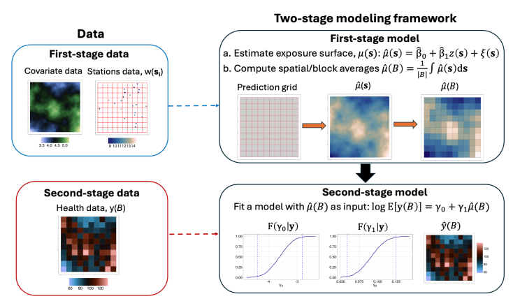
An example in spatial epidemiology is shown in Figure 1 (Blangiardo et al. [5], Lee et al. [20], Cameletti et al. [6], Liu et al. [25]). Here, the aim is to understand the link between case counts of a disease and some exposure variable, for example pollution level or meteorological variables. Data on case counts are areal, i.e., aggregated quantities over regions or blocks; while the exposure variable is spatially continuous and observed at a finite number of spatial points (e.g. weather stations). The first step consists of fitting a spatial model (first-stage model), which is then used to predict the exposure surface on a fine grid. Spatial averages of the predicted surface for each area/block are then computed. The next step is to fit a model (second-stage model) to link the case counts and the block estimates of exposures. A simple formulation of this two-stage model is as follows:
| (1) | |||
| (2) | |||
| (3) | |||
| (4) |
where is the true exposure surface, is a spatially correlated random field, is a known covariate, is the observed value of at a spatial location , is a measurement error term. denotes the observed count of the disease in block and is assumed to follow the Poisson distribution. The above model assumes that the counts are linked to via the spatial averages where is the size of block (Equation (4)). The model unknowns are the fixed effects , and the hyperparameters which include the error variance , and the parameters of the random field .
Simultaneous fitting of Equations (1)-(4), also referred to as a joint modeling approach, can be computationally challenging and expensive (Gryparis et al. [16], Liu et al. [25]). Moreover, the first-stage model is typically the most computationally demanding; thus, joint modeling can be inconvenient if there are several epidemiological models of interest (Liu et al. [25], Blangiardo et al. [5]). Equations (1) – (4) can be viewed as a model with covariate measurement error (Berry et al. [4]). Berry et al. [4] proposed to fit the equations simultaneously, which they refer to as a fully Bayesian approach. However, a potential problem with this approach is that it could cause potential ‘feedback’ effects, wherein the data influence and distort the model for , which consequently may compromise the relationship (Wakefield and Shaddick [48], Shaddick and Wakefield [37], Gryparis et al. [16]). This could happen when data to inform about are sparse (Gryparis et al. [16]) or due to model misspecification (Yucel and Zaslavsky [51]). One way to ‘cut’ the feedback between the two stages is by introducing a cut function in an MCMC algorithm (Plummer [32]). The cut function essentially simplifies the full conditional distribution of a graphical model into smaller modules that interact more weakly than in a full Bayesian analysis (Bayarri et al. [2], Spiegelhalter et al. [39]). However, this approach may not converge to a well-defined limiting distribution unless tempered transitions are introduced (Plummer [32]). In addition, it is well-known to be difficult to implement and computationally expensive (Chakraborty et al. [7]). Thus, a fully Bayesian approach may not be practical, especially with the increase in the volume of available and accessible data nowadays, which implies that fitting the first-stage model can be complex in itself. This problem has been approached using frequentist estimation methods as well (Lopiano et al. [26], Szpiro and Paciorek [41]).
Hence, a two-stage modeling framework, as illustrated in Figure 1, has often been used. Here, the first stage would fit Equations (1) and (2), providing estimates for , denoted as . Such estimates can be used to compute the spatial averages . In the second stage, serves as input in Equation (3), yielding posterior estimates of and . However, the predictions are subject to uncertainty from estimation error or model misspecification, which must be appropriately propagated to the second stage.
We argue that the two-stage modeling framework is often more practical or appropriate in several scenarios due to three main reasons. First, it offers an intuitive physical interpretation, as there is a unidirectional relationship between and (e.g., climate and pollution levels affect disease risks but not vice versa). Second, it is computationally efficient, particularly when the first-stage model is already complex. Third, it avoids potential feedback issues that can arise in fully Bayesian approaches.
While uncertainty propagation is intrinsic to a fully Bayesian approach, it must be explicitly accounted for in a two-stage modeling framework. The novelty of this work lies in validating different two-stage modeling approaches using the self-consistency property of Bayesian algorithms. This property holds if the data-averaged posterior is equal to the prior distribution (Geweke [13]). To test this, we use the simulation-based calibration (SBC) method (Talts et al. [43]), discussed in Section 3. The SBC method allows us to assess the correctness of a Bayesian algorithm and has a frequentist interpretation, since the results are viewed as the expected behavior averaged over all potential data outcomes. We also introduce a variation of SBC tailored for situations where some first-stage model parameters violate self-consistency, but the second-stage parameters are of primary interest. This is detailed in Section 3.2. Both the original and modified SBC methods are implemented in our experiments. As noted by Talts et al. [43], SBC is a crucial part of a robust Bayesian workflow that involves model building, inference, and model checking/improvement (Gelman et al. [12]).
Another significant contribution of this work is a new approach for uncertainty propagation in two-stage Bayesian models, referred to as the uncertainty method. This method introduces an error component in the second-stage model, which is assigned a Gaussian prior with zero mean and covariance matrix . It encodes the full uncertainty from the first-stage model. While this method has similarities to the prior exposure method (Cameletti et al. [6]), it incorporates the full covariance structure of the first-stage latent parameters. Unlike previous approaches (Chang et al. [8], Peng and Bell [31]), which use first-stage posterior results as priors in the second stage, our method explicitly adds a new model component to capture first-stage uncertainty. Additionally, we explore a low-rank approximation of the error component to handle high-dimensional spatial models, such as large spatio-temporal datasets. This results in two variants: the full uncertainty approach and the low-rank uncertainty approach. Both methods are particularly convenient in the framework of latent Gaussian models and when inference is performed using INLA.
Section 2 formally discusses the two-stage modeling framework and the uncertainty propagation problem. Section 2.1 reviews two current approaches: the crude plug-in approach and the resampling approach. Section 2.2 presents the proposed methods within the INLA framework, applied to spatial modeling contexts. Section 3 elaborates on the self-consistency property, the SBC method, and our proposed SBC variant. In Section 4, we validate four uncertainty propagation approaches: the crude plug-in approach, the resampling approach, the full approach, and the low rank approach through simulation experiments. These include a two-stage spatial model with Gaussian observations and point referenced data in the second stage (Section 4.1), and one with Poisson observations and areal data in the second stage (Section 4.2). We focus on the SBC results for the second-stage parameters, and , which are most affected by potential underestimation of posterior uncertainty in a two-stage framework. Finally, we demonstrate the proposed methods in a real-world application, which aims to link relative humidity (a climate variable) and Dengue case counts in the Philippines in August 2018 (Section 5). The paper concludes with insights and future directions in Section 6.
2 Uncertainty propagation problem
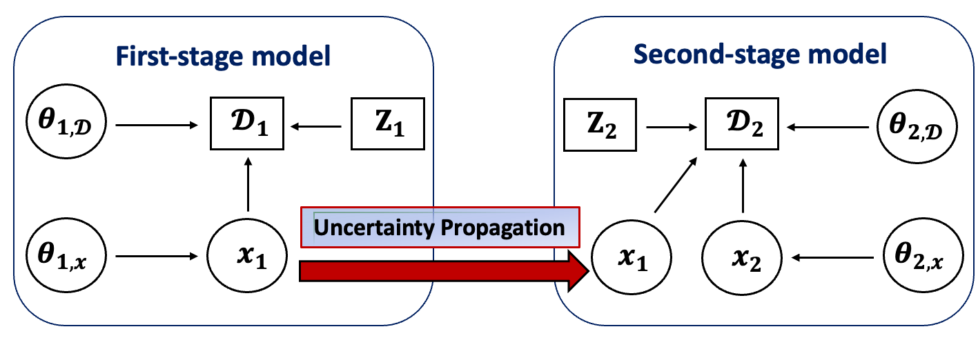
We assume that model inference for a physical process of interest is performed in two stages, as shown in Figure 2. The observed data is , partitioned into the first-stage data and second-stage data, respectively. First-stage inference is performed using only and without looking at , since for instance the health counts are not intended to inform the estimation of exposures or the health biomarkers causes the probability of survival and not the other way around. We model such process using a Bayesian hierarchical model. Let and be the latent parameters and hyperparameters linked to , respectively. We partition into , for which are the hyperparameters linked to , while are the hyperparameters linked to . Also, let be a set of fixed inputs/covariates. We assume that Similarly, let and be the latent parameters and hyperparameters linked to , respectively, and be a set of fixed inputs. The modeling framework in Figure 2 assumes that from the first-stage model is also linked to , so that we have This gives us the full data model:
Figure 2 considers , or some function of it, as an input when fitting the second-stage model. However, in practice, is unknown and needs to be estimated in the first stage. Hence, its uncertainty due to estimation error or model misspecification error needs to be correctly propagated into the second stage; otherwise, the standard errors of the second-stage model parameters may be underestimated. The end goal, therefore, is to correctly estimate the following posterior distributions:
-
•
The posterior distribution of the first-stage parameters, given by .
-
•
The posterior distribution of the second-stage parameters. For the plug-in method, this is given by , were denotes the posterior mean of from the first-stage model results. For the resampling method, this is given by .
When estimating the posterior distribution of the second-stage model, the uncertainty in needs to be accounted for, which is fundamentally the uncertainty propagation problem.
2.1 Current approaches
This section discusses two existing approaches to fit the two-stage model in Figure 2. Although not exhaustive, these approaches serve as benchmarks for comparison with our proposed approaches. Related methods, which use first-stage posteriors as priors for the second stage, are discussed in Section 2.2.
-
1.
Plug-in Method – Let be the posterior mean of estimated from the first-stage model. The crude plug-in method simply uses this as an input to the second stage. The linear predictor of the second-stage model is then:
(5) where is the link function, are model fixed effects, and is a vector-valued linear function . Note that Equation (5) can also include random effects. The estimated uncertainty in the second-stage posterior distribution, , is possibly underestimated since it fails to account for the uncertainty in .
-
2.
Resampling method – The resampling method, described in Algorithm 1, accounts for the uncertainty in the first-stage model in a natural way, but can be computationally expensive since it requires fitting the second-stage model several times.
Algorithm 1 Implementation of the resampling method
2.2 Proposed method – uncertainty
In this section, we present the proposed uncertainty method for uncertainty propagation. This approach avoids multiple runs of the Bayesian algorithm for the second-stage model, offering potential computational efficiency over the resampling method. The method shares similarities with MCMC algorithms used by Chang et al. [8], Peng and Bell [31], and Gryparis et al. [16], where the second-stage model is fitted using first-stage results as an informative prior. Two implementation approaches are noted in the literature: one that allows feedback by updating the prior distribution with second-stage data (Gryparis et al. [16], Chang et al. [8]), and another that cuts feedback by fixing the prior at each iteration (Peng and Bell [31]). Our method aligns with the latter, as we also cut feedback. It is also related to Cameletti et al. [6], but uniquely accounts for the full uncertainty in first-stage latent parameters via the matrix. We propose two versions: the full uncertainty method and the low rank uncertainty method, the latter being an approximation useful for large matrices, such as in spatio-temporal applications. Both methods are implemented within the INLA framework (Rue et al. [33], Van Niekerk et al. [45]) and demonstrated in spatial applications.
2.2.1 Full Q uncertainty method
In order to formally describe the proposed method, we first briefly describe the INLA methodology, with particular focus on how the matrix is computed. This is important since encodes the uncertainty in the latent parameters of the first-stage model, i.e., the uncertainty in (see Figure 2), which is then propagated to the second-stage model. The first-stage Bayesian hierarchical model is as follows:
The above is a latent Gaussian model since a Gaussian prior is assumed for the latent parameters . For inference, the needed quantities are the posteriors and . The estimated posterior marginal of , , is
where is the Gaussian approximation of , computed from a second-order expansion of the log-posterior density around its mode. In particular, is given by
| (6) |
where is the mean of the Gaussian approximation for a given , and is a sparse precision matrix which primarily depends on two components: the graph obtained from the prior of and the graph based on the mapping from to the linear predictors (Van Niekerk et al. [45]), and is also computed given . The marginal posterior of each element of are then calculated by integrating out using numerical integration.
The variance-covariance matrix in Equation (6) encodes the uncertainty in the latent parameters . Its inverse is what we refer to as the matrix, i.e., . We then use this information when fitting the second-stage model. In particular, in the second-stage hierarchical model, we introduce a new model component , which we call an error component. Its prior model is derived from Equation (6), i.e., . In practice, we propose to evaluate at the mode of . The predictor in the second stage is then given by
| (7) |
We call this approach the full uncertainty method.
In fitting Equation (7), the quantity is assumed to be fixed and known. Since is a linear function of , it follows that is also Gaussian. However, is also unknown and assigned a Gaussian prior; thus, Equation (7) is not a latent Gaussian model since the predictor involves a product of two components, each with a Gaussian prior. One way to fit the model is to linearize the predictor in Equation (7) using a first-order Taylor approximation as implemented in the R library inlabru (Lindgren et al. [24]). Another approach is to specify a grid of values for , and then fit Equation (7) conditional on each . All estimates are then combined using model averaging (Gómez-Rubio et al. [15]). A third approach is to fit the model using a hybrid INLA with MCMC or importance sampling approach. Here is estimated using sampling, while the rest of the parameters are estimated using INLA (Gómez-Rubio and Rue [14], Berild et al. [3]).
In the INLA framework, the model component in Equation (7) involves a scaling or precision parameter, say , for . We propose fixing the value of this scaling parameter at . Note that fixing this value to higher (lower) values implies a reduction (increase) in the uncertainty carried over from the first-stage model to the second-stage model. An approach for determining the optimal value of could be pursued in future work.
An application to spatial models
In spatial applications, the linear predictor in the first-stage model is a combination of fixed effects and a random field. In these scenarios, a common specification for the function in Equation (7) is as follows:
| (8) |
where are fixed effects and is a random field. An efficient method for estimating the random field is the stochastic partial differential equations (SPDE) approach (Lindgren et al. [23]). This approach provides a finite-dimensional but continuously-indexed approximation of Gaussian fields with Matérn covariance function. The discretization is defined on a mesh and expresses the approximation as
| (9) |
where is the number of mesh nodes or vertices, are basis functions chosen to be piecewise linear in each triangle, i.e., at vertex and otherwise, and are Gaussian-distributed weights. The approximation in Equation (9) is fully specified by the probability distribution of the weights , where is a sparse precision matrix. The speed of the computation depends on the resolution of the mesh, i.e., the number of mesh nodes . Using the SPDE approach, we can write Equation (8) as
where the latent parameter vector is , and is the mapping matrix from the mesh nodes to the observed data points. With the full uncertainty method, we use the posterior mean and the precision matrix from the Gaussian approximation in Equation (6). The linear predictor in the second-stage model is then specified as:
| (10) |
where , and are the model parameters; , and are known matrices; and is the error component with prior given by .
2.2.2 Low rank Q uncertainty method
A potential problem with the specification in Equation (10) is that when extending this to large spatio-temporal data, the dimension of scales linearly as the number of time points, which in effect also applies to the dimension of the error component . Thus, we propose a low rank approximation of , which then expresses Equation (10) as follows:
| (11) | ||||
| (12) |
where we have implicitly partitioned into , with being the fixed effects error component which is time-invariant, and is the spatial error component which varies in time. In Equation (11), is used to approximate , where is defined on a coarser mesh compared to the mesh used for , and is the appropriate projection matrix from the coarse mesh to the fine mesh.
The probability model for depends on the distribution of the weights at the coarser mesh, say , , being the dimension of . The probability model for is given by as stated in Theorem 2.1.
Theorem 2.1.
Suppose is defined on a discretization of dimension , i.e. , with probability model . Suppose we define a coarser discretization specified via the weights , such that . Then, the precision matrix of is given by and the probability model of is given by
Proof.
This is simply a generalized least squares problem, i.e., . This yields and ∎
3 Simulation-based calibration for model validation
We validate the uncertainty propagation methods discussed in Sections 2.1 and 2.2 using the simulation-based calibration (SBC) approach, originally proposed by Talts et al. [43] and based on ideas from Cook et al. [9]. The SBC method tests for the self-consistency property of Bayesian models, which states that the posterior distribution, averaged over all possible outcomes from the full generative model, is equal to the prior distribution. Formally, suppose is the prior model, is the observation density or probability mass function, and is the posterior distribution. The self-consistency property is stated as:
Any discrepancy between the prior model and the data-averaged posterior indicates an error in the Bayesian algorithm. The SBC method tests this property using rank statistics. It involves sampling from the data’s generative model and applying the Bayesian algorithm to each data replicate. Specifically, consider the following sequence of samples drawn from the Bayesian model:
If the Bayesian algorithm is correct, then for any one-dimensional function of the parameters, , where is the -space, the rank statistic of the prior sample relative to the posterior sample, given by
| (13) |
should be uniformly distributed across the integers .
Deviations from uniformity in the rank distribution provide insights into errors in the posteriors. A -shaped rank distribution suggests that the data-averaged posterior is overdispersed compared to the prior, meaning uncertainty is overestimated, violating Bayesian self-consistency. Conversely, a -shaped rank distribution indicates underdispersion, where the estimated posterior underestimates the true uncertainty. Asymmetry in the rank distribution reveals bias in the data-averaged posterior, deviating in the opposite direction relative to the prior distribution.
3.1 Implementation of SBC for the two-stage model
This section discusses how to implement the SBC in a two-stage modelling framework following Figure 2. We assume that , and , and that and are continuous spaces. The assumption of continuous spaces for the model parameters are crucial for the SBC method in Talts et al. [43] to work. For cases when some of the spaces are discrete, an SBC variant is proposed in Modrák et al. [28].
Following Equations (5), (10), and (11), we are interested in the posterior marginals of and , since these are the parameters which are potentially underestimated when the uncertainty in the first stage model is not properly propagated to the second stage. We use the individual parameters as test quantities to check that their uncertainty is correctly calibrated. Testing individual parameters allows the diagnosis of a large number of problems with posterior approximation (Modrák et al. [28]). However, Modrák et al. [28] also recommended the use of test functions which are data-dependent, such as the joint likelihood of the data, since there are large classes of problems which cannot be detected when the test quantities are functions only of the parameters. We have not considered such test functions in this work, but plan to do so in future work.
Algorithm 2 shows the steps to implement the SBC for a two-stage Bayesian model in Figure 2, where the test quantities are and . To test for the uniformity of the rank statistic in Equation (13), we primarily use the graphical approach in Säilynoja et al. [35], which generates simultaneous confidence bands for the difference between the empirical cumulative distribution function (ECDF) and the uniform CDF. The method is not sensitive to binning, does not require smoothing, and provides intuitive visual interpretation.
3.2 Variation in the SBC
In this section, we propose a variation of the SBC approach in a two-stage modeling framework. The motivation here is that the parameters of primary interest are the fixed effects of the second-stage model, namely and , and we want to avoid the influence of certain parameters of the first-stage model which may violate the self-consistency property for specific priors or model specification. As an example, some parameters in (Figure 2) may violate the self-consistency property. Hence, we propose Theorem 3.1, which derives the distribution of the rank statistic for an arbitrary unidimensional test function conditional on . This is then used as the theoretical basis for doing the SBC conditional on .
Theorem 3.1.
Let be the prior model, be the latent model, and be the observation density or probability mass function. Let be the latent space, be the -space, and be the -space, all continuous. Suppose is fixed. Let be a sample from the prior, i.e., , be a sample from the latent model, i.e., , and a sample from the observation model, i.e., . Suppose that the approximate posteriors from applying the Bayesian algorithm are and . Let and be independent samples from the posteriors, i.e., , and . Then, we have the following results:
-
(1)
For any uni-dimensional function , the distribution of the rank statistic
is .
-
(2)
For any uni-dimensional function , the distribution of the rank statistic
is .
The proof of Theorem 3.1 is in Section 1.1 of the Supplementary Material. Theorem 3.1 implies a variation in the implementation of the original SBC. Instead of sampling from the full data generative model, we fix the value of . In particular, the changes in Algorithm 2 only apply to Steps 1 – 3, which are the steps for generating data from the model. The changes are formalized in Algorithm 3. The remaining steps for doing the SBC conditional on are the same as the original SBC, i.e., the model inference is done without knowledge of and the test quantities for the SBC are and . Moreover, we extend Theorem 3.1 to the case where we condition on the entire hyperaparameter vector . This is formalized in Section 1.2 of the Supplementary Material, and which we refer to as Theorem 3.2.
4 Simulation experiments
We perform simulation experiments where we compare the different uncertainty propagation approaches on two two-stage models: one with Gaussian observations (Section 4.1) and one with Poisson observations (Section 4.2). For each model, we highlight the SBC results for and using both Algorithms 2 and 3.
4.1 A two-stage spatial model with Gaussian observations
In the first experiment, the first-stage latent process is given by , where and are fixed effects, is a known covariate, and is a Gaussian field with Matérn covariance function. The error-prone observed outcomes are , which follows the classical error model, i.e.,
| (15) |
The latent process is an input in the second-stage model, i.e.,
| (16) |
Here, represents observations at locations different from where is measured. This model belongs to the class of measurement error models because in Equation (16) is unobserved and needs to be estimated using Equation (15) (Berry et al. [4], Banerjee and Gelfand [1], Madsen et al. [27]). Figure LABEL:fig:res_twostage_gaussian_simdata shows a simulated observed locations for and where . Note that is also another latent field of interest.
We use INLA with SPDE representations of the spatial fields to fit this model. The first- and second-stage latent parameters are and , respectively. The are the Gaussian weights of the SPDE approximation (Lindgren et al. [23]), i.e., where , are basis functions as discussed in Section 2.2. Moreover, the first-stage hyperparameters are , where and are the marginal variance and range parameter of the random field , respectively. The second-stage hyperparameter is .
We used Gaussian priors for the fixed effects: ; and penalized-complexity (PC) prior for and (Fuglstad et al. [11], Simpson et al. [38]). A PC prior for and penalizes deviation from the base model of zero variance. The formulation requires the user to specify a constant and a probability value such that . This is equivalent to the prior , where the rate parameter determines the magnitude of the penalty, with higher values corresponding to higher penalty. In particular, the PC priors for and are specified as and . For the Matérn parameters, we used a joint normal prior for and (Lindgren and Rue [22]), where
| (17) | ||||
| (18) |
In particular, we have . This prior specification implies that the plausible values for the Matérn parameters are and .
In doing the SBC, we fixed the spatial locations of and for all the data replicates which is shown in Figure LABEL:fig:res_twostage_gaussian_simdataa. The covariate field was simulated from a Matérn process with range of 0.6, standard deviation of 2, and mean-squared differentiability parameter of 1. This is fixed for all data replicates since is a known quantity in the model. The random field was also simulated from a Matérn process, with range and marginal standard deviation . It varies for the different data replicates since this is an unknown quantity which needs to be estimated.
We compare four uncertainty propagation approaches: plug-in, resampling (with resamples), full , and low rank uncertainty. The mesh used to fit the full uncertainty method is shown in Figure LABEL:fig:res_twostage_spatial_Gaussian_meshesa. Here, the maximum triangle edge lengths for the inner domain and the outer extension are 0.04 and 0.1 units, respectively. We use the same mesh to simulate and estimate . For the low rank approach, we explored two meshes (A and B) with different level of coarseness: for mesh A (Figure LABEL:fig:res_twostage_spatial_Gaussian_meshesb), the maximum edge lengths are 0.05 and 0.2 units, while for the coarser mesh B (Figure LABEL:fig:res_twostage_spatial_Gaussian_meshesc) (low rank mesh B), they are 0.1 and 0.25, respectively. The number of nodes is for the full mesh, for mesh A, and for mesh B.
Figure LABEL:fig:res_twostage_spatial_Gaussian_p_k shows the ECDF difference plot of the normalized ranks for and from 1000 data replicates using Algorithm 2 (corresponding histograms are in Figure 7 of the Supplementary Material). Results show that for the plug-in method, the hypotheses of uniform distribution of the ranks is rejected for both and (Figure LABEL:fig:res_twostage_spatial_Gaussian_p_ka). In addition, the -shaped histogram (Supplementary Material) reveals an underestimation of the posterior variance. The resampling method and the two proposed methods do not show deviations from uniformity, not even with the low rank approach using the coarser mesh B. This suggests that both the resampling approach and the proposed methods correctly capture the posterior uncertainty of and .
Although the primary focus is on these parameters, we also examined the histogram and ECDF difference plot of the normalized ranks for all first-stage model parameters. Section 2.1 in the Supplementary Material presents the SBC results for the first-stage model using Algorithm 2. The results show a uniform distribution of for all first-stage model hyperparameters, except for which is slightly -shaped. This motivates the use of Algorithm 3, based on Theorem 3.1, where SBC is applied conditional on . Moreover, three mesh nodes fail the Kolmogorov-Smirnov test for uniformity at 10% significance level (see Figure 1 in Section 2.1 of the Supplementary Material).
The results from Algorithm 3 are shown in Sections 2.2 and 2.4 in the Supplementary Material. The conclusions are consistent with those from Algorithm 2, i.e., the plug-in method underestimates the posterior uncertainty of and , while the resampling method and the proposed methods are also correct, althought there may be slight underestimation with the low rank approach. Finally, we also attempted to perform the SBC on a non-spatial two-stage model, i.e., similar to Equations (15) and (16) but without the spatial field . We used both the INLA and no U-turn sampler (NUTS) (Hoffman et al. [17]). The results, which are given in Section 5.1 of the Supplementary Material, also show that the plug-in method underestimates the posterior uncertainty of both and , while the resampling and the methods are correct. Note that the method is implemented only using the INLA method.
4.1.1 Illustration with simulated data
To gain additional insights, we analyze in detail one simulated data from the previous section with true values of the parameters as follows: , and . Figure LABEL:fig:res_twostage_gaussian_simdata shows: (a) the spatial locations for the data and , (b) the simulated field , and (c) the simulated field which we estimate using the different uncertainty propagation approaches. The posterior means of (Figure LABEL:fig:res_spatial_twostage_gaussian_predfield_s2a) are all very similar and close to the truth (Figure LABEL:fig:res_twostage_gaussian_simdatac). Posterior standard deviations (Figures LABEL:fig:res_spatial_twostage_gaussian_predfield_s2b) are smallest, as expected, for the plug-in method. The resampling method resulted in the highest overall uncertainty, while the full uncertainty method produced posterior uncertainties nearly identical to those of the resampling method. The posterior uncertainty from the low-rank method is lower than that of the full method, but higher than the uncertainty from the plug-in method.
Figure 5 shows the marginal posterior CDFs of and from the same simulated data. The plug-in method has the smallest posterior uncertainty for both parameters, but the difference is more apparent for . The resampling method has the highest posterior uncertainty, while the proposed methods provide a middle ground between the plug-in and resampling method. The posterior estimates from the full method and the low rank method are very similar.

Figures LABEL:fig:res_spatial_gaussian_twostage_ecdfs_varylogprec_fullQa and LABEL:fig:res_spatial_gaussian_twostage_ecdfs_varylogprec_fullQb show a comparison of the estimated posterior CDFs of and , respectively, for different fixed values of the scaling parameter of the error component using the full method, as discussed in Section 2.2. The results show that as the log precision becomes larger, the estimated CDFs for and approaches the estimated CDFs of the plug-in method. Also, as the log precision value becomes smaller, the estimated CDFs deviate more from the estimated CDFs of the plug-in method, i.e., the posterior uncertainty becomes larger. The same insights are true from the results of the low rank method (see Section 2.5 of the Supplementary Material).
In terms of computational time, the crude plug-in method took 2.98 seconds to fit the second-stage model, while the full method took 9.82 seconds. The low rank approach took 13.97 seconds with mesh A, and 5.80 seconds with mesh B. This suggests that using a coarse mesh with the low rank does not always lead to reduced computational time. A plausible reason for this is that the linear predictor of the low rank method, as shown in Equations (11) and (12), is more complex and involves additional operations compared to the linear predictor of the full method in Equation (10). We have the computational advantage of the low rank approach from using a coarse enough mesh, similar to mesh B in Figure LABEL:fig:res_twostage_spatial_Gaussian_meshesc. Lastly, the resampling method with , took 36.12 seconds using parallel computing with the mclapply() function in R.
The results from the SBC provide evidence that the plug-in method underestimates the posterior uncertainty, while the resampling method is correct. The full and the low rank methods are also expected to give correct posteriors for and . The computational benefits from the low rank method potentially depends on the coarseness of the mesh for the error component.
4.2 A two-stage spatial model with Poisson observations
In this section, we perform the SBC in a two-stage spatial model with Poisson observations. We consider two model specifications: the first one, called the classical specification, is similar to Equations (3) and (4) in Section 1. Here, the second-stage model specifies the log mean of the Poisson counts in each block as linear with respect to the block averages of . This approach is often used in such spatial misalignment problems since it is straightforward to implement (Blangiardo et al. [5], Lee et al. [20, 21], Liu et al. [25], Villejo et al. [46], Cameletti et al. [6], and Zhu et al. [52]). The second, named new specification, introduces a spatially continuous latent intensity field for the Poisson counts, which is then linked to the log mean in a nonlinear way (Lindgren et al. [24]). This approach better represents the physical process by assuming that the observed Poisson counts are function of the averages of a latent intensity field over the areas. Although this results in a highly nonlinear model, it can be efficiently fitted using an approximate iterative method with INLA. This method extends the applicability of INLA beyond the linear predictor framework to accommodate more complex functional relationships and can be implemented with the inlabru library in R (Lindgren et al. [24]).
4.2.1 Classical specification
The first-stage latent model is similar to the one in Section 4.1, so that and the observed data } also follows the classical error model. The latent process is an input in the second-stage model as follows:
The above model is closely related to the joint model in Equations (1) – (4), but here we have additional quantities which are introduced as an offset in order to account for the different sizes of the blocks . For example, in spatial epidemiology where is the observed disease count, is the expected number of cases and are computed using the size and demographic structure of the population in block (Lee [19]). In this specification, is interpreted as the disease rate or risk (Lee et al. [20], Blangiardo et al. [5]). We used the INLA-SPDE approach to fit the model. The second-stage data is . Similar to Section 4.1, the first-stage and second-stage model latent parameters are and , respectively. The first-stage model hyperparameters are . There are no second-stage model hyperparameters.
We simulate and as in Section 4.1. The spatial locations of the first-stage observations and the meshes for the full and low rank are also as in Section 4.1. The configuration of the Poisson blocks is shown in Figure LABEL:fig:res_spatial_twostage_poisson_classical_illustrationd. We used the following priors for the fixed effects: We used the PC prior for , particularly , and the same joint log Gaussian prior for the Matérn parameters from Section 4.1. Again, we consider four methods of uncertainty propagation: plug-in method, resampling method, full method, and the low rank method.
Figure LABEL:fig:res_twostage_poisson_p_k_classical_ecdfdiff shows the plot of the ECDF differences of for and using Algorithm 2 with 1000 data replicates (corresponding histograms are in Section 3.3 of the Supplementary Material). Again, the plug-in method appears to underestimate the true posterior uncertainty for both parameters, while the resampling and the full uncertainty methods do not show deviations from uniformity. The two versions of the low rank approach (mesh A and mesh B) show slight deviation from uniformity, but not as bad as the plug-in method. Results for the first-stage model parameters using Algorithm 2 are shown in Section 3.1 of the Supplementary Material. As in Section 4.1, the histogram of the normalized ranks for is -shaped. Moreover, there are some mesh nodes which also fail the uniformity test using the KS test at 10% significance level. Results using Algorithm 3 are shown in Section 3.2 and Section 3.4 in the Supplementary material for the first-stage and second-stage model parameters, respectively. The results are coherent with those from Algorithm 2.
Similar to Section 4.1, initial validation was done for a non-spatial two-stage model, i.e., without the spatial field in the first stage. The results for both INLA and NUTS are in Section 5.2 of the Supplementary Material. The results are consistent with previous results that the plug-in method underestimates the posterior uncertainty of both and , while the resampling and the proposed method are correct.
4.2.2 New specification
For the new model specification, the second-stage model is as follows:
The first-stage model is the same as the one used for the classical specification; but here we assume that is linked to another latent intensity field which we denote by . We use the same covariate , the same spatial locations for the first-stage data, and the same configuration of the block/areas for the Poison outcomes as the classical specification. We also use the same priors for all model parameters, and compare the same uncertainty propagation methods.
Figure LABEL:fig:res_twostage_poisson_p_k_logsumexp_ecdfdiff shows the plot of the ECDF differences of the normalized ranks for and using Algorithm 2 and from 1000 data replicates. Histograms are provided in Section 3.5 of the Supplementary Material. The results show that the plug-in method underestimates the true posterior uncertainty for both parameters and introduces bias in the posterior distribution of . The resampling method correctly captures the posterior for , but shows some bias for , though less severe than the plug-in method. The full and low rank methods also show potential bias for on the same direction as the plug-in and resampling method. Moreover, the ECDF difference plot reveals a slight deviation from uniformity for , though less pronounced than that of the plug-in method. This suggests that the -based methods strike a balance between the plug-in and the resampling method. Results from Algorithm 3, shown in Section 3.6 of the Supplementary Material, align with the insights from Algorithm 2.
4.2.3 Illustration with simulated data
To illustrate the previous insights from the SBC, we simulate a data from both model specifications. We set the true values of the parameters as follows: . Moreover, we keep the spatial locations of the first-stage observations as in Section 4.1 (Figure LABEL:fig:res_twostage_gaussian_simdataa), and set for all blocks.
Figure LABEL:fig:res_spatial_twostage_poisson_classical_illustrationa shows the simulated . The classical specification aggregates over the blocks, which is shown in Figure LABEL:fig:res_spatial_twostage_poisson_classical_illustrationb. The corresponding are in Figure LABEL:fig:res_spatial_twostage_poisson_classical_illustrationc, while the simulated Poisson outcomes are in Figure LABEL:fig:res_spatial_twostage_poisson_classical_illustrationd. For the new specification, we first compute the latent intensity field which is then aggregated over the blocks to yield . The simulated and for the new specification are shown in Figure 21 in the Supplementary Material.
Figures LABEL:fig:res_spatial_twostage_poisson_estimatesa and LABEL:fig:res_spatial_twostage_poisson_estimatesb show the estimated marginal posterior CDFs of and for the classical specification and new specification, respectively. For both model specifications, the plug-in method evidently has the smallest posterior uncertainty among the four approaches. The resampling method and the -based methods have very similar posterior results. The posterior median for using the new model specification is slightly overestimated, but is well within the 95% credible interval. The results from this specific simulated data are consistent with the SBC results.
Figures LABEL:fig:res_spatial_twostage_poisson_logsumexp_pred_lambda_sda and LABEL:fig:res_spatial_twostage_poisson_logsumexp_pred_lambda_sdb show the posterior standard deviations of and , respectively, using the new model specification and for the different uncertainty propagation approaches. It is evident that the plug-in approach generally has the smallest posterior uncertainty. The resampling method and the -based methods have quite similar results, although the low rank method with a very coarse mesh has slightly smaller uncertainty estimates in some areas. The corresponding posterior means of and are shown in Figure 23 of Section 3.7 in the Supplementary Material. The posterior means of both and from the four uncertainty propagation approaches are very similar to the simulated truth. Moreover, the results from the classical model specification are shown in Figure 22 in the Supplementary Material. The results also show the same insights as the new model specification, i.e., the plug-in method has the smallest posterior uncertainty, while the resampling method and the -based method have similar results.
Table 1 shows the computational time (in seconds) for the different estimation approaches on the simulated data examples. For both the classical and new model specification, the plug-in method has the fastest computing time. The resampling method took the longest time for the classical model, while the full approach had a significant reduction in the computational time. In addition, the low rank (mesh A) took longer to run than the full method, but the low rank (mesh B) was faster than the previous two. This is consistent with the results from the simulated data example in Section 4.1, which show that the coarseness of the mesh for the error component is crucial in terms of the reduction in the computational time. On the other hand, for the new model specification, the full method took the longest computational time. The new model specification is a highly non-linear model, and introducing an error component all the more increases the model complexity; hence, making it plausible for the model fitting to even take longer. On the other hand, the low rank approach (both mesh A and mesh B) significantly reduced the computational time.
| Method | Classical specification | New specification |
|---|---|---|
| Plug-in | 3.04 | 4.64 |
| Resampling | 44.11 | 95.18 |
| Full | 14.28 | 110.76 |
| Low rank (mesh A) | 25.20 | 76.43 |
| Low rank (mesh B) | 6.78 | 20.38 |
The results for the two-stage Poisson models show that the plug-in method is expected to underestimate the posterior uncertainty in and . On the other hand, the resampling approach is expected to be correct. However, there is a potential bias for the intercept with the new model specification. The -based methods provide a middle ground between the plug-in method and the resampling method, but the gain in the computational time depends on the coarseness of the mesh for the error component. For the new model specification, which is a highly non-linear model, using a very fine mesh for the error component may not be recommended since doing model fitting could potentially take a longer time than the resampling approach.
5 Real data application
This section illustrates the proposed method in a real data application, which aims to link relative humidity (RH) and Dengue fever cases in the Philippines for August 2018. Dengue fever is an infectious disease common in tropical countries, and is caused by a virus transmitted by Aedes aegypti and Aedes albopictus, also known as yellow fever mosquito and Asian tiger mosquito, respectively. The association between climate variables and Dengue has been extensively studied (Murray et al. [29], Naish et al. [30], Lee et al. [21], Stolerman et al. [40]). In particular, relative humidity is known to increase the risks of Dengue since high humidity enhances reproduction and breeding, and increases survival and lifespan of mosquitoes (Thu et al. [44], Murray et al. [29], Naish et al. [30]).
5.1 Data
Monthly averages of relative humidity for August 2018 from 56 weather synoptic stations in the Philippines were provided by the Philippine Atmospheric, Geophysical and Astronomical Services Administration (PAGASA) (Figure LABEL:fig:data_applicationa). For each of the 82 provinces, the Epidemiological Bureau of the Department of Health provided the counts of Dengue fever (Figure LABEL:fig:data_applicationb). The standardized incidence ratios (SIR), computed as the observed divided by the expected cases, are shown in Figure LABEL:fig:data_applicationc. The expected cases are derived using national rates and via internal standardization (Waller and Carlin [49]). In particular, if and is the national rate and size of province , respectively, then the expected cases for the province is . The SIR indicates the relative excess in the incidence of the disease with respect to what might have been expected based on the reference national rates (Schoenbach and Rosamond [36]).
5.2 Model
We perform the inference in a two-stage modelling framework. The first stage models RH, while the second stage models the Dengue health counts using information from the first-stage model as an input.
-
•
First-stage model – Suppose is the log true relative humidity level at an arbitrary spatial location . We assume the following latent process:
where is a Matérn field and are fixed effects. We assume that the observed values at the weather stations follow the classical error model, i.e., and The temperature field is assumed to be known using the predicted values from the climate data fusion models in Villejo et al. [47].
-
•
Second-stage model – We consider both the classical and new specification in Section 4.2. Suppose and are the observed and expected Dengue cases in province , respectively. We assume that . This implies that , so that the disease risk is also interpreted as the model-based estimate of the SIR. For the classical specification, we assume that
where is an area-specific effect which we model as . For the new specification, we have:
We use the INLA-SPDE approach to fit the model. The mesh, with 1077 nodes, used to estimate the the Matérn field is shown in Figure LABEL:fig:application_stageone_fields_spde_highpreca. We use vague priors for the fixed effects and , and a joint normal prior (Equations (17) and (18)) for the Matérn parameters. In particular, we use . This implies that a plausible range of values for the range parameter is from 110 km to 800 km, which are consistent with the estimates in Villejo et al. [47]. Moreover, we set the plausible range of values for the marginal standard deviation as 0.2683 to 14.65, based on the empirical standard deviation of RH which is 5.37.
We compare the posterior estimates of and from the four uncertainty propagation approaches under consideration: plug-in, resampling, full , and low rank approach. In this case study, there is no strong motivation for the low rank approach since the dimension of the latent parameters is not large. Nonetheless, we explore the low rank approach in order to have a full comparison with the other approaches. Figure LABEL:fig:application_stageone_fields_spde_highprecb shows the mesh for the error component of the low rank approach, which has 546 nodes.
5.3 Results
5.3.1 First-stage model results
Figures LABEL:fig:application_stageone_fields_spde_highprecc and LABEL:fig:application_stageone_fields_spde_highprecd show the estimated posterior mean and standard deviation of the relative humidity field. The posterior estimates of the parameters are reported in Table 1 of Section 4 in the Supplementary Material. Both elevation and temperature appear to be significant predictors in the model. The northwestern section of the country has high relative humidity levels compared to most of the eastern section. This is consistent with the climate dynamics of the country (Flores and Balagot [10], Kintanar [18]).
5.3.2 Second-stage model results
In spatial epidemiology, it is usually more useful to interpret the multiplicative change in the disease risk, referred to as a rate ratio (RR) or relative risk, associated with one SD change in the exposure variable, which is relative humidity in this application. Figure LABEL:fig:CIwidth_dataapplication2a shows the estimated RR and the 95% CI (in dashed lines) associated with one SD change in RH. The actual 95% CIs are shown in Figure 25 of the Supplementary Material. The results show that for a one SD change in RH, the risk of Dengue approximately doubles. This is consistent with several studies which have shown a positive association between RH and the risk of Dengue (Thu et al. [44], Murray et al. [29], Naish et al. [30]). The width of the CIs from Figure LABEL:fig:CIwidth_dataapplication2 does not seem to be too different, but this is the typical length of the CIs in spatial epidemiology literature (Blangiardo et al. [5], Liu et al. [25], Lee et al. [20]). Also, both and are in the log risk scale, so that these differences are not negligible. We also computed the RR for other -units change in RH. In particular, we considered , where 5.4 corresponds to one SD in RH. The results are shown in Figure LABEL:fig:CIwidth_dataapplicationa. The figure shows that the CI widths in the RR are not too different when the magnitude of the change in the RH is small, but the difference in the CIs become more apparent when the change in RH is large. The posterior estimates for and the 95% CI widths for the different uncertainty propagation approaches are shown in Figure LABEL:fig:CIwidth_dataapplication2b and LABEL:fig:CIwidth_dataapplicationb, respectively. Figures 24a and 24b in the Supplementary Material show the estimated marginal CDFs of and for the classical and new specification, respectively, while the point estimates and 95% CI are shown in Tables 2 and 3 in Section 4 of the Supplementary Material. The resampling method and the two proposed methods have slightly larger posterior uncertainty than the plugin method for . The differences in the posterior uncertainty for are more apparent.
Figure LABEL:fig:CIwidth_dataapplication2 shows some differences in the posterior results among the four uncertainty propagation approaches. The posterior mean and the lower limit of the 95% CI of the RR for the resampling method is the lowest among the four uncertainty propagation approaches. This attenuation to the null risk of one is also observed in Lee et al. [20] and Liu et al. [25], where they argue that it is due to the posterior predictive distribution of the first-stage model outweighing the spatial (or spatio-temporal) variation in the data, which results in the estimated effects being washed away. Even so, we also see that the posterior mean for from the resampling method is the highest, so that both parameters balance each other out when calculating the log risks, . This is the same observation, although in the opposite direction, from the results of the -based methods, where the posterior mean of is relatively high, but the posterior mean for is relatively low. This observed push and pull between the two parameters explains why the estimated posterior means of for the four uncertainty propagation methods are very similar, as shown in Figure LABEL:fig:predicted_modelSIRsa for the classical specification and Figure 26 of Section 4 in the Supplementary Material for the new specification. Moreover, the estimated disease risks look very similar to the computed SIRs in Figure LABEL:fig:data_applicationc. The corresponding posterior SDs are shown in Figure LABEL:fig:predicted_modelSIRsb for the classical specification and Figure 27 in the Supplementary Material for the new specification. The differences in the posterior SDs are more apparent in the northern part of the country where the estimated risks are very high. The results show that the two proposed methods gave the highest posterior uncertainty, while the plug-in method has the lowest posterior uncertainty.
6 Conclusions
This work addresses the problem of uncertainty propagation in two-stage Bayesian models. This approach is appropriate for scenarios when there is a clear one-directional physical relationship between the two models, e.g., climate affects Dengue cases or air pollution affects respiratory diseases. Also, it is a practical approach when the first-stage model is already complex in itself; for example, it might involve fitting a complex data fusion model (Villejo et al. [46]). In addition, a two-stage modeling framework avoids the potential unwanted feedback effects present in fully Bayesian approaches (Wakefield and Shaddick [48], Shaddick and Wakefield [37], Gryparis et al. [16]). The drawback of the two-stage modeling framework is that uncertainty is not automatically propagated between the two models.
In this paper, we validate different uncertainty propagation approaches for two-stage models by testing the self-consistency property of Bayesian models using the simulation-based calibration (SBC) method of Talts et al. [43]. In particular, we investigated the correctness of two commonly used methods for two-stage modeling: the plug-in method and the resampling method. In addition, we also explored a new method called the uncertainty method. This introduces a new model component, called an error component, in the second-stage model. The error component is given a Gaussian prior with mean zero and precision matrix , derived from the Gaussian approximation of the latent parameters of the first-stage model. The matrix can be of high dimension (for example in large spatio-temporal applications); hence, we also proposed a low rank approximation of the matrix. We then have two versions of the proposed method: the full method and the low rank method. The uncertainty method is implemented using the INLA methodology, but we believe that the same idea can be used in other Bayesian inference approaches like MCMC. We plan to explore this in a future work.
We also proposed a modification of the SBC method of Talts et al. [43] to address challenges specific to two-stage Bayesian models. Here, the SBC algorithm is implemented conditional on fixed values of certain first-stage hyperparameters. This approach ensures that the evaluation focuses on the second-stage model parameters, avoiding the influence of first-stage parameters that may violate the self-consistency property. Results from both the original SBC and the conditional SBC confirm that the plug-in method underestimates the posterior uncertainty of the second-stage model parameters, while the resampling method provides correct uncertainty estimates. The proposed -based methods also produce correct posterior uncertainty estimates, although results indicate that the coarseness of the approximation can affect the accuracy of the approximate posteriors and the computational cost. In this work, we considered the individual parameters as test functions. The use of test functions which are data-dependent can be done in future work.
The computational efficiency of the -based methods depends on the coarseness of the mesh for the error component. For the new specification of the Poisson model, the full method required longer computational time compared to the resampling method. This is because the -based methods introduce an additional model component, significantly increasing model complexity and making fitting more computationally intensive, particularly for the highly nonlinear Poisson model. Nevertheless, a sufficiently coarse mesh in the low rank method can address this challenge while maintaining correctness. Moreover, the low rank approach may also take longer to run compared to the full method if the resolution of the approximation is not coarse enough. The reason for this is that the predictor expression of the second-stage model which implements the low rank approach involves more matrix operations, which may potentially increase the computational requirements for model estimation.
Some aspects of the uncertainty method require further investigation. Firstly, we fixed the scaling parameter of the matrix to 1, but this choice may not be optimal. When the scaling parameter is estimated rather than fixed, the results showed that its estimated value tends to be very large. This behavior implies an increased confidence in the first-stage posterior estimates, effectively reducing the uncertainty in the error component, and consequently producing narrower uncertainty estimates for the second-stage model parameters. Our simulation experiments revealed that as the fixed value of the scaling parameter decreases, the posterior uncertainty of the second-stage model parameters widens and deviates more significantly from the crude plug-in method. Conversely, when the scaling parameter increases, the posterior uncertainty narrows, approaching the uncertainty estimates produced by the plug-in method. Despite this, the SBC results indicated that fixing the scaling parameter to 1 appears appropriate, as it did not violate the self-consistency property of the model. Nevertheless, further work is needed to determine whether this choice is indeed optimal.
Secondly, the low rank method requires a more thorough investigation. We hypothesize that the coarser the approximation to the matrix, the more likely it becomes that the self-consistency of the model is violated. We have not properly explored and investigated the breakdown point of the low rank approximation of . This breakdown point is likely influenced by several factors, including the smoothness of the random field and the relative proportion of variability in the response variable explained by the fixed covariates versus the random field. A deeper understanding of these dependencies is essential to ensure the robustness of the low rank approximation. Thirdly, we used the empirical Bayes approach to fit the models in both the simulation experiments and data application. This implies that the matrix is computed at the mode of the first-stage model hyperparameters. If another numerical integration strategy is chosen by the user when implementing INLA, such as a grid approach, there will be several matrices, one for each of the integration point for the model hyperparameter. In this scenario, we propose the use of the weighted average of the matrices, where the weights are the same integration weights from the numerical integration used to compute the approximated posteriors of the latent parameters.
The SBC method is a computational method for testing the self-consistency property of Bayesian models. It is implemented in a specific Bayesian model, prior specification, and Bayesian inference algorithm. For this work, we validated simple two-stage spatial models. However, in practice, the models we investigate are more complex. For the toy models considered in this work, we have shown and illustrated that the crude plug-in method indeed underestimates the posterior uncertainty of the second-stage model parameters. For more complex models, this underestimation of the posterior uncertainty will also be highly likely true. Moreover, our results also showed that the resampling method is correct. We also think that the resampling method should also be able to compute the correct posterior uncertainty for more complex models. However, the only way to exactly know this is to implement the SBC method for every new Bayesian model specification, new prior specification, and new Bayesian algorithm. This aligns with the proposal in Talts et al. [43] that the SBC should be an integral part of a robust Bayesian workflow (Gelman et al. [12]). However, the SBC method is very computationally expensive and might not be a practical route in many contexts. Therefore, we propose that a more practical approach to perform a two-stage model analysis is to implement different uncertainty propagation approaches and compare the obtained posterior uncertainties. The crude plug-in method is definitely the easiest strategy, but the results of which should only be taken as an initial understanding of the model. A more comprehensive analysis should involve doing resampling and other approaches, such as the proposed uncertainty method when the Bayesian inference is done using INLA. Implementing different uncertainty propagation strategies allows an objective comparison of the estimated posterior uncertainties, which would then help uncover interesting model insights and guide both the statistical and practical interpretation of the results.
Statements and Declarations
Competing Interests: The authors have no competing interests to declare that are relevant to the content of this article. All authors certify that they have no affiliations with or involvement in any organization or entity with any financial interest or non-financial interest in the subject matter or materials discussed in this manuscript.
Funding: No funding was received for conducting this study.
References
- Banerjee and Gelfand [2002] S Banerjee and AE Gelfand. Prediction, interpolation and regression for spatially misaligned data. Sankhyā: The Indian Journal of Statistics, Series A, pages 227–245, 2002.
- Bayarri et al. [2009] MJ Bayarri, JO Berger, and F Liu. Modularization in bayesian analysis, with emphasis on analysis of computer models. Bayesian Analysis, 4(1):119–150, 2009.
- Berild et al. [2022] Martin Outzen Berild, Sara Martino, Virgilio Gómez-Rubio, and Håvard Rue. Importance sampling with the integrated nested laplace approximation. Journal of Computational and Graphical Statistics, 31(4):1225–1237, 2022.
- Berry et al. [2002] Scott M Berry, Raymond J Carroll, and David Ruppert. Bayesian smoothing and regression splines for measurement error problems. Journal of the American Statistical Association, 97(457):160–169, 2002.
- Blangiardo et al. [2016] Marta Blangiardo, Francesco Finazzi, and Michela Cameletti. Two-stage bayesian model to evaluate the effect of air pollution on chronic respiratory diseases using drug prescriptions. Spatial and spatio-temporal epidemiology, 18:1–12, 2016.
- Cameletti et al. [2019] Michela Cameletti, Virgilio Gómez-Rubio, and Marta Blangiardo. Bayesian modelling for spatially misaligned health and air pollution data through the inla-spde approach. Spatial Statistics, 31:100353, 2019.
- Chakraborty et al. [2023] Atlanta Chakraborty, David J Nott, Christopher C Drovandi, David T Frazier, and Scott A Sisson. Modularized bayesian analyses and cutting feedback in likelihood-free inference. Statistics and Computing, 33(1):33, 2023.
- Chang et al. [2011] Howard H Chang, Roger D Peng, and Francesca Dominici. Estimating the acute health effects of coarse particulate matter accounting for exposure measurement error. Biostatistics, 12(4):637–652, 2011.
- Cook et al. [2006] Samantha R Cook, Andrew Gelman, and Donald B Rubin. Validation of software for bayesian models using posterior quantiles. Journal of Computational and Graphical Statistics, 15(3):675–692, 2006.
- Flores and Balagot [1969] JF Flores and VF Balagot. Climate of the philippines. in: Arakawa, h. (ed.). Climate of Northern and Eastern Asia, World Survey of Climatology, 8, 1969.
- Fuglstad et al. [2019] Geir-Arne Fuglstad, Daniel Simpson, Finn Lindgren, and Håvard Rue. Constructing priors that penalize the complexity of gaussian random fields. Journal of the American Statistical Association, 114(525):445–452, 2019.
- Gelman et al. [2020] Andrew Gelman, Aki Vehtari, Daniel Simpson, Charles C Margossian, Bob Carpenter, Yuling Yao, Lauren Kennedy, Jonah Gabry, Paul-Christian Bürkner, and Martin Modrák. Bayesian workflow. arXiv preprint arXiv:2011.01808, 2020.
- Geweke [2004] John Geweke. Getting it right: Joint distribution tests of posterior simulators. Journal of the American Statistical Association, 99(467):799–804, 2004.
- Gómez-Rubio and Rue [2018] Virgilio Gómez-Rubio and Håvard Rue. Markov chain monte carlo with the integrated nested laplace approximation. Statistics and Computing, 28:1033–1051, 2018.
- Gómez-Rubio et al. [2020] Virgilio Gómez-Rubio, Roger S Bivand, and Håvard Rue. Bayesian model averaging with the integrated nested laplace approximation. Econometrics, 8(2):23, 2020.
- Gryparis et al. [2009] Alexandros Gryparis, Christopher J Paciorek, Ariana Zeka, Joel Schwartz, and Brent A Coull. Measurement error caused by spatial misalignment in environmental epidemiology. Biostatistics, 10(2):258–274, 2009.
- Hoffman et al. [2014] Matthew D Hoffman, Andrew Gelman, et al. The no-u-turn sampler: adaptively setting path lengths in hamiltonian monte carlo. J. Mach. Learn. Res., 15(1):1593–1623, 2014.
- Kintanar [1984] Roman L Kintanar. Climate of the philippines. 1984.
- Lee [2011] Duncan Lee. A comparison of conditional autoregressive models used in bayesian disease mapping. Spatial and spatio-temporal epidemiology, 2(2):79–89, 2011.
- Lee et al. [2017] Duncan Lee, Sabyasachi Mukhopadhyay, Alastair Rushworth, and Sujit K Sahu. A rigorous statistical framework for spatio-temporal pollution prediction and estimation of its long-term impact on health. Biostatistics, 18(2):370–385, 2017.
- Lee et al. [2021] Sophie A Lee, Theodoros Economou, Rafael de Castro Catão, Christovam Barcellos, and Rachel Lowe. The impact of climate suitability, urbanisation, and connectivity on the expansion of dengue in 21st century brazil. PLoS Neglected Tropical Diseases, 15(12):e0009773, 2021.
- Lindgren and Rue [2015] Finn Lindgren and Håvard Rue. Bayesian spatial modelling with r-inla. Journal of statistical software, 63(19), 2015.
- Lindgren et al. [2011] Finn Lindgren, Håvard Rue, and Johan Lindström. An explicit link between gaussian fields and gaussian markov random fields: the stochastic partial differential equation approach. Journal of the Royal Statistical Society Series B: Statistical Methodology, 73(4):423–498, 2011.
- Lindgren et al. [2024] Finn Lindgren, Fabian Bachl, Janine Illian, Man Ho Suen, Håvard Rue, and Andrew E Seaton. inlabru: software for fitting latent gaussian models with non-linear predictors. arXiv preprint arXiv:2407.00791, 2024.
- Liu et al. [2017] Yi Liu, Gavin Shaddick, and James V Zidek. Incorporating high-dimensional exposure modelling into studies of air pollution and health. Statistics in Biosciences, 9:559–581, 2017.
- Lopiano et al. [2013] Kenneth K Lopiano, Linda J Young, and Carol A Gotway. Estimated generalized least squares in spatially misaligned regression models with berkson error. Biostatistics, 14(4):737–751, 2013.
- Madsen et al. [2008] Lisa Madsen, David Ruppert, and Naomi S Altman. Regression with spatially misaligned data. Environmetrics: The official journal of the International Environmetrics Society, 19(5):453–467, 2008.
- Modrák et al. [2023] Martin Modrák, Angie H Moon, Shinyoung Kim, Paul Bürkner, Niko Huurre, Kateřina Faltejsková, Andrew Gelman, and Aki Vehtari. Simulation-based calibration checking for bayesian computation: The choice of test quantities shapes sensitivity. Bayesian Analysis, 1(1):1–28, 2023.
- Murray et al. [2013] Natasha Evelyn Anne Murray, Mikkel B Quam, and Annelies Wilder-Smith. Epidemiology of dengue: past, present and future prospects. Clinical epidemiology, pages 299–309, 2013.
- Naish et al. [2014] Suchithra Naish, Pat Dale, John S Mackenzie, John McBride, Kerrie Mengersen, and Shilu Tong. Climate change and dengue: a critical and systematic review of quantitative modelling approaches. BMC infectious diseases, 14(1):1–14, 2014.
- Peng and Bell [2010] Roger D Peng and Michelle L Bell. Spatial misalignment in time series studies of air pollution and health data. Biostatistics, 11(4):720–740, 2010.
- Plummer [2015] Martyn Plummer. Cuts in bayesian graphical models. Statistics and Computing, 25:37–43, 2015.
- Rue et al. [2009] Håvard Rue, Sara Martino, and Nicolas Chopin. Approximate bayesian inference for latent gaussian models by using integrated nested laplace approximations. Journal of the Royal Statistical Society Series B: Statistical Methodology, 71(2):319–392, 2009.
- Rustand et al. [2024] Denis Rustand, Janet Van Niekerk, Elias Teixeira Krainski, Håvard Rue, and Cécile Proust-Lima. Fast and flexible inference for joint models of multivariate longitudinal and survival data using integrated nested laplace approximations. Biostatistics, 25(2):429–448, 2024.
- Säilynoja et al. [2022] Teemu Säilynoja, Paul-Christian Bürkner, and Aki Vehtari. Graphical test for discrete uniformity and its applications in goodness-of-fit evaluation and multiple sample comparison. Statistics and Computing, 32(2):32, 2022.
- Schoenbach and Rosamond [2000] Victor J Schoenbach and Wayne D Rosamond. Understanding the fundamentals of epidemiology: an evolving text. Chapel Hill: University of North Carolina, pages 129–151, 2000.
- Shaddick and Wakefield [2002] Gavin Shaddick and Jon Wakefield. Modelling daily multivariate pollutant data at multiple sites. Journal of the Royal Statistical Society Series C: Applied Statistics, 51(3):351–372, 2002.
- Simpson et al. [2017] Daniel Simpson, Håvard Rue, Andrea Riebler, Thiago G Martins, and Sigrunn H Sørbye. Penalising model component complexity: A principled, practical approach to constructing priors. Statistical Science, 2017.
- Spiegelhalter et al. [2003] David Spiegelhalter, Andrew Thomas, Nicky Best, and Dave Lunn. Winbugs user manual, 2003.
- Stolerman et al. [2019] Lucas M Stolerman, Pedro D Maia, and J Nathan Kutz. Forecasting dengue fever in brazil: An assessment of climate conditions. PloS one, 14(8):e0220106, 2019.
- Szpiro and Paciorek [2013] Adam A Szpiro and Christopher J Paciorek. Measurement error in two-stage analyses, with application to air pollution epidemiology. Environmetrics, 24(8):501–517, 2013.
- Szpiro et al. [2011] Adam A Szpiro, Lianne Sheppard, and Thomas Lumley. Efficient measurement error correction with spatially misaligned data. Biostatistics, 12(4):610–623, 2011.
- Talts et al. [2018] Sean Talts, Michael Betancourt, Daniel Simpson, Aki Vehtari, and Andrew Gelman. Validating bayesian inference algorithms with simulation-based calibration. arXiv preprint arXiv:1804.06788, 2018.
- Thu et al. [1998] Hlaing Myat Thu, Khin Mar Aye, and Soe Thein. The effect of temperature and humidity on dengue virus propagation in aedes aegypti mosquitos. Southeast Asian J Trop Med Public Health, 29(2):280–284, 1998.
- Van Niekerk et al. [2023] Janet Van Niekerk, Elias Krainski, Denis Rustand, and Håvard Rue. A new avenue for bayesian inference with inla. Computational Statistics & Data Analysis, 181:107692, 2023.
- Villejo et al. [2023] Stephen Jun Villejo, Janine B Illian, and Ben Swallow. Data fusion in a two-stage spatio-temporal model using the inla-spde approach. Spatial Statistics, 54:100744, 2023.
- Villejo et al. [2024] Stephen Jun Villejo, Sara Martino, Finn Lindgren, and Janine Illian. A data fusion model for meteorological data using the inla-spde method. arXiv preprint arXiv:2404.08533, 2024.
- Wakefield and Shaddick [2006] Jon Wakefield and Gavin Shaddick. Health-exposure modeling and the ecological fallacy. Biostatistics, 7(3):438–455, 2006.
- Waller and Carlin [2010] Lance A Waller and Bradley P Carlin. Disease mapping. Chapman & Hall/CRC handbooks of modern statistical methods, 2010:217, 2010.
- Ye et al. [2008] Wen Ye, Xihong Lin, and Jeremy MG Taylor. Semiparametric modeling of longitudinal measurements and time-to-event data–a two-stage regression calibration approach. Biometrics, 64(4):1238–1246, 2008.
- Yucel and Zaslavsky [2005] Recai M Yucel and Alan M Zaslavsky. Imputation of binary treatment variables with measurement error in administrative data. Journal of the American Statistical Association, 100(472):1123–1132, 2005.
- Zhu et al. [2003] Li Zhu, Bradley P Carlin, and Alan E Gelfand. Hierarchical regression with misaligned spatial data: relating ambient ozone and pediatric asthma er visits in atlanta. Environmetrics: The official journal of the International Environmetrics Society, 14(5):537–557, 2003.