Credible Intervals for Knowledge Graph Accuracy Estimation

Abstract.

Knowledge Graphs (KGs) are widely used in data-driven applications and downstream tasks, such as virtual assistants, recommendation systems, and semantic search. The accuracy of KGs directly impacts the reliability of the inferred knowledge and outcomes. Therefore, assessing the accuracy of a KG is essential for ensuring the quality of facts used in these tasks. However, the large size of real-world KGs makes manual triple-by-triple annotation impractical, thereby requiring sampling strategies to provide accuracy estimates with statistical guarantees. The current state-of-the-art approaches rely on Confidence Intervals (CIs), derived from frequentist statistics. While efficient, CIs have notable limitations and can lead to interpretation fallacies. In this paper, we propose to overcome the limitations of CIs by using Credible Intervals (CrIs), which are grounded in Bayesian statistics. These intervals are more suitable for reliable post-data inference, particularly in KG accuracy evaluation. We prove that CrIs offer greater reliability and stronger guarantees than frequentist approaches in this context. Additionally, we introduce aHPD, an adaptive algorithm that is more efficient for real-world KGs and statistically robust, addressing the interpretive challenges of CIs.

1. Introduction

Over the past decade, the emergence of large-scale Knowledge Graphs like Wikidata (Vrandecic and Krötzsch, 2014), DBpedia (Auer et al., 2007), YAGO (Hoffart et al., 2013), and NELL (Mitchell et al., 2018) has opened up new avenues in database research (Ilyas et al., 2022) and empowered a range of machine learning applications, including virtual assistants (Ilyas et al., 2023; Mohoney et al., 2023), search engines, recommender, and question answering systems (Reinanda et al., 2020; Samadi et al., 2015). In this context, ensuring the accuracy of KG content is pivotal to delivering a high-quality user experience, as emphasized by applications like Saga (Ilyas et al., 2022), where the on-demand evaluation of the KG accuracy is a key feature.

The importance of assessing KG accuracy is further accentuated by the limitations of current KG construction processes, which often result in large volumes of incorrect facts, inconsistencies, and high sparsity (Deshpande et al., 2013; Pujara et al., 2017). These issues not only undermine entity-oriented search applications by introducing potential misinformation (Navalpakkam et al., 2013; Hasibi et al., 2017; Marchesin et al., 2024b), but they also hinder the performance of downstream tasks such as KG embeddings, which are integral to many machine learning applications (Ilyas et al., 2023; Mohoney et al., 2023). KG embeddings are sensitive to unreliable data and perform poorly on KGs extracted from noisy sources (Pujara et al., 2017); thus, assessing the KG accuracy is essential for making informed decisions about its use in both direct and downstream applications.

Auditing KG accuracy involves annotating facts with correctness labels. However, two major challenges arise when dealing with real-life KGs. First, obtaining high-quality labels is expensive (Ojha and Talukdar, 2017; Gao et al., 2019). Secondly, annotating every fact in a large-scale KG is unfeasible (Qi et al., 2022). Real-life KGs encompass hundreds of millions, or even billions, of relational facts, typically represented as $(s,p,o)$ triples. Therefore, cost-effective and scalable solutions are crucial. Given the importance of efficiently evaluating KG accuracy, several studies have begun addressing these challenges (Xue and Zou, 2023), framing the KG accuracy evaluation as a constrained minimization problem (Gao et al., 2019; Qi et al., 2022; Marchesin and Silvello, 2024). The state-of-the-art methods employ iterative procedures involving sampling strategies for efficient data collection, point estimators to determine accuracy, and $1-\alpha$ intervals to quantify the uncertainties associated with the sampling procedure.

For $1-\alpha$ intervals, where $\alpha$ represents the risk of concluding that a difference exists between the estimated and true KG accuracy, current approaches to KG accuracy estimation rely on Confidence Intervals (Gao et al., 2019; Qi et al., 2022; Marchesin and Silvello, 2024). CIs are rooted in frequentist statistics, where probability is interpreted as the long-term frequency of events over repeated sampling. Thus, the $1-\alpha$ probability pertains to the reliability of the interval estimation procedure (stochastic process) rather than to the specific interval computed given a sample (single event). Once a CI is built from the sample, it either includes the true (but unknown) KG accuracy or it does not – it is no longer a matter of probability. However, in real-life scenarios, where KG accuracy is typically assessed via a single, non-repeated process, there is instead a need for efficient $1-\alpha$ intervals that can be reliably interpreted in a one-shot setting. To further reduce the appeal of CIs for the considered task, recent studies have also highlighted that their use can lead to interpretation fallacies regarding confidence, precision, and likelihood (Morey et al., 2016).

Contributions

The core contributions of this work are:

• We highlight the limitations of existing KG evaluation methods relying on CIs and pioneer the use of Bayesian Credible Intervals for KG accuracy evaluation. By framing the task in Bayesian terms for the first time, we show that CrIs offer interpretable results at minimal costs, avoiding CI interpretation fallacies and providing reliable solutions in a one-shot setting.

• We consider two main families of CrIs: Equal-Tailed (ET) and Highest Posterior Density (HPD) intervals. We formally prove that HPD CrIs provide the optimal representation of parameter values that are most consistent with the data across all annotation scenarios in KG accuracy evaluation. This ensures comprehensive applicability across diverse KG settings, using both informative and uninformative priors.

• To address the challenge of choosing the right prior, one of the most well-known resistances to using Bayesian methods in statistics, we introduce the adaptive HPD (aHPD) algorithm. aHPD exploits multiple priors concurrently to generate different $1-\alpha$ HPD intervals, competing to achieve convergence in the minimization problem. This ensures that the most efficient outcome is always obtained from competing solutions without choosing a specific prior “a priori”.

• Finally, we show that aHPD outperforms the state-of-the-art approaches with real and synthetic data at both small and large scales, proving robust regardless of the precision level required by the evaluation process and reducing annotation costs by up to $47\%$ in high-precision scenarios.

Although CI fallacies and Bayesian CrIs are well-established concepts in statistical domains, they remain largely unfamiliar to the database community. This work bridges this gap by emphasizing their relevance for data quality management and providing a solution that addresses the interpretative fallacies currently affecting KG quality estimation. Moreover, by removing the need for prior selection, our newly proposed aHPD algorithm enables analysts to evaluate KG accuracy with minimal statistical expertise. This makes the approach not only interpretable and efficient but also user-friendly. aHPD is flexible and general enough to accommodate scenarios where (a) analysts have no prior knowledge about KG accuracy, or (b) they possess reliable prior information, such as insights derived from similar KGs. This versatility ensures broad applicability while maintaining ease of use across diverse settings.

Outline

Section 2 introduces the problem, its optimization, and the state-of-the-art sampling techniques and their corresponding estimators. Section 3 discusses CIs and their limitations for KG accuracy evaluation. Section 4 delves into CrIs, highlights the challenges of prior selection, and presents the aHPD algorithm as an effective solution. Sections 5 and 6 detail the experimental setup and results, respectively. Section 7 reviews related work. Section 8 concludes the paper and outlines future research.

2. Background

We present the problem, outline its optimization via an iterative evaluation framework, and report the state-of-the-art sampling techniques adopted in this work and the respective estimators.

2.1. Preliminaries

Following the notation introduced by Bonifati et al. (2018), we consider KGs as ground RDF graphs defined as $G=(V,R,\eta)$, where $V=\{E\cup A\}$ is the set of nodes, $E$ the set of entities and $A$ of attributes. $R$ denotes the set of relationships between nodes and $\eta:R\rightarrow E\times\{E\cup A\}$ is the function that assigns an ordered pair of nodes to each relationship. The $\eta$ function generates the ternary relation $T$ of $G$, which consists of the set of $(s,p,o)$ triples where $s\in E$, $p\in R$, and $o\in\{E\cup A\}$, with a size $M=|T|$. Given $T$, we define an entity cluster $C_{e}=\{(s,p,o)\in T\ |\ s=e\}$ as the set of triples that share the same subject $e\in E$.

We treat triples as first-class citizens of a KG; hence, we redefine a KG as $G=(V,R,T,\eta)$. A triple is also called a fact; we use the two terms interchangeably.

2.2. Problem: Constrained Minimization

Let the correctness of a triple $t\in T$ be represented by an indicator function $\mathds{1}(t)$, where $\mathds{1}(t)=1$ indicates that the triple is correct, and $\mathds{1}(t)=0$ indicates it is incorrect. The accuracy of a KG can then be defined as the proportion of correct triples $\tau$ within $G$:

(1) $$\mu=\frac{\sum_{t\in T}\mathds{1}(t)}{M}=\frac{\tau}{M}$$

where the value of $\mathds{1}(t)$ is determined through manual annotation. Following (Gao et al., 2019; Marchesin and Silvello, 2024), we consider correctness a binary problem, similar to triple validation (Esteves et al., 2018), since an atomic fact is correct or incorrect.

However, manually evaluating every triple in a large-scale KG to determine its accuracy is impractical. Therefore, the standard approach is to estimate $\mu$ using an estimator $\hat{\mu}$, calculated from a relatively small sample drawn according to a sampling strategy $\mathcal{S}$, which selects a subset $T_{\mathcal{S}}\subset T$ of triples to annotate. This results in a sample $G_{\mathcal{S}}=(V_{\mathcal{S}},R_{\mathcal{S}},T_{\mathcal{S}},\eta)$, where $V_{\mathcal{S}}\subset V$ and $R_{\mathcal{S}}\subset R$.

To ensure the accuracy of $G$, the estimator $\hat{\mu}$ must be unbiased, meaning $E[\hat{\mu}]=\mu$. Additionally, since $\hat{\mu}$ is a point estimator, it is necessary to provide a $1-\alpha$ interval to quantify the uncertainties associated with the sampling procedure. The larger the sample $G_{\mathcal{S}}$, the narrower the interval until it reaches zero width when the sample is equivalent to $G$. A key measure related to intervals is the Margin of Error (MoE), which is half the width of the interval.

Let $G_{\mathcal{S}}=\mathcal{S}(G)$ be a sample drawn using the sampling strategy $\mathcal{S}$, and $\hat{\mu}$ an estimator of $\mu$ based on that sample. Let $\operatorname{cost}(G_{\mathcal{S}})$ denote the cost of manually evaluating the correctness of elements in the sample. Accordingly to (Gao et al., 2019; Marchesin and Silvello, 2024), we define the KG accuracy evaluation task as a constrained minimization problem:

Problem 0.

Given a KG $G$ and an upper bound $\varepsilon$ for the MoE of a $1-\alpha$ interval:

$$\underset{\mathcal{S}}{\operatorname{minimize}} \operatorname{cost}(G_{\mathcal{S}})$$

$$\operatorname{subject\ to} E[\hat{\mu}]=\mu,\text{MoE}\leq\varepsilon$$

2.3. Optimization: Iterative Procedure

The minimization problem is optimized with an evaluation framework that operates as the iterative procedure shown in Figure 1.

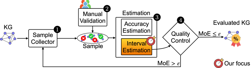
Figure 1. Efficient KG accuracy evaluation framework (Marchesin and Silvello, 2024).

In phase , a small batch of triples is drawn from the KG according to a chosen sampling strategy $\mathcal{S}$. This strategy should be selected to minimize the cost function, representing the optimization objective. In phase , manual annotations are obtained for these newly sampled triples and combined with any existing annotations. In phase , using the annotations accumulated via the chosen sampling design, an unbiased estimator computes $\hat{\mu}$, the estimate of the KG accuracy. The annotated sample also constructs the corresponding $1-\alpha$ interval, quantifying the uncertainties in the sampling procedure. In phase , a quality control step checks whether the generated interval meets the predefined upper bound, ensuring that $\text{MoE}\leq\varepsilon$. If the criterion is satisfied, the process concludes, and the accuracy estimate and the corresponding $1-\alpha$ interval are reported. If not, the process returns to phase . Thus, the framework iteratively samples and estimates, stopping when the interval meets the specified threshold $\varepsilon$. Doing so avoids oversampling and unnecessary manual annotations, ensuring accurate and cost-effective estimates.

The fact that the problem is solved once the interval is sufficiently narrow highlights the pivotal role of $\mathbf{1-\alpha}$ intervals in the optimization process. Given a sampling strategy, faster-shrinking intervals allow the problem to be solved with smaller samples, thereby reducing the number of required annotations compared to other, slower-to-converge intervals. At the same time, it is also essential that $1-\alpha$ intervals are reliable and guarantees the statistical properties they (nominally) entail, as first outlined in (Marchesin and Silvello, 2024). However, to ensure reliability in the evaluation process, the approach by Marchesin and Silvello (2024) required a trade-off, thus sacrificing some efficiency. In this work, by shifting the interval estimation framework from frequentist to Bayesian statistics, we demonstrate that it is possible to obtain intervals that are guaranteed to be the shortest – and thus the most efficient – while also providing probabilistic solid guarantees on their reliability.

2.4. Sampling and Accuracy Estimation

The approaches proposed to efficiently evaluate KG accuracy (Gao et al., 2019; Qi et al., 2022; Marchesin and Silvello, 2024) adopt simple and cluster random sampling techniques, paired with well-known point estimators (Cochran, 1977). Below, we detail both sampling strategies and the corresponding unbiased estimators.

Simple Random Sampling

Simple Random Sampling (SRS) draws a sample of $n_{\mathcal{S}}$ triples from $G$ without replacement. In large-scale KGs, the probability of choosing the same triple more than once is low, making sampling with replacement a good approximation to sampling without replacement (Casella and Berger, 2002) and a practical solution.

Under SRS, the estimator for $\mu$ is the sample proportion:

(2) $$\hat{\mu}_{\text{\scriptsize SRS}}=\frac{\sum_{i=1}^{n_{\mathcal{S}}}\mathds{1}(t_{i})}{n_{\mathcal{S}}}=\frac{\tau_{\mathcal{S}}}{n_{\mathcal{S}}}$$

with estimation variance given by $V(\hat{\mu}_{\text{\scriptsize SRS}})=\frac{\hat{\mu}_{\text{\scriptsize SRS}}(1-\hat{\mu}_{\text{\scriptsize SRS}})}{n_{\mathcal{S}}}$.

When SRS is applied, $\hat{\mu}_{\text{\scriptsize SRS}}$ is an unbiased estimator of $\mu$ (Cochran, 1977).

Cluster Random Sampling

Cluster sampling is a cost-effective alternative to SRS when estimating the accuracy of large-scale KGs (Gao et al., 2019; Qi et al., 2022; Marchesin and Silvello, 2024). Among the different cluster sampling strategies that can be employed, Two-stage Weighted Cluster Sampling (TWCS) represents the state-of-the-art for KG accuracy evaluation (Gao et al., 2019; Marchesin and Silvello, 2024). TWCS is divided into two stages. In the first stage, TWCS samples $n_{C}$ entity clusters with probabilities $\pi_{i}$ proportional to their sizes. That is, by denoting the size of the $i$th entity cluster as $M_{i}=|C_{e_{i}}|$, the cluster selection probability can be defined as $\pi_{i}=M_{i}/M$. In the second stage, TWCS draws $\min\{M_{i},m\}$ triples from each sampled cluster using SRS without replacement.

Let $\hat{\mu}_{i}$ be the (estimated) accuracy of the $i$th entity cluster. The estimator for $\mu$ under TWCS is:

(3) $$\hat{\mu}_{\text{\scriptsize TWCS}}=\frac{\sum_{i=1}^{n_{C}}\hat{\mu}_{i}}{n_{C}}$$

with estimation variance $V(\hat{\mu}_{\text{\scriptsize TWCS}})=\frac{1}{n_{C}(n_{C}-1)}\sum_{i=1}^{n_{C}}(\hat{\mu}_{i}-\hat{\mu}_{\text{\scriptsize TWCS}})^{2}$.

When TWCS is applied with a second-stage sample of approximately size $m$, $\hat{\mu}_{\text{\scriptsize TWCS}}$ is an unbiased estimator of $\mu$ (Cochran, 1977).

3. State of the Art: Confidence Intervals (CIs)

Previous research on efficient KG accuracy evaluation has utilized CIs to estimate $1-\alpha$ intervals (Gao et al., 2019; Qi et al., 2022; Marchesin and Silvello, 2024). However, no universal formula exists for constructing CIs under arbitrary sampling strategies (and point estimators). Instead, multiple approaches have been developed (Brown et al., 2001), each offering CIs with distinct properties (Morey et al., 2016). Among these, we review only the methods employed by state-of-the-art KG accuracy estimation techniques — specifically, the Wald and Wilson approaches (Casella and Berger, 2002; Wilson, 1927).

This section outlines Wald and Wilson methods for constructing $1-\alpha$ CIs. Next, we discuss the common misinterpretations and the resulting fallacies regarding CIs concerning their confidence, precision, and likelihood properties (Morey et al., 2016), which are desirable characteristics for tasks where analysts seek reasonable post-data inference, such as in KG accuracy estimation.

3.1. The Wald Method

The Wald method relies on normal approximation to build $1-\alpha$ CIs and involves inverting the acceptance region of the Wald large-sample normal test (Casella and Berger, 2002):

(4) $$\left|\frac{\hat{\mu}_{\mathcal{S}}-\mu}{\sqrt{V(\hat{\mu}_{\mathcal{S}})}}\right|\leq z_{\alpha/2}$$

where $\mu$ represents the true KG accuracy, $\hat{\mu}_{\mathcal{S}}$ and $V(\hat{\mu}_{\mathcal{S}})$ the estimated KG accuracy and its variance under a given sampling strategy $\mathcal{S}$, and $z_{\alpha/2}$ the critical value of the standard normal distribution for a confidence level $1-\alpha$.

By solving Equation (4) in $\mu$, we obtain the $1-\alpha$ Wald interval:

(5) $$\hat{\mu}_{\mathcal{S}}\pm z_{\alpha/2}\sqrt{V(\hat{\mu}_{\mathcal{S}})}$$

The Wald interval is an appealing CI due to its simplicity. However, when applied to binomial proportions, it is known to incur overshooting and zero-width intervals (Brown et al., 2001), also presenting an erratic behavior when used to gauge KG accuracy (Marchesin and Silvello, 2024). These phenomena aggravate in KGs with accuracy values deviating from the center of the (accuracy) range – where normal approximation works best – towards its boundaries, that is, one or zero. Since many real-life KGs, such as YAGO, DBpedia, and Wikidata, involve a certain degree of manual curation, they rarely have accuracy values as low as $0.5$. Conversely, fully automated KGs, which are noisier and more error-prone, frequently present accuracy values well below $0.5$ (Pujara et al., 2017). Thus, this tendency of real-life KGs towards the boundaries of the accuracy range makes Wald an often unreliable choice for KG accuracy estimation.

3.2. The Wilson Method

To overcome Wald limitations, Marchesin and Silvello (2024) relied on the Wilson method (Wilson, 1927), which can be used to build $1-\alpha$ binomial CIs. Similarly to Wald, the method involves inverting the acceptance region of the significance test in Equation 4, but requires two changes. First, it requires assuming that the sampling strategy used to collect the sample is SRS. Secondly, it requires replacing the estimated standard error with the null standard error. Based on these changes, the test can thus be rewritten as:

(6) $$\left|\sqrt{\frac{n_{\mathcal{S}}}{\mu(1-\mu)}}\cdot(\hat{\mu}_{\text{\scriptsize SRS}}-\mu)\right|\leq z_{\alpha/2}$$

By solving Equation (6) in $\mu$, we get the $1-\alpha$ Wilson interval:

(7) $$\frac{\hat{\mu}_{\text{\scriptsize SRS}}+\frac{z_{\alpha/2}^{2}}{2n_{\mathcal{S}}}}{1+\frac{z_{\alpha/2}^{2}}{n_{\mathcal{S}}}}\pm\frac{z_{\alpha/2}}{1+\frac{z_{\alpha/2}^{2}}{n_{\mathcal{S}}}}\cdot\sqrt{\frac{\hat{\mu}_{\text{\scriptsize SRS}}(1-\hat{\mu}_{\text{\scriptsize SRS}})}{n_{\mathcal{S}}}+\frac{z_{\alpha/2}^{2}}{4n_{\mathcal{S}}^{2}}}$$

which, compared to the Wald interval, consists of a relocated center estimate (left) and a corrected standard deviation (right).

Wilson intervals correct the erratic behavior of Wald ones, resulting in higher reliability, although at the expense of a drop in efficiency as accuracy approaches its boundaries (Marchesin and Silvello, 2024). Note that design effect adjustments are also required to adapt Wilson to complex sampling strategies (Kish, 1965, 1995).

3.3. Confidence Intervals (CIs) Limitations

CIs fall under frequentist statistics, where probability is interpreted as the long-term frequency of events across repeated sampling. This means that, when building a CI, we are not directly estimating the probability that the parameter of interest – the KG accuracy in our case – lies within the interval. Instead, we estimate how frequently such intervals, across repeated trials, will catch the true parameter. This is often referred to as frequency probability.

Hence, CIs interpretation can be counterintuitive and, for this reason, is often misunderstood by practitioners (Hoekstra et al., 2014). Three major fallacies exist in interpreting CIs, as shown by  Morey et al. (2016). Although these fallacies do not affect the quantitative outcomes of KG accuracy evaluation, they pose a significant risk to the proper use of CIs. Misinterpretations stemming from them can lead to conclusions as flawed as those caused by quantitative inaccuracies. In the following, we first outline these fallacies and then provide a practical example where they occur.

Fallacy 1.

The probability that a $1-\alpha$ CI contains the true parameter is $1-\alpha$ for a particular observed interval.

This is a fallacious interpretation because once a CI is constructed, the probability that it contains the true parameter is either 1 (if it does) or 0 (if it does not). The $1-\alpha$ confidence level represents the reliability of the interval estimation procedure across repeated samples rather than the probability that any specific interval captures the true parameter. This misconception stems from the belief that a $1-\alpha$ CI provides the likelihood that the unknown parameter falls within the observed interval (Hoekstra et al., 2014). However, the $1-\alpha$ confidence level does not assess whether the specific interval computed from the data includes the true parameter. CIs rely on pre-data assumptions not intended for post-data inference (Neyman and Jeffreys, 1937).

Fallacy 2.

The width of a CI reflects the precision of our knowledge about the parameter.

This interpretation is flawed because there is no inherent relationship between the width of a CI and the precision of the parameter estimate. The $1-\alpha$ confidence level reflects the reliability of the interval estimation procedure, not the precision of a particular observed interval. Hence, it is impossible to know whether a specific narrow or wide interval belongs to the $1-\alpha$ proportion that reliably captures the true parameter or the $\alpha$ proportion that does not. Consequently, interpreting CI width as a measure of precision can lead to incorrect post-data conclusions (Morey et al., 2016).

Fallacy 3.

A CI includes the likely values of the parameter.

While a CI is constructed to have a fixed $1-\alpha$ probability of capturing the true parameter across repeated samples, this does not imply that any particular observed interval contains the most likely values for the parameter. Once the interval is calculated, it either includes the true parameter or does not (Neyman, 1941). Indeed, CIs can sometimes exclude many reasonable values or, in extreme cases, be infinitesimally narrow or even empty (e.g., Wald intervals (Brown et al., 2001)), thereby excluding all possible values (Morey et al., 2016).

Example 0.

Let us consider an analyst who wants to estimate the accuracy of NELL ($\mu=0.91$, see Table 1) using the evaluation framework described in Section 2.3. The analyst adopts the most straightforward approach with SRS for sampling, the Wald method with a significance level $\alpha=0.05$ for interval estimation, and a MoE threshold of $\varepsilon=0.05$ for convergence. Under this setup, the evaluation procedure halts (i.e., MoE $\leq\varepsilon$) with a sample size of $n_{\mathcal{S}}=30$ and an estimated accuracy of $\hat{\mu}_{\text{\scriptsize SRS}}=1.00$ – reasonable outcomes given the underlying KG accuracy. With these values, the estimation variance is $V(\hat{\mu}_{\text{\scriptsize SRS}})=0.00$. Substituting this into Equation (5) produces a zero-width interval: $\text{CI}=[1.00,1.00]$, meaning that there is an absolute certainty that the estimated accuracy $\hat{\mu}_{\text{\scriptsize SRS}}$ is correct. However, this also implies that the probability that the obtained CI contains the true accuracy cannot be $1-\alpha$. Therefore, placing $1-\alpha$ confidence in an interval that assumes absolute certainty would clearly be a mistake for the analyst (Fallacy 1). At the same time, a zero-width CI does not imply that effect size is determined with perfect precision, as that would require annotating the entire population, nor can it imply that there is a $0.95$ ($1-\alpha$) probability that $\mu$ is exactly $1.00$, thus leading to Fallacy 2. Finally, a zero-width interval excludes all the possible values the accuracy can take, resulting in Fallacy 3. Hence, these fallacies highlight that the post-data properties required to make valid inferences from the interval are absent, potentially leading to arbitrary conclusions.

Task-Specific Deterrents

The frequentist assumption underlying CIs – and the corresponding interpretation fallacies this can generate – makes these intervals not ideal for KG accuracy evaluation. In fact, CIs offer guarantees over repeated trials rather than for a specific instance. However, in real-life scenarios, KG accuracy evaluation is typically conducted as a single, non-repeated process. Hence, CIs are inconvenient and $1-\alpha$ intervals providing a reliable interpretation in a one-shot setting are very much desired.

Moreover, the lack of a unified framework for constructing CIs contributes to their complexity. Different CIs are generated using distinct construction methods, often relying on intricate procedures that involve assumptions and approximations that are rarely tested (Makowski et al., 2019). Additionally, CIs constructed through different methods can vary in efficiency and reliability across different regions of the accuracy space (Marchesin and Silvello, 2024). Therefore, establishing a unified framework that enables the seamless computation of multiple $1-\alpha$ intervals would be crucial for improving consistency and comparability.

Finally, the long-term properties of CIs necessitate additional metrics to assess their reliability, such as coverage probability (Marchesin and Silvello, 2024). However, calculating this probability requires repeated iterations of the entire KG accuracy evaluation procedure, making it impractical for real-world applications.

4. Proposed Solution: Credible Intervals (CrIs)

To overcome the limitations of CIs for KG accuracy evaluation, we can resort to Credible Intervals (CrIs) (Edwards et al., 1963). These intervals are grounded in Bayesian statistics and operate on the principle that estimated parameters are random variables following a distribution.

Bayesian statistics differs from the frequentist approach as it is a post-data theory (Morey et al., 2016). It uses the information from the data, combined with model assumptions and prior information, to determine what is reasonable to believe (Gelman, 2008; Wasserman, 2008).

In the Bayesian framework, probability represents a degree of belief in an event, captured by a distribution. Before observing data, this belief is expressed through a prior distribution, reflecting initial assumptions or knowledge about the parameter of interest. For instance, when estimating KG accuracy, the prior distribution encodes beliefs about likely accuracy values based on prior knowledge or judgment. Once data is collected, this initial belief is updated through the likelihood, representing the posterior probability – the focus of Bayesian statistics – from the observed data. This probability is obtained by conditioning the prior probability with the information summarized by the likelihood via Bayes’ rule (Box and Tiao, 2011).

A CrI is an interval derived from the posterior distribution, indicating the range within which an unobserved parameter value will likely fall with a certain probability. Since CrIs are defined on the posterior distribution, a $1-\alpha$ CrI has the following properties:

1. It contains the parameter of interest with $1-\alpha$ probability (addressing Fallacy 1).

2. Its width reflects the precision of the estimate (addressing Fallacy 2).

3. It covers the plausible values of the parameter (addressing Fallacy 3). Thus, Bayesian interval estimation avoids CIs interpretation fallacies by providing $1-\alpha$, interpretable and reliable intervals in a one-shot setting.

We introduce two families of CrIs: ET and HPD intervals (Box and Tiao, 2011). We demonstrate that HPD intervals are the shortest possible, providing the best representation of parameter values most consistent with the data. Additionally, we show that ET and HPD intervals are equivalent when the posterior distribution is symmetric. Finally, we address the challenges of selecting an appropriate prior by proposing a new adaptive solution that eliminates the need for manual prior selection while ensuring optimal performance.

4.1. Bayesian Interval Estimation

We model the process of annotating triples for correctness as a binomial process $\operatorname{Bin}(n_{\mathcal{S}},\mu)$, where $n_{\mathcal{S}}\geq 1$ is the number of annotated triples and $\mu$ represents the binomial proportion (cf. Eq. (1)). Since beta distributions are the standard conjugate priors for binomial distributions, using them for inference on $\mu$ is suitable (Berger, 1985).

Let $\tau_{\mathcal{S}}\sim\operatorname{Bin}(n_{\mathcal{S}},\mu)$, and assume that $\mu$ has a prior distribution $\operatorname{Beta}(a,b)$, where $a,b>0$ represent our prior belief regarding correct ($a$) and incorrect ($b$) triples in the KG. Due to the conjugate relationship between beta and binomial distributions, the posterior distribution of $\mu$ can be derived as $\operatorname{Beta}(a+\tau_{\mathcal{S}},b+n_{\mathcal{S}}-\tau_{\mathcal{S}})$ (Raiffa and Schlaifer, 1961). This means that to obtain the beta posterior, we simply update the parameters of the beta prior by adding the observed number of correct ($\tau_{\mathcal{S}}$) and incorrect ($n_{\mathcal{S}}-\tau_{\mathcal{S}}$) triples.

Let $F(\mu~|~G_{\mathcal{S}})$ denote the posterior Cumulative Distribution Function (CDF) of $\mu$. For a given $\alpha$, we can identify an interval $(l,u)$ such that:

(8) $$1-\alpha=\operatorname{Pr}(l\leq\mu\leq u~|~G_{\mathcal{S}})=F(u)-F(l)$$

Therefore, a $1-\alpha$ CrI is an interval $(l,u)$ that satisfies the condition $1-\alpha=F(u)-F(l)$ (Press, 2002). However,it remains to decide how to compute such an interval.

4.2. Equal-Tailed (ET) Intervals

A common solution is that of Equal-Tailed (ET) intervals (McElreath, 2020). These are $1-\alpha$ CrIs that allocate equal probability to the tails of the posterior distribution – i.e., below the lower bound $l$ and above the upper bound $u$. In other words, a $1-\alpha$ ET CrI is obtained by taking the central $1-\alpha$ region of the posterior distribution, leaving $\alpha/2$ probability in each tail. By denoting $\operatorname{qBeta}(i;\cdot,\cdot)$ as the $i$th quantile of a beta distribution, we define the $1-\alpha$ ET CrI as:

(9) $$\begin{split}&l=\operatorname{qBeta}(\alpha/2;a+\tau_{\mathcal{S}},b+n_{\mathcal{S}}-\tau_{\mathcal{S}})\\ &u=\operatorname{qBeta}(1-\alpha/2;a+\tau_{\mathcal{S}},b+n_{\mathcal{S}}-\tau_{\mathcal{S}})\end{split}$$

While ET CrIs are intuitive and effective for symmetric posteriors, they become suboptimal for skewed distributions because, by design, they allocate $\alpha/2$ of the distribution in each tail. To illustrate this, consider Figure 2, which shows three scenarios with increasing skewness in the posterior distribution for KG accuracy. In the symmetric case (Figure 2(a)), the ET CrI captures the most probable values (purple region), providing a good summary of the distribution. However, as skewness increases (Figures 2(b,c)), the ET CrI includes lower-probability parameter values (red region) while excluding parts of the HPD region (blue region). This results in a longer interval than necessary to satisfy the condition $1-\alpha=F(u)-F(l)$.

To further support this, we compared the CDF of the HPD region excluded by the ET CrI with the CDF of any equally wide region covered by ET but falling outside the HPD region. In the moderately skewed case (Figure  2(b)), the CDF of these regions falling outside the HPD region, but covered by the ET CrI, is always less than 75% of the CDF of the HPD region not covered by the ET CrI. In the highly skewed case (Figure 2(c)), the CDF of these non-HPD regions is not even the $20\%$ of the CDF of the excluded HPD region. We can see that, in both cases, the exclusion of portions of the HPD region forces the ET interval to expand in width to satisfy the $1-\alpha=F(u)-F(l)$ constraint, making it a suboptimal choice.

Moreover, for skewed posteriors, the inability of ET CrIs to fully cover the HPD region makes them vulnerable to Fallacy 3. Thus, for KG accuracy evaluation, where skewed distributions are common, ET limitations are of significance.

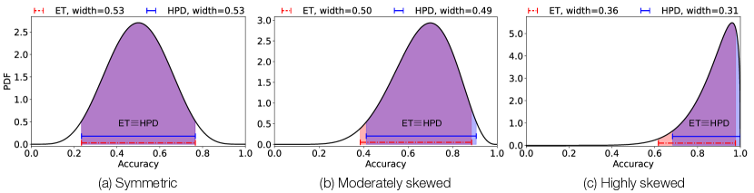
Figure 2. Comparison of ET and HPD CrIs across three posterior distributions for KG accuracy with increasing skewness (from left to right). In panel (a), where the posterior is symmetric, both ET and HPD intervals capture the most probable values (purple region). However, as skewness increases in panels (b) and (c), the ET interval deviates from the highest posterior density region, including less likely parameter values (red region), and resulting in unnecessarily longer intervals to satisfy the $1-\alpha=F(u)-F(l)$ condition. In contrast, the HPD intervals remain optimal, covering only the highest posterior density region (purple and blue regions), thereby highlighting the superior performance of HPD in skewed distributions compared to ET.

4.3. Highest Posterior Density (HPD) Intervals

The $1-\alpha$ CrI that best describes the posterior distribution is the interval containing the most probable posterior values (McElreath, 2020), i.e., the Highest Posterior Density (HPD) interval.

Definition.

Let $f(\mu|G_{\mathcal{S}})$ represent the Probability Density Function (PDF) of the posterior distribution. A $1-\alpha$ CrI is an HPD interval if it satisfies the following two conditions:

1. $F(u)-F(l)=1-\alpha$;

2. For $l\leq\mu\leq u$, $f(\mu|G_{\mathcal{S}})$ is greater than for any other interval where condition (1) holds.

The first condition corresponds to the general definition of a $1-\alpha$ CrI (see Eq. (8)), while the second ensures that every point inside the HPD interval has higher PDF value than points outside. Given these conditions, within the Bayesian framework designed in Section 4.1, the HPD interval is the smallest possible and unique. As we will see in Section 6, these properties translate into more cost-effective solutions for KG accuracy evaluation.

First, we prove both properties for the standard case, where the number of correct ($\tau_{\mathcal{S}}$) and incorrect ($n_{\mathcal{S}}-\tau_{\mathcal{S}}$) triples resulting from the annotation process are nonzero. Due to space limits, we report sketch proofs. The complete proofs are in the online repository.

Theorem 1.

Given a prior distribution $\operatorname{Beta}(a,b)$ for $\mu$ and a KG correctness annotation process, where $0<\tau_{\mathcal{S}}<n_{\mathcal{S}}$, the $1-\alpha$ HPD interval is the smallest $(l,u)$ interval satisfying the condition $F(u)-F(l)=1-\alpha$.

Sketch Proof.

When $0<\tau_{\mathcal{S}}<n_{\mathcal{S}}$, the beta posterior $\operatorname{Beta}(a+\tau_{\mathcal{S}},b+n_{\mathcal{S}}-\tau_{\mathcal{S}})$ is unimodal and continuous over $[0,1]$, ensuring the existence of a CrI. To find the smallest interval satisfying $F(u)-F(l)=1-\alpha$, we apply the method of Lagrange multipliers, which minimizes the interval length $(u-l)$ under the constraint that the posterior probability over $[l,u]$ equals $1-\alpha$. That is, we minimize the Lagrangian function $\mathcal{L}=(u-l)+\lambda\Bigl{(}\int_{l}^{u}f(\mu~|~G_{\mathcal{S}})~d\mu-(1-\alpha)\Bigr{)}$, where $\lambda$ is the Lagrange multiplier.

From the first-order conditions $\partial\mathcal{L}/\partial l=0$ and $\partial\mathcal{L}/\partial u=0$, we derive $f(l~|~G_{\mathcal{S}})=f(u~|~G_{\mathcal{S}})=-\frac{1}{\lambda}$. We compute the second-order derivatives to verify that $(l,u)$ minimizes $\mathcal{L}$. The unimodal nature of the posterior ensures that the derived Hessian matrix is positive definite, confirming that $(l,u)$ is the smallest interval satisfying $F(u)-F(l)=1-\alpha$. ∎

Theorem 2.

Under the assumptions of Theorem 1, the $1-\alpha$ HPD interval is unique.

Sketch Proof.

Let $(l^{*},u^{*})$ represent the HPD interval. Assume by contradiction that there exists another interval $(l^{\prime},u^{\prime})\neq(l^{*},u^{*})$ such that $(u^{\prime}-l^{\prime})=(u^{*}-l^{*})$ and $\int_{l^{\prime}}^{u^{\prime}}f(\mu~|~G_{\mathcal{S}})~d\mu=1-\alpha$. Since the posterior is unimodal, Th. 1 ensures that the HPD interval contains the mode. Similarly, the alternative interval $(l^{\prime},u^{\prime})$ must also contain the mode. Hence, given that $(l^{\prime},u^{\prime})\neq(l^{*},u^{*})$ but $(u^{\prime}-l^{\prime})=(u^{*}-l^{*})$, two cases arise: (i) $l^{\prime}<l^{*}$ and $u^{\prime}<u^{*}$; or (ii) $l^{\prime}>l^{*}$ and $u^{\prime}>u^{*}$. We prove case (i); case (ii) is analogous.

Since both intervals satisfy the condition $F(u)-F(l)=1-\alpha$, then it must hold that $\int_{l^{\prime}}^{u^{\prime}}f(\mu~|~G_{\mathcal{S}})~d\mu$ $=\int_{l^{*}}^{u^{*}}f(\mu~|~G_{\mathcal{S}})~d\mu$. Removing the common terms yields: $\int_{l^{\prime}}^{l^{*}}f(\mu~|~G_{\mathcal{S}})~d\mu=\int_{u^{\prime}}^{u^{*}}f(\mu~|~G_{\mathcal{S}})~d\mu$. However, since $l^{\prime}$ lies outside the HPD region while $u^{\prime}$ lies inside, it follows that $\int_{l^{\prime}}^{l^{*}}f(\mu~|~G_{\mathcal{S}})~d\mu<\int_{u^{\prime}}^{u^{*}}f(\mu~|~G_{\mathcal{S}})~d\mu$, which contradicts the equality assumption. ∎

To compute the $1-\alpha$ HPD CrI, we need to find the $(l,u)$ interval that minimizes the Lagrangian function $\mathcal{L}$ defined in Th. 1. We resort to sequential quadratic programming by adopting the Sequential Least SQuares Programming (SLSQP) optimizer (Kraft, 1988), that minimizes a Lagrangian of several variables with any combination of bounds, equality, and inequality constraints. SLSQP reformulates the optimization problem into a sequence of quadratic subproblems whose objectives are second-order approximations of the original Lagrangian and whose constraints are linearized versions of the original ones. The method then applies globalization techniques to guarantee convergence.

In our case, the objective of the Lagrangian is minimizing the $(l,u)$ interval width, with $l$ and $u$ bounded to the $[0,1]$ probability domain. The enforced (equality) constraint is $\int_{l}^{u}f(\mu~|~G_{\mathcal{S}})~d\mu=1-\alpha$. To accelerate convergence, we use the corresponding $1-\alpha$ ET CrI as an initial guess for the SLSQP optimizer.

Limiting Cases.

The minimality and uniqueness properties of the $1-\alpha$ HPD interval can be extended to limiting cases where the beta posterior exhibits exponentially increasing or decreasing behavior. These cases arise when the beta prior is uninformative – i.e., $a\!=\!b\leq 1$ – and the annotation process yields either all correct ($\tau_{\mathcal{S}}=n_{\mathcal{S}}$) or all incorrect ($\tau_{\mathcal{S}}=0$) triples.

When $\tau_{\mathcal{S}}=n_{\mathcal{S}}$, resulting in an exponentially increasing posterior, the $1-\alpha$ HPD interval is computed as:

(10) $$l=\operatorname{qBeta}(\alpha;a+\tau_{\mathcal{S}},b);~u=1$$

Likewise, when $\tau_{\mathcal{S}}=0$, producing an exponentially decreasing posterior, the $1-\alpha$ HPD interval becomes:

(11) $$l=0;~u=\operatorname{qBeta}(1-\alpha;a,b+n_{\mathcal{S}})$$

As a corollary to Theorem 1, we prove that the $1-\alpha$ HPD interval is minimal in both limiting cases.

Corollary 0.

Given an uninformative $\operatorname{Beta}(a,b)$ prior for $\mu$ and a KG annotation process resulting in either all correct ($\tau_{\mathcal{S}}=n_{\mathcal{S}}$) or all incorrect ($\tau_{\mathcal{S}}=0$) triples, the $1-\alpha$ HPD interval is the smallest $(l,u)$ interval satisfying $F(u)-F(l)=1-\alpha$.

Proof.

We prove $\tau_{\mathcal{S}}=0$, the proof for $\tau_{\mathcal{S}}=n_{\mathcal{S}}$ is symmetrical. With an uninformative prior (i.e., $a=b\leq 1$) and an annotation outcome $\tau_{\mathcal{S}}=0$, the resulting beta posterior has parameters $a\leq 1$ and $b+n_{\mathcal{S}}>1$, exhibiting an exponentially decreasing behavior with the highest density in $x=0$. Due to the monotonicity of the beta posterior, for any $x_{1}<x_{2}$, we have $f(x_{1}~|~G_{\mathcal{S}})>f(x_{2}~|~G_{\mathcal{S}})$. Thus, the HPD interval, with a lower bound at $0$ and an upper bound at the $1-\alpha$ quantile, is by construction the shortest interval containing $\mu$ with probability $1-\alpha$. ∎

Similarly, we prove its uniqueness as a corollary to Theorem 2.

Corollary 0.

Under the assumptions of Corollary 3, the $1-\alpha$ HPD interval is unique.

Sketch Proof.

The proof follows the same rationale as the proof of Theorem 2. We prove for both limiting cases – $\tau_{\mathcal{S}}=0$ and $\tau_{\mathcal{S}}=n_{\mathcal{S}}$ – by contradiction. Suppose another interval $(l^{\prime},u^{\prime})$ exists with the same properties as the $1-\alpha$ HPD interval. This interval could either overlap with the HPD or lie entirely outside its range. In the overlapping case, the proof mirrors that of Theorem 2. For the external case, due to the monotonicity of the posterior distribution, it is trivial to show that the $(l^{\prime},u^{\prime})$ interval cannot have the same width as the HPD while covering $\mu$ with probability $1-\alpha$, thus proving the uniqueness of the HPD interval. ∎

Posterior Skewness.

The properties of $1-\alpha$ HPD CrIs make them suited for representing skewed posterior distributions. To verify this, we revisit Figure 2 with a focus on HPD intervals. When the distribution is skewed, as shown in Figures 2(b,c), the $1-\alpha$ HPD interval exhibits two expected properties. First, it is smaller than the corresponding $1-\alpha$ ET interval. Secondly, it only covers the most probable parameter values, resulting in a shift compared to the ET interval. Thus, for skewed posteriors, HPD CrIs provide the most precise and reliable summaries for post-data inference.

On the other hand, when the posterior is unimodal and symmetric, as in Figure 2(a), the HPD interval coincides with the ET interval. This relationship is formalized in the following theorem.

Theorem 5.

When the beta posterior for $\mu$ is unimodal and symmetric, the $1-\alpha$ HPD interval is equivalent to the $1-\alpha$ ET interval.

Sketch Proof.

Let $\omega$ represent the mode of a unimodal and symmetric posterior. By the symmetry property, for any $\delta>0$, we have $f(\omega-\delta~|~G_{\mathcal{S}})=f(\omega+\delta~|~G_{\mathcal{S}})$. Therefore, the $1-\alpha$ HPD interval is symmetric around $\omega$ – i.e., the lower and upper bounds, $l$ and $u$, are equidistant from $\omega$. Consequently, it follows that $\int_{0}^{l}f(\mu~|~G_{\mathcal{S}})~d\mu=\int_{u}^{1}f(\mu~|~G_{\mathcal{S}})~d\mu=\frac{\alpha}{2}$, which correspond to the CDFs of the $\alpha/2$ and $1-\alpha/2$ quantiles, respectively. That is, the $1-\alpha$ HPD and ET intervals coincide. ∎

This scenario occurs when, given a $\operatorname{Beta}(a,b)$ prior, the annotation process yields a $\operatorname{Beta}(a+\tau_{\mathcal{S}},b+n_{\mathcal{S}}-\tau_{\mathcal{S}})$ posterior where $a+\tau_{\mathcal{S}}=b+n_{\mathcal{S}}-\tau_{\mathcal{S}}$, which implies a post-data balance between correct and incorrect triples and hence a KG accuracy of $0.5$.

Implications

These theoretical results encompass all the scenarios that can be encountered in the annotation process for evaluating KG accuracy. These results stem from modeling the task, for the first time, through a beta-binomial process and account for configurations involving informative and uninformative priors. This led to new proofs tailored to the specific requirements of the considered task.

These findings have notable implications for data quality management because they show that HPD CrIs consistently optimize the convergence rate of the KG accuracy minimization problem across all possible scenarios. This translates into minimizing the number of annotations required to audit KG accuracy, thereby reducing temporal and monetary costs that are critical factors for data curation (Paulheim, 2018).

Furthermore, these theoretical insights extend beyond KG accuracy evaluation to any task involving a similar annotation process. As such, they hold broader applicability and significance, offering valuable contributions also to related domains.

4.4. The Challenge of Choosing the Right Prior

The Bayesian framework we designed for KG accuracy evaluation offers a seamless approach to build an infinite number of $1-\alpha$ CrIs by varying the $a,b$ parameters of the beta prior. This contrasts with frequentist methods, which involve different and complex procedures to generate $1-\alpha$ CIs that are challenging to interpret (Makowski et al., 2019; Morey et al., 2016). However, adopting the unified and flexible Bayesian approach requires choosing appropriate priors that optimize efficiency while ensuring reliability.

We focus on the most general and challenging scenario, where no prior knowledge or belief about the KG accuracy is available. In this case, using informative (or subjective) priors can be detrimental, leading to deceptive interpretations or inefficient solutions (Lesaffre and Lawson, 2012). To mitigate the bias introduced by these priors, we can resort to uninformative (or objective) priors (Press, 2002), which reflect a lack of available information about the underlying process. In other words, uninformative priors do not encode the analyst’s particular belief (or bias), making them suited to provide an objective analytical foundation. This allows the framework to be used by anyone – layman or expert – regardless of their specific expectations about the outcomes of the KG evaluation process.

For beta distributions, uninformative priors are characterized by parameters $a=b\leq 1$. In the literature, three proper (i.e., $a,b>0$) uninformative beta priors are widely used: Kerman $\operatorname{Beta}(\frac{1}{3},\frac{1}{3})$ (Kerman, 2011), Jeffreys $\operatorname{Beta}(\frac{1}{2},\frac{1}{2})$ (Jeffreys, 1946), and Uniform $\operatorname{Beta}(1,1)$ (Bayes, 1763). The Jeffreys prior is commonly adopted as the default choice for binomial proportion problems (Brown et al., 2001). However, it represents a trade-off between Kerman and Uniform priors (Jin et al., 2017), and as a result, it is never the most efficient option.

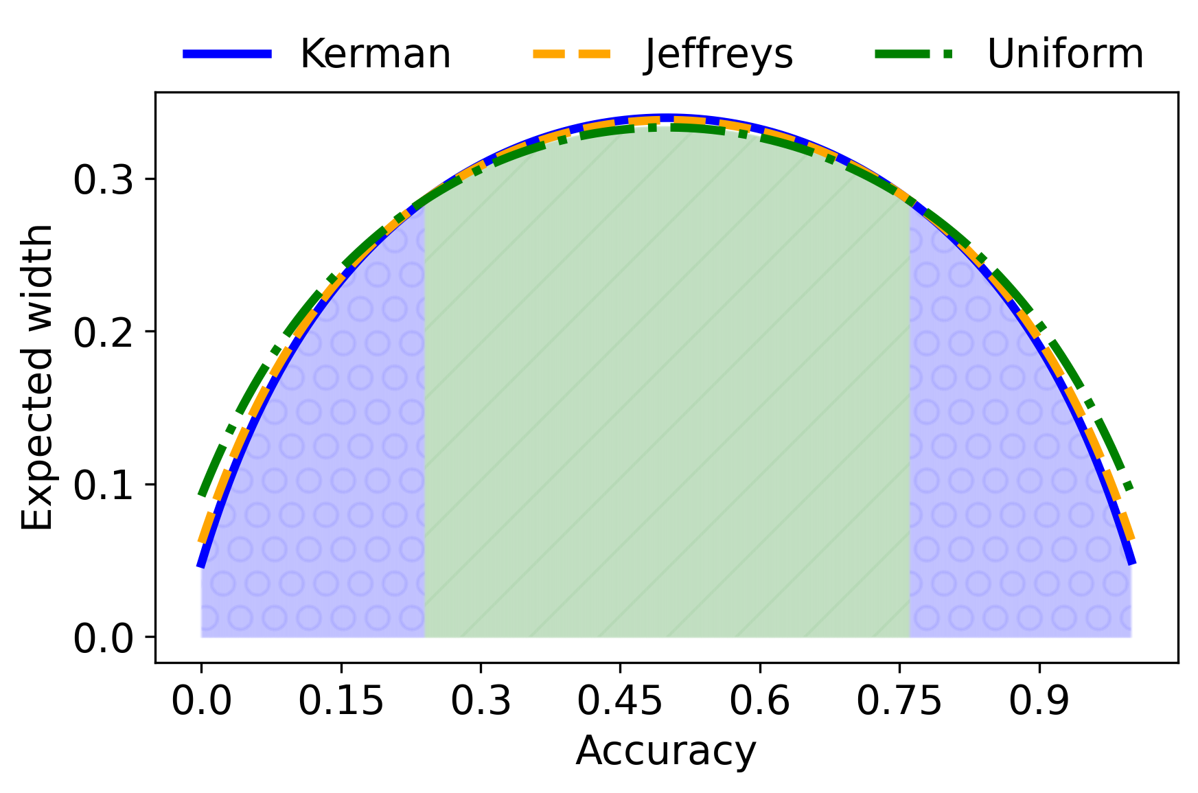
Figure 3. Expected width of HPD credible intervals under Kerman, Jeffreys, and Uniform priors for $n_{\mathcal{S}}=30$ and $\alpha=0.05$. The circle pattern ($\circ$) under the curves represents the set of accuracy values where Kerman prior provides the shortest expected width, whereas the line pattern ($//$) the set of accuracy values where Uniform performs best.

As an example, Figure 3 presents the expected width of $1-\alpha$ HPD intervals under Kerman, Jeffreys, and Uniform priors for $n_{\mathcal{S}}=30$ and $\alpha=0.05$. We can see that the HPD interval based on Jeffreys prior is never the shortest of the three. In contrast, Kerman- and Uniform-based HPD intervals achieve minimal widths depending on the specific accuracy space regions. Kerman-based intervals are optimal in the extreme regions, while Uniform-based intervals are optimal in the central region.

Despite being minor, these differences in interval widths lead to appreciable variations in annotation costs for KG accuracy evaluation. As we will see experimentally in Section 6.2, the annotation costs obtained under different priors are statistically different in most cases. This further underscores the importance of addressing the prior selection problem.

Therefore, choosing the right uninformative prior is a nontrivial decision. Since the outcome of the annotation process – and thus the region of the accuracy space where the estimate will fall – cannot be known in advance, it is impossible to choose, a priori, one prior that consistently optimizes efficiency.

4.5. The adaptive HPD (aHPD) algorithm

To address the challenge of prior selection, we propose the adaptive HPD (aHPD) algorithm (see Algorithm 1), where multiple uninformative priors are concurrently employed to generate distinct $1-\alpha$ HPD intervals.

Algorithm 1 adaptive HPD

1:

2:The KG $G$;

3:The significance level $\alpha$;

4:The sampling strategy $\mathcal{S}$;

5:The upper bound $\varepsilon$ for the MoE;

6:The set of uninformative beta prior parameters $\{(a_{1},b_{1}),\ldots,(a_{k},b_{k})\}$;

7:The estimated accuracy and the smallest $1-\alpha$ HPD interval.

8:Define objective function (obj) to minimize interval width $(u-l)$

9:Define constraint function (constr) to satisfy $F(u)-F(l)=1-\alpha$

10:$\texttt{bounds}\leftarrow[[0,1],[0,1]]$ $\triangleright$ Set $l$ and $u$ bounds

11:$\texttt{mu}\leftarrow 0$, $\texttt{moe}\leftarrow 1$, $\texttt{sample}\leftarrow\emptyset$ $\triangleright$ Initialization

12:while $\texttt{moe}>\varepsilon$ do

13:  $\texttt{batch}\leftarrow\mathcal{S}(G)$ $\triangleright$ Sample batch of facts from $G$ via $\mathcal{S}$

14:  $\texttt{annot}\leftarrow\mathds{1}(\texttt{batch})$ $\triangleright$ Annotate batch and store annotations

15:  $\texttt{sample}\leftarrow\texttt{sample}\cup\texttt{annot}$ $\triangleright$ Update sample with new annotations

16:  $\texttt{mu}\leftarrow\hat{\mu}_{\mathcal{S}}(\texttt{sample})$ $\triangleright$ Estimate $G$ accuracy from sample

17:  $\texttt{tau}\leftarrow\operatorname{sum}(\texttt{annot})$, $\texttt{n}\leftarrow|\texttt{sample}|$ $\triangleright$ Correct triples and sample size

18:  if $\mathcal{S}\;!\!=\,\text{SRS}$ then $\triangleright$ Complex sampling strategy

19:   Adjust for complex sampling effects using design effect corrections (Kish, 1995; Marchesin and Silvello, 2024)

20:  end if

21:  Compute posterior parameters from each prior and given annotation outcome:

22:$\;\;\;\;\;(\texttt{a\_post}_{i},\texttt{b\_post}_{i})\leftarrow(a_{i}+\texttt{tau},b_{i}+\texttt{n}-\texttt{tau})$

23:  if $\texttt{tau}==\texttt{n}$ then $\triangleright$ Limiting case (1): all facts correct

24:   $\texttt{l}_{i}\leftarrow\operatorname{qBeta}(\alpha;\texttt{a\_post}_{i},\texttt{b\_post}_{i})$, $\texttt{u}_{i}\leftarrow 1\,\forall i\in\{1,\ldots,k\}$

25:  else if $\texttt{tau}==0$ then $\triangleright$ Limiting case (2): no correct facts

26:   $\texttt{l}_{i}\leftarrow 0$, $\texttt{u}_{i}\leftarrow\operatorname{qBeta}(1-\alpha;\texttt{a\_post}_{i},\texttt{b\_post}_{i})\,\forall i\in\{1,\ldots,k\}$

27:  else$\triangleright$ Standard case: unimodal posterior

28:   Compute, for each posterior, the $1-\alpha$ ET CrI as initial guess:

29:$\;\;\;\;\;\;\;\;\;\,\,\texttt{guess}_{i}\leftarrow\operatorname{ET}(1-\alpha;\texttt{a\_post}_{i},\texttt{b\_post}_{i})$

30:   Compute, for each posterior, the $1-\alpha$ HPD CrI using SLSQP optimizer:

31:$\;\;\;\;\;\;\;\;\;\,\,(\texttt{l}_{i},\texttt{u}_{i})\leftarrow\text{SLSQP}(\texttt{obj},\texttt{guess}_{i},\texttt{constr},\texttt{bounds})$

32:  end if

33:  $(\texttt{l},\texttt{u})\leftarrow\operatorname{arg\,min}_{i}(\texttt{u}_{i}-\texttt{l}_{i})$ $\triangleright$ Select smallest $1-\alpha$ HPD CrI

34:  $\texttt{moe}\leftarrow(\texttt{u}-\texttt{l})/2$ $\triangleright$ Update MoE

35:end while

36:return mu, $(\texttt{l},\texttt{u})$

At each stage of the KG evaluation process, the algorithm samples and annotates a batch of facts (lines 6-7), which combines with previous annotations to update the accuracy estimate (lines 8-9). Based on the number of correct facts and the sample size, aHPD first applies design effect adjustments in case of complex sampling strategies (Kish, 1995; Marchesin and Silvello, 2024) and then calculates the posterior parameters for each uninformative prior provided as input (lines 10-14); there is no limit to the number of priors that can be fed to the algorithm. It then builds the corresponding $1-\alpha$ HPD intervals. When the number of correct facts equals the sample size (lines 15-16), in the first limiting case, the posterior distribution takes an exponentially increasing shape, and the interval bounds are computed using Equation (10). When the number of correct facts is zero (lines 17-18), in the second limiting case, the posterior distribution follows an exponentially decreasing pattern, and the intervals are derived via Equation (11). For the standard case, having defined the objective function, constraints, and bounds (lines 1-3), the algorithm adopts the SLSQP optimizer to generate the $1-\alpha$ HPD intervals, using the corresponding ET intervals as initial guesses (lines 20-21). It selects the smallest one among the generated intervals and computes its MoE (lines 23-24). The process iterates until $\text{MoE}\leq\varepsilon$ (line 5), ensuring the selected $1-\alpha$ HPD interval meets the desired precision. Once the criterion is satisfied, the algorithm returns the estimated accuracy and the chosen interval. Note that the computation of posterior parameters (line 14) and the construction of $1-\alpha$ intervals (lines 16, 18, 20-21) can be parallelized for each input prior, ensuring that the algorithm remains efficient regardless of the number of considered priors.

The aHPD algorithm dynamically adjusts to the region of the accuracy space where the estimate lies after the annotation process. This adaptive approach ensures that the first interval achieving the desired precision halts the evaluation process, guaranteeing the most efficient outcome from the set of competing solutions.

aHPD with Informative Priors

Although in this work we focus on the most general and challenging scenario, where no prior knowledge or belief about the KG accuracy is available, if we have (reliable) prior knowledge, then aHPD can be seamlessly used with such informative priors to optimize performance further.

Example 0.

Let us assume that an analyst who wants to estimate the accuracy of DBpedia ($\mu=0.85$, see Table 1) already knows the accuracy of two similar KGs – which have accuracy values $\mu=0.80$ and $\mu=0.90$, respectively. Based on this knowledge, the analyst can set up two informative priors, e.g., ($a_{1}=80$, $b_{1}=20$) and ($a_{2}=90$, $b_{2}=10$), and plug them into aHPD. The performance obtained with these informative priors under TWCS, averaged over $1,000$ repetitions, are $63\pm 36$ triples and a cost of $0.72\pm 0.41$, instead of $222\pm 83$ triples and a cost of $2.55\pm 0.95$ when using aHPD equipped with Kerman, Jeffreys, and Uniform uninformative priors.

Hence, aHPD can lead to even more efficient solutions if prior knowledge is available. Meanwhile, poor informative priors can be detrimental, leading to deceptive interpretations or inefficient solutions. In these cases, relying on uninformative priors is better.

5. Experimental Setup

In the following, we report the considered datasets, the adopted cost function, the experimental configuration, and the evaluation procedure. We release data and code used in this work. Moreover, we provide more experimental results presenting additional sampling strategies in the online repository. While these results are consistent with those given in the main text, they are less critical and thus are made available online due to space limits.

Datasets

We consider data from various real-life KGs, whose statistics are reported in Table 1. Note that dataset sizes are rather small due to the manual labeling costs.

Table 1. Statistics for YAGO, NELL, DBPEDIA, FACTBENCH, and SYN 100M datasets.

	YAGO	NELL	DBPEDIA	FACTBENCH	SYN $100$M
Num. of facts	1,386	1,860	9,344	2,800	101,415,011
Num. of clusters	822	817	2,936	1,157	5,000,000
Avg. cluster size	1.69	2.28	3.18	2.42	20.28
Accuracy ($\mu$)	0.99	0.91	0.85	0.54	{0.9,0.5,0.1}

YAGO: a dataset sampled by Ojha and Talukdar (2017) from the YAGO2 KG (Hoffart et al., 2013), with facts referring to people, organizations, countries, and movies. The dataset was manually annotated by crowdsourcing workers, resulting in a ground-truth accuracy of $\mu=0.99$.

NELL: drawn by Ojha and Talukdar (2017) from the NELL KG (Mitchell et al., 2018), this dataset focuses on sports-related facts. It includes manual annotations by crowdsourcing workers for each fact, yielding a ground-truth accuracy of $\mu=0.91$.

DBPEDIA: a dataset sampled by Marchesin et al. (2024a) from DBpedia (Auer et al., 2007), covering a broad range of topics such as entertainment, news, history, sports, business, and science. Each fact in the dataset was manually annotated by at least three layman workers. The correctness label for every fact was then derived via quality-weighted majority voting, where (layman) worker quality was evaluated on an extra pool of facts supervised by expert workers. This annotation process resulted in a ground-truth accuracy of $\mu=0.85$.

FACTBENCH: a benchmark created by Gerber et al. (2015) to assess fact validation algorithms. It contains correct facts from DBpedia (Auer et al., 2007) and Freebase (Bollacker et al., 2007, 2008), and generates incorrect facts by modifying correct ones while adhering to domain and range constraints. We consider a configuration where incorrect facts are a mix produced using different negative example generation strategies, resulting in a ground-truth accuracy of $\mu=0.54$.

YAGO and NELL are the reference datasets used in the literature to evaluate KG accuracy estimation approaches (Ojha and Talukdar, 2017; Gao et al., 2019; Qi et al., 2022; Marchesin and Silvello, 2024). The DBPEDIA dataset is a proxy for one of the largest and widely used real-life KGs. Conversely, FACTBENCH represents a controlled scenario designed to assess the ability of automatic fact validation methods to distinguish between real (correct) and synthetic (incorrect) facts. Although unrealistic, FACTBENCH can be used to evaluate the behavior of KG accuracy estimation solutions in the quasi-symmetric case. Note that other datasets used by prior work exist, such as MOVIE (Gao et al., 2019) and OPIEC (Qi et al., 2022), but they are either not publicly (MOVIE) or only partially (OPIEC) available.

We assess the scalability of the methods by using SYN 100M (Marchesin and Silvello, 2024), a synthetic dataset with over $100$ million triples, where correctness labels are generated by setting the probability of a triple being true to a fixed rate. We consider ground-truth accuracy values of $\mu\in\{0.9,0.5,0.1\}$.

Annotation Cost

We use the cost function proposed by (Gao et al., 2019) and later adopted in (Qi et al., 2022; Marchesin and Silvello, 2024) to measure the manual effort required to assess the correctness of facts in a given sample. The function is based on the assumption that annotating a fact for an entity already identified incurs a lower cost than annotating a fact from an unseen entity. Specifically, it divides the annotation process into entity identification, which involves linking the entity to the corresponding real-world concept, and fact verification, which entails collecting evidence and auditing the fact stated by the triple.

The cost function is expressed as:

(12) $$\operatorname{cost}(G_{\mathcal{S}})=|E_{\mathcal{S}}|\cdot c_{1}+|T_{\mathcal{S}}|\cdot c_{2}$$

Here, $c_{1}$ and $c_{2}$ represent the average time cost (in seconds) for entity identification and fact verification, respectively. In line with prior research (Gao et al., 2019; Qi et al., 2022; Marchesin and Silvello, 2024), we set $c_{1}=45$ and $c_{2}=25$ (seconds).

Sampling Strategies

We adopt SRS and TWCS as sampling strategies (Section 2.4). Based on the recommendation by Gao et al. (2019) to choose the second-stage size $m$ of TWCS in the range $\{3,5\}$, we set $m=3$ for YAGO, NELL, DBPEDIA, and FACTBENCH, which have small clusters, and $m=5$ for SYN 100M, which presents larger clusters (see Table 1).

Interval Estimation

We consider Wald (Section 3.1) and Wilson (Section 3.2) CIs as baselines and compare them with the aHPD (Section 4.5). Wald represents an efficient yet unreliable baseline, which we consider only to emphasize the efficiency of our approach further. Conversely, Wilson represents the current state-of-the-art, providing a trade-off between efficiency and (frequentist) reliability. For aHPD, we employ three uninformative priors: Kerman $\operatorname{Beta}(\frac{1}{3},\frac{1}{3})$, Jeffreys $\operatorname{Beta}(\frac{1}{2},\frac{1}{2})$, and Uniform $\operatorname{Beta}(1,1)$. We also evaluate the performance of ET (Section 4.2) and HPD (Section 4.3) CrIs under these priors. We apply the design effect adjustments from (Marchesin and Silvello, 2024) when the considered intervals are used with TWCS.

Evaluation Procedure

We set the significance level at $\alpha\in\{0.10,0.05,0.01\}$ and define the upper bound for the MoE as $\varepsilon=0.05$. When not specified, the significance level defaults to $\alpha=0.05$. We use two metrics to compare methods: the number of annotated triples and the annotation cost (in hours). The number of triples represents a simple and plain measure, while the annotation cost reflects a more realistic measure of temporal (and monetary) costs.

Results are reported when $\text{MoE}\leq 0.05$, ensuring the methods are compared once they satisfy the optimization constraint. For this reason, we do not report the width of CIs, as all solutions have $\text{MoE}\leq 0.05$. Similarly, accuracy estimates are omitted since all methods provide unbiased estimates with minimal deviation from ground-truth accuracy (less than $0.02$).

To account for the inherent variability of sampling strategies, we repeat the evaluation procedure $1,000$ times per method, reporting the mean and standard deviation for both the number of triples and the annotation cost.

6. Experimental Results

The objectives of the experiments are to (1) assess the impact of prior selection on KG accuracy estimation methods; (2) evaluate the efficiency of the aHPD compared to the state-of-the-art; (3) test whether aHPD is still efficient with large-scale datasets; and, (4) verify the robustness of aHPD across different levels of precision.

6.1. Summary of the Experimental Findings

• There is no one-prior-fits-all solution. Section 6.2 shows that there is no single prior that we can apply to obtain top performance consistently, thus motivating the need for the aHPD.

• aHPD outperforms state-of-the-art solutions in all real-life cases. Section 6.3 shows that aHPD reduces convergence costs compared to Wald and Wilson in common cases with a skewed accuracy distribution.

• aHPD scales efficiently to large datasets. Section 6.4 shows that the dataset size does not affect the performance of aHPD, which remains the most efficient solution.

• aHPD is robust across varying levels of precision. Section 6.5 shows that aHPD preserves its optimal performance regardless of the precision level required by the evaluation process.

6.2. Prior Selection

The performance of ET and HPD CrIs under Kerman, Jeffreys, and Uniform priors are reported in Table 2, together with those of aHPD equipped with the three considered priors. For sampling, we resorted to SRS, which allows for a clean comparison between CrIs built from different priors without introducing clustering. Such effects can hamper the interpretation of the results, making it challenging to determine whether the observed outcomes are due to the specific prior under consideration or to clustering effects.

Table 2. Performance of ET and HPD CrIs on YAGO, NELL, DBPEDIA, and FACTBENCH under different priors using SRS. For each interval, the best performances are in bold. We also report the performance obtained by aHPD equipped with the considered priors.

		YAGO	NELL	DBPEDIA	FACTBENCH
		$\mu=0.99$	$\mu=0.91$	$\mu=0.85$	$\mu=0.54$
Interval	Prior	Triples	Triples	Triples	Triples
ET	Kerman	$\mathbf{38\!\pm\!6}$	$\mathbf{104\!\pm\!40}$	$\mathbf{187\!\pm\!36}$	$380\!\pm\!3$
	Jeffreys	$39\!\pm\!7$	$107\!\pm\!39$	$188\!\pm\!34$	$379\!\pm\!3$
	Uniform	$41\!\pm\!9$	$113\!\pm\!36$	$190\!\pm\!32$	$\mathbf{378\!\pm\!3}$
HPD	Kerman	$\mathbf{32\!\pm\!5}$	$\mathbf{96\!\pm\!44}$	$\mathbf{182\!\pm\!42}$	$380\!\pm\!3$
	Jeffreys	$33\!\pm\!6$	$99\!\pm\!42$	$184\!\pm\!39$	$379\!\pm\!3$
	Uniform	$34\!\pm\!9$	$106\!\pm\!40$	$187\!\pm\!36$	$\mathbf{378\!\pm\!3}$
aHPD	$\{$K, J, U$\}$	$\mathbf{32\!\pm\!5}$	$\mathbf{96\!\pm\!44}$	$\mathbf{182\!\pm\!42}$	$\mathbf{378\!\pm\!3}$

The results in Table 2 confirm that Kerman and Uniform priors lead to the most efficient solutions in the extreme and central regions of the accuracy space, respectively (cf. Section 4.4). Conversely, the Jeffreys prior never achieves top performance. This pattern holds for both ET and HPD CrIs, highlighting the generality of the problem of choosing an appropriate prior.

Focusing on HPD intervals, the annotation costs under different priors are statistically different in 8 out of 12 cases, as determined by standard independent t-tests with $p<0.01$. This emphasizes that the choice of the prior significantly affects the outcomes. In this regard, aHPD, which automatically selects the optimal prior (cf. Table 2), proves to be statistically better than HPD solutions relying on suboptimal priors in $75\%$ of cases. Therefore, aHPD emerges as a robust approach for consistently selecting the optimal prior for a given annotation process, removing the need to choose a priori.

It is worth noting that other priors could be explored, which may perform better than the considered three in specific regions of the accuracy space. This further stresses the problem of prior selection when optimizing efficiency. For this work, we focused on three of the most popular priors, showing that even with a relatively small set, it is impossible to guarantee optimal performance across the entire accuracy space without knowing where the accuracy estimate will fall after the annotation process. This strengthens the need for an adaptive solution as the aHPD.

As a side note, Table 2 also shows that HPD intervals are better than ET ones when the accuracy is skewed (YAGO, NELL, DBPEDIA) and equal when the accuracy is quasi-symmetric (FACTBENCH), as proved by Theorems 1-5.

6.3. Efficiency

The performance of aHPD against Wald and Wilson baselines is reported in Table 3. We compared methods considering both SRS and TWCS as sampling strategies. We also performed statistical analyses to assess the significance of the performance differences between aHPD and baselines. Specifically, we conducted standard independent t-tests between aHPD and Wald, and between aHPD and Wilson, reporting statistical results when $p<0.01$.

Table 3. Performance on YAGO, NELL, DBPEDIA, and FACTBENCH. For TWCS, we set $m=3$. For each sampling strategy, best performance are in bold. ^† denotes a statistically significant difference between aHPD and Wald, while ^‡ indicates a significant difference between aHPD and Wilson, as determined by standard independent t-tests with $p<0.01$.

		YAGO		NELL		DBPEDIA		FACTBENCH
		$\mu=0.99$		$\mu=0.91$		$\mu=0.85$		$\mu=0.54$
Sampling	Interval	Triples	Cost	Triples	Cost	Triples	Cost	Triples	Cost
SRS	Wald	$33\!\pm\!7$	$0.62\!\pm\!0.12$	$103\!\pm\!43$	$1.89\!\pm\!0.76$	$188\!\pm\!38$	$3.55\!\pm\!0.71$	$382\!\pm\!3$	$6.37\!\pm\!0.10$
	Wilson	$41\!\pm\!10$	$0.76\!\pm\!0.18$	$114\!\pm\!36$	$2.08\!\pm\!0.63$	$190\!\pm\!32$	$3.60\!\pm\!0.60$	$\mathbf{378\!\pm\!3}$	$\mathbf{6.32\!\pm\!0.10}$
	aHPD	$\mathbf{32\!\pm\!5}$	$\mathbf{0.60\!\pm\!0.09}^{\dagger,\ddagger}$	$\mathbf{96\!\pm\!44}$	$\mathbf{1.76\!\pm\!0.79}^{\dagger,\ddagger}$	$\mathbf{182\!\pm\!42}$	$\mathbf{3.45\!\pm\!0.78}^{\dagger,\ddagger}$	$\mathbf{378\!\pm\!3}$	$\mathbf{6.32\!\pm\!0.10}^{\dagger}$
TWCS	Wald	$32\!\pm\!4$	$0.42\!\pm\!0.05$	$126\!\pm\!70$	$1.58\!\pm\!0.87$	$243\!\pm\!75$	$2.80\!\pm\!0.87$	$\mathbf{254\!\pm\!37}$	$\mathbf{3.08\!\pm\!0.45}$
	Wilson	$35\!\pm\!4$	$0.47\!\pm\!0.06$	$129\!\pm\!67$	$1.62\!\pm\!0.84$	$234\!\pm\!73$	$2.69\!\pm\!0.84$	$257\!\pm\!39$	$3.11\!\pm\!0.48$
	aHPD	$\mathbf{31\!\pm\!2}$	$\mathbf{0.41\!\pm\!0.03}^{\dagger,\ddagger}$	$\mathbf{112\!\pm\!68}$	$\mathbf{1.40\!\pm\!0.85}^{\dagger,\ddagger}$	$\mathbf{222\!\pm\!83}$	$\mathbf{2.55\!\pm\!0.95}^{\dagger,\ddagger}$	$257\!\pm\!39$	$3.11\!\pm\!0.48$

Table 3 provides the following insights. aHPD statistically outperforms both Wald and Wilson methods across all datasets where the KG accuracy is skewed – i.e., YAGO, NELL, and DBPEDIA. This is a significant outcome, as it shows that aHPD surpasses not only the Wilson method, which sacrifices efficiency to ensure high (frequentist) reliability (Marchesin and Silvello, 2024) but also the unreliable, yet very efficient Wald method. Thus, aHPD, grounded in Bayesian statistics, provides interpretable and reliable results while improving efficiency.

For datasets with quasi-symmetric accuracy distributions, such as FACTBENCH, the performance of aHPD matches those of the Wilson method. This result is expected. Since FACTBENCH has an accuracy of $\mu=0.54$, we know that, among the considered priors, the Uniform one achieves optimal performance (see Table 2). We also know that, in this scenario, HPD and ET intervals are the same (Theorem 5). Then, since the Wilson CI can be seen as an approximation of the ET CrI based on the Uniform prior (Jin et al., 2017), it follows that aHPD and Wilson-based solutions yield equal performance. Hence, these findings indicate that aHPD offers an efficient and reliable solution suited to all the considered scenarios. It consistently provides statistically superior performance in cases of skewed KG accuracy while remaining competitive in (quasi-)symmetric situations.

6.4. Scalability

Table 4. Performance on SYN 100M with accuracy values $\mu\in\{0.9,0.5,0.1\}$. For TWCS we set $m=5$. For each sampling strategy, best performance are in bold. ^† denotes a statistically significant difference between aHPD and Wald, while ^‡ indicates a significant difference between aHPD and Wilson, as determined by standard independent t-tests with $p<0.01$.

		SYN $100$M
		$\mu=0.9$		$\mu=0.5$		$\mu=0.1$
Sampling	Interval	Triples	Cost	Triples	Cost	Triples	Cost
SRS	Wald	$122\!\pm\!43$	$2.37\!\pm\!0.83$	$384\!\pm\!1$	$7.46\!\pm\!0.03$	$124\!\pm\!43$	$2.42\!\pm\!0.83$
	Wilson	$131\!\pm\!34$	$2.54\!\pm\!0.66$	$\mathbf{380\!\pm\!1}$	$\mathbf{7.39\!\pm\!0.03}$	$133\!\pm\!35$	$2.58\!\pm\!0.68$
	aHPD	$\mathbf{114\!\pm\!46}$	$\mathbf{2.22\!\pm\!0.89}^{\dagger,\ddagger}$	$\mathbf{380\!\pm\!1}$	$\mathbf{7.39\!\pm\!0.03}^{\dagger}$	$\mathbf{117\!\pm\!45}$	$\mathbf{2.28\!\pm\!0.88}^{\dagger,\ddagger}$
TWCS	Wald	$120\!\pm\!50$	$1.13\!\pm\!0.48$	$384\!\pm\!63$	$3.64\!\pm\!0.60$	$121\!\pm\!53$	$1.14\!\pm\!0.50$
	Wilson	$121\!\pm\!47$	$1.14\!\pm\!0.45$	$\mathbf{374\!\pm\!65}$	$\mathbf{3.54\!\pm\!0.62}$	$121\!\pm\!49$	$1.15\!\pm\!0.47$
	aHPD	$\mathbf{106\!\pm\!52}$	$\mathbf{1.01\!\pm\!0.49}^{\dagger,\ddagger}$	$\mathbf{374\!\pm\!65}$	$\mathbf{3.54\!\pm\!0.62}^{\dagger}$	$\mathbf{108\!\pm\!54}$	$\mathbf{1.02\!\pm\!0.51}^{\dagger,\ddagger}$

Table 4 reports the aHPD performance on SYN 100M datasets compared to the Wald and Wilson methods using SRS and TWCS for sampling. As before, we conducted statistical analyses to assess the significance of aHPD performance with respect to baselines.

We can see that the performance of all methods remain within the same order of magnitude as those observed in small-scale datasets (cf. Table 3). This suggests that KG accuracy estimation methods are not affected by the size of the datasets. Such a finding is unsurprising, as both the accuracy estimators and the $1-\alpha$ intervals are independent of the underlying (dataset) population. In the case of CIs, they only rely on the sample and its characteristics. Similarly, for CrIs, using uninformative priors makes the interval estimation primarily driven by the annotation process – that is, by the sample and its characteristics. Instead, the main factor influencing the performance of the methods is the distribution of correctness labels across the dataset, or in other words, the accuracy level of the dataset. Consequently, the performance observed in large-scale datasets mirror those of small ones, motivating the consistency in the results of SYN 100M (large-scale) and YAGO, NELL, DBPEDIA, and FACTBENCH (small-scale)

As such, aHPD proves again to be the most statistically efficient solution when the KG accuracy is skewed (i.e., $\mu\in\{0.9,0.1\}$) and a competitive approach in the symmetric case (i.e., $\mu=0.5$), where it achieves top performance alongside Wilson. This further consolidates aHPD as the preferred solution in real-world applications.

It is worth mentioning that, with unbiased sampling strategies, if two datasets have correctness labels distributed in opposite proportions – i.e., presenting symmetric accuracy values of $\mu$ and $1-\mu$, respectively – the evaluation process incurs the same costs. In other words, the iterative procedure requires (approximately) the same number of triples to converge, regardless of whether the dataset accuracy is $\mu$ or $1-\mu$. This property explains the consistent performance of the methods on SYN 100M with $\mu=0.9$ and $\mu=0.1$.

6.5. Robustness

Figure 4 presents the annotation costs of aHPD at various precision levels, comparing them to Wilson costs under SRS and TWCS sampling strategies. The reduction ratio of aHPD relative to Wilson is also shown for each case. Since we have already demonstrated that aHPD is a superior alternative to Wald, this comparison focuses solely on Wilson, the current state-of-the-art for KG accuracy estimation (Marchesin and Silvello, 2024).

The results in Figure 4 confirm the superior performance of aHPD not only at the standard $\alpha=0.05$ level but also at less ($\alpha=0.10$) and more ($\alpha=0.01$) stringent precision levels. Overall, aHPD exhibits reduction ratios across all skewed datasets and precision levels, underscoring its versatility across diverse application scenarios. For instance, on YAGO, the cost reduction achieved by aHPD reaches up to $47\%$ under SRS and $39\%$ under TWCS when $\alpha=0.01$. To reinforce these findings, we conducted statistical analyses for $1-\alpha$ intervals with precision levels $\alpha\in\{0.1,0.01\}$, obtaining results consistent with those found for $\alpha=0.05$ (cf. Table 3). These outcomes further substantiate the higher efficiency of aHPD across precision levels.

The $\alpha=0.01$ setting is particularly noteworthy, as it reflects a high-precision scenario where a substantial degree of confidence in the estimates is essential. Such scenarios are common in fields like healthcare, where ensuring data quality is critical to prevent introducing inference errors into downstream applications that rely on the KG. In this context, where the number of required annotations increases due to the stringent precision demands, the cost savings achieved by aHPD become even more impactful. Since manual annotations in these cases often require expert knowledge, the ability to reduce costs while maintaining reliability is precious.

Furthermore, it is also important to consider that, in real-world scenarios, the evaluation process typically involves multiple annotators (often 3-5) per fact, whose annotations are aggregated to determine the final correctness label. As the number of annotators increases, so do the corresponding costs. Depending on the available annotation budget, the cost reduction introduced by aHPD can make the difference between an evaluation process that concludes successfully (due to convergence) and one that terminates prematurely (due to budget exhaustion).

As expected, there are no benefits in using aHPD over Wilson on FACTBENCH (quasi-symmetric) – but no drawbacks either. This favors aHPD, as it reduces annotation costs in skewed cases without introducing additional costs in quasi-symmetric ones. Thus, the robustness analysis across different precision levels confirms the all-around superiority of aHPD compared to the considered baselines, providing strong evidence to support its adoption with any sampling strategy and in any scenario where there is a need to evaluate KG accuracy with limited annotations.

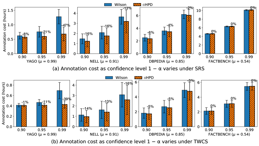
Figure 4. Annotation cost comparison between aHPD and Wilson at different confidence levels $1-\alpha$ under SRS (a) and TWCS (b) on YAGO, NELL, DBPEDIA, and FACTBENCH KGs. We also report the reduction ratio (in %) of aHPD over Wilson.

7. Related Work

The efficient evaluation of KGs accuracy has been largely overlooked. The first approach, KGEval (Ojha and Talukdar, 2017), is an iterative algorithm that alternates between control and inference stages. In the control stage, KGEval uses crowdsourcing to select facts for evaluation. In the inference stage, it applies type consistency and Horn-clause coupling constraints (Mitchell et al., 2018; Lao et al., 2011) to the evaluated facts to automatically estimate the correctness of additional facts. This process repeats until no more facts are evaluated. KGEval does not scale to real-life KGs (Gao et al., 2019) and is susceptible to error propagation due to its probabilistic inference mechanism, making it unsuitable for our work.

To overcome KGEval limitations, Gao et al. (2019) resorted to sampling strategies and estimators that gauge KG accuracy with statistical guarantees. To minimize annotation costs, (Gao et al., 2019) proposed the use of cluster sampling techniques (i.e., TWCS) over standard sampling (i.e., SRS). On the other hand, the authors relied on the Wald interval (Casella and Berger, 2002), known to have reliability issues when used on binomial proportions (Brown et al., 2001; Wallis, 2013). To address Wald issues for KG accuracy evaluation, Marchesin and Silvello (2024) proposed to use the Wilson interval (Wilson, 1927), being it better suited for binomial proportions.

Although reliable, the Wilson interval shares Wald’s frequentist interpretation, preventing a one-shot probabilistic understanding of its reliability. Additionally, the interval balances efficiency and reliability, sometimes requiring more annotations than Wald for greater reliability. In contrast, our solution offers a one-shot interpretation of interval confidence, making it better suited for the task while remaining the most efficient option. Moreover, the proposed approach, $a$HPD, eliminates the need for analysts to select a specific prior, addressing a key barrier to using Bayesian methods.

Qi et al. (2022) developed an efficient human-machine collaborative framework to minimize annotation costs through inference. This framework leverages statistical techniques similar to those in (Gao et al., 2019) and combines inference mechanisms akin to those in (Ojha and Talukdar, 2017). Their work focuses on the interplay between human annotations and inference mechanisms rather than on CIs and their impact on the minimization problem. Therefore, we do not include their method in our experimental analysis, but the $a$HPD method can be integrated into Qi et al. (2022)’s framework to enhance efficiency.

8. Conclusions

In this paper, we exposed the limitations of Confidence Intervals (CIs), used in current state-of-the-art solutions for evaluating KG accuracy. Rooted in frequentist statistics, these efficient intervals often lead to interpretation fallacies regarding confidence, precision, and likelihood, making them inconvenient for the task. We defined the interval estimation problem in Bayesian terms to address these limitations, introducing Bayesian Credible Intervals (CrIs). Using a prior distribution reflecting the initial belief about the KG accuracy and updating it with observed data through the likelihood, CrIs define the range of probable parameters in the posterior distribution. In other words, these intervals represent where the KG accuracy is likely to fall with $1-\alpha$ probability. Since they are built directly on the posterior distribution, CrIs avoid the interpretative pitfalls of CIs, offering reliable and efficient solutions in a one-shot setting.

We considered two families of CrIs: Equal-Tailed (ET) and Highest Posterior Density (HPD) intervals. Through theoretical and empirical analyses, we demonstrated that HPD CrIs represent the most efficient solution in real-life cases – where the KG accuracy is skewed – while remaining competitive with state-of-the-art in controlled scenarios – where the KG accuracy is (quasi-)symmetric.

We also addressed one of the major resistances to using Bayesian methods: the challenge of choosing the right prior. Prior selection is a critical aspect of Bayesian approaches, as selecting a poor prior can lead to deceptive interpretations or inefficient solutions. We proposed the adaptive HPD (aHPD) algorithm, where multiple objective priors are concurrently used to generate different $1-\alpha$ HPD intervals. These intervals compete to achieve convergence in the minimization problem, ensuring the most efficient outcome is always obtained from the set of competing solutions. In this way, aHPD removes the need to choose a specific prior in advance.

Through extensive experiments on both real and synthetic data, we showed that aHPD outperforms the state-of-the-art approaches across different scales, providing robust results regardless of the precision required for the evaluation process. Notably, aHPD reduced annotation costs by up to $47\%$ in high-precision scenarios. Based on this thorough evaluation, which involved both SRS and TWCS sampling strategies, we recommend that practitioners adopt aHPD with TWCS as the most efficient and reliable solution for auditing KG accuracy in a one-shot setting.

Future Work and Limitations

We plan to explore the use of the aHPD algorithm in dynamic environments, where KG contents evolve over time (Polleres et al., 2023). Consider a typical scenario for KGs, where batches of new content arrive at irregular intervals. Assume an initial evaluation has been conducted, resulting in a given KG accuracy estimate. When the volume of new content reaches a certain, predefined mass, we can perform a new evaluation. Leveraging the Bayesian framework we introduced to define the problem, we can consider the initial estimate as prior knowledge and use it as an informative prior for the new evaluation process. Equipped with reliable informative priors, aHPD can converge significantly faster than solutions based on uninformative priors (see Example 6).

Despite promising, this approach also hides potential limitations. Massive updates (e.g., half the size of the KG) with significantly different accuracy levels can render the informative prior less effective and, potentially, even deceptive. Exploring these challenges represents a critical direction for future research.

- (1)
- Auer et al. (2007) S. Auer, C. Bizer, G. Kobilarov, J. Lehmann, R. Cyganiak, and Z. G. Ives. 2007. DBpedia: A Nucleus for a Web of Open Data. In The Semantic Web, 6th International Semantic Web Conference, 2nd Asian Semantic Web Conference, ISWC 2007 + ASWC 2007, Busan, Korea, November 11-15, 2007 (LNCS, Vol. 4825). Springer, 722–735. doi:10.1007/978-3-540-76298-0_52
- Bayes (1763) T. Bayes. 1763. An Essay Towards Solving a Problem in the Doctrine of Chances. Phil. Trans. R. Soc. 53 (1763), 370–418. doi:10.1098/rstl.1763.0053
- Berger (1985) J. O. Berger. 1985. Statistical Decision Theory and Bayesian Analysis, 2nd Edition. Springer. doi:10.1007/978-1-4757-4286-2
- Bollacker et al. (2007) K. D. Bollacker, R. P. Cook, and P. Tufts. 2007. Freebase: A Shared Database of Structured General Human Knowledge. In Proc. of the Twenty-Second AAAI Conference on Artificial Intelligence, July 22-26, 2007, Vancouver, British Columbia, Canada. AAAI, 1962–1963. doi:10.5555/1619797.1619981
- Bollacker et al. (2008) K. D. Bollacker, C. Evans, P. K. Paritosh, T. Sturge, and J. Taylor. 2008. Freebase: A Collaboratively Created Graph Database for Structuring Human Knowledge. In Proc. of the ACM SIGMOD International Conference on Management of Data, SIGMOD 2008, Vancouver, BC, Canada, June 10-12, 2008. ACM, 1247–1250. doi:10.1145/1376616.1376746
- Bonifati et al. (2018) A. Bonifati, G. H. L. Fletcher, H. Voigt, and N. Yakovets. 2018. Querying Graphs. Morgan & Claypool Publishers. doi:10.2200/S00873ED1V01Y201808DTM051
- Box and Tiao (2011) G. E. P. Box and G. C. Tiao. 2011. Bayesian Inference in Statistical Analysis. John Wiley & Sons.
- Brown et al. (2001) L. D. Brown, T. T. Cai, and A. DasGupta. 2001. Interval Estimation for a Binomial Proportion. Statist. Sci. 16, 2 (2001), 101–117. http://www.jstor.org/stable/2676784
- Casella and Berger (2002) G. Casella and R. L. Berger. 2002. Statistical Inference. Thomson Learning. https://books.google.it/books?id=0x_vAAAAMAAJ
- Cochran (1977) W. G. Cochran. 1977. Sampling Techniques, 3rd Edition. John Wiley. doi:10.1017/S0013091500025724
- Deshpande et al. (2013) O. Deshpande, D. S. Lamba, M. Tourn, S. Das, S. Subramaniam, A. Rajaraman, V. Harinarayan, and A. Doan. 2013. Building, maintaining, and using knowledge bases: a report from the trenches. In Proc. of the ACM SIGMOD International Conference on Management of Data, SIGMOD 2013, New York, NY, USA, June 22-27, 2013. ACM, 1209–1220. doi:10.1145/2463676.2465297
- Edwards et al. (1963) W. Edwards, H. Lindman, and L. J. Savage. 1963. Bayesian Statistical Inference for Psychological Research. Psychol. Rev. 70, 3 (1963), 193–242. doi:10.1037/h0044139
- Esteves et al. (2018) D. Esteves, A. Rula, A. J. Reddy, and J. Lehmann. 2018. Toward Veracity Assessment in RDF Knowledge Bases: An Exploratory Analysis. ACM J. Data Inf. Qual. 9, 3 (2018), 16:1–16:26. doi:10.1145/3177873
- Gao et al. (2019) J. Gao, X. Li, Y. E. Xu, B. Sisman, X. L. Dong, and J. Yang. 2019. Efficient Knowledge Graph Accuracy Evaluation. Proc. VLDB Endow. 12, 11 (2019), 1679–1691. doi:10.14778/3342263.3342642
- Gelman (2008) A. Gelman. 2008. Rejoinder. Bayesian Anal. 3, 3 (2008), 467 – 477. doi:10.1214/08-BA318REJ
- Gerber et al. (2015) D. Gerber, D. Esteves, J. Lehmann, L. Bühmann, R. Usbeck, A. C. Ngonga Ngomo, and R. Speck. 2015. DeFacto - Temporal and multilingual Deep Fact Validation. J. Web Semant. 35 (2015), 85–101. doi:10.1016/j.websem.2015.08.001
- Hasibi et al. (2017) F. Hasibi, K. Balog, and S. E. Bratsberg. 2017. Dynamic Factual Summaries for Entity Cards. In Proc. of SIGIR. ACM, 773–782. doi:10.1145/3077136.3080810
- Hoekstra et al. (2014) R. Hoekstra, R. D. Morey, J. N. Rouder, and E. J. Wagenmakers. 2014. Robust Misinterpretation of Confidence Intervals. Psychon. Bull. Rev. 21 (2014), 1157–1164. doi:10.3758/s13423-013-0572-3
- Hoffart et al. (2013) J. Hoffart, F. M. Suchanek, K. Berberich, and G. Weikum. 2013. YAGO2: A spatially and temporally enhanced knowledge base from Wikipedia. Artif. Intell. 194 (2013), 28–61. doi:10.1016/j.artint.2012.06.001
- Ilyas et al. (2023) I. F. Ilyas, J. Lacerda, Y. Li, U. F. Minhas, A. Mousavi, J. Pound, T. Rekatsinas, and C. Sumanth. 2023. Growing and Serving Large Open-domain Knowledge Graphs. In Companion of the 2023 International Conference on Management of Data, SIGMOD/PODS 2023, Seattle, WA, USA, June 18-23, 2023. ACM, 253–259. doi:10.1145/3555041.3589672
- Ilyas et al. (2022) I. F. Ilyas, T. Rekatsinas, V. Konda, J. Pound, X. Qi, and M. A. Soliman. 2022. Saga: A Platform for Continuous Construction and Serving of Knowledge at Scale. In SIGMOD ’22: International Conference on Management of Data, Philadelphia, PA, USA, June 12 - 17, 2022. ACM, 2259–2272. doi:10.1145/3514221.3526049
- Jeffreys (1946) H. Jeffreys. 1946. An Invariant Form for the Prior Probability in Estimation Problems. Proc. R. Soc. A 186, 1007 (1946), 453–461. doi:10.1098/rspa.1946.0056
- Jin et al. (2017) S. Jin, M. Thulin, and R. Larsson. 2017. Approximate Bayesianity of Frequentist Confidence Intervals for a Binomial Proportion. Am. Stat. 71, 2 (2017), 106–111. doi:10.1080/00031305.2016.1208630
- Kerman (2011) J. Kerman. 2011. Neutral Noninformative and Informative Conjugate Beta and Gamma Prior Distributions. Electron. J. Stat. 5 (2011), 1450 – 1470. doi:10.1214/11-EJS648
- Kish (1965) L. Kish. 1965. Survey Sampling. Wiley. https://books.google.it/books?id=xiZmAAAAIAAJ
- Kish (1995) L. Kish. 1995. Methods for Design Effects. J. Off. Stat. 11, 1 (1995), 55. https://www.scb.se/contentassets/ca21efb41fee47d293bbee5bf7be7fb3/methods-for-design-effects.pdf
- Kraft (1988) D. Kraft. 1988. A Software Package for Sequential Quadratic Programming. Technical Report. DLR German Aerospace Center - Institute for Flight Mechanics, Koln, Germany. 1 – 33 pages.
- Lao et al. (2011) N. Lao, T. M. Mitchell, and W. W. Cohen. 2011. Random Walk Inference and Learning in A Large Scale Knowledge Base. In Proc. of the 2011 Conference on Empirical Methods in Natural Language Processing, EMNLP 2011, 27-31 July 2011, John McIntyre Conference Centre, Edinburgh, UK. ACL, 529–539. https://aclanthology.org/D11-1049/
- Lesaffre and Lawson (2012) E. Lesaffre and A. B. Lawson. 2012. Bayesian Biostatistics. John Wiley & Sons. doi:10.1002/9781119942412
- Makowski et al. (2019) D. Makowski, M. S. Ben-Shachar, and D. Lüdecke. 2019. bayestestR: Describing Effects and their Uncertainty, Existence and Significance within the Bayesian Framework. J. Open Source Softw. 4, 40 (2019), 1541. doi:10.21105/joss.01541
- Marchesin and Silvello (2024) S. Marchesin and G. Silvello. 2024. Efficient and Reliable Estimation of Knowledge Graph Accuracy. Proc. VLDB Endow. 17, 9 (2024), 2392–2404. doi:10.14778/3665844.3665865
- Marchesin et al. (2024a) S. Marchesin, G. Silvello, and O. Alonso. 2024a. Utility-Oriented Knowledge Graph Accuracy Estimation with Limited Annotations: A Case Study on DBpedia. Proc. of the 12th AAAI Conference on Human Computation and Crowdsourcing, HCOMP 2024, Pittsburgh, Pennsylvania, USA, October 16–19, 2024 12, 1 (2024), 105–114. doi:10.1609/hcomp.v12i1.31605
- Marchesin et al. (2024b) S. Marchesin, G. Silvello, and O. Alonso. 2024b. Veracity Estimation for Entity-Oriented Search with Knowledge Graphs. In Proc. of the 33rd ACM International Conference on Information and Knowledge Management, CIKM 2024, Boise, ID, USA, October 21-25, 2024. ACM, 1649–1659. doi:10.1145/3627673.3679561
- McElreath (2020) R. McElreath. 2020. Statistical Rethinking: A Bayesian Course with Examples in R and STAN. Chapman & Hall. doi:10.1201/9780429029608
- Mitchell et al. (2018) T. M. Mitchell, W. W. Cohen, E. R. Hruschka Jr., P. P. Talukdar, B. Yang, J. Betteridge, A. Carlson, B. D. Mishra, M. Gardner, B. Kisiel, J. Krishnamurthy, N. Lao, K. Mazaitis, T. Mohamed, N. Nakashole, E. A. Platanios, A. Ritter, M. Samadi, B. Settles, R. C. Wang, D. Wijaya, A. Gupta, X. Chen, A. Saparov, M. Greaves, and J. Welling. 2018. Never-ending learning. Commun. ACM 61, 5 (2018), 103–115. doi:10.1145/3191513
- Mohoney et al. (2023) J. Mohoney, A. Pacaci, S. R. Chowdhury, A. Mousavi, I. F. Ilyas, U. F.q Minhas, J. Pound, and T. Rekatsinas. 2023. High-Throughput Vector Similarity Search in Knowledge Graphs. Proc. ACM Manag. Data 1, 2 (2023), 197:1–197:25. doi:10.1145/3589777
- Morey et al. (2016) R. D. Morey, R. Hoekstra, J. N. Rouder, M. D. Lee, and E. J. Wagenmakers. 2016. The Fallacy of Placing Confidence in Confidence Intervals. Psychon. Bull. Rev. 23 (2016), 103–123. doi:10.3758/s13423-015-0947-8
- Navalpakkam et al. (2013) V. Navalpakkam, L. Jentzsch, R. Sayres, S. Ravi, A. Ahmed, and A. J. Smola. 2013. Measurement and modeling of eye-mouse behavior in the presence of nonlinear page layouts. In Proc. of WWW. International World Wide Web Conferences Steering Committee / ACM, 953–964. doi:10.1145/2488388.2488471
- Neyman (1941) J. Neyman. 1941. Fiducial Argument and the Theory of Confidence Intervals. Biometrika 32, 2 (1941), 128–150. http://www.jstor.org/stable/2332207
- Neyman and Jeffreys (1937) J. Neyman and H. Jeffreys. 1937. Outline of a Theory of Statistical Estimation Based on the Classical Theory of Probability. Philos. Trans. R. Soc. A 236, 767 (1937), 333–380. doi:10.1098/rsta.1937.0005
- Ojha and Talukdar (2017) P. Ojha and P. Talukdar. 2017. KGEval: Accuracy Estimation of Automatically Constructed Knowledge Graphs. In Proc. of the 2017 Conference on Empirical Methods in Natural Language Processing, EMNLP 2017, Copenhagen, Denmark, September 9-11, 2017. ACL, 1741–1750. doi:10.18653/v1/d17-1183
- Paulheim (2018) H. Paulheim. 2018. How much is a Triple? Estimating the Cost of Knowledge Graph Creation. In Proc. of the ISWC 2018 Posters & Demonstrations, Industry and Blue Sky Ideas Tracks co-located with 17th International Semantic Web Conference (ISWC 2018), Monterey, USA, October 8-12, 2018 (CEUR, Vol. 2180). CEUR-WS.org. https://ceur-ws.org/Vol-2180/ISWC_2018_Outrageous_Ideas_paper_10.pdf
- Polleres et al. (2023) A. Polleres, R. Pernisch, A. Bonifati, D. Dell’Aglio, D. Dobriy, S. Dumbrava, L. Etcheverry, N. Ferranti, K. Hose, E. Jiménez-Ruiz, M. Lissandrini, A. Scherp, R. Tommasini, and J Wachs. 2023. How Does Knowledge Evolve in Open Knowledge Graphs? TGDK 1, 1 (2023), 11:1–11:59. doi:10.4230/TGDK.1.1.11
- Press (2002) S. J. Press. 2002. Subjective and Objective Bayesian Statistics: Principles, Models, and Applications. John Wiley & Sons. doi:10.1002/9780470317105
- Pujara et al. (2017) J. Pujara, E. Augustine, and L. Getoor. 2017. Sparsity and Noise: Where Knowledge Graph Embeddings Fall Short. In Proc. of the 2017 Conference on Empirical Methods in Natural Language Processing, EMNLP 2017, Copenhagen, Denmark, September 9-11, 2017. ACL, 1751–1756. doi:10.18653/v1/d17-1184
- Qi et al. (2022) Y. Qi, W. Zheng, L. Hong, and L. Zou. 2022. Evaluating Knowledge Graph Accuracy Powered by Optimized Human-Machine Collaboration. In KDD ’22: The 28th ACM SIGKDD Conference on Knowledge Discovery and Data Mining, Washington, DC, USA, August 14 - 18, 2022. ACM, 1368–1378. doi:10.1145/3534678.3539233
- Raiffa and Schlaifer (1961) H. Raiffa and R. Schlaifer. 1961. Applied Statistical Decision Theory. Division of Research, Graduate School of Business Adminitration, Harvard University. https://books.google.it/books?id=wPBLAAAAMAAJ
- Reinanda et al. (2020) R. Reinanda, E. Meij, and M. de Rijke. 2020. Knowledge Graphs: An Information Retrieval Perspective. Found. Trends Inf. Retr. 14, 4 (2020), 289–444. doi:10.1561/1500000063
- Samadi et al. (2015) M. Samadi, P. P. Talukdar, M. M. Veloso, and T. M. Mitchell. 2015. AskWorld: Budget-Sensitive Query Evaluation for Knowledge-on-Demand. In Proc. of the Twenty-Fourth International Joint Conference on Artificial Intelligence, IJCAI 2015, Buenos Aires, Argentina, July 25-31, 2015. AAAI Press, 837–843. http://ijcai.org/Abstract/15/123
- Vrandecic and Krötzsch (2014) D. Vrandecic and M. Krötzsch. 2014. Wikidata: a free collaborative knowledgebase. Commun. ACM 57, 10 (2014), 78–85. doi:10.1145/2629489
- Wallis (2013) S. Wallis. 2013. Binomial Confidence Intervals and Contingency Tests: Mathematical Fundamentals and the Evaluation of Alternative Methods. J. Quant. Linguistics 20, 3 (2013), 178–208. doi:10.1080/09296174.2013.799918
- Wasserman (2008) L. Wasserman. 2008. Comment on Article by Gelman. Bayesian Anal. 3, 3 (2008), 463 – 465. doi:10.1214/08-BA318D
- Wilson (1927) E. B. Wilson. 1927. Probable Inference, the Law of Succession, and Statistical Inference. J. Amer. Statist. Assoc. 22, 158 (1927), 209–212. doi:10.1080/01621459.1927.10502953
- Xue and Zou (2023) B. Xue and L. Zou. 2023. Knowledge Graph Quality Management: A Comprehensive Survey. IEEE Trans. Knowl. Data Eng. 35, 5 (2023), 4969–4988. doi:10.1109/TKDE.2022.3150080