Functional interpolation expansion for nonequilibrium correlated impurities

Abstract

We present a functional interpolation approach within the auxiliary master equation framework to efficiently and accurately solve correlated impurity problems in nonequilibrium dynamical mean-field theory (DMFT). By leveraging a near-exact auxiliary bath representation, the method estimates corrections via interpolation over a few bath realisations, significantly reducing computational cost and increasing accuracy. We illustrate the approach on the Anderson impurity model and on the Hubbard model within DMFT, capturing equilibrium and long-lived photodoped states.

Introduction

Advances in controlling quantum materials, ranging from ultrafast laser spectroscopy, [1, 2, 3, 4] solid state nanocience, [5, 6] and ultracold quantum gases [7, 8, 9, 10] have sparked growing interest in nonequilibrium strongly correlated systems. These developments drive theoretical challenges, including understanding nonequilibrium quantum phase transitions, [11] thermalization, and decoherence [12, 13, 14, 15]. In this context, the theoretical description of strongly correlated quantum systems out of equilibrium remains an exciting challenge in modern theoretical physics.

The extension of dynamical mean-field theory (DMFT) [16, 17] to nonequilibrium [18, 19, 20, 21, 22, 23, 24] provides a key framework for addressing these systems. DMFT in the time domain has been applied to simulate a variety of phenomena and systems ranging from highly excited states in photoexcited materials to ultracold atoms or Mott insulators under strong DC fields (see, e.g. Ref.[24]). The main bottleneck of DMFT, the solution of a many-body quantum impurity, is a long-standing problem for nonequilibrium systems. Exact quantum Monte Carlo (QMC) [25, 26] or matrix-product states [27, 28] calculations are limited to short time so that mostly low-order hybridization expansions, such as the non-crossing approximation are adopted in practice. When restricting to the steady state, advances have been achieved, among others, via the QMC inchworm [29], scattering-states approaches [30, 31], or the auxiliary master equation (AMEA) [32, 33] algorithms.

Steady-state algorithms provide a complement to real-time simulations as they can be used to address the slowly time-evolving regime occurring, for instance in photoexcited Mott insulators after an initial prethermalisation phase [34, 35, 36, 37, 38]. While this regime cannot be reliably addressed by numerically exact real-time approaches, one can adopt a time-local ansatzt for the fermionic distribution function of a reference steady-state system [39] which then evolves in time following a generalized quantum Boltzmann scheme [40].

It is therefore crucial to develop nonperturbative, accurate methods that remain computationally efficient enough to be used as quantum impurity solvers in DMFT self-consistent calculations.

The approach presented in this Letter exploits the freedom to replace the “physical” fermionic bath of the impurity problem that needs to be solved, e.g. at each DMFT step, with a so-called “auxiliary” one consisting of a small number $N_{\text{b}}$ (typically $6$ to $8$) of bath sites connected to a Markovian environment which then can be solved exactly by numerical methods. Since the “residual” distance (termed $\underline{\varepsilon}$ below) between the hybridization functions of the two baths is exponentially small in $N_{\text{b}}$ [41] a substantial improvement by including perturbative corrections in $\underline{\varepsilon}$ can be obtained, see Ref. [42] for a similar idea. However, for values of $N_{\text{b}}\gtrsim 6$ for which $\underline{\varepsilon}$ is small enough, this expansion becomes prohibitive and computationally quite expensive. The main idea presented here consists in adopting a Functional interpolation (FI) approach which amounts in estimating the $\underline{\varepsilon}$ linear corrections by a solution of the impurity problem for a few (typically two to four) different suitably chosen sets of bath parameters.

After testing the approach for the Anderson impurity model in and out of equilibium, we address, within DMFT, the Hubbard model on both sides of the equilibrium Mott phase, as well as the long-lived nonequilibrium photodoped state.

Model and Method

A fermionic single-impurity problem is fully characterized by its impurity hamiltonian $H_{\text{imp}}$ typically describing electrons on a single orbital with an onsite interaction $U$. The coupling of this orbital to a noninteracting fermionic bath is completely characterized by its hybridization function $\underline{\Delta}_{\text{phys}}(\omega)$, which in a nonequilibrium steady state consists of a $2\times 2$ matrix in Keldysh space [43, 44, 45, 46, 47] .

Within AMEA [32, 33] this “physical” hybridization function $\underline{\Delta}_{\text{phys}}(\omega)$ is approximated by the hybridization function

$$\underline{\Delta}_{\text{aux}}(\omega)=\underline{\Delta}_{\text{phys}}(\omega)+\underline{\varepsilon}(\omega)$$ (1)

of an “auxiliary”

bath consisting of a finite number $N_{\text{b}}$ of bath sites connected to a Markovian environment, whose dynamics is described by the Lindblad equation, see  [33, 32]. For a sufficiently small $N_{\text{b}}$, the impurity problem connected to the auxiliary bath can be solved exactly, for example, by Lanczos/Arnoldi-like methods [33, 49], by matrix-product states (MPS) [50] or by stochastic wave function approaches [51]. In principle, in the $\underline{\varepsilon}\to 0$ limit the computed interacting impurity Green’s function of this auxiliary system approaches the physical one for any value of $U$. A clever choice of the (Lindblad) parameters [41] of the auxiliary bath obtained, e.g., by fitting $\underline{\Delta}_{\text{aux}}$ to $\underline{\Delta}_{\text{phys}}$ makes $|\underline{\varepsilon}|$ to vanish exponentially in terms of $N_{\text{b}}$ [41]. Here $|\underline{\varepsilon}|$ is some measure of the norm of the deviation $\underline{\varepsilon}$ integrated over frequencies possibly with some weight factor $W(\omega)$ to emphasize some physical relevant frequency regions.

Unfortunately, since one must consider the full space of many-body density matrices, the maximum $N_{\text{b}}$ that can be achieved by Lanczos-like methods  is restricted to $N_{\text{b}}\approx 8-10$. While MPS approaches can address larger systems, the geometry restriction makes the fit less efficient [41]. We, therefore, propose to improve the accuracy by including corrections of $O(\underline{\varepsilon}^{1})$. In principle, this is the spirit of hybridization expansion methods for example the non-crossing approximation (NCA) [53, 54, 55], which corresponds, formally, to taking $\underline{\varepsilon}=\underline{\Delta}_{\text{phys}}$ in (1). However, since $\underline{\varepsilon}$ is not small in this case, only higher orders, provide reliable results. For these one has to resort to, e.g., Quantum Monte Carlo [26, 56, 29] or, as shown recently, to tensor trains [57, 58].

In Ref. [59] it was suggested to carry out a dual-fermion expansion around a “better” solution with a $\underline{\Delta}_{\text{aux}}$ closer to the physical one obtained with an auxiliary bath with $N_{\text{b}}=2$. While the results of the expansion display a significant improvement with respect to the one of the plain auxiliary system , an extension to larger $N_{\text{b}}$ is quite prohibitive. This is due to the fact that one needs to evaluate a three-point vertex, which is numerically complicated in Lanczos/Arnoldi. On the other hand, only values of $N_{\text{b}}\gtrsim 6$ guarantee that $\underline{\varepsilon}$ is sufficiently small so that a first order expansion is justified. Here, we follow a different path and estimate the $O(\underline{\varepsilon}^{1})$ term numerically by solving the nonequilibrium impurity problem for a batch of $\underline{\varepsilon}$. We exploit the fact that, for fixed $H_{\text{imp}}$ the steady-state self energy $\underline{\Sigma}$ is a functional of $\underline{\Delta}$ only. Therefore, to first order in $\underline{\varepsilon}$ we can write

$$\underline{\Sigma}[\underline{\Delta}_{\text{phys}}+\underline{\varepsilon}]=\underline{\Sigma}[\underline{\Delta}_{\text{phys}}]+\frac{\delta\underline{\Sigma}[\underline{\Delta}_{\text{phys}}]}{\delta\underline{\Delta}_{\text{phys}}}\odot{\underline{\varepsilon}}+O(\underline{\varepsilon})^{2}.$$ (2)

Strictly speaking, the independent functions in the argument of $\underline{\Sigma}$ are just $\operatorname*{Im}\Delta^{\text{R}}(\omega)$ and $\operatorname*{Im}\Delta^{\text{K}}(\omega)$, as $\operatorname*{Re}\Delta^{\text{R}}$ is fixed by Kramers-Krönig and $\operatorname*{Re}\Delta^{\text{K}}=0$. Therefore, we will understand the functional dependence, and corresponding derivative, with respect to these functions only. Similarly, $\odot$ indicates a convolution, i.e. a sum over these two components and an integral over $\omega$. An equation like (2) is obviously valid for the Green’s function as well. Here, we will limit the discussion to the self-energy.

To start with, let us first hypothetically assume that, in addition to (1), one could compute the self energy for a different “desired” hybridization

$$\underline{\Delta}_{\text{des}}=\underline{\Delta}_{\text{phys}}+k\ \underline{\varepsilon}$$ (3)

with some real number $k$ away from 1. Then, by applying (2) for $\underline{\varepsilon}$ replaced with $k\cdot\underline{\varepsilon}$ one can cancel the first order errors exactly yielding

$$\underline{\Sigma}[\underline{\Delta}_{\text{phys}}]=\frac{1}{1-k}\left(\underline{\Sigma}[\underline{\Delta}_{\text{phys}}+k\ \underline{\varepsilon}]-k\ \underline{\Sigma}[\underline{\Delta}_{\text{phys}}+\underline{\varepsilon}]\right)+O(\underline{\varepsilon}^{2}),$$ (4)

For example, for $k=-1$ this is the average between the two self-energies at $\underline{\Delta}_{\text{phys}}\pm\underline{\varepsilon}$.

The problem is that, in general, $\underline{\Delta}_{\text{des}}$ will not be representable within an auxiliary bath with finite $N_{\text{b}}$ in the sense that there is no set of Lindblad parameters producing it.

An alternative “bottom-up” approach consists in generalizing (4) to a set of $n_{\max}$ different suitably chosen auxiliary baths with the same $N_{\text{b}}$ but with different parameters. The deviations $\underline{\varepsilon}_{n}$ of their hybridization functions from the physical one

$$\underline{\varepsilon}_{n}=\underline{\Delta}_{\text{phys}}-{\underline{\Delta}_{\text{aux}}}_{n}\quad\quad n=1,\cdots,n_{\max}\;.$$ (5)

must remain small, i.e. of the same order of magnitude.

One can then determine coefficients $\alpha_{n}$ such that the quantity

$$\underline{\mu}\equiv\sum_{n=1}^{n_{\max}}\alpha_{n}\ \underline{\varepsilon}_{n}\quad\text{with}\quad\sum_{n=1}^{n_{\max}}\alpha_{n}=1$$ (6)

is much smaller than the $\underline{\varepsilon}_{n}$. Here, $\underline{\mu}(\omega)$ controls the “residual” first-oder error in an improved approximation for the self-energy of the physical system

$$\Sigma[\underline{\Delta}_{\text{phys}}]=\sum_{n=1}^{n_{\max}}\alpha_{n}\ \underline{\Sigma}[\underline{\Delta}_{\text{phys}}+\underline{\varepsilon}_{n}]+O(\underline{\mu})+O(\underline{\varepsilon}^{2})\;.$$ (7)

The optimal coefficients $\alpha_{n}$ should be, thus, chosen such that

$$|\underline{\mu}|^{2}=\sum_{m,n=1}^{n_{\max}}\alpha_{n}\alpha_{m}A_{mn}\quad\quad A_{mn}\equiv\underline{\varepsilon}_{n}\odot\underline{\varepsilon}_{m}$$ (8)

is minimal. The constraint in (6) can be addressed via a Lagrange multiplier $\lambda$ leading to the optimal values

$$\bm{\alpha}=\lambda\bm{A}^{-1}\cdot\bm{u}\quad\quad\lambda=\left(\bm{u}^{T}\cdot\bm{A}^{-1}\bm{u}\right)^{-1}$$ (9)

with $\bm{u}^{T}=(1,1,1,\dots)$.

We have tried two different procedures to select the set of ${\underline{\Delta}_{\text{aux}}}_{n}$in (5), or, equivalently $\underline{\varepsilon}_{n}$. The first one is deterministic and consists in the following steps: We start by finding the (Lindblad) parameters of the auxiliary bath that give the best fit to ${\underline{\Delta}_{\text{phys}}}$. The correspondig hybridization function is assigned to ${\underline{\Delta}_{\text{aux}}}_{m}$ with $m=1$.
(i) For a given ${\underline{\Delta}_{\text{aux}}}_{m}$ we extract the corresponding $\underline{\varepsilon}_{m}$ from (5) and construct the corresponding $\underline{\mu}$ from (6) and (9) with $n_{\max}=m$.
(ii) We use this $\underline{\mu}$, which we name $\underline{\mu}_{m}$, to determine a new ${\underline{\Delta}_{\text{aux}}}_{m+1}$ by fitting the Lindblad parameters to a “desired” ${\underline{\Delta}_{\text{des}}}_{m+1}=\underline{\Delta}_{\text{phys}}+k\ \underline{\mu}_{m}$ (cf. (3)). Here, $k$ is some number  sufficiently away from $1$. This choice is motivated by the fact that if one could fit $\underline{\Delta}_{\text{des}}$ exactly, the first order error would be canceled, similarly to (4). With the new ${\underline{\Delta}_{\text{aux}}}_{m+1}$ we go back to step (i).
Steps (i) to (ii) should be repeated up to a maximum value $N_{\text{T}}$ for $m$ or until the condition number  of the matrix $A$ exceeds a given value. Finally, the improved self-energy is obtained via (7).

A modification of this procedure consists in starting with two (or more) different initial ${\underline{\Delta}_{\text{aux}}}_{m=1}$ obtained by different fits, i.e. using different weight functions $W(\omega)$. Then the corresponding $\underline{\varepsilon}_{m}$ are combined together in (7). Alternatively, starting with the same ${\underline{\Delta}_{\text{aux}}}_{m=1}$ as for the previous algorithm, one can adopt a random procedure for determining the $\underline{\varepsilon}_{m}$ for $m>1$. This is achieved by replacing the $N_{\text{T}}$ “desired” hybridization functions of step (ii) in the previous procedure by random functions sufficiently close to $\underline{\Delta}_{\text{phys}}(\omega)$.   Since this is a random procedure, it may be convenient to repeat it a certain number of times $N_{\text{av}}$ and average the corresponding results for the self energy.

Results

Since we have a certain freedom in choosing the details of the procedure, such as the value of $k$ and $N_{\text{T}}$ or whether to use the deterministic or the random version, it is convenient to first test different options in order to find out the most efficient and accurate one. We do this by applying the approach for numerically “cheap” auxiliary baths with $N_{\text{b}}=4$ and compare the self-energy obtained in this way with a reference evaluated with the plain  $N_{\text{b}}=8$ one which is expected to be more accurate than the $N_{\text{b}}=4$ case. The benchmark reported in the supplemental material [65] suggests that the best accuracy is obtained with the deterministic algorithm with $k=2$ and $N_{\text{T}}=2$. This is interesting, as it shows that we can substantially increase the accuracy of the impurity solver by just carrying out two Lindblad many-body calculations. In particular, as we will see below, a many-body calculation with $N_{\text{b}}=6$ using the present FI approach yields an accuracy comparable or better than a plain $N_{\text{b}}=8$ one, which is approximately $6$ times as costly. In addition, the two many-body calculations required by the FI approach can be done in parallel. This is particularly convenient when using it as an impurity solver for Dynamical Mean-Field Theory (DMFT)

We start by computing the spectral function for an Anderson impurity in and out of equilibrium. Unless otherwise specified, we consider a bath with a flat density of states (DOS) of width $10\Gamma$  with the following parameters $U/\Gamma=6$, $-\operatorname*{Im}\Delta^{\text{R}}(\omega=0)/\Gamma=1$, $\varepsilon_{\text{imp}}=-U/2$. In Fig. 1 we display the spectral function of the impurity coupled to (a) a bath in equilibrium at temperature $T/\Gamma=0.02$ and (b) to two baths with a bias voltage $V/\Gamma=1.5$. As one can see, the results with $N_{\text{b}}=6$ augmented with the FI approach is in some cases even more accurate than the plain $N_{\text{b}}=8$, as the comparison with Numerical Renormalisation Group (NRG) shows. FI combined with $N_{\text{b}}=8$ provides an even better accuracy. Of course, in equilibrium the method cannot compete with NRG, but it has the advantage that it can be straightforwadly extended to nonequilibrium steady states.

Figure 1: Spectral function of the equilibrium (a) Anderson impurity model for $U/\Gamma=6$, $-\operatorname*{Im}\Delta^{\text{R}}(\omega=0)/\Gamma=1$, $\varepsilon_{\text{imp}}=-U/2$, and $T/\Gamma=0.02$ obtained by plain AMEA with $N_{\text{b}}=6$ and $N_{\text{b}}=8$ and improved results obtained by the FI approach with $k=2$ and $N_{\text{T}}=2$ for the two cases. (b) shows the same results for the case of a finite bias voltage $V/\Gamma=1.5$. The equilibrium ($V/\Gamma=0$) results are compared with NRG.

As mentioned above, the greatest advantage of the approach consists in its application as an efficient impurity solver for steady-state nonequilibrium DMFT. The method is also quite convenient as a real-frequency impurity solver in the equilibrium case. To illustrate this, we apply it to the infinite-dimensional Hubbard model with the Bethe lattice DOS. We start by addressing the most challenging regime in the equilibrium case, i.e. the vicinity of the metal-insulator transition. We take a point in the metallic phase at $T/\Gamma=0.05$ and $U/\Gamma=4.4$ and one nearby for $U/\Gamma=5.0$ and the same temperature in the insulating phase. The corresponding spectral functions are plotted in figure 2. In both cases the results obtained for $N_{\text{b}}=6$ FI lead to a significant improvement, i.e., they give a solution closer to $N_{\text{b}}=8$ than the plain $N_{\text{b}}=6$. At the same time, the $N_{\text{b}}=8$ FI result shows a more pronounced quasiparticle peak in the metallic and a clearer gap in the insulating phase.

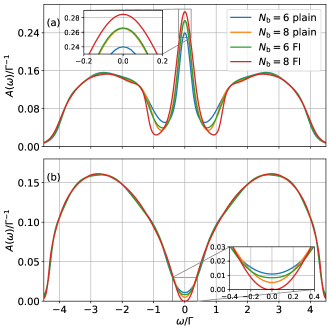
Figure 2: Spectral function for the infinite-dimensional Bethe lattice at $T/\Gamma=0.05$, $\varepsilon_{\text{imp}}=-U/2$, $t/\Gamma=1$, and (a) $U/\Gamma=4.4$, i.e. in the metallic phase, or (b) for a point in the insulating phase at $U/\Gamma=5$.

As a benchmark for a steady-state nonequilibrium situation we address cold photodoped states in a Mott insulator [34, 35, 36, 37]. In Ref. [39] it has been shown that these long-lived states can be reliably described by a time-local quasi-steady-state ansatz for which numerically exact inchworm Monte Carlo data have been produced. In Fig. 3 we compare the self-energy obtained by AMEA with $N_{\text{b}}=6$ and $8$ along with the corresponding FI corrections with the inchworm data from Ref. [39]. As one can see, the FI $N_{\text{b}}=8$ calculation produces a peak which is very close to the inchworm one. On the other hand, the vanishing of the self-energy at the quasiparticle chemical potential around $\omega/\Gamma\approx\pm 1.82$ is harder to reproduce. This is probably due to the fact that since the self-energy vanishes quadratically there, some kind of quadratic (instead of linear, as in (2)) extrapolation should be carried out.

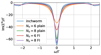
Figure 3: Imaginary part of the self-energy of a cold photodoped quasi steady state obtained by the FI approach and plain AMEA compared with inchworm QMC data (extracted from Ref. [39]). Parameters are as Fig. 2b of Ref. [39].

Conclusion

We have introduced an approach for solving many-body impurity problems, particularly suited for strongly correlated systems out of equilibrium within dynamical mean-field theory. The method involves exactly solving the impurity embedded in a small auxiliary bath coupled to a Markovian environment, then applying a linear correction for the difference between the auxiliary and physical baths. This correction is well-justified when the difference between the two baths is small, as achieved with $N_{\text{b}}=6-8$. Our approach significantly improves results over a plain AMEA DMFT impurity solver in and out of equilibrium.

One key advantage of the present FI approach is that good accuracy is achieved with as few as $N_{\text{b}}=6$ bath sites, significantly speeding up impurity computations, which is crucial for DMFT self-consistency. Moreover, the ability to use fewer bath sites makes the method extendable to multi-orbital systems, which is essential for first-principles studies of correlated materials.

While the “FI” expression (7) is straightforward, in practice the achieved accuracy sometimes depends on the choice of the batch of $N_{\text{T}}$ auxiliary hybridization functions. Our extensive analysis for $N_{\text{b}}=4$ suggests that a substantial improvement is obtained already with $N_{\text{T}}=2$. The question is whether this conclusion is valid (a) also for larger $N_{\text{b}}$ and (b) for more structured hybridization functions. Increasing $N_{\text{T}}$ improves the accuracy of the self-energy in (7) because it reduces $|\underline{\mu}|$. However, when $|\underline{\mu}|$ becomes smaller or of the order of $|\underline{\varepsilon}|^{2}$, the error gets dominated by the latter and there is no point of further reducing $|\underline{\mu}|$. This may suggest that larger $N_{\text{T}}$ could be necessary when using $N_{\text{b}}\gtrsim 6$ for which $|\underline{\varepsilon}|$ is smaller. In the case of a structured (physical) hybrization function, the FI approach could provide a receipt to cleverly combine the result of auxiliary hybridization functions adapted to one or to the other region. In this case, increasing $N_{\text{T}}$ should also improve the results. These issues should be addressed in future studies.

Appendix A Supplemental material

Since we have a certain freedom in choosing the details of the procedure, such as in the choice of $k$ or whether to use the deterministic or the random procedure described in the main text, it is convenient to first test different options in order to find out the most convenient one. We do this by applying the approach for the numerically “cheap” case of an auxiliary bath with $N_{\text{b}}=4$ and compare the self-energy obtained in this way with a reference evaluated with “plain” $N_{\text{b}}=8$ which is expected to be more accurate even without this FI procedure.

Unless otherwise specified, we consider a bath with a flat DOS of width $10\Gamma$ with the following parameters $U/\Gamma=6$, $-\operatorname*{Im}\Delta^{\text{R}}(\omega=0)/\Gamma=1$, $\varepsilon_{\text{imp}}=-U/2$, $T/\Gamma=0.05$. Moreover we denote $N_{\text{T}}$ as the maximum number of auxiliary systems included in the sum (7), corresponding to a set of deviations

$$\{\underline{\varepsilon}_{1},\underline{\varepsilon}_{2},\cdots,\underline{\varepsilon}_{N_{\text{T}}}\}.$$

Similarly, we denote by $\underline{\mu}_{n_{\max}}$ the corresponding optimized deviations (6) for $n_{\max}=1,\cdots,N_{\text{T}}$.

As mentioned in the results section we compare self energies with $N_{\text{b}}=4$ and different versions of the FI approach with the ones obtained with “plain” eight bath sites ($N_{\text{b}}=8$) (i.e. no FI procedure). Since the “plain” $N_{\text{b}}=8$ results are expected to be very accurate, this provides an error estimate for the $N_{\text{b}}=4$ FI calculations as

$$\begin{split}\chi_{\Sigma}=&\frac{1}{2\omega_{\text{max}}}\int_{\omega=-\omega_{\text{max}}}^{\omega=\omega_{\text{max}}}\Bigl{(}|\operatorname*{Im}(\Sigma^{\text{R}}_{N_{\text{b}}=8})-\operatorname*{Im}(\Sigma^{\text{R}}_{N_{\text{b}}=4,\text{FI}})|^{2}\\ &+|\operatorname*{Im}(\Sigma^{\text{K}}_{N_{\text{b}}=8})-\operatorname*{Im}(\Sigma^{\text{K}}_{N_{\text{b}}=4,\text{FI}})|^{2}\Bigr{)}d\omega.\end{split}$$ (10)

For the deterministic algorithm described in the text we try the factors $k=-1$ and $k=2$. Table 4(a) shows that using $k=-1$ the FI approach gives no improvement, whereas from table 4(b) it becomes evident, that $k=+2$ produces a strong reduction of $\chi_{\Sigma}$ over the full voltage range. On the other hand, we notice that increasing $N_{\text{T}}$ beyond $2$ hardly produce any improvement. This is an important result which suggests that in fact it is sufficient to solve for two impurity solvers in order to substantially improve the accuracy of the calculation. Of course this is valid for the present model with a flat band. The story may be different for a more subtle density of states. This will be the goal of future investigations.

It is, nevertheless, important to understand the reasons behind this behavior.

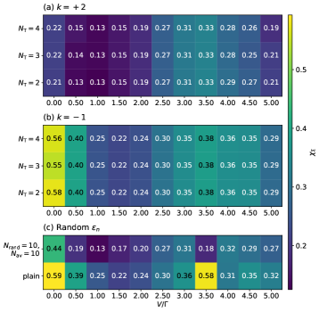
Figure 4: Error $\chi_{\Sigma}$ (Eq. 10) of results obtained using four bath sites ($N_{\text{b}}=4$) in combination with the FI based approach at $T/\Gamma=0.05$ and voltage drop ranging from $V/\Gamma=0$ to $5$ in steps of $0.5$. (a) and (b) use the deterministic algorithm (see text) and (c) uses the “random” one. In (a) we use $k=2$, while in (b) we use $k=-1$.

First, we want to understand, why $k=2$ is more accurate than $k=-1$. $k=2$ means that the $m=2$ hybridization ${\underline{\Delta}_{\text{des}}}_{2}$ is farther away from the pyhsical one than the $m=1$ one. On the other hand, $k=-1$ corresponds to a ${\underline{\Delta}_{\text{des}}}_{2}$ on the “other side” of the physical one. So, why is it more convenient to go “further away” from the correct hybridization rather than to go “to the other side”? In order to address this, we look at the “desired” hybridization functions (${\underline{\Delta}_{\text{des}}}_{2}=\underline{\Delta}_{\text{phys}}+k\underline{\mu}_{1}$) and the corresponding fitted ones (${\underline{\Delta}_{\text{aux}}}_{2}$) for $N_{\text{T}}=2$. The imaginary part of their retarded component are shown in figure 5 (a) for $k=+2$ and in 5 (b) for $k=-1$  and compared with the physical hybridization ${\underline{\Delta}_{\text{phys}}}(={\underline{\Delta}_{\text{des}}}_{1})$ and the first auxiliary one ${\underline{\Delta}_{\text{aux}}}_{1}$. The figures clearly show that the fit to ${\underline{\Delta}_{\text{des}}}_{2}$ is far more accurate for $k=+2$ than for $k=-1$. The reason for this better fit is due to the fact that the desired hybridization function for $k=+2$ simply amplifies the features of the first fit (${\underline{\Delta}_{\text{aux}}}_{1}$).

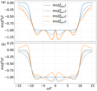
Figure 5: $\operatorname*{Im}({\Delta^{\text{R}}_{\text{aux}}}_{2})$ (orange, dashed) fitted to the corresponding “desired” $\operatorname*{Im}({\Delta^{\text{R}}_{\text{des}}}_{2})$ (orange, solid) with $k=2$ (a) and $k=-1$ (b). For $k=2$ the fit is extremely accurate, in contrast to $k=-1$. Both curves also show $\operatorname*{Im}({\Delta^{\text{R}}_{\text{aux}}}_{1})$ and $\operatorname*{Im}({{\Delta^{\text{R}}_{\text{phys}}}})$ for comparison

We now address the question why including more than two $\underline{\Delta}_{\text{aux}}$ in (7) doesn’t improve the accuracy of the self-energy. Similarly to the previous analysis, in Fig. 6 we plot the “desired” ${\underline{\Delta}_{\text{des}}}_{m}=\underline{\Delta}_{\text{phys}}+k\underline{\mu}_{m-1}$ (solid line) along with its corresponding fit ${\underline{\Delta}_{\text{aux}}}_{m}$ (dashed line with same color). We restrict to the imaginary part of the retarded component.

We fix $k=2$, as suggested by the previous analysis and we show the results for $m=2$ and $m=3$ with $N_{\text{T}}=3$. As one can see, while the fit to the ${\Delta^{\text{R}}_{\text{des}}}_{2}$ curve is excellent, the one to the ${\Delta^{\text{R}}_{\text{des}}}_{3}$ curve is quite poor. As a consequence, inclusion of ${\underline{\Delta}_{\text{aux}}}_{3}$ and corresponding $\underline{\varepsilon}_{3}$ (cf. (5)) does not make $\underline{\mu}$ (6) smaller and, consequently, does not produce a more accurate self-energy ((7)).

Figure 6: $\operatorname*{Im}({\Delta^{\text{R}}_{\text{des}}}_{m})$ (solid) as well as its fit $\operatorname*{Im}({\Delta^{\text{R}}_{\text{aux}}}_{m})$ (dashed) for $m=2$ (blue) and $3$ (orange). While the fit for $m=2$ shows almost perfect coincidence, the one for $m=3$ is quite poor, thus providing no improvement in the FI procedure.

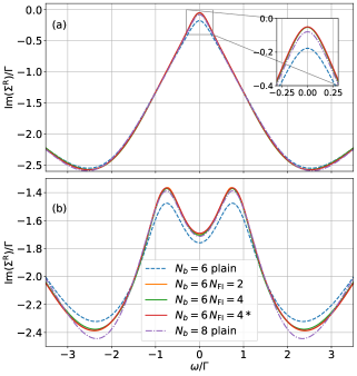
Figure 7: Comparison of plain calculations with those obtained via the FI approach for $V/\Gamma=0$ (a) and $V/\Gamma=1.5$ (b). $\operatorname*{Im}(\Sigma^{\text{R}})$ for $N_{\text{b}}=6$ does not change significantly when increasing the number of included hybridization functions. The $N_{\text{T}}=4*$ results have been obtained by combining two $N_{\text{T}}=2$ sets of hybridization functions with weights in the fit (see text).

This may change when using more bath sites $N_{\text{b}}>4$, since one can better reproduce subtle features. To investigate this, we show in figure 7 results for $N_{\text{b}}=6$ at $T/\Gamma=0.02$ and $V/\Gamma=0$ (a) and $V/\Gamma=1.5$ (b) respectively. Here we compare the self-energy obtained with $N_{\text{T}}=2$ with the one obtained with two additional steps ($N_{\text{T}}=4$) of the deterministic algorithm. This figure also includes a plot (termed $N_{\text{T}}=4*$) where we combined two $N_{\text{T}}=2$ sets of hybridization functions, where the second set used weights  in the fit of the hybridization functions. Comparison with the benchmark ($N_{\text{b}}=8$) shows that even in this case there is no improvement upon increasing $N_{\text{T}}$. Therefore, we will use $N_{\text{T}}=2$ for the deterministic algorithm. The results also show a significant improvement with respect to the plain AMEA result, thus emphasizing the importance of using the FI approach even by evaluating just one more hybridization function.

To test the “random” algorithm we choose

$$\operatorname*{Im}{\Delta^{\text{R/K}}_{\text{des}}}_{m}=\operatorname*{Im}\Delta^{\text{R/K}}_{\text{phys}}+f_{\text{rand}}^{\text{R/K}}(\omega)\ \ \ \forall\ m>1$$ (11)

with $f_{\text{rand}}^{\text{R/K}}(\omega)$ having five equidistant points between $-\omega_{\text{max}}$ and $\omega_{\text{max}}$, where at each point a random value between $-0.3$ and $0.3$ is taken and the space in between is smoothly interpolated. Figure 4 (c) shows the error $\chi_{\Sigma}$ in the self-energy for this algorithm. We used $N_{\text{T}}=10$ and $N_{\text{av}}=10$. The results show a clear improvement with respect to the plain case, but mostly less than the one obtained by the deterministic algorithm with $k=+2$, (cf. Fig. 4(a)) which is also computationally much less costly. For this reason, in this paper we adopt the deterministic algorithm with $k=2$.

References

- Iwai et al. [2003] S. Iwai, M. Ono, A. Maeda, H. Matsuzaki, H. Kishida, H. Okamoto, and Y. Tokura, Ultrafast optical switching to a metallic state by photoinduced mott transition in a halogen-bridged nickel-chain compound, Phys. Rev. Lett. 91, 057401 (2003).
- Cavalleri et al. [2004] A. Cavalleri, T. Dekorsy, H. H. W. Chong, J. C. Kieffer, and R. W. Schoenlein, Evidence for a structurally-driven insulator-to-metal transition in VO2: a view from the ultrafast timescale, Phys. Rev. B 70, 161102 (2004).
- Perfetti et al. [2006] L. Perfetti, P. A. Loukakos, M. Lisowski, U. Bovensiepen, H. Berger, S. Biermann, P. S. Cornaglia, A. Georges, and M. Wolf, Time evolution of the electronic structure of 1t-tas2 through the insulator-metal transition, Phys. Rev. Lett. 97, 067402 (2006).
- Fausti et al. [2011] D. Fausti, R. I. Tobey, N. Dean, S. Kaiser, A. Dienst, M. C. Hoffmann, S. Pyon, T. Takayama, H. Takagi, and A. Cavalleri, Light-Induced superconductivity in a Stripe-Ordered cuprate, Science 331, 189 (2011).
- Zutic et al. [2004] I. Zutic, J. Fabian, and S. D. Sarma, Spintronics: Fundamentals and applications, Rev. Mod. Phys. 76, 323 (2004).
- Bonilla and Grahn [2005] L. L. Bonilla and H. T. Grahn, Non-linear dynamics of semiconductor superlattices, Rep. Prog. Phys. 68, 577 (2005).
- Raizen et al. [1997] M. Raizen, C. Salomon, and Q. Niu, New light on quantum transport, Phys. Today 50, 30 (1997).
- Jaksch et al. [1998] D. Jaksch, C. Bruder, J. I. Cirac, C. W. Gardiner, and P. Zoller, Cold bosonic atoms in optical lattices, Phys. Rev. Lett. 81, 3108 (1998).
- Greiner et al. [2002] M. Greiner, O. Mandel, T. Esslinger, T. W. Hänsch, and I. Bloch, Quantum phase transition from a superfluid to a mott insulator in a gas of ultracold atoms, Nature 415, 39 (2002).
- Hartmann et al. [2008] M. Hartmann, F. Brandão, and M. Plenio, Quantum many-body phenomena in coupled cavity arrays, Laser & Photonics Rev. 2, 527 (2008).
- Mitra et al. [2006] A. Mitra, S. Takei, Y. B. Kim, and A. J. Millis, Nonequilibrium quantum criticality in open electronic systems, Phys. Rev. Lett. 97, 236808 (2006).
- Cazalilla [2006] M. A. Cazalilla, Effect of suddenly turning on interactions in the luttinger model, Phys. Rev. Lett. 97, 156403 (2006).
- Calabrese and Cardy [2007] P. Calabrese and J. Cardy, Quantum quenches in extended systems, J. Stat. Mech. 2007, P06008 (2007).
- Rigol et al. [2008] M. Rigol, V. Dunjko, and M. Olshanii, Thermalization and its mechanism for generic isolated quantum systems, Nature 452, 854 (2008).
- Leggett et al. [1987] A. J. Leggett, S. Chakravarty, A. T. Dorsey, M. P. A. Fisher, A. Garg, and W. Zwerger, Dynamics of the dissipative two-state system, Rev. Mod. Phys. 59, 1 (1987).
- Georges et al. [1996] A. Georges, G. Kotliar, W. Krauth, and M. J. Rozenberg, Dynamical mean-field theory of strongly correlated fermion systems and the limit of infinite dimensions, Rev. Mod. Phys. 68, 13 (1996).
- Metzner and Vollhardt [1989] W. Metzner and D. Vollhardt, Correlated lattice fermions in dimensions, Phys. Rev. Lett. 62, 324 (1989).
- Schmidt and Monien [2002] P. Schmidt and H. Monien, Nonequilibrium dynamical mean – field theory of a strongly correlated system (2002), cond-mat/0202046.
- Freericks et al. [2006] J. K. Freericks, V. M. Turkowski, and V. Zlatić, Nonequilibrium dynamical mean-field theory, Phys. Rev. Lett. 97, 266408 (2006).
- Freericks [2008] J. K. Freericks, Quenching bloch oscillations in a strongly correlated material: Nonequilibrium dynamical mean-field theory, Phys. Rev. B 77, 075109 (2008).
- Joura et al. [2008] A. V. Joura, J. K. Freericks, and T. Pruschke, Steady-state nonequilibrium density of states of driven strongly correlated lattice models in infinite dimensions, Phys. Rev. Lett. 101, 196401 (2008).
- Eckstein et al. [2009] M. Eckstein, M. Kollar, and P. Werner, Thermalization after an interaction quench in the hubbard model, Phys. Rev. Lett. 103, 056403 (2009).
- Okamoto [2007] S. Okamoto, Nonequilibrium transport and optical properties of model metal-mott-insulator-metal heterostructures, Phys. Rev. B 76, 035105 (2007).
- Aoki et al. [2014] H. Aoki, N. Tsuji, M. Eckstein, M. Kollar, T. Oka, and P. Werner, Nonequilibrium dynamical mean-field theory and its applications, Rev. Mod. Phys. 86, 779 (2014).
- Gull et al. [2011] E. Gull, A. J. Millis, A. I. Lichtenstein, A. N. Rubtsov, M. Troyer, and P. Werner, Continuous-time monte carlo methods for quantum impurity models, Rev. Mod. Phys. 83, 349 (2011).
- Werner et al. [2009] P. Werner, T. Oka, and A. J. Millis, Diagrammatic monte carlo simulation of nonequilibrium systems, Phys. Rev. B 79, 035320 (2009).
- White and Feiguin [2004] S. R. White and A. E. Feiguin, Real-time evolution using the density matrix renormalization group, Phys. Rev. Lett. 93, 076401 (2004).
- Daley et al. [2004] A. J. Daley, C. Kollath, U. Schollwöck, and G. Vidal, Time-dependent density-matrix renormalization-group using adaptive effective hilbert spaces, J. Stat. Mech. 2004, P04005 (2004).
- Erpenbeck et al. [2023] A. Erpenbeck, E. Gull, and G. Cohen, Quantum monte carlo method in the steady state, Phys. Rev. Lett. 130, 186301 (2023).
- Mehta and Andrei [2006] P. Mehta and N. Andrei, Nonequilibrium transport in quantum impurity models: The bethe ansatz for open systems, Phys. Rev. Lett. 96, 216802 (2006).
- Anders [2008] F. B. Anders, Steady-state currents through nanodevices: A scattering-states numerical renormalization-group approach to open quantum systems, Phys. Rev. Lett. 101, 066804 (2008).
- Arrigoni et al. [2013] E. Arrigoni, M. Knap, and W. von der Linden, Nonequilibrium dynamical mean field theory: an auxiliary quantum master equation approach, Phys. Rev. Lett. 110, 086403 (2013).
- Dorda et al. [2014] A. Dorda, M. Nuss, W. von der Linden, and E. Arrigoni, Auxiliary master equation approach to non – equilibrium correlated impurities, Phys. Rev. B 89, 165105 (2014).
- Dasari et al. [2021] N. Dasari, J. Li, P. Werner, and M. Eckstein, Photoinduced strange metal with electron and hole quasiparticles, Phys. Rev. B 103, L201116 (2021).
- Rosch et al. [2008] A. Rosch, D. Rasch, B. Binz, and M. Vojta, Metastable superfluidity of repulsive fermionic atoms in optical lattices, Phys. Rev. Lett. 101, 265301 (2008).
- Sensarma et al. [2010] R. Sensarma, D. Pekker, E. Altman, E. Demler, N. Strohmaier, D. Greif, R. Jördens, L. Tarruell, H. Moritz, and T. Esslinger, Lifetime of double occupancies in the fermi-hubbard model, Phys. Rev. B 82, 224302 (2010).
- Murakami et al. [2022] Y. Murakami, S. Takayoshi, T. Kaneko, Z. Sun, D. Golez, A. J. Millis, and P. Werner, Exploring nonequilibrium phases of photo-doped mott insulators with generalized gibbs ensembles, Communications Physics 5, 23 (2022).
- Lenarcic and Prelovsek [2013] Z. Lenarcic and P. Prelovsek, Ultrafast charge recombination in a photoexcited mott-hubbard insulator, Phys. Rev. Lett. 111, 016401 (2013).
- Künzel et al. [2024] F. Künzel, A. Erpenbeck, D. Werner, E. Arrigoni, E. Gull, G. Cohen, and M. Eckstein, Numerically exact simulation of photodoped mott insulators, Phys. Rev. Lett. 132, 176501 (2024).
- Picano et al. [2021] A. Picano, J. Li, and M. Eckstein, Quantum boltzmann equation for strongly correlated electrons, Phys. Rev. B 104, 085108 (2021).
- Dorda et al. [2017] A. Dorda, M. Sorantin, W. von der Linden, and E. Arrigoni, Optimized auxiliary representation of non-markovian impurity problems by a lindblad equation, New J. Phys. 19, 063005 (2017).
- Chen et al. [2019] F. Chen, G. Cohen, and M. Galperin, Auxiliary master equation for nonequilibrium dual-fermion approach, Phys. Rev. Lett. 122, 186803 (2019).
- Haug and Jauho [1998] H. Haug and A.-P. Jauho, Quantum Kinetics in Transport and Optics of Semiconductors (Springer, Heidelberg, 1998).
- Schwinger [1961] J. Schwinger, Brownian motion of a quantum oscillator, J. Math. Phys. 2, 407 (1961).
- Keldysh [1965] L. V. Keldysh, Diagram technique for nonequilibrium processes, Sov. Phys. JETP 20, 1018 (1965).
- Kadanoff and Baym [1962] L. P. Kadanoff and G. Baym, Quantum Statistical Mechanics: Green’s Function Methods in Equilibrium and Nonequilibrium Problems (Addison-Wesley, Redwood City, CA, 1962).
- Rammer and Smith [1986] J. Rammer and H. Smith, Quantum field-theoretical methods in transport theory of metals, Rev. Mod. Phys. 58, 323 (1986).
- Note [1] Here and in the following, we use underscore to denote this Keldysh structure containing the retarded , Keldysh and advanced components [43, 47]. can be any two-point function, such as , , or , or their differences, such as the quantities or below. In addition, we shall omit the argument unless neccessary.
- Werner et al. [2023] D. Werner, J. Lotze, and E. Arrigoni, Configuration interaction based nonequilibrium steady state impurity solver, Phys. Rev. B 107, 075119 (2023).
- Dorda et al. [2015] A. Dorda, M. Ganahl, H. G. Evertz, W. von der Linden, and E. Arrigoni, Auxiliary master equation approach within matrix product states: Spectral properties of the nonequilibrium anderson impurity model, Phys. Rev. B 92, 125145 (2015).
- Sorantin et al. [2019] M. E. Sorantin, D. M. Fugger, A. Dorda, W. von der Linden, and E. Arrigoni, Auxiliary master equation approach within stochastic wave functions: Application to the interacting resonant level model, Phys. Rev. E 99, 043303 (2019).
- Note [2] Combined by a configuraion interaction (CI) approach [49].
- Keiter and Kimball [1970] H. Keiter and J. C. Kimball, Perturbation technique for the anderson hamiltonian, Phys. Rev. Lett. 25, 672 (1970).
- Coleman [1984] P. Coleman, Phys. Rev. B 29, 3035 (1984).
- Eckstein and Werner [2010] M. Eckstein and P. Werner, Nonequilibrium dynamical mean-field calculations based on the noncrossing approximation and its generalizations, Phys. Rev. B 82, 115115 (2010).
- Cohen et al. [2015] G. Cohen, E. Gull, D. R. Reichman, and A. J. Millis, Taming the dynamical sign problem in real-time evolution of quantum many-body problems, Phys. Rev. Lett. 115, 266802 (2015).
- Núñez Fernández et al. [2022] Y. Núñez Fernández, M. Jeannin, P. T. Dumitrescu, T. Kloss, J. Kaye, O. Parcollet, and X. Waintal, Learning feynman diagrams with tensor trains, Phys. Rev. X 12, 041018 (2022).
- Eckstein [2024] M. Eckstein, Solving quantum impurity models in the non – equilibrium steady state with tensor trains (2024), arXiv:2410.19707.
- Chitambar and Gour [2019] E. Chitambar and G. Gour, Quantum resource theories, Rev. Mod. Phys. 91, 025001 (2019).
- Note [3] In Ref. [59] the auxiliary system is referred to as reference system.
- Note [4] can, in principle, change as a function of .
- Note [5] The condition number is a measure of how ill-conditioned the matrix inversion is, see. e.g. https://numpy.org/doc/2.1/reference/generated/numpy.linalg.cond.html.
- Note [6] Notice that may become unphysical, for example non-causal. This is, however, not an issue, as the fitting procedure ensures that remains physical.
- Note [7] By “plain” we mean without the FI improvement, correpsonding to .
- [65] See supplemental Material at [URL will be inserted by the publisher] for details.
- Note [8] The edges of the DOS are smoothed with a “fictitious” temperature .
- Note [9] We omitted the Keldysh component, since it does not give any additional insight.
- Note [10] The weight in the fit function is set to for and to otherwise.