Connectivity for square percolation and coarse cubical rigidity in random right-angled Coxeter groups

Abstract

We consider random right-angled Coxeter groups, $W_{\Gamma}$, whose presentation graph $\Gamma$ is taken to be an Erdős–Rényi random graph, i.e., $\Gamma\sim\mathcal{G}_{n,p}$. We use techniques from probabilistic combinatorics to establish several new results about the geometry of these random groups.

We resolve a conjecture of Susse and determine the connectivity threshold for square percolation on the random graph $\Gamma\sim\mathcal{G}_{n,p}$. We use this result to determine a large range of $p$ for which the random right-angled Coxeter group $W_{\Gamma}$ has a unique cubical coarse median structure. Until recent work of Fioravanti, Levcovitz and Sageev, there were no non-hyperbolic examples of groups with cubical coarse rigidity; our present results show the property is in fact typically satisfied by a random RACG for a wide range of the parameter $p$, including $p=1/2$.

1 Introduction

The right-angled Coxeter group (or RACG) $W_{\Gamma}$ with presentation graph $\Gamma=(V,E)$ is the group with generators $V$ and relations $a^{2}=\mathrm{id}$ and $ab=ba$ for all $a\in V$ and $ab\in E$. We shall investigate RACGs for which the presentation graph $\Gamma$ is an outcome of the Erdős–Rényi random graph model. This fundamental random graph model is defined as follows: given $n\in\mathbb{N}$ and a probability $p=p(n)\in[0,1]$, we define a random graph $\mathcal{G}_{n,p}$ on the vertex set $[n]:=\{1,2,\ldots n\}$ by including each of the $\binom{n}{2}$ possible edges with probability $p$, independently at random. We write $\Gamma\sim\mathcal{G}_{n,p}$ to denote the fact that $\Gamma$ is a random graph with the same distribution as $\mathcal{G}_{n,p}$. Given such a random graph $\Gamma\sim\mathcal{G}_{n,p}$, we can then define a random RACG $W_{\Gamma}$, thereby obtaining an interesting model for a random right-angled Coxeter group. Random group models have been extensively studied since the work of Gromov [24] in the 1990s, while the geometry of random right-angled Coxeter groups was first considered by Charney and Farber [10] in 2012, and has received significant attention, see e.g.  [6, 4, 8].

One approach for studying the geometry of a RACG is to investigate the structure of its flats (isometrically embedded copies of $\mathbb{R}^{n}$ in the Davis complex associated to the RACG). Using the fact that induced $4$–cycles in $\Gamma$ give rise to two-dimensional flats, Dani and Thomas [13] and Behrstock, Hagen and Sisto [6] showed that important geometric properties of the group $W_{\Gamma}$ could be understood by studying an auxiliary graph encoding the induced $4$–cycles of $\Gamma$. The square graph of $\Gamma$ is the graph $S(\Gamma)$ whose vertices correspond to the induced $4$–cycles (or squares) of $\Gamma$, and with edges corresponding to pairs of induced $4$–cycles having a non-edge in common (we refer to these non-edges as diagonals of the square).

In probabilistic and combinatorial arguments, it is often convenient to work with a slightly different but closely related auxiliary graph (which, confusingly, is also referred to as “the square graph” in the literature), denoted by $T_{1}(\Gamma)$ and encoding essentially the same information — indeed, $S(\Gamma)$ is the line graph of $T_{1}(\Gamma)$; both $S(\Gamma)$ and $T_{1}(\Gamma)$ are formally defined in Section 2 below. Note that if $\Gamma\sim\mathcal{G}_{n,p}$, then the associated square graph (whether $S(\Gamma)$ or $T_{1}(\Gamma)$) is also a random graph, but with a starkly different and more complex distribution featuring in particular some significant dependencies between the edges.

Studying the square graphs associated to a random graph $\Gamma\sim\mathcal{G}_{n,p}$, is interesting both from probabilistic and geometric group theory perspectives. Indeed from a probabilistic perspective, these square graphs arising from random graphs present novel challenges, while from a group theoretic perspective they are a source of interesting examples. The specific question of the connectivity threshold of $S(\Gamma)$ when $\Gamma\sim\mathcal{G}_{n,p}$ was raised in the work of Susse [31] on the existence of Morse subgroups in a random RACG, $W_{\Gamma}$. Susse proved that for edge probabilities $p=p(n)$ satisfying $n^{-1}\ll p\leq(1-\varepsilon)\sqrt{(\log n)/n}$, the square graph $S(\Gamma)$ is a.a.s. not connected [31, Corollary 3.8] (the $n^{-1}\ll p$ hypothesis is needed to ensure that $S(\Gamma)$ a.a.s has at least two vertices), and he conjectured in  [31, Conjecture 3.9] that for $p$ above this range $S(\Gamma)$ is a.a.s. connected.

We fully resolve Susse’s conjecture and determine the threshold for connectivity of the graphs $T_{1}(\Gamma)$ and $S(\Gamma)$.

Theorem 1.1.

Let $\Gamma\sim\mathcal{G}_{n,p}$ for some function $p=p(n)$ and let $\varepsilon>0$ be fixed. The following hold:

1. if $n^{-1}\ll p\leq(1-\epsilon)\sqrt{\frac{\log n}{n}}$, then $S(\Gamma)$ is a.a.s. not connected;

2. if $(1+\epsilon)\sqrt{\frac{\log n}{n}}\leq p\leq 1-\omega(n^{-2})$, then $S(\Gamma)$ is a.a.s. connected;

3. if $p\leq\sqrt{2-\epsilon}\sqrt{\frac{\log n}{n}}$, then $T_{1}(\Gamma)$ is a.a.s. not connected;

4. if $\sqrt{2+\epsilon}\sqrt{\frac{\log n}{n}}\leq p\leq 1-\omega(n^{-2})$, then $T_{1}(\Gamma)$ is a.a.s. connected.

The thresholds for connectivity of the graphs $S(\Gamma)$ and $T_{1}(\Gamma)$ differ. Indeed, for $p$ in the range $\left[\sqrt{1+\epsilon}\sqrt{\log n/n},\sqrt{2-\epsilon}\sqrt{\log n/n}\right]$, $T_{1}(\Gamma)$ consists a.a.s. of a unique non-trivial component together with a number of isolated vertices, corresponding to non-edges from $E(\overline{\Gamma})$ that do not lie in any induced square of $\Gamma$. So for $p$ in this range a.a.s. $T_{1}(\Gamma)$ is not connected while its line graph $S(\Gamma)$ is connected.

If one drops from the presentation of a RACG the requirement that each generator is of order two, one obtains the presentation for a right-angled Artin group (RAAG). These groups interpolate between free groups (RAAGs associated to edgeless graphs) and free abelian groups (RAAGs associated to complete graphs). It was proved by Davis and Januszkiewicz in [15] that every right angled Artin group is a finite-index subgroup of some RACG, but it turns out that not every RACG is a finite-index subgroup of some right angled Artin group. Several interesting papers on determining which RACGs are virtually RAAGs have been written recently, including [9, 12]. Note that, RAAGs either have quadratic divergence, or are free abelian (and thus have linear divergence), or split as free products (and thus have exponential divergence). By [6, Theorem 3.2] and [6, Theorem V] a RACG is a.a.s. quasi-isometric to a group that splits or to an abelian group if and only if $p=p(n)$ goes very quickly to 0 or 1 (see [6] for the precise bounds). Hence for $p=p(n)$ bounded away from $0$ and $1$, a random RACG if a.a.s. quasi-isometric (or, a fortiori, virtually) a RAAG only if it has a.a.s. quadratic divergence, which by [5, Theorem 1.6] occurs if and only if $(\sqrt{\sqrt{6}-2}+\epsilon)/\sqrt{n}\leq p(n)\leq 1-(1+\epsilon)\log{n}/n$. Since both RAAGs and RACGs act geometrically on CAT(0) cube complexes with factor systems, it follows from [7, Corollary E] that the structure of their quasiflats can be described in terms of certain standard flats in the CAT(0) structure. In the case of RAAGs, one can deduce they have quadratic divergence by verifying the connectivity associated to the coarse intersection pattern of the cosets of their standard $\mathbb{Z}\times\mathbb{Z}$ subgroups [3, Theorem 10.5]. By pulling back the subgoups associated to squares in $\Gamma$ to the RAAG, it follows that any RACG which is quasi-isometric to a RAAG with quadratic divergence would inherit this connectivity structure and thus have $S(\Gamma)$ connected.

Susse proved in [31, Corollary 3.7] (see Theorem 1.1.(i)), that for edge probabilities $p=p(n)$ satisfying $1/n\ll p<(1+\varepsilon)\sqrt{\log n/n}$ the random RACG cannot be a.a.s. quasi-isometric to a RAAG, since $S(\Gamma)$ is a.a.s. not connected in that range. By contrast, it is an immediate consequence of our Theorem 1.1.(ii), that the same obstruction does not hold when $(1+\varepsilon)\sqrt{\log n/n}\leq p\leq 1-\omega(n^{-2})$. Accordingly, the following remains a very interesting open question:

Question 1.2.

Given $p=p(n)$ satisfying $(1+\epsilon)\sqrt{\log n/n}\leq p\leq 1-\omega(n^{-2})$ and $\Gamma\sim\mathcal{G}_{n,p}$, is the random right-angled Coxeter group $W_{\Gamma}$ a.a.s.  virtually a RAAG? If not, is it at least a.a.s. quasi-isometric to one?

A powerful method in geometric group theory involves the study of actions of groups on non-positively curved spaces. Such actions allow one to deduce important topological, algebraic, and dynamical results about the group. Given a right-angled Coxeter group, its Davis complex is a non-positively curved cube complex on which it acts, see Davis [14] and Gromov [24]. Since the action on the Davis complex is cocompact, it can be used to associate to any given right-angled Coxeter group a cocompact cubulation.

Fioravanti, Levcovitz, Sageev [20] recently established a useful framework for determining the possible cubulations of a given group. Their work is phrased in terms of medians, whose definition we now give. Given a triple of vertices $x_{1},x_{2},x_{3}$ in the $1$–skeleton of a non-positively curved cube complex, there exists a unique point $m=m(x_{1},x_{2},x_{3})$ in the $1$–skeleton which lies on the intersection of the geodesics between $x_{i}$ and $x_{j}$, $i\neq j$, $i,j\in[3]$. One can thus equip every non-positively curved cube complex with a median operator $(x_{1},x_{2},x_{3})\mapsto m(x_{1},x_{2},x_{3})$ sending a triple of elements in the $1$-skeleton to their median.

Given a group acting cocompactly on a cube complex, Fioravanti, Levcovitz and Sageev define the cubical coarse median to be the pull-back of the median operator via any equivariant quasi-isometry. Two cubulations induce the same coarse median structure if their cubical coarse medians are uniformly bounded distance apart. This provides a definition of when two co-compact cubulations should be considered equivalent. We say that a group has coarse cubical rigidity if all its cubulations induce the same coarse median structure. In [20] the authors prove that for each $n\geq 2$ the group $\mathbb{Z}^{n}$ has countably many distinct cubical coarse medians, and thus in particular it does not have coarse cubical rigidity.

Using the methods from the proof of Theorem 1.1(ii) together with recent results of Fioravanti, Levcovitz and Sageev, we obtain the following result on the cubical coarse median structure of the random RACG:

Theorem 1.3 (Coarse cubical rigidity).

Let $\varepsilon>0$ be fixed and $p=p(n)$ satisfy

$$(1+\epsilon)\sqrt{\frac{\log n}{n}}\leq p\leq 1-(1+\varepsilon)\frac{\log n}{n}.$$

Then, a.a.s. the right-angled Coxeter group $W_{\Gamma}$ with $\Gamma\sim\mathcal{G}_{n,p}$ has a unique cubical coarse median structure.

We note that some upper bound on $p=p(n)$ in Theorem 1.3 is necessary. Indeed for $1-p=\theta(n^{-2})$ the right-angled Coxeter group $W_{\Gamma}$ with $\Gamma\sim\mathcal{G}_{n,p}$ is a.a.s. virtually Abelian, as shown by Behrstock, Hagen and Sisto [6, Theorem V]. For these values of $p$, it thus follows that $W_{\Gamma}$ is either a finite group, or an infinite dihedral group (both of which have unique coarse median structures), or it has more than one distinct cubical coarse median structures by a result of Fioravanti, Levcovitz and Sageev [20, Proposition 3.11], and all three alternatives occur with probability bounded away from $0$ by [6, Theorem V].

As for the lower bound on $p=p(n)$, results of Susse [31, Corollary 3.8] imply that in the case $n^{-1}\ll p\ll(1-\epsilon)\sqrt{\frac{\log n}{n}}$ the square graph associated to $\Gamma\sim\mathcal{G}_{n,p}$ will a.a.s. contain non-bonded induced squares (see Section 3.4 for a definition), which Fioravanti, Levcovitz and Sageev suggest should imply the existence of several distinct cubical coarse median structures (see the discussion after [20, Corollary C]). If their speculation is correct, then this would indicate the lower bound on $p(n)$ in Theorem 1.3 is optimal.

The work of Fioravanti, Levcovitz and Sageev gave the first examples of non-hyperbolic groups with coarse cubical rigidity. Theorem 1.3, combined with [20, Corollary C] and [8, Theorem 1.1], implies that coarse cubical rigidity is in fact very common in RACGs, being a.a.s. satisfied by the random RACG $W_{\Gamma}$, $\Gamma\sim\mathcal{G}_{n,p}$, for $p=p(n)\in[(1+\epsilon)\sqrt{\log n/n},1-(1+\varepsilon)\log n/n]$, and in particular for $p=1/2$. It follows that for almost all $n$-vertex graphs $\Gamma$, the associated RACG $W_{\Gamma}$ is non-hyperbolic and has coarse cubical rigidity.

A number of questions concerning component evolution and diameter in the square graphs of random graphs were raised in [5, Section 7]. In Theorem 1.4 and Proposition 3.1, we shed light on several of those questions. For instance, as a key step in the proof of Theorem 1.1, we establish an a.a.s. upper bound on the size of the second largest component in the auxiliary graph $T_{1}(\Gamma)$ for $p$ just above the threshold for the emergence of the giant square component. This is given by the following result which resolves the questions about component evolution for $p$ in the corresponding range.

Theorem 1.4.

Let $\Gamma\sim\mathcal{G}_{n,p}$. Then there exists a constant $C>0$ such that if

$$C\sqrt{\frac{\log\log n}{n}}\leq p(n)\leq 1-\omega(n^{-2}),$$

then a.a.s. there exists a unique giant component in $T_{1}(\Gamma)$ of size $\Omega(n^{2})$, with all other components having size $O\left(\left(\frac{\log n}{\log\log n}\right)^{2}\right)$.

We conjecture that already at the time of the emergence of a giant square component, the second largest square component should have support of only polylogarithmic order.

Conjecture 1.5.

Let $\Gamma\sim\mathcal{G}_{n,p}$ and let $\varepsilon>0$ be fixed. Suppose $p=p(n)\geq\frac{\sqrt{\sqrt{6}-2}+\varepsilon}{\sqrt{n}}$. Then a.a.s. all connected components of $T_{1}(\Gamma)$ except the largest one have size $(\log n)^{O(1)}$.

1.1 Organization of the paper

In Section 2 we recall some background on graph theory, algebraic thickness, and a number of probabilistic tools we shall require for our arguments. In Section 3 we begin with an outline of the proof of Theorem 1.1. We then proceed to the existence of a unique giant component in square percolation (Section 3.2), the connectivity threshold for the random square graph (Section 3.3) and finally the application of our work to the geometry of the random RACG (Section 3.4). We end the paper in Section 4, with some concluding remarks and open questions related to our work that would be of interest for further exploration.

2 Preliminaries and definitions

2.1 Graph theoretic notions and notation

We recall here some standard graph theoretic notions and notation that we will use throughout the paper. We write $[n]:=\{1,2,\ldots,n\}$, and $[m,n]:=\{m,m+1,\ldots,n\}$ for $n,m\in\mathbb{Z}$ and $x_{1}x_{2}\ldots x_{r}$ to denote the $r$–set $\{x_{1},x_{2},\ldots,x_{r}\}$. Given a set $S$, we let $S^{(r)}$ denote the collection of all subsets of $S$ of size $r$. A graph is a pair $\Gamma=(V,E)$, where $V=V(\Gamma)$ is a set of vertices and $E=E(\Gamma)$ is a subset of $V^{(2)}$. All graphs considered in this paper are simple graphs, with no loops or multiple edges.

A subgraph of $\Gamma$ is a graph $\Gamma^{\prime}$ with $V(\Gamma^{\prime})\subseteq V(\Gamma)$ and $E(\Gamma^{\prime})\subseteq E(\Gamma)$. We say $\Gamma^{\prime}$ is the subgraph of $\Gamma$ induced by a set of vertices $S$ if $\Gamma^{\prime}=(S,S^{(2)}\cap E(\Gamma))$, and denote this fact by writing $\Gamma^{\prime}=\Gamma[S]$. The complement of $\Gamma$ is the graph $\overline{\Gamma}:=(V,V^{(2)}\setminus E)$. The neighbourhood of a vertex $x$ in $\Gamma$ is the set $N_{\Gamma}(x):=\{y\in V(\Gamma):\ xy\in E(\Gamma)\}$.

A path of length $\ell\geq 0$ in $\Gamma$ is a sequence of distinct vertices $v_{0},v_{1},\ldots,v_{\ell}$ with $v_{i}v_{i+1}\in E(\Gamma)$ for all $i\in[\ell-1]\cup\{0\}$. The vertices $v_{0}$ and $v_{\ell}$ are called the endpoints of the path. Two vertices are said to be connected in $\Gamma$ if they are the endpoints of some path of finite length. Being connected in $\Gamma$ is an equivalence relation on the vertices of $\Gamma$, whose equivalence classes form the connected components of $\Gamma$. If there is a unique connected component, then the graph $\Gamma$ is said to be connected. In such a case, the diameter of $\Gamma$ is the least $\ell$ such that any pair of vertices in $\Gamma$ are connected by a path of length at most $\ell$.

A minimally connected subgraph of a connected graph is called a spanning tree. A cycle of length $\ell$ in $\Gamma$ is a sequence of distinct vertices $v_{1},v_{2},\ldots,v_{\ell}$ with $v_{i}v_{i+1}\in E(\Gamma)$ for all $i\in[\ell]$, where $v_{\ell+1}$ is identified with $v_{1}$. A forest is an acyclic graph, i.e., a graph containing no cycle. An independent set in a graph $\Gamma$ is a set of vertices $I\subseteq V(\Gamma)$ such that the subgraph of $\Gamma$ induced by $I$ is the empty graph, that is to say $E(\Gamma)\cap I^{(2)}=\emptyset$. Conversely, a clique in $\Gamma$ is a set of vertices $K\subseteq V(\Gamma)$ such that the induced subgraph is complete, that is to say $K^{(2)}\subseteq E(\Gamma)$; we refer to $m:=|K|$ as the order of the clique $K$, and call $K$ an $m$–clique.

2.2 The square graph

The square graph $S(\Gamma)$ was introduced by Behrstock, Falgas–Ravry, Hagen and Susse in [4] as a way of capturing the algebraic notion of thickness of order 1 and the geometric notion of quadratic divergence in graph-theoretic terms, and was denoted $\square(\Gamma)$ in that paper. A related notion for triangle-free graphs having been previously investigated by Dani and Thomas [13], and $S(\Gamma)$ has been subsequently investigated by Susse [31] in connection to the existence of Morse subgroups in random right-angled Coxeter groups.

Combinatorially, it turns out to be more convenient to analyse the closely related graph $T_{1}(\Gamma)$, which admits $S(\Gamma)$ as its line graph ($S(\Gamma)$ being, for its part, better suited to some of the applications to geometric group theory). This latter graph was introduced by Behrstock, Falgas–Ravry and Susse in [5], where confusingly it was also referred to as ‘the square graph’ and denoted by $\square(\Gamma)$; we hope to resolve this unfortunate ambiguity in this paper by using the notation $S(\Gamma)$ and $T_{1}(\Gamma)$. Generalizations $T_{k}(\Gamma)$, $k\in\mathbb{Z}_{\geq 0}$ of $T_{1}(\Gamma)$ were used by the authors in [8] to study higher orders of algebraic thickness and divergence, with an inductive definition (which is not relevant to the present paper). For our purposes however we provide an equivalent definition of $T_{1}(\Gamma)$ in terms of the induced squares in $\Gamma$ and their pairwise interactions.

Definition 2.1 ($T_{1}(\Gamma)$: the square graph).

Given a graph $\Gamma$, the square graph of $\Gamma$, denoted by $T_{1}(\Gamma)$, is defined as follows. The vertex set of $T_{1}(\Gamma)$ is the collection $E(\overline{\Gamma})$ of non-edges of $\Gamma$. The edges of $T_{1}(\Gamma)$ consist of those pairs of non-edges $f,f^{\prime}\in E(\overline{\Gamma})$ such that the $4$–set of vertices $f\cup f^{\prime}$ induces a square (i.e., a $4$–cycle) in $\Gamma$.

We refer to connected components of $T_{1}(\Gamma)$ as square components of $\Gamma$. Given such a component $C$, we define its support to be $\mathrm{supp}(C):=\bigcup_{f\in C}f$, the collection of vertices in $V(\Gamma)$ belonging to some $f\in C$. Whenever, $\mathrm{supp}(C)=V(\Gamma)$, we say the component has full support.

Remark 2.2 (The other square graph: $S(\Gamma)$).

As mentioned above, for certain applications in geometric group theory, it is natural to work with another auxiliary graph closely related to (but distinct from) the square graph $T_{1}(\Gamma)$ namely the line graph of $T_{1}(\Gamma)$, denoted by $S(\Gamma)$. This latter graph has the induced squares of $\Gamma$ as its vertices, and as its edges those pairs of induced squares having a diagonal in common.

As noted in [5, Remark 1.2] both versions of a square graph carry essentially the same information, so working with one rather than the other is primarily a question of what is convenient for the application one has in mind.

The study of the properties of $S(\Gamma)$ and $T_{1}(\Gamma)$ when $\Gamma$ is a random graph is known as square percolation, by analogy with the clique percolation model introduced by Derényi, Palla and Vicsek [17] in 2005, which has received extensive attention from researchers in network science.

Connectivity in the square graph is a delicate matter. In the next two subsections, we highlight two features of the square graph that our arguments will have to contend with. The first is that one may have two distinct square components with exactly the same support (something which makes the study of connectivity considerably more challenging); the second is that connectivity in the square graph of $\Gamma$ is not monotonic with respect to the addition or removal of edges in $\Gamma$. Indeed, adding or removing an edge to a graph can cause the associated square graph to change from being connected to being disconnected or on the contrary from disconnected to connected.

2.2.1 Coexistence of distinct square components with the same support

We show that it is possible for $T_{1}(\Gamma)$ to have a somewhat surprising property: the existence of more than one component with full support. We illustrate this with a concrete example (from which many similar ones can be built by varying the relevant parameters, including ones with other numbers of components of full support).

Proposition 2.3.

There exist graphs $\Gamma$ such that $T_{1}(\Gamma)$ contains two distinct components each having full support in $\Gamma$.

Proof.

The idea in building such an example is to begin with a graph with a square component of full support which had many non-edges which are not the ‘diagonal’ of any induced square. Then, one can add some additional edges which do not make any of the original squares non-induced, but create new induced squares which can be woven together to form a new component of the square graph which is also of full support. Moreover, with sufficient care, one can do this in a way that ensures that each ‘diagonal’ of a new square is not in the link of the ‘diagonal’ of an old square (or vice versa), so that the resulting two square components are distinct, despite both being supported on the entire vertex set.

We begin with a graph $G^{\prime}$ (see Figure 1 below) which is the concatenation of a sequence of squares along their diagonals together with some extra edges to make some of the squares in the concatenation non-induced. By producing a graph with fewer induced squares, these extra edges will make it easier later on in the construction to ensure that the second square component with full support we shall build does not merge with the square component in $G^{\prime}$. We name the vertices and the edges of the graph $G^{\prime}$ as follows:

$$V(G^{\prime})= \{v_{i}:\;\text{for}\;i\in[0,21]\};$$

$$E(G^{\prime})= \{v_{i}v_{i+10},v_{i}v_{i+12}:i\in[9]\}\cup\{v_{0}v_{12},v_{0}v_{21},v_{10}v_{11},v_{10}v_{20}\}$$

$$\bigcup\{v_{i}v_{i+1}:i\in[0,9]\}\cup\{v_{0}v_{10}\}\cup\{v_{i}v_{i+1}:i\in[11,20]\}\cup\{v_{11}v_{21}\}$$

$$\bigcup\{v_{i}v_{i+2}:i\in[0,8]\}\cup\{v_{0}v_{9},v_{1}v_{10}\}\cup\{v_{i}v_{i+2}:i\in[11,19]\}\cup\{v_{11}v_{20},v_{12}v_{21}\}$$

The set on the first line in the definition of $E(G^{\prime})$ consists of the edges that connect the top and bottom of the ladder and while the sets on the second and third lines connect pairs of indices that differ by one and two inside the top layer of the ladder and similarly in the bottom layer (the third set being used to decreased the number of induced squares). We draw the graph $G^{\prime}$ below, the vertices $v_{0},v_{11}$ in the beginning and the end of the figure are the same vertices drawn twice to make it easier to see the cyclic symmetry of the graph thus constructed.

Figure 1: The graph $G^{\prime}$.

To make the distinction between the graph we will add on top of this, we note that the diagonals of induced squares in this graph (including the blue squares in Figure 3 are vertices of the non-edges whose indices satisfy the following condition:

• one index is $i\in[0,10]$ and the other is one of the three indices: $i+11$ or $(i\pm 2)\mod 11+11$.

Now, we will add some additional edges to construct another square component on these underlying vertices which will use a completely distinct set of diagonals and which will not close off any of the diagonals of the above square component. The idea is to shift the indices on one side of the above circular strip enough so that when we add edges in a similar way to those above there will be no overlaps of the diagonals. We shift the bottom row by 6 indices to define $G^{\prime\prime}$ as follows.

Let $G^{\prime\prime}$ be the graph with the same set of vertices as $G^{\prime}$ and whose edges, $E(G^{\prime\prime})$, consist of all the pairs of indices where the first index is $i\in[0,10]$ and the second is one of the two indices $(i+6\pm 1)\mod 11+11$ (see Figure 2).

Figure 2: The graph $G^{\prime\prime}$: note the bottom indices are shifted to emphasize the similarity with $G^{\prime}$.

With these two graphs now constructed, we consider the graph $G=G^{\prime}\cup G^{\prime\prime}$, with $V(G)=V(G^{\prime})=V(G^{\prime\prime})$, and $E(G)=E(G^{\prime})\cup E(G^{\prime\prime})$, illustrated (two ways) in Figure 3 below.

In the graph $G$ the new diagonals of induced squares (i.e., those squares which use at least one edge from $G^{\prime\prime}$) consist of all the pairs of indices where:

• one index is $i\in[0,10]$ and the other is one of the three indices: $(i+6)\mod 11+11$ or $(i+6\pm 2)\mod 11+11$.

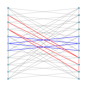
Figure 3: Two perspectives on the graph $G$. In both are highlighted all the squares which contain the vertices 5 and 16 (in blue) and the vertices 7 and 14 (in red). Both drawings emphasize the bipartite division of the vertices, the drawing on the left highlights the distinction (as seen by the different “slopes”) between the blue squares which are in the first component of full support and the red squares which are in the second component of full support. The figure at right is drawn to emphasize the symmetry and to avoid the multiple collinear vertices which hide some of the edges in the graph on the left (for instance those connecting the vertices at the bottom to the ones at the top).

The diagonals of the first square component with full support are the diagonals coming from $G^{\prime}$, and the diagonals of the second square component with full support are the diagonals coming from squares which use some edges from $G^{\prime\prime}$. Note that both sets of diagonals have full support by construction. Also note that every diagonal of a square in $G$ is of one of the two forms noted in the two bullet points above. Since the ones in $G^{\prime}$ and those including an edge of $G^{\prime\prime}$ are distinct, no diagonal in one can be connected in $T_{1}(G)$ to a diagonal from the other. Thus $T_{1}(G)$ has two distinct components both having full support in $G$. ∎

This construction was independently verified by computer and a number of related examples were also generated and checked. We note in particular that a slight variant of the above ideas yield an example in which there are three distinct square components with full support (using 22 vertices on each side instead of 11 and then shifting by 12 instead of 6), and further variations also one to build examples with an even larger number of distinct square components of full support.

2.2.2 Non-monotonicity of connectivity in square percolation

The connectivity properties of the graphs $T_{k}(\Gamma)$ are not monotone under the addition of edges to $\Gamma$. Indeed, adding an edge to $\Gamma$ could have a number of different potential effects. It could create new induced squares in $\Gamma$ (and thus new edges in $T_{1}(\Gamma)$), but it also removes a non-edge (so that $T_{1}(\Gamma)$ loses a vertex and all edges incident with it), which can destroy some induced squares that were in $\Gamma$.

As an example, consider the complete bipartite graph $\Gamma=K_{2,n-2}$ with one part of size $2$ and another of size $n-2$. Clearly, $T_{1}(\Gamma)$ is connected. However if we delete any edge from $\Gamma$, or if we add an edge inside the part of size $2$, then $T_{1}(\Gamma)$ becomes disconnected (and in the later case becomes an empty graph on $\binom{n-2}{2}$ vertices!). This illustrates the sensitivity and non-monotonicity of the connectivity properties we are considering in this paper.

2.3 The extremal bound for thick graphs

We also state here the following useful property of graphs that have a square component with full support, which was first proved in [4, Lemma 5.5], and later greatly generalized so as to encompass all thick graphs in [8, Theorem 1.4].

Proposition 2.4 (Extremal bound for thick graphs [4, 8]).

Let $\Gamma$ be a graph on $n$ vertices such that $T_{1}(\Gamma)$ contains a component $C$ with $\mathrm{supp}(C)=V(\Gamma)$. Then $e(\Gamma)\geq 2n-4$.

2.4 Probabilistic notation and tools

We write $\mathbb{P}$, $\mathbb{E}$ and $\mathrm{Var}$ for probability, expectation and variance respectively. We say that a sequence of events $\mathcal{E}=\mathcal{E}(n)$, $n\in\mathbb{N}$ holds a.a.s. (asymptotically almost surely) if $\lim_{n\rightarrow\infty}\mathbb{P}(\mathcal{E}(n))=1$. Throughout the paper we use standard Landau notation: for functions $f,g:\ \mathbb{N}\rightarrow\mathbb{R}$ we write $f=o(g)$ if $\lim_{n\rightarrow\infty}f(n)/g(n)=0$, $f=O(G)$ if there exists a real constant $C>0$ such that $\limsup_{n\rightarrow\infty}|f(n)/g(n)|\leq C$. We occasionally use $f\ll g$ as a shorthand for $f=o(g)$. We further write $f=\omega(g)$ if $g=o(f)$ and $f=\Omega(g)$ if $g=O(f)$. Finally we write $f=\theta(g)$ if $f=O(g)$ and $f=\Omega(g)$ both hold.

We shall make repeated use of Markov’s inequality: given a non-negative integer-valued random variable $X$, $\mathbb{P}(X>a)\leq\frac{1}{a+1}\mathbb{E}X$ for any integer $a\geq 0$. We shall also use the following standard Chernoff bound, see e.g.  [1, Theorems A.1.11 and A.1.13]:

Proposition 2.5 (Chernoff bound).

Let $X_{1},X_{2},\ldots,X_{n}$ be independent and identically distributed Bernoulli random variables. Set $X=\sum_{i}X_{i}$ and $\mu:=\mathbb{E}X$. Then for any $\delta\in(0,2/3)$,

$$\mathbb{P}(|X-\mu|\geq\delta\mu)\leq 2\exp\left(-\frac{\delta^{2}\mu}{3}\right).$$

Finally, we shall need Janson’s celebrated inequality [26] as well as a large deviation extension of it due to Janson [25], which can be found in the form given below in e.g. [1, Theorem 8.1.1 and 8.7.2]. Given a set $X$ and $q\in[0,1]$, a $q$-random subset $X^{\prime}$ of $X$ is obtained by including each element of $X$ in $X^{\prime}$ with probability $q$, independently of all other elements.

Proposition 2.6 (Janson inequalities).

Let $U$ be a finite set and $U_{q}$ a $q$-random subset of $U$ for some $q\in[0,1]$. Let $\mathcal{F}$ be a family of subsets of $U$, and for every $F\in\mathcal{F}$ let $I_{F}$ be the indicator function of the event $\{F\subseteq U_{q}\}$. Set $I_{\mathcal{F}}=\sum_{F\in\mathcal{F}}I_{F}$, and let $\mu=\mathbb{E}I_{\mathcal{F}}$ and $\Delta=\sum_{F,F^{\prime}\in\mathcal{F}:\ F\cap F^{\prime}\neq\emptyset,\ F\neq F^{\prime}}\mathbb{E}(I_{F}I_{F}^{\prime})$. Then

$$\mathbb{P}\left(I_{\mathcal{F}}=0\right)\leq\exp\left(-\frac{\mu^{2}}{2\Delta}\right) \mathbb{P}\left(I_{\mathcal{F}}=0\right)\leq\exp\left(-\mu+\frac{\Delta}{2}\right).$$ and

Further, for any $\gamma>0$,

$$\mathbb{P}\left(I_{\mathcal{F}}\leq(1-\gamma)\mu\right)\leq\exp\left(-\frac{\gamma^{2}\mu}{2+2(\Delta/\mu)}\right).$$

2.5 Building and connecting giants in square percolation

We shall need two results of Behrstock, Falgas–Ravry and Susse from [5]. The first establishes that for $p$ slightly above the threshold for the emergence of a giant square component, the number of non-edges in somewhat-large square components is concentrated around its mean (which is of order $\Omega(n^{2})$).

Proposition 2.7 (Many edges in large components [5, Corollary 6.3]).

Let $c>\sqrt{\sqrt{6}-2}$ be fixed, and let $C>0$ be an arbitrary constant. Let $\Gamma\sim\mathcal{G}_{n,p}$ and suppose $p=p(n)$ satisfies

$$\frac{\lambda}{\sqrt{n}}\leq p(n)\leq C\sqrt{\frac{\log n}{n}}.$$

Then with probability $1-O(n^{-1})$, the number $N_{v}$ of non-edges $f\in E(\overline{\Gamma})$ that belong to square components of size at least $(\log n)^{4}$ satisfies

$$N_{v}=(1-o(1))\mathbb{E}N_{v}=\Omega(n^{2}).$$

(This was formally stated with $C=5$ in [5, Corollary 6.3], but the proof works for any choice of the constant $C>0$ in the upper bound on $p(n)$.)

The second result concerns vertex-sprinkling; it allows a number of somewhat-large square components to connect up into a giant square component.

Proposition 2.8 (Sprinkling lemma [5, Lemma 6.6]).

Suppose we have a bipartition of $V(\Gamma)$ into $V_{1}\sqcup V_{2}$ such that:

1. $|V_{2}|=\Omega(n)$;

2. there are $\Omega(n^{2})$ pairs from $E(\overline{\Gamma[V_{1}]})$ that lie in components of $T_{1}(\Gamma[V_{1}])$ of size at least $(\log n)^{4}$;

3. $\Omega\left(\frac{1}{\sqrt{n}}\right)\leq p(n)\leq O\left(\left(\frac{\log n}{n}\right)^{\frac{1}{3}}\right)$.

Then the probability that there exists a square component $C$ in $T_{1}(\Gamma)$ containing all the pairs from $E(\overline{\Gamma[V_{1}]})$ that lie in components of $T_{1}(\Gamma[V_{1}])$ of size at least $(\log n)^{4}$ is at least

$$1-\exp\left(-\Omega\left((\log n)^{2}\right)\right).$$

(Formally, this was stated with an upper bound of $p(n)=O\left(\sqrt{(\log n)/n}\right)$, but the proof of the connecting lemma [5, Lemma 6.4], which is the main tool in the proof of [5, Lemma 6.6], carries over when we have the weaker upper bound $p(n)\leq O\left(\sqrt[3]{(\log n)/n}\right)$ without any change, as does the remainder of the proof of [5, Lemma 6.6].)

We shall need an additional result that is somewhat reminiscent of the connecting lemma [5, Lemma 6.4], and is proved in an analogous manner via Janson’s inequality.

Proposition 2.9 (Giant-connecting lemma).

Let $\Gamma~\sim\mathcal{G}_{n,p}$, with $p=p(n)$ satisfying

$$\frac{1}{\sqrt{n}}\ll p(n)\leq 100\left(\frac{\log n}{n}\right)^{\frac{1}{3}}.$$

Let $M=M(n)$ be such that $1\ll M\ll p^{-1}$. Suppose $W_{1}\sqcup W_{2}$ is a partition of $V(\Gamma)$ such that $|W_{1}|=n/M$, and there are $\Omega(n^{2})$ non-edges of $W_{2}$ that lie in the same (giant) component $C_{2}$ of $T_{1}(\Gamma[W_{2}])$. Then the probability that there exists some component $C_{1}$ of $T_{1}(\Gamma[W_{1}])$ of size at least $M$ such that $C_{1}$ and $C_{2}$ are not a subset of the same component in $T_{1}(\Gamma)$ is at most

$$\frac{n^{2}}{M^{3}}\exp\left(-\Omega\left(Mnp^{2}\right)\right).$$

Further, if there exist two distinct components $C_{2}$ and $C_{2}^{\prime}$ of $T_{1}(\Gamma[W_{2}])$ of size $\Omega(n^{2})$, then with probability $1-\exp(-\Omega(n^{2}p^{2}))$ they are a subset of the same component in $T_{1}(\Gamma)$.

Proof.

Let $U$ denote the complete bipartite graph with bipartition $W_{1}\sqcup W_{2}$. Clearly, the collection of edges of $\Gamma$ from $W_{1}$ to $W_{2}$ is distributed as a $p$-random subset of $U$.

Given a component $C_{1}$ of $T_{1}(\Gamma[W_{1}])$ of size at least $M$, there are $\Omega(n^{2}M)$ pairs $\{x_{1}x_{2},y_{1}y_{2}\}$ with $x_{1}x_{2}\in C_{1}$, $y_{1}y_{2}\in C_{2}$. For each such pair, we define $F_{x_{1}x_{2},y_{1}y_{2}}$ to be the event that $x_{i}y_{j}\in E(\Gamma)$ for every $i,j\in[2]$, i.e., that $x_{1}x_{2}y_{1}y_{2}$ induces a square of $\Gamma$ joining $C_{1}$ to $C_{2}$ in $T_{1}(\Gamma)$. The probability of this event is $p^{4}$, and we are thus in a position to apply Janson’s inequality.

We have $\mu=\Omega(n^{2}Mp^{4})$. To compute the parameter $\Delta$, note that $F:=F_{x_{1}x_{2},y_{1}y_{2}}$ and $F^{\prime}:=F_{x^{\prime}_{1}x^{\prime}_{2},y^{\prime}_{1}y^{\prime}_{2}}$ are independent unless $X:=|\{x_{1},x_{2}\}\cap\{x^{\prime}_{1},x^{\prime}_{2}\}|$ and $Y:=|\{y_{1},y_{2}\}\cap\{y^{\prime}_{1},y^{\prime}_{2}\}|$ are both strictly positive. If $(X,Y)=(2,2)$ then $F=F^{\prime}$. Further, note that $\mathbb{E}I_{F}I_{F^{\prime}}$ is equal to $p^{7}$ if $(X,Y)=(1,1)$ and to $p^{6}$ if $(X,Y)=(2,1)$ or $(1,2)$.

Now for $\{x_{1}x_{2},y_{1}y_{2}\}$ fixed we have $O(n)$ ways of picking $y^{\prime}_{1}y^{\prime}_{2}\in C_{2}$ such that $Y=1$ and at most $M$ ways of picking $x^{\prime}_{1}x^{\prime}_{2}\in C_{1}$ such that $X=1$. Going over all possibilities $(X,Y)\in\{(1,1),(2,1),(1,2)\}$, calculating $I_{F}I_{F^{\prime}}$ in each case and using our assumption that $M\ll p^{-1}$, we see that

$$\Delta=O\left(\mu p^{2}n\right).$$

It then follows from Proposition 2.6, Janson’s inequality, together with linearity of expectation and Markov’s inequality that the probability that one of the at most $n^{2}/(2M^{3})$ choices of a square component $C_{1}$ in $T_{1}(\Gamma[W_{1}])$ with size at least $M$ that does not join up to $C_{2}$ in $T_{1}(\Gamma)$ is at most

$$\frac{n^{2}}{2M^{3}}\exp\left(-\Omega\left(\frac{\mu}{p^{2}n}\right)\right)=\frac{n^{2}}{M^{3}}\exp\left(-\Omega\left(Mp^{2}n\right)\right).$$

It remains to show the ‘Further’ part of the proposition. Let $\mathcal{B}$ be the event that there are fewer than $\frac{n^{2}}{4M^{2}}$ non-edges in $\Gamma[W_{1}]$. Applying the Chernoff bound (Proposition 2.5), we have $\mathbb{P}(\mathcal{B})=\exp\left(-\Omega(n^{2}/M^{2})\right)$, which by our bounds on $p$ and $M$ is at most $\exp\left(-\Omega(n^{2}p^{2})\right)$.

Suppose the event $\mathcal{B}$ does not occur. Now, note that there are at most $O(1)$ distinct giant square components in $T_{1}(\Gamma[W_{2}])$. For any such pair of giants $C_{2},C_{2}^{\prime}$ and any $x_{1}x_{2}\in C_{2}$, $y_{1}y_{2}\in C_{2}^{\prime}$ with $\{x_{1},x_{2}\}\cap\{y_{1},y_{2}\}=\emptyset$ and any non-edge $z_{1}z_{2}\in E(\overline{\Gamma[W_{1}]})$, let $F_{x_{1}x_{2},y_{1}y_{2},z_{1}z_{2}}$ be the event that $x_{i}z_{j}$ and $y_{i}z_{j}$ are edges of $\Gamma$ for every $i,j\in[2]$ (and in particular that $C_{2}$ and $C_{2}^{\prime}$ join up in $T_{1}(\Gamma)$ through two induced squares both having $z_{1}z_{2}$ as a diagonal). Clearly the probability of this event is $p^{8}$. Conditional on $\mathcal{B}$ not occurring, there are $\Omega(n^{6}/M^{2})$ such triples $x_{1}x_{2},y_{1}y_{2},z_{1}z_{2}$. Here again we can apply Janson’s inequality with parameters $\mu=\Omega(p^{8}n^{6}/M^{2})$ and $\Delta=O\left(\mu n^{3}p^{6}/M\right)$ to deduce that the probability that $C_{2}^{\prime}$ and $C_{2}$ fail to connect in $T_{1}(\Gamma)$ through a $F_{x_{1}x_{2},y_{1}y_{2},z_{1}z_{2}}$-event when we reveal the edges from $W_{1}$ to $W_{2}$ is at most

$$\exp\left(-\mu^{2}/2\Delta\right)=\exp(-\Omega(n^{3}p^{3})),$$

where in the last inequality we have used our assumption that $M\ll p^{-1}$. Since as noted above there can be only $O(1)$ pairs of distinct giants $C_{2},C_{2}^{\prime}$ in $T_{1}(\Gamma[W_{2}])$, it follows from Markov’s inequality that the probability any two of them fail to join up in $T_{1}(\Gamma[W])$ is at most $\mathbb{P}(\mathcal{B})+O(1)\cdot\exp(-\Omega(n^{3}p^{3}))=\exp(-\Omega(n^{2}p^{2}))$, as claimed. ∎

3 Connectivity in square percolation

3.1 Proof outline

Our proof of Susse’s conjecture on the location of the connectivity threshold for $S(\Gamma)$ (and $T_{1}(\Gamma)$), $\Gamma\sim\mathcal{G}_{n,p}$ is structured as follows.

We first show that for ‘large’ $p$ (which for us means $p=\Omega\left((\log(n)/n)^{\frac{1}{3}}\right)$, $T_{1}(\Gamma)$ is connected (Proposition 3.2). We then concentrate on values of $p=p(n)$ which are not ‘large’, but which are a little above the threshold for the emergence of a giant component in $T_{1}(\Gamma)$ (which occurs at $p\approx\sqrt{\sqrt{6}-2}/\sqrt{n}$). For $p$ in this range we prove Theorem 1.4, showing that a.a.s. the giant square component is unique and that all other square components are small, with size $O((\log n)^{2})$. For this part of the argument, we rely on a partial converse to Propositions 2.4 (Lemma 3.5), the tools from [5] we discussed in Section 2, and somewhat intricate partitioning arguments.

Finally, we use Lemma 3.5, Proposition 2.4 and Janson’s inequality to rule out the existence of small square components of size $O((\log n)^{2})$ for $p$ just above Susse’s conjectured connectivity threshold, thereby completing the proof of Theorem 1.1.

3.2 One square component to rule them all: proof of Theorem 1.4

We begin with a series of propositions showing that for large $p$, the a.a.s. existence of a unique giant component is essentially trivial.

Proposition 3.1.

Let $\Gamma\sim\mathcal{G}_{n,p}$. If $p=p(n)$ satisfies

$$100\left(\frac{\log n}{n}\right)^{\frac{1}{4}}\leq p(n)\leq 1-\omega(n^{-2}),$$

then a.a.s. $T_{1}(\Gamma)$ has diameter at most two and in particular is connected.

Proof.

Case 1: $\mathbf{1-p\geq 100/n}$. Let $x_{1}x_{2}$ and $y_{1}y_{2}$ be distinct (but not necessarily disjoint) pairs of vertices from $V(\Gamma)$; the size of the common neighbourhood of $\{x_{1},x_{2},y_{1},y_{2}\}$ in $\Gamma$ stochastically dominates a $\mathrm{Binomial}(n-4,p^{4})$ random variable. Applying a Chernoff bound (Proposition 2.5) to bound the probability of the pairs having fewer than $p^{4}n/2$ neighbours in common and taking the union bound over all such pairs, we see that for $p\geq 100\left(\frac{\log n}{n}\right)^{\frac{1}{4}}$, a.a.s. all distinct pairs $x_{1}x_{2}$, $y_{1}y_{2}$ from $V(\Gamma)^{(2)}$ have at least $\frac{p^{4}n}{2}$ neighbours in common.

Further, using the bound $\binom{n}{m}\leq\left(\frac{en}{m}\right)^{m}$, we have that the expected number of $m$–cliques in $\Gamma$ is $\binom{n}{m}p^{\binom{m}{2}}\leq\left(\frac{en}{m}p^{\frac{m-1}{2}}\right)^{m}$. For $m=\lceil\frac{p^{4}n}{4}\rceil$ and $p\leq 1-\frac{100}{n}$, the value of this expectation is $o(1)$, whence by Markov’s inequality a.a.s. $\Gamma$ contains no such clique. In particular, a.a.s. any $p^{4}n/2$–set in $\Gamma$ contains at least one non-edge.

It follows from the two previous paragraphs that a.a.s. for any pair of distinct non-edges $x_{1}x_{2}$, $y_{1}y_{2}$ from $V(\Gamma)^{(2)}\setminus E(\Gamma)$ there exists a non-edge $z_{1}z_{2}\in E(\overline{\Gamma})$ with $z_{1},z_{2}$ lying in the common neighbourhood of $\{x_{1},x_{2},y_{1},y_{2}\}$, whence $x_{1}x_{2}$ and $y_{1}y_{2}$ are connected by a path of length at most two in $T_{1}(\Gamma)$. This establishes the proposition in this case.

Case 2: $\mathbf{\omega(n^{-2})\leq 1-p\leq 100/n}$. By classical results on the connectivity threshold for the Erdős–Rényi random graph model $\mathcal{G}_{n,1-p}$ [19], the complement graph $\overline{\Gamma}\sim\mathcal{G}_{n,1-p}$ of $\Gamma$ is a.a.s. not connected. In particular non-edges of $\Gamma$ from distinct components of $\overline{\Gamma}$ are joined by a square in $\Gamma$. Since for $\omega(n^{-2})\leq 1-p(n)\leq\frac{100}{n}$ the graph $\overline{\Gamma}$ a.a.s. contains at least two distinct non-trivial components (by e.g., a standard second moment argument), it follows that for $p$ in this range $T_{1}(\Gamma)$ again has a.a.s. diameter at most two.∎

Proposition 3.2.

Let $\Gamma\sim\mathcal{G}_{n,p}$, and let $\varepsilon>0$ be fixed. If $p=p(n)$ satisfies

$$100\left(\frac{\log n}{n}\right)^{\frac{1}{3}}\leq p(n)\leq 100\left(\log(n)/n\right)^{\frac{1}{4}}$$

then a.a.s. $T_{1}(\Gamma)$ is connected.

Proof.

We argue similarly to Case 1 in Proposition 3.1. Since the distribution of the number of neighbours of a triple of vertices is $\mathrm{Binomial}(n-3,p^{3})$, applying a Chernoff bound (Proposition 2.5) and taking the union over all such triples, we see that for $p\geq 100\left(\log(n)/n\right)^{\frac{1}{3}}$ the following holds:

1. a.a.s. every triple of vertices in $\Gamma$ has at least $p^{3}n/2$ common neighbours.

Further, the expected number of cliques of size $m=\lceil p^{3}n/2\rceil$ is at most $\left(\frac{ne}{m}p^{\frac{m-1}{2}}\right)^{m}=o(1)$ for $p\leq 100\left(\log(n)/n\right)^{\frac{1}{4}}$. Thus, we have that

1. a.a.s. every set of $p^{3}n/2$ vertices in $\Gamma$ must contain at least one non-edge of $\Gamma$.

It follows from the two facts (a) and (b) that

1. a.a.s.  for any pair of intersecting non-edges $xy,yz\in E(\overline{\Gamma})$, $xy,yz$ belong to the same square component.

Now, for $p$ in the range we are considering, classical results of Erdős and Rényi [19] imply that

1. a.a.s. $\overline{\Gamma}\sim\mathcal{G}_{n,1-p}$ is connected.

It follows from (c) and (d) that $T_{1}(\Gamma)$ is a.a.s. connected. ∎

By a Chernoff bound, for $p(n)\leq 1-\omega(n^{-2})$ we have that with probability $1-\exp(-\Omega(n^{2}(1-p)))=1-o(1)$ that there are $\Omega(n^{2}(1-p))=\omega(1)$ non-edges in $\Gamma$, each of which is a vertex of $T_{1}(\Gamma)$. It thus follows from Propositions 3.1 and 3.2 that for $p(n)$ between $100(\log(n)/n)^{\frac{1}{3}}$ and $1-\omega(n^{-2})$, a.a.s. there exists a unique component in $T_{1}(\Gamma)$ of order $\Omega(n^{2}(1-p))$, proving Theorem 1.4 in that range.

In the remainder of this subsection, we turn therefore our attention to the range

$$p(n)\in R=R(n):=[C\sqrt{\frac{\log\log n}{n}},100(\log(n)/n)^{\frac{1}{3}}],$$

where $C>0$ is a large constant to be specified later. We first establish a simple proposition whose purpose is to extend upwards the range of $p$ for which we can guarantee that many non-edges are in ‘somewhat large’ square components from that given in Proposition 2.7.

Proposition 3.3.

Suppose $p(n)$ satisfies $50\sqrt{\log(n)/n}\leq p\leq 100\left(\log(n)/n\right)^{\frac{1}{3}}$. Then with probability $1-O(n^{-1})$, every non-edge of $\Gamma$ belongs to a square component of size at least $(\log n)^{4}$.

Proof.

The expected number of complete subgraphs on $8$ vertices contained in $\Gamma$ is $\binom{n}{8}p^{\binom{8}{2}}=O(n^{8}p^{28})$, which for $p\leq n^{-\frac{1}{3}+o(1)}$ is $o(n^{-1})$. Thus by Markov’s inequality, the event $\mathcal{B}$ that $\Gamma$ contains a complete subgraph on $8$ vertices has probability at most $o(n^{-1})$.

Consider a pair of vertices $v,v^{\prime}$ from $V(\Gamma)$ with $vv^{\prime}\notin E(\Gamma)$. By a Chernoff bound (Proposition 2.5), with probability at least $1-2\exp\left(-(\frac{1}{12}+o(1))p^{2}n\right)=1-O(n^{-3})$, the set $X$ of common neighbours of $v$ and $v^{\prime}$ has size at least $\frac{1}{2}p^{2}n$ and at most $\frac{3}{2}p^{2}n$. If $\mathcal{B}$ does not occur, then $\Gamma[X]$ does not contain any complete graph on $8$ vertices, whence by Turán’s theorem [32] it contains at most $\left(1-\frac{1}{7}+o(1)\right)\binom{|X|}{2}$ edges. In particular, there is a set $C=X^{(2)}\cap E(\overline{\Gamma})$ of a least $(\frac{1}{7}-o(1))\binom{p^{2}n/2}{2}>\frac{1}{64}p^{4}n^{2}$ non-edges in $\Gamma[X]$, all of which lie inside the same square component as $vv^{\prime}$.

Case 1: $\mathbf{p\geq 4\log n/\sqrt{n}}$. Taking a union bound over the $\binom{n}{2}$ pairs $vv^{\prime}$ from $V(\Gamma)^{(2)}$, the argument above shows that with probability $1-\mathbb{P}(\mathcal{B})-\binom{n}{2}\cdot O(n^{-3})=1-O(n^{-1})$, every pair $vv^{\prime}\in E(\overline{\Gamma})$ is in a component of $T_{1}(\Gamma)$ of size at least $(\log n)^{4}$.

Case 2: $\mathbf{p\leq 4\log n/\sqrt{n}}$. Suppose $\mathcal{B}$ does not occur. With $X$ and $C$ as above, and $C$ in particular of size at least $\frac{1}{64}p^{4}n^{2}>10000(\log n)^{2}$, there must exist a perfect matching $e_{1},e_{2},\ldots,e_{m}$ of $m:=\lceil 100\log n\rceil$ non-edges of $\Gamma$ inside $X$ (i.e., $m$ pairwise disjoint non-edges). We use these non-edges to explore the square component containing $vv^{\prime}$. For $1\leq t\leq m$, do the following: set $X_{t}$ to be the set of vertices in $V(\Gamma)\setminus(X\cup\{v,v^{\prime}\})$ sending edges to both vertices in $e_{t}=v_{t}v^{\prime}_{t}$, and let $C_{t}:=X_{t}^{(2)}\cap E(\overline{\Gamma})$. If $X_{t}$ has size less than $\frac{1}{2}p^{2}n$ or more than $\frac{3}{2}p^{2}n$, terminate the process. Else it follows from Turán’s theorem, just as in the analysis about Case $1$, that $C_{t}$ has size at least $10000(\log n)^{2}$ and contains a collection $e_{(t-1)m+1},\ldots,e_{tm}$ of $m$ non-edges in $X_{t}$ forming a perfect matching. Add $C_{t}$ to $C$ and $X_{t}$ to $X$. Then if $t\geq(\log n)^{2}$, terminate the process, otherwise move to step $t+1$ of our iterative exploration.

We claim that either $\mathcal{B}$ occurs or with probability $1-O(n^{-3})$ the process ends with $t=\lceil(\log n)^{2}\rceil$ and we have $\frac{1}{2}p^{2}n\leq|X_{t}|\leq\frac{3}{2}p^{2}n$ at each time step $t$: $1\leq t\leq(\log n)^{2}$. Note that if this is the case then $C$ at the end of the process has size at least $(\log n)^{4}$, and is part of the same component as $vv^{\prime}$ in $T_{1}(\Gamma)$. Taking a union bound over all pairs $vv^{\prime}$, our claim would thus imply that with probability $1-\mathbb{P}(\mathcal{B})-\binom{n}{2}\cdot O(n^{-3})=1-O(n^{-1})$, every pair $vv^{\prime}\in E(\overline{\Gamma})$ is in a component of $T_{1}(\Gamma)$ of size at least $(\log n)^{4}$, as desired.

Let us therefore prove our claim. Note first of all that at each time step $t<(\log n)^{2}$ before the process terminates we have $V(\Gamma)\setminus(X\cup\{v,v^{\prime}\})>n-2t(\log n)^{2}p^{2}n=(1-o(1))n$. By a Chernoff bound, with probability $1-2\exp\left(-(\frac{1}{12}+o(1))p^{2}n\right)=1-O\left(n^{-4}\right)$, we have that $X_{t}\in[\frac{p^{2}n}{2},\frac{3p^{2}n}{2}]$. Thus as claimed either $\mathcal{B}$ occurs or with probability $1-(\log n)^{2}O(n^{-4})=1-O(n^{-4})$ the process ends with $t=\lceil(\log n)^{2}$ and $\frac{1}{2}p^{2}n\leq|X_{t}|\leq\frac{3}{2}p^{2}n$ holding at each time step $t$: $1\leq t\leq(\log n)^{2}$. ∎

Corollary 3.4.

Fix a subset $V^{\prime}\subseteq V(\Gamma)$ with $|V^{\prime}|=\left(1-o(1)\right)n$, let $p=p(n)\in R$. Then with probability $1-O(n^{-1})$, there exists a giant square component in $T_{1}(\Gamma[V^{\prime}])$ of size $\Omega(n^{2})$.

Proof.

Fix $\delta>0$, and partition the set $V^{\prime}$ as $V^{\prime}=V_{1}\sqcup V_{2}$, where $|V_{2}|=(\delta+o(1))n$ and $|V_{1}|=(1-\delta-o(1))n$. By Propositions 2.7 and 3.3, we have that with probability $1-O(n^{-1})$ there are $\Omega(n^{2})$ non-edges of $\Gamma[V_{1}]$ that lie in square components of $T_{1}(\Gamma[V_{1}])$ of size at least $(\log n)^{4}$. The corollary is then immediate from the sprinkling lemma, Proposition 2.8. ∎

The last tool we need is the following partial converse to Proposition 2.4, giving a lower bound on the number of non-edges in a graph $\Gamma$ that has a square component of full support.

Lemma 3.5.

Suppose $\Gamma$ is a graph on $m\geq 4$ vertices, and that $C$ is a square component of $\Gamma$ with full support, $\mathrm{supp}(C)=V(\Gamma)$. Then $|C|\geq m/2$.

Proof.

By definition, every vertex $u\in V(\Gamma)=\mathrm{supp}(C)$ belongs to a non-edge $uv\in E(\overline{\Gamma})$ with $uv\in C$. By double-counting, $C$ must have size at least $m/2$. ∎

With these results in hand, we are now ready to prove Theorem 1.4 for the remaining range of $p$, $p\in R$.

Proof of Theorem 1.4.

Let $C>0$ be a sufficient large constant, and let $p=p(n)$ satisfy

$$\frac{C\sqrt{\log\log n}}{\sqrt{n}}\leq p\leq 100\left(\frac{\log n}{n}\right)^{\frac{1}{3}}.$$

Let $\Gamma\sim\mathcal{G}_{n,p}$ and write $V$ for $V(\Gamma)$. Let $M=\lfloor\frac{\log n}{8\log\log n}\rfloor$. Take a balanced partition $V=\sqcup_{i=1}^{2M^{2}}V_{i}$ of the vertex set of $\Gamma$ into $2M^{2}$ parts. Given a subset $S$ of $[2M^{2}]$, we denote by $V_{S}:=\bigcup_{i\in S}V_{i}$ the union of all parts $V_{i}$ with $i\in S$.

Given any subset $S\in[2M^{2}]^{(2M)}$, let $E_{S}$ be the event that there is a giant square component $C$ inside $T_{1}(\Gamma[V\setminus V_{S}])$ containing $\Omega(n^{2})$ non-edges of $\Gamma$, and further that every square component $C^{\prime}$ of $T_{1}(\Gamma[V_{S}])$ of size at least $M$ joins up to (every such giant) $C$ in $T_{1}(\Gamma)$. We claim that $E_{S}$ occurs with very high probability.

Claim 3.6.

For every $S\in[2M^{2}]^{(2M)}$, we have $\mathbb{P}(\overline{E_{S}})=o\left({\binom{2M^{2}}{2M}}^{-1}\right)$.

Proof.

Since $|V\setminus V_{S}|=(1-\frac{1}{M}+o(1))n=(1+o(1))n$, it follows from Corollary 3.4 that with probability $1-O(n^{-1})$ there exists a giant square component $C$ inside $T_{1}(\Gamma[V\setminus V_{S}])$. If such a giant exists, Proposition 2.9 tells us there is a probability of at most $n^{2}M^{-3}\exp\left(-\Omega(Mnp^{2})\right)$ that some component of size $M$ in $T_{1}(\Gamma[V_{S}])$ fails to connect up to it in $T_{1}(\Gamma)$. Picking our constant $C$ sufficiently large, we have that for $p\geq C\sqrt{\log\log(n)/n}$ this probability is $O(n^{-1})$. Putting it all together, the probability of $E_{S}$ is $1-O(n^{-1})=1-o\left({\binom{2M^{2}}{2M}}^{-1}\right)$, proving the lemma. It is here that our choice of $M$ comes in, as it ensures that ${2eM}^{4M}=\exp\left(\left(\frac{1}{2}+o(1)\right)\log n\right)$ so that $\binom{2M^{2}}{M}^{2}\leq\left(\frac{2eM^{2}}{M}\right)^{2M}=o(n)$. ∎

Further, given subsets $S,S^{\prime}\in[2M^{2}]^{(2M)}$ with $|S\cap S^{\prime}|=2M-1$, let $E_{S,S^{\prime}}$ be the event that for every pair of components $C$ in $T_{1}(\Gamma[V\setminus V_{S}])$ and $C^{\prime}$ in $T_{1}(\Gamma[V\setminus V_{S^{\prime}}])$ such that $C,C^{\prime}$ both have size $\Omega(n^{2})$, $C$ and $C^{\prime}$ join up in $T_{1}(\Gamma)$. Again, we claim that this event $E_{S,S^{\prime}}$ occurs with very high probability.

Claim 3.7.

For every $S,S^{\prime}\in[2M^{2}]^{(2M)}$ with $|S\cap S^{\prime}|=2M-1$, $\mathbb{P}(\overline{E_{S,S^{\prime}}})=o\left({\binom{2M^{2}}{2M}}^{-2}\right)$.

Proof.

Our condition on $M$ ensures $|V_{S}\cap V_{S^{\prime}}|=(1+o(1))\frac{n}{2M^{2}}(2M-1)=(1+o(1))\frac{n}{M}=(1+o(1))\frac{8n\log\log n}{\log n}$ satisfies $1\ll M\ll p^{-1}$. By Corollary 3.4, with probability $1-O(n^{-1})$ there exists a square component in $\Gamma[V\setminus V_{S}\cap V_{S^{\prime}}]$ of size $\Omega(n^{2})$. We can thus apply the ‘further’ part of Propositions 2.9 to deduce that with probability $1-O(n^{-1})-\exp\left(-\Omega(n^{2}p^{2})\right)=1-o\left({\binom{2M^{2}}{2M}}^{-2}\right)$ every pair of square components of size $\Omega(n^{2})$ from $\Gamma[V\setminus(V_{S}\cap V_{S^{\prime}})]$ join up in $T_{1}(\Gamma)$. ∎

We are now ready to complete the proof of Theorem 1.4. Applying Claim 3.6 and Markov’s inequality, we see that a.a.s. the event $E_{S}$ occurs for every subset $S\in[2M^{2}]^{(2M)}$. Further, by Claim 3.7 and Markov’s inequality, a.a.s the event $E_{S,S^{\prime}}$ occurs for every pair of subsets $S,S^{\prime}\in[2M^{2}]^{(2M)}$ with $|S\cap S^{\prime}|=2M-1$. We may therefore in the remainder of the proof condition on the a.a.s. event $\mathcal{E}:=\left(\bigcap_{S\in[2M^{2}]^{(2M)}}E_{S}\right)\cap\left(\bigcap_{S,S^{\prime}\in[2M^{2}]^{(2M)}:\ |S\cap S^{\prime}|=2M-1}E_{S,S^{\prime}}\right)$.

Observe that if $C$ is a component in $T_{1}(\Gamma)$ of size at least $\binom{2M}{2}$, then the support of $C$ has size at least $2M$, and by [4, Lemma 5.5], there must be a $2M$–set $X\subseteq V$ and a subset $C_{X}\subseteq C\cap X^{(2)}$ such that $C_{X}$ is a square component in $T_{1}(\Gamma[X])$ with full support. By Lemma 3.5, we must have that $|C_{X}|\geq M$.

Now, $X$ meets at most $2M$ of the parts $V_{i}$, so there exists a set $S\in[2M^{2}]^{(2M)}$ such that $X\subseteq V_{S}$. Since $E_{S}$ holds, we have that $C_{X}$ joins up in $T_{1}(\Gamma)$ to every giant ($\Omega(n^{2})$-sized) component $C$ of $T_{1}(\Gamma[V\setminus V_{S}])$. Further, since $\bigcap_{S,S^{\prime}}E_{S,S^{\prime}}$ holds, we have that for every $S,S^{\prime}\in[2M^{2}]^{(2M)}$ and every pair of giant components $C$ in $T_{1}(\Gamma[V\setminus V_{S}])$ and $C^{\prime}$ in $T_{1}(\Gamma[V\setminus V_{S^{\prime}}])$, $C$ and $C^{\prime}$ join up to the same square component in $T_{1}(\Gamma)$ (since there exists a finite sequence $S_{0}=S,S_{1},S_{2},\ldots,S_{\ell}=S^{\prime}$ with $S_{i}\in[2M^{2}]^{(2M)}$, $|S_{i}\cap S_{i+1}|=2M-1$ and $E_{S_{i},S_{i+1}}$ occurring for every $i\geq 0$, and since by $E_{S_{i}}$ each of the $T_{1}(\Gamma[V\setminus V_{S_{i}}])$ contains a giant component).

It follows that there exists a unique component in $T_{1}(\Gamma)$ of size greater than $\binom{2M}{2}\geq\frac{1}{33}\left(\frac{\log n}{\log\log n}\right)^{2}$, and this component has size $\Omega(n^{2})$ (since $E_{S}$ holds), proving the theorem. ∎

3.3 The connectivity threshold in square percolation

Proof of Theorem 1.1.

Part (i) follows from the work of Susse [31, Corollary 3.8], who proved that for $n^{-1}\ll p\leq(1-\varepsilon)\sqrt{\log n/n}$, a.a.s. $T_{1}(\Gamma)$ contains isolated squares: induced copies of the $4$–cycle $C_{4}$ not sharing a diagonal with any other induced copy of $C_{4}$. Each of these isolated squares corresponds to an isolated edge in $T_{1}(\Gamma)$, and thus an isolated vertex in $S(\Gamma)$. The a.a.s existence of these isolated vertices implies that $S(\Gamma)$ is a.a.s. not connected for $p$ in this range.

Part (iii) is proved using a similar second-moment argument. Suppose $p\leq\sqrt{2-\varepsilon}\sqrt{\log n/n}$. Then we claim that a.a.s. there are non-edges of $\Gamma$ that are not contained in any induced square. Such non-edges correspond to isolated vertices of $T_{1}(\Gamma)$, and ensure the latter graph is not connected. It is therefore enough to prove our claim, which we now do.

Given a pair $e\in V(\Gamma)^{(2)}$, let $X_{e}$ be the indicator function of the event that $e$ is a non-edge of $\Gamma$ whose endpoints have no neighbour in common. Observe that if $X_{e}=1$, then certainly $e$ is not contained in any induced square of $\Gamma$. Set $X=\sum_{e}X_{e}$. Straightforward calculations then give

$$\mathbb{E}X=\binom{n}{2}(1-p)(1-p^{2})^{n-2}=\left(\frac{1}{2}+o(1)\right)n^{2}e^{-p^{2}n}\geq\left(\frac{1}{2}+o(1)\right)n^{\varepsilon},$$

while

$$\mathbb{E}(X^{2}) =\binom{n}{2}(1-p)^{2}\left((1-p^{2})^{n-2}+2(n-2)(1-2p^{2}+p^{3})^{n-3}+\binom{n-2}{2}(1-p^{2})^{2(n-4)}(1-p^{4})\right)$$

$$=\left(\mathbb{E}X\right)^{2}(1+o(1)).$$

Thus $\mathrm{Var}(X)=o\left(\left(\mathbb{E}X\right)^{2}\right)$, and it follows immediately from Chebyshev’s inequality that a.a.s. $X=(1+o(1))\mathbb{E}X\gg 1$. Thus a.a.s. for $p\leq\sqrt{2-\varepsilon}\sqrt{\log n/n}$, $T_{1}(\Gamma)$ contains isolated vertices and is not connected.

For Part (ii), consider $p=p(n)\geq(1+\varepsilon)\sqrt{\log n}/\sqrt{n}$. By Proposition 3.2, we may assume that $p=p(n)\leq 100\left(\log(n)/n\right)^{\frac{1}{3}}$. Further, by Theorem 1.4, for $p$ in this range we know that a.a.s.  there exists a unique square component of size at least $(\log n)^{2}$. Thus all that remains to be shown is that a.a.s. $T_{1}(\Gamma)$ contains no smaller non-trivial component, i.e., that $T_{1}(\Gamma)$ consists of a giant component together with a collection of isolated vertices (corresponding to non-edges of $\Gamma$ not belonging to any induced square of $\Gamma$).

For $k\geq 4$ and a $k$–set $S\subseteq V(\Gamma)$, let $X_{S}$ be the indicator function of the event that there exists a connected component $C$ of $T_{1}(\Gamma)$ with support $\mathrm{supp}(C)=S$. Note that every non-trivial connected component of $T_{1}(\Gamma)$ must have support of size at least $4$, by definition. Clearly for $X_{S}$ to be non-zero, we must have that $\Gamma[S]$ contains at least $2k-4$ edges (by Proposition 2.4).

Further, suppose $C$ is a square component with support exactly $S$. Then for every non-edge $f=\{x_{1},x_{2}\}\in\overline{\Gamma}[S]$ belonging to $C$, every neighbour $f^{\prime}=\{y_{1},y_{2}\}$ of $f$ in $T_{1}(\Gamma)$ and every vertex $v\in V(\Gamma)\setminus S$ sending edges to both of the endpoints of $f$, $v$ must also send edges to both of the endpoints of $f^{\prime}$. Indeed, suppose $vx_{1},vx_{2}$ are edges in $\Gamma$ but $vy_{i}$ is not. Then the $4$–set $\{vx_{1}x_{2}y_{i}\}$ induces a square in $\Gamma$ connecting $f$ to $vy_{i}$ in $T_{1}(\Gamma)$, contradicting the fact that $v\notin S=\mathrm{supp}(C)$. Since $X$ has full support on $S$, this implies that any vertex $v\in V(\Gamma)\setminus S$ sending edges to both endpoints of $f$ must in fact send edges to every vertex of $S$ (indeed for any $z\in S$, there is a sequence of non-edges $f_{0}=f$, $F_{1},f_{2},\ldots,f_{t}$ such that for each $i$ $f_{i}\cup f_{i+1}$ induces a square in $\Gamma[S]$ and $z\in f_{t}$).

By Lemma 3.5, any square component $C$ with $\mathrm{supp}(C)=S$ must contain a set $L=\{f_{1},f_{2}$, $\ldots f_{\lceil k/2\rceil}\}$ of at least $k/2$ non-edges in $\Gamma[S]$. Thus the discussion from the previous two paragraphs tells us that if $X_{S}>0$ then all of the following must hold:

1. $|S|=k\geq 4$;

2. $\Gamma[S]$ contains a least $2k-4$ edges;

3. there is a set $L\subseteq S^{(2)}$ of $\lceil k/2\rceil$ distinct pairs of vertices from $S$ such that for every vertex $v\in V(\Gamma)\setminus S$, either $v$ sends edges to all of $S$ or for every $f\in L$, at least one of the endpoints of $f$ does not receive an edge from $v$.

We shall use this information to bound the probability that $X_{S}>0$. Fix a $k$–set $S$, and an arbitrary $\lceil k/2\rceil$–set $L\subseteq S^{(2)}$. Observe that for any $v\in V(\Gamma)\setminus S$, the events $\left(E_{v,f}\right)_{f\in L}$ that $v$ sends edges to both endpoints of $f\in L$ are positively correlated $\mathrm{Bernoulli}(p^{2})$ random variable. Further for $f_{1}\neq f_{2}$, the probability of $E_{v,f_{1}}\cap E_{v,f_{2}}$ is $p^{3}$ if $f_{1}\cap f_{2}\neq\emptyset$ and $p^{4}$ otherwise. We may thus apply Janson’s inequality with $\mu=|L|p^{4}$ and $\Delta\leq 2\binom{|L}{2}p^{3}$ to deduce that

$$\mathbb{P}\left(\bigcap_{f\in L}\overline{E_{v,f}}\right)\leq e^{-\frac{k}{2}p^{2}+\frac{k^{2}}{8}p^{3}}.$$ (3.1)

Now write $\mathcal{A}_{v,L}$ for the event that either (i) $\left(\bigcap_{f\in L}\overline{E_{v,f}}\right)$ occurs or (ii) $v$ sends an edge to every vertex in $S$. Note that for any choice of $L$, the events $\left(\mathcal{A}_{v,L}\right)_{v\in V(\Gamma)\setminus S}$ are mutually independent, and are independent of the state of edges inside $\Gamma[S]$. Noting for $p$ in our range and $k\geq 4$ we have $p^{k}e^{\frac{k}{2}p^{2}}\leq p^{4}e^{2p^{2}}=o(n^{-1})$, it follows from this independence, inequality (3.1), conditions (a)–(c) above, our bounds on $p$ and standard bounds for binomial coefficients that for any $k$ with $4\leq k\leq(\log n)^{2}$ and any $k$–set $S$,

$$\mathbb{P}(X_{S}=1) \leq\mathbb{P}\left(|E(\Gamma[S])|\geq 2k-4\right)\left(\sum_{L\subseteq S^{(2)}:\ |L|=\lceil k/2\rceil}\quad\prod_{v\in V(\Gamma)\setminus S}\mathbb{P}\left(\mathcal{A}_{v,L}\right)\right)$$

$$\leq\binom{\binom{k}{2}}{2k-4}p^{2k-4}\binom{\binom{k}{2}}{\lceil k/2\rceil}\left(p^{k}+e^{-\frac{k}{2}p^{2}+\frac{k^{2}}{8}p^{3}}\right)^{n-k}\leq(1+o(1))(ek)^{\frac{5k}{2}}p^{2k-4}e^{-\frac{k}{2}np^{2}(1-o(1))}.$$

Setting $X_{k}:=\sum_{S\in V(\Gamma)^{(k)}}X_{S}$ and using linearity of expectation, we can exploit the inequality above to bound the expected number of number of square components of $T_{1}(\Gamma)$ with support of size $k$. Given $k$ with $4\leq k\leq(\log n)^{2}$ and a fixed $k$–set $S$, we have

$$\mathbb{E}(X_{k})\leq\binom{n}{k}\mathbb{E}(X_{S})<\left(\frac{en}{k}(ek)^{\frac{5}{2}}p^{2}e^{-\frac{p^{2}n(1+o(1))}{2}}\right)^{k}p^{-4}\leq o\left(\frac{(\log n)^{5k-2}}{n^{\frac{(k-4)+k\varepsilon}{2}}}\right),$$

with the first inequality coming from elementary bound $\binom{n}{k}\leq\left(\frac{en}{k}\right)^{k}$ on the binomial coefficient $\binom{n}{k}$, and the second one from the monotonicity of $x\mapsto xe^{-x}$ in $[1,+\infty)$, our upper bound on $k$ (namely $k\leq(\log n)^{2}$), and our lower bound on $p$ (namely$p\geq(1+\varepsilon)\sqrt{\log n}/\sqrt{n}$). Applying Markov’s inequality and linearity of expectation, this implies that

$$\mathbb{P}\left(\sum_{k=4}^{(\log n)^{2}}X_{k}>0\right)\leq\sum_{k=4}^{(\log n)^{2}}\mathbb{E}X_{k}=O\left(\frac{(\log n)^{20}}{n^{4\varepsilon}}\right)=o(1),$$

and thus a.a.s. there is no square component with support of size between $4$ (the smallest possible size) and $(\log n)^{2}$. By Theorem 1.4 we know that a.a.s.  $X_{n}=1$ and $X_{k}=0$ for $k\in[(\log n)^{2},n-1]$. Thus there is an a.a.s. unique non-trivial square component, and $S(\Gamma)$ is a.a.s. connected as required.

Part (iv) follows directly from Part (iii) and Markov’s inequality: for $p=p(n)$ satisfying $100\left(\log(n)/n\right)^{\frac{1}{3}}\leq p\leq 1-\omega(n^{-2})$, we showed in Proposition 3.2 that $T_{1}(\Gamma)$ is a.a.s. connected. Further by Part (iii) established above, we know that for $\sqrt{2+\varepsilon}\sqrt{\log(n)/n}\leq p(n)\leq 100\left(\log(n)/n\right)^{\frac{1}{3}}$, there is an a.a.s. unique non-trivial component in $T_{1}(\Gamma)$. Thus all we need to rule out is the presence of isolated vertices for $p$ in that range, i.e., the existence of ‘bad’ non-edges of $\Gamma$ that are not contained in any induced square of $\Gamma$. Given $e\in V(\Gamma)^{(2)}$, let $X_{e}$ denote the indicator function of the event that $e$ is a non-edge and that the joint neighbourhood of the endpoints of $e$ forms a clique. Set $X=\sum_{e}X_{e}$, so that $X$ is precisely the number of ‘bad’ non-edges of $\Gamma$. Then by Markov’s inequality and linearity of expectation, our bounds on $p$ as well as the facts that $x\mapsto(1+x+x^{2}+x^{3})e^{-x}$ is monotonous decreasing when $x\geq 3$ and that $np^{\frac{9}{2}}=o((\log n)^{2}n^{-\frac{1}{2}})$, we have that

$$\mathbb{P}\left(X>0\right)\leq\mathbb{E}X \leq\binom{n}{2}(1-p)\sum_{i=0}^{n-2}\binom{n-2}{i}p^{2i}(1-p^{2})^{n-2-i}p^{\binom{i}{2}}$$

$$<n^{2}\left((1+np^{2}+n^{2}p^{5}+n^{3}p^{9}+n^{4}p^{14}+n^{5}p^{20})e^{-p^{2}(n-7)}+\sum_{i\geq 6}\left(np^{\frac{i+3}{2}}\right)^{i}\right)$$

$$=O\left(n^{-\varepsilon}\log n\right)=o(1).$$

Thus a.a.s. $X=0$ and $T_{1}(\Gamma)$ is connected. ∎

3.4 Implications for the geometry of the random RACG

Let $\Gamma$ be any graph. Fioravanti, Levcovitz and Sageev [20] introduced the following notion of a bonded square: an induced square $X$ in $\Gamma$ is bonded if there exists an induced square $X^{\prime}$ in $\Gamma$ such that $X$ and $X^{\prime}$ have exactly three vertices in common. In other words, an induced square with diagonals $f$ and $f^{\prime}$ is bonded if and only if there exists some vertex $v\notin f\cup f^{\prime}$ sending edges to both endpoints of exactly one of $f$ and $f^{\prime}$ (and thus sending at least one non-edge to the other diagonal).

As one of their main results, Fioravanti, Levcovitz and Sageev established in [20, Corollary C] that if every square in a graph $\Gamma$ is bonded, then the associated RACG $W_{\Gamma}$ satisfies coarse cubical rigidity, and every cocompact cubulation of $W_{\Gamma}$ induces the same coarse median structure on $W_{\Gamma}$ as the one given by its Davis complex. They further suggested that this should be an if and only if, i.e., that the existence of non-bonded squares implies non-uniqueness of the coarse median structure on $W_{\Gamma}$, though they were unable to prove this.

We now show how a slight modification of our proof of Theorem 1.1(ii) allows us to obtain a threshold for the disappearance of non-bonded squares in $\Gamma\sim\mathcal{G}_{n,p}$ and thereby for coarse cubical rigidity.

Proof of Theorem 1.3.

Let $\Gamma\sim\mathcal{G}(n,p)$. Given a $4$–set $S$ in $V(\Gamma)$, let $X_{S}$ be the indicator function of the event that $S$ induces a non-bonded square in $\Gamma$. For this event to hold, first, $\Gamma[S]$ must induce a square, which occurs with probability $3p^{4}(1-p)^{2}$. Secondly, for every vertex $v\notin S$, if $v$ sends edges to both ends of a diagonal of $\Gamma[S]$ then it must in fact send edges to all four vertices in $S$; this occurs with probability $1-2p^{2}(1-p^{2})$, independently at random for each $v\in V(\Gamma)\setminus S$. In particular, we have

$$\mathbb{E}X_{S}=3p^{4}(1-p)^{2}(1-2p^{2}(1-p^{2}))^{n-4}\leq 3n^{-2}\left(np^{2}(1-p)\right)^{2}\exp\left(-2(1+p)\left(np^{2}(1-p)\right)+O(1)\right).$$

Fix $\varepsilon>0$. For $p=p(n)$ satisfying the bounds $(1+\varepsilon)\frac{\sqrt{\log n}}{\sqrt{n}}\leq p\leq 1-(1+\varepsilon)\frac{\log n}{n}$, we have that $np^{2}(1-p)\geq(1+\varepsilon+o(1))\log n$. It then follows from the monotonicity of $x\mapsto x^{2}\exp(-x)$ for $x\in\mathbb{R}_{\geq 2}$ and the inequality above that $\mathbb{E}X_{S}\leq O\left(n^{-4-2\varepsilon+o(1)}\right)=o(n^{-4})$.

Taking a union bound over all $4$–sets $S$ in $V(\Gamma)$ and applying Markov’s inequality, we deduce that for $p(n)\in[(1+\varepsilon)\frac{\sqrt{\log n}}{\sqrt{n}},1-(1+\varepsilon)\frac{\log n}{n}]$ we have that a.a.s. $\sum_{S}X_{S}=0$ holds, i.e., that a.a.s. every square in $\Gamma$ is bonded. Together with [20, Corollary C], this implies the desired conclusion regarding the coarse cubical rigidity of $W_{\Gamma}$. ∎

4 Concluding remarks

From the point of view of geometric group theory, this paper raises a number of questions, some probabilistic in nature and others not.

The graphs constructed in Section 2.2.1 came as somewhat of a surprise to the authors. These are very concrete examples, but the phenomenon of having multiple distinct square components each of full support is new, and one suspects that the RACG associated to these graphs may have other interesting geometric properties. We believe these examples warrant further investigation in the future.

As a juxtaposition to Theorem 1.3, we note that Mangione recently showed that there are many right-angled Coxeter groups which admit uncountably many coarse median structures [30]. His examples are beasts of a different form from the coarse cubical medians at play in our theorem, since they need not be cubical in nature and so in general can behave in a much wilder fashion. Moreover, while the RACGs he shows this for do not overlap with our examples, there is no a priori reason that a group with a unique cubical coarse median structure could not have uncountably many coarse median structures. Accordingly, it would be interesting to know whether his techniques (or others) could be adapted to answer the following question, for which we do not even know whether the answer is finite, countably infinite or uncountable!

Question 4.1.

The random RACG for $p$ in the range given in Theorem 1.3 a.a.s. has a unique cubical coarse median structure. How many coarse median structures can it possess? Is this cardinality concentrated, and how does its distribution change as $p$ varies?

A related question which is left open by our work is:

Question 4.2.

For which $p$ does the random RAAG a.a.s. have a unique cubical coarse median structure? For $p$ outside that range, how many cubical coarse median structures can it possess? Is this cardinality concentrated, and how does its distribution change as $p$ varies?

As we were putting the finishing touches to this paper Fioravanti and Sisto [21] released a preprint in which they showed that some groups with a mix of hyperbolic/Euclidean geometry different than that considered here, also have a unique coarse median (e.g., products of higher rank free groups), further highlighting the potential interest of the two questions above.

From a probabilistic perspective, there are also a number of natural problems regarding the connectivity properties of $T_{1}(\Gamma)$, $\Gamma\sim\mathcal{G}_{n,p}$. Foremost among them is the question of whether a.a.s. as soon as a giant square component emerges, all other components have logarithmic size. We stated this more formally as Conjecture 1.5. Extending the investigation into the connectivity properties of $T_{1}(\Gamma)$, it is natural to ask how the diameter of that random graph behaves. The most basic question in this direction is:

Question 4.3.

What is the typical behaviour of the diameter of $T_{1}(\Gamma)$ when $\sqrt{2\log(n)/n}\leq p\leq 1-\omega(n^{-2})$?

Heuristically, for $p=o(1)$ in this range one expects the number of vertices of $T_{1}(\Gamma)$ at distance $d$ from a given vertex to grow like $(n^{2}p^{4}/2)^{d}$. This suggests the following behaviour may be likely:

1. for $p=\sqrt{f(n)/n}$ with $(2+\varepsilon)\log n<f(n)$ and $\log(f(n))=o(\log n)$, the diameter of $T_{1}(\Gamma)$ has a.a.s. size $O(\log n/\log f)$;

2. for every integer $k\geq 2$ and $n^{-\frac{1}{2}+\frac{1}{2k}}\ll p\ll n^{-\frac{1}{2}+\frac{1}{2(k-1)}}$, the diameter of $T_{1}(\Gamma)$ is a.a.s.  exactly equal to $k$;

3. for every integer $k\geq 3$ and $p=\theta(n^{-\frac{1}{2}+\frac{1}{2k}})$, the diameter of $T_{1}(\Gamma)$ is a.a.s.  equal to $k$ or $k-1$.

(Note that Proposition 3.1 establishes the behaviour in part (ii) above in the case $k=2$.)

Acknowledgements

The initial discussions that led to this paper were carried out when the first author visited the second and third author in Umeå in January 2023 at the occasion of the third Midwinter Meeting in Discrete Probability. The hospitality of the Umeå mathematics department and the financial support of the Simons Foundation are gratefully acknowledged. In addition the research of the second and third authors is supported by the Swedish Research Council grant VR 2021-03687.

References

- [1] Noga Alon and Joel H. Spencer. The probabilistic method. Wiley-Interscience Series in Discrete Mathematics and Optimization. John Wiley & Sons, Inc., Hoboken, NJ, fourth edition, 2015.
- [2] Jason Behrstock and Cornelia Druţu. Divergence, thick groups, and short conjugators. Illinois J. Math., 58(4):939–980, 2014.
- [3] Jason Behrstock, Cornelia Druţu, and Lee Mosher. Thick metric spaces, relative hyperbolicity, and quasi-isometric rigidity. Mathematische Annalen, 344(3):543–595, 2009.
- [4] Jason Behrstock, Victor Falgas-Ravry, Mark F. Hagen, and Tim Susse. Global structural properties of random graphs. International mathematics research notices, 2018(5):1411–1441, 2018.
- [5] Jason Behrstock, Victor Falgas-Ravry, and Tim Susse. Square percolation and the threshold for quadratic divergence in random right-angled Coxeter groups. Random Structures & Algorithms, 60(4):594–630, 2022.
- [6] Jason Behrstock, Mark Hagen, and Alessandro Sisto. Thickness, relative hyperbolicity, and randomness in Coxeter groups. Algebr. Geom. Topol., 17(2):705–740, 2017.
- [7] Jason Behrstock, Mark Hagen, and Alessandro Sisto, Quasiflats in hierarchically hyperbolic spaces. Duke Math. J., 170(5):909–996, 2021.
- [8] Jason Behrstock, Victor Falgas-Ravry, Recep Altar Çiçeksiz. A threshold for relative hyperbolicity in random right-angled Coxeter groups. Preprint, ArXiv:2407.12959, 2024.
- [9] Christopher Cashen and Alexandra Edletzberger. Visual right-angled Artin subgroups of two-dimensional right-angled Coxeter groups. Preprint, ArXiv:2405.04817, 2024.
- [10] Ruth Charne and Michael Farber. Random groups arising as graph products. Algebraic & Geometric Topology, 12(2):979–995, 2012.
- [11] Armindo Costa and Michael Farber. Topology of random right angled Artin groups. Journal of Topology and Analysis 3(01):69-87, 2011.
- [12] Pallavi Dani and Ivan Levcovitz. Right-angled Artin subgroups of right-angled Coxeter and Artin groups. Algebr. Geom. Topol., 24(2):755–802, 2024.
- [13] Pallavi Dani and Anne Thomas. Divergence in right-angled Coxeter groups. Trans. Amer. Math. Soc., 367(5):3549–3577, 2015.
- [14] Michael W. Davis. The geometry and topology of Coxeter groups, vol. 32 of London Mathematical Society Monographs Series. Princeton University Press, 2008.
- [15] Michael W. Davis and Tadeusz Januszkiewicz. Right-angled Artin groups are commensurable with right-angled Coxeter groups. J. Pure Appl. Algebra, 153(3):229–235, 2000.
- [16] Angelica Deibel. Random Coxeter groups. Internat. J. Algebra Comput. 30(6):1305–1321, 2020.
- [17] Imre Derényi, Gergely Palla and Tamás Vicsek. Clique percolation in random networks. Physical review letters 94(16):160202, 2005.
- [18] Cornelia Druţu, Shahar Mozes, and Mark Sapir. Divergence in lattices in semisimple Lie groups and graphs of groups. Trans. Amer. Math. Soc., 362(5):2451–2505, 2010.
- [19] Paul Erdős and Alfred Rényi. On random graphs. I. Publicationes Mathematicae,6(3-4):290–297, 1959.
- [20] Elia Fioravanti, Ivan Levcovitz, and Michah Sageev. Coarse cubical rigidity. Journal of Topology, 17(3), e12353, 2024.
- [21] Elia Fioravanti and Alessandro Sisto. On uniqueness of coarse median structures. Preprint, ArXiv:2502.13865, 2025.
- [22] Antoine Goldsborough and Nicolas Vaskou. Random Artin groups. Preprint, ArXiv:2301.04211, 2023.
- [23] Mikhail Gromov. Random walk in random groups. Geometric and Functional Analysis, 13: 73–146, 2003.
- [24] Mikhail Gromov. Hyperbolic groups. In S. Gersten, editor, Essays in group theory, volume 8 of MSRI Publications. Springer, 1987.
- [25] Svante Janson Poisson approximation for large deviations. Random Structures & Algorithms, 1(2):221-229, 1990.
- [26] Svante Janson, Tomasz Łuczak, and Andrzej Ruciński. An exponential bound for the probability of nonexistence of a specified subgraph in a random graph. Pp. 73-87 in Random graphs ’87, Wiley 1990.
- [27] Svante Janson, Tomasz Łuczak, and Andrzej Ruciński. Random graphs, volume 45. John Wiley & Sons, 2011.
- [28] Ivan Levcovitz. A quasi-isometry invariant and thickness bounds for right-angled Coxeter groups. Groups Geom. Dyn., 13(1):349–378, 2019.
- [29] Ivan Levcovitz. Characterizing divergence and thickness in right-angled Coxeter groups. J. Topol., 15(4):2143–2173, 2022.
- [30] Giorgio Mangioni. Short hierarchically hyperbolic groups I: uncountably many coarse median structures. Preprint, ArXiv:2410.09232, 2024.
- [31] Tim Susse. Morse subgroups and boundaries of random right-angled Coxeter groups. Geometriae Dedicata, 217(2):15, 2023.
- [32] Paul Turán. On an extremal problem in graph theory. Mat. Fiz. Lapok, 48:436–452, 1941.