A Geometric Interpretation of Virtual Knotoids

Abstract

In this paper, we give a three-dimensional geometric interpretation of virtual knotoids. Then we show that virtual knotoid theory is a generalization of classical knotoid theory by proving a conjecture of Kauffman and the first author given in [8].

1 Introduction

Knotoids are open-ended knot diagrams lying in a surface. The theory of knotoids was introduced by Vladimir Turaev [16] in 2012, as a theory of generalized open-ended knot diagrams or $(1,1)$-tangles. The theory of knotoids has been studied further by many researchers [11, 1, 7, 15, 4, 5], including the first author and L. H. Kauffman [8, 9, 10].

As pointed out in [16], it is natural to examine knotoids in the context of virtual knot theory. Virtual knot theory was introduced by Louis H. Kauffman [12]. Virtual knots are knots in thickened surfaces taken up to homeomorphisms of thickened surfaces plus handle stabilization/destabilization (adding/removing hollow handles). Every virtual knot can be represented uniquely by a diagram in a surface up to (orientation-preserving) homeomorphisms of the surface and handle stabilization /destabilization. A surface representation of a virtual knot that does not admit any handle destabilization is called a minimal representation of the virtual knot. It was shown in [14] by Greg Kuperberg that every virtual knot admits a unique minimal representation up to homeomorphisms of surfaces.

In [11], the authors introduced knotoids in surfaces taken up to handle stabilization. Like in the case of virtual knots, it was shown in [11] that the theory of knotoids in surfaces up to handle stabilization/destabilization is equivalent to the theory of knotoids with classical and virtual crossings (virtual knotoids) that are considered up to Reidemeister moves plus the detour move (generalized Reidemeister moves). With this correspondence, the theory of surface knotoids is refered as virtual knotoid theory.

In this paper, we first give a three-dimensional interpretation of virtual knotoids and then we prove the following statement, which is an analog of Kuperberg’s theorem for virtual knotoids by extending his arguments in [14].

Main Theorem.

Every virtual knotoid has a unique minimal representation up to Reidemeister moves on its minimal genus surface.

From this we prove the following statement that was given as a conjecture in [11].

Theorem.

Two classical knotoid diagrams are equivalent to each other via generalized Reidemeister moves if and only if they are equivalent to each other via classical Reidemeister moves.

This proves that classical knotoid theory embeds into virtual knotoid theory properly.

Let us now give an outline of the paper. In Section 2 we review the basics of classical and virtual knotoids. In particular, in Section 2.1, we introduce knotoid diagrams in a surface $\Sigma$, their equivalence in $\Sigma$, and the semigroup structure of the equivalence classes of knotoid diagrams in $S^{2}$. In Section 2.2, we discuss the relation between classical knots and knotoids. In Section 2.3, we mention geometric interpretations of knotoids in $S^{2}$ [16] and knotoids in $\mathbb{R}^{2}$ [8]. Lastly, we review virtual knotoids and their relations with knotoids in surfaces in Section 2.4. In Section 3, we establish a three-dimensional interpretation of virtual knotoids in $S^{2}$. To do this, we first introduce virtual arcs in thickened surfaces in Section 3.1 and then show that virtual arcs are in one-to-one correspondence with knotoids in surfaces. In Section 3.2, we study virtual knotoids as virtual arcs in thickened surfaces and prove the theorems given above.

2 A Review on Knotoids

We shall begin with a review on fundamental notions of the theory of knotoids.

2.1 Knotoid Diagrams

Definition 2.1.1.

A knotoid diagram is a generic immersion of the unit interval $[0,1]$ in the interior of a surface $\Sigma$ with finitely many transversal double self-intersections. These self-intersections are endowed with over or under passage information, and together with this information they are called crossings of the knotoid diagram. The images of $0$ and $1$ are two distinct points that are considered to be the endpoints of the knotoid diagram and are called the tail and the head of the diagram, respectively. A knotoid diagram is considered to be oriented from its tail to its head. A trivial knotoid diagram is an embedding of the unit interval in $\Sigma$, that is, it is a knotoid diagram with no crossings as shown in Figure 1a.

\begin{overpic}[width=260.17464pt]{kdiagrams.pdf} \put(15.0,33.0){(a)} \put(45.0,33.0){(b)} \put(78.0,33.0){(c)} \put(24.0,4.0){(d)} \put(65.0,5.0){(e)} \end{overpic}

Figure 1: Examples of knotoid diagrams.

Knotoid diagrams in a surface $\Sigma$ are considered up to the equivalence relation induced by three Reidemeister moves, depicted in Figure 2(a), and isotopy of $\Sigma$. All of these moves change a knotoid diagram locally, as shown in Figure 2(a), and are assumed to be performed away from the endpoints of the knotoid diagram. This means that it is not allowed to pull/push a strand with an endpoint over/under another strand as depicted in Figure 2(b). We denote these forbidden moves by $\Omega_{+}$ and $\Omega_{-}$, respectively. Notice that any knotoid diagram would be equivalent to the trivial knotoid diagram if $\Omega_{+}$ and $\Omega_{-}$ moves were allowed.

\begin{overpic}[width=128.0374pt]{classicalreidemoves.pdf} \end{overpic}

(a) Reidemeister moves.

\begin{overpic}[width=128.0374pt]{forbiddenmoves.pdf} \put(45.0,72.0){$\Omega_{+}$} \put(45.0,23.0){$\Omega_{-}$} \end{overpic}

(b) Forbidden $\Omega_{+}$ and $\Omega_{-}$ moves.

Figure 2: Moves for knotoids.

Definition 2.1.2.

A knotoid in a surface $\Sigma$ is an equivalence class of knotoid diagrams, with respect to the equivalence relation induced by Reidemeister moves and isotopy of $\Sigma$. The set of knotoids in $\Sigma$ is denoted by $\mathcal{K}(\Sigma)$. In particular, knotoids in $S^{2}$ are called spherical knotoids, and knotoids in $\mathbb{R}^{2}$ are called planar knotoids.

One can define a product operation on two knotoids lying in surfaces as follows.

Definition 2.1.3.

Let $\kappa_{1}$ and $\kappa_{2}$ be two knotoids in $\Sigma_{1}$ and $\Sigma_{2}$, respectively, and $K_{i}$ be a diagram in the equivalence class $\kappa_{i}$ having endpoints $t_{i}$ and $h_{i}$ for $i=1,2$. Let $U$ and $V$ be regular neighborhoods of $h_{1}$ and $t_{2}$, respectively. The product of knotoids $\kappa_{1}$ and $\kappa_{2}$, denoted by $\kappa_{1}\kappa_{2}$, is the equivalence class of the knotoid diagram resulting from the gluing of $\Sigma_{1}-\text{Int}(U)$ and $\Sigma_{2}-\text{Int}(V)$ along a homeomorphism $\phi:\partial(U)\rightarrow\partial(V)$ such that the intersection point $K_{1}\cap\partial(U)$ gets mapped to the intersection point $K_{2}\cap\partial(V)$. $K_{1}K_{2}$ is a knotoid diagram in $\Sigma=\Sigma_{1}\#\Sigma_{2}$ having tail $t_{1}$ and head $h_{2}$, see Figure 3.

Note that the set of knotoids in $S^{2}$ endowed with the product operation forms a semigroup with the identity element, which is the trivial knotoid.

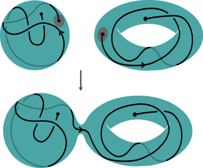
Figure 3: Product of a knotoid diagram in sphere and a knotoid diagram in torus.

Remark 2.1.1.

The notion of knotoids can be extended by allowing the domain of immersion to include a finite number of circles in addition to the unit interval. The resulting diagrams are called multi-knotoid diagrams. Multi-knotoids are then equivalence classes of multi-knotoid diagrams considered up to Reidemeister moves and isotopy of $\Sigma$.

By adding the point at infinity to $\mathbb{R}^{2}$, every planar knotoid diagram can be mapped to a spherical knotoid diagram. However, there exist non-trivial planar knotoid diagrams which map to spherical knotoid diagrams that are equivalent to trivial knotoid diagrams in $S^{2}$. An example is shown in Figure 1b. The reason behind this is as follows. Think of $S^{2}$ as $\mathbb{R}^{2}\cup\infty$. Then it is clear that the spherical isotopy not only includes planar isotopy but also lets an arc of a diagram pass through the point at infinity, which transforms the non-trivial planar knotoid diagram in Figure 1b into a trivial one in $S^{2}$. This implies that planar knotoids are not in a one-to-one correspondence with spherical knotoids.

2.2 Classical Knots and Knotoids

One can tie up the endpoints of a knotoid diagram in $S^{2}$ or $\mathbb{R}^{2}$ to obtain a (classical) knot diagram with underpass or overpass closures. The underpass (overpass) closure of a knotoid diagram is obtained by connecting the endpoints of a knotoid diagram by an arc which goes under (over) every other arc it meets along the way. The resulting diagram is clearly a knot diagram which represents a knot in $S^{3}$ (a classical knot). The underpass and overpass closures may represent inequivalent knots. We exemplify this in Figure 4 where the underpass closure of a knotoid diagram represents the trefoil knot, while the overpass closure represents the unknot. To have a well-defined closure on knotoid diagrams, we fix the closure type we want to use to obtain knots from knotoids. We have the following theorem by fixing the closure as the underpass closure.

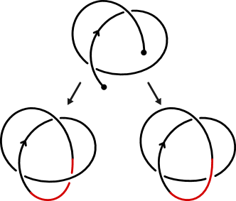
Figure 4: The underpass (on the left) and overpass (on the right) closures of a knotoid diagram.

Theorem 2.2.1.

[16] The underpass closures of two knotoid diagrams in $S^{2}$ represent the same knot if and only if they are related to each other by finitely many Reidemeister moves and forbidden $\Omega_{-}$ moves.

By Theorem 2.2.1 we can consider the collection of spherical knotoid diagrams representing a classical knot via the underpass closure as knotoid representations of the knot. In [16] Turaev suggests to utilize knotoids in computing knot invariants, as they provide simpler representations of classical knots possibly with fewer crossings than knot diagrams.

Every oriented knot diagram in $S^{2}$ can be turned into a knotoid diagram by cutting an arc that does not contain any of the crossings of the diagram. The endpoints of the resulting knotoid diagram are clearly in the same region. Such diagrams are called knot-type knotoid diagrams. A knot-type knotoid carries the same topological information as the knot obtained by its underpass closure. That is, there is a one-to-one correspondence between knot-type knotoids in $S^{2}$ and classical knots.

The spherical knotoid theory can be viewed as an extension of the classical knot theory with the existence of proper knotoids. A proper knotoid is a knotoid without any representative knotoid diagrams in its equivalence class that has its endpoints in the same region. Thus, a proper knotoid is not induced from a classical knot by the cutting operation explained above.

2.3 Geometric Interpretations of Spherical and Planar Knotoids

In [16] Turaev shows that spherical knotoids can be interpreted as theta-curves in $S^{3}=\mathbb{R}^{3}\cup\infty$.

Definition 2.3.1.

A theta-curve is a directed graph embedded in $S^{3}$ consisting of two vertices, labeled $v_{0},v_{1}$ and three edges connecting these two vertices labeled $e_{+},e_{0},e_{-}$, considered up to label-preserving isotopies of $S^{3}$. The edges of a theta-curve is directed from $v_{0}$ to $v_{1}$. A theta-curve is called simple if the edges $e_{+}$ and $e_{-}$ bound a unique disk in $S^{3}$.

Definition 2.3.2.

Let $\theta^{\prime}$ and $\theta^{\prime\prime}$ be two theta-curves. Let $B^{\prime}$ and $B^{\prime\prime}$ be regular neighborhoods of vertices $v_{1}^{\prime}$ of $\theta^{\prime}$ and $v_{0}^{\prime\prime}$ of $\theta^{\prime\prime}$, respectively. The vertex multiplication of $\theta^{\prime}$ and $\theta^{\prime\prime}$, denoted by $\theta^{\prime}\theta^{\prime\prime}$, is a theta-curve resulting from the gluing of $S^{3}-\text{Int}(B^{\prime})$ and $S^{3}-\text{Int}(B^{\prime\prime})$ along an orientation-reversing homeomorphism $\varphi:\partial(B^{\prime})\rightarrow\partial(B^{\prime\prime})$ such that the intersection point $e_{i}^{\prime}\cap\partial(B^{\prime})$ gets mapped to the intersection point $e_{i}^{\prime\prime}\cap\partial(B^{\prime\prime})$ for $i=+,0,-$. See Figure 5 for an illustration of vertex multiplication. The vertex multiplication on theta-curves induces a semigroup structure on theta-curves.

\begin{overpic}[width=241.84842pt]{untitled.png} \put(20.0,33.0){$e_{+}^{\prime}$} \put(15.0,22.0){$e_{0}^{\prime}$} \put(20.0,0.0){$e_{-}^{\prime}$} \put(77.0,33.0){$e_{+}^{\prime\prime}$} \put(70.0,11.0){$e_{0}^{\prime\prime}$} \put(77.0,0.0){$e_{-}^{\prime\prime}$} \put(53.0,17.0){$v_{0}^{\prime\prime}$} \put(100.0,17.0){$v_{1}^{\prime\prime}$} \put(-2.5,17.0){$v_{0}^{\prime}$} \put(45.0,17.0){$v_{1}^{\prime}$} \end{overpic}

(a) Two theta-curve examples, $\theta^{\prime}$ and $\theta^{\prime\prime}$.

\begin{overpic}[width=241.84842pt]{theta2.png} \put(42.0,10.0){$B^{\prime}$} \put(52.5,10.0){$B^{\prime\prime}$} \end{overpic}

(b) Two regular neighbourhoods $B^{\prime}$ and $B^{\prime\prime}$ around the vertices $v_{1}^{\prime}$ and $v_{0}^{\prime\prime}$.

\begin{overpic}[width=241.84842pt]{theta3.png} \put(-3.0,15.0){$v_{0}$} \put(100.0,13.0){$v_{1}$} \end{overpic}

(c) $\theta=\theta^{\prime}\theta^{\prime\prime}.$

Figure 5: The vertex multiplication of theta-curves.

One can construct a theta-curve $\theta$ from a knotoid diagram $K$ in $\mathbb{R}^{2}$. Consider $\mathbb{R}^{2}$ as $\mathbb{R}^{2}\times\{0\}\subset\mathbb{R}^{3}$, and the tail and head of $K$ as the vertices $v_{0}$ and $v_{1}$ of $\theta$, respectively. The edge $e_{0}$ of $\theta$ is formed by pushing the overpassing strands of $K$ in $\mathbb{R}^{2}\times\mathbb{R}^{+}$. The edges $e_{+}$ and $e_{-}$ of $\theta$ are formed by pushing an embedded arc in $\mathbb{R}^{2}\times\{0\}$ connecting the vertices $v_{0}$ and $v_{1}$ to $\mathbb{R}^{2}\times\mathbb{R}^{+}$ and $\mathbb{R}^{2}\times\mathbb{R}^{-}$, respectively. It is clear that $e_{+}\cup e_{0}\cup e_{-}$ is a simple theta-curve in $S^{3}$.

This construction induces a bijective map between spherical knotoids and simple theta-curves in $S^{3}$. In fact, we have the following theorem.

Theorem 2.3.1.

[16] There is an isomorphism between the semigroup of knotoids in $S^{2}$ and the semigroup of simple theta-curves in $S^{3}$.

In [8] the first author and Kauffman give a three-dimensional interpretation for planar knotoids as follows. Let $K$ be a knotoid in $\mathbb{R}^{2}$. Identify $\mathbb{R}^{3}$ with $\mathbb{R}^{2}\times\mathbb{R}$ so that $K$ can be considered lying in $\mathbb{R}^{2}\times\{0\}$, and can be embedded in $\mathbb{R}^{3}$ by pushing the overpassing strands to $\mathbb{R}^{2}\times\mathbb{R^{+}}$ and underpassing strands to $\mathbb{R}^{2}\times\mathbb{R^{-}}$, while the endpoints of $K$ are kept attached on two distinct parallel lines that are orthogonal to the plane where $K$ lies. In this way, an open, oriented smooth curve embedded in $\mathbb{R}^{3}$ is obtained.

Conversely, any open, oriented curve in $\mathbb{R}^{3}$ that is generic to the xy-plane can be projected onto the plane to obtain a knotoid diagram. The one-to-one correspondence between knotoids in $\mathbb{R}^{2}$, and open, oriented smooth curves in $\mathbb{R}^{3}$ is obtained by defining line isotopy for space curves.

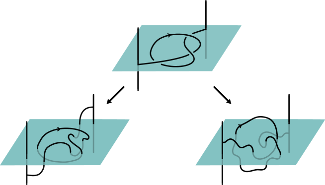
Figure 6: Two different embeddings of a knotoid diagram in $\mathbb{R}^{3}$.

Definition 2.3.3.

Let $K_{1}$ and $K_{2}$ be two smooth, open and oriented curves embedded in $\mathbb{R}^{3}$ with the endpoints corresponding to points on the lines $t_{1}\times\mathbb{R}$, $h_{1}\times\mathbb{R}$ and $t_{2}\times\mathbb{R}$, $h_{2}\times\mathbb{R}$. $K_{1}$ and $K_{2}$ are said to be line isotopic if there is a smooth ambient isotopy of $\mathbb{R}^{3}$, taking one curve to the other curve in the complement of the lines, taking the tail and head of $K_{1}$ to the tail and head of $K_{2}$, and taking lines to lines; $t_{1}\times\mathbb{R}$ to $t_{2}\times\mathbb{R}$ and $h_{1}\times\mathbb{R}$ to $h_{2}\times\mathbb{R}$.

Theorem 2.3.2.

[8] Two open oriented curves embedded in $\mathbb{R}^{3}$, which are both generic to xy-plane, are line isotopic (with respect to the lines determined by the endpoints of the curves) if and only if the projections of the curves to $\mathbb{R}^{2}\times\{0\}$ are equivalent knotoid diagrams.

The approach used in the geometric interpretation of planar knotoids given above has found key applications in studying protein folding. See [7][4][5].

2.4 Virtual Knots and Knotoids

We begin by reviewing the theory of virtual knots that was introduced by Louis H. Kauffman in 1996.

Definition 2.4.1.

A virtual knot/link is a knot/link in a thickened surface $\Sigma\times I$, where $I$ denotes the unit interval $[0,1]$ (see Figure 7a for an example of a virtual knot in thickened torus).

Definition 2.4.2.

Let $V$ be a virtual knot/link in a thickened surface $\Sigma\times I$. Let $B_{1},B_{2}$ be two disjoint open disks in $\Sigma$ such that $B_{1}\times I$ and $B_{2}\times I$ do not intersect $V$. The stabilization operation consists of removing the two open annuli $B_{1}\times I$ and $B_{2}\times I$ from $\Sigma\times I$, and attaching a thickened handle $S^{1}\times I\times I$ by gluing the annuli $S^{1}\times\{0\}\times I$ and $S^{1}\times\{1\}\times I$ to the boundaries of removed annuli in $\Sigma\times I$.

Definition 2.4.3.

The destabilization is defined as the inverse operation of stabilization. Let $C$ be a simple closed curve in $\Sigma$ such that $C\times I$ is disjoint from $V$ and does not bound a ball in $\Sigma\times I-V$. The destabilization operation consists of cutting $\Sigma\times I$ along the vertical annulus $C\times I$, and capping the two resulting annuli with thickened disks $D^{2}\times I$. The annulus $C\times I$ is called a destabilization annulus. Figure 8 illustrates a destabilization annulus for the given virtual knot.

Definition 2.4.4.

Two virtual knots/links, not necessarily lying in the same thickened surface, are considered to be stably equivalent if they can be obtained from one another by isotopy of the thickened surfaces, homeomorphisms of the surfaces and stabilization/destabilization operations.

\begin{overpic}[width=303.53267pt]{virtualknots.pdf} \put(20.0,22.0){\footnotesize(a)} \put(73.0,24.0){\footnotesize(b)} \put(73.0,-4.0){\footnotesize(c)} \end{overpic}

Figure 7: A virtual knot and its projections.

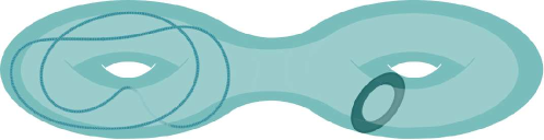
Figure 8: Example of a destabilization annulus.

Definition 2.4.5.

A virtual knot in a thickened surface is called irreducible if the thickened surface has no (thickened) handles that are disjoint from the virtual knot, that is, if it admits no destabilizations.

In [14], G. Kuperberg proves the following theorem for virtual knots utilizing geometric arguments from three-dimensional topology that we also use to prove our main theorem in Section 3.2.

Theorem 2.4.1.

[14] Every virtual knot in thickened surfaces has a unique irreducible virtual knot representation.

A classical knot can be considered as a virtual knot that has an irreducible representation in $S^{2}\times I$. From Theorem 2.4.1 it follows that classical knots have unique representations. That is, if two classical knots are stably equivalent to each other then they can be turned to each other by only a series of classical Reidemeister moves. With this observation, it can be deduced that virtual knot theory properly extends the theory of classical knots.

Virtual knots/links can also be studied through their diagrams on surfaces up to Reidemeister moves, homeomorphism of surfaces and handle stabilization/destabilization of surfaces (see Figure 7b for a diagram of the given virtual knot on torus) or as purely combinatorially through virtual knot diagrams in the plane (see Figure 7c).

Definition 2.4.6.

A virtual knot/link diagram in the plane is a planar representation of a virtual knot that is an immersed closed curve whose each self-intersection is declared as either a classical crossing or a virtual crossing. A virtual crossing is indicated by a circle around a transversal intersection that provides no under or over information unlike a classical crossing.

Note that a classical crossing of a virtual knot diagram represents the weaving type of the virtual knot in the thickened surface on which it lies, while a virtual crossing can be considered as an artifact of representing the virtual knot in the plane.

The equivalence relation on the virtual knot diagrams in the plane is induced by the classical Reidemeister moves shown in Figure 9(a), plus the moves containing virtual crossings shown in Figures 9(b) and 9(c).

\begin{overpic}[width=113.81102pt]{classicalreidemoves2.pdf} \end{overpic}

(a) Classical Reidemeister moves.

\begin{overpic}[width=113.81102pt]{virtualreidemoves.pdf} \end{overpic}

(b) Virtual Reidemeister moves.

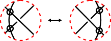
(c) Mixed virtual move.

Figure 9: Moves for virtual knot diagrams in the plane.

Definition 2.4.7.

A virtual knot is an equivalence class of equivalent virtual knot diagrams in the plane.

Remark 2.4.1.

A classification table of virtual knots with up to four crossings can be found in [6]. Following this work, a table of virtual links with two components and up to four crossings is given in [2].

In [16] it was mentioned that knotoids can be studied in virtual setting. This can be done by obtaining a virtual knot diagram from a knotoid diagram in $\mathbb{R}^{2}$ or $S^{2}$ using the virtual closure or considering a knotoid diagram with virtual crossings, as we explain below.

Definition 2.4.8.

The virtual closure of a knotoid diagram $K$ is connecting the tail and head of $K$ by an arc so that each of its intersections with $K$ is declared as a virtual crossing.

It was shown in [8] that the virtual closure induces a well-defined map from the set of spherical knotoids into the set of virtual knots. Being a well-defined map, any virtual knot invariant can be considered as an invariant of spherical knotoids through the virtual closure. See [8] for more details.

Virtual knotoid diagrams were introduced in [8] as a generalization of knotoids in $S^{2}$ as follows.

Definition 2.4.9.

A virtual knotoid diagram is a knotoid diagram in $S^{2}$ with finitely many virtual crossings. Some examples of virtual knotoid diagrams are given in Figure 10.

Figure 10: Virtual knotoid diagrams.

Definition 2.4.10.

Two virtual knotoid diagrams are considered to be equivalent if they can be obtained from each other by a series of moves given also for virtual knot diagrams (classical and virtual Reidemeister moves, and the mixed virtual move) in Figure 9, plus the virtual endpoint move given in Figure 11 that moves the arc adjacent to an endpoint through a transversal arc by deleting/adding a virtual crossing. Notice that forbidden moves of knotoid diagrams are also forbidden for virtual knotoid diagrams.

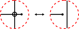
Figure 11: Virtual endpoint move.

Definition 2.4.11.

A virtual knotoid is an equivalence class of virtual knotoid diagrams in $S^{2}$.

It was shown in [8] that virtual knotoids in $S^{2}$ are in a one-to-one correspondence with the equivalence classes of knotoid diagrams in surfaces. This correspondence is provided by abstract knotoid diagrams.

An abstract knotoid diagram is a closed, connected, and orientable ribbon surface with boundary that is associated with a knotoid diagram $K$ as follows. To each classical crossing and each endpoint of $K$, we attach 2-disks and then connect these disks by ribbons that contain semi-arcs of $K$. Whenever these ribbons meet at a virtual crossing we want them to pass over one another. See Figure 12 for an illustration.

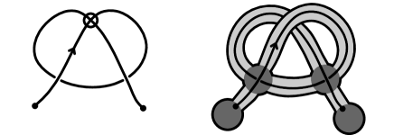
Figure 12: An abstract knotoid diagram obtained from a given virtual knotoid diagram.

Conversely, one can obtain a unique virtual knotoid diagram from an abstract knotoid diagram as follows. Firstly, we embed an abstract knotoid diagram in $S^{3}$ in such a way that the disks surrounding the classical crossings and the endpoints are mapped on a sphere $S^{2}$ in $S^{3}$. Then we project this embedding to $S^{2}$ in a way such that the projections of the arcs that lie in ribbon bands either do not intersect or intersect transversally under this projection. We mark the transversal intersections in the projection as virtual crossings. The resulting object is a virtual knotoid diagram in $S^{2}$.

Abstract knotoid diagrams are considered up to an equivalence relation induced by generalized abstract moves depicted in Figure 13. An equivalence class of abstract knotoid diagrams is called an abstract knotoid.

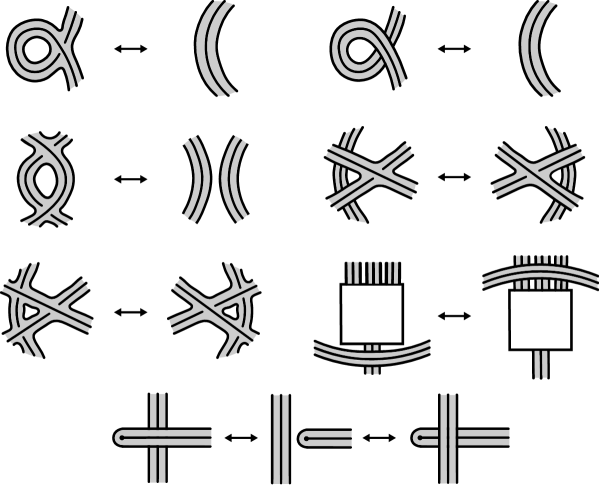
Figure 13: Abstract moves defined on abstract knotoid diagrams.

The two operations given above induce mappings between virtual knotoids in $S^{2}$ and abstract knotoids, which are inverses of each other. Thus, we have the following theorem.

Theorem 2.4.2.

[8] There is a one-to-one correspondence between virtual knotoids in $S^{2}$ and abstract knotoids.

We now consider knotoid diagrams in surfaces. By extending the equivalence relation defined for knots in surfaces it is possible to define an equivalence of two knotoid diagrams in surfaces with different genera.

Definition 2.4.12.

Let $K_{1}$ and $K_{2}$ be two knotoid diagrams in surfaces $\Sigma_{1}$ and $\Sigma_{2}$ with possibly different genera. Then $K_{1}$ and $K_{2}$ are called stably equivalent if they can be obtained from each other by finitely many Reidemeister moves in the surfaces, isotopy of the surfaces and handle stabilization/destabilization in the complement of the diagrams. The resulting equivalence classes are called stable equivalence classes of knotoids.

Let $D$ be an abstract knotoid diagram. Filling the boundaries of $D$ with 2-disks results in a closed connected orientable surface containing the knotoid diagram $D$. Conversely, given a knotoid diagram $K$ in the surface $\Sigma$, the tubular neighborhood of $K$ is an abstract knotoid diagram. These two operations induce mappings between abstract knotoids and stable equivalence classes of knotoid diagrams. In fact, we have the following statement.

Theorem 2.4.3.

[8] There is a one-to-one correspondence between abstract knotoids and stable equivalence classes of knotoid diagrams in surfaces.

Theorem 2.4.2 combined with Theorem 2.4.3 gives the following main theorem.

Theorem 2.4.4.

[8] There is a one-to-one correspondence between virtual knotoids and stable equivalence classes of knotoid diagrams in higher genus surfaces.

3 An Interpretation of Virtual Knotoids in Thickened Surfaces

In this section, we introduce virtual arcs embedded in thickened surfaces. Through the projections of these arcs, we obtain knotoid diagrams in surfaces, and we establish a correspondence between the equivalence classes of virtual arcs and the stable equivalence classes of knotoid diagrams in surfaces.

3.1 Virtual Arcs

We adopt the three-dimensional interpretation of planar knotoids given in [8] to define virtual arcs. Note that virtual arcs can be considered as H-curves studied in [3].

Definition 3.1.1.

Let $\Sigma$ be a closed, connected, and oriented surface and $t$, $h$ be two distinct points in $\Sigma$. A virtual arc $\boldsymbol{\upsilon}$ is an embedding of the unit interval in the thickened surface $\Sigma\times I$ such that $\text{Im}(\boldsymbol{\upsilon})\cap(t\times I)=\boldsymbol{\upsilon}(0)$ and $\text{Im}(\boldsymbol{\upsilon})\cap(h\times I)=\boldsymbol{\upsilon}(1)$. That is, a virtual arc is a simple curve in the thickened surface $\Sigma\times I$ that starts at a point on $t\times I$ and ends at a point on $h\times I$ (see Figure 14 for an example of a virtual arc in thickened torus). The points $\boldsymbol{\upsilon}(0)$ and $\boldsymbol{\upsilon}(1)$ that lie on $t\times I$ and $h\times I$, respectively, are the endpoints of the arc. The endpoint $\boldsymbol{\upsilon}(0)$ is called the tail and the endpoint $\boldsymbol{\upsilon}(1)$ is called the head of $\boldsymbol{\upsilon}$. We call the line segments $t\times I$ and $h\times I$ the rails of the virtual arc $\boldsymbol{\upsilon}$ following the terminology used in [13] in the definition of rail arcs in $\mathbb{R}^{3}$.

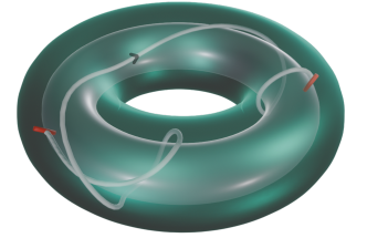
Figure 14: A virtual arc in a thickened torus.

Definition 3.1.2.

Let $\boldsymbol{\upsilon}$ be a virtual arc in the thickened surface $\Sigma\times I$ with rails $t\times I$ and $h\times I$. $\boldsymbol{\upsilon}$ is called trivial if it embeds in $\sigma\times I$ where $\sigma$ is a virtual arc in the surface $\Sigma\times\{0\}$ with endpoints $t\times\{0\}$ and $h\times\{0\}$.

We now introduce an analog of the isotopy given in Definition 2.3.3 for thickened surfaces. Then we describe the handle stabilization/destabilization operations for a virtual arc in a thickened surface.

Definition 3.1.3.

Let $\boldsymbol{\upsilon}_{i}$ be a virtual arc in $\Sigma\times I$ with its rails $t_{i}\times I$ and $h_{i}\times I$, for $i=1,2$. $\boldsymbol{\upsilon}_{1}$ and $\boldsymbol{\upsilon}_{2}$ are said to be arc isotopic if there is a smooth ambient isotopy of $\Sigma\times I$, taking one arc to the other arc in the complement of the rails $t_{i}\times I$ and $h_{i}\times I$, taking endpoints to endpoints; $(t_{1},x_{1})$ to $(t_{2},x_{2})$ and $(h_{1},y_{1})$ to $(h_{2},y_{2})$, and taking rails to rails; $t_{1}\times I$ to $t_{2}\times I$ and $h_{1}\times I$ to $h_{2}\times I$.

In our interpretation, we need to take extra care of the rails $t\times I$ and $h\times I$ of the virtual arc $\boldsymbol{\upsilon}\subset\Sigma\times I$. In particular, whenever we perform an operation, aside from the ambient isotopy, on the ambient thickened surface, we need to make sure that we remove not only the virtual arc itself but also its rails from the space. In other words, instead of $(\Sigma\times I)\;-\;\boldsymbol{\upsilon}$, the operation is performed in $(\Sigma\times I)\;-\;(\boldsymbol{\upsilon}\cup(\{t,h\}\times I))$.

Definition 3.1.4.

Consider a virtual arc $\boldsymbol{\upsilon}$ in a thickened surface $\Sigma\times I$ with its rails $t\times I$ and $h\times I$. Let $\boldsymbol{|\upsilon|}$ denote the union of $\boldsymbol{\upsilon}$ and its rails $t\times I$ and $h\times I$. Let $B_{1},B_{2}$ be two disjoint open disks in $\Sigma$ such that $B_{1}\times I$ and $B_{2}\times I$ does not intersect $\boldsymbol{|\upsilon|}$. The stabilization operation consists of removing the two open cylinders $B_{1}\times I$ and $B_{2}\times I$ from $\Sigma\times I$, and attaching a thickened handle $S^{1}\times I\times I$ by gluing annuli $S^{1}\times\{0\}\times I$ and $S^{1}\times\{1\}\times I$ to the boundaries of removed open cylinders in $\Sigma\times I$. Let $C$ be a simple closed curve in $\Sigma$ such that $C\times I$ is disjoint from $\boldsymbol{|\upsilon|}$ and it does not bound a ball in $(\Sigma\times I)-\boldsymbol{|\upsilon|}$. The destabilization operation consists of cutting $\Sigma\times I$ along the vertical annulus $C\times I$, and capping the two resulting annuli with thickened disks $D^{2}\times I$.

Remark 3.1.1.

We consider destabilization annuli up to isotopy in $\Sigma\times I$, following the same notion as in [14]. We let any isotopic image of the annulus $C\times I$ mentioned in Definition 3.1.4 to be a destabilization annulus.

Definition 3.1.5.

The arc isotopies of $\;\Sigma\times I$, homeomorphisms of $\Sigma$ and stabilizations/destabilizations of $\Sigma\times I$ induce an equivalence relation in the set of virtual arcs in thickened surfaces, and it is called virtual arc equivalence.

From now on, we consider the equivalence classes of virtual arcs with respect to the virtual arc equivalence. We use the notation $(\boldsymbol{\upsilon},\Sigma\times I)$ for a virtual arc $\boldsymbol{\upsilon}$ in the thickened surface $\Sigma\times I$. The projection of $\boldsymbol{\upsilon}$ on the surface $\Sigma$ by the map

$$p:\Sigma\times I \rightarrow\Sigma$$

$$(x,t) \mapsto x$$

equiped with under or over information at the crossings gives a diagram of $\boldsymbol{\upsilon}$. The resulting diagram is a knotoid diagram in the surface $\Sigma$.

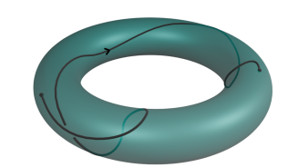
Figure 15: The diagram of the virtual arc given in Figure 14.

Theorem 3.1.1.

Two virtual arcs $(\boldsymbol{\upsilon},\Sigma\times I)$ and $(\boldsymbol{\upsilon}^{\prime},\Sigma^{\prime}\times I)$ are virtually equivalent if and only if their diagrams in $\Sigma$ and $\Sigma^{\prime}$ are stably equivalent.

To prove Theorem 3.1.1, we view virtual arcs as piecewise-linear arcs. That is, a virtual arc is represented as the union of finitely many edges $[p_{1}p_{2}],\;[p_{2}p_{3}],\;...,\;[p_{n-1}p_{n}]$, such that $p_{1}$ and $p_{n}$ correspond to the tail and head of the virtual arc, respectively. Each pair of edges of a virtual arc can only intersect at a point $p_{i}$, where $i\in\{2,3,...,n-1\}$.

Definition 3.1.6.

Let $[p_{i}p_{i+1}]$ be an edge of a piecewise-linear representation of a virtual arc $\boldsymbol{\upsilon}$ in $\Sigma\times I$, and let $p_{0}$ be a point in the complement of $\boldsymbol{|\upsilon|}$ such that $[p_{i}p_{0}],[p_{0}p_{i+1}]\subset\Sigma\times I$ and the triangle $\overset{\triangle}{p_{i}p_{0}p_{i+1}}$ bounds a disk in $(\Sigma\times I)-\boldsymbol{|\upsilon|}$. We define the triangle move in the thickened surface $\Sigma\times I$ as the transformation of $[p_{i}p_{i+1}]$ into two edges $[p_{i}p_{0}]$ and $[p_{0}p_{i+1}]$. The inverse triangle move is the transformation of two consecutive edges into one edge that satisfies the condition that the triangular region formed by these three edges bounds a disk in $\Sigma\times I-\boldsymbol{|\upsilon|}$. These two moves are denoted by $\Delta^{+1}$ and $\Delta^{-1}$, respectively.

The equivalence of virtual arcs can be expressed as the equivalence of piecewise-linear representations of virtual arcs. Two representations are equivalent if one can be deformed into the other by a finite sequence of $\Delta^{\pm 1}$ moves. Equipped with these, we now give the proof of Theorem 3.1.1.

Proof.

First, note that we can think of the possible steps of obtaining $(\boldsymbol{\upsilon}^{\prime},\Sigma^{\prime}\times I)$ from $(\boldsymbol{\upsilon},\Sigma\times I)$ in two parts; handle stabilizations/destabilizations of the thickened surface and arc isotopies. It is easy to see that the handle stabilizations/destabilizations of a thickened surface $\Sigma\times I$ are captured by handle stabilizations/destabilizations of the underlying surface $\Sigma$, and vice versa. It is also easy to see that moves on a knotoid diagram are captured by the arc isotopies in the thickened surface. To prove that the arc isotopies are captured by the moves in the diagrams, we show that all possible shadows of the triangle moves are generated by the Reidemeister moves in $\Sigma$. To do so, we use induction on the number of strands, denoted by $n$, in the shadow of a triangle move. Figure 16 shows that the isotopies of $\Sigma$ and Reidemeister moves are, respectively, enough for cases $n=0,1,2$. For $n\geq 3$, we apply subdivision on the edges of the triangle and express the triangle move as a finite sequence of triangle moves where $n\leq 2$. ∎

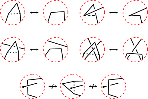
Figure 16: Shadows of triangle moves in surface $\Sigma$.

3.2 Unifying the Interpretations

As explained in Section 2.3, virtual knotoid theory has an interpretation as stable equivalence classes of knotoid diagrams in surfaces. An interpretation of the latter theory is given in Section 3.1 as virtual arcs in thickened surfaces. Here we combine these two interpretations to give a geometric interpretation of virtual knotoids.

Theorem 3.2.1.

The virtual arc theory in thickened surfaces is equivalent to the virtual knotoid theory given diagrammatically in $S^{2}$.

Proof.

Theorem 2.4.4 states that the equivalence classes of the virtual knotoid diagrams in $S^{2}$ are in one-to-one correspondence with the stable equivalence classes of knotoid diagrams in surfaces. Theorem 3.1.1 states that the equivalence classes of virtual arcs in thickened surfaces are in one-to-one correspondence with the stable equivalence classes of knotoid diagrams in the underlying surfaces. By combining these two theorems, we obtain a correspondence between virtual knotoids in $S^{2}$ and the equivalence classes of virtual arcs in the thickened surfaces. ∎

Theorem 3.2.1 allows us to refer to the equivalence classes of virtual arcs in thickened surfaces as virtual knotoids throughout the rest of the paper.

Definition 3.2.1.

Let $(\boldsymbol{\upsilon},\Sigma\times I)$ be a virtual knotoid. If the complement of $\boldsymbol{|\upsilon|}$ in $\Sigma\times I$ does not have empty thickened handles, then $(\boldsymbol{\upsilon},\Sigma\times I)$ is called an irreducible virtual knotoid.

Remark 3.2.1.

Note that by fixing the thickened surface as $S^{2}\times I$, and restricting the equivalence relation to be up to only arc isotopies of $S^{2}\times I$ in our interpretation, we obtain a geometric interpretation of classical knotoids in $S^{2}$. Thus, we refer this setting as classical knotoid theory. A classical knotoid may be also regarded as a virtual knotoid when it is considered up to virtual equivalence. In this setting a classical knotoid is a virtual knotoid with at least one irreducible representation in $S^{2}\times I$.

We are now ready to prove our main theorem, namely Theorem 3.2.2. We prove this theorem by extending the arguments utilized in [14] to virtual knotoids. Note that our main focus in this paper is to give a geometric interpretation of virtual knotoids but the arguments can be extended directly to multi-component case.

Theorem 3.2.2.

Every virtual knotoid is uniquely represented by an irreducible virtual knotoid.

Proof.

We prove the statement by contradiction. Assume that there exist virtual knotoids that admit multiple irreducible representations. Suppose that the genus of thickened surfaces of such virtual knotoids is at least $g$, for some $g\in\mathbb{N}$. Consider the collection $\mathcal{M}=\{(\boldsymbol{\upsilon},\Sigma\times I)\}$ of such virtual knotoids where $\Sigma$ has genus $g$. It is clear that depending on the annulus we destabilize $(\boldsymbol{\upsilon},\Sigma\times I)\in\mathcal{M}$ along, we may end up with multiple destabilizations that are not isotopic and that any destabilization of $(\boldsymbol{\upsilon},\Sigma\times I)$ has genus $g-1$. Then, by assumption, each of these destabilizations admits a unique irreducible representation.

Let $A_{1}$ and $A_{2}$ be two disjoint annuli along which we can destabilize $(\boldsymbol{\upsilon},\Sigma\times I)$. Let $(\boldsymbol{\upsilon},\Sigma_{A_{1}}\times I)$ and $(\boldsymbol{\upsilon},\Sigma_{A_{2}}\times I)$ be destabilizations of $(\boldsymbol{\upsilon},\Sigma\times I)$ along $A_{1}$ and $A_{2}$. If $A_{1}$ and $A_{2}$ are parallel in $\Sigma\times I$, then the destabilizations along these annuli are isotopic. If they are not parallel, we destabilize $(\boldsymbol{\upsilon},\Sigma_{A_{1}}\times I)$ and $(\boldsymbol{\upsilon},\Sigma_{A_{2}}\times I)$ along $A_{2}$ and $A_{1}$, respectively, to obtain a common destabilization $(\boldsymbol{\upsilon},\Sigma_{c}\times I)$. Notice that $(\boldsymbol{\upsilon},\Sigma_{c}\times I)$ has a unique irreducible representation which is also the unique irreducible representation of both $(\boldsymbol{\upsilon},\Sigma_{A_{1}}\times I)$ and $(\boldsymbol{\upsilon},\Sigma_{A_{2}}\times I)$ since each of them has genus less than $g$. We illustrate this in Figure 17. This sets a contradiction with the assumption that $(\boldsymbol{\upsilon},\Sigma\times I)$ has multiple inequivalent irreducible representations.

Figure 17: A diagram of destabilizations $(\boldsymbol{\upsilon},\Sigma\times I)$ along annuli $A_{1}$ and $A_{2}$. An arrow with an indicator $A_{i}$ means that the thickened surface at the head of the arrow is obtained by destabilization of the thickened surface at the tail of the arrow along $A_{i}$.

Now we consider non-disjoint pairs of destabilization annuli of $(\boldsymbol{\upsilon},\Sigma\times I)$ in general position such that the destabilizations of $(\boldsymbol{\upsilon},\Sigma\times I)$ along these annuli have inequivalent unique irreducible representations. Among such pairs of annuli, consider $A_{1}$ and $A_{2}$ which intersect at the least number of curves. Let the number of curves in $A_{1}\cap A_{2}$ be $k$. Note that this assumption implies that any two destabilizations of $(\boldsymbol{\upsilon},\Sigma\times I)$ along a pair of annuli that intersect at less than $k$ curves have equivalent unique irreducible representations.

Let $C$ be a curve in $A_{1}\cap A_{2}$. Then, there are four possible cases. If $C$ is open, either it is vertical so that its endpoints are in different components of $\partial A_{i=1,2}$, see Figure 18(a), or it bounds a disk in $A_{i}$ with a part of $\partial A_{i}$. If $C$ is closed, either it is horizontal so that it is parallel to the boundaries of $A_{1}$ and $A_{2}$, see Figure 18(b), or it bounds a disk in $A_{i}$.

\begin{overpic}[width=184.9429pt]{case1} \end{overpic}

(a) Vertical intersection open curves.

\begin{overpic}[width=156.49014pt]{case2.pdf} \end{overpic}

(b) A horizontal intersection closed curve.

Figure 18: Examples of intersection curves.

We first consider the cases where $C$ is a non-vertical open curve or a non-horizontal closed curve in $A_{i}$. Then $C$ is either the boundary or part of the boundary of a disk, say $D$, in $A_{i}$. We compress $A_{3-i}$ along $D$ (see Figure 19 for an illustration of such compression). This operation splits $A_{3-i}$ into two disjoint parts: a destabilization annulus $A_{3-i}^{{}^{\prime}}$ and a part that bounds a ball in the complement of $\boldsymbol{|\upsilon|}$. The intersections $A_{i}\cap A_{3-i}^{{}^{\prime}}$ and $A_{3-i}\cap A_{3-i}^{{}^{\prime}}$ both consist of fewer than $k$ curves. Thus, the destabilizations along $A_{i}$, $A_{3-i}$, and $A_{3-i}^{{}^{\prime}}$ have equivalent unique irreducible representations. This sets a contradiction.

\begin{overpic}[width=160.43727pt]{compression.pdf} \put(13.0,51.0){D} \put(3.0,-3.0){$A_{3-i}$} \put(32.0,-3.0){$A_{i}$} \put(60.0,-3.0){$A_{3-i}^{\prime}$} \put(92.0,-3.0){$A_{i}$} \end{overpic}

Figure 19: An illustration of the compression.

Now suppose that $A_{1}\cap A_{2}$ consists of $k$ vertical open curves. Consider $A_{1}\cup A_{2}$. Let $U$ be a regular neighborhood of $A_{1}\cup A_{2}$ that does not intersect $\boldsymbol{|\upsilon|}$. Then $\partial U=U_{1}\cup U_{2}\cup...\cup U_{n}$, where $U_{j}$ is a vertical annulus in $\Sigma\times I$ for $j=1,...,n$ (see Figure 20 for an example case where $n=4$). Clearly, $A_{i}\cap U_{j}=\emptyset$ for all $j=1,...n$, and $\Sigma\times I\;-\;\partial U$ consists of a number of disjoint components. Notice that the virtual knotoid $\boldsymbol{\upsilon}$ lies in exactly one of these components. Now we examine the possible cases for $U_{j=1,...,n}$.

• If none of $U_{j=1,...,n}$ is a destabilization annulus, that is, each of them bounds a ball in $\Sigma\times I$, then one of them separates $A_{1}\cup A_{2}$ from $\boldsymbol{|\upsilon|}$. In this case, neither $A_{1}$ nor $A_{2}$ can be destabilization annuli as they lie in the ball bounded by one of $U_{j}$. Thus, we have a contradiction.

• Suppose now that for some $i\in\{1,...n\}$, $U_{i}$ is a destabilization annulus. Since it does not intersect with $A_{1}$ (or $A_{2}$), destabilization along $U_{i}$ induces an equivalent unique irreducible representation with destabilization along $A_{1}$ (or $A_{2}$) by assumption. Thus, the destabilizations of $(\boldsymbol{\upsilon},\Sigma\times I)$ along $A_{1}$ and $A_{2}$ have equivalent unique irreducible representations, which is a contradiction.

\begin{overpic}[width=99.73074pt]{lastcase.pdf} \put(8.0,25.0){$U_{1}$} \put(14.0,75.0){$U_{2}$} \put(76.0,24.0){$U_{3}$} \put(83.0,72.0){$U_{4}$} \end{overpic}

Figure 20: The boundary of a regular neighborhood of $A_{1}\cup A_{2}$, where $A_{i=1,2}$ is a destabilization annulus.

Next, suppose that $A_{1}\cap A_{2}$ consists of closed horizontal curves $C_{1},...,C_{k}$, that is, $C_{j=1,...,k}$ does not bound a disk in $A_{i=1,2}$. Let the indexing be such that $C_{1}$ is the first curve and $C_{k}$ is the last curve we encounter as we move from the inner boundary ($\partial_{1}A_{i}$) to the outer boundary ($\partial_{2}A_{i}$) of $A_{i}$, for each $i=1,2$. Then, $\partial_{1}A_{1}$ and $C_{1}$ bound an annulus $A_{1}^{\prime}\subset A_{1}$ such that $A_{1}^{\prime}\cap A_{2}=C_{1}$. $C_{1}$ and $\partial_{2}A_{2}$ also bound an annulus $A_{2}^{\prime}\subset A_{2}$ which may have an intersection with $A_{1}$ other than $C_{1}$. The union $A_{1}^{\prime}\cup A_{2}^{\prime}$ is a destabilization annulus since $A_{1}$ and $A_{2}$ are destabilization annuli. See Figure 21 for an illustration. The number of intersection curves in $(A_{1}^{\prime}\cup A_{2}^{\prime})\cap A_{1}$ and $(A_{1}^{\prime}\cup A_{2}^{\prime})\cap A_{2}$ is less than $k$. Thus, destabilizations along $A_{1}^{\prime}\cup A_{2}^{\prime}$, $A_{1}$, and $A_{2}$ have equivalent unique irreducible representations, which again is a contradiction.

\begin{overpic}[width=216.81pt]{case3.pdf} \put(0.0,-4.0){$A_{1}$} \put(15.0,-4.0){$A_{2}$} \put(10.0,37.0){$C$} \put(42.0,-4.0){$A_{1}^{\prime}$} \put(59.0,-4.0){$A_{2}^{\prime}$} \put(85.0,-4.0){$A_{1}^{\prime}\cup A_{2}^{\prime}$} \end{overpic}

Figure 21: Formation of a destabilization annulus $A_{1}\cup A_{2}$ through a horizontal intersection curve $C$ in the intersection of two destabilization annuli $A_{1}$ and $A_{2}$.

The existence of annuli along which the resulting destabilizations have non arc isotopic unique irreducible representations leads to contradictions in all possible cases. Thus, we conclude that all possible destabilizations of $(\boldsymbol{\upsilon},\Sigma\times I)$ admit a unique irreducible representation up to arc isotopy. ∎

Theorem 3.2.3.

If two classical knotoids in $S^{2}\times I$ are virtually equivalent to each other, then they are equivalent to each other in $S^{2}\times I$ with respect to arc isotopy.

Proof.

Let $\boldsymbol{\upsilon}_{1}$ and $\boldsymbol{\upsilon}_{2}$ be two virtually equivalent classical knotoids in $S^{2}\times I$. Then, $\boldsymbol{\upsilon}_{1}$ and $\boldsymbol{\upsilon}_{2}$ are equivalent up to arc isotopy in $S^{2}\times I$ by Theorem 3.2.2, since they are already irreducible in $S^{2}\times I$. ∎

Remark 3.2.2.

By the correspondence given in Theorem 3.2.1, Theorem 3.2.3 implies that if two classical knotoids in $S^{2}$ are virtually equivalent to each other, then they are equivalent to each other up to classical Reidemeister moves.

References

- [1] Colin Adams, Allison Henrich, Kate Kearney, and Nicholas Scoville. Knots related by knotoids. The American Mathematical Monthly, 2019.
- [2] Andrew Bartholomew. A table of virtual links. https://www.layer8.co.uk/maths/virtual-links/index.htm, 2022.
- [3] Sergei Chmutov, Qingying Deng, Joanna A Ellis-Monaghan, Sergei Lando, and Wout Moltmaker. Thistlethwaite theorems for knotoids and linkoids. arXiv preprint arXiv:2412.12357, 2024.
- [4] Dimos Goundaroulis, Julien Dorier, Fabrizio Benedetti, and Andrzej Stasiak. Studies of global and local entanglements of individual protein chains using the concept of knotoids. Scientific reports, 7(1):6309, 2017.
- [5] Dimos Goundaroulis, Neslihan Gügümcü, Sofia Lambropoulou, Julien Dorier, Andrzej Stasiak, and Louis Kauffman. Topological models for open-knotted protein chains using the concepts of knotoids and bonded knotoids. Polymers, 9(9):444, 2017.
- [6] Jeremy Green. A table of virtual knots. https://www.math.toronto.edu/~drorbn/Students/GreenJ/, 2023.
- [7] Neslihan Gügümcü, Bostjan Gabrovsek, and Louis H Kauffman. Invariants of bonded knotoids and applications to protein folding. Symmetry, 14(8):1724, 2022.
- [8] Neslihan Gügümcü and Louis H Kauffman. New invariants of knotoids. European Journal of Combinatorics, 65:186–229, 2017.
- [9] Neslihan Gügümcü and Louis H Kauffman. Parity, virtual closure and minimality of knotoids. Journal of Knot Theory and Its Ramifications, 30(11):2150076, 2021.
- [10] Neslihan Gügümcü and Louis H Kauffman. Quantum invariants of knotoids. Communications in Mathematical Physics, 387(3):1681–1728, 2021.
- [11] Neslihan Gügümcü and Sofia Lambropoulou. Knotoids, braidoids and applications. Symmetry, 9(12):315, 2017.
- [12] Louis H Kauffman. Introduction to virtual knot theory. Journal of Knot Theory and Its Ramifications, 21(13):1240007, 2012.
- [13] Dimitrios Kodokostas and Sofia Lambropoulou. Rail knotoids. Journal of Knot Theory and its Ramifications, 28(13):1940019, 2019.
- [14] Greg Kuperberg. What is a virtual link? Algebraic & Geometric Topology, 3(1):587–591, 2003.
- [15] Wout Moltmaker. Framed knotoids and their quantum invariants. Communications in Mathematical Physics, pages 1–27, 2022.
- [16] Vladimir Turaev. Knotoids. Osaka Journal of Mathematics, 49(1):195 – 223, 2012.