First two moments and cross–moments of some coalescent times of the pure birth tree

Abstract

We present here a thorough study of the first two moments and cross–moments for the pure birth tree’s height and for the coalescent time of a randomly sampled pair of tips. We consider also the first two moments of the conditional, on the tree, expectation of this coalescent time.
MSC2020: 60J80; 92D10; 92D15;
Keywords: branching processes; coalescent times; moments; pure–birth tree; simulations;

Y1 Introduction

We collect here a number of results concerning the pure–birth tree. They provide us with information concerning the moments and cross–moments, in particular the first two, of the tree’s height and time to coalescent of a random pair. Some of these results can be found in our previous works [Bartoszek and Sagitov, 2015a, b; Bartoszek, 2018; Sagitov and Bartoszek, 2012], though many could be certainly traced further back. Other formulæ, to the best of our knowledge, are presented here for the first time. We put all of them together in systematic manner that will allow for easy use in further applications. Results concerning the moments of these times are not only interesting in themselves but can be used in the study of phylogenetic tree indices, e.g., the total cophenetic index [Bartoszek, 2018; Mir et al., 2013; Sagitov and Bartoszek, 2012].

We denote the generalized harmonic numbers as

$$H_{n,r}=\sum_{i=1}^{n}i^{-r}$$

recalling that $H_{n,1}\sim\ln n$, and $H_{n,2}\to\pi^{2}/6$. Next, we denote for $x>-1$, and $n\in\mathbb{N}$, the following function,

$$b_{n,x}=\frac{1}{x+1}\cdot\frac{2}{2+x}\cdot\ldots\cdot\frac{n}{n+x}=\frac{\Gamma(n+1)\Gamma(x+1)}{\Gamma(n+x+1)},$$

where $\Gamma(\cdot)$ is the gamma function. In the derivations, we reference some lemmata involving harmonic sums with an “H.” prefix, these refer to lemmata that were presented by Bartoszek [2023], who collected a number of closed form formulæ for harmonic and quadratic harmonic sums.

Y2 Random variables associated with heights of the pure–birth tree

We consider a pure birth branching process with speciation rate $\lambda=1$ (changing this value is equivalent to rescaling time, hence it will not have any qualitative effect on the results presented here). For the purpose of this work, we call such a tree a Yule tree with rate $\lambda=1$. The realization of such a branching process is a tree structure. We condition the tree to be stopped just before the $n$–th speciation event, i.e., there are $n+1$ pendant branches in the tree (a single origin branch and $n$ leading to tips present at the stopping time). The key property of this process is that time intervals between speciation times are independent and the time between the $k$–th and $(k+1)$–st speciation event is exponentially distributed with rate $k$ (as the minimum of $k$ exponential, with rate $1$, random variables). We denote by $U^{(n)}$ the (random) height of the Yule tree, and by and $\tau^{(n)}$ the time to coalescent (backwards from today) of a random pair of tip species (see Fig. 1). We also introduce the $\sigma$–field $\mathcal{Y}_{n}$, that contains information on the tree, i.e., conditional on $\mathcal{Y}_{n}$ the tree, its topology and branch lengths are known. By the already mentioned property we have $U^{(n)}=T_{1}+\ldots+T_{n}$, where $T_{i}\sim\exp(i)$ are independent. This immediately gives us that

$$\operatorname{E}\left[U^{(n)}\right]=\operatorname{E}\left[\sum\limits_{i=1}^{n}T_{i}\right]=H_{n,1}~\mathrm{and}~\operatorname{E}\left[\sum\limits_{i=1}^{n}T_{i}^{2}\right]=2H_{n,2}.$$

Let $\kappa_{n}\in\{1,\ldots,n-1\}$ be the random variable representing the speciation event at which a randomly selected pair of tips of the Yule tree coalesced (see Fig. 1). We know (e.g., KBarSSag2015aart Lemma 1, or Stadler [2009], Stadler [2011])

$$P(\kappa_{n}=k)=\frac{2(n+1)}{n-1}\frac{1}{(k+1)(k+2)}=:\pi_{n,k}$$

and now we can write

$$\tau^{(n)}=T_{\kappa_{n}+1}+\ldots+T_{n}.$$

We further notice that $\operatorname{E}\left[U^{(n)}|\mathcal{Y}_{n}\right]=U^{(n)}$, as conditional on $\mathcal{Y}_{n}$ all times, in particular $T_{1},\ldots,T_{n}$, are known. The same does not hold for $\operatorname{E}\left[\tau^{(n)}|\mathcal{Y}_{n}\right]$, as the choice of the random pair of tips does not belong to $\mathcal{Y}_{n}$.

We also need to consider which speciation events are on a randomly sampled lineage. Denote, after Bartoszek [2018], $1_{k}^{(n)}$ as the indicator random variable that a randomly sampled pair of tips from a pure–birth tree on $n$ leaves coalesced at the $k$–th (counting from the origin of the tree, see Fig. 1) speciation event; we recall that $\operatorname{E}\left[1_{k}^{(n)}\right]=\pi_{k,n}$. When we write the pair $1_{k,1}^{(n)}$, $1_{k,2}^{(n)}$ we will mean two independent copies of $1_{k}^{(n)}$, i.e., we sample a a pair of tips twice—and ask if both pairs coalesced at the $k$–th speciation event.

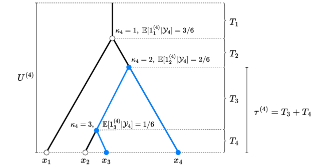
Figure 1: A pure–birth tree, stopped just before the fifth speciation event, illustrating the various coalescent components we consider. We have four tips, $n=4$, and we “randomly sample” tips $x_{3}$ and $x_{4}$, and $\tau^{(4)}$ is their coalescent time. The interspeciation times, $T_{i}$s are distributed as $T_{i}\sim\exp(i)$ in our case. The pairs $\{(x_{1},x_{2}),(x_{1},x_{3}),(x_{1},x_{4})\}$ coalesced at $\kappa_{n}=1$; at $\kappa_{n}=2$ the pairs $\{(x_{2},x_{4}),(x_{3},x_{4})\}$; and at $\kappa_{n}=3$ only the pairs $\{(x_{2},x_{3})\}$.

Y3 Summary of results concerning moments of heights of the pure–birth tree

In this section we collect a number of key first two moment properties of $U^{(n)}$, $\tau^{(n)}$, and $\operatorname{E}\left[\tau^{(n)}|\mathcal{Y}_{n}\right]$. Some of them can be found in the literature, and some we prove here. These, and related formulæ are needed when proving properties of processes evolving on a pure–birth tree, central limit theorems [Bartoszek and Sagitov, 2015a; Bartoszek, 2020; Bartoszek and Erhardsson, 2021], the sum of branch lengths [Bartoszek, 2014], or the so–called cophenetic index [Sagitov and Bartoszek, 2012; Bartoszek, 2018].

1. $\operatorname{E}\left[U^{(n)}\right]=H_{n,1}$ [e.g., Sagitov and Bartoszek, 2012, but this is essentially common knowledge];

2. $U^{(n)}-\log n$ has a Gumbel limiting distribution [Bartoszek and Sagitov, 2015a];

3. $\operatorname{E}\left[U^{(n)^{2}}\right]=H_{n,1}^{2}+H_{n,2}$ (setting $k=0$ after Eq. $(8)$ on p. $74$ in [Bartoszek and Sagitov, 2015b], or Ex. Y4.1, but this is essentially common knowledge);

4. $\operatorname{E}\left[\tau^{(n)}\right]=\frac{n+1}{n-1}H_{n,1}-\frac{2n}{n-1}$ [Sagitov and Bartoszek, 2012];

5. $\operatorname{E}\left[U^{(n)}-\tau^{(n)}\right]=2(n-H_{n,1})/(n-1)$ [Sagitov and Bartoszek, 2012];

6. $\operatorname{E}\left[U^{(n)}(U^{(n)}-\tau^{(n)})\right]=\frac{2n}{n-1}\left(H_{n,1}+H_{n,2}-1-n^{-1}H_{n,1}^{2}\right)$ (Lemma Y4.3);

7. $\operatorname{E}\left[U^{(n)}(U^{(n)}-\operatorname{E}\left[\tau^{(n)}|\mathcal{Y}_{n}\right])\right]=\frac{2n}{n-1}\left(H_{n,1}+H_{n,2}-1-n^{-1}H_{n,1}^{2}\right)$ (Lemma Y4.4);

8. $\operatorname{E}\left[\tau^{(n)^{2}}\right]=\frac{n+1}{n-1}\left((H_{n,1}-2)^{2}+H_{n,2}\right)-\frac{4}{n-1}$ (Ex. Y4.2);

9. $\operatorname{E}\left[(U^{(n)}-\tau^{(n)})^{2}\right]=\frac{4n+2}{n-1}H_{n,2}-\frac{2H_{n,1}^{2}}{n-1}-\frac{4H_{n,1}}{n-1}$ (Appendix A in [Bartoszek and Sagitov, 2015a], p. $35$ in [Bartoszek, 2018] and Lemma Y4.1 for the final simplified form);

10. $\operatorname{E}\left[\operatorname{E}\left[\tau^{(n)}|\mathcal{Y}_{n}\right]^{2}\right]=H_{n,1}^{2}-4H_{n,1}-\frac{5H_{n,2}}{3}+7+\frac{4H_{n,1}^{2}}{n}+\Theta(n^{-1}\ln n)$
    (Lemma Y4.6);

11. $\operatorname{E}\left[(U^{(n)}-\operatorname{E}\left[\tau^{(n)}|\mathcal{Y}_{n}\right])^{2}\right]=\frac{4}{3}H_{n,2}+3-8n^{-1}H_{n,1}+\Theta(n^{-1})\xrightarrow{n\to\infty}\frac{2\pi^{2}}{9}+3,$ as $n\to\infty$ (Lemma Y4.5);

12. $\operatorname{E}\left[(\tau^{(n)}-\operatorname{E}\left[\tau^{(n)}|\mathcal{Y}_{n}\right])^{2}\right]=\operatorname{E}\left[((U^{(n)}-\tau^{(n)})-(U^{(n)}-\operatorname{E}\left[\tau^{(n)}|\mathcal{Y}_{n}\right]))^{2}\right]\\ =\frac{8}{3}H_{n,2}-3-\frac{2H_{n,1}^{2}}{(n-1)}+\Theta(n^{-1}\ln n)\xrightarrow{n\to\infty}\frac{4\pi^{2}}{9}-3$ (Lemma Y4.7).

We can see that the shared path length, $U^{(n)}-\tau^{(n)}$, for a random pair of tip species, has mean value converging to $2$ and variance to $4(\pi^{2}/6-1)$. This means that we expect that on average the shared path length between a pair of species is small compared the tree’s height, which has expectation behaving as $\ln n$ and variance converging to $\pi^{2}/6$.

As already mentioned, these heights are related to important tree statistics. For example the total cophenetic index (generalized to trees with branch lengths) will equal $\binom{n}{2}\left(U^{(n)}-\operatorname{E}\left[\tau^{(n)}|\mathcal{Y}_{n}\right]\right)$, and in fact this was discussed and exploited by Bartoszek [2018]. Hence, e.g., from Lemma Y4.5 we can obtain the second moment, or combining Lemma Y4.5 with $\operatorname{E}\left[U^{(n)}-\tau^{(n)}\right]$ easily gives the variance.

Y4 Moments of heights of the pure–birth tree

Theorem Y4.1 (Appendix A in Bartoszek and Sagitov [2015a])

Define the set of integer valued vectors

$$\mathcal{A}_{m}=\{\mathbf{k}:\sum\limits_{i=1}^{m}k_{i}i=m\},$$

i.e., $\mathcal{A}_{m}$ is the set of all possible ways to represent $m$ as a sum of positive integers. The $m$–th moment of the tree height of a Yule tree with speciation rate $1$ is

$$\operatorname{E}\left[\left(U^{(n)}\right)^{m}\right]=\sum\limits_{\mathbf{k}\in\mathcal{A}_{m}}c_{\mathbf{k}}\prod\limits_{i=1}^{m}H_{n,i}^{k_{i}},$$ (Y4.1)

where for a non–negative integer valued vector $\mathbf{k}=(k_{1},k_{2},\ldots)$, such that $m=\sum_{i=1}^{m}k_{i}i$ we define $c_{\mathbf{k}}$ recursively as

$$c_{\mathbf{k}}=c_{\mathbf{k},0}+\sum\limits_{j=1}^{m-1}(j(k_{j}+1))c_{\mathbf{k},j},$$ (Y4.2)

and

$$\begin{array}[]{c}c_{\mathbf{k},0}=c_{(k_{1}-1,k_{2},k_{3},\ldots)}\\ c_{\mathbf{k},j}=c_{(k_{1},\ldots,k_{j}+1,k_{j+1}-1,\ldots)},~j\geq 1.\end{array}$$

The boundary conditions for Eq. (Y4.2) are

1. $c_{\mathbf{k}}=0$ if all $k_{i}=0$ or one of the coordinates of $\mathbf{k}$ is negative,

2. $c_{\mathbf{k}}=1$ if $k_{1}\geq 1$ and all other $k_{i}=0$.

Proof The proof of this theorem can be found in Appendix A in Bartoszek and Sagitov [2015a]. For the convenience of the reader, especially as its steps are helpful in proving the next Thm. Y4.2, we provide here a full detailed proof of it. One can find in KBarSSag2015aart Lemma $3$ that the Laplace transform of the height of the Yule tree is

$$\operatorname{E}\left[e^{-xU^{(n)}}\right]=b_{n,x}.$$

We will use the property that for a random variable $Z$, with Laplace transform $\mathcal{L}_{Z}(x)$, its $m$–th moment is obtained as

$$\operatorname{E}\left[Z^{m}\right]=(-1)^{m}\frac{\mathrm{d}^{m}\mathcal{L}_{Z}}{\mathrm{d}x^{m}}|_{x=0}.$$

We introduce the notation (for a fixed $n$)

$$A(x)=b_{n,x}/n!=\frac{1}{x+1}\cdot\ldots\cdot\frac{1}{x+n},~~b_{m}(x)=\frac{1}{(x+1)^{m}}+\ldots+\frac{1}{(x+n)^{m}}$$

and also the vector $\mathbf{b}_{m}(x)=(b_{1}(x),\ldots,b_{m}(x))$. We can immediately notice that $A(0)=1/n!$ and $b_{m}(0)=H_{n,m}$. The first and second derivatives of $A(x)$ are $A^{\prime}(x)=-A(x)b_{1}(x)$ and $A^{\prime\prime}(x)=A(x)(b_{1}^{2}(x)+b_{2}(x))$, notice that $b^{\prime}_{m}(x)=-mb_{m+1}(x)$. We also introduce the multi–index notation $\mathbf{b}_{m}(x)^{\mathbf{k}}=b_{1}(x)^{k_{1}}\cdot\ldots\cdot b_{m}(x)^{k_{m}}$. One then shows inductively that

$$\frac{\mathrm{d}^{m}}{\mathrm{d}x^{m}}A(x)=(-1)^{m}A(x)\sum\limits_{\mathbf{k}\in\mathcal{A}_{m}}c_{\mathbf{k}}\mathbf{b}_{m}(x)^{\mathbf{k}}.$$ (Y4.3)

We can see directly that Eq. (Y4.3) holds for $m=1$. Assume that it holds till $m$ and the $m+1$st derivative is

$$\begin{array}[]{l}\frac{\mathrm{d}^{m+1}}{\mathrm{d}x^{m}}A(x)=\left(\frac{\mathrm{d}^{m}}{\mathrm{d}x^{m}}A(x)\right)^{\prime}=\left((-1)^{m}A(x)\sum\limits_{\mathbf{k}\in\mathcal{A}_{m}}c_{\mathbf{k}}\mathbf{b}_{m}(x)^{\mathbf{k}}\right)^{\prime}\\ =(-1)^{m}\left(A^{\prime}(x)\sum\limits_{\mathbf{k}\in\mathcal{A}_{m}}c_{\mathbf{k}}\mathbf{b}_{m}(x)^{\mathbf{k}}+A(x)\sum\limits_{\mathbf{k}\in\mathcal{A}_{m}}c_{\mathbf{k}}(\mathbf{b}_{m}(x)^{\mathbf{k}})^{\prime}\right)\\ =(-1)^{m+1}A(x)\left(\sum\limits_{\mathbf{k}\in\mathcal{A}_{m}}c_{\mathbf{k}}\left(\mathbf{b}_{m}(x)^{(k_{1}+1,k_{2},\ldots)}+\sum\limits_{i=1}^{m}ik_{i}\mathbf{b}_{m+1}^{(k_{1},\ldots,k_{i}-1,k_{i+1}+1,\ldots)}\right)\right).\end{array}$$

As, $k_{1}+i(k_{i}-1)+(i+1)(k_{i+1}+1)+\ldots=k_{1}+ik_{i}+(i+1)k_{i+1}+\ldots+i+1-i=k_{1}+ik_{i}+(i+1)k_{i+1}+\ldots+1=m+1$, for any given $\mathbf{k}\in\mathcal{A}_{m+1}$ we will obtain in front of $\mathbf{b}_{m+1}(x)^{\mathbf{k}}$ the coefficient

$$c_{(k_{1}-1,k_{2},\ldots)}+\sum\limits_{i=1}^{m}c_{(k_{1},\ldots,k_{i}+1,k_{i+1}-1,\ldots)}i(k_{i}+1)\equiv c_{\mathbf{k},0}+\sum\limits_{i=1}^{m}c_{\mathbf{k},i}i(k_{i}+1),$$

as desired. Evaluating the derivative at $0$ we obtain

$$\frac{\mathrm{d}^{m}}{\mathrm{d}x^{m}}A(x)|_{x=0}=(-1)^{m}A(0)\sum\limits_{\mathbf{k}\in\mathcal{A}_{m}}c_{\mathbf{k}}\mathbf{b}_{m}(0)^{\mathbf{k}}=(-1)^{m}\frac{1}{n!}\sum\limits_{\mathbf{k}\in\mathcal{A}_{m}}c_{\mathbf{k}}\prod\limits_{i=1}^{m}H_{n,i}^{k_{i}}.$$

To obtain the final statement recall that $\operatorname{E}\left[e^{-xU^{(n)}}\right]=b_{n,x}=n!A(x)$.

$\Box$

Example Y4.1

We recover here the first two moments, $m=1,2$, for $U^{(n)}$. We first need to find $c_{\mathbf{k}}$ for $\mathbf{k}\in\mathcal{A}_{1},\mathcal{A}_{2}$. The only $\mathbf{k}$ vectors that need to be considered are $\mathbf{v}_{1}=(1,0,0,\ldots)$, $\mathbf{v}_{2}=(2,0,0,\ldots)$, $\mathbf{v}_{3}=(0,1,0,0\ldots)$. We have directly from the boundary conditions that $c_{\mathbf{v}_{1}}=1$. We calculate for $\mathbf{v}_{2}$ $c_{\mathbf{v}_{2}}=c_{\mathbf{v}_{2},0}+1(2+1)c_{\mathbf{v}_{2},1}$,

$$\begin{array}[]{l}c_{\mathbf{v}_{2},0}=c_{(1,0,\ldots)}=1,\\ c_{\mathbf{v}_{2},1}=c_{(3,-1,0,\ldots)}=0,\end{array}$$

resulting in $c_{\mathbf{v}_{2}}=1$. For $\mathbf{v}_{3}$ $c_{\mathbf{v}_{3}}=c_{\mathbf{v}_{3},0}+1(0+1)c_{\mathbf{v}_{2},1}$,

$$\begin{array}[]{l}c_{\mathbf{v}_{3},0}=c_{(-1,1,\ldots)}=0,\\ c_{\mathbf{v}_{3},1}=c_{(1,0,0,\ldots)}=1,\end{array}$$

resulting in $c_{\mathbf{v}_{3}}=1$. From Eq. (Y4.1) we have

$$\begin{array}[]{l}\operatorname{E}\left[U^{(n)}\right]=\sum\limits_{\mathbf{k}\in\mathcal{A}_{1}}c_{\mathbf{k}}\prod\limits_{i=1}^{1}H_{n,i}^{k_{i}}=c_{\mathbf{v}_{1}}H_{n,1}^{1}=H_{n,1},\\ \operatorname{E}\left[U^{(n)^{2}}\right]=\sum\limits_{\mathbf{k}\in\mathcal{A}_{2}}c_{\mathbf{k}}\prod\limits_{i=1}^{2}H_{n,i}^{k_{i}}=c_{\mathbf{v}_{2}}H_{n,1}^{2}H_{n,2}^{0}+c_{\mathbf{v}_{3}}H_{n,1}^{0}H_{n,2}^{1}=H_{n,1}^{2}+H_{n,2}.\end{array}$$

Theorem Y4.2 (Appendix A Bartoszek and Sagitov [2015a])

The $m$–th moment of the time to coalescent of a random pair of tips in a Yule tree with speciation rate $1$, with the same notation as in Thm. Y4.1, is

$$\operatorname{E}\left[\left(\tau^{(n)}\right)^{m}\right]=(-1)^{m+1}\frac{2}{(n-1)}m!+\frac{n+1}{n-1}\sum\limits_{\mathbf{k}\in\mathcal{A}_{m}}c_{\mathbf{k}}\left(\prod\limits_{\begin{array}[]{c}i=1\\ i\mathrm{~even}\end{array}}^{m}H_{n,i}^{k_{i}}\right)\left(\prod\limits_{\begin{array}[]{c}i=1\\ i\mathrm{~odd}\end{array}}^{m}(H_{n,i}-2)^{k_{i}}\right).$$ (Y4.4)

Proof For the convenience of the reader we provide a full detailed proof here (Bartoszek and Sagitov [2015a] considered the joint moment $\operatorname{E}\left[(U^{(n)}-\tau^{(n)})^{m}\left(\tau^{(n)}\right)^{r}\right]$). The proof will come along the lines of the proof of Thm. Y4.1. We first recall that the Laplace transform for $\tau^{(n)}$ is (KBarSSag2015aart Lemma $3$)

$$\operatorname{E}\left[e^{-x\tau^{(n)}}\right]=\frac{2-(n+1)(x+1)b_{n,x}}{(n-1)(x-1)}=\frac{2}{(n-1)}\frac{1}{(x-1)}-\left(\frac{n+1}{n-1}\right)\frac{(x+1)}{(x-1)}b_{n,x}.$$ (Y4.5)

We are interested in the behaviour around $0$ so the singularity at $x=1$ is not relevant here. The $m$–th derivative of $(x-1)^{-1}$ is

$$\left(\frac{1}{x-1}\right)^{(m)}=(-1)^{m}\frac{m!}{(x-1)^{m+1}}.$$

One needs to now consider the $m$–th derivative of $(x+1)b_{n,x}/(x-1)$. Define now $\hat{A}(x)=(x+1)A(x)/(x-1)$ and

$$\hat{b}_{1}(x)=b_{1}(x)+2\frac{1}{(x+1)(x-1)}.$$

The $m$–th derivative of $1/((x-1)(x+1))$ is

$$\left(\frac{1}{(x-1)(x+1)}\right)^{(m)}=(-1)^{m}m!\sum\limits_{i=1}^{m+1}\frac{1}{(x+1)^{i}(x-1)^{m+2-i}}.$$ (Y4.6)

Defining generally,

$$\begin{array}[]{l}\hat{b}_{m}(x)=b_{m}(x)+2\sum\limits_{i=1}^{m}\frac{1}{(x+1)^{i}(x-1)^{m+1-i}}=b_{m}(x)+\left(\frac{1}{(x-1)^{m}}-\frac{1}{(x+1)^{m}}\right).\end{array}$$

The second component,

$$\sum\limits_{i=1}^{m}\frac{1}{(x+1)^{i}(x-1)^{m+1-i}}=\frac{1}{2}\left(\frac{1}{(x-1)^{m}}-\frac{1}{(x+1)^{m}}\right),$$

can be checked by induction on $m$. Hence, we can see that $\hat{b}_{m+1}^{\prime}(x)=-m\hat{b}_{m+1}(x)$. Now we turn to calculating the $m$–th derivative of $(\hat{A}(x))^{(m)}$. We have

$$\begin{array}[]{l}\hat{A}^{\prime}(x)=\left(\frac{x+1}{x-1}\right)^{\prime}A(x)+\frac{x+1}{x-1}A^{\prime}(x)=(-1)\left(2\frac{1}{(x-1)(x+1)}+b_{1}(x)\right)\hat{A}(x)=(-1)\hat{A}(x)\hat{b}_{1}(x).\end{array}$$

Hence, as $\hat{A}^{\prime}(x)=(-1)\hat{b}_{1}(x)\hat{A}(x)$ and $\hat{b}_{m+1}^{\prime}(x)=-m\hat{b}_{m+1}(x)$ we have the same situation as in Thm. Y4.1. Therefore, we may directly write

$$\frac{\mathrm{d}^{m}}{\mathrm{d}x^{m}}\hat{A}(x)=(-1)^{m}\hat{A}(x)\sum\limits_{\mathbf{k}\in\mathcal{A}_{m}}c_{\mathbf{k}}\mathbf{\hat{b}}_{m}(x)^{\mathbf{k}}.$$ (Y4.7)

Now, we obtain that the $m$–th derivative of the Laplace transform of $\tau^{(n)}$ will be

$$\begin{array}[]{l}\left(\operatorname{E}\left[e^{-x\tau^{(n)}}\right]\right)^{(m)}=\frac{2}{(n-1)}\left(\frac{1}{(x-1)}\right)^{(m)}-\left(\frac{n+1}{n-1}\right)\left(\frac{(x+1)}{(x-1)}b_{n,x}\right)^{(m)}\\ =\frac{2}{(n-1)}\left(\frac{1}{(x-1)}\right)^{(m)}-\left(\frac{n+1}{n-1}\right)n!\hat{A}(x)^{(m)}\\ =(-1)^{m}\left(\frac{2}{(n-1)}\frac{m!}{(x-1)^{m+1}}-\frac{(n+1)!}{n-1}\hat{A}(x)\sum\limits_{\mathbf{k}\in\mathcal{A}_{m}}c_{\mathbf{k}}\mathbf{\hat{b}}_{m}(x)^{\mathbf{k}}\right).\end{array}$$

To evaluate the derivative at $0$ we notice that $\hat{A}(0)=-A(0)=1/n!$ and

$$\begin{array}[]{l}\hat{b}_{m}(0)=b_{m}(0)+((-1)^{m}-1)=H_{n,m}+((-1)^{m}-1)\\ =\left\{\begin{array}[]{lc}H_{n,m}&m\mathrm{~is~even},\\ H_{n,m}-2&m\mathrm{~is~odd}.\\ \end{array}\right.\end{array}$$

Therefore,

$$\operatorname{E}\left[\tau^{(n)^{m}}\right]=(-1)^{m+1}\frac{2}{(n-1)}m!+\frac{n+1}{n-1}\sum\limits_{\mathbf{k}\in\mathcal{A}_{m}}c_{\mathbf{k}}\left(\prod\limits_{\begin{array}[]{c}i=1\\ i\mathrm{~even}\end{array}}^{m}H_{n,i}^{k_{i}}\right)\left(\prod\limits_{\begin{array}[]{c}i=1\\ i\mathrm{~odd}\end{array}}^{m}(H_{n,i}-2)^{k_{i}}\right).$$

$\Box$

Example Y4.2

We recover here the first two moments $m=1,2$, for $\tau^{(n)}$. We have the same $c_{\mathbf{v}_{1}}$, $c_{\mathbf{v}_{2}}$ and $c_{\mathbf{v}_{3}}$ as in Example Y4.1. From Eq. (Y4.4) we have

$$\begin{array}[]{l}\operatorname{E}\left[\tau^{(n)}\right]=(-1)^{1+1}\frac{2}{(n-1)}1!+\frac{n+1}{n-1}\sum\limits_{\mathbf{k}\in\mathcal{A}_{1}}c_{\mathbf{k}}\left(\prod\limits_{\begin{array}[]{c}i=1\\ i\mathrm{~even}\end{array}}^{1}H_{n,i}^{k_{i}}\right)\left(\prod\limits_{\begin{array}[]{c}i=1\\ i\mathrm{~odd}\end{array}}^{1}(H_{n,i}-2)^{k_{i}}\right)\\ =\frac{2}{n-1}+\frac{n+1}{n-1}c_{\mathbf{v}_{1}}(H_{n,i}-2)^{1}=\frac{2}{n-1}+\frac{n+1}{n-1}(H_{n,i}-2),\\ \operatorname{E}\left[\tau^{(n)^{2}}\right]=(-1)^{2+1}\frac{2}{(n-1)}2!+\frac{n+1}{n-1}\sum\limits_{\mathbf{k}\in\mathcal{A}_{2}}c_{\mathbf{k}}\left(\prod\limits_{\begin{array}[]{c}i=1\\ i\mathrm{~even}\end{array}}^{2}H_{n,i}^{k_{i}}\right)\left(\prod\limits_{\begin{array}[]{c}i=1\\ i\mathrm{~odd}\end{array}}^{2}(H_{n,i}-2)^{k_{i}}\right)\\ =\frac{(-4)}{(n-1)}+\frac{n+1}{n-1}\left(c_{\mathbf{v}_{2}}H_{n,2}^{0}(H_{n,1}-2)^{2}+c_{\mathbf{v}_{3}}H_{n,2}^{1}(H_{n,1}-2)^{0}\right)\\ =\frac{n+1}{n-1}\left((H_{n,1}-2)^{2}+H_{n,2}\right)-\frac{4}{(n-1)}.\end{array}$$

Lemma Y4.1 (See also the proof of Thm. $5.1$ in [Bartoszek, 2018])

For a Yule tree with speciation rate $\lambda=1$ we have

$$\operatorname{E}\left[(U^{(n)}-\tau^{(n)})^{2}\right]=\frac{4n+2}{n-1}H_{n,2}-\frac{2H_{n,1}^{2}}{n-1}-\frac{4H_{n,1}}{n-1}$$ (Y4.8)

Proof We will derive the second moment from the general joint moments formula, with an alternative proof in Appendix YB: Direct, alternative proofs of Lemmata Y4.1 and Y4.5. Using the same notation as in Thm. Y4.1, we first recall from KBarSSag2015aart Appendix A the general joint moment formula (setting $r=0$)

$$\operatorname{E}\left[(U^{(n)}-\tau^{(n)})^{m}\right]=(-1)^{m}\frac{2(n+1)}{(n-1)}\sum\limits_{j=1}^{n-1}\frac{1}{(j+1)(j+2)}\left(\sum\limits_{\mathbf{k}\in\mathcal{A}_{m}}c_{\mathbf{k}}\prod\limits_{i=1}^{m}H_{j,i}^{k_{i}}\right).$$ (Y4.9)

Setting $m=2$, recalling Example Y4.1, and using Lemmata LABEL:HarXiv-lemSumHi2i1i2 and LABEL:HarXiv-lemSumHisqi1i2app we may write

$$\begin{array}[]{l}\operatorname{E}\left[(U^{(n)}-\tau^{(n)})^{2}\right]=\frac{2(n+1)}{(n-1)}\sum\limits_{j=1}^{n-1}\frac{1}{(j+1)(j+2)}\left(\sum\limits_{\mathbf{k}\in\mathcal{A}_{2}}c_{\mathbf{k}}\prod\limits_{i=1}^{2}H_{j,i}^{k_{i}}\right)\\ =\frac{2(n+1)}{(n-1)}\sum\limits_{j=1}^{n-1}\frac{1}{(j+1)(j+2)}\left(c_{\mathbf{v}_{2}}H_{j,1}^{2}H_{j,2}^{0}+c_{\mathbf{v}_{3}}H_{j,1}^{0}H_{j,2}^{1}\right)=\frac{2(n+1)}{(n-1)}\left(\sum\limits_{j=1}^{n-1}\frac{H_{j,1}^{2}}{(j+1)(j+2)}+\sum\limits_{j=1}^{n-1}\frac{H_{j,2}}{(j+1)(j+2)}\right)\\ \stackrel{{\scriptstyle\mathrm{Lemmata~\ref{HarXiv-lemSumHi2i1i2},\ref{HarXiv-lemSumHisqi1i2app}}}}{{=}}\frac{2(n+1)}{(n-1)}\left(H_{n,2}+\frac{(n-1)^{2}+n-1-1}{n^{2}}-2\frac{H_{n-1,1}}{n}-\frac{H_{n-1,1}^{2}}{n+1}+\frac{n}{n+1}\left(H_{n,2}-1\right)\right)\\ =\frac{4n+2}{n-1}H_{n,2}-\frac{4H_{n,1}}{n-1}-\frac{2H_{n,1}^{2}}{n-1}.\end{array}$$

This equation is compared with simulations in Fig. 2.

$\Box$

Lemma Y4.2

For a Yule tree with speciation rate $\lambda=1$ we have

$$\operatorname{E}\left[U^{(n)}\tau^{(n)}\right]=\frac{n+1}{n-1}\left(H_{n,1}^{2}-H_{n,2}\right)-\frac{2n}{n-1}\left(H_{n,1}-1\right).$$ (Y4.10)

Proof We can calculate the cross–moment using Examples Y4.1, Y4.2, and Lemma Y4.1. We have

$$\begin{array}[]{l}\operatorname{E}\left[U^{(n)}\tau^{(n)}\right]=\frac{1}{2}\left(\operatorname{E}\left[U^{(n)^{2}}\right]+\operatorname{E}\left[\tau^{(n)^{2}}\right]-\operatorname{E}\left[(U^{(n)}-\tau^{(n)})^{2}\right]\right)\\ =\frac{1}{2}\left(H_{n,1}^{2}+H_{n,2}+\frac{n+1}{n-1}\left((H_{n,1}-2)^{2}+H_{n,2}\right)-\frac{4}{(n-1)}-\frac{4n+2}{n-1}H_{n,2}+\frac{4H_{n,1}}{n-1}+\frac{2H_{n,1}^{2}}{n-1}\right)\\ =\frac{n+1}{n-1}\left(H_{n,1}^{2}-H_{n,2}\right)-\frac{2n}{n-1}\left(H_{n,1}-1\right).\end{array}$$

This equation is compared with simulations in Fig. 2.

$\Box$

Lemma Y4.3

For a Yule tree with speciation rate $\lambda=1$ we have

$$\operatorname{E}\left[U^{(n)}(U^{(n)}-\tau^{(n)})\right]=\frac{2n}{n-1}\left(H_{n,1}+H_{n,2}-1-n^{-1}H_{n,1}^{2}\right).$$ (Y4.11)

Proof Using Lemma Y4.2 and Example Y4.1

$$\begin{array}[]{l}\operatorname{E}\left[U^{(n)}(U^{(n)}-\tau^{(n)})\right]=\operatorname{E}\left[U^{(n)^{2}}\right]-\operatorname{E}\left[U^{(n)}\tau^{(n)}\right]\\ =H_{n,1}^{2}+H_{n,2}-\frac{n+1}{n-1}\left(H_{n,1}^{2}-H_{n,2}\right)+\frac{2n}{n-1}\left(H_{n,1}-1\right)\\ =\frac{2n}{n-1}\left(H_{n,1}+H_{n,2}-1-n^{-1}H_{n,1}^{2}\right).\end{array}$$

This equation is compared with simulations in Fig. 2.

$\Box$

Lemma Y4.4

For a Yule tree with speciation rate $\lambda=1$ we have

$$\operatorname{E}\left[U^{(n)}(U^{(n)}-\operatorname{E}\left[\tau^{(n)}|\mathcal{Y}_{n}\right])\right]=\frac{2n}{n-1}\left(H_{n,1}+H_{n,2}-1-n^{-1}H_{n,1}^{2}\right).$$ (Y4.12)

Proof

$$\begin{array}[]{l}\operatorname{E}\left[U^{(n)}(U^{(n)}-\operatorname{E}\left[\tau^{(n)}|\mathcal{Y}_{n}\right])\right]=\operatorname{E}\left[\operatorname{E}\left[U^{(n)}(U^{(n)}-\tau^{(n)}|\mathcal{Y}_{n})\right]\right]=\operatorname{E}\left[U^{(n)}(U^{(n)}-\tau^{(n)})\right].\end{array}$$

This equation is compared with simulations in Fig. 2.

$\Box$

Lemma Y4.5

For a Yule tree with speciation rate $\lambda=1$ we have

$$\begin{array}[]{l}\operatorname{E}\left[(U^{(n)}-\operatorname{E}\left[\tau^{(n)}|\mathcal{Y}_{n}\right])^{2}\right]=\frac{4}{3}H_{n,2}+3-8n^{-1}H_{n,1}+\Theta(n^{-1})\xrightarrow{n\to\infty}\frac{2\pi^{2}}{9}+3.\end{array}$$ (Y4.13)

Proof We have from the second formula in KBar2018art Thm. $6.4$

$$\begin{array}[]{l}\operatorname{Var}\left[U^{(n)}-\operatorname{E}\left[\tau^{(n)}|\mathcal{Y}_{n}\right]\right]=\frac{12n^{2}(n^{2}-6n-4)H_{n-1,2}-9n^{4}+102n^{3}+51n^{2}-24nH_{n-1,1}-72n-72}{9n^{2}(n-1)^{2}}\end{array}$$

and from this we obtain [recalling that $\operatorname{E}\left[U^{(n)}-\tau^{(n)}\right]=2(n-H_{n,1})/(n-1)$, Sagitov and Bartoszek, 2012]

$$\begin{array}[]{l}\operatorname{E}\left[\left(U^{(n)}-\operatorname{E}\left[\tau^{(n)}|\mathcal{Y}_{n}\right]\right)^{2}\right]=\operatorname{Var}\left[U^{(n)}-\operatorname{E}\left[\tau^{(n)}|\mathcal{Y}_{n}\right]\right]+\left(\operatorname{E}\left[U^{(n)}-\operatorname{E}\left[\tau^{(n)}|\mathcal{Y}_{n}\right]\right]\right)^{2}\\ =\operatorname{Var}\left[U^{(n)}-\operatorname{E}\left[\tau^{(n)}|\mathcal{Y}_{n}\right]\right]+\left(\operatorname{E}\left[U^{(n)}-\tau^{(n)}\right]\right)^{2}=\operatorname{Var}\left[U^{(n)}-\operatorname{E}\left[\tau^{(n)}|\mathcal{Y}_{n}\right]\right]+\left(\frac{2(n-H_{n,1})}{n-1}\right)^{2}\\ =\frac{12n^{4}H_{n-1,2}-72n^{3}H_{n-1,2}-48n^{2}H_{n-1,2}-9n^{4}+102n^{3}+51n^{2}-24nH_{n-1,1}-72n-72}{9n^{2}(n-1)^{2}}+\frac{36n^{4}-72n^{3}H_{n,1}+36n^{2}H_{n,1}^{2}}{9n^{2}(n-1)^{2}}\\ =\frac{12n^{4}H_{n,2}-12n^{2}-72n^{3}H_{n,2}+72n-48n^{2}H_{n,2}+48-9n^{4}+102n^{3}+51n^{2}-24nH_{n-1,1}-72n-72}{9n^{2}(n-1)^{2}}+\frac{36n^{4}-72n^{3}H_{n,1}+36n^{2}H_{n,1}^{2}}{9n^{2}(n-1)^{2}}\\ =\frac{12n^{4}H_{n,2}+27n^{4}-72n^{3}H_{n,1}-72n^{3}H_{n,2}+102n^{3}+36n^{2}H_{n,1}^{2}-48n^{2}H_{n,2}+39n^{2}-24nH_{n,1}}{9n^{2}(n-1)^{2}}.\end{array}$$

We can simplify the above and obtain the asymptotics

$$\begin{array}[]{l}\operatorname{E}\left[\left(U^{(n)}-\operatorname{E}\left[\tau^{(n)}|\mathcal{Y}_{n}\right]\right)^{2}\right]=\frac{4n^{3}H_{n,2}+9n^{3}-24n^{2}H_{n,1}-24n^{2}H_{n,2}+34n^{2}+12nH_{n,1}^{2}-16nH_{n,2}+13n-8H_{n,1}}{3n(n-1)^{2}}\\ \xlongrightarrow{n\to\infty}\frac{2\pi^{2}}{9}+3\approx 5.19325.\end{array}$$ (Y4.14)

This key equation is compared with simulations in Fig. 2. In Appendix YB: Direct, alternative proofs of Lemmata Y4.1 and Y4.5 we show an alternative, direct proof of this lemma.

$\Box$

Lemma Y4.6

For a Yule tree with speciation rate $\lambda=1$ we have

$$\operatorname{E}\left[\operatorname{E}\left[\tau^{(n)}|\mathcal{Y}_{n}\right]^{2}\right]=H_{n,1}^{2}-4H_{n,1}-\frac{5H_{n,2}}{3}+7+\frac{4H_{n,1}^{2}}{n}+\Theta(n^{-1}\ln n).$$ (Y4.15)

Proof We may write

$$\begin{array}[]{l}\operatorname{E}\left[\operatorname{E}\left[\tau^{(n)}|\mathcal{Y}_{n}\right]^{2}\right]=\operatorname{E}\left[\left(U^{(n)}-U^{(n)}+\operatorname{E}\left[\tau^{(n)}|\mathcal{Y}_{n}\right]\right)^{2}\right]\\ =\operatorname{E}\left[U^{(n)^{2}}\right]-2\operatorname{E}\left[U^{(n)}\left(U^{(n)}-\operatorname{E}\left[\tau^{(n)}|\mathcal{Y}_{n}\right]\right)\right]+\operatorname{E}\left[\left(U^{(n)}-\operatorname{E}\left[\tau^{(n)}|\mathcal{Y}_{n}\right]\right)^{2}\right]\\ \stackrel{{\scriptstyle Lemmata~\ref{lemUnUnmETaunYn},\ref{lemUnmETaunYn2}}}{{=}}H_{n,1}^{2}+H_{n,2}-\frac{4n}{n-1}\left(H_{n,1}+H_{n,2}-1-n^{-1}H_{n,1}^{2}\right)+\frac{4n^{2}H_{n,2}}{3(n-1)^{2}}\\ +\frac{3n^{2}}{(n-1)^{2}}-\frac{8nH_{n,1}}{(n-1)^{2}}-\frac{8nH_{n,2}}{(n-1)^{2}}+\frac{34n}{3(n-1)^{2}}+\frac{4H_{n,1}^{2}}{(n-1)^{2}}-\frac{16H_{n,2}}{3(n-1)^{2}}+\frac{13}{3(n-1)^{2}}-\frac{8H_{n,1}}{3n(n-1)^{2}}\\ =H_{n,1}^{2}-4H_{n,1}-\frac{5H_{n,2}}{3}+7+\frac{4H_{n,1}^{2}}{n}-\frac{12H_{n,1}}{n-1}-\frac{28H_{n,2}}{3(n-1)}+\frac{64}{3(n-1)}+\frac{8H_{n,1}^{2}}{(n-1)^{2}}\\ -\frac{8H_{n,1}}{(n-1)^{2}}-\frac{12H_{n,2}}{(n-1)^{2}}+\frac{56}{3(n-1)^{2}}-\frac{4H_{n,1}^{2}}{n(n-1)^{2}}-\frac{8H_{n,1}}{3n(n-1)^{2}}.\end{array}$$

This equation is compared with simulations in Fig. 2.

$\Box$

Lemma Y4.7

For a Yule tree with speciation rate $\lambda=1$ we have

$$\begin{array}[]{l}\operatorname{E}\left[(\tau^{(n)}-\operatorname{E}\left[\tau^{(n)}|\mathcal{Y}_{n}\right])^{2}\right]=\operatorname{E}\left[\left(\left(U^{(n)}-\tau^{(n)}\right)-\left(U^{(n)}-\operatorname{E}\left[\tau^{(n)}|\mathcal{Y}_{n}\right]\right)\right)^{2}\right]\\ =\frac{8}{3}H_{n,2}-3-\frac{2H_{n,1}^{2}}{(n-1)}+\Theta(n^{-1}\ln n)\xrightarrow{n\to\infty}\frac{4\pi^{2}}{9}-3.\end{array}$$ (Y4.16)

Proof We begin by rewriting

$$\begin{array}[]{l}\operatorname{E}\left[\left(\tau^{(n)}-\operatorname{E}\left[\tau^{(n)}|\mathcal{Y}_{n}\right]\right)^{2}\right]=\operatorname{E}\left[\left(\left(U^{(n)}-\tau^{(n)}\right)-\left(U^{(n)}-\operatorname{E}\left[\tau^{(n)}|\mathcal{Y}_{n}\right]\right)\right)^{2}\right]\\ =\operatorname{E}\left[\left(U^{(n)}-\tau^{(n)}\right)^{2}\right]-2\operatorname{E}\left[\left(U^{(n)}-\tau^{(n)}\right)\left(U^{(n)}-\operatorname{E}\left[\tau^{(n)}|\mathcal{Y}_{n}\right]\right)\right]+\operatorname{E}\left[\left(\operatorname{E}\left[U^{(n)}-\tau^{(n)}|\mathcal{Y}_{n}\right]\right)^{2}\right]\end{array}$$

and we recall that we know $\operatorname{E}\left[\left(U^{(n)}-\tau^{(n)}\right)^{2}\right]$ and Lemma Y4.5 gives us $\operatorname{E}\left[\left(U^{(n)}-\operatorname{E}\left[\tau^{(n)}|\mathcal{Y}_{n}\right]\right)^{2}\right]$. We then turn to considering the remaining

$$\begin{array}[]{l}\operatorname{E}\left[(\left(U^{(n)}-\tau^{(n)}\right)\left(U^{(n)}-\operatorname{E}\left[\tau^{(n)}|\mathcal{Y}_{n}\right]\right)\right]=\operatorname{E}\left[\operatorname{E}\left[(\left(U^{(n)}-\tau^{(n)}\right)\left(U^{(n)}-\operatorname{E}\left[\tau^{(n)}|\mathcal{Y}_{n}\right]\right)\right]|\mathcal{Y}_{n}\right]\\ =\operatorname{E}\left[\operatorname{E}\left[U^{(n)}-\tau^{(n)}\right]|\mathcal{Y}_{n}\operatorname{E}\left[U^{(n)}-\tau^{(n)}|\mathcal{Y}_{n}\right]\right]=\operatorname{E}\left[\left(\operatorname{E}\left[U^{(n)}-\tau^{(n)}\right]|\mathcal{Y}_{n}\right)^{2}\right]\end{array}$$ (Y4.17)

and hence can write

$$\operatorname{E}\left[\left(\left(U^{(n)}-\tau^{(n)}\right)-\left(U^{(n)}-\operatorname{E}\left[\tau^{(n)}|\mathcal{Y}_{n}\right]\right)\right)^{2}\right]=\operatorname{E}\left[\left(U^{(n)}-\tau^{(n)}\right)^{2}\right]-\operatorname{E}\left[\left(\operatorname{E}\left[U^{(n)}-\tau^{(n)}|\mathcal{Y}_{n}\right]\right)^{2}\right]$$ (Y4.18)

and plugging in our previously known values

$$\begin{array}[]{l}\operatorname{E}\left[\left(U^{(n)}-\tau^{(n)}\right)^{2}\right]-\operatorname{E}\left[\operatorname{E}\left[\left(U^{(n)}-\tau^{(n)}|\mathcal{Y}_{n}\right]\right)^{2}\right]\\ \stackrel{{\scriptstyle Lemmata~\ref{lemUnmTaun2},\ref{lemUnmETaunYn2}}}{{=}}\frac{4n+2}{n-1}H_{n,2}-\frac{2H_{n,1}^{2}}{n-1}-\frac{4H_{n,1}}{n-1}-\frac{4n^{2}H_{n,2}}{3(n-1)^{2}}-\frac{3n^{2}}{(n-1)^{2}}+\frac{8nH_{n,1}}{(n-1)^{2}}+\frac{8nH_{n,2}}{(n-1)^{2}}\\ -\frac{34n}{3(n-1)^{2}}-\frac{4H_{n,1}^{2}}{(n-1)^{2}}+\frac{16H_{n,2}}{3(n-1)^{2}}-\frac{13}{3(n-1)^{2}}+\frac{8H_{n,1}}{3n(n-1)^{2}}\\ =4H_{n,2}-\frac{4}{3}H_{n,2}+\frac{10H_{n,2}}{3(n-1)}-\frac{4H_{n,2}}{3(n-1)^{2}}-3-\frac{6}{(n-1)}-\frac{3}{(n-1)^{2}}-\frac{2H_{n,1}^{2}}{n-1}-\frac{4H_{n,1}^{2}}{(n-1)^{2}}+\frac{4H_{n,1}}{(n-1)}+\frac{8H_{n,1}}{(n-1)^{2}}\\ +\frac{8H_{n,2}}{n-1}+\frac{8H_{n,2}}{(n-1)^{2}}-\frac{34}{3(n-1)}-\frac{34}{3(n-1)^{2}}+\frac{16H_{n,2}}{3(n-1)^{2}}-\frac{13}{3(n-1)^{2}}+\frac{8H_{n,1}}{3n(n-1)^{2}}\\ =\frac{8}{3}H_{n,2}-3-\frac{2H_{n,1}^{2}}{n-1}\par+\frac{4H_{n,1}}{(n-1)}\par+\frac{34H_{n,2}}{3(n-1)}-\frac{52}{3(n-1)}\par-\frac{4H_{n,1}^{2}}{(n-1)^{2}}+\frac{8H_{n,1}}{(n-1)^{2}}+\frac{12H_{n,2}}{(n-1)^{2}}-\frac{56}{3(n-1)^{2}}\par+\frac{8H_{n,1}}{3n(n-1)^{2}}\\ \xlongrightarrow{n\to\infty}\frac{4\pi^{2}}{6}-\frac{2\pi^{2}}{9}-3=\frac{4\pi^{2}}{9}-3\approx 1.38649.\end{array}$$

This equation is compared with simulations in Fig. 3.

$\Box$

Lemma Y4.8

For a Yule tree with speciation rate $\lambda=1$ we have

$$\begin{array}[]{l}\operatorname{Var}\left[\tau^{(n)}\right]=\frac{n+1}{n-1}H_{n,2}-\frac{2(n+1)}{(n-1)^{2}}H_{n,1}^{2}+\frac{4(n+1)}{(n-1)^{2}}H_{n,1}-\frac{4}{n-1}-\frac{4}{(n-1)^{2}}\xrightarrow{n\to\infty}\frac{\pi^{2}}{6}.\end{array}$$ (Y4.19)

Proof We use the moment results presented at the beginning of this Section.

$$\begin{array}[]{l}\operatorname{Var}\left[\tau^{(n)}\right]=\operatorname{E}\left[\tau^{(n)^{2}}\right]-\left(\operatorname{E}\left[\tau^{(n)}\right]\right)^{2}=\frac{n+1}{n-1}\left((H_{n,1}-2)^{2}+H_{n,2}\right)-\frac{4}{n-1}-\left(\frac{n+1}{n-1}H_{n,1}-\frac{2n}{n-1}\right)^{2}\\ =\frac{n+1}{n-1}\left(H_{n,1}^{2}-4H_{n,1}+4+H_{n,2}\right)-\frac{4}{n-1}-\left(\frac{n+1}{n-1}\right)^{2}H_{n,1}^{2}+\frac{4n(n+1)}{(n-1)^{2}}H_{n,1}-\frac{4n^{2}}{(n-1)^{2}}\\ =\frac{n+1}{n-1}H_{n,2}+\frac{n+1}{n-1}(1-\frac{n+1}{n-1})H_{n,1}^{2}-4\frac{n+1}{n-1}(1-\frac{n}{n-1})H_{n,1}+4(\frac{n+1}{n-1}-\frac{n^{2}}{(n-1)^{2}})-\frac{4}{n-1}\\ =\frac{n+1}{n-1}H_{n,2}-\frac{2(n+1)}{(n-1)^{2}}H_{n,1}^{2}+\frac{4(n+1)}{(n-1)^{2}}H_{n,1}+4\frac{n^{2}-1-n^{2}}{(n-1)^{2}}-\frac{4}{n-1}\\ =\frac{n+1}{n-1}H_{n,2}-\frac{2(n+1)}{(n-1)^{2}}H_{n,1}^{2}+\frac{4(n+1)}{(n-1)^{2}}H_{n,1}-\frac{4}{n-1}-\frac{4}{(n-1)^{2}}\xrightarrow{n\to\infty}\frac{\pi^{2}}{6}\approx 1.645.\end{array}$$

This equation is compared with simulations in Fig. 3.

$\Box$

Lemma Y4.9

For a Yule tree with speciation rate $\lambda=1$ we have

$$\begin{array}[]{l}\operatorname{Var}\left[\operatorname{E}\left[\tau^{(n)}|\mathcal{Y}_{n}\right]\right]=3-\frac{5}{3}H_{n,2}-\frac{28H_{n,2}}{3(n-1)}+\frac{40}{3(n-1)}+\Theta(n^{-2})\xrightarrow{n\to\infty}3-\frac{5\pi^{2}}{18}.\end{array}$$ (Y4.20)

Proof We use the moment results presented at the beginning of this Section.

$$\begin{array}[]{l}\operatorname{Var}\left[\operatorname{E}\left[\tau^{(n)}|\mathcal{Y}_{n}\right]\right]=\operatorname{E}\left[\operatorname{E}\left[\tau^{(n)}|\mathcal{Y}_{n}\right]^{2}\right]-\left(\operatorname{E}\left[\tau^{(n)}\right]\right)^{2}\\ \stackrel{{\scriptstyle Lemma~\ref{lemETaunYn2}~\mathrm{and}~\text{\cite[cite]{\@@bibref{Authors Phrase1YearPhrase2}{SSagKBar2012art}{\@@citephrase{[}}{\@@citephrase{]}}}}}}{{=}}\\ H_{n,1}^{2}-4H_{n,1}-\frac{5H_{n,2}}{3}+7+\frac{4H_{n,1}^{2}}{n}-\frac{12H_{n,1}}{n-1}-\frac{28H_{n,2}}{3(n-1)}+\frac{64}{3(n-1)}+\frac{8H_{n,1}^{2}}{(n-1)^{2}}\\ -\frac{8H_{n,1}}{(n-1)^{2}}-\frac{12H_{n,2}}{(n-1)^{2}}+\frac{56}{3(n-1)^{2}}-\frac{4H_{n,1}^{2}}{n(n-1)^{2}}-\frac{8H_{n,1}}{3n(n-1)^{2}}-\left(H_{n,1}+\frac{2H_{n,1}}{n-1}-\frac{2n}{n-1}\right)^{2}\end{array}$$

$$\begin{array}[]{l}=H_{n,1}^{2}-4H_{n,1}-\frac{5H_{n,2}}{3}+7+\frac{4H_{n,1}^{2}}{n}-\frac{12H_{n,1}}{n-1}-\frac{28H_{n,2}}{3(n-1)}+\frac{64}{3(n-1)}+\frac{8H_{n,1}^{2}}{(n-1)^{2}}\\ -\frac{8H_{n,1}}{(n-1)^{2}}-\frac{12H_{n,2}}{(n-1)^{2}}+\frac{56}{3(n-1)^{2}}-\frac{4H_{n,1}^{2}}{n(n-1)^{2}}-\frac{8H_{n,1}}{3n(n-1)^{2}}\\ -\left(H_{n,1}^{2}+\frac{4H_{n,1}^{2}}{n-1}-4H_{n,1}-\frac{4H_{n,1}}{n-1}+\frac{4H_{n,1}^{2}}{(n-1)^{2}}-\frac{8nH_{n,1}}{(n-1)^{2}}+\frac{4n^{2}}{(n-1)^{2}}\right)\end{array}$$

$$\begin{array}[]{l}=3-\frac{5H_{n,2}}{3}-\frac{28H_{n,2}}{3(n-1)}+\frac{40}{3(n-1)}-\frac{12H_{n,2}}{(n-1)^{2}}+\frac{44}{3(n-1)^{2}}-\frac{8H_{n,1}}{3n(n-1)^{2}}\xrightarrow{n\to\infty}3-\frac{5\pi^{2}}{18}\approx 0.258.\end{array}$$

This equation is compared with simulations in Fig. 3.

$\Box$

Lemma Y4.10

For a Yule tree with speciation rate $\lambda=1$ we have

$$\begin{array}[]{rcl}\operatorname{Var}\left[U^{(n)}-\tau^{(n)}\right]&=&4(H_{n,2}-1)-\frac{2H_{n,1}^{2}}{n-1}+\frac{4H_{n,1}}{n-1}+\frac{6H_{n,2}}{n-1}-\frac{8}{n-1}-\frac{4(H_{n,1}-1)^{2}}{(n-1)^{2}}\\ &\xrightarrow{n\to\infty}&\frac{2\pi^{2}}{3}-4.\end{array}$$ (Y4.21)

Proof We use the moment results presented at the beginning of this Section.

$$\begin{array}[]{l}\operatorname{Var}\left[U^{(n)}-\tau^{(n)}\right]=\operatorname{E}\left[\left(U^{(n)}-\tau^{(n)}\right)^{2}\right]-\left(\operatorname{E}\left[U^{(n)}-\tau^{(n)}\right]\right)^{2}\\ =\frac{4n+2}{n-1}H_{n,2}-\frac{2H_{n,1}^{2}}{n-1}-\frac{4H_{n,1}}{n-1}-\left(2(n-H_{n,1})/(n-1)\right)^{2}\\ =\frac{4n+2}{n-1}H_{n,2}-\frac{2H_{n,1}^{2}}{n-1}-\frac{4H_{n,1}}{n-1}-4+\frac{8(H_{n,1}-1)}{n-1}-\frac{4(H_{n,1}-1)^{2}}{(n-1)^{2}}\\ =4(H_{n,2}-1)+\frac{6H_{n,2}}{n-1}-\frac{2H_{n,1}^{2}}{n-1}+\frac{4H_{n,1}-8}{n-1}-\frac{4(H_{n,1}-1)^{2}}{(n-1)^{2}}\xrightarrow{n\to\infty}\frac{2\pi^{2}}{3}-4\approx 2.5797.\end{array}$$

This equation is compared with simulations in Fig. 3.

$\Box$

Lemma Y4.11

For a Yule tree with speciation rate $\lambda=1$ we have

$$\begin{array}[]{l}\operatorname{Var}\left[U^{(n)}-\operatorname{E}\left[\tau^{(n)}|\mathcal{Y}_{n}\right]\right]=\frac{4H_{n,2}}{3}-1-\frac{16H_{n,2}}{3(n-1)}+\frac{28}{3(n-1)}+\Theta(n^{-2})\xrightarrow{n\to\infty}\frac{2\pi^{2}}{9}-1.\end{array}$$ (Y4.22)

Proof We begin by rewriting

$$\begin{array}[]{l}\operatorname{Var}\left[U^{(n)}-\operatorname{E}\left[\tau^{(n)}|\mathcal{Y}_{n}\right]\right]=\operatorname{E}\left[\left(U^{(n)}-\operatorname{E}\left[\tau^{(n)}|\mathcal{Y}_{n}\right]\right)^{2}\right]-\left(\operatorname{E}\left[U^{(n)}-\operatorname{E}\left[\tau^{(n)}|\mathcal{Y}_{n}\right]\right]\right)^{2}\\ \stackrel{{\scriptstyle Lemma~\ref{lemUnmETaunYn2},~\text{\cite[cite]{\@@bibref{Authors Phrase1YearPhrase2}{SSagKBar2012art}{\@@citephrase{[}}{\@@citephrase{]}}}}}}{{=}}\\ \frac{4n^{3}H_{n,2}}{3n(n-1)^{2}}+\frac{9n^{3}}{3n(n-1)^{2}}-\frac{24n^{2}H_{n,1}}{3n(n-1)^{2}}-\frac{24n^{2}H_{n,2}}{3n(n-1)^{2}}+\frac{34n^{2}}{3n(n-1)^{2}}+\frac{12nH_{n,1}^{2}}{3n(n-1)^{2}}-\frac{16nH_{n,2}}{3n(n-1)^{2}}\\ +\frac{13n}{3n(n-1)^{2}}-\frac{8H_{n,1}}{3n(n-1)^{2}}-\left(\frac{2(n-H_{n,1})}{(n-1)}\right)^{2}\end{array}$$

$$\begin{array}[]{l}=\frac{4H_{n,2}}{3}-1-\frac{16H_{n,2}}{3(n-1)}+\frac{28}{3(n-1)}-\frac{12H_{n,2}}{(n-1)^{2}}+\frac{44}{3(n-1)^{2}}-\frac{8H_{n,1}}{3n(n-1)^{2}}\xrightarrow{n\to\infty}\frac{2\pi^{2}}{9}-1\approx 1.193.\end{array}$$

This equation is compared with simulations in Fig. 3.

$\Box$

Lemma Y4.12

For a Yule tree with speciation rate $\lambda=1$ we have

$$\begin{array}[]{l}\operatorname{Cov}\left[\tau^{(n)},\operatorname{E}\left[\tau^{(n)}|\mathcal{Y}_{n}\right]\right]=3-\frac{5}{3}H_{n,2}-\frac{28H_{n,2}}{3(n-1)}+\Theta(n^{-1})\xrightarrow{n\to\infty}3-\frac{5\pi^{2}}{18},\\ \operatorname{Corr}\left[\tau^{(n)},\operatorname{E}\left[\tau^{(n)}|\mathcal{Y}_{n}\right]\right]=\sqrt{\frac{3}{H_{n,2}}-\frac{5}{3}}+\Theta(n^{-1})\xrightarrow{n\to\infty}\sqrt{\frac{18}{\pi^{2}}-\frac{5}{3}}.\end{array}$$ (Y4.23)

Proof

$$\begin{array}[]{l}\operatorname{Cov}\left[\tau^{(n)},\operatorname{E}\left[\tau^{(n)}|\mathcal{Y}_{n}\right]\right]=\operatorname{E}\left[\tau^{(n)}\operatorname{E}\left[\tau^{(n)}|\mathcal{Y}_{n}\right]\right]-\operatorname{E}\left[\tau^{(n)}\right]\operatorname{E}\left[\operatorname{E}\left[\tau^{(n)}|\mathcal{Y}_{n}\right]\right]\\ =\operatorname{E}\left[\operatorname{E}\left[\tau^{(n)}\operatorname{E}\left[\tau^{(n)}|\mathcal{Y}_{n}\right]|\mathcal{Y}_{n}\right]\right]-\left(\operatorname{E}\left[\tau^{(n)}\right]\right)^{2}=\operatorname{E}\left[\operatorname{E}\left[\tau^{(n)}|\mathcal{Y}_{n}\right]\operatorname{E}\left[\tau^{(n)}|\mathcal{Y}_{n}\right]\right]-\left(\operatorname{E}\left[\tau^{(n)}\right]\right)^{2}\\ =\operatorname{E}\left[\left(\operatorname{E}\left[\tau^{(n)}|\mathcal{Y}_{n}\right]\right)^{2}\right]-\left(\operatorname{E}\left[\tau^{(n)}\right]\right)^{2}\end{array}$$

$$\begin{array}[]{l}\stackrel{{\scriptstyle Lemma~\ref{lemETaunYn2},~\text{\cite[cite]{\@@bibref{Authors Phrase1YearPhrase2}{SSagKBar2012art}{\@@citephrase{[}}{\@@citephrase{]}}}}}}{{=}}\\ H_{n,1}^{2}-4H_{n,1}-\frac{5H_{n,2}}{3}+7+\frac{4H_{n,1}^{2}}{n}-\frac{12H_{n,1}}{n-1}-\frac{28H_{n,2}}{3(n-1)}+\frac{64}{3(n-1)}+\frac{8H_{n,1}^{2}}{(n-1)^{2}}\\ -\frac{8H_{n,1}}{(n-1)^{2}}-\frac{12H_{n,2}}{(n-1)^{2}}+\frac{56}{3(n-1)^{2}}-\frac{4H_{n,1}^{2}}{n(n-1)^{2}}-\frac{8H_{n,1}}{3n(n-1)^{2}}-\left(\frac{n+1}{n-1}H_{n,1}-\frac{2n}{n-1}\right)^{2}\end{array}$$

$$\begin{array}[]{l}=3-\frac{5H_{n,2}}{3}-\frac{28H_{n,2}}{3(n-1)}+\frac{40}{3(n-1)}-\frac{12H_{n,2}}{(n-1)^{2}}+\frac{44}{3(n-1)^{2}}-\frac{8H_{n,1}}{3n(n-1)^{2}}\xrightarrow{n\to\infty}3-\frac{5\pi^{2}}{18}\approx 0.258.\end{array}$$

$$\begin{array}[]{l}\operatorname{Corr}\left[\tau^{(n)},\operatorname{E}\left[\tau^{(n)}|\mathcal{Y}_{n}\right]\right]=\frac{\operatorname{Cov}\left[\tau^{(n)},\operatorname{E}\left[\tau^{(n)}|\mathcal{Y}_{n}\right]\right]}{\sqrt{(\operatorname{Var}\left[\tau^{(n)}\right])(\operatorname{Var}\left[\operatorname{E}\left[\tau^{(n)}|\mathcal{Y}_{n}\right]\right])}}\\ \stackrel{{\scriptstyle Lemmata~\ref{lemvarTaun},\ref{lemvarTaunYn}}}{{=}}\frac{3-\frac{5}{3}H_{n,2}+\Theta(n^{-1})}{\sqrt{(H_{n,2}+\Theta(n^{-1}\ln^{2}n))(3-\frac{5}{3}H_{n,2}+\Theta(n^{-1}))}}=\frac{3-\frac{5}{3}H_{n,2}}{\sqrt{H_{n,2}(3-\frac{5}{3}H_{n,2})}}+\Theta(n^{-1})\\ =\sqrt{\frac{3}{H_{n,2}}-\frac{5}{3}}+\Theta(n^{-1})\xrightarrow{n\to\infty}\sqrt{\frac{18}{\pi^{2}}-\frac{5}{3}}\approx 0.396.\end{array}$$

These equations are compared with simulations in Fig. 4.

$\Box$

Lemma Y4.13

For a Yule tree with speciation rate $\lambda=1$ we have

$$\begin{array}[]{l}\operatorname{Cov}\left[U^{(n)}-\tau^{(n)},U^{(n)}-\operatorname{E}\left[\tau^{(n)}|\mathcal{Y}_{n}\right]\right]\frac{4H_{n,2}}{3}-1+\Theta(n^{-1})\xrightarrow{n\to\infty}\frac{2\pi^{2}}{9}-1,\\ \operatorname{Corr}\left[U^{(n)}-\tau^{(n)},U^{(n)}-\operatorname{E}\left[\tau^{(n)}|\mathcal{Y}_{n}\right]\right]=\sqrt{\frac{\frac{4}{3}H_{n,2}-1}{4H_{n,2}-4}}+\Theta(n^{-1})\xrightarrow{n\to\infty}\sqrt{\frac{\frac{\pi^{2}}{12}-1}{\frac{2\pi^{2}}{3}-4}}.\end{array}$$ (Y4.24)

Proof We will use the law of total covariance

$$\begin{array}[]{l}\operatorname{Cov}\left[U^{(n)}-\tau^{(n)},U^{(n)}-\operatorname{E}\left[\tau^{(n)}|\mathcal{Y}_{n}\right]\right]\\ =\operatorname{Cov}\left[\operatorname{E}\left[U^{(n)}-\tau^{(n)}|\mathcal{Y}_{n}\right],\operatorname{E}\left[U^{(n)}-\operatorname{E}\left[\tau^{(n)}|\mathcal{Y}_{n}\right]|\mathcal{Y}_{n}\right]\right]\\ +\operatorname{E}\left[\operatorname{Cov}\left[U^{(n)}-\tau^{(n)},\left(U^{(n)}-\operatorname{E}\left[\tau^{(n)}|\mathcal{Y}_{n}\right]\right)|\mathcal{Y}_{n}\right]\right]\\ =\operatorname{Var}\left[U^{(n)}-\operatorname{E}\left[\tau^{(n)}|\mathcal{Y}_{n}\right]\right]+\operatorname{E}\left[\operatorname{E}\left[\left(U^{(n)}-\tau^{(n)}\right)\left(U^{(n)}-\operatorname{E}\left[\tau^{(n)}|\mathcal{Y}_{n}\right]\right)|\mathcal{Y}_{n}\right]\right]\\ -\operatorname{E}\left[\operatorname{E}\left[U^{(n)}-\tau^{(n)}|\mathcal{Y}_{n}\right]\operatorname{E}\left[\left(U^{(n)}-\operatorname{E}\left[\tau^{(n)}|\mathcal{Y}_{n}\right]\right)|\mathcal{Y}_{n}\right]\right]\\ =\operatorname{Var}\left[U^{(n)}-\operatorname{E}\left[\tau^{(n)}|\mathcal{Y}_{n}\right]\right]+\operatorname{E}\left[\left(\operatorname{E}\left[U^{(n)}-\tau^{(n)}|\mathcal{Y}_{n}\right]\right)^{2}\right]-\operatorname{E}\left[\left(\operatorname{E}\left[U^{(n)}-\tau^{(n)}|\mathcal{Y}_{n}\right]\right)^{2}\right]\\ =\operatorname{Var}\left[U^{(n)}-\operatorname{E}\left[\tau^{(n)}|\mathcal{Y}_{n}\right]\right]\stackrel{{\scriptstyle Lemma~\ref{lemvarUnmETaunYn}}}{{=}}\frac{4H_{n,2}}{3}-1-\frac{16H_{n,2}}{3(n-1)}+\frac{28}{3(n-1)}\Theta(n^{-2})\\ \xrightarrow{n\to\infty}\frac{2\pi^{2}}{9}-1\approx 1.193.\end{array}$$

Then using the above, Lemmata Y4.11, and Y4.10 we can write

$$\begin{array}[]{l}\operatorname{Corr}\left[U^{(n)}-\tau^{(n)},U^{(n)}-\operatorname{E}\left[\tau^{(n)}|\mathcal{Y}_{n}\right]\right]=\frac{\operatorname{Cov}\left[U^{(n)}-\tau^{(n)},U^{(n)}-\operatorname{E}\left[\tau^{(n)}|\mathcal{Y}_{n}\right]\right]}{\sqrt{\operatorname{Var}\left[U^{(n)}-\tau^{(n)}\right]}\sqrt{\operatorname{Var}\left[U^{(n)}-\operatorname{E}\left[\tau^{(n)}|\mathcal{Y}_{n}\right]\right]}}\\ =\frac{\operatorname{Var}\left[U^{(n)}-\operatorname{E}\left[\tau^{(n)}|\mathcal{Y}_{n}\right]\right]}{\sqrt{\operatorname{Var}\left[U^{(n)}-\tau^{(n)}\right]}\sqrt{\operatorname{Var}\left[U^{(n)}-\operatorname{E}\left[\tau^{(n)}|\mathcal{Y}_{n}\right]\right]}}=\frac{\frac{4H_{n,2}}{3}-1+\Theta(n^{-1})}{\sqrt{4H_{n,2}-4+\Theta(n^{-1}\ln^{2}n)}\sqrt{\frac{4H_{n,2}}{3}-1+\Theta(n^{-1})}}\\ =\sqrt{\frac{\frac{4}{3}H_{n,2}-1}{4H_{n,2}-4}}+\Theta(n^{-1})\xrightarrow{n\to\infty}\sqrt{\frac{\frac{2*\pi^{2}}{9}-1}{\frac{2\pi^{2}}{3}-4}}\approx 0.680.\end{array}$$

These equations are compared with simulations in Fig. 4.

$\Box$

Lemma Y4.14

For a Yule tree with speciation rate $\lambda=1$ we have

$$\begin{array}[]{l}\operatorname{Cov}\left[U^{(n)}-\tau^{(n)},\tau^{(n)}-\operatorname{E}\left[\tau^{(n)}|\mathcal{Y}_{n}\right]\right]=3-\frac{8}{3}H_{n,2}+\Theta(n^{-1}\ln^{2}n)\xrightarrow{n\to\infty}3-\frac{4\pi^{2}}{9},\\ \operatorname{Corr}\left[U^{(n)}-\tau^{(n)},\tau^{(n)}-\operatorname{E}\left[\tau^{(n)}|\mathcal{Y}_{n}\right]\right]=-\sqrt{\frac{\frac{8}{3}H_{n,2}-3}{4(H_{n,2}-1)}}+\Theta(n^{-1}\ln^{2}n)\xrightarrow{n\to\infty}-\sqrt{\frac{\frac{4\pi^{2}}{9}-3}{\frac{2\pi^{2}}{3}-4}}.\end{array}$$ (Y4.25)

Proof We will use the law of total covariance

$$\begin{array}[]{l}\operatorname{Cov}\left[U^{(n)}-\tau^{(n)},\tau^{(n)}-\operatorname{E}\left[\tau^{(n)}|\mathcal{Y}_{n}\right]\right]=\operatorname{E}\left[\operatorname{Cov}\left[U^{(n)}-\tau^{(n)},\left(\tau^{(n)}-\operatorname{E}\left[\tau^{(n)}|\mathcal{Y}_{n}\right]\right)|\mathcal{Y}_{n}\right]\right]\\ +\operatorname{Cov}\left[\operatorname{E}\left[U^{(n)}-\tau^{(n)}|\mathcal{Y}_{n}\right],\operatorname{E}\left[\tau^{(n)}-\operatorname{E}\left[\tau^{(n)}|\mathcal{Y}_{n}\right]|\mathcal{Y}_{n}\right]\right]\\ =\operatorname{E}\left[\operatorname{E}\left[\left(U^{(n)}-\tau^{(n)}\right)\left(\tau^{(n)}-\operatorname{E}\left[\tau^{(n)}|\mathcal{Y}_{n}\right]\right)|\mathcal{Y}_{n}\right]\right]\\ -\operatorname{E}\left[\operatorname{E}\left[\left(U^{(n)}-\tau^{(n)}\right)|\mathcal{Y}_{n}\right]\operatorname{E}\left[\left(\tau^{(n)}-\operatorname{E}\left[\tau^{(n)}|\mathcal{Y}_{n}\right]\right)|\mathcal{Y}_{n}\right]\right]+0\\ =\operatorname{E}\left[\left(U^{(n)}-\tau^{(n)}\right)\left(\tau^{(n)}-\operatorname{E}\left[\tau^{(n)}|\mathcal{Y}_{n}\right]\right)\right]-0\\ =\operatorname{E}\left[\left(U^{(n)}-\tau^{(n)}\right)\left(\pm U^{(n)}+\tau^{(n)}-\operatorname{E}\left[\tau^{(n)}|\mathcal{Y}_{n}\right]\right)\right]\\ =-\operatorname{E}\left[\left(U^{(n)}-\tau^{(n)}\right)^{2}\right]+\operatorname{E}\left[\left(U^{(n)}-\tau^{(n)}\right)\left(U^{(n)}-\operatorname{E}\left[\tau^{(n)}|\mathcal{Y}_{n}\right]\right)\right]\\ \stackrel{{\scriptstyle Eq.\eqref{eqEUnmTaunUnmETaunYn2}}}{{=}}\operatorname{E}\left[\left(\operatorname{E}\left[U^{(n)}-\tau^{(n)}\right]|\mathcal{Y}_{n}\right)^{2}\right]-\operatorname{E}\left[\left(U^{(n)}-\tau^{(n)}\right)^{2}\right]\\ \stackrel{{\scriptstyle Eq.\eqref{eqEUnmTaunUnmETaunYn2sq}}}{{=}}-\operatorname{E}\left[(\tau^{(n)}-\operatorname{E}\left[\tau^{(n)}|\mathcal{Y}_{n}\right])^{2}\right]\\ \stackrel{{\scriptstyle Lemma~\ref{lemtaunmETaunYn2}}}{{=}}3-\frac{8}{3}H_{n,2}+\Theta(n^{-1}\ln^{2}n)\xrightarrow{n\to\infty}3-\frac{4\pi^{2}}{9}\approx-1.38649.\end{array}$$

Then using the above, Lemmata Y4.7 and Y4.10, and remembering that $\tau^{(n)}-\operatorname{E}\left[\tau^{(n)}\right]$ has mean $0$, we can write

$$\begin{array}[]{l}\operatorname{Corr}\left[U^{(n)}-\tau^{(n)},\tau^{(n)}-\operatorname{E}\left[\tau^{(n)}|\mathcal{Y}_{n}\right]\right]=\frac{\operatorname{Cov}\left[U^{(n)}-\tau^{(n)},\tau^{(n)}-\operatorname{E}\left[\tau^{(n)}|\mathcal{Y}_{n}\right]\right]}{\sqrt{\operatorname{Var}\left[U^{(n)}-\tau^{(n)}\right]}{\operatorname{Var}\left[\tau^{(n)}-\operatorname{E}\left[\tau^{(n)}|\mathcal{Y}_{n}\right]\right]}}\\ =\frac{3-\frac{8}{3}H_{n,2}+\Theta(n^{-1}\ln^{2}n)}{\sqrt{(4(H_{n,2}-1)+\Theta(n^{-1}\ln^{2}n))(\frac{8}{3}H_{n,2}-3+\Theta(n^{-1}\ln^{2}n))}}=\frac{3-\frac{8}{3}H_{n,2}}{\sqrt{(4(H_{n,2}-1))(\frac{8}{3}H_{n,2}-3)}}+\Theta(n^{-1}\ln^{2}n)\\ =-\sqrt{\frac{\frac{8}{3}H_{n,2}-3}{4(H_{n,2}-1)}}+\Theta(n^{-1}\ln^{2}n)\xrightarrow{n\to\infty}-\sqrt{\frac{\frac{4\pi^{2}}{9}-3}{\frac{2\pi^{2}}{3}-4}}\approx-0.733.\end{array}$$

These equations are compared with simulations in Fig. 4.

$\Box$

Y5 Comparison with simulations

We have verified Lemmata Y4.1-Y4.14 by simulations. We sampled pure-birth trees of increasing number of tips using the R package TreeSim [Stadler, 2011]. For each tree, $U^{(n)}$ is obtained by the summation of $T_{1},\cdots,T_{n}$. Using knowledge of a tree’s topology, we can calculate $\operatorname{E}\left[1_{k}^{(n)}|\mathcal{Y}_{n}\right]$, which counts the fraction of pairs of nodes that coalesced at the $k$–th speciation event. We can use these proportions to calculate

$$\operatorname{E}\left[\tau^{(n)}|\mathcal{Y}_{n}\right]=\sum_{k=1}^{n-1}\operatorname{E}\left[1_{k}^{(n)}|\mathcal{Y}_{n}\right]\sum_{j=k+1}^{n}T_{j}.$$

The detailed procedure of sampling $\operatorname{E}\left[\tau^{(n)}|\mathcal{Y}_{n}\right]$ is explained in Algorithm Y5.1. Furthermore, $\tau^{(n)}$ for an already simulated tree can be sampled by first sampling $\kappa_{n}$ from a categorical distribution with probabilities

$$P(\kappa_{n}=k)=\operatorname{E}\left[1_{k}^{(n)}|\mathcal{Y}_{n}\right],$$

for $k=1,\cdots,n-1$, and then calculating

$$\tau^{(n)}=\sum_{j=\kappa_{n+1}}^{n}T_{j}.$$

The sampled values $U^{(n)}$, $E\left[\tau^{(n)}|\mathcal{Y}_{n}\right]$, and $\tau^{(n)}$ can then be used to calculate the left-hand sides of the Lemmata Y4.1-Y4.14.

We compare our simulated values of the lemmata with the theoretical functions, i.e., the right-hand sides, which are shown in Figs. 2–4. We present two cases in each lemma, which shows values for lower number of tips, from 2 to 10 and higher number of tips, which are 25, 100, 250, 500, 750, 1000, 1250, 1500, 1750, 2000, 2250, and 2500.

Figure 2 shows the values obtained from the simulation procedures and the theoretical values of Lemmata Y4.1 to Y4.6. The simulated values follow the theoretical lines closely in the case of low and large number of tips. In particular, Lemma Y4.5 is converging into $\frac{2\pi^{2}}{9}+3\approx 5.19325$ which is shown by the horizontal blue line.

In Fig. 3, Lemmata Y4.7 to Y4.11 have an asymptotic value indicated by the horizontal blue line. As the number of tips increases, the theoretical curves of Lemmata Y4.7 to Y4.11 gets closer to the asymptotic value. The simulated values also follow the theoretical line, and hence the asymptotic value.

In Fig. 4, both calculated covariance and correlation values of Lemmata Y4.12–Y4.14 are presented. In this case, negative values are allowed and present for the covariance and correlation of Lemma Y4.14. Figure 4 shows that the theoretical function values of Lemmata Y4.12–Y4.14 converge to an asymptotic value, and the simulated values comply with the theoretical curves.

One thing to note is that for the correlation in Lemma Y4.14, the value for $n=2$ is not defined because one of the terms in the denominator of the formula for $\operatorname{Corr}\left[U^{(n)}-\tau^{(n)},\tau^{(n)}-\operatorname{E}\left[\tau^{(n)}|\mathcal{Y}_{n}\right]\right]$, $\operatorname{Var}\left[\tau^{(n)}-\operatorname{E}\left[\tau^{(n)}|\mathcal{Y}_{n}\right]\right]$, is zero when $n=2$. This is due to the fact that

$$\tau^{(2)}=T_{2},$$

when $n=2$. At the same time, because there is only one coalescence event for a tree with two tips, then

$$\operatorname{E}\left[\tau^{(2)}|\mathcal{Y}_{2}\right]=\operatorname{E}\left[1_{1}^{(2)}|\mathcal{Y}_{2}\right]T_{2}=1\cdot T_{2}=T_{2},$$

which leads to

$$\operatorname{Var}\left[\tau^{(2)}-\operatorname{E}\left[\tau^{(2)}|\mathcal{Y}_{2}\right]\right]=\operatorname{Var}\left[0\right]=0.$$

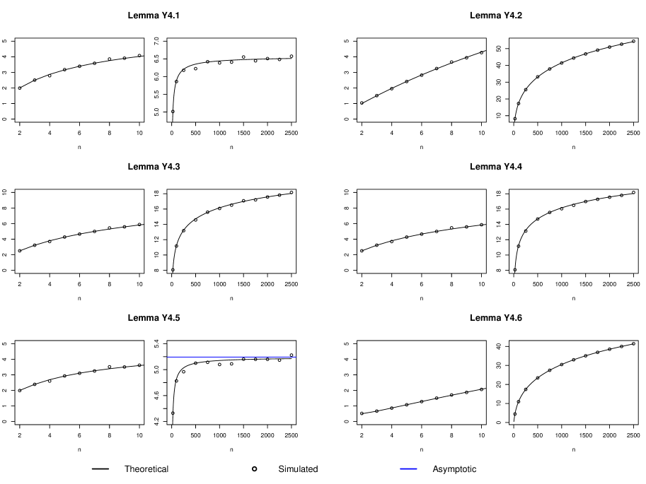
Figure 2: Comparison of simulated and theoretical values of Lemmata Y4.1 to Y4.6. For each lemma, the left-hand side plot shows values between 2 to 10, while the right-hand side plot shows values between 25 to 2500.

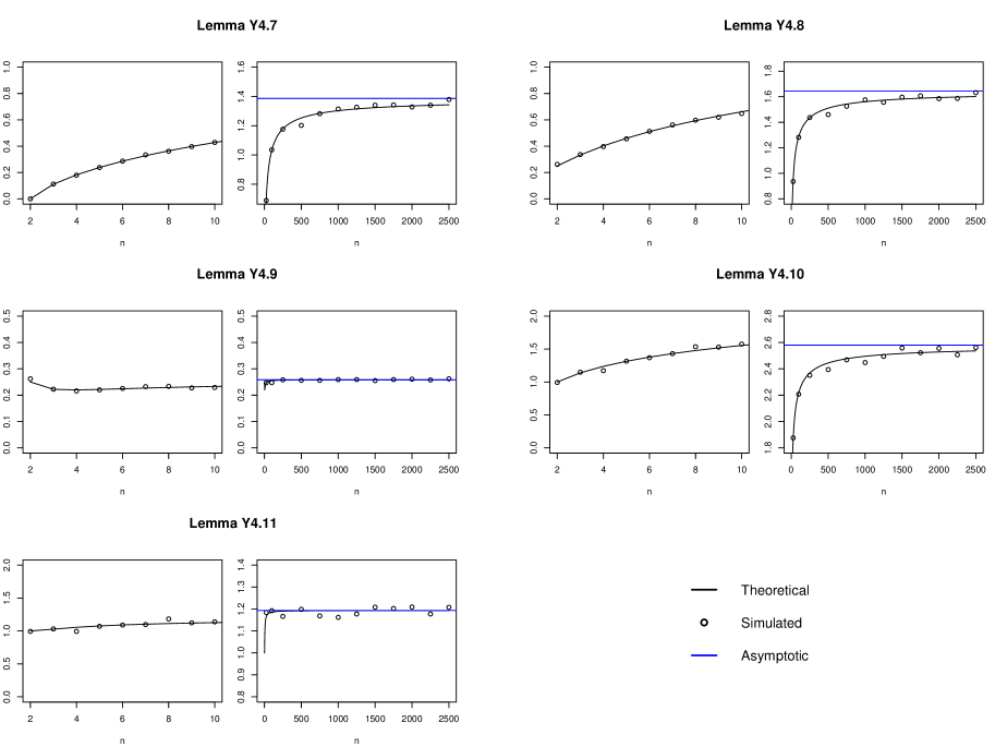
Figure 3: Comparison of simulated and theoretical values of Lemmata Y4.7 to Y4.11. For each lemma, the left-hand side plot shows values between 2 to 10, while the right-hand side plot shows values between 25 to 2500.

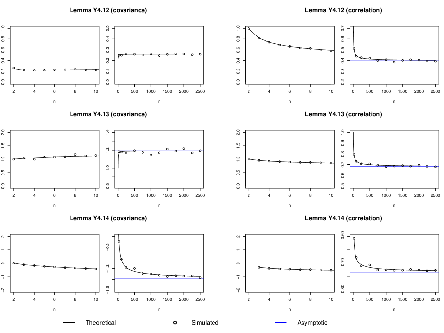
Figure 4: Comparison of simulated and theoretical values of Lemmata Y4.12 to Y4.14, where each lemma has a covariance and correlation part. For each lemma, the left-hand side plot shows values between 2 to 10, while the right-hand side plot shows values between 25 to 2500.

Algorithm Y5.1 Sampling $\operatorname{E}\left[\tau^{(n)}|\mathcal{Y}_{n}\right]$

1:Number of tips, $n$.

2:$\operatorname{E}\left[\tau^{(n)}|\mathcal{Y}_{n}\right]$

3:Generate a phylogenetic tree with $n$ number of tips, $\mathcal{Y}_{n}$, with internal nodes $z_{k}$, $k\in\{1,\cdots,n-1\}$, denoting the speciation points, and $T_{1},\cdots,T_{n}$ denoting the time intervals between speciation times.

4:for $k=1,\cdots,n-1$ do

5:  Compute $\text{ntips}(z_{k})$, number of tips of a subtree starting from $z_{k}$ (the $k$-th speciation event).

6:end for

7:for $k=1,\cdots,n-1$ do

8:  if $\text{ntips}(z_{k})>2$ then

9:   Set $l_{z_{k}}$, child node of $z_{k}$ on the left side.

10:   Set $r_{z_{k}}$, child node of $z_{k}$ on the right side.

11:   Compute $s_{k}:=\text{ntips}(l_{z_{k}})\times\text{ntips}(r_{z_{k}})$, number of possible pairs of tip nodes that coalesced at the $k$-th speciation event.

12:  else

13:   if $\text{ntips}(z_{k})==2$ then

14:     $s_{k}:=2$ ($z_{k}$ is a node above two tips)

15:   end if

16:  end if

17:end for

18:for $k=1,\cdots,n-1$ do

19:  Compute $\operatorname{E}\left[1_{k}^{(n)}|\mathcal{Y}_{n}\right]:=s_{k}/\sum_{j=1}^{n-1}s_{j}$

20:end forreturn $\operatorname{E}\left[\tau^{(n)}|\mathcal{Y}_{n}\right]=\sum_{k=1}^{n-1}\operatorname{E}\left[1_{k}^{(n)}|\mathcal{Y}_{n}\right]\sum_{j=k+1}^{n}T_{j}$

Code availability

In https://github.com/krzbar/YuleHeightMoments we provide code verifying our calculations. We checked the formulæ of Section Y4 numerically and where possible analytically with Mathematica. We further ran simulations in R, and in the repository random seeds, and output for Section Y5 can be found.

Appendix YA: Proofs of probabilities of coalescing at nodes from Bartoszek [2018]

In this section we provide proofs concerning coalescent events taking place at certain nodes. These formulæ  were obtained by Bartoszek [2018] with the help of Mathematica, here we present completely analytical derivations of them.

Lemma YA.1

We have that for $n>1$ and $1\leq k\leq n-1$

$$\begin{array}[]{l}\operatorname{E}\left[\operatorname{E}\left[1_{k}^{(n)}|\mathcal{Y}_{n}\right]^{2}\right]=\frac{16n(n+1)}{(n-1)^{2}(k+1)(k+2)(k+3)(k+4)}-\frac{16(n+1)}{(n-1)^{2}(k+1)(k+2)(k+3)}\\ +\frac{80(n+1)}{(n-1)^{2}(k+1)(k+2)(k+3)(k+4)}+\frac{4(n+1)}{(n-1)^{2}n(k+1)(k+2)}-\frac{32(n+1)}{(n-1)^{2}n(k+1)(k+2)(k+3)}\\ +\frac{96(n+1)}{(n-1)^{2}n(k+1)(k+2)(k+3)(k+4)}\end{array}$$

Proof We use the same approach as in KBar2018art Lemma $6.3$—considering the three possible ways that the two pairs could have been drawn, i.e., the same pair twice, they overlap with one tip, or are two disjoint pairs. For each of these three situations we have the expectation of the product of these indicator random variables (see below) multiplied by the probability of sampling such a pair. We remember that

$$\pi_{n,k}=\frac{2(n+1)}{n-1}\frac{1}{(k+1)(k+2)},$$

and then

$$\begin{array}[]{l}\operatorname{E}\left[1_{k,1}^{(n)}1_{k,2}^{(n)}\right]=\binom{n}{2}^{-1}\pi_{n,k}+2(n-2)\binom{n}{2}^{-1}4\frac{n+1}{(n-1)(n-2)}\frac{n-(k+1)}{(k+1)(k+2)(k+3)}\\ +\binom{n-2}{2}\binom{n}{2}^{-1}16\frac{n+1}{(n-1)(n-2)(n-3)}\frac{(n-(k+1))(n-(k+2))}{(k+1)(k+2)(k+3)(k+4)}\\ =\binom{n}{2}^{-1}\pi_{n,k}\left(1+4\frac{n-(k+1)}{k+3}+8\binom{n-2}{2}\frac{1}{(n-2)(n-3)}\frac{(n-(k+1))(n-(k+2))}{(k+3)(k+4)}\right)\\ =\frac{4(n+1)}{n(n-1)^{2}}\frac{1}{(k+1)(k+2)}\left(\frac{4n^{2}}{(k+3)(k+4)}-\frac{4n(k-1)}{(k+3)(k+4)}+\frac{k^{2}-k+4}{(k+3)(k+4)}\right)\\ =\frac{16n(n+1)}{(n-1)^{2}(k+1)(k+2)(k+3)(k+4)}-\frac{16(n+1)(k-1)}{(n-1)^{2}(k+1)(k+2)(k+3)(k+4)}+\frac{4(n+1)(k^{2}-k+4)}{(n-1)^{2}n(k+1)(k+2)(k+3)(k+4)}.\end{array}$$

We rewrite it in a form that will be useful later

$$\begin{array}[]{l}=\frac{16n(n+1)}{(n-1)^{2}(k+1)(k+2)(k+3)(k+4)}-\frac{16(n+1)}{(n-1)^{2}(k+1)(k+2)(k+3)}+\frac{80(n+1)}{(n-1)^{2}(k+1)(k+2)(k+3)(k+4)}\\ +\frac{4(n+1)}{(n-1)^{2}n(k+1)(k+2)}-\frac{32(n+1)}{(n-1)^{2}n(k+1)(k+2)(k+3)}+\frac{96(n+1)}{(n-1)^{2}n(k+1)(k+2)(k+3)(k+4)}.\end{array}$$

For completeness it remains to fill in the parts of KBar2018art proof of the therein Lemma $6.3$ that Mathematica was used for—$\operatorname{E}\left[1_{k,1}^{(n)}1_{k,2}^{(n)}\right]$ conditional on how the two random pairs were sampled, i.e., whether they are distinct or have a tip in common (see KBar2018art Fig. $4$). We show that when they have a tip in common then the conditional expectation of the above product is

$$\begin{array}[]{l}\sum\limits_{j=k+1}^{n-1}\left(1-\frac{3}{\binom{n}{2}}\right)\cdots\left(1-\frac{3}{\binom{j+2}{2}}\right)\frac{1}{\binom{j+1}{2}}\left(1-\frac{1}{\binom{j}{2}}\right)\cdots\left(1-\frac{1}{\binom{k+2}{2}}\right)\frac{1}{\binom{k+1}{2}}\\ =\sum\limits_{j=k+1}^{n-1}\left(\frac{(n+2)(n-3)}{n(n-1)}\cdots\frac{(j+4)(j-1)}{(j+2)(j-1)}\frac{2}{j(j+1)}\frac{(j+1)(j-2)}{j(j-1)}\cdots\frac{(k+3)k}{(k+2)(k+1)}\frac{2}{k(k+1)}\right)\\ =\sum\limits_{j=k+1}^{n-1}\left(\frac{(n+2)!(n-3)!}{n!(n-1)!}\frac{(j+1)!j!}{(j+3)!(j-2)!}\frac{2}{j(j+1)}\frac{(j+1)!(j-2)!}{j!(j-1)!}\frac{(k+1)!k!}{(k+2)!(k-1)!}\frac{2}{k(k+1)}\right)\\ =\sum\limits_{j=k+1}^{n-1}\left(\frac{(n+2)(n+1)}{(n-1)(n-2)}\frac{(j-1)j}{(j+2)(j+3)}\frac{2}{j(j+1)}\frac{(j+1)}{j}\frac{k}{(k+2)}\frac{2}{k(k+1)}\right)\end{array}$$

$$\begin{array}[]{l}\\ =4\frac{(n+2)(n+1)}{(n-1)(n-2)}\frac{1}{(k+1)(k+2)}\sum\limits_{j=k+1}^{n-1}\frac{1}{(j+2)(j+3)}\stackrel{{\scriptstyle Lemma~\ref{HarXiv-lemSumj2j3}}}{{=}}4\frac{(n+2)(n+1)}{(n-1)(n-2)}\frac{1}{(k+1)(k+2)}\left(\frac{1}{3}-\frac{1}{n+2}\right)\\ =\frac{4(n+1)}{(n-1)(n-2)}\frac{(n-(k+1))}{(k+1)(k+2)(k+3)},\end{array}$$

and when the two pairs are distinct this conditional expectation becomes

$$\begin{array}[]{l}\sum\limits_{j_{2}=k+2}^{n-1}\sum\limits_{j_{1}=k+1}^{j_{2}-1}\left(1-\frac{6}{\binom{n}{2}}\right)\cdots\left(1-\frac{6}{\binom{j_{2}+2}{2}}\right)\frac{4}{\binom{j_{2}+1}{2}}\left(1-\frac{3}{\binom{j_{2}}{2}}\right)\cdots\left(1-\frac{3}{\binom{j_{1}+2}{2}}\right)\frac{1}{\binom{j_{1}+1}{2}}\\ \cdot\left(1-\frac{1}{\binom{j_{1}}{2}}\right)\cdots\left(1-\frac{1}{\binom{k+2}{2}}\right)\frac{1}{\binom{k+1}{2}}\\ =\sum\limits_{j_{2}=k+2}^{n-1}\sum\limits_{j_{1}=k+1}^{j_{2}-1}\left(\frac{(n+3)(n-4)}{n(n-1)}\cdots\frac{(j_{2}+5)(j_{2}-2)}{(j_{2}+2)(j_{2}+1)}\frac{8}{j_{2}(j_{2}+1)}\frac{(j_{2}+2)(j_{2}+1)}{(j_{2}-1)(j_{2}-2)}\frac{(j_{1}-1)j_{1}}{(j_{1}+2)(j_{1}+3)}\frac{2}{j_{1}(j_{1}+1)}\frac{j_{1}+1}{j_{1}-1}\frac{k}{k+2}\frac{2}{k(k+1)}\right)\\ =\frac{32(n+3)(n+2)(n+1)}{(n-1)(n-2)(n-3)(k+2)(k+1)}\sum\limits_{j_{2}=k+2}^{n-1}\frac{1}{(j_{2}+3)(j_{2}+4)}\sum\limits_{j_{1}=k+1}^{j_{2}-1}\frac{1}{(j_{1}+2)(j_{1}+3)}\\ \stackrel{{\scriptstyle Lemma~\ref{HarXiv-lemSumj2j3}}}{{=}}\frac{32(n+3)(n+2)(n+1)}{(n-1)(n-2)(n-3)(k+2)(k+1)}\left(\frac{1}{(k+3)}\sum\limits_{j_{2}=k+2}^{n-1}\frac{1}{(j_{2}+3)(j_{2}+4)}-\sum\limits_{j_{2}=k+2}^{n-1}\frac{1}{(j_{2}+2)(j_{2}+3)(j_{2}+4)}\right)\\ \stackrel{{\scriptstyle Lemma~\ref{HarXiv-lemSumj3j4},\ref{HarXiv-lemSumj2j3j4}}}{{=}}\\ \frac{32(n+3)(n+2)(n+1)}{(n-1)(n-2)(n-3)(k+2)(k+1)}\left(\frac{1}{(k+3)(k+5)}-\frac{1}{(k+3)(n+3)}-\frac{1}{2(k+4)}+\frac{1}{2(k+5)}+\frac{1}{2(n+2)}-\frac{1}{2(n+3)}\right)\\ =\frac{16(n+1)}{(n-1)(n-2)(n-3)}\frac{(n-(k+1))(n-(k+2))}{(k+1)(k+2)(k+3)(k+4)}.\end{array}$$

We can also recover $\operatorname{Var}\left[\operatorname{E}\left[1_{k}^{(n)}|\mathcal{Y}_{n}\right]\right]$ (KBar2018art Lemma $6.3$)

$$\begin{array}[]{l}\operatorname{Var}\left[\operatorname{E}\left[1_{k}^{(n)}|\mathcal{Y}_{n}\right]\right]=\operatorname{E}\left[\operatorname{E}\left[1_{k}^{(n)}|\mathcal{Y}_{n}\right]^{2}\right]-\pi_{n,k}^{2}\\ =\frac{16n(n+1)}{(n-1)^{2}(k+1)(k+2)(k+3)(k+4)}-\frac{16(n+1)(k-1)}{(n-1)^{2}(k+1)(k+2)(k+3)(k+4)}+\frac{4(n+1)(k^{2}-k+4)}{(n-1)^{2}n(k+1)(k+2)(k+3)(k+4)}\\ -\left(2\frac{n+1}{n-1}\frac{1}{(k+1)(k+2)}\right)^{2}\\ =4\frac{n+1}{n(n-1)^{2}}\frac{(n-(k+1))(n(3k^{2}+5k-4)-(k^{3}+k^{2}+2k+8))}{(k+1)^{2}(k+2)^{2}(k+3)(k+4)}.\end{array}$$

$\Box$

Lemma YA.2

For $1\leq k_{1}<k_{2}\leq n-1$ it holds that

$$\begin{array}[]{l}\operatorname{E}\left[\operatorname{E}\left[1_{k_{2}}^{(n)}|\mathcal{Y}_{n}\right]\operatorname{E}\left[1_{k_{1}}^{(n)}|\mathcal{Y}_{n}\right]\right]=\frac{4(n+1)^{2}}{(n-1)^{2}(k_{1}+1)(k_{1}+2)(k_{2}+1)(k_{2}+2)}\\ -\frac{24n(n+1)}{(n-1)^{2}(k_{1}+1)(k_{1}+2)(k_{2}+1)(k_{2}+2)(k_{2}+3)(k_{2}+4)}+\frac{32(n+1)}{(n-1)^{2}(k_{1}+1)(k_{1}+2)(k_{2}+1)(k_{2}+2)(k_{2}+3)}\\ -\frac{120(n+1)}{(n-1)^{2}(k_{1}+1)(k_{1}+2)(k_{2}+1)(k_{2}+2)(k_{2}+3)(k_{2}+4)}-\frac{8(n+1)}{(n-1)^{2}n(k_{1}+1)(k_{1}+2)(k_{2}+1)(k_{2}+2)}\\ +\frac{64(n+1)}{(n-1)^{2}n(k_{1}+1)(k_{1}+2)(k_{2}+1)(k_{2}+2)(k_{2}+3)}-\frac{144(n+1)}{(n-1)^{2}n(k_{1}+1)(k_{1}+2)(k_{2}+1)(k_{2}+2)(k_{2}+3)(k_{2}+4)}.\end{array}$$ (YA.1)

Proof From KBar2018art Lemma $6.4$ we obtain

$$\begin{array}[]{l}\operatorname{E}\left[\operatorname{E}\left[1_{k_{2}}^{(n)}|\mathcal{Y}_{n}\right]\operatorname{E}\left[1_{k_{1}}^{(n)}|\mathcal{Y}_{n}\right]\right]=\operatorname{Cov}\left[\operatorname{E}\left[1_{k_{2}}^{(n)}|\mathcal{Y}_{n}\right],\operatorname{E}\left[1_{k_{1}}^{(n)}|\mathcal{Y}_{n}\right]\right]+\pi_{n,k_{1}}\pi_{n,k_{2}}\\ =\frac{-8(n+1)(3n-(k_{2}-2))(n-(k_{2}+1))}{n(n-1)^{2}(k_{1}+1)(k_{1}+2)(k_{2}+1)(k_{2}+2)(k_{2}+3)(k_{2}+4)}+4\frac{(n+1)^{2}}{(n-1)^{2}}\frac{1}{(k_{1}+1)(k_{1}+2)(k_{2}+1)(k_{2}+2)}\\ =\frac{4(n+1)^{2}}{(n-1)^{2}}\frac{1}{(k_{1}+1)(k_{1}+2)(k_{2}+1)(k_{2}+2)}-\frac{24n(n+1)}{(n-1)^{2}}\frac{1}{(k_{1}+1)(k_{1}+2)(k_{2}+1)(k_{2}+2)(k_{2}+3)(k_{2}+4)}\\ +\frac{24(n+1)}{(n-1)^{2}}\frac{1}{(k_{1}+1)(k_{1}+2)(k_{2}+1)(k_{2}+2)(k_{2}+3)}-\frac{120(n+1)}{(n-1)^{2}}\frac{1}{(k_{1}+1)(k_{1}+2)(k_{2}+1)(k_{2}+2)(k_{2}+3)(k_{2}+4)}\\ +\frac{8(n+1)}{(n-1)^{2}}\frac{1}{(k_{1}+1)(k_{1}+2)(k_{2}+1)(k_{2}+2)(k_{2}+3)}-\frac{8(n+1)}{n(n-1)^{2}}\frac{1}{(k_{1}+1)(k_{1}+2)(k_{2}+1)(k_{2}+2)}\\ +\frac{64(n+1)}{n(n-1)^{2}}\frac{1}{(k_{1}+1)(k_{1}+2)(k_{2}+1)(k_{2}+2)(k_{2}+3)}-\frac{144(n+1)}{n(n-1)^{2}}\frac{1}{(k_{1}+1)(k_{1}+2)(k_{2}+1)(k_{2}+2)(k_{2}+3)(k_{2}+4)}.\end{array}$$

For completeness it remains to fill in the parts of KBar2018art proof of the therein Lemma $6.4$ that Mathematica was used for—the value of the expectation of this product of indicator random variables, depending on how the two pairs of tips were sampled and how their coalescence pattern looks like (see KBar2018art Fig. $5$). We show that when the two pairs have a tip in common,

$$\begin{array}[]{l}\left(1-\frac{3}{\binom{n}{2}}\right)\cdots\left(1-\frac{3}{\binom{k_{2}+2}{2}}\right)\frac{1}{\binom{k_{2}+1}{2}}\left(1-\frac{1}{\binom{k_{2}}{2}}\right)\cdots\left(1-\frac{1}{\binom{k_{1}+2}{2}}\right)\frac{1}{\binom{k_{1}+1}{2}}\\ =\frac{(n+2)(n-3)}{n(n-1)}\cdots\frac{(k_{2}+4)(k_{2}-1)}{(k_{2}+2)(k_{2}-1)}\frac{2}{k_{2}(k_{2}+1)}\frac{(k_{2}+1)(k_{2}-2)}{k_{2}(k_{2}-1)}\cdots\frac{(k_{1}+3)k}{(k_{1}+2)(k_{1}+1)}\frac{2}{k_{1}(k_{1}+1)}\\ =\frac{4(n+1)(n+2)}{(n-1)(n-2)}\frac{1}{(k_{1}+1)(k_{1}+2)(k_{2}+2)(k_{2}+3)},\end{array}$$

and when they are two disjoint pairs

$$\begin{array}[]{l}\left(1-\frac{6}{\binom{n}{2}}\right)\cdots\left(1-\frac{6}{\binom{k_{2}+2}{2}}\right)\frac{1}{\binom{k_{2}+1}{2}}\left(1-\frac{3}{\binom{k_{2}}{2}}\right)\cdots\left(1-\frac{3}{\binom{k_{1}+2}{2}}\right)\frac{1}{\binom{k_{1}+1}{2}}\\ +\sum\limits_{j=k_{1}+1}^{k_{2}-1}\left(1-\frac{6}{\binom{n}{2}}\right)\cdots\left(1-\frac{6}{\binom{k_{2}+2}{2}}\right)\frac{1}{\binom{k_{2}+1}{2}}\left(1-\frac{3}{\binom{k_{2}}{2}}\right)\cdots\left(1-\frac{3}{\binom{j+2}{2}}\right)\frac{2}{\binom{j+1}{2}}\\ \cdot\left(1-\frac{1}{\binom{j}{2}}\right)\cdots\left(1-\frac{1}{\binom{k_{1}+2}{2}}\right)\frac{1}{\binom{k_{1}+1}{2}}\\ +\sum\limits_{j=k_{2}+1}^{n-1}\left(1-\frac{6}{\binom{n}{2}}\right)\cdots\left(1-\frac{6}{\binom{j+2}{2}}\right)\frac{4}{\binom{j+1}{2}}\left(1-\frac{3}{\binom{j}{2}}\right)\cdots\left(1-\frac{3}{\binom{k_{2}+2}{2}}\right)\frac{1}{\binom{k_{2}+1}{2}}\\ \cdot\left(1-\frac{1}{\binom{k_{2}}{2}}\right)\cdots\left(1-\frac{1}{\binom{k_{1}+2}{2}}\right)\frac{1}{\binom{k_{1}+1}{2}}\end{array}$$

$$\begin{array}[]{l}=\frac{(n+3)(n+2)(n+1)}{(n-1)(n-2)(n-3)}\frac{k_{2}(k_{2}-1)(k_{2}-2)}{(k_{2}+4)(k_{2}+3)(k_{2}+2)}\frac{2}{k_{2}(k_{2}+1)}\frac{(k_{2}+2)(k_{2}+1)}{(k_{2}-1)(k_{2}-2)}\frac{(k_{1}-1)k_{1}}{(k_{1}+2)(k_{1}+3)}\frac{2}{k_{1}(k_{1}+1)}\\ +\sum\limits_{j=k_{1}+1}^{k_{2}-1}\frac{(n+3)(n+2)(n+1)}{(n-1)(n-2)(n-3)}\frac{k_{2}(k_{2}-1)(k_{2}-2)}{(k_{2}+4)(k_{2}+3)(k_{2}+2)}\frac{2}{k_{2}(k_{2}+1)}\frac{(k_{2}+2)(k_{2}+1)}{(k_{2}-1)(k_{2}-2)}\frac{(j-1)j}{(j+2)(j+3)}\frac{4}{j(j+1)}\frac{(j+1)}{(j-1)}\frac{k_{1}}{k_{1}+2}\frac{2}{k_{1}(k_{1}+1)}\\ +\sum\limits_{j=k_{2}+1}^{n-1}\frac{(n+3)(n+2)(n+1)}{(n-1)(n-2)(n-3)}\frac{j(j-1)(j-2)}{(j+4)(j+3)(j+2)}\frac{8}{j(j+1)}\frac{(j+2)(j+1)}{(j-1)(j-2)}\frac{(k_{2}-1)k_{2}}{(k_{2}+2)(k_{2}+3)}\frac{2}{k_{2}(k_{2}+1)}\frac{(k_{2}+1)}{(k_{2}-1)}\frac{k_{1}}{k_{1}+2}\frac{2}{k_{1}(k_{1}+1)}\\ =\frac{4(n+3)(n+2)(n+1)}{(n-1)(n-2)(n-3)}\frac{1}{(k_{2}+3)(k_{2}+4)}\frac{(k_{1}-1)}{(k_{1}+1)(k_{1}+2)(k_{1}+3)}\\ +\frac{16(n+3)(n+2)(n+1)}{(n-1)(n-2)(n-3)}\frac{1}{(k_{2}+3)(k_{2}+4)}\frac{1}{(k_{1}+1)(k_{1}+2)}\sum\limits_{j=k_{1}+1}^{k_{2}-1}\frac{1}{(j+2)(j+3)}\\ +\frac{32(n+3)(n+2)(n+1)}{(n-1)(n-2)(n-3)}\frac{1}{(k_{2}+2)(k_{2}+3)}\frac{1}{(k_{1}+1)(k_{1}+2)}\sum\limits_{j=k_{2}+1}^{n-1}\frac{1}{(j+3)(j+4)}\end{array}$$

$$\begin{array}[]{l}\stackrel{{\scriptstyle Lemmata~\ref{HarXiv-lemSumj2j3},\ref{HarXiv-lemSumj3j4}}}{{=}}\\ \frac{4(n+3)(n+2)(n+1)}{(n-1)(n-2)(n-3)}\frac{1}{(k_{2}+3)(k_{2}+4)}\frac{(k_{1}-1)}{(k_{1}+1)(k_{1}+2)(k_{1}+3)}\\ +\frac{16(n+3)(n+2)(n+1)}{(n-1)(n-2)(n-3)}\frac{1}{(k_{2}+3)(k_{2}+4)}\frac{1}{(k_{1}+1)(k_{1}+2)}\left(\frac{1}{k_{1}+3}-\frac{1}{k_{2}+2}\right)\\ +\frac{32(n+3)(n+2)(n+1)}{(n-1)(n-2)(n-3)}\frac{1}{(k_{2}+2)(k_{2}+3)}\frac{1}{(k_{1}+1)(k_{1}+2)}\left(\frac{1}{k_{2}+4}-\frac{1}{n+3}\right)\\ =\frac{4(n+1)(n+2)}{(n-1)(n-2)(n-3)}\frac{n(k_{2}+6)-5k_{2}-14}{(k_{1}+1)(k_{1}+2)(k_{2}+2)(k_{2}+3)(k_{2}+4)}.\end{array}$$

$\Box$

Appendix YB: Direct, alternative proofs of Lemmata Y4.1 and Y4.5

Lemma Y4.1 For a Yule tree with speciation rate $\lambda=1$ we have

$$\operatorname{E}\left[(U^{(n)}-\tau^{(n)})^{2}\right]=\frac{4n+2}{n-1}H_{n,2}-\frac{2H_{n,1}^{2}}{n-1}-\frac{4H_{n,1}}{n-1}$$

Proof We derived Lemma Y4.1 from a joint moments formula but the same result can be obtained directly. By Lemmata LABEL:HarXiv-lemSumHii1, LABEL:HarXiv-lemSumHi2i1i2, and LABEL:HarXiv-lemSumHisqi1i2app we have

$$\begin{array}[]{l}\operatorname{E}\left[(U^{(n)}-\tau^{(n)})^{2}\right]=\sum\limits_{k=1}^{n-1}\pi_{n,k}\operatorname{E}\left[(U^{(n)}-\tau^{(n)})^{2}|\kappa_{n}=k\right]=\sum\limits_{k=1}^{n-1}\pi_{n,k}\operatorname{E}\left[\left(\sum\limits_{i=1}^{k}T_{k}\right)^{2}\right]\\ =\sum\limits_{k=1}^{n-1}\pi_{n,k}\left(\sum\limits_{i=1}^{k}\operatorname{E}\left[T_{i}^{2}\right]+2\sum\limits_{i_{2}<i_{1}}^{k}\operatorname{E}\left[T_{i_{1}}T_{i_{2}}\right]\right)=\frac{2(n+1)}{n-1}\sum\limits_{k=1}^{n-1}\frac{1}{(k+1)(k+2)}\left(\sum\limits_{i=1}^{k}\frac{2}{i^{2}}+2\sum\limits_{i_{2}<i_{1}}^{k}\frac{1}{i_{1}}\frac{1}{i_{2}}\right)\\ =\frac{2(n+1)}{n-1}\left(\sum\limits_{k=1}^{n-1}\frac{2H_{k,2}}{(k+1)(k+2)}+2\sum\limits_{k=1}^{n-1}\frac{1}{(k+1)(k+2)}\left(\sum\limits_{i_{1}=1}^{k}\frac{H_{i_{1},1}}{i_{1}}-1-\sum\limits_{i_{1}=1}^{k}\frac{1}{i_{1}^{2}}+1\right)\right)\\ \stackrel{{\scriptstyle\mathrm{Lemma~}\ref{HarXiv-lemSumHii1}}}{{=}}\frac{2(n+1)}{n-1}\left(\sum\limits_{k=1}^{n-1}\frac{2H_{k,2}}{(k+1)(k+2)}+2\sum\limits_{k=1}^{n-1}\frac{1}{(k+1)(k+2)}\left(\frac{1}{2}(H_{k,1}^{2}+H_{k,2})-H_{k,2}\right)\right)\\ =\frac{2(n+1)}{n-1}\left(\sum\limits_{k=1}^{n-1}\frac{H_{k,2}}{(k+1)(k+2)}+\sum\limits_{k=1}^{n-1}\frac{H_{k,1}^{2}}{(k+1)(k+2)}\right)\\ \stackrel{{\scriptstyle\mathrm{Lemmata~}\ref{HarXiv-lemSumHi2i1i2},~\ref{HarXiv-lemSumHisqi1i2app}}}{{=}}\frac{2(n+1)}{n-1}\left(\frac{n}{n+1}\left(H_{n,2}-1\right)+H_{n,2}+\frac{(n-1)^{2}+n-1-1}{n^{2}}-2\frac{H_{n-1,1}}{n}-\frac{H_{n-1,1}^{2}}{n+1}\right)\\ =\frac{4n+2}{n-1}H_{n,2}-\frac{2H_{n,1}^{2}}{n-1}-\frac{4H_{n,1}}{n-1}.\end{array}$$

We can see that we obtain the same formula as in Eq. (Y4.8).

$\Box$

Lemma Y4.5 For a Yule tree with speciation rate $\lambda=1$ we have

$$\begin{array}[]{l}\operatorname{E}\left[(U^{(n)}-\operatorname{E}\left[\tau^{(n)}|\mathcal{Y}_{n}\right])^{2}\right]=\frac{4}{3}H_{n,2}+3-8n^{-1}H_{n,1}+\Theta(n^{-1})\xrightarrow{n\to\infty}\frac{2\pi^{2}}{9}+3.\end{array}$$

Proof We present here an alternative, direct, proof of Lemma Y4.5 based on the same techniques that were used to show Lemmata $11$ [Bartoszek and Sagitov, 2015a] and $5.1$, $5.3$, $5.5$ [Bartoszek, 2020]. Denote by $\tau^{(n)}_{1}$ and $\tau^{(n)}_{2}$ two versions of $\tau^{(n)}$ that are independent given $\mathcal{Y}_{n}$. This allows us to write

$$\begin{array}[]{l}\operatorname{E}\left[(U^{(n)}-\operatorname{E}\left[\tau^{(n)}|\mathcal{Y}_{n}\right])^{2}\right]=\operatorname{E}\left[(\operatorname{E}\left[U^{(n)}-\tau^{(n)}|\mathcal{Y}_{n}\right])^{2}\right]=\operatorname{E}\left[(U^{(n)}-\tau^{(n)}_{1})(U^{(n)}-\tau^{(n)}_{2})\right]\\ =\sum\limits_{k=1}^{n-1}\operatorname{E}\left[\left(\sum\limits_{i=1}^{k}T_{i}\right)^{2}\right]\operatorname{E}\left[\operatorname{E}\left[1_{k}^{(n)}|\mathcal{Y}_{n}\right]^{2}\right]+2\sum\limits_{k_{1}=1}^{n-1}\sum\limits_{k_{2}=k_{1}+1}^{n-1}\operatorname{E}\left[\left(\sum\limits_{i_{1}=1}^{k_{1}}T_{i_{1}}\right)\left(\sum\limits_{i_{2}=1}^{k_{2}}T_{i_{2}}\right)\right]\operatorname{E}\left[1_{k,1}^{(n)}1_{k,2}^{(n)}\right]\end{array}$$

$$\begin{array}[]{l}=\sum\limits_{k=1}^{n-1}\operatorname{E}\left[\left(\sum\limits_{i=1}^{k}T_{i}\right)^{2}\right]\operatorname{E}\left[\operatorname{E}\left[1_{k}^{(n)}|\mathcal{Y}_{n}\right]^{2}\right]\\ +2\left(\sum\limits_{k_{1}=1}^{n-1}\sum\limits_{k_{2}=k_{1}+1}^{n-1}\operatorname{E}\left[\left(\sum\limits_{i_{1}=1}^{k_{1}}T_{i_{1}}\right)\left(\sum\limits_{i_{2}=1}^{k_{1}}T_{i_{2}}+\sum\limits_{i_{2}=k_{1}+1}^{k_{2}}T_{i_{2}}\right)\right]\operatorname{E}\left[1_{k,1}^{(n)}1_{k,2}^{(n)}\right]\right)\\ =\sum\limits_{k=1}^{n-1}\operatorname{E}\left[\left(\sum\limits_{i=1}^{k}T_{i}\right)^{2}\right]\operatorname{E}\left[\operatorname{E}\left[1_{k}^{(n)}|\mathcal{Y}_{n}\right]^{2}\right]\\ +2\left(\sum\limits_{k_{1}=1}^{n-1}\sum\limits_{k_{2}=k_{1}+1}^{n-1}\left(\operatorname{E}\left[\left(\sum\limits_{i_{1}=1}^{k_{1}}T_{i_{1}}\right)^{2}\right]+\operatorname{E}\left[\left(\sum\limits_{i_{1}=1}^{k_{1}}T_{i_{1}}\right)\right]\operatorname{E}\left[\left(\sum\limits_{i_{2}=k_{1}+1}^{k_{2}}T_{i_{2}}\right)\right]\right)\operatorname{E}\left[1_{k,1}^{(n)}1_{k,2}^{(n)}\right]\right).\end{array}$$

Using that $T_{i}$ is exponentially distributed with rate $i$, we calculate

$$\begin{array}[]{l}E{\left(\sum\limits_{i=1}^{k}T_{i}\right)^{2}}=\operatorname{E}\left[\sum\limits_{i=1}^{k}T_{i}^{2}+2\sum\limits_{i_{1}=1}^{k}\sum\limits_{i_{2}=i_{1}+1}^{k}T_{i_{1}}T_{i_{2}}\right]\\ =\sum\limits_{i=1}^{k}\operatorname{E}\left[T_{i}^{2}\right]+2\sum\limits_{i_{1}=1}^{k}\sum\limits_{i_{2}=i_{1}+1}^{k}\operatorname{E}\left[T_{i_{1}}\right]\operatorname{E}\left[T_{i_{2}}\right]=2H_{k,2}+2\sum\limits_{i_{1}=1}^{k}\frac{1}{i_{1}}\left(H_{k,1}-H_{i_{1},1}\right)\\ =2H_{k,2}+2H_{k,1}^{2}-2\sum\limits_{i_{1}=1}^{k}\frac{H_{i_{1},1}}{i_{1}}\stackrel{{\scriptstyle Lemma~\ref{HarXiv-lemSumHii1}}}{{=}}2H_{k,2}+2H_{k,1}^{2}-\left(H_{k,1}^{2}+H_{k,2}\right)=H_{k,2}+H_{k,1}^{2}.\end{array}$$

We continue with plugging the above calculation back into our main derivations

$$\begin{array}[]{l}\operatorname{E}\left[(U^{(n)}-\operatorname{E}\left[\tau^{(n)}|\mathcal{Y}_{n}\right])^{2}\right]=\sum\limits_{k=1}^{n-1}\left(H_{k,2}+H_{k,1}^{2}\right)\operatorname{E}\left[\operatorname{E}\left[1_{k}^{(n)}|\mathcal{Y}_{n}\right]^{2}\right]\\ +2\left(\sum\limits_{k_{1}=1}^{n-1}\sum\limits_{k_{2}=k_{1}+1}^{n-1}\left(\left(H_{k_{1},2}+H_{k_{1},1}^{2}\right)+H_{k_{1},1}\left(H_{k_{2},1}-H_{k_{1},1}\right)\right)\operatorname{E}\left[1_{k,1}^{(n)}1_{k,2}^{(n)}\right]\right)\\ =\sum\limits_{k=1}^{n-1}\left(H_{k,2}+H_{k,1}^{2}\right)\operatorname{E}\left[\operatorname{E}\left[1_{k}^{(n)}|\mathcal{Y}_{n}\right]^{2}\right]\\ +2\left(\sum\limits_{k_{1}=1}^{n-1}\sum\limits_{k_{2}=k_{1}+1}^{n-1}\left(H_{k_{1},2}+H_{k_{1},1}^{2}+H_{k_{1},1}H_{k_{2},1}-H_{k_{1},1}^{2}\right)\operatorname{E}\left[1_{k,1}^{(n)}1_{k,2}^{(n)}\right]\right)\end{array}$$

$$\begin{array}[]{l}=\sum\limits_{k=1}^{n-1}\left(H_{k,2}+H_{k,1}^{2}\right)\left(\frac{16n(n+1)}{(n-1)^{2}(k+1)(k+2)(k+3)(k+4)}-\frac{16(n+1)}{(n-1)^{2}(k+1)(k+2)(k+3)}\right.\\ \left.+\frac{80(n+1)}{(n-1)^{2}(k+1)(k+2)(k+3)(k+4)}+\frac{4(n+1)}{(n-1)^{2}n(k+1)(k+2)}-\frac{32(n+1)}{(n-1)^{2}n(k+1)(k+2)(k+3)}\right.\\ \left.+\frac{96(n+1)}{(n-1)^{2}n(k+1)(k+2)(k+3)(k+4)}\right)\\ +2\left(\sum\limits_{k_{1}=1}^{n-1}\sum\limits_{k_{2}=k_{1}+1}^{n-1}\left(H_{k_{1},2}+H_{k_{1},1}H_{k_{2},1}\right)\left(\frac{4(n+1)^{2}}{(n-1)^{2}(k_{1}+1)(k_{1}+2)(k_{2}+1)(k_{2}+2)}\right.\right.\\ \left.\left.-\frac{24n(n+1)}{(n-1)^{2}(k_{1}+1)(k_{1}+2)(k_{2}+1)(k_{2}+2)(k_{2}+3)(k_{2}+4)}+\frac{32(n+1)}{(n-1)^{2}(k_{1}+1)(k_{1}+2)(k_{2}+1)(k_{2}+2)(k_{2}+3)}\right.\right.\\ \left.\left.-\frac{120(n+1)}{(n-1)^{2}(k_{1}+1)(k_{1}+2)(k_{2}+1)(k_{2}+2)(k_{2}+3)(k_{2}+4)}-\frac{8(n+1)}{(n-1)^{2}n(k_{1}+1)(k_{1}+2)(k_{2}+1)(k_{2}+2)}\right.\right.\\ \left.\left.+\frac{64(n+1)}{(n-1)^{2}n(k_{1}+1)(k_{1}+2)(k_{2}+1)(k_{2}+2)(k_{2}+3)}-\frac{144(n+1)}{(n-1)^{2}n(k_{1}+1)(k_{1}+2)(k_{2}+1)(k_{2}+2)(k_{2}+3)(k_{2}+4)}\right)\right)\end{array}$$

$$\begin{array}[]{l}=\left(\frac{16n(n+1)}{(n-1)^{2}}+\frac{80(n+1)}{(n-1)^{2}}+\frac{96(n+1)}{(n-1)^{2}n}\right)\sum\limits_{k=1}^{n-1}\frac{H_{k,2}+H_{k,1}^{2}}{(k+1)(k+2)(k+3)(k+4)}\\ -\left(\frac{16(n+1)}{(n-1)^{2}}+\frac{32(n+1)}{(n-1)^{2}n}\right)\sum\limits_{k=1}^{n-1}\frac{H_{k,2}+H_{k,1}^{2}}{(k+1)(k+2)(k+3)}+\frac{4(n+1)}{(n-1)^{2}n}\sum\limits_{k=1}^{n-1}\frac{H_{k,2}+H_{k,1}^{2}}{(k+1)(k+2)}\\ +2\sum\limits_{k_{1}=1}^{n-1}\frac{H_{k_{1},2}}{(k_{1}+1)(k_{1}+2)}\left(\left(\frac{4(n+1)^{2}}{(n-1)^{2}}-\frac{8(n+1)}{(n-1)^{2}n}\right)\sum\limits_{k_{2}=k_{1}+1}^{n-1}\frac{1}{(k_{2}+1)(k_{2}+2)}\right.\\ \left.+\left(\frac{32(n+1)}{(n-1)^{2}}+\frac{64(n+1)}{(n-1)^{2}n}\right)\sum\limits_{k_{2}=k_{1}+1}^{n-1}\frac{1}{(k_{2}+1)(k_{2}+2)(k_{2}+3)}\right.\\ \left.-\left(\frac{24n(n+1)}{(n-1)^{2}}+\frac{120(n+1)}{(n-1)^{2}}+\frac{144(n+1)}{(n-1)^{2}n}\right)\sum\limits_{k_{2}=k_{1}+1}^{n-1}\frac{1}{(k_{2}+1)(k_{2}+2)(k_{2}+3)(k_{2}+4)}\right)\\ +2\sum\limits_{k_{1}=1}^{n-1}\frac{H_{k_{1},1}}{(k_{1}+1)(k_{1}+2)}\left(\left(\frac{4(n+1)^{2}}{(n-1)^{2}}-\frac{8(n+1)}{(n-1)^{2}n}\right)\sum\limits_{k_{2}=k_{1}+1}^{n-1}\frac{H_{k_{2},1}}{(k_{2}+1)(k_{2}+2)}\right.\\ \left.+\left(\frac{32(n+1)}{(n-1)^{2}}+\frac{64(n+1)}{(n-1)^{2}n}\right)\sum\limits_{k_{2}=k_{1}+1}^{n-1}\frac{H_{k_{2},1}}{(k_{2}+1)(k_{2}+2)(k_{2}+3)}\right.\\ \left.-\left(\frac{24n(n+1)}{(n-1)^{2}}+\frac{120(n+1)}{(n-1)^{2}}+\frac{144(n+1)}{(n-1)^{2}n}\right)\sum\limits_{k_{2}=k_{1}+1}^{n-1}\frac{H_{k_{2},1}}{(k_{2}+1)(k_{2}+2)(k_{2}+3)(k_{2}+4)}\right)\end{array}$$

$$\begin{array}[]{l}\stackrel{{\scriptstyle Lemmata~\ref{HarXiv-lemSum1},\ref{HarXiv-lemSumj1j2j3},\ref{HarXiv-lemSumj1j2j3j4},\ref{HarXiv-lemSumHii1i2},\ref{HarXiv-lemSumHj1j1j2j3},\ref{HarXiv-lemSumHj1j1j2j3j4}}}{{=}}\\ \left(\frac{16n(n+1)}{(n-1)^{2}}+\frac{80(n+1)}{(n-1)^{2}}+\frac{96(n+1)}{(n-1)^{2}n}\right)\sum\limits_{k=1}^{n-1}\frac{H_{k,2}+H_{k,1}^{2}}{(k+1)(k+2)(k+3)(k+4)}\\ -\left(\frac{16(n+1)}{(n-1)^{2}}+\frac{32(n+1)}{(n-1)^{2}n}\right)\sum\limits_{k=1}^{n-1}\frac{H_{k,2}+H_{k,1}^{2}}{(k+1)(k+2)(k+3)}+\frac{4(n+1)}{(n-1)^{2}n}\sum\limits_{k=1}^{n-1}\frac{H_{k,2}+H_{k,1}^{2}}{(k+1)(k+2)}\\ +2\sum\limits_{k_{1}=1}^{n-1}\frac{H_{k_{1},2}}{(k_{1}+1)(k_{1}+2)}\left(\left(\frac{4(n+1)^{2}}{(n-1)^{2}}-\frac{8(n+1)}{(n-1)^{2}n}\right)\left(\frac{1}{k_{1}+2}-\frac{1}{n+1}\right)\right.\\ \left.+\left(\frac{32(n+1)}{(n-1)^{2}}+\frac{64(n+1)}{(n-1)^{2}n}\right)\left(\frac{1}{2(k_{1}+2)}-\frac{1}{2(k_{1}+3)}-\frac{1}{2(n+1)}+\frac{1}{2(n+2)}\right)\right.\\ \left.-\left(\frac{24n(n+1)}{(n-1)^{2}}+\frac{120(n+1)}{(n-1)^{2}}+\frac{144(n+1)}{(n-1)^{2}n}\right)\left(\frac{1}{6(k_{1}+2)}-\frac{1}{3(k_{1}+3)}+\frac{1}{6(k_{1}+4)}-\frac{1}{6(n+1)}+\frac{1}{3(n+2)}-\frac{1}{6(n+3)}\right)\right)\\ +2\sum\limits_{k_{1}=1}^{n-1}\frac{H_{k_{1},1}}{(k_{1}+1)(k_{1}+2)}\left(\left(\frac{4(n+1)^{2}}{(n-1)^{2}}-\frac{8(n+1)}{(n-1)^{2}n}\right)\left(\frac{H_{k_{1},1}}{k_{1}+2}+\frac{1}{(k_{1}+1)(k_{1}+2)}+\frac{1}{k_{1}+2}-\frac{H_{n,1}}{n+1}-\frac{1}{n+1}\right)\right.\\ \left.+\left(\frac{32(n+1)}{(n-1)^{2}}+\frac{64(n+1)}{(n-1)^{2}n}\right)\left(\frac{H_{k_{1},1}}{2(k_{1}+2)}-\frac{H_{k_{1},1}}{2(k_{1}+3)}+\frac{1}{4(k_{1}+2)}-\frac{1}{4(k_{1}+3)}+\frac{1}{2(k_{1}+1)(k_{1}+2)}-\frac{1}{2(k_{1}+1)(k_{1}+3)}\right.\right.\\ \left.\left.-\frac{H_{n,1}}{2(n+1)}+\frac{H_{n,1}}{2(n+2)}-\frac{1}{4(n+1)}+\frac{1}{4(n+2)}\right)\right.\\ \left.-\left(\frac{24n(n+1)}{(n-1)^{2}}+\frac{120(n+1)}{(n-1)^{2}}+\frac{144(n+1)}{(n-1)^{2}n}\right)\left(\frac{H_{k_{1},1}}{6(k_{1}+2)}-\frac{H_{k_{1},1}}{3(k_{1}+3)}+\frac{H_{k_{1},1}}{6(k_{1}+4)}+\frac{1}{18(k_{1}+2)}-\frac{1}{9(k_{1}+3)}+\frac{1}{18(k_{1}+4)}\right.\right.\\ \left.\left.+\frac{1}{6(k_{1}+1)(k_{1}+2)}-\frac{1}{3(k_{1}+1)(k_{1}+3)}+\frac{1}{6(k_{1}+1)(k_{1}+4)}-\frac{H_{n,1}}{6(n+1)}+\frac{H_{n,1}}{3(n+2)}-\frac{H_{n,1}}{6(n+3)}-\frac{1}{18(n+1)}+\frac{1}{9(n+2)}-\frac{1}{18(n+3)}\right)\right)\end{array}$$

$$\begin{array}[]{l}=\left(\frac{-4(2n^{2}+n-1)}{(n-1)^{2}n}\right)\sum\limits_{k_{1}=1}^{n-1}\frac{H_{k_{1},2}}{(k_{1}+1)(k_{1}+2)}+0\cdot\sum\limits_{k_{1}=1}^{n-1}\frac{H_{k_{1},2}}{(k_{1}+1)(k_{1}+2)^{2}}+\left(\frac{16(n+1)(n+2)}{(n-1)^{2}}\right)\sum\limits_{k_{1}=1}^{n-1}\frac{H_{k_{1},2}}{(k_{1}+1)(k_{1}+2)(k_{1}+3)}\\ +\left(\frac{-8(n+1)(n+2)(n+3)}{(n-1)^{2}n}\right)\sum\limits_{k_{1}=1}^{n-1}\frac{H_{k_{1},2}}{(k_{1}+1)(k_{1}+2)(k_{1}+4)}+\left(\frac{16(n+1)(n+2)(n+3)}{(n-1)^{2}n}\right)\sum\limits_{k_{1}=1}^{n-1}\frac{H_{k_{1},2}}{(k_{1}+1)(k_{1}+2)(k_{1}+3)(k_{1}+4)}\\ +\frac{4(n+1)}{(n-1)^{2}n}\sum\limits_{k=1}^{n-1}\frac{H_{k,1}^{2}}{(k+1)(k+2)}+0\cdot\sum\limits_{k_{1}=1}^{n-1}\frac{H_{k_{1},1}^{2}}{(k_{1}+1)(k_{1}+2)^{2}}+\left(\frac{16(n+1)(n+2)}{(n-1)^{2}}\right)\sum\limits_{k_{1}=1}^{n-1}\frac{H_{k_{1},1}^{2}}{(k_{1}+1)(k_{1}+2)(k_{1}+3)}\\ +\left(\frac{-8(n+1)(n+2)(n+3)}{(n-1)^{2}n}\right)\sum\limits_{k_{1}=1}^{n-1}\frac{H_{k_{1},1}^{2}}{(k_{1}+1)(k_{1}+2)(k_{1}+4)}+\left(\frac{16(n+1)(n+2)(n+3)}{(n-1)^{2}n}\right)\sum\limits_{k_{1}=1}^{n-1}\frac{H_{k_{1},1}^{2}}{(k_{1}+1)(k_{1}+2)(k_{1}+3)(k_{1}+4)}\\ +0\cdot\sum\limits_{k_{1}=1}^{n-1}\frac{H_{k_{1},1}}{(k_{1}+1)^{2}(k_{1}+2)^{2}}+\left(\frac{16(n+1)(n+2)}{3(n-1)^{2}}\right)\sum\limits_{k_{1}=1}^{n-1}\frac{H_{k_{1},1}}{(k_{1}+1)(k_{1}+2)^{2}}\\ +\left(\frac{-8(3n(n+1)H_{n,1}+3n(n+1)-2)}{3(n-1)^{2}n}\right)\sum\limits_{k_{1}=1}^{n-1}\frac{H_{k_{1},1}}{(k_{1}+1)(k_{1}+2)}+\left(\frac{16(n+1)(n+2)}{3(n-1)^{2}}\right)\sum\limits_{k_{1}=1}^{n-1}\frac{H_{k_{1},1}}{(k_{1}+1)(k_{1}+2)(k_{1}+3)}\\ +\left(\frac{16(n+1)^{2}(n+2)}{(n-1)^{2}n}\right)\sum\limits_{k_{1}=1}^{n-1}\frac{H_{k_{1},1}}{(k_{1}+1)^{2}(k_{1}+2)(k_{1}+3)}+\left(\frac{-8(n+1)(n+2)(n+3)}{3(n-1)^{2}n}\right)\sum\limits_{k_{1}=1}^{n-1}\frac{H_{k_{1},1}}{(k_{1}+1)(k_{1}+2)(k_{1}+4)}\\ +\left(\frac{-8(n+1)(n+2)(n+3)}{(n-1)^{2}n}\right)\sum\limits_{k_{1}=1}^{n-1}\frac{H_{k_{1},1}}{(k_{1}+1)^{2}(k_{1}+2)(k_{1}+4)}\end{array}$$

$$\begin{array}[]{l}=\left(\frac{-4(2n^{2}+n-1)}{(n-1)^{2}n}\right)\sum\limits_{k_{1}=1}^{n-1}\frac{H_{k_{1},2}}{(k_{1}+1)(k_{1}+2)}\par+\left(\frac{16(n+1)(n+2)(2n+3)}{(n-1)^{2}n}\right)\sum\limits_{k_{1}=1}^{n-1}\frac{H_{k_{1},2}}{(k_{1}+1)(k_{1}+2)(k_{1}+3)}\par\\ +\left(\frac{-24(n+1)(n+2)(n+3)}{(n-1)^{2}n}\right)\sum\limits_{k_{1}=1}^{n-1}\frac{H_{k_{1},2}}{(k_{1}+1)(k_{1}+2)(k_{1}+4)}\par\\ +\frac{4(n+1)}{(n-1)^{2}n}\sum\limits_{k=1}^{n-1}\frac{H_{k,1}^{2}}{(k+1)(k+2)}\par+\left(\frac{16(n+1)(n+2)(2n+3)}{(n-1)^{2}n}\right)\sum\limits_{k_{1}=1}^{n-1}\frac{H_{k_{1},1}^{2}}{(k_{1}+1)(k_{1}+2)(k_{1}+3)}\par\\ +\left(\frac{-24(n+1)(n+2)(n+3)}{(n-1)^{2}n}\right)\sum\limits_{k_{1}=1}^{n-1}\frac{H_{k_{1},1}^{2}}{(k_{1}+1)(k_{1}+2)(k_{1}+4)}\par\\ +\left(\frac{16(n+1)(n+2)}{3(n-1)^{2}}\right)\sum\limits_{k_{1}=1}^{n-1}\frac{H_{k_{1},1}}{(k_{1}+1)(k_{1}+2)^{2}}\par+\left(\frac{-8(3n(n+1)H_{n,1}+3n(n+1)-2)}{3(n-1)^{2}n}\right)\sum\limits_{k_{1}=1}^{n-1}\frac{H_{k_{1},1}}{(k_{1}+1)(k_{1}+2)}\par\\ +\left(\frac{16(n+1)(n+2)}{3(n-1)^{2}}\right)\sum\limits_{k_{1}=1}^{n-1}\frac{H_{k_{1},1}}{(k_{1}+1)(k_{1}+2)(k_{1}+3)}\par+\left(\frac{16(n+1)^{2}(n+2)}{(n-1)^{2}n}\right)\sum\limits_{k_{1}=1}^{n-1}\frac{H_{k_{1},1}}{(k_{1}+1)^{2}(k_{1}+2)(k_{1}+3)}\par\\ +\left(\frac{-8(n+1)(n+2)(n+3)}{3(n-1)^{2}n}\right)\sum\limits_{k_{1}=1}^{n-1}\frac{H_{k_{1},1}}{(k_{1}+1)(k_{1}+2)(k_{1}+4)}\par+\left(\frac{-8(n+1)(n+2)(n+3)}{(n-1)^{2}n}\right)\sum\limits_{k_{1}=1}^{n-1}\frac{H_{k_{1},1}}{(k_{1}+1)^{2}(k_{1}+2)(k_{1}+4)}\end{array}$$

$$\begin{array}[]{l}\stackrel{{\scriptstyle Lemmata~\ref{HarXiv-lemSumHii1i2},\ref{HarXiv-lemSumHii1i2sq},\ref{HarXiv-lemSumHj1j1j2j3},\ref{HarXiv-lemSumHj1j1j2j4},\ref{HarXiv-lemSumHj1j1sqj2j3},\ref{HarXiv-lemSumHj1j1sqj2j4},\ref{HarXiv-lemSumHi2i1i2},\ref{HarXiv-lemSumHj2j1j3},\ref{HarXiv-lemSumHj2j1j2j4},\ref{HarXiv-lemSumHisqi1i2app},\ref{HarXiv-lemSumHj1sqj1j2j3},\ref{HarXiv-lemSumHj1sqj1j2j4}}}{{=}}\\ =\left(\frac{-4(2n^{2}+n-1)}{(n-1)^{2}n}\right)\left(\frac{n}{n+1}(H_{n,2}-1)\right)\\ +\left(\frac{16(n+1)(n+2)(2n+3)}{(n-1)^{2}n}\right)\left(\frac{1}{4}H_{n,2}-\frac{5}{16}-\frac{H_{n,2}}{2(n+1)}+\frac{H_{n,2}}{2(n+2)}+\frac{3}{8(n+1)}-\frac{1}{8(n+2)}\right)\\ +\left(\frac{-24(n+1)(n+2)(n+3)}{(n-1)^{2}n}\right)\left(\frac{7}{36}H_{n,2}-\frac{307}{1296}-\frac{H_{n,2}}{3(n+1)}+\frac{H_{n,2}}{6(n+2)}+\frac{H_{n,2}}{6(n+3)}+\frac{59}{216(n+1)}-\frac{13}{216(n+2)}-\frac{1}{54(n+3)}\right)\\ +\frac{4(n+1)}{(n-1)^{2}n}\left(H_{n,2}+\frac{(n-1)^{2}+n-2}{n^{2}}-\frac{2H_{n-1,1}}{n}-\frac{H_{n-1,1}^{2}}{n+1}\right)\\ +\left(\frac{16(n+1)(n+2)(2n+3)}{(n-1)^{2}n}\right)\left(\frac{1}{4}H_{n,2}-\frac{3}{16}-\frac{H_{n,1}^{2}}{2(n+1)}+\frac{H_{n,1}^{2}}{2(n+2)}-\frac{H_{n,1}}{2(n+1)}+\frac{H_{n,1}}{2(n+2)}+\frac{1}{8(n+1)}+\frac{1}{8(n+2)}\right)\\ +\left(\frac{-24(n+1)(n+2)(n+3)}{(n-1)^{2}n}\right)\left(\frac{7}{36}H_{n,2}-\frac{161}{1296}-\frac{H_{n,1}^{2}}{3(n+1)}+\frac{H_{n,1}^{2}}{6(n+2)}+\frac{H_{n,1}^{2}}{6(n+3)}-\frac{7H_{n,1}}{18(n+1)}+\frac{5H_{n,1}}{18(n+2)}+\frac{H_{n,1}}{9(n+3)}\right.\\ \left.+\frac{13}{216(n+1)}+\frac{25}{216(n+2)}+\frac{1}{54(n+3)}\right)\\ +\left(\frac{16(n+1)(n+2)}{3(n-1)^{2}}\right)\left(3-H_{n+1,2}+H_{n+1,3}-\sum\limits_{j=1}^{n+1}\frac{H_{j,1}}{j^{2}}-\frac{H_{n,1}}{n+1}-\frac{2}{n+1}\right)\\ +\left(\frac{-8(3n(n+1)H_{n,1}+3n(n+1)-2)}{3(n-1)^{2}n}\right)\left(1-\frac{H_{n,1}}{n+1}-\frac{1}{n+1}\right)\\ +\left(\frac{16(n+1)(n+2)}{3(n-1)^{2}}\right)\left(\frac{1}{8}-\frac{H_{n,1}}{2(n+1)}+\frac{H_{n,1}}{2(n+2)}-\frac{1}{4(n+1)}+\frac{1}{4(n+2)}\right)\end{array}$$

$$\begin{array}[]{l}+\left(\frac{16(n+1)^{2}(n+2)}{(n-1)^{2}n}\right)\left(\frac{1}{2}\sum\limits_{j=1}^{n}\frac{H_{j,1}}{j^{2}}-\frac{1}{2}H_{n,3}-\frac{9}{16}+\frac{3H_{n+1,1}}{4(n+1)}-\frac{H_{n+2,1}}{4(n+2)}+\frac{7}{8(n+1)}-\frac{3}{8(n+2)}-\frac{3}{4(n+1)^{2}}+\frac{1}{4(n+2)^{2}}\right)\\ +\left(\frac{-8(n+1)(n+2)(n+3)}{3(n-1)^{2}n}\right)\left(\frac{23}{216}-\frac{H_{n+1,1}}{3(n+1)}+\frac{H_{n+2,1}}{6(n+2)}+\frac{H_{n+3,1}}{6(n+3)}-\frac{4}{9(n+1)}+\frac{5}{36(n+2)}+\frac{11}{36(n+3)}\right.\\ \left.+\frac{1}{3(n+1)^{2}}-\frac{1}{6(n+2)^{2}}-\frac{1}{6(n+3)^{2}}\right)\\ +\left(\frac{-8(n+1)(n+2)(n+3)}{(n-1)^{2}n}\right)\left(\frac{1}{3}\sum\limits_{j=1}^{n}\frac{H_{j,1}}{j^{2}}-\frac{1}{3}H_{n,3}-\frac{239}{648}+\frac{4H_{n+1,1}}{9(n+1)}-\frac{H_{n+2,1}}{18(n+2)}-\frac{H_{n+3,1}}{18(n+3)}\right.\\ \left.+\frac{13}{27(n+1)}-\frac{5}{108(n+2)}-\frac{11}{108(n+3)}-\frac{4}{9(n+1)^{2}}+\frac{1}{18(n+2)^{2}}+\frac{1}{18(n+3)^{2}}\right)\end{array}$$

$$\begin{array}[]{l}=0\cdot\sum\limits_{j=1}^{n}\frac{H_{j,1}}{j^{2}}+0\cdot H_{n,3}+\frac{4(n^{2}-6n-4)H_{n,2}}{3(n-1)^{2}}+\frac{9n^{3}+30n^{2}+27n+22}{3(n-1)^{2}n}+\frac{4H_{n,1}^{2}}{(n-1)^{2}}+\frac{-8(3n^{2}-1)H_{n,1}}{3(n-1)^{2}n}+\frac{2(2n^{2}-7n-11)}{3(n-1)^{2}n}\\ =\frac{4(n^{2}-6n-4)H_{n,2}}{3(n-1)^{2}}+\frac{9n^{3}+30n^{2}+27n+22}{3(n-1)^{2}n}+\frac{4H_{n,1}^{2}}{(n-1)^{2}}+\frac{-8(3n^{2}-1)H_{n,1}}{3(n-1)^{2}n}+\frac{2(2n^{2}-7n-11)}{3(n-1)^{2}n}\\ =\frac{4(n^{2}-6n-4)nH_{n,2}+9n^{3}+30n^{2}+27n+22+12nH_{n,1}^{2}-8(3n^{2}-1)H_{n,1}+2(2n^{2}-7n-11)}{3(n-1)^{2}n}\\ =\frac{4n^{3}H_{n,2}-24n^{2}H_{n,2}-16nH_{n,2}+9n^{3}+30n^{2}+27n+22+12nH_{n,1}^{2}-24n^{2}H_{n,1}+8H_{n,1}+4n^{2}-14n-22}{3(n-1)^{2}n}\\ =\frac{4n^{3}H_{n,2}+9n^{3}-24n^{2}H_{n,1}-24n^{2}H_{n,2}+34n^{2}+12nH_{n,1}^{2}-16nH_{n,2}+13n+8H_{n,1}}{3(n-1)^{2}n}\end{array}$$

We can see that we obtain the same formula as in Eq. (Y4.14).

$\Box$

References

Bartoszek [2014]
K. Bartoszek.
Quantifying the effects of anagenetic and cladogenetic evolution.
Math. Biosci., 254:42–57, 2014.
Bartoszek [2018]
K. Bartoszek.
Exact and approximate limit behaviour of the Yule tree’s cophenetic
index.
Math. Biosci., 303:26–45, 2018.
Bartoszek [2020]
K. Bartoszek.
A central limit theorem for punctuated equilibrium.
Stoch. Models, 36(3):473–517, 2020.
Bartoszek [2023]
K. Bartoszek.
A miscellaneous collection of closed and asymptotic formulæ for
harmonic and quadratic harmonic sums (v2).
ArXiv e-prints, 2023.
Bartoszek and Erhardsson [2021]
K. Bartoszek and T. Erhardsson.
Normal approximation for mixtures of normal distributions and the
evolution of phenotypic traits.
Adv. Appl. Probab., 53:168–188, 2021.
Bartoszek and Sagitov [2015a]
K. Bartoszek and S. Sagitov.
Phylogenetic confidence intervals for the optimal trait value.
J. Appl. Probab., 52(4):1115–1132,
2015a.
Bartoszek and Sagitov [2015b]
K. Bartoszek and S. Sagitov.
A consistent estimator of the evolutionary rate.
J. Theor. Biol., 371:69–78, 2015b.
Mir et al. [2013]
A. Mir, F. Rosselló, and L. Rotger.
A new balance index for phylogenetic trees.
Math. Biosci., 241(1):125–136, 2013.
Sagitov and Bartoszek [2012]
S. Sagitov and K. Bartoszek.
Interspecies correlation for neutrally evolving traits.
J. Theor. Biol., 309:11–19, 2012.
Stadler [2009]
T. Stadler.
On incomplete sampling under birth-death models and connections to
the sampling-based coalescent.
J. Theor. Biol., 261(1):58–68, 2009.
Stadler [2011]
T. Stadler.
Simulating trees with a fixed number of extant species.
Syst. Biol., 60(5):676–684, 2011.