Exponential dimensional dependence in high-dimensional Hermite method of moments

Abstract.

In this paper, we show exponential dimensional dependence for the Hermite method of moments as a statistical test for Gaussianity in the case of i.i.d. Gaussian variables, by constructing a lower bound for the the Kolmogorov-Smirnov distance and an upper bound for the convex distance.

1. Introduction

Method of moments was introduced by Karl Pearson in 1894 and is considered one of the core statistical methodologies. With an abundance of applications, one of the most used applications is to test for Gaussianity in data. Indeed, if the centered random variable $X$ has finite moments, then the method of moments says that

$$X\sim\mathcal{N}(0,1)\qquad\text{ if and only if }\qquad\mathds{E}[X^{n}]=\begin{dcases}0,&\text{ if }n\text{ even},\\ (n-1)!!,&\text{ if }n\text{ odd},\end{dcases}\text{ for all }n\in\mathbb{N}.$$

In calculating the moments, we note that $n!!$ is the double factorial function. It is often not tractable to work with the moments of variables, and we will in this paper therefore consider the equivalent criteria below in terms of the Hermite polynomials. If the centered random variable $X$ has finite moments, then

(1.1) $$X\sim\mathcal{N}(0,1)\qquad\text{ if and only if }\qquad\mathds{E}[H_{q}(X)]=0\text{ for all }q\geq 2,$$

cf. [4, Thm 2.2.1] & [6, Prop. 2]. In (1.1), we define the $q$th Hermite polynomial by $H_{q}(x)\coloneqq(-1)^{q}e^{x^{2}/2}\frac{d^{q}}{dx^{q}}e^{-x^{2}/2}$ for all $x\in\mathbb{R}$ and $q\geq 1$, and $H_{0}(x)\coloneqq 1$. We see specifically that $H_{1}(x)=x$ and $H_{2}(x)=x^{2}-1$. As discussed above, (1.1) is used in many statistical tests for whether data has a Gaussian marginal distribution. Under the null hypothesis, this test will assume that the observed data $G_{1},\ldots,G_{n}$ is a stationary Gaussian sequence, and we would like to test the first $d$ equations in (1.1) . To make this test, we define define $\bm{S}_{n}$ for all $n\in\mathbb{N}$ by

(1.2) $$\bm{S}_{n}\coloneqq\frac{1}{\sqrt{n}}\sum_{k=1}^{n}\bigg{(}\frac{H_{2}(G_{k})}{\sqrt{2!}},\dots,\frac{H_{d+1}(G_{k})}{\sqrt{(d+1)!}}\bigg{)}.$$

All coordinates of $\bm{S}_{n}$ are standardized to have zero mean and unit variance. A test of the first $d$ equations in (1.1) can be derived from $\bm{S}_{n}$ defined in (1.2).

It is folklore in the statistical literature that the method of moments, i.e. the test for the first $d$ equations in (1.1), requires a vast amount of data $n$ whenever $d$ is large. However, to the best of our knowledge this has never been proven theoretically. We therefore believe that Theorem 1.1 below, is the first mathematical characterization of this empirical observation. In fact, in Theorem 1.1, we show upper and lower bounds in the convex distance (defined in (1.3) below) proving that the Hermite method moment as a statistical test, is exponential in dimension $d$ even in the best possible setup where the variables are i.i.d. standard Gaussian. In Section 1.1 we will see and discuss a simulation which also shows an exponential dependence in dimension.

To show a rate of convergence for how fast $\bm{S}_{n}$ converegs to $\bm{Z}$ as $n\to\infty$ with explicit dependence on dimension $d$, we need to decide on a metric to measure this convergence. As is evident from the proof of Theorem 1.1, we will show both upper and lower bound for the three metrics: Kolmogorov-Smirnov distance $d_{\mathcal{K}}$, hyper-rectangle distance $d_{\mathcal{R}}$ and convex distance $d_{\mathscr{C}}$ on $\mathbb{R}^{d}$. All three of these metrics can be considered as a generalisation of the Kolmogorov metric on $\mathbb{R}$. The metrics are defined as follows:

(1.3) $$d_{M}(\bm{X},\bm{Y}) \coloneqq\sup_{A\in M}|\mathds{P}(\bm{X}\in A)-\mathds{P}(\bm{Y}\in A)|,\quad\text{ for }M\in\{\mathcal{K},\mathcal{R},\mathscr{C}\},$$

for all random vectors $\bm{X}$ and $\bm{Y}$ in $\mathbb{R}^{d}$, where $\mathcal{K}=\{\bigtimes_{i=1}^{d}(-\infty,,b_{i}):-\infty\leq b_{i}\leq\infty\}$ is the set of all left quadrants of $\mathbb{R}^{d}$, $\mathcal{R}=\{\bigtimes_{i=1}^{d}(a_{i},b_{i}):-\infty\leq a_{i}<b_{i}\leq\infty\}$ is the set of hyper-rectangles in $\mathbb{R}^{d}$ and $\mathscr{C}=\{A\subset\mathbb{R}^{d}:A\text{ is convex}\}$ is the set of all convex subsets of $\mathbb{R}^{d}$. From the definitions in (1.3), it follows directly that the metrics are ordered: $d_{\mathcal{K}}\leq d_{\mathcal{R}}\leq d_{\mathscr{C}}$.

Theorem 1.1.

Let $\bm{S}_{n}$ be given in (1.2) where $(G_{k})_{k\in\mathbb{N}}$ is an i.i.d. stationary Gaussian sequence, and assume that $\bm{Z}\sim\mathcal{N}_{d}(\bm{0},\bm{I}_{d})$. Then the following statements hold.

(1) For any $\widetilde{\varsigma}>3\log(3)/2=1.64...$ there exist a finite constant $C_{\widetilde{\varsigma}}$, depending only on $\widetilde{\varsigma}$, such that

(1.4) $$d_{\mathscr{C}}(\bm{S}_{n},\bm{Z})\leq C_{\widetilde{\varsigma}}\,\frac{e^{\widetilde{\varsigma}d}}{\sqrt{n}},\quad\text{for all }d,n\in\mathbb{N}.$$

(2) The bound (1.4) is optimal in the sense that for all $\varsigma<3\log(2)/2=1.03...$ there exists a constant $C_{\varsigma}>0$, depending only on $\varsigma$, such that for all $d\in\mathbb{N}$ there exists a constant $N_{d}\in\mathbb{N}$ such that

(1.5) $$e^{\varsigma d}\frac{C_{\varsigma}}{\sqrt{n}}\leq d_{\mathcal{K}}(\bm{S}_{n},\bm{Z})\leq d_{\mathscr{C}}(\bm{S}_{n},\bm{Z})\leq e^{\widetilde{\varsigma}d}\frac{C_{\widetilde{\varsigma}}}{\sqrt{n}},\quad\text{for all }n\geq N_{d}.$$

The exact form of the lower bound with explicit constant, can be found in (3.5) of the proof of Theorem 1.1 in Section 3 below, see also Remark 1.2(II). Theorem 1.1 yields an exponential dependence on dimension for the Hermite method of moments in both the upper and lower bound (1.5). But why does the Hermite method of moments depend so heavily on $d$? Is it the curse of dimensionality or the large moments which causes this breakdown? Contrary to belief, the breakdown is not caused by the high dimensionality of $\bm{S}_{n}$, since the proof of the lower bound (1.5) only relies on the Kolmogorov distance between the last coordinate of $\bm{S}_{n}$ and $\bm{Z}$. Hence, it is a one-dimensional problem. Hence, the reason for an exponential dependence in dimension is the large moments.

Remark 1.2.

(I) An important question in Theorem 1.1, is how big $N_{d}$ should approximately be? Since we have the trivial bound $d_{\mathcal{K}}(\bm{S}_{n},\bm{Z})\leq 1$, we must have $N_{d}\geq e^{2\varsigma d}C_{\varsigma}^{2}$ for the first inequality in (1.5) to hold.

(II) Note that the bound in (1.5) can be given for exact powers, by multiplying by a polynomial function in $d$. Indeed, by (3.5) and (3.7) there exists universal a constant $C_{2}$, such that there for all $d\geq 2$ exists some $N_{d}$, with

$$\frac{e^{3\log(2)/2}}{(e\pi^{3}2^{3})^{1/4}}\frac{e^{d\cdot 3\log(2)/2}}{d^{3/4}\sqrt{n}}\leq d_{\mathcal{K}}(\bm{S}_{n},\bm{Z})\leq d_{\mathscr{C}}(\bm{S}_{n},\bm{Z})\leq C_{2}\frac{d^{3/4}e^{d\cdot 3\log(3)/2}}{\sqrt{n}},\qquad\text{ for all }n\geq N_{d}.$$

(III) An upper bound of $d_{\mathcal{R}}(\bm{S}_{n},\bm{Z})$ (and hence $d_{\mathcal{K}}(\bm{S}_{n},\bm{Z})$) for Gaussian sequences with a general dependence structure (i.e. is not i.i.d.) can been found in [1, Cor. 2.4]. The upper bound remain exponential in dimension $d$ and is of the order $e^{(14/5)d}$. ∎

The proof of the lower bound is based on [3, Thm 3.1 & Prop. 3.6], and relies on Malliavin calculus, introduced in Section 2 below. The proof of the upper bound is based on [2, Thm 1.1] and a fourth-moment bound on Hermite polynomials from [1, Lem. 5.3].

1.1. Simulations and visuals

In this section, we look at some simulations which visually supports the claim of Theorem 1.1. By (3.2), it follows that $d_{\mathcal{R}}(\bm{S}_{n},\bm{Z})\geq d_{\mathcal{K}}(S_{n,d},Z_{d})$, where $S_{n,d}$ (resp. $Z_{d}$) is the last entry in the vector $\bm{S}_{n}$ (resp. $\bm{Z}$. Hence, due to this and Remark 1.2, we can simulate the one-dimensional quantity $\sqrt{n}d_{\mathcal{R}}(S_{n,d},Z_{d})$ for some large $n=60.000$ and check if the simulation follows an exponential function as a function of $d$. Note by Remark 1.2, that $N_{d}\approx C_{\varsigma}e^{2\varsigma d}$ is the theoretical choice, where $e^{2\varsigma d}=262.144$ for $d=6$, which was computationally untractable. Hence, we did the simulations for a smaller $d$. Moreover, due to computational restrictions we only simulated for $d=2,\ldots,6$, which are plotted in (1) below. Moreover, in Figure 1 we also fit function $x\mapsto ae^{bx}$ for some $a$ and $b$. It is evident that the exponential function is a very good fit, and with only $5$ values, we get a fitted curve, which has parameter $b=1.01$ close to the lower bound found in Theorem 1.1, namely $3\log(2)/2=1.03...$.

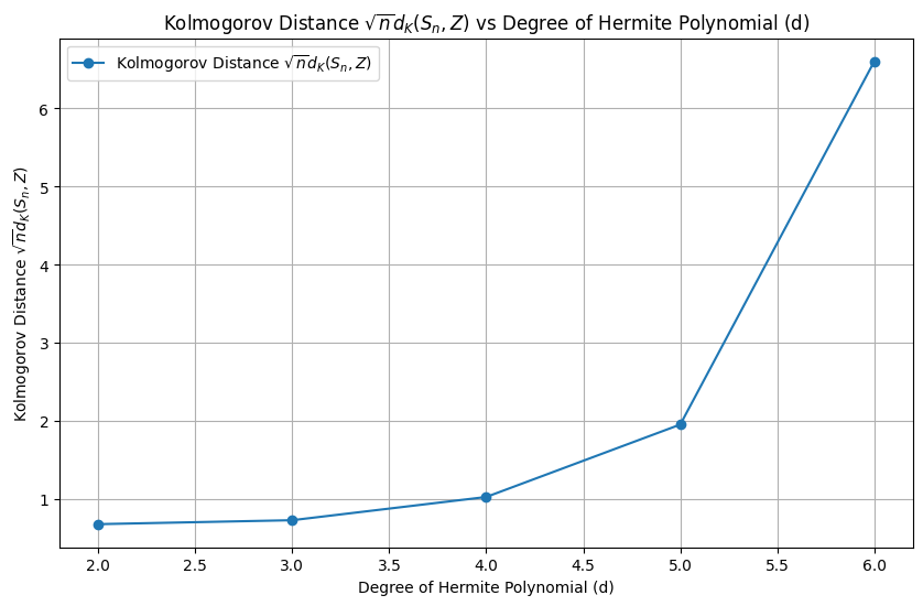
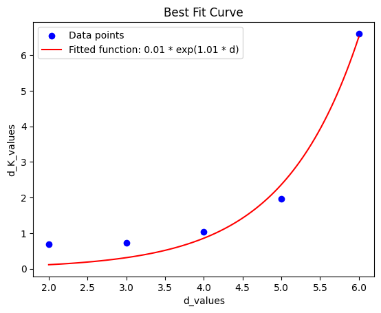
Figure 1. Plot of $d\mapsto\sqrt{n}d_{\mathcal{K}}(S_{n,d},Z_{d})$ for the values $d=2,\ldots,6$ and $n=60.000$, together with the best fitted eksponential curve.

2. Preliminaries

In this section, we introduce the most relevant results from Malliavin calculus needed in the paper. For a full monograph on Malliavin calculus, see [5]. Let $\mathfrak{H}$ be a real separable Hilbert space with inner product $\langle\cdot,\cdot\rangle_{\mathfrak{H}}$ and norm $\|\cdot\|_{\mathfrak{H}}=\langle\cdot,\cdot\rangle_{\mathfrak{H}}^{1/2}$. We call $X=\{X(h):h\in\mathfrak{H}\}$ an isormormal Gaussian process over $\mathfrak{H}$, where $X$ is defined on some probability space $(\Omega,\mathcal{F},\mathds{P})$, whenever $X$ is a centered Gaussian family indexed by $\mathfrak{H}$ such that $\mathds{E}[X(h)X(g)]=\langle h,g\rangle_{\mathfrak{H}}$. Define $\mathcal{F}$ to be the $\sigma$-algebra generated by $X$, i.e. $\mathcal{F}=\sigma\{X\}$, and write $L^{2}(\Omega,\mathcal{F},\mathds{P})=L^{2}(\Omega)$, where we say that $F\in L^{2}(\Omega)$ if $\mathds{E}[|F|^{2}]<\infty$. The Wiener-Itô chaos expansion (see [4, Cor. 2.7.8]), states, for any $F\in L^{2}(\Omega)$, that $F=\mathds{E}[F]+\sum_{q=1}^{\infty}I_{q}(f_{q})$ where $I_{0}(f_{0})=\mathds{E}[F]$, $I_{q}(f_{q})$ is the $q$’th multiple Wiener-Itô integral and the kernels $f_{q}$ are in the symmetric $q$’th tensor product in $\mathfrak{H}^{\odot q}$. For an $F\in L^{2}(\Omega)$, we write $F\in\mathbb{D}^{1,2}$ if $\sum_{q=1}^{\infty}q!q\|f_{q}\|_{\mathfrak{H}^{\otimes q}}^{2}<\infty$. For $F\in\mathbb{D}^{1,2}$ we let the random element $DF$ with values in $\mathfrak{H}$ be the Malliavin derivative, which satisfies the chain rule. Indeed, let $\bm{F}=(F_{1},\ldots,F_{d})$ where $F_{i}\in\mathbb{D}^{1,2}$ for $i=1,\ldots,d$ and let $\phi:\mathbb{R}^{d}\to\mathbb{R}$ be a continuous differentiable function with bounded partial derivatives. Then, by [5, Prop. 1.2.3], $\phi(\bm{F})\in\mathbb{D}^{1,2}$ and $D\phi(\bm{F})=\sum_{i=1}^{d}\big{(}\tfrac{\partial}{\partial x_{i}}\phi(\bm{F})\big{)}\cdot DF_{i}$.

Recall that $(G_{k})_{k\in\mathbb{N}}$ is a centered stationary Gaussian sequence with $\rho(j-k)=\mathds{E}[G_{j}G_{k}]$ and $\rho(0)=1$. By [4, Rem. 2.1.9] we may choose an isonormal Gaussian process $\{X_{h}:h\in\mathfrak{H}\}$, such that $(G_{k})_{k\in\mathbb{N}}\overset{\mathscr{D}}{=}\{X_{e_{k}}:k\in\mathbb{N}\}$ where $(e_{k})_{k\in\mathbb{N}}\subset\mathfrak{H}$ verifying $\langle e_{k},e_{j}\rangle_{\mathfrak{H}}=\rho(j-k)$ for all $j,k\in\mathbb{N}$. It then follows by [4, Thm 2.7.7] that $H_{q}(G_{r})\overset{\mathscr{D}}{=}I_{q}(e^{\otimes q}_{r})$ for all $q\geq 1$ and $r\in\mathbb{N}$. Since $D(G_{r})=e_{r}$ by [4, Rem. 2.9.2], and $H_{q}^{\prime}(x)=qH_{q-1}(x)$ by [4, Prop. 1.4.2(i)], the chain-rule implies that $DH_{q}(G_{r})=qH_{q-1}(G_{r})e_{r}$ for all $q\geq 2$ and $r\in\mathbb{N}$. Finally, the $r$th contraction operator $\otimes_{r}$ is defined in [4, App. B.4].

3. Proofs

Lemma 3.1.

Assume that $\varphi_{i}(x)=H_{i}(x)/\sqrt{i!}$ for $i=2,\ldots,d$, where $H_{i}$ is the $i$’th Hermite polynomial and that $(G_{k})_{k\in\mathbb{N}}$ is an i.i.d. stationary Gaussian sequence. For all $d\geq 2$ there exists some $N_{d}\in\mathbb{N}$ such that it for all $n\geq N_{d}$

$$d_{\mathcal{R}}(\bm{S}_{n},\bm{Z})\geq\frac{1}{\sqrt{n}(e\pi^{3}2^{3})^{1/4}}\begin{dcases}e^{3d\log(2)/2-3\log(d)/4},&\text{ if }d\text{ is even},\\ e^{3(d-1)\log(2)/2-3\log(d-1)/4},&\text{ if }d\text{ is odd}.\end{dcases}$$

Throughout the paper, we will often apply Stirling’s inequality [8, Eqs. (1) & (2)], given by

(3.1) $$\sqrt{2\pi n}\left(\frac{n}{e}\right)^{n}<n!<e^{\frac{1}{12}}\sqrt{2\pi n}\left(\frac{n}{e}\right)^{n},\quad\text{ for all }n\in\mathbb{N}.$$

Proof.

Recall that $d_{\mathcal{K}}$ is a weaker metric than $d_{\mathcal{R}}$, and hence

(3.2) $$d_{\mathcal{R}}(\bm{S}_{n},\bm{Z})\geq d_{\mathcal{K}}(\bm{S}_{n},\bm{Z})\geq\begin{dcases}d_{\mathcal{K}}(S_{n,d},Z_{d}),&\text{ if }d\text{ is even},\\ d_{\mathcal{K}}(S_{n,d-1},Z_{d-1}),&\text{ if }d\text{ is odd}.\end{dcases}$$

Here $S_{n,d}$ (resp. $S_{n,d-1}$) is the last (resp. penultimate) element of $\bm{S}_{n}$ and likewise $Z_{d}$ (resp. $Z_{d-1}$) is the last (resp. penultimate) element in $\bm{Z}$. Since the argument is now reduced to a one-dimensional problem, we will assume without loss of generality that $d$ is even and fixed. If $d$ was odd, we should just consider $d-1$ which in this case is even.

It thus suffices to find a lower bound in the one-dimensional setting $d_{\mathcal{K}}(S_{n,d},Z_{d})$. We will use [3, Thm 3.1 & Prop. 3.6] to construct such a lower bound. Since $\rho(v)=0$ for all $v\in\mathbb{Z}\setminus\{0\}$ and by [4, Prop. 2.2.1], it follows that

$$\mathrm{Var}(S_{n,d})=\frac{1}{d!n}\sum_{k,r=1}^{n}\mathds{E}[H_{d}(G_{k})H_{d}(G_{r})]=\frac{1}{n}\sum_{k,r=1}^{n}\rho(k-r)=1.$$

We now verify the assumptions in [3, Prop. 3.6]. First, we note that $S_{n,d}$ is indeed in a fixed Wiener chaos, since $S_{n,d}\overset{\mathscr{D}}{=}I_{d}\big{(}(d!n)^{-1/2}\sum_{k=1}^{n}e_{k}^{\otimes d}\big{)}\coloneqq I_{d}(f(n,d))$ for $f(n,d)\in\mathfrak{H}^{\odot d}$. To verify [3, Prop. 3.6], we start by calculating $\Psi(n)\coloneqq\mathds{E}[(1-d^{-1}\|DS_{n,d}\|_{\mathfrak{H}}^{2})^{2}]^{1/2}$, and to do so, we note that

$$\|DS_{n,d}\|_{\mathfrak{H}}^{2}=\frac{d}{(d-1)!n}\sum_{k,r=1}^{n}H_{d-1}(G_{k})H_{d-1}(G_{r})\rho(k-r)=\frac{d}{(d-1)!n}\sum_{k=1}^{n}H_{d-1}(G_{k})^{2}.$$

Hence, by definition of $\Psi(n)$, using linearity of expectations and [4, Prop.  2.2.1], it follows that

$$\Psi(n)^{2} =1-\frac{2}{(d-1)!n}\sum_{k=1}^{n}\mathds{E}[H_{d-1}(G_{k})^{2}]+\frac{1}{((d-1)!)^{2}n^{2}}\sum_{k,r=1}^{d}\mathds{E}[H_{d-1}(G_{k})^{2}H_{d-1}(G_{r})^{2}]$$

$$=-1+\frac{1}{((d-1)!)^{2}n^{2}}\left(\sum_{\underset{k\neq r}{k,r\in\{1,\ldots,n\}:}}\mathds{E}[H_{d-1}(G_{k})^{2}]\mathds{E}[H_{d-1}(G_{r})^{2}]+\sum_{k=1}^{n}\mathds{E}[H_{d-1}(G_{k})^{4}]\right)$$

$$=-1+\frac{\left(n(n-1)((d-1)!)^{2}+n\mathds{E}[H_{d-1}(G_{1})^{4}]\right)}{((d-1)!)^{2}n^{2}}=\frac{1}{n}\left(\frac{\mathds{E}[H_{d-1}(G_{1})^{4}]}{((d-1)!)^{2}}-1\right).$$

We can now verify the assumptions of [3, Eq. (3.6), (3.7) & (3.8)]. Let $s\in\{1,\ldots,d-1\}$, and note by definition of the kernels $f(n,d)$, that

$$\|f(n,d)\otimes_{s}f(n,d)\|_{\mathfrak{H}^{\otimes(2d-2s)}}^{2}=\sum_{k,k^{\prime},r,r^{\prime}=1}^{n}\frac{1}{(d!)^{2}n^{2}}\langle e_{k}^{\otimes d}\otimes_{s}e_{k^{\prime}}^{\otimes d},e_{r}^{\otimes d}\otimes_{s}e_{r^{\prime}}^{\otimes d}\rangle_{\mathfrak{H}^{\otimes(2d-2s)}},$$

where

(3.3) $$e_{k}^{\otimes d}\otimes_{s}e_{k^{\prime}}^{\otimes d}=\left(\prod_{\ell=1}^{r}\langle e_{k},e_{k^{\prime}}\rangle_{\mathfrak{H}}\right)e_{k}^{\otimes(d-s)}\otimes e_{k^{\prime}}^{\otimes(d-s)}=\begin{dcases}0,&\text{ if }k\neq k^{\prime},\\ e_{k}^{\otimes(2d-2s)},&\text{ if }k=k^{\prime}.\end{dcases}$$

Thus, since $\langle e_{k}^{\otimes(2d-2s)},e_{r}^{\otimes(2d-2s)}\rangle_{\mathfrak{H}^{\otimes(2d-2s)}}=\prod_{\ell=1}^{2d-2s}\langle e_{k},e_{r}\rangle_{\mathfrak{H}}=\mathds{1}_{\{k=r\}}$, it follows that

$$\|f(n,d)\otimes_{s}f(n,d)\|_{\mathfrak{H}^{\otimes(2d-2s)}}^{2}=\frac{1}{(d!)^{2}n}\longrightarrow 0,\quad\text{ as }n\to\infty,$$

verifying assumption [3, Eq. (3.6)]. It follows directly that $(1-d!\|f(d,n)\|_{\mathfrak{H}^{\otimes d}})/\Psi(n)=0$ for all $n\geq 2$ since $\mathrm{Var}(S_{n,d})=1$, verifying [3, Eq. (3.7)]. Next, let $s\in\{1,\ldots,d-1\}$ and $\ell\in\{1,\ldots,2d-2s-1\}$, and note by construction and symmetry of $f(n,d)$ that

$$g(n,d,s)\coloneqq f(n,d)\widetilde{\otimes}_{s}f(n,d)=\frac{1}{d!n}\sum_{k,r=1}^{n}e_{k}^{\otimes d}\otimes_{s}e_{r}^{\otimes d}=\frac{1}{d!n}\sum_{k=1}^{n}e_{k}^{\otimes(2d-2s)}.$$

By (3.3) and since $\rho(v)=0$ for all $v\in\mathbb{Z}\setminus\{0\}$, it follows that

$$g(n,d,s)\otimes_{\ell}g(n,d,s)=\frac{1}{(d!)^{2}n^{2}}\sum_{k,r=1}^{n}e_{k}^{\otimes(2d-2s)}\otimes_{\ell}e_{r}^{\otimes(2d-2s)}=\frac{1}{(d!)^{2}n^{2}}\sum_{k=1}^{n}e_{k}^{\otimes(2(2d-2s)-2\ell)}.$$

Applying this, we see that

$$\|g(n,d,s)\otimes_{\ell}g(n,d,s)\|_{\mathfrak{H}^{\otimes(2(2d-2s)-2\ell)}}\Psi(n)^{-2}$$

$$\qquad=\Psi(n)^{-2}\left(\frac{1}{(d!)^{4}n^{4}}\sum_{k,r=1}^{n}\langle e_{k}^{\otimes(2(2d-2s)-2\ell)},e_{r}^{\otimes(2(2d-2s)-2\ell)}\rangle_{\mathfrak{H}^{\otimes(2(2d-2s)-2\ell)}}\right)^{1/2}$$

$$\qquad=\frac{1}{(d!)^{2}n^{3/2}\Psi(n)^{2}}\longrightarrow 0,\quad\text{ as }n\to\infty,$$

verifying [3, Eq. (3.8)]. Finally, note by definition of $\Psi(n)$, that

$$\zeta(d) \coloneqq-dd!(d/2-1)!\binom{d-1}{d/2-1}^{2}\Psi(n)^{-1}\langle f(n,d),f(n,d)\widetilde{\otimes}_{d/2}f(n,d)\rangle_{\mathfrak{H}^{\otimes d}}$$

$$=-d(d!)^{-1/2}(d/2-1)!\binom{d-1}{d/2-1}^{2}\left(\frac{\mathds{E}[H_{d-1}(G_{1})^{4}]}{((d-1)!)^{2}}-1\right)^{-1},$$

since $f(n,d)\widetilde{\otimes}_{d/2}f(n,d)=(d!n)^{-1}\sum_{k=1}^{n}e_{k}^{\otimes d}$, which implies that $\langle f(n,d),f(n,d)\widetilde{\otimes}_{d/2}f(n,d)\rangle_{\mathfrak{H}^{\otimes d}}=(d!)^{-3/2}n^{-1/2}$. Note that $\zeta(d)$ purely depends on $d$, and hence does not depend on $n$.

Applying [3, Thm 3.1 & Prop. 3.6], it now follows that there exists some $N_{d}\in\mathbb{N}$ such that

$$d_{\mathcal{K}}(S_{n,d},Z_{d})\geq\frac{3}{\sqrt{2\pi}}\Psi(n)|\zeta(d)|,\quad\text{ for all }n\geq N_{d}.$$

The proof can now be concluded, by using the definition of $\zeta(d)$ and multiple applications of Stirling’s approximation (3.1) to get a lower bound on $\Psi(n)|\zeta(d)|$:

$$\sqrt{n}\Psi(n)|\zeta(d)| =\frac{d(d/2-1)!\binom{d-1}{d/2-1}^{2}}{\sqrt{d!}}=\frac{\sqrt{d!}(d-1)!}{(d/2-1)!((d/2)!)^{2}}$$

$$\geq\frac{1}{(2e\pi^{3})^{1/4}}\left(\frac{d-2}{d-1}\right)^{1/2}\frac{(d-1)^{d}}{d^{d/2}(d-2)^{d/2}}\frac{2^{3d/2}}{d^{3/4}}\geq\frac{1}{(2^{3}e\pi^{3})^{1/4}}e^{3d\log(2)/2-3\log(d)/4}.\qed$$

To prove the main results, we recall the following fourth-moment bound on the Hermite polynomials from [1, Lem. 5.2].

Lemma 3.2 ([1, Lem. 5.2]).

Let $\ell\geq 2$, $H_{\ell}$ be the $\ell$’th Hermite polynomial and $G\sim\mathcal{N}(0,1)$. Then, there exists a uniform constant $c>0$, such that

(3.4) $$\mathds{E}[H_{\ell}(G)^{4}]^{1/4}\leq c\ell^{\ell/2}e^{\ell(\log(3)/2-1/2)}\ell^{1/4},\quad\text{ for all }\ell\geq 2.$$

Proof of Theorem 1.1.

Assume now that $(G_{k})_{k\in\mathbb{N}}$ is an i.i.d. stationary Gaussian sequence. We start by proving the lower bound in (1.5). For all $d\geq 2$, Lemma 3.1 implies that there exists some $N_{d}\in\mathbb{N}$ such that it for all $n\geq N_{d}$

$$d_{\mathcal{R}}(\bm{S}_{n},\bm{Z})\geq\frac{1}{\sqrt{n}(e\pi^{3}2^{3})^{1/4}}\begin{dcases}e^{3(d+1)\log(2)/2-3\log(d+1)/4},&\text{ if }d\text{ is even},\\ e^{3d\log(2)/2-3\log(d)/4},&\text{ if }d\text{ is odd}.\end{dcases}$$

Thus, since $\log(d+1)\geq\log(d)$, it follows that

(3.5) $$d_{\mathcal{R}}(\bm{S}_{n},\bm{Z})\geq\frac{e^{3\log(2)/2}}{(e\pi^{3}2^{3})^{1/4}}\frac{e^{3d\log(2)/2}}{d^{3/4}\sqrt{n}},\qquad\text{ for all }n\geq N_{d}.$$

Now, for all $\varsigma<3\log(2)/2$ there exists some $C_{\varsigma}$, such that for all $d\geq 2$, it holds that $d_{\mathcal{R}}(\bm{S}_{n},\bm{Z})\geq C_{\varsigma}e^{\varsigma d}/\sqrt{n}$ for all $n\geq N_{d}$, concluding the proof of the lower bound.

Next, we prove the upper bound in (1.5). Note that $\mathrm{Cov}(\bm{S}_{n})=\mathrm{Cov}(\bm{Z})=\bm{I}_{d}$, since the orthogonality of the Hermite polynomials yields $\mathrm{Cov}(\bm{S}_{n})_{i,j}=0$ if $i\neq j$ and moreover if $i=j$ the assumption of i.i.d. together with [4, Prop. 2.2.1] yields

$$\mathrm{Cov}(\bm{S}_{n})_{i,i}=\mathrm{Var}\left(\frac{1}{\sqrt{n}}\sum_{k=1}^{n}\frac{H_{i+1}(G_{k})}{\sqrt{(i+1)!}}\right)=\frac{1}{n}\sum_{k,k^{\prime}=1}^{n}\frac{\mathds{E}[H_{i+1}(G_{k})H_{i+1}(G_{k^{\prime}})]}{(i+1)!}=\frac{1}{n}\sum_{k,k^{\prime}=1}^{n}\rho(k-k^{\prime})=1.$$

Hence, by [2, Thm 1.1] and Jensen’s inequality, there exists some absolute positive constant $c$ (which exact value can be found in [7, Thm 1.1]), such that

(3.6) $$d_{\mathscr{C}}(\bm{S}_{n},\bm{Z})\leq\frac{cd^{1/4}}{\sqrt{n}}\mathds{E}\left[\left(\sum_{i=1}^{d}\varphi_{i}(G_{1})^{2}\right)^{3/2}\right]\leq\frac{cd^{3/4}}{\sqrt{n}}\sum_{i=1}^{d}\mathds{E}[|\varphi_{i}(G_{1})|^{3}],$$

where we recall that $\varphi_{i}(x)=H_{i+1}(x)/\sqrt{(i+1)!}$. Thus, it suffices to bound $\mathds{E}[|\varphi_{i}(G_{1})|^{3}]$ in terms of $i$. Applying Jensen’s inequality, Lemma 3.2 and (3.1) yields the existence of a constant $\widehat{c}>0$, such that

$$\frac{\mathds{E}[|H_{i}(G_{1})|^{3}]}{(i!)^{3/2}}\leq\frac{\mathds{E}[H_{i}(G_{1})^{4}]^{3/4}}{(i!)^{3/2}}\leq\left(\frac{\widehat{c}i^{i/2}e^{i(\log(3)/2-1/2)}i^{1/4}}{\sqrt{i!}}\right)^{3}\leq\frac{\widehat{c}^{3}}{(2\pi)^{3/4}}e^{i(3\log(3)/2)},$$

for $i=2,\ldots,d+1$. Using the closed form for partial geometric series, it follows altogether that there exists some absolute constant $K$ such that

(3.7) $$d_{\mathscr{C}}(\bm{S}_{n},\bm{Z})\leq\frac{Kd^{3/4}}{\sqrt{n}}\sum_{i=1}^{d}e^{i(3\log(3)/2)}\leq\frac{Ke^{3\log(3)/2}}{e^{3\log(3)/2}-1}\frac{d^{3/4}e^{d(3\log(3)/2)}}{\sqrt{n}}.$$

Hence, for any $\widetilde{\varsigma}>3\log(3)/2$ there exists a constant $\widetilde{c}$ which depends on $\widetilde{\varsigma}$, such that $d_{\mathcal{R}}(\bm{S}_{n},\bm{Z})\leq\widetilde{c}e^{\widetilde{\varsigma}d}$ for all $d\in\mathbb{N}$, concluding the proof. ∎

References

• Basse-O’Connor and Kramer-Bang [2025] Basse-O’Connor, A. and D. Kramer-Bang (2025). Quantative bounds for high-dimensional non-linear functionals of Gaussian processes. Preprint.
• Bentkus [2004] Bentkus, V. (2004). A Lyapunov type bound in ${\bf R}^{d}$. Teor. Veroyatn. Primen. 49(2), 400–410.
• Nourdin and Peccati [2009] Nourdin, I. and G. Peccati (2009). Stein’s method and exact Berry-Esseen asymptotics for functionals of Gaussian fields. Ann. Probab. 37(6), 2231–2261.
• Nourdin and Peccati [2012] Nourdin, I. and G. Peccati (2012). Normal approximations with Malliavin calculus, Volume 192 of Cambridge Tracts in Mathematics. Cambridge University Press, Cambridge. From Stein’s method to universality.
• Nualart [2006] Nualart, D. (2006). The Malliavin calculus and related topics (Second ed.). Probability and its Applications (New York). Springer-Verlag, Berlin.
• Plucińska [1999] Plucińska, A. (1999). Some properties of polynomial-normal distributions associated with Hermite polynomials. Demonstratio Math. 32(1), 195–206.
• Raič [2019] Raič, M. (2019). A multivariate Berry-Esseen theorem with explicit constants. Bernoulli 25(4A), 2824–2853.
• Robbins [1955] Robbins, H. (1955). A remark on Stirling’s formula. Amer. Math. Monthly 62, 26–29.