Ancilla theory of twisted bilayer graphene I: topological Mott semimetal and symmetric pseudogap metal

Abstract

In this work, we demonstrate that Mott physics in twisted bilayer graphene (TBG) can be conveniently captured using the ancilla theory, originally proposed in the context of high-Tc cuprates [Zhang and Sachdev, Phys. Rev. Res. 2, 023172 (2020)] . In this framework, the Mott gap emerges as a band gap at the mean-field level, controlled by a hybridization order parameter $\Phi(\mathbf{k})$ between the physical and ancilla bands. The conventional Hubbard bands naturally arise from an s-wave-like hybridization $\Phi(\mathbf{k})=\frac{U}{2}$. In TBG, the ancilla formalism allows us to calculate the upper and lower Hubbard bands directly in momentum space, both at and away from the magic angle. Projected to the active bands, we reveal a topological obstruction for $\Phi(\mathbf{k})$ around the $\Gamma$ point, leading to a topological Mott semi-metal at $\nu=0$. At fillings $\nu=\pm 1,\pm 2,\pm 3$, we obtain symmetric correlated insulators at large $U$, and also transitions to semi-metals at smaller $U$ or larger bandwidth. The new formalism also enables us to study the most intriguing density range, $\nu=-2-x$: we propose a symmetric pseudogap metal at small $x$, which hosts a small Fermi surface and violates the perturbative Luttinger theorem. Our theory works above the ordering temperature of a potential symmetry-breaking order. Alternatively, the symmetric pseudogap metal can survive to the zero-temperature limit when there is a sizable anti-Hund’s coupling $J_{A}$ mediated by optical phonons. In this case we can write down a variational wavefunction within the subspace of active bands. In our theory, the small Fermi surface of the pseudogap metal is primarily formed by ancilla fermions, which we interpret as composite polarons—consisting of a spin moment on an AA site bound to a hole in the nearest neighbor AA site. Within the active band subspace, the composite polaron at $\mathbf{k}=0$ is orthogonal to the single-particle state due to their differing angular momenta, and thus has vanishing spectral weight. We suggest that superconductivity emerges from the Cooper pairing of these composite fermions instead of single electrons.

Introduction Discoveries of correlated insulators and superconductivity in the magic angle twisted bilayer graphene (TBG) [1, 2, 3, 4, 5, 6, 7, 8] and twisted multilayer graphene[9, 10, 11, 12] have attract lots of attentions in recent years and initiated a whole new area of moiré materials[13, 14, 15]. Although the phase diagram of TBG has certain similarity to that of the high temperature superconducting cuprates, theoretical studies indicate that the physics is different from a conventional Hubbard model due to the fragile band topology [16, 17, 18, 19, 20]. As a result, it is not clear whether Mott physics really matters in the system. The previous theoretical studies have focused on quantum Hall physics and various symmetry breaking phases (such as inter-valley coherent orders)[21, 22, 23, 24]. Indeed experiments observed integer quantum anomalous Hall effects[25, 26] when TBG is aligned with a hexagon boron nitride (hBN)[27, 28] and even fractional Chern insulator (FCI) phases at finite magnetic field[29]. Hence one may tend to conclude that the TBG physics is far away from high Tc cuprate physics. However, there are also experimental evidences of local moments at finite temperature ($T$) from entropy measurements[30, 31], indicating Mott localization.

To describe the Mott physics theoretically, there have been attempts to construct single particle basis with Wannier orbital on the AA site. The first approach is through the topological heavy fermion model (THFM) [32, 33, 34, 35, 36, 37, 38, 39, 40, 41, 42, 43] which includes both the active bands and the remote bands, so localized orbital is possible. In the second approach, one can construct non-local Wannier orbital only for the active bands[44], but the interaction may not be easily truncated to a simple on-site Hubbard $U$. In this work we follow a different approach. Instead of searching for a good single particle basis with localized orbital, we will propose a new many-body theory of Mott physics which can be formulated directly in the continuum model.

Our framework is a generalization of the ancilla theory[45, 46] originally proposed in the context of the standard spin 1/2 Hubbard model to the TBG model. In the ancilla framework, we introduce two additional layers of ancilla fermions $\psi_{i;\alpha}$ and $\psi^{\prime}_{i;\alpha}$, where $i$ labels a real space lattice site where the ‘local moment’ lives. In TBG we will put $\psi_{i}$ and $\psi^{\prime}_{i}$ both on the AA site. $\alpha$ is the flavor index of a SU(N) fermion. Then a physical state can be written as:

$$|\Psi_{c}\rangle=P_{S}|\Psi_{0}[c,\psi,\psi^{\prime}]\rangle.$$ (1)

Here, $|\Psi_{0}[c,\psi,\psi^{\prime}]\rangle$ is a variational state in the enlarged Hilbert space and $P_{S}$ is a projection operator which enforces the two ancilla fermions to form a SU(N) spin-singlet at each site $i$, as illustrated in Figs. 1(a) and (c). The physical layer $c$ and the first ancilla layer $\psi$ are coupled through a hybridization $\Phi(\mathbf{k})c^{\dagger}_{\mathbf{k};\alpha}\psi_{\mathbf{k};\alpha}$ to open a charge gap, while the spin state is encoded in the second ancilla layer $\psi^{\prime}$ which represents the local moments. The validity of this seemingly exotic wavefunction for the Mott insulator of spin-1/2 Hubbard model at half filling has been demonstrated both analytically and numerically [46]. For example, we should set $\Phi(\mathbf{k})=\frac{U}{2}$ at large $U$ limit. The large hybridization enforces $c_{i}$ and $\psi_{i}$ to form an Einstein–Podolsky–Rosen (EPR) pair. Then the projection $P_{S}$ is equivalent to a Bell measurement and the spin state in $\psi^{\prime}$ is quantum teleported to the physical layer. In the end we obtain a wavefunction equivalent to the inverse Schriffer-Wolff transformation at leading order of $t/U$ expansion[46]. Variational monte carlo studies[47, 48] also demonstrated that the ancilla wavefunction can correctly capture the polaronic correlations in doped Mott insulator.

In the ancilla formalism, there is no requirement for the physical electron to have a lattice model description. So we can describe the Mott physics in TBG directly in the continuum model, though the same results can be obtained in the basis of THFM. At $\nu=0$, we obtain a topological Mott semimetal with quadratic band touching at $\Gamma_{M}$ point. This state was already discussed in Ref. [44] based on self energy calculation, but now we can provide an effective theory to capture the band topology and also write down model wavefunction at $T=0$. At $\nu=\pm 1,\pm 2,\pm 3$, we predict transitions from correlated insulators to semi-metals by reducing $U$ or increasing the twist angle. To our best knowledge, the Mott semimetal at non-zero integer filling is a new result.

The most exciting discovery is a symmetric pseudogap metal at filling $\nu=-2-x$ with small $x$. We find a small Fermi surface state similar to the pseudogap metal in the ancilla theory of the underdoped cuprate[45]. But a new feature arises due to the band topology of the TBG. The quasi particle of the small Fermi surface is dominated by the ancilla Fermion $\psi$ at small $x$, and thus has vanishing spectral weight. Hence a gap will be observed in single electron spectroscopy measurement, despite that there is actually a Fermi surface with large effective mass $m^{*}\sim m_{e}$. We interpret the ancilla fermion as a composite polaron or composite trion, formed by a spin moment on AA site bound to a hole in the nearest neighbor AA site. We suggest that the normal state of the superconductor is this pseudogap metal formed by the composite polarons. This implies that a successful theory of superconductivity must be formulated in terms of these composite fermions instead of single electrons. As far as we can see, the ancilla approach is the only possible way to formulate a low energy effective theory of these composite fermions.

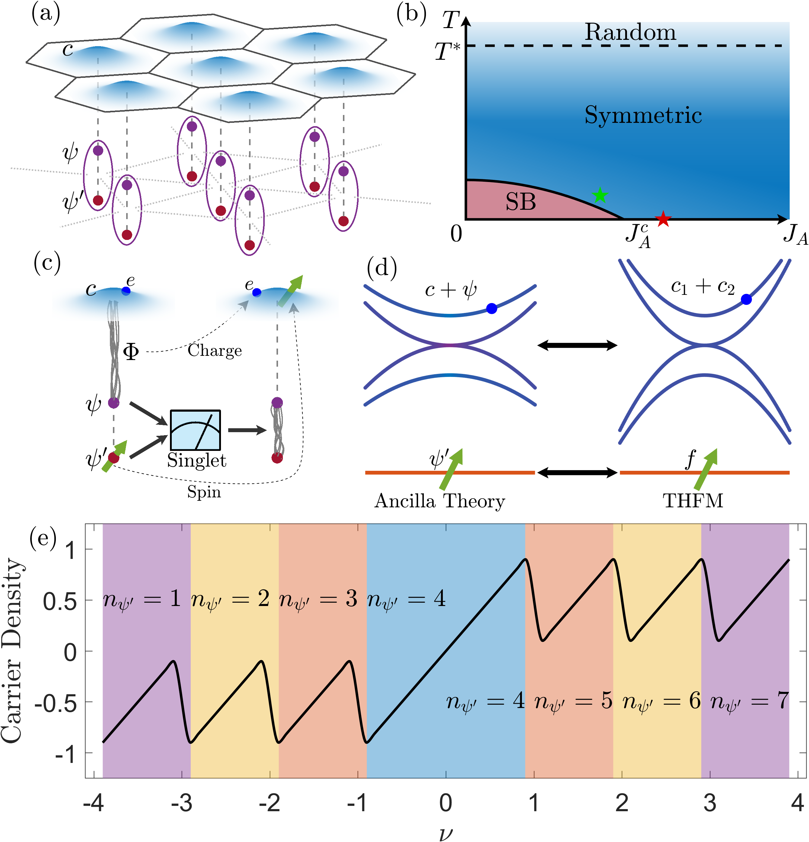
Figure 1: (a) Illustration of the ancilla wavefunction in the TBG system. The top layer is the physical TBG layer with the active band density centered at AA positions (blue wave packet). The bottom two layers are the first ancilla $\psi$ (purple) and the second ancilla $\psi^{\prime}$ (orange), respectively, also located at AA positions. (b) An illustration of the phase diagram of the inter-valley interaction $J_{A}$ and temperature $T$. Our symmetric ansatz applies for all the blue regime, except for the symmetry breaking (SB) phase $J_{A}<J_{A}^{c}$ and the incoherent phase $T>T^{*}$. (c) At each AA site, the wavefunction is projected back to the physical Hilbert space by enforcing the two ancilla fermions to for a SU(8) spin singlet. (d) At low energy, we have an emergent charge sector formed by $c,\psi$ and local moments represented by $\psi^{\prime}$, which seems to have one to one correspondence in the THFM, but with different physical meanings. (e) illustrates the number occupancy of the second ancilla $n_{\psi^{\prime}}$ at the physical filling $\nu$. We always have $n_{i;\psi}+n_{i;\psi^{\prime}}=8$ at each AA site labeled by $i$. At each integer filling $n_{c}=4+\nu$, we choose $n_{\psi}=4-\nu$ and $n_{\psi^{\prime}}=4+\nu$ so that the ancilla wavefunction describes a Mott localized state. At fractional filling such as $\nu\in(-3,-2)$, we can in principle use the ancilla wavefunction with either $n_{\psi^{\prime}}=2$ or $n_{\psi^{\prime}}=1$, which correspond to doping the parent state at $\nu=-2$ or $\nu=-3$ respectively. Here we simply assume the ansatz switches from the $\nu=-2$ parent state to $\nu=-3$ parent state close to $\nu=-3$ to match the experimental observations. This reset of the carrier density is assumed to be a first-order transition with $n_{\psi^{\prime}}$ jumping by $1$ in our theory.

General formalism The ancilla wavefunction in Eq. (1) can be directly generalized to the TBG system. In the TBG, there are 8 active bands labeled by the valley $\tau=K,K^{\prime}$, the spin $s=\uparrow,\downarrow$, and the orbital $a=+,-$. Then we introduce SU(8) ancilla fermions $\psi_{i;a\tau s}$ and $\psi^{\prime}_{i;a\tau s}$ living on the AA site labeled by $i$. The projection operator $P_{S}$ enforces $\psi$ and $\psi^{\prime}$ to form an SU(8) singlet at each site $i$. There are three constraints: (I) We fix $n_{i;\psi^{\prime}}=n$ with $n$ to be an integer at each site $i$. So the second ancilla $\psi^{\prime}$ just represents a fully localized spin state in the $n_{T}=n$ representation of the SU(8) spin. (II) We fix $n_{i;\psi}=8-n$ at each site $i$. (III) We fix $S^{\alpha\beta}_{i;\psi}+S^{\alpha\beta}_{i;\psi^{\prime}}=0$ at each site $i$. Here $S^{\alpha\beta}$ with $\alpha,\beta=1,2,...,8$ labels each spin operator of SU(8). These three constraints give a $U(1)\times U(1)\times SU(8)$ gauge symmetry. But we will only consider the ansatz where all of the gauge fields are higgsed, so we can ignore the gauge symmetry in this work. At integer filling $\nu$ with total density $n_{c}=4+\nu$, we should set $n_{i;\psi^{\prime}}=4+\nu$ and $n_{i;\psi}=4-\nu$ to capture a Mott state. Away from the integer filling, we expect $n_{i;\psi^{\prime}}$ to stay in the integer associated with the parent Mott state. In this picture the reset of the carrier density close to an integer $\nu$ is associated with a jump of $n_{i;\psi^{\prime}}$ by $1$ (see Fig. 1(e)).

In the ancilla description of a Mott state, we always have the charge sector formed by $c,\psi$ and the neutral spin sector from $\psi^{\prime}$. In this work we assume the spin state of $\psi^{\prime}$ is symmetric. In reality there should be an effective ferromagnetic spin-spin coupling between the local moments $J<0$, so one may worry that the true ground state is ordered. Our following discussion is then justified for two regimes (see Fig. 1(b)): (I) We consider finite temperature with $|J|\ll T\ll U$, where the local moments in $\psi^{\prime}$ layer is just thermally fluctuating, but the charge sector of $c,\psi$ still behave like a low-temperature state. (II) We can add an additional spin-spin coupling term, for example, an anti-Hund’s coupling $J_{A}\sum_{\mathbf{q}}\vec{S}_{\mathbf{K}}(\mathbf{q})\cdot\vec{S}_{\mathbf{K}^{\prime}}(-\mathbf{q})$ [50] which enforces inter-valley spin-singlet when $n_{\psi^{\prime}}$ is even. Such a $J_{A}$ coupling can be mediated by optical phonons at momentum $K$[51]. In this case we can have a symmetric spin state as a ground state and then we can provide variational wavefunctions for symmetric Mott semimetal/insulator at $\nu=-2$ and a symmetric pseudogap metal at $\nu=-2-x$. In the following we will mainly focus on the charge sector and provide mean field theory of $c,\psi$. Our formulation has the advantage of being basis independent and we can obtain equivalent results in continuum model and in THFM.

Continuum model We can construct the Wannier orbital of $\psi_{i;a\tau s}$ as a $\delta$ function located at AA positions $i$ of TBG for each valley $\tau$, spin $s$, and orbital $a$. The mean field Hamiltonian takes the form:

$${H}_{\mathrm{MF}}^{(c\psi)}={H}_{\mathrm{BM}}-\mu_{c}N_{c}-\mu_{\psi}N_{\psi}+{H}_{\mathrm{hyb}}^{(c\psi)}~.$$ (2)

Here the physical electron is described by the continuum Bistritzer-MacDonald (BM) model[52], denoted as ${H}_{\mathrm{BM}}$, which is briefly reviewed in Appendix B. The ancilla $\psi$ is assumed to be completely flat with only a chemical potential term. The hybridization term is given by:

$${H}_{\mathrm{hyb}}^{(c\psi)}=\Phi_{0}\sum_{l,\mathbf{k}\in\mathrm{MBZ},\mathbf{G}_{M}}e^{i\frac{\pi}{4}la}c^{\dagger}_{0,\mathbf{k}+\mathbf{G}_{M};la\tau s}\psi_{\mathbf{k};a\tau s}+\mathrm{h.c.}~,$$ (3)

where $\mathbf{G}_{M}$ is the moiré reciprocal vector and $\Phi_{0}$ is the strength of the hybridization which should scale with $U$. Note $l$ is the layer index and $c_{0,\mathbf{k};la\tau s}$ labels the single electron state in the original graphene lattice scale, which will be folded to the mini Brillouin zone (MBZ) by $H_{\mathrm{BM}}$. We also need to emphasize that $\psi_{i;a=\pm}$ has angular momentum $L=\pm 1$ under $C_{3z}$ rotation around the AA site.

Topological heavy fermion model In the THFM, for each flavor $\alpha=a\tau s$, there is a flat and localized $f$ band and itinerant $c_{1},c_{2}$ bands. $c_{1},c_{2}$ form an effective model similar to the K valley of the AB stacked bilayer graphene. There is a large hybridization $\gamma c^{\dagger}_{1,\mathbf{k}}f_{\mathbf{k}}$ which opens the remote gap. In the end, the active bands are mainly from the localized $f$ states except around $\Gamma_{M}$ point where it is dominated by $c_{2}(\bf k)$ with angular momentum $L=0$. $f$ state has angular momentum $L=\pm 1$ around the AA site. Assuming the Mott localization happens due to Hubbard $U$ on the $f$ orbital, we introduce $\psi_{i}$ and $\psi^{\prime}_{i}$ with the same Wannier orbital as $f$. The mean field theory of the charge sector is:

$$\begin{split}H_{\mathrm{MF}}^{(cf\psi)}=&H_{\mathrm{THFM}}+\Phi\sum_{i,a,\tau,s}\left(f^{\dagger}_{i;a,\tau,s}\psi_{i;a,\tau,s}+\mathrm{H.c.}\right)\\ &-\mu(N_{c_{1}}+N_{c_{2}}+N_{f})-\mu_{\psi}N_{\psi},\end{split}$$ (4)

where $N_{c_{1}},N_{c_{2}},N_{f},N_{\psi}$ represent the total density of $c_{1},c_{2},f,\psi$ electrons respectively. $\mu_{\psi}$ is introduced to fix the gauge constrain $n_{i;\psi}=n$, but now we relax the constrain on average.

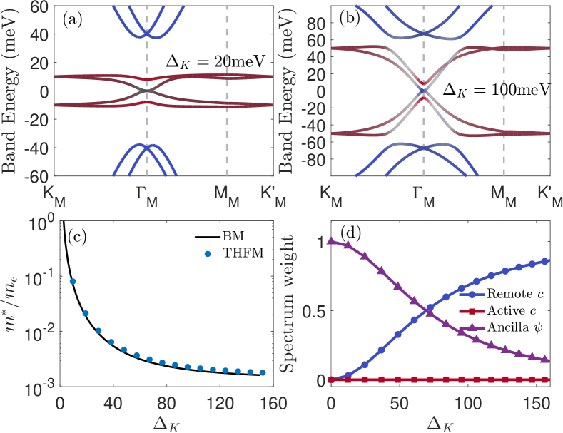
Figure 2: Mott bands calculated by BM model at $\nu=0,\theta=1.14^{\circ},w_{0}/w_{1}=0.8$, for different hybridization at (a) $\Delta_{K}=20$ meV and (b) $\Delta_{K}=100$ meV, where $\Delta_{K}$ is $K_{M}$ point Mott gap. The red, blue and dark colors of the dispersion line represent the weight of the active band, the remote bands and the ancilla bands, respectively. In (c), we show the effective mass $m^{*}/m_{e}$ of the gapless $\Gamma_{M}$ point as a function of the $K_{M}$ point gap $\Delta_{K}$. We also show the results from THFM. (d) The $\Gamma_{M}$ point spectral weights coming from the active band, remote bands, and ancilla band as a function $\Delta_{K}$.

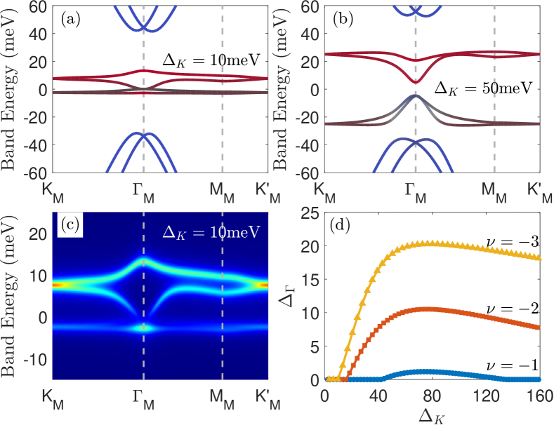
Figure 3: Mott bands calculated by BM model at $\nu=-2,\theta=1.14^{\circ},w_{0}/w_{1}=0.8$ for different hybridization strengths at (a) $\Delta_{K}=10$ meV, and (b) $50$ meV, respectively, where $\Delta_{K}$ is the $K_{M}$ point band gap. The colors has the same meaning as in Figs. 2 (a) and (b). (c) shows the corresponding physical spectrum function $A_{c}(\mathbf{k},\omega)$ at $\Delta_{K}=10$ meV. A broading of $\eta=1$ meV is used in getting the result. And (d) shows the $\Gamma_{M}$ point gap $\Delta_{\Gamma}$ as a function of the $K_{M}$ point gap $\Delta_{K}$ and filling $\nu$, which characterize the semi-metal to insulator transition.

Topological Mott semimetal at $\nu=0$ At $\nu=0$. The mean field spectrum is shown in Figs. 2 (a)-(b) for different hybridization strength, corresponding to different values of $U$. Here we use the gap at $K_{M}$ point, $\Delta_{K}$ to characterize the hybridization. $\Delta_{K}\propto\Phi$ and should be viewed as a variational parameter to be optimized for each $U$. In large $U$ limit we expect $\Delta_{K}=U$, but $\Delta_{K}$ can be smaller than $U$ close to the Mott transition. All the results are calculated at a twist angle $\theta=1.14^{\circ}$ and $w_{0}/w_{1}=0.8$. Away from $\Gamma_{M}$ point, we find upper and lower Hubbard bands just as in a conventional Hubbard model. In the large $U$ limit, we find that the four bands around $\Gamma_{M}$ are basically the same as the $c_{1},c_{2}$ bands in the topological heavy fermion model (THMF) (see the supplementary). Thus our ancilla theory can recover the result in the $\gamma\ll U$ limit of the THFM directly in the continuum model. When decreasing $U$ (or equivalently $\Delta_{K}$), the quadratic touching crossovers from the $c_{1}$ band in THFM to the ancilla $\psi$. One can see that the effective mass $m^{*}$ increases by two orders of magnitudes (see Fig. 2(c)) and the physical spectral weight $Z$ vanishes (see Fig. 2(d)) when we reach the limit $U\ll\gamma$. The calculations in continuum model and in THFM basis give the same results (see the supplementary).

Effective theory around $\mathbf{k}=0$ When $U\ll\gamma$, we can do the calculation projected into the active band. The active bands can be decomposed into two Chern bands $C=\pm 1$ labeled by $c_{\mathbf{k};\pm}$[19]. The hybridization between $c_{\mathbf{k}}$ and $\psi_{\mathbf{k}}$ are then constrained to have a node $\Phi(\mathbf{k})\sim k_{x}\pm ik_{y}$ around $\Gamma_{M}$ point, while $\Phi(\mathbf{k})=\frac{U}{2}$ away from $\Gamma_{M}$. Within each spin-valley flavor, we can then easily write down an effective four-band model close to $\mathbf{k}=0$ in terms of $c=(c_{+},c_{-})$ and $\psi=(\psi_{+},\psi_{-})$:

$${H}^{(c\psi)}_{\Gamma_{M}}= \sum_{\mathbf{k}}c^{\dagger}_{\mathbf{k}}M\sigma_{x}c_{\mathbf{k}}+\sum_{\mathbf{k}}c^{\dagger}_{\mathbf{k}}\Phi_{\Gamma}(k_{x}\sigma_{0}+ik_{y}\sigma_{z})\psi_{\mathbf{k}}+\mathrm{h.c.}$$ (5)

where $\sigma_{a}$ labels the Pauli matrix in orbital space and $W=2M$ gives the bandwidth of the active bands. $\Phi_{\Gamma}$ is proportional to $\Delta_{K}$. The effective model is equivalent to the $K$ corner of the AB stacked bilayer graphene if we treat $a=+,-$ as ‘layer’. When $M$ is finite, there is a quadratic band crossing mainly from $\psi$ with dispersion $\epsilon_{\pm}(\mathbf{k})\approx\frac{\Phi_{\Gamma}^{2}}{M}k^{2}$. Although $\psi$ has vanishing spectral weight $Z$, it responds to electric-magnetic field just like an electron because we are in a Higgs phase[45]. So we expect the Landau level degeneracy sequence of $\pm 4,\pm 8,\pm 12,...$ at energy scale below $M$. In the chiral limit with $M=0$, we have two decoupled Dirac cones in each spin-valley.

Correlated insulators and semimetals at non-zero integer fillings For other integer fillings, we get a gapped insulator for intermediate $U$. Then when decreasing $U$, the correlated insulator transits to a semi-metal at a critical $U_{c}$ (or equivalently $\Delta^{c}_{K}$). We show the Hubbard bands for $\nu=-2$ in Fig. 3 (a)-(b). For $\Delta_{K}<\Delta_{K}^{c}\approx 16$ meV, there is a quadratic band crossing at $\mathbf{k}=0$, though it is invisible in single electron spectral function $A_{c}(\omega,\mathbf{k})$, as shown in Fig. 3(c). The insulator to semimetal transition also happens for $\nu=\pm 1,\pm 3$, as we show in Fig. 3(d).

The gap in the correlated insulator is not from the Mott gap. The mean field Hamiltonian around $\mathbf{k}=0$ is still the same as Eq. (5), but now we need to adjust $\mu_{\psi}$ to fix $n_{\psi}=4-\nu$. This gives an energy shift $\Delta_{\psi}$ of the $\psi$ band relative to the physical band. For large $U$, we should use $\Delta_{\psi}=\frac{\nu}{4}\Delta_{K}$. The negative $\Delta_{\psi}$ gives the gap in Fig. 3(b). At smaller $\Delta_{K}$, $\Delta_{\psi}$ deviates from $\frac{\nu}{4}\Delta_{k}$ and the two states from $\psi$ move to the middle around $\mathbf{k}=0$, forming a quadratic band touching similar to $\nu=0$. Though it may not be relevant to realistic system, we point out that there is also a gap closing transition in the $U\gg\gamma$ limit ($\gamma$ is the remote band gap), which can be understood as a relative energy shift of the $c_{1}$ band from $\frac{\gamma^{2}}{U}$ perturbation calculation (see the supplementary) in the THFM. Again our ancilla theory can reproduce the same result in continuum model.

Symmetric pseudogap metal at $\nu=-2-x$ Now we try to dope the $\nu=-2$ insulator or semimetal. In the ancilla theory we still keep $n_{i;\psi}=6$ and $n_{i;\psi^{\prime}}=2$ at small $x$ . In this case we find a small Fermi surface from holes doped into the lower Hubbard band at $\nu=-2$, which coexists with the local moments in the $\psi^{\prime}$ layer. We show the plots of the band and physical spectral function $A_{c}(\omega,\mathbf{k})$ for two values of $\Delta_{K}$ in Fig. 4(a-d). When doping the correlated insulator, we get two Fermi surfaces within each spin-valley flavor. On the other hand, there is only one Fermi surface when slightly doping the semimetal. We note that $\Delta_{K}$ likely decreases with the doping $x$, so we should use a smaller $\Delta_{K}$ even if $\Delta_{K}$ is large at $\nu=-2$. For $\Delta_{K}=5$ meV, we provide momentum integrated spectral function $A_{c}(\omega)$ for a range of $x$ in Fig. 4(e). We can see that the spectral weight in the $\omega<0$ side is smaller than the $\omega>0$ side, which actually was also observed in the scanning tunneling microscope (STM) experiment in the pseudogap region[53]. For the same value of $\Delta_{K}$, the effective mass $m^{*}$ reaches order of electron mass $m_{e}$ (see Fig. 4(f)), which also agrees with the experimental estimation from quantum oscillations[1].

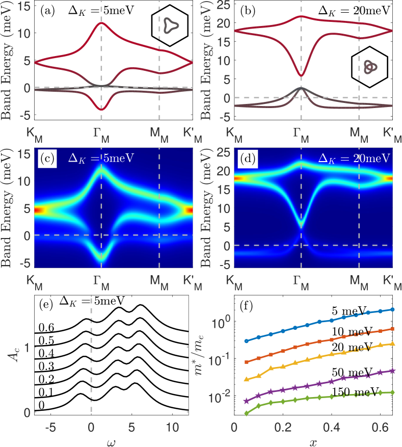
Figure 4: Mott bands calculated by BM model with doping $\nu=-2-0.4$ and $\theta=1.14^{\circ},w_{0}/w_{1}=0.8$, for different hybridization at (a) $\Delta_{K}=5$meV and (b) $\Delta_{K}=20$ meV, where $\Delta_{K}$ is defined as the $K_{M}$ point gap. The corresponding Fermi surface are also shown in the insets. (c) and (d) shows the physical electron spectrum function $A_{c}(\mathbf{k},\omega)$ with same parameters as in (a) and (b). And in (e), we show the STM spectrum $A_{c}(\omega)=\sum_{\mathbf{k}}A_{c}(\mathbf{k},\omega)$ at $\Delta_{K}=5$ meV for different dopings $\nu=-2-x$, $x=0-0.6$, with a slightly vertical shift for each $x$. A broading $\eta=1$ meV is used to get the spectrum functions $A_{c}(\mathbf{k},\omega)$ and $A_{c}(\omega)$. (f) shows the Fermi surface effective mass $m^{*}/m_{e}$ as a function of doping $\nu=-2-0.4$ for different hybridization $\Delta_{K}$. Here the effective mass $m^{*}$ is estimated by the Fermi surface density of states.

The quasi particle at the Fermi surface is dominated by the ancilla fermion $\psi$ at small $x$. Actually the spectral function $A_{c}(\omega,\mathbf{k})$ almost looks like that there is a gap (see Fig. 4(c)), though there is actually a quite flat band formed by the ancilla $\psi$. This raises the question: what is the physical meaning of the ancilla fermion? In the supplementary we show that $\psi$ is real and represents a many-body excitation. At $\mathbf{k}=0$, at leading order it corresponds to a composite polaron formed by a spin on AA site bound to a hole on the nearest neighbor AA site. Such a composite fermion is orthogonal to the single particle state at $\mathbf{k}=0$ due to different angular momenta under $C_{3z}$ rotation. We emphasize that this polaron emerges once the Mott localization (a non-zero $\Phi$) is developed below $T^{*}$ and does not depend on any specific spin state, which may be different from previous discussions[54, 55, 56] of spin polarons on top of specific magnetic orders.

In our current description, the Fermi surface degeneracy is four-fold, which disagrees with the two-fold degeneracy in experiments. We note that there is likely an additional symmetry breaking order, such as the incommensurate kekule spiral (IKS) order[22, 57, 58] at low temperature. But even in that case the symmetry breaking may be understood as a descendant of our symmetric pseudogap metal. Alternatively, when there is a large anti-Hund’s coupling $J_{A}$, the symmetric pseudogap metal can be a ground state. We note that the non-perturbative Oshikawa-Luttinger theorem[59] actually allows two different Fermi liquids for the unusual $U(1)\times U(1)\times SU(2)$ symmetry with separate charge conservation within each valley[60]. One of them is at the non-interacting fixed point, and the second one corresponds to an intrinsically strongly interacting fixed point with Fermi surface volume per flavor smaller by $1/2$ of BZ. Our state corresponds to the second Fermi liquid (sFL), also discussed in trivial moiré bands[60] and in bialyer nickelate[61].

Conclusion In summary, we propose a new theoretical framework to capture the Mott physics of the twisted bilayer graphene directly in momentum space. With the help of ancilla fermions $\psi$ and $\psi^{\prime}$, we can describe correlated insulators and semi-metals at integer $\nu$. More importantly, we propose a symmetric pseudogap metal at $\nu=-2-x$. This exotic metal has a small Fermi surface formed by composite fermions with vanishing spectral weight at small $x$. We expect that the superconductor emerges from pairing of these composite fermions, which we will discuss in a subsequent paper. Our discussion has been limited to the symmetric states, which may be unstable to symmetry breaking such as isospin polarization at lower temperature, which we will include in a future study. On the other hand, we propose to add an anti-Hund’s coupling $J_{A}$ in theoretical and numerical studies, which may suppress the various generalized ferromagnetic phases at $\nu=0,-2,-2-x$ and reveal the true essential physics. For example, we propose to search for the symmetric Mott semimetal at $\nu=0$ in Monte Carlo calculations[62, 63, 64] and symmetric insulator/semimetal at other fillings in density matrix renormalization group(DMRG) calculation[65] with a large enough $J_{A}$. Our theory of the pseudogap metal shares the same spirit as the fractional Fermi liquid (FL*) candidate for underdoped cuprates[45]. Therefore the ancilla theory may provide a unified language to bridge the TBG physics and the high Tc cuprate physics. We also expect applications of the framework to other moiré systems.

Note added: Upon finishing the manuscript, we became aware of another preprint[66] which calculated self energy and spectral function $A_{c}(\omega,\mathbf{k})$ for integer fillings of TBG, mainly in the flat band limit.

Acknowledge YHZ thanks Patrick Ledwith for useful discussions. This work was supported by the National Science Foundation under Grant No. DMR-2237031.

Appendix A Review of the Ancilla wavefunction method

In this section, we give more details about the ancilla wavefunction Eq. (1) for the SU(N) Hubbard model, with $N=8$ relevant for TBG. Specifically, we give a quantum teleportation interpretation of the ancilla wave function Eq. (1) and show its validation by comparing it with the perturbation ground state of a Hubbard model. Consider an SU(N) Hubbard model

$$H=-\sum_{i,j,\alpha}t_{ij}c_{i;\alpha}^{\dagger}c_{j;\alpha}+U\sum_{i,\alpha\beta}n_{i;\alpha}n_{i;\beta}-\mu\sum_{i,\alpha}n_{i;\alpha}~,$$ (6)

where $\alpha=1,\cdots,N$ is the flavor index. Here we focus on the insulator integer fillings with $\nu\equiv n_{T}-N/2=-N/2+1,\cdots,N/2-1$, and $n_{T}\in\mathbb{Z}$ is the average particle number per site.

As already discussed in the main text, we can introduce two ancilla layers $\psi_{i;\alpha}$ and $\psi^{\prime}_{i;\alpha}$ and consider the following wave function ansatz:

$$\lvert\Psi_{c}\rangle=P_{S}|\Psi_{0}[c,\psi,\psi^{\prime}]\rangle=P_{S}\left(\lvert\mathrm{Slater}[c,\psi]\rangle\otimes\lvert\Psi_{\psi^{\prime}}\rangle\right),$$ (7)

where $P_{S}$ is a projection operator enforcing (I) $n_{i;\psi}=N/2-\nu$; (II) $n_{i;\psi^{\prime}}=N/2+\nu$ and (III) the two local ancilla qubits $\psi_{i},\psi_{i}^{\prime}$ form an SU(N) singlet on each site $i$.

Here, we attribute the charge degree of freedom to the physical layer $c$ and first ancilla layer $\psi$, which is taken as a Slater determinate $\lvert\mathrm{Slater}[c,\psi]\rangle$ as a ground state of a parent mean field Hamiltonian:

$$\begin{split}H_{M}^{(c\psi)}=&-\sum_{i,j,\alpha}t_{ij}c^{\dagger}_{i;\alpha}c_{j;\alpha}+\Phi\sum_{i,\alpha}\left(c^{\dagger}_{i;\alpha}\psi_{i;\alpha}+\mathrm{H.c.}\right)\\ &+\frac{\Delta_{\psi}}{2}\sum_{i}(n_{i;\psi}-n_{i;c})-\mu\sum_{i}(n_{i;\psi}+n_{i;c}),\end{split}$$ (8)

where $\Delta_{\psi}$ and $\mu$ are chosen to make $\langle n_{i;c}\rangle=N/2+\nu$, $\langle n_{i;\psi}\rangle=N/2-\nu$.

On the other hand, the spin degree of freedom is encoded in second ancilla $\psi^{\prime}$, which forms a local spin moment in the representation of $N/2+\nu$ of SU(N), whose generic wavefunction takes the form:

$$\lvert\Psi_{\psi^{\prime}}\rangle=\sum_{\{\bm{\alpha}_{i}\}}w(\{\bm{\alpha}_{i}\})\prod_{i=1}^{N_{\mathrm{site}}}\prod_{\alpha_{i}}{\psi^{\prime}}^{\dagger}_{i;\alpha_{i}}\lvert 0\rangle,$$ (9)

where $\bm{\alpha}_{i}=(\alpha_{i;1},\alpha_{i;2},...,\alpha_{i;N/2+\nu})^{T}$ labels the occupied flavors on site $i$. The precise form the spin state depends on the induced Heisenberg spin interactions and lattice geometry, whose detail is not important for our current discussion.

A.1 Infinite $U$ limit

First consider the infinite $U$ limit, where we can take $\Phi\rightarrow\infty$ and $t_{ij}=0$ in Eq. (8). The physical layer $c$ then strongly hybridize with the first ancilla $\psi$ and form a spin-singlet EPR pair on each site $i$:

$$\lvert\mathrm{Slater}[c,\psi]\rangle_{0}=\prod_{i=1}^{N_{\mathrm{site}}}\prod_{\alpha=1}^{N}\left(\cos\frac{\phi}{2}c^{\dagger}_{i;\alpha}+\sin\frac{\phi}{2}\psi^{\dagger}_{i;\alpha}\right)\lvert 0\rangle,$$ (10)

where $\tan(\phi/2)=\Delta_{\psi}/2\Phi-\sqrt{1+(\Delta_{\psi}/2\Phi)^{2}}$. We use a subscript 0 under $|\mathrm{Slater}[c,\psi]\rangle_{0}$ to denote the infinite $U$ limit wavefunction. The relative chemical potential $\Delta_{\psi}$ is determined by fixing average particle number of $c$ layer to be $N/2+\nu$ per site, which gives

$$\Delta_{\psi}=\frac{2\nu}{N}\Delta_{\mathrm{Mott}},\quad\Phi=\frac{\sqrt{N^{2}/4-\nu^{2}}}{N}\Delta_{\mathrm{Mott}},$$ (11)

where $\Delta_{\mathrm{Mott}}\equiv 2\sqrt{\Phi^{2}+(\Delta_{\psi}/2)^{2}}$ is the Mott gap opened in the mean field Hamiltonian Eq. (8).

To get the real physical wavefunction, we need another EPR pair between the first ancilla $\psi$ and second ancilla $\psi^{\prime}$, which is chosen as the SU(N) singlet state on each site $i$,

$$\lvert s_{i}\rangle= \frac{1}{\sqrt{\mathcal{N}_{s}}}\sum_{p}(-1)^{p}\psi^{\dagger}_{i;p_{1}}\cdots\psi^{\dagger}_{i;p_{N/2-\nu}}$$ (12)

$$\times{\psi^{\prime}}^{\dagger}_{i;p_{N/2-\nu+1}}...{\psi^{\prime}}^{\dagger}_{i;p_{N}}\lvert 0\rangle~.$$

Here the sum is over permutations $p$ of the flavor index $\{1,2,...,N\}$ module the permutation within each layer $\{1,\cdots,N/2\pm\nu\}$, $(-1)^{p}$ is the inversion number of $p$ and $\mathcal{N}_{s}=N!/(N/2-\nu)!/(N/2+\nu)!$ is a normalization factor.

We can now measure the two ancilla layers with a post-selection on $|s_{i}\rangle$, as illustrated in Fig. 1 (c) in the main text. The measurement procedure is equivalent to the projection

$$P_{S}=\prod_{i}\ket{s_{i}}\bra{s_{i}}~.$$ (13)

With straightforward calculation, we see that the spin degrees of freedom in the second ancilla $\psi^{\prime}$ is perfectly teleportated to the physical layer:

$$|\Psi_{c}\rangle_{0}= P_{s}|\mathrm{Slater}[c,\psi]\rangle_{0}\otimes|\Psi_{\psi^{\prime}}\rangle$$ (14)

$$= A_{s}\sum_{\{\bm{\alpha}_{i}\}}w(\{\bm{\alpha}_{i}\})\prod_{i=1}^{N_{\mathrm{site}}}\prod_{\alpha_{i}}^{n_{T}}c^{\dagger}_{i;\alpha_{i}}\lvert 0\rangle\otimes|s_{i}\rangle,$$

which is the equivalent to $\lvert\Psi_{\psi^{\prime}}\rangle$ Eq. (9) up to a factor $A_{s}=\frac{1}{\sqrt{\mathcal{N}_{s}}}\cos(\phi/2)^{N/2+\nu}\sin(\phi/2)^{N/2-\nu}$. Again we use the subscript 0 under $|\Psi_{c}\rangle_{0}$ to denote the infinite $U$ limit wavefunction. If we assume that $\lvert\Psi_{\psi^{\prime}}\rangle$ is already the ground state of Hubbard model Eq. (6) for $U\rightarrow\infty$. The ancilla wavefunction $\lvert\Psi_{c}\rangle$ is also the true ground state.

In addition to the ground state, the operators can also be teleportated to the physical Hilbert space, e.g. one can verify that

$$\begin{split}P_{S}\psi_{i;\alpha}\lvert\mathrm{Slater}[c,\psi]\rangle_{0}\otimes|\Psi_{\psi^{\prime}}\rangle=&\tan\frac{\phi}{2}c_{i;\alpha}\lvert\Psi_{c}\rangle_{0},\\ P_{S}\psi^{\dagger}_{i;\alpha}\lvert\mathrm{Slater}[c,\psi]\rangle_{0}\otimes|\Psi_{\psi^{\prime}}\rangle=&-\cot\frac{\phi}{2}c^{\dagger}_{i;\alpha}\lvert\Psi_{c}\rangle_{0},\\ P_{S}c^{\dagger}_{i;\alpha}\psi_{j;\alpha}\lvert\mathrm{Slater}[c,\psi]\rangle_{0}\otimes|\Psi_{\psi^{\prime}}\rangle=&\tan\frac{\phi}{2}c^{\dagger}_{i;\alpha}c_{j;\alpha}\lvert\Psi_{c}\rangle_{0},\\ P_{S}\psi^{\dagger}_{i;\alpha}c_{j;\alpha}|\mathrm{Slater}[c,\psi]\rangle_{0}\otimes|\Psi_{\psi^{\prime}}\rangle=&-\cot\frac{\phi}{2}c^{\dagger}_{i;\alpha}c_{j;\alpha}\lvert\Psi_{c}\rangle_{0}.\end{split}$$ (15)

A.2 Finte $U$ but $U\gg t_{ij}$

The above analysis can be easily generalized to the more physical relevant regime with finite $U$ and $U\gg t_{ij}$. The EPR pairs between $c$ and $\psi$ would now get a finite spread in the real space, but are still well defined in the momentum space. In the small $t$ limit, we can write it down by slightly rotating the $t=0$ wave function Eq. (10) at each momentum $\mathbf{k}$:

$$\lvert\mathrm{Slater}[c,\psi]\rangle=R^{(c\psi)}\lvert\mathrm{Slater}[c,\psi]\rangle_{0}~,$$ (16)

where

$$R^{(c\psi)}=\prod_{\mathbf{k}}\exp\left(-\frac{\mathrm{1}}{2}\delta\phi\left(\mathbf{k}\right)\sum_{\alpha}\left(c^{\dagger}_{\mathbf{k};\alpha}\psi_{\mathbf{k};\alpha}-\psi^{\dagger}_{\mathbf{k};\alpha}c_{\mathbf{k};\alpha}\right)\right),$$ (17)

the rotation angle $\delta\phi(\mathbf{k})$ is approximately

$$\delta\phi(\mathbf{k})=\frac{t(\mathbf{k})}{2}\frac{\Phi}{\Phi^{2}+\Delta_{\psi}^{2}/4}+O\left(\frac{t^{2}(\mathbf{k})}{\Phi^{2}}\right),$$ (18)

and $t(\mathbf{k})=\sum_{j}t_{ij}e^{i\mathbf{k}\cdot\mathbf{R}_{j}}$.

All the remaining calculations are similar as we done in the infinite $U$ limit. We do the measurement on $\psi$ and $\psi^{\prime}$ on each site and post-selecte the singlet states $|s_{i}\rangle$. Making use of the relations in Eq. (15), we obtain the finite $t$ physical wavefunction as:

$$\begin{split}|\Psi_{c}\rangle=&P_{S}R^{(c\psi)}|\mathrm{Slater}[c,\psi]\rangle_{0}\otimes|\Psi_{\psi^{\prime}}\rangle\\ =&\left(1+\frac{1}{2\sqrt{\Phi^{2}+\Delta_{\psi}^{2}/4}}\sum_{i,j,\alpha}t_{ij}c^{\dagger}_{i;\alpha}c_{j;\alpha}\right)\lvert\Psi_{c}\rangle_{0}~.\end{split}$$ (19)

One can also utilize an inverse Schrieffer-Wolff transformation to get the ground state of the Hubbard model Eq. (6) [46]:

$$\lvert\mathrm{GS,Hubbrd}\rangle\approx\left(1+\frac{1}{U}\sum_{i,j,\alpha}t_{ij}c^{\dagger}_{i;\alpha}c_{j;\alpha}\right)\lvert\Psi_{c}\rangle_{0}.$$ (20)

Comparing Eq. (19) and Eq. (20), we get the conclusion that the two wavefunctions are equivalent as long as we choose the parameter such that $\Delta_{\mathrm{Mott}}\equiv 2\sqrt{\Phi^{2}+\Delta_{\psi}^{2}/4}=U$. In the more general case with a smaller $U$, we should treat $\Phi$ (and thus $\Delta_{\mathrm{Mott}}$) as a variational parameter to be optimized for each $U$. The relation $\Delta_{\mathrm{Mott}}=U$ is only except to be precise in the large $U$ limit. At smaller $U$, $\Delta_{\mathrm{Mott}}$ may decrease faster than $U$.

For TBG system, $N=8$, and we get the relation $\Delta_{\psi}=\frac{\nu}{4}\Delta_{\mathrm{Mott}}$, and $\Delta_{\mathrm{Mott}}=U$ in the large $U$ limit. Although TBG is different from the lattice Hubbard model described here due to the fragile topology, most of the densities in the active band of TBG are localized on AA sites and only a small region around the $\Gamma_{M}$ point gives the topological obstruction. So we expect most of our analysis here still apply in the TBG system away from the $\Gamma_{M}$ point.

Appendix B Ancilla theory in the continuum model

B.1 BM model and its symmetries

Symmetry	Transformation of $c_{0,\mathbf{k}}$
$C_{2z}T$	$c_{0,\mathbf{k}}\rightarrow\sigma_{x}\mathcal{K}c_{0,\mathbf{k}}$
$P$	$c_{0,\mathbf{k}}\rightarrow i\mu_{y}\mathcal{K}c^{\dagger}_{0,-\mathbf{k}}$
$S$	$c_{0,\mathbf{k}}\rightarrow\sigma_{z}\mathcal{K}c^{\dagger}_{0,\mathbf{k}}$
$C_{3z}$	$c_{0,\mathbf{k}}\rightarrow e^{i2\pi/3\sigma_{z}}c_{0,C_{3z}\mathbf{k}}$
$C_{2x}$	$c_{0,\mathbf{k}}\rightarrow\sigma_{x}\mu_{x}c_{0,C_{2x}\mathbf{k}}$

Table 1: Symmetry action of the original basis $gc_{0,\mathbf{k}}=D(g)\mathcal{K}^{0,1}c^{\pm}_{0,\tilde{g}\mathbf{k}}$, where $D(g)$ is a $4\times 4$ matrix including both the layer and sublattice indexes, and $\mathcal{K}$ is the complex conjugation. We use $\sigma$ and $\mu$ to denote the Pauli matrix of the sublattice and layer indexes, respectively.

	$C_{2z}T$	$P$	$S$	$C_{3z}$	$C_{2x}$
$c_{\mathbf{k}}$	$\sigma_{x}\mathcal{K}c_{\mathbf{k}}$	$i\sigma_{z}\mathcal{K}c_{-\mathbf{k}}^{\dagger}$	$\sigma_{z}\mathcal{K}c^{\dagger}_{\mathbf{k}}$	$e^{i\alpha(\mathbf{k})\sigma_{z}}c_{C_{3z}\mathbf{k}}$	$\sigma_{x}c_{C_{2x}\mathbf{k}}$
$\psi_{\mathbf{k}}$	$\sigma_{x}\mathcal{K}\psi_{\mathbf{k}}$	$i\sigma_{z}\mathcal{K}\psi^{\dagger}_{-\mathbf{k}}$	$\sigma_{z}\mathcal{K}\psi^{\dagger}_{\mathbf{k}}$	$e^{i2\pi/3\sigma_{z}}\psi_{C_{2x}\mathbf{k}}$	$\sigma_{x}\psi_{C_{2x}\mathbf{k}}$

Table 2: Symmetry action in the of the active bands and the ancilla bands. Here $\alpha(\mathbf{k})$ satisfies $\alpha(\mathbf{k})+\alpha(C_{3z}\mathbf{k})+\alpha(C_{3z}^{-1}\mathbf{k})=2\pi$, it can be fixed at high symmetry points as and $\alpha(\Gamma_{M})=0,\alpha(K_{M})=\alpha(K_{M}^{\prime})=2\pi/3$.

Here, we briefly review the Bistritzer-MacDonald (BM) model[52] for the twisted bilayer graphene (TBG) system, with an especial focus on the symmetries of both the original model and the active bands. For a given valley, say $\tau=K$, we consider the following Hamiltonian

$$H_{\mathrm{BM}}= \sum_{l,\mathbf{k}}c^{\dagger}_{0,\mathbf{k};l}v_{F}(\mathbf{k}-\mathbf{K}_{M}^{l})\cdot\bm{\sigma}c_{0,\mathbf{k};l}$$ (21)

$$+\sum_{\mathbf{k},j=1,2,3}(c^{\dagger}_{0,\mathbf{k}+\mathbf{G}_{M,j};T}T_{j}c_{0,\mathbf{k};B}+\mathrm{h.c.})~.$$

Here, $c_{0,\mathbf{k};l}^{\dagger}=(c_{0,\mathbf{k};l+}^{\dagger},c_{0,\mathbf{k};l-}^{\dagger})$ is the original TBG electron from layer $l=T,B$ with the sublattice index $a=\pm$ suppressed and the valley and spin indexes omitted.

The Hamiltonian Eq. (21) consists of intra-layer kinetic energy term and the inter-layer hopping term. For the intra-layer term, we keep only the linear Dirac cone dispersion of each layer, and omit the small $\theta$ rotation of the momentum. Note that the momentum $\mathbf{k}$ of $c_{0,\mathbf{k};l}$ is related to the physical momentum $\bar{\mathbf{k}}$ through

$$\bar{\mathbf{k}}=\mathbf{K}^{T/B}+\mathbf{k}-\mathbf{K}_{M}^{T/B}~,$$ (22)

with $\mathbf{K}^{T}=M_{\theta}\mathbf{K}^{B}$ being the $K$ point momentum of the original top and bottom graphene layers, respectively. The momentum shift $\mathbf{k}\rightarrow\mathbf{k}-\mathbf{K}^{T/B}_{M}$ is introduced such that the Dirac cone locates at $\mathbf{K}^{T}_{M}=\mathbf{K}_{M}$ and $\mathbf{K}^{B}_{M}=\mathbf{K}^{\prime}_{M}$ points of the MBZ, which makes the MBZ $\Gamma_{M}$ point centered at 0.

For the inter-layer term, hopping happens between top and bottom layers with a momentum shift $\mathbf{G}_{M,j}=-\mathbf{q}_{j}-\mathbf{K}^{T}_{M}+\mathbf{K}^{B}_{M}$, where $\mathbf{q}_{1}=\mathbf{K}^{T}-\mathbf{K}^{B}=2|\mathbf{K}|\sin(\theta/2)\mathbf{e}_{y}$ and $\mathbf{q}_{2}=C_{3z}\mathbf{q}_{1}$,$\mathbf{q}_{3}=C_{3z}^{-1}\mathbf{q}_{1}$. Finally, the $T_{j}$ hopping matrix takes the form

$$T_{j}=w_{0}\mathds{1}+w_{1}\sigma_{x}e^{-i\frac{2\pi}{3}(j-1)\sigma_{z}}~.$$ (23)

In all of our calculations, we take the parameters

$$w_{1}=110\ \mathrm{meV},\quad v_{F}|\mathbf{K}|=10.16\ \mathrm{eV}~,$$ (24)

The specific twisted angle $\theta$ and the ratio $w_{0}/w_{1}$ are denoted in the caption of every figure.

The TBG system hosts various symmetries including the point group symmetries, the time-reversal symmetry, and an approximating particle-hole symmetry. Actions of these symmetries on the electron annihilation operator can be generally written as

$$gc_{0,\mathbf{k}}=D(g)\mathcal{K}^{0,1}c^{\pm}_{0,\tilde{g}\mathbf{k}}~,$$ (25)

where we further suppress the layer index $l$ so that $D(g)$ is a $4\times 4$ matrix in layer and sublattice space, and $\mathcal{K}$ is the complex conjugate operator. Note that due to the momentum shift in Eq. (22), the modified action of $g$ on the momentum $\tilde{g}\mathbf{k}$ is such that $\tilde{g}\mathbf{k}-\mathbf{K}^{l^{\prime}}=g(\mathbf{k}-\mathbf{K}^{l})$, which will be omitted in our notation for simplicity. The transformation rules of all the symmetries on the $c_{0,\mathbf{k}}$ electrons are summarized in Table. 1, where we use $\sigma$ and $\mu$ to denote the Pauli matrix of sublattice and layer indexes, respectively.

Here we only consider symmetries within each valley and spin. First there are point group symmetries including the threefold rotation $C_{3z}c_{0,\mathbf{k}}=e^{i2\pi/3\sigma_{z}}c_{0,C_{3z}\mathbf{k}}$ and the twofold rotation $C_{2x}c_{0,\mathbf{k}}=\sigma_{x}c_{0,C_{2x}\mathbf{k}}$. The time reversal will send the physical momentum from $\bar{\mathbf{k}}$ to $-\bar{\mathbf{k}}$ and therefore change the valley from $K$ to $K^{\prime}$. But we can consider the combination of a twofold rotation and the time reversal $C_{2z}Tc_{0,\mathbf{k}}=\sigma_{x}\mathcal{K}c_{0,\mathbf{k}}$. When the twist angle $\theta\ll 1$ and the non-linear dispersion of single-layer graphene is ignored as we did, there is also a particle-hole symmetry which become approximate in real materials. Here we use the particle-hole symmetry which sends $c_{0,\mathbf{k}}$ to $i\mu_{y}\mathcal{K}c^{\dagger}_{0,-\mathbf{k}}$. Finally, when $w_{0}=0$ in Eq. (23), there will be another particle-hole like symmetry called the chiral symmetry $S$ sending $c_{0,\mathbf{k}}$ to $\sigma_{z}\mathcal{K}c^{\dagger}_{0,\mathbf{k}}$. In this limit, the two flat bands form topological bands carrying Chern-number $C=\pm 1$, but it is only an approximate symmetry when $w_{0}$ takes a finite value as in our calculation.

As the flat bands are of particular importance, here we work out the symmetry representations within the active bands for later convenience. Here we choose the so-called sublattice basis such that the matrix $\Gamma_{mn}=\langle u_{m}(\mathbf{k})|\sigma_{z}|u_{n}(\mathbf{k})\rangle$ is diagonal. We therefore continue to use index $a$ to label the band basis. The sublattice basis has the merit that the chiral symmetry $S\sim\sigma_{z}$ is nearly diagonalized so that each of the basis carries a non-trivial Chern number $\pm 1$.

Working in the sublattice basis where $\sigma_{z}$ is diagonal and noting $\{C_{2z}T,\sigma_{z}\}=0$, we can choose a gauge such that $C_{2z}Tc_{\mathbf{k}}=\sigma_{x}e^{-i\theta_{T}(\mathbf{k})}\mathcal{K}c_{\mathbf{k}}$. The phase $\theta_{T}(\mathbf{k})$ can always be set to zero by appropriately choosing the overall phase of the states $|u_{a}(\bf{k})\rangle$. Similarly we can always choose a gauge such that the action of particle-hole is $Pc_{\mathbf{k}}=i\sigma_{z}c^{\dagger}_{-\mathbf{k}}\mathcal{K}$, and the $x$-axis rotation is $C_{2x}c_{\mathbf{k}}=\sigma_{x}c_{C_{2x}\mathbf{k}}$, where we used the commutation relations $[S,P]=[C_{2z}T,P]=\{C_{2x},S\}=\{C_{2x},P\}=[C_{2x},C_{2z}T]=0$ to constraint the possible forms of the symmetries.

The only remaining unsettled symmetry is the 3-fold rotation $C_{3z}$, which generally takes the form $C_{3z}c_{\mathbf{k}}=e^{i\alpha(\mathbf{k})\sigma_{z}}c_{\mathbf{k}}$ and $\alpha(\mathbf{k})+\alpha(C_{3z}\mathbf{k})+\alpha(C_{3z}^{-1}\mathbf{k})=0$. The precise form of the $\alpha(\mathbf{k})$ is gauge dependent except at the high symmetry points, where numerical calculation shows that $\alpha(\Gamma_{M})=0$, and $\alpha(K_{M})=\alpha(K^{\prime}_{M})=2\pi/3$. Generally, $\alpha(\mathbf{k})$ cannot be taken as a continues and periodic function at the same time due to nontrivial Chern numbers [67]. Here we will choose a gauge such that $\alpha(\mathbf{k})=0$ near the $\Gamma_{M}$ point. All the symmetry actions within the active bands are summarized in Table. 2.

B.2 Ancilla orbital in BM model

It was known that the active band has a fragile topology and cannot be Wannieralized to a local orbital. On the other hand, the ancilla bands $\psi_{i}$ and $\psi^{\prime}_{i}$ introduced in the main text only live on the AA lattice site labeled by $i$. As an auxiliary degree of freedom, the Wannier orbital of the ancilla fermions seems to be meaningless. However, in our final ansatz with finite hybridization $\Phi(\mathbf{k})c^{\dagger}_{\mathbf{k}}\psi_{\mathbf{k}}$, the ancilla fermion will represent a physical operator and the ansatz of the ancilla fermion $\psi_{i}$ influences the final physical state after projection $P_{s}$. Or in other words, we need to fix the hybridization $\Phi(\mathbf{k})$ as a variational ansatz. Equivalently we can imagine $\psi_{i}$ has a ‘Wannier orbital’ and couples to the physical state $c_{0;\mathbf{k}}$ through local hopping. In principle, the ‘Wannier orbital’ of the ancilla $\psi$ is arbitrary and should be decided by optimizing the energy of the final physical state. Here we simply construct an ansats based on the intuition that the ancilla fermion $\psi$ represents a target of a fully Mott localized state. With the expectation to open a Mott gap for states at momentum away from the $\Gamma$ point, we require $\psi_{i;a=\pm}$ to have angular momentum $L=\pm 1$ under $C_{3}$ rotation around an AA site.

We will thus put the first ancilla layer on a “copy” of the original TBG lattice, and consider the following Wannier orbital localized at AA sites denoted as $\{\mathbf{R}_{i}\}$:

$$\psi^{\dagger}_{i;a\tau s}= \sum_{l}e^{i\frac{\pi}{4}la}\int\mathrm{d}^{2}re^{i\mathbf{K}_{M}^{l}\cdot(\mathbf{r}-\mathbf{R}_{i})}$$ (26)

$$\times W_{\psi}(\mathbf{r}-\mathbf{R}_{i})\psi^{\dagger}_{0,la\tau s}(\mathbf{r})~.$$

Here, the real space ancilla $\psi_{0,la\tau s}^{\dagger}(\mathbf{r})$ in layer $l$ is defined as $\psi_{0,la\tau s}^{\dagger}(\mathbf{r})=\frac{1}{\sqrt{V}}\sum_{\mathbf{k}}e^{-i\mathbf{k}\cdot\mathbf{r}}\psi_{0,\mathbf{k};la\tau s}^{\dagger}$, where $V$ is the total volume of the space. The overall phase factor $e^{i\frac{\pi}{4}la}$ and $e^{i\Delta\mathbf{K}_{l}\cdot(\mathbf{r}-\mathbf{R}_{I})}$ are introduced to make the Wannier ancilla $\psi_{i;a\tau s}^{\dagger}$ respect the particle-hole and translation symmetries. Note that here we assume $\psi_{0,\mathbf{k};la\tau s}$ has the same symmetry property of $c_{0,\mathbf{k};la\tau s}$. $W_{\psi}(\mathbf{r}-\mathbf{R}_{i})$ is a Gaussian-like function centered around $\mathbf{R}_{i}$, whose exact form will be shown not important as long as it respects the symmetries $W_{\psi}(g\mathbf{r})=W_{\psi}(\mathbf{r})$. More generally, $W_{\psi}$ should also be layer and sublattice dependent but here we only consider the simplest form with

$$W_{\psi}(\mathbf{r})\propto e^{-|\mathbf{r}|^{2}/2\lambda_{0}^{2}}~.$$ (27)

Transforming to the momentum space, we get:

$$\psi_{\mathbf{k};a\tau s}^{\dagger}= \frac{1}{\sqrt{N_{\mathrm{site}}}}\sum_{i}e^{i\mathbf{k}\cdot\mathbf{R}_{i}}\psi_{i;a\tau s}^{\dagger}$$ (28)

$$= \sum_{l,\mathbf{G}_{M}}e^{i\frac{\pi}{4}la}\tilde{W}_{\psi}(\mathbf{k}-\mathbf{K}_{M}^{l}+\mathbf{G}_{M})\psi^{\dagger}_{0,\mathbf{k}+\mathbf{G}_{M};la\tau s}~,$$

where $N_{\mathrm{site}}$ is the number of Moiré unit cells of the system and $\tilde{W}_{\psi}(\mathbf{k})=\sqrt{\frac{N_{\mathrm{site}}}{V}}\int\mathrm{d}^{2}rW_{\psi}(\mathbf{r})e^{-i\mathbf{k}\cdot\mathbf{r}}\propto e^{-\lambda_{0}^{2}|\mathbf{k}|^{2}/2}$ is the Fourier transformation of $W_{\psi}(\mathbf{r})$.

We now check that the symmetries of the Wannier orbital constructed in Eq. (26) or (28). We have assumed that the ancilla “copy” layer $\psi_{0,\mathbf{k}}$ transforms the same as the physical electrons $c_{0,\mathbf{k}}$ as in Table. 1. Calculation of the transformation rules of all the symmetries then becomes straightforward and the results are listed in Table. 2, which is indeed a $p_{x}\pm ip_{y}$ orbital. The only subtle calculation is the particle-hole symmetry, where one needs to use the relation $i\sigma_{z}e^{-i\frac{\pi}{4}\sigma_{z}}=e^{i\frac{\pi}{4}\sigma_{z}}$.

B.3 Hybridization matrix between $c$ and $\psi$

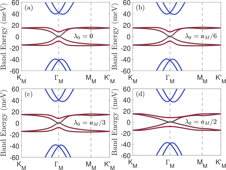
Figure 5: Spectra calculated for different choice of $\psi$ Wannier orbits Eq. (27) at charge neutral point $\nu=4$ and $\Delta_{K}\approx 30$ meV for (a) $\lambda_{0}=0$, (b) $\lambda_{0}=a_{M}/6$, (c) $\lambda_{0}=a_{M}/3$ and (d) $\lambda_{0}=a_{M}/2$. The unit of length is chosen as $a_{M}$ where which is the distance between two nearest AA positions. No obvious change of the spectrum is seen as long as $\lambda_{0}<a_{M}/2$.

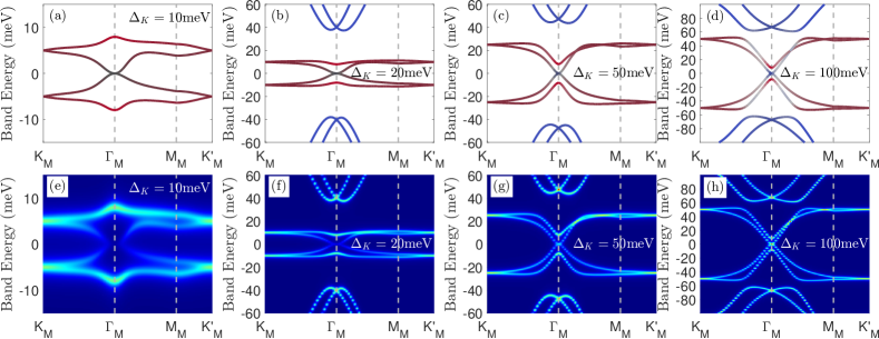
Figure 6: Mott bands calculated by BM model for $\nu=0,\theta=1.14^{\circ},w_{0}/w_{1}=0.8$, with different hybridization strength at (a) $\Delta_{K}=10$ meV, (b) $\Delta_{K}=20$ meV (c) $\Delta_{K}=50$ meV and (d) $\Delta_{K}=100$ meV, where $\Delta_{K}$ is defined as the $K_{M}$ point gap. The blue, red and dark colors of the dispersion line represent the weight of the active band, the remote bands and the ancilla bands, respectively. The corresponding physical electron spectrum function $A_{c}(\mathbf{k},\omega)$ are shown in (e)-(h), with a broading chosen as $\eta=1$ meV.

Figure 7: Mott bands calculated by BM model for $\nu=-1,\theta=1.14^{\circ},w_{0}/w_{1}=0.8$, with different hybridization strength at (a) $\Delta_{K}=10$ meV, (b) $\Delta_{K}=20$ meV and (c) $\Delta_{K}=50$ meV, where $\Delta_{K}$ is defined as the $K_{M}$ point gap. The blue, red and dark colors of the dispersion line represent the weight of the active band, the remote bands and the ancilla bands, respectively. The corresponding physical electron spectrum function $A_{c}(\mathbf{k},\omega)$ are shown in (e)-(g), with a broading chosen as $\eta=1$ meV. (d) shows the $\Gamma_{M}$ point spectrum weight coming from the active, remote and ancilla bands as a function of $\Delta_{K}$. And (h) shows the relative chemical potential shift $\Delta_{\psi}/\Delta_{K}$ as a function of $\Delta_{K}$, which goes to a constant $-1/4$ at large $\Delta_{K}$.

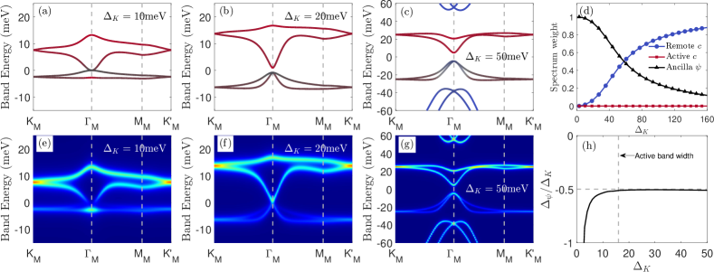
Figure 8: Mott bands calculated by BM model for $\nu=-2,\theta=1.14^{\circ},w_{0}/w_{1}=0.8$, with different hybridization strength at (a) $\Delta_{K}=10$ meV, (b) $\Delta_{K}=20$ meV and (c) $\Delta_{K}=50$ meV, where $\Delta_{K}$ is defined as the $K_{M}$ point gap. The blue, red and dark colors of the dispersion line represent the weight of the active band, the remote bands and the ancilla bands, respectively. The corresponding physical electron spectrum function $A_{c}(\mathbf{k},\omega)$ are shown in (e)-(g), with a broading chosen as $\eta=1$ meV. (d) shows the $\Gamma_{M}$ point spectrum weight coming from the active, remote and ancilla bands as a function of $\Delta_{K}$. And (h) shows the relative chemical potential shift $\Delta_{\psi}/\Delta_{K}$ as a function of $\Delta_{K}$, which goes to a constant $-1/2$ at large $\Delta_{K}$.

To get the hybridization Hamiltonian between the physical layer and the ancilla layer, we can assume the hybridization happens only when the physical electron and its ancilla “copy” coincide at the same lattice in real space, i.e.:

$$H_{0,\mathrm{hyb}}^{(c\psi)}=\Phi_{0}\sum_{l,\mathbf{R},a}c_{0;\mathbf{R},\mathbf{t}_{a},l}^{\dagger}\psi_{0;\mathbf{R},\mathbf{t}_{a},l}+\mathrm{h.c.}~.$$ (29)

Here, $\mathbf{R}$ is the position vector of the original graphene lattice unit cell in layer $l$ and $\mathbf{t}_{a}$ is the relative position vector of sublattice $a$ within a unit cell, $\Phi_{0}$ is the microscopic hybridization strength. One can assume more general hybridization form as long as it respect the symmetry, but the simple form used here is enough to get the essential physics. The hybridization matrix is then projected to the Wannier orbitals of the ancilla layer as:

$$H^{(c\psi)}_{\mathrm{hyb}}= P_{W}^{\psi}H_{0,\mathrm{hyb}}P_{W}^{\psi}$$ (30)

$$= \Phi_{0}\sum_{la\tau s}\sum_{\mathbf{k}\in\mathrm{MBZ},\mathbf{G}_{M}}e^{i\frac{\pi}{4}la}\tilde{W}_{\psi}(\mathbf{k}-\mathbf{K}_{M}^{l}+\mathbf{G}_{M})$$

$$c^{\dagger}_{0,\mathbf{k}+\mathbf{G}_{M};la\tau s}\psi_{\mathbf{k};a\tau s}+\mathrm{h.c.}~,$$

where $P^{\psi}_{W}=\sum_{\mathbf{k}\in\mathrm{MBZ},a\tau s}\psi^{\dagger}_{\mathbf{k};a\tau s}\psi_{\mathbf{k};a\tau s}$ is a projection of $\psi$ to the subspace spanned by the Wannier orbitals $\psi^{\dagger}_{\mathbf{k};a\tau s},\mathbf{k}\in\mathrm{MBZ}$.

In realistic calculation, we can choose a Gaussion like $W_{\psi}(\mathbf{r})$ as in Eq. (27) with a correlation length scale $\lambda_{0}$. In Fig. 5, we show the band structure at $\nu=0$ for several different values of $\lambda_{0}=0,\lambda_{0}=a_{M}/6,\lambda_{0}=a_{M}/3$ and $\lambda_{0}=a_{M}/2$, where $a_{M}$ is the distance between two AA sites. No obvious change of the spectra is seen as long as $\lambda_{0}$ is smaller than $a_{M}/2$, i.e. when two Wannier orbitals has small overlap. We therefore choose a delta-function Wannier orbital and use a constant $\tilde{W}(\mathbf{k})=1$ without otherwise mentioned. In this limit, the hybridization Hamiltonian projected to the ancilla Wannier orbital can be written as:

$$H^{(c\psi)}_{\mathrm{hyb}}=\Phi_{0}\sum_{la\tau s}\sum_{\mathbf{k}\in\mathrm{MBZ},\mathbf{G}_{M}}c^{\dagger}_{0,\mathbf{k}+\mathbf{G}_{M};la\tau s}e^{i\frac{\pi}{4}la}\psi_{\mathbf{k};a\tau s}+\mathrm{h.c.}$$ (31)

Finally, we summarize the total mean-field Hamiltonian model as:

$$H_{\mathrm{MF}}^{(c\psi)}=H_{\mathrm{BM}}+H^{(c\psi)}_{\mathrm{hyb}}-\mu(N_{c}+N_{\psi})+\Delta_{\psi}(N_{\psi}-N_{c})/2~,$$ (32)

with $H_{\mathrm{BM}}$ defined in Eq. (21) and $H_{\mathrm{hyb}}^{(c\psi)}$ defined in Eq. (31). Here we separate the chemical potential defined in the main text Eq. (2) to $\mu=(\mu_{c}+\mu_{\psi})/2$ and $\Delta_{\psi}=\mu_{c}-\mu_{\psi}$.

B.4 Hybridization $\Phi(\mathbf{k})$ projected to the active bands

When $U$ is much smaller than the remote band energy, we can further project the hybridization Hamiltonian into the active flat bands. With knowledge of the symmetries of both the active bands and ancilla bands as listed in Table. 2, we can guess the form of the effective hybridization around the high symmetry points without going through detailed numerical calculations. First, the $C_{2z}T$ symmetry restrict the hybridization Hamiltonian to be

$$H^{(c\psi)}=\sum_{\mathbf{k}\in\mathrm{MBZ}}c_{\mathbf{k}}^{\dagger}\left[\begin{matrix}a(\mathbf{k})&b(\mathbf{k})\\ b^{*}(\mathbf{k})&a^{*}(\mathbf{k})\end{matrix}\right]\psi_{\mathbf{k}}+\mathrm{h.c.}~.$$ (33)

Here we use $c_{\mathbf{k};\pm}$ to denote the active band. If we further consider the approximate chiral symmetry, $b(\mathbf{k})$ can be set to zero, but it can generally have a small value when $w_{0}\neq 0$.

Away from the $\Gamma_{M}$ point, we find that $|a(\mathbf{k})|$ is roughly a constant proportional to the Mott gap. Here we pay a specific attention to the $\Gamma_{M}$ point which can not open a Mott gap due to band topology. At the $\Gamma_{M}$ point where the active bands are $s$ wave orbitals and the ancilla bands are $p_{x}\pm ip_{y}$ wave orbitas, the hybridization matrix is forced to be zero. Around the $\Gamma_{M}$ point, we can choose a gauge such that $\alpha(\mathbf{k})=0$ so that the active bands still transform as an $s$ wave orbital. Then the hybridization Hamiltonian can be linked by a $C_{3z}$ rotation: $a(C_{3z}\mathbf{k})=a(\mathbf{k})e^{i2\pi/3}$, $b(C_{3z}\mathbf{k})=b(\mathbf{k})e^{-i2\pi/3}$, a $C_{2x}$ rotation: $a(C_{2x}\mathbf{k})=a^{*}(\mathbf{k})$, $b(C_{2x}\mathbf{k})=b^{*}(\mathbf{k})$ and a particle-hole transformation : $a(-\mathbf{k})=-a(\mathbf{k}),b(-\mathbf{k})=b(\mathbf{k})$. Expanding the Hamiltonian to the second order of $k=k_{x}+ik_{y}$, a Hamiltonian respecting all the symmetries looks like:

$$H^{(c\psi)}_{\Gamma_{M}}\approx\Phi_{\Gamma_{M}}\sum_{\mathbf{k}}c^{\dagger}_{\mathbf{k}}\left[\begin{matrix}k&\delta k^{2}\\ \delta\bar{k}^{2}&\bar{k}\end{matrix}\right]\psi_{\mathbf{k}},$$ (34)

where $\Phi_{\Gamma_{M}}$ and $\delta$ are parameters which need to be determined numerically.

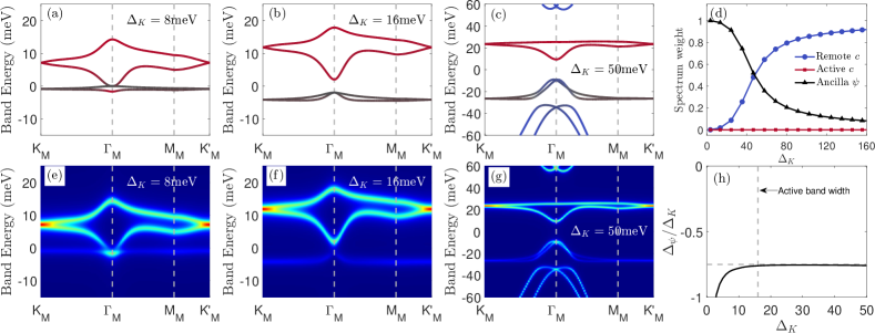
Figure 9: Mott bands calculated by BM model for $\nu=-3,\theta=1.14^{\circ},w_{0}/w_{1}=0.8$, with different hybridization strength at (a) $\Delta_{K}=8$ meV, (b) $\Delta_{K}=16$ meV and (c) $\Delta_{K}=50$ meV, where $\Delta_{K}$ is defined as the $K_{M}$ point gap. The blue, red and dark colors of the dispersion line represent the weight of the active band, the remote bands and the ancilla bands, respectively. The corresponding physical electron spectrum function $A_{c}(\mathbf{k},\omega)$ are shown in (e)-(g), with a broading chosen as $\eta=1$ meV. (d) shows the $\Gamma_{M}$ point spectrum weight coming from the active, remote and ancilla bands as a function of $\Delta_{K}$. And (h) shows the relative chemical potential shift $\Delta_{\psi}/\Delta_{K}$ as a function of $\Delta_{K}$, which goes to a constant $-3/4$ at large $\Delta_{K}$.

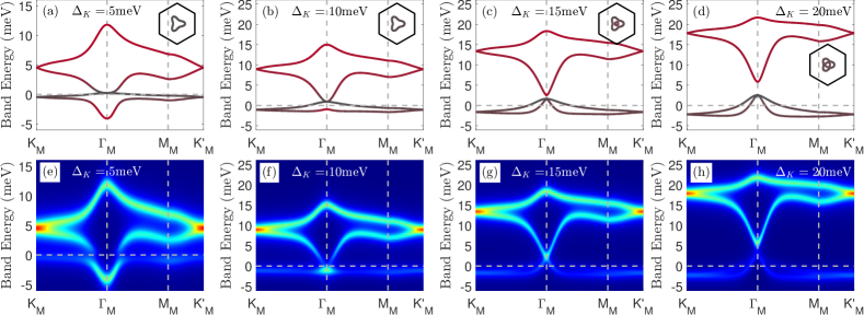
Figure 10: Mott bands calculated by BM model for $\nu=-2-0.4,\theta=1.14^{\circ},w_{0}/w_{1}=0.8$, with different hybridization strength at (a) $\Delta_{K}=5$ meV, (b) $\Delta_{K}=10$ meV (c) $\Delta_{K}=15$ meV and (d) $\Delta_{K}=20$ meV, where $\Delta_{K}$ is defined as the $K_{M}$ point gap. The blue, red and dark colors of the dispersion line represent the weight of the active band, the remote bands and the ancilla bands, respectively. The corresponding Fermi surface are shown in the insets of (a)-(d), where the color of the Fermi surface has the same meaning of the bands. In (e)-(h), we further show the physical electron spectrum function $A_{c}(\mathbf{k},\omega)$ in correspondence with (a)-(d), with a broading chosen as $\eta=1$ meV.

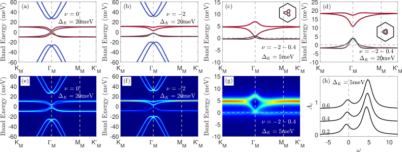
Figure 11: Mott bands calculated by BM model for the magic angle $\theta=1.05^{\circ}$ and $w_{0}/w_{1}=0.8$ for (a) and (e) $\nu=0,\Delta_{K}=20$ meV, (b) and (f) $\nu=-2,\Delta_{K}=20$ meV, and for the doped case (c) and (g) $\nu=-2-0.4,\Delta_{K}=5$ meV and (d) $\nu=-2-0.4,\Delta_{K}=20$ meV, with the Fermi surface shown in the insets of (c) and (d). Again $\Delta_{K}$ is defined as the $K_{M}$ point gap. The colors in the dispersion have the same meaning as in Fig. 2 (a) and the broading is chosen as $\eta=1$ meV. In (h), we show the STM spectrum $A_{c}(\omega)=\sum_{\mathbf{k}}A_{c}(\mathbf{k},\omega)$ for the doped system $\nu=-2-x$, and $x=0.2,0.4,0.6$, with a slightly vertical shift for each $x$.

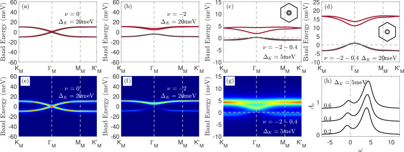
Figure 12: Mott bands calculated by BM model for the magic angle $\theta=1.05^{\circ}$ and chiral limit $w_{0}/w_{1}=0$ for (a) and (e) $\nu=0,\Delta_{K}=20$ meV, (b) and (f) $\nu=-2,\Delta_{K}=20$ meV, and for the doped case (c) and (g) $\nu=-2-0.4,\Delta_{K}=5$ meV and (d) $\nu=-2-0.4,\Delta_{K}=20$ meV, with the Fermi surface shown in the insets of (c) and (d). Again $\Delta_{K}$ is defined as the $K_{M}$ point gap. The colors in the dispersion have the same meaning as in Fig. 2 (a) and the broading is chosen as $\eta=1$ meV. In (h), we show the STM spectrum $A_{c}(\omega)=\sum_{\mathbf{k}}A_{c}(\mathbf{k},\omega)$ for the doped system $\nu=-2-x$, and $x=0.2,0.4,0.6$, with a slightly vertical shift for each $x$.

Writing together the active band $c$ and ancilla band $\psi$ as $\Psi^{\dagger}_{\mathbf{k}}=(c_{\mathbf{k};+}^{\dagger},\psi_{\mathbf{k};+}^{\dagger},c_{\mathbf{k};-}^{\dagger},\psi_{\mathbf{k};-}^{\dagger})$ and keep only the linear terms, the full low-energy Hamiltonian near the $\Gamma_{M}$ point then takes the following form:

$$H_{\Psi}= \sum_{\mathbf{k}}\Psi^{\dagger}_{\mathbf{k}}\left[\begin{matrix}-\Delta_{\psi}/2&\Phi_{\Gamma_{M}}k&M&0\\ \Phi_{\Gamma_{M}}\bar{k}&\Delta_{\psi}/2&0&0\\ M&0&-\Delta_{\psi}/2&\Phi_{\Gamma_{M}}\bar{k}\\ 0&0&\Phi_{\Gamma_{M}}k&\Delta_{\psi}/2\\ \end{matrix}\right]\Psi_{\mathbf{k}}$$ (35)

$$-\mu\sum_{\mathbf{k}}\Psi^{\dagger}_{\mathbf{k}}\Psi_{\mathbf{k}}~,$$

which can be seen as an AB stacking graphene model at the $K$ point, with $c_{+}$ and $\psi_{+}$ forming the first layer and $c_{-}$, $\psi_{-}$ forming the second layer.

At $\nu=0$, we have $\Delta_{\psi}=\mu=0$ and thus we can easily get the Hubbard bands around the $\Gamma$ point to be:

$$\epsilon_{k}=\pm M/2\pm\sqrt{(M/2)^{2}+|\Phi_{\Gamma_{M}}\mathbf{k}|^{2}}\approx\left\{\begin{aligned} &\pm M\\ &\pm|\Phi_{\Gamma_{M}}k|^{2}/M\end{aligned}\right.~.$$ (36)

Appendix C Results from ancilla theory in continuum model

In this appendix we show more results of the charge sector in ancilla theory based on the continuum model Eq. (32). We show the Mott bands for the integer filings $\nu=0,-1,-2,-3$, the doped case $\nu=-2-x$, and the results for the magic angle $\theta=1.05^{\circ}$ and chiral limit $w_{0}/w_{1}=0$. For all of the results, we use the $K_{M}$ point band gap $\Delta_{K}$ (instead of the microscopic parameter $\Phi_{0}$ in Eq. (31)) to characterize the Mott gap size, which has similar physical meaning with the $\Delta_{\mathrm{Mott}}$ defined in Eq. (11) in Appendix. A for conventional Hubbard model. Note also that we always define $\Delta_{K}$ as the band gap between two lowest $p$-wave orbital when band crossing happens, as the $s$-wave orbital has zero overlap with the $\psi$ orbital and does not contribute to the Mott physics.

C.1 Integer fillings

We plot the Mott bands and physical spectral functions $A_{c}(\mathbf{k},\omega)$ for integer fillings $\nu=0$ in Fig. 6, $\nu=-1$ in Fig. 7, $\nu=-2$ in Fig. 8 and $\nu=-3$ in Fig. 9. The $\nu>0$ results are not shown here due to the particle-hole symmetry of our model.

For the charge neutrality point, we show the semi-metal bands for more interaction strength $\Delta_{K}=10$ meV, $20$ meV, $50$ meV and $100$ meV. The $\Gamma_{M}$ point remain gapless regardless of the Mott interaction $\Delta_{K}$. The $\Gamma_{M}$ effective mass decreases and remote band weight increases as $\Delta_{K}$ increases, consistent with our conclusion in the main text.

For other integer filling, both the $\nu=-1$ and $\nu=-3$ case goes through a semi-metal to insulator transition as the interaction $\Delta_{K}$ is gradually increased, similar to the $\nu=-2$ results. The gapless mode at $\Gamma_{M}$ point in semi-metal phase is mainly contributed by $\psi$ band and is almost invisible in the spectrum function. Upon increasing $\Delta_{K}$, the $\Gamma_{M}$ point spectrum weight gradually increases when the remote bands comes in. The main difference for different integer fillings is that the $\Gamma_{M}$ point gap is much weaker for $\nu=-1$ and much stronger for $\nu=-3$, as also shown in Fig. 3 (d) in the main text. We therefore expect a more robust semi-metal phase for $\nu=-1$.

As discussed in the main text, the gap at $\Gamma_{M}$ point is not directly from the Mott interaction $U$, but from a Chemical potential shift of the ancilla and active band $\Delta_{\psi}$. Here we plot $\Delta_{\psi}/\Delta_{K}$ as a function of $\Delta_{K}$ for different dopings in Fig. 7 (h), Fig. 8 (h) and Fig. 9 (h). When the Mott gap $\Delta_{K}$ is larger than the active bandwidth $2M$, the chemical potential shift $\Delta_{\psi}$ satisfies the relation $\Delta_{\psi}=\nu\Delta_{K}/4$ for all the integer fillings $\nu=-1,-2,-3$. On the other hand, the above relation fails in the semi-metal phase when $\Delta_{K}$ is comparable with $2M$.

C.2 Pseudogap metal at $\nu=-2-x$

More results of the pseudogap metal are shown in Fig. 10 for $\nu=-2-0.4$. Similar to the main text results Fig. 4, the Fermi surface are mainly contributed by the ancilla layer $\psi$, which almost disappear in the physical electron spectrum $A_{c}(\mathbf{k},\omega)$. A transition from single Fermi surface to two Fermi surfaces happens between $\Delta_{K}=10$ meV and $\Delta_{K}=15$ meV, which is in correspondence with the semi-metal to insulator transition at inter filling $\nu=-2$.

C.3 Magic angle and chiral limit

Finally, we briefly show the results of magic angle $\theta=1.05^{\circ},w_{0}/w_{1}=0.8$ in Fig. 11 and the chiral limit $\theta=1.05^{\circ},w_{0}/w_{1}=0$ in Fig. 12. Overall, the results are similar to our main results in $\theta=1.14^{\circ},w_{0}/w_{1}=0.8$ case, but the semi-metal phase shrinks due to the narrower bandwidth of the active bands. Specifically, the two lower Hubbard bands at $\nu=-2$ and $\nu=-2-x$ coincide with each other in the chiral limit $w_{0}/w_{1}=0$ in Figs. 12 (c) and (d). And the double peaks on the positive bias side in Fig. 4 (e) becomes a single one in Fig. 11 (h) and Fig. 12 (h) due to a narrower bandwidth.

	$C_{2z}T$	$P$	$S$	$C_{3z}$	$C_{2x}$
$c_{1,\mathbf{k}}$	$\sigma_{x}\mathcal{K}c_{1,\mathbf{k}}$	$-\mathrm{i}\sigma_{z}\mathcal{K}c^{\dagger}_{1,-\mathbf{k}}$	$-\sigma_{z}\mathcal{K}c_{1,\mathbf{k}}$	$e^{\mathrm{i}2\pi/3\sigma_{z}}c_{1,C_{3z}\mathbf{k}}$	$\sigma_{x}c_{1,C_{2x}\mathbf{k}}$
$c_{2,\mathbf{k}}$	$\sigma_{x}\mathcal{K}c_{2,\mathbf{k}}$	$-\mathrm{i}\sigma_{z}\mathcal{K}c^{\dagger}_{2,-\mathbf{k}}$	$\sigma_{z}\mathcal{K}c_{2,\mathbf{k}}$	$\sigma_{0}c_{2,C_{3z}\mathbf{k}}$	$\sigma_{x}c_{2,C_{2x}\mathbf{k}}$
$f_{\mathbf{k}}$	$\sigma_{x}\mathcal{K}f_{\mathbf{k}}$	$\mathrm{i}\sigma_{z}\mathcal{K}f^{\dagger}_{-\mathbf{k}}$	$\sigma_{z}\mathcal{K}f_{\mathbf{k}}$	$e^{\mathrm{i}2\pi/3\sigma_{z}}f_{C_{3z}\mathbf{k}}$	$\sigma_{x}f_{C_{2x}\mathbf{k}}$
$\psi_{\mathbf{k}}$	$\sigma_{x}\mathcal{K}\psi_{\mathbf{k}}$	i$\sigma_{z}\mathcal{K}\psi^{\dagger}_{-\mathbf{k}}$	$\sigma_{z}\mathcal{K}\psi_{\mathbf{k}}$	$e^{\mathrm{i}2\pi/3\sigma_{z}}\psi_{C_{3z}\mathbf{k}}$	$\sigma_{x}\psi_{C_{2x}\mathbf{k}}$

Table 3: Symmetry action on $c,f,\psi$ fermion.

Appendix D Ancilla theory in the topological heavy fermion model

Here we review the topological heavy fermion model [32] and the detail of its symmetry transformation. The THFM contains heavy fermion $f$ and two types of itinerant electrons $c_{1},c_{2}$. The free Hamiltonian of THFM is written as:

$$\begin{split}H_{\mathrm{THFM}}=&\sum_{\mathbf{k},\tau,s}\left(v_{\star}\left(\tau k_{x}\sigma_{0}+\mathrm{i}k_{y}\sigma_{z}\right)c^{\dagger}_{1,\mathbf{k};\tau s}c_{2,\mathbf{k};\tau s}+\mathrm{H.c.}\right)\\ &+\sum_{\mathbf{k},\tau,s}c^{\dagger}_{2,\mathbf{k};\tau s}M\sigma_{x}c_{2,\mathbf{k};\tau s}+H^{\left(cf\right)}_{0},\\ H^{(cf)}_{0}=&\frac{1}{\sqrt{N_{\mathrm{site}}}}\sum_{\mathbf{k},i,\tau,s}\Big{(}e^{\mathrm{i}\mathbf{k}\cdot\mathbf{R}_{i}-\frac{k^{2}\lambda^{2}}{2}}f^{\dagger}_{i;\eta s}\big{(}\gamma\sigma_{0}\\ &+v^{\prime}_{\star}\left(k_{x}\sigma_{x}+k_{y}\sigma_{y}\right)\big{)}c_{1,\mathbf{k};\tau s}+\mathrm{H.c.}\Big{)}.\end{split}$$ (37)

In our calculation, we choose that $\theta=1.14^{\circ}$, $v_{\star}=-4.544$ eV $\overset{\circ}{A}$, $M=-7.422$ meV, $\gamma=-38.037$ meV, $v^{\prime}_{\star}=1.702$ eV $\overset{\circ}{A}$, $\lambda=0.3375a_{M}$. Here $i$ represents the AA sites of TBG and $\mathbf{k}$ is summed over the entire momentum space. $f_{i;\tau s}=(f_{i;+\tau s},f_{i;-\tau s})^{T}$, $c_{1;\tau s}(\mathbf{k})=(c_{1;+\tau s}(\mathbf{k}),c_{1;-\tau s}(\mathbf{k}))^{T}$, $c_{2;\tau s}(\mathbf{k})=(c_{2;+\tau s}(\mathbf{k}),c_{2;-\tau s}(\mathbf{k}))^{T}$. $\sigma$ represents the Pauli matrix in orbital space. The symmetry action of $f,c_{1},c_{2}$ are listed in Table. 3. The first ancilla fermion $\psi$ stays in the same orbital with $f$, hence they transform in the same way under symmetry action. $f$ and $\psi$ are coupled as:

$$H_{\mathrm{hyb}}=\Phi\sum_{i,a,\tau,s}\left(f^{\dagger}_{i;a\tau s}\psi_{i;a\tau s}+\mathrm{H.c.}\right).$$ (38)

The total Hamiltonian can be written as:

$$\begin{split}H^{(cf\psi)}_{\mathrm{MF}}=&H_{\mathrm{THFM}}+H_{\mathrm{hyb}}-\mu(N_{c_{1}}+N_{c2}+N_{f})\\ &-\mu_{\psi}N_{\psi},\end{split}$$ (39)

which is Eq. 4 in the main text.

D.1 Effective model at $\nu=0$

For $\nu=0$ and in the limit $\gamma\gg M,\Phi$, $c$ and $f_{1}$ are gapped. The low energy part of Eq. (39) only contains $c_{2}$ and $\psi$. The effective model can be written as:

$$\begin{split}H^{(c_{2}f)}_{\mathrm{eff}}\approx&\frac{\Phi v_{\star}}{\sqrt{2}\gamma}\sum_{\mathbf{k},\tau,s}\left(c^{\dagger}_{2,\mathbf{k};\tau s}\begin{bmatrix}-k&\frac{v^{\prime}_{\star}}{\gamma}k^{2}\\ \frac{v^{\prime}_{\star}}{\gamma}\bar{k}^{2}&-\bar{k}\end{bmatrix}\psi_{\mathbf{k};\tau s}+\mathrm{H.c.}\right)\\ &+\sum_{\mathbf{k},\tau,s}c^{\dagger}_{2,\mathbf{k};\tau s}M\sigma_{x}c_{2,\mathbf{k};\tau s},\end{split}$$ (40)

where $k=k_{x}+\mathrm{i}k_{y}$. This equation is consistent with the result in BM model Eq. (34).

D.2 Comparison with the calculation in BM model

We present the Mott bands and physical spectral functions $A_{c}(\omega,\mathbf{k})$ for integer fillings $\nu=0$ in Fig. 13, $\nu=-1$ in Fig. 14, $\nu=-2$ in Fig. 15, $\nu=-3$ in Fig. 16, for pseudogap metal at $\nu=-2-0.4$ in Fig. 17, for the magic angle and chiral limit case in Fig. 18,  19. The results are similar to that from the BM model Fig. 6$-$ 12. This indicates that the ancilla theory is basis independent and we can obtain consistent results from different single particle basis.

Figure 13: Mott bands calculated by THFM for $\theta=1.14^{\circ},\nu=0$ with different hybridization strength at (a) $\Delta_{K}=10$ meV, (b) $\Delta_{K}=20$ meV and (c) $\Delta_{K}=50$ meV and (d) $\Delta_{K}=100$ meV. The colors has the same meaning as in Figs. 2 (a) and (b). The corresponding physical electron spectrum function $A_{c}(\mathbf{k},\omega)$ are shown in (e)-(h).

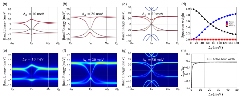
Figure 14: Mott band calculated by THFM for $\theta=1.14^{\circ},\nu=-1$ with different hybridization strength at (a) $\Delta_{K}=10$ meV, (b) $\Delta_{K}=20$ meV and (c) $\Delta_{K}=50$ meV. The colors has the same meaning as in Figs. 2 (a) and (b). The corresponding physical electron spectrum function $A_{c}(\mathbf{k},\omega)$ are shown in (e)-(g). (d) shows the $\Gamma_{M}$ point spectrum weight coming from the active, remote and ancilla bands as a function of $\Delta_{K}$. And (h) shows the relative chemical potential shift $\Delta_{\psi}/\Delta_{K}$ as a function of $\Delta_{K}$, which goes to a constant $-1/4$ at large $\Delta_{K}$.

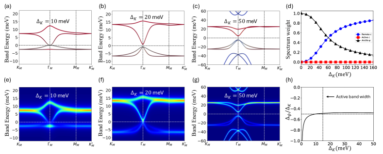
Figure 15: Mott bands calculated by THFM for $\theta=1.14^{\circ},\nu=-2$ with different hybridization strength at (a) $\Delta_{K}=10$ meV, (b) $\Delta_{K}=20$ meV and (c) $\Delta_{K}=50$ meV. The colors has the same meaning as in Figs. 2 (a) and (b). The corresponding physical electron spectrum function $A_{c}(\mathbf{k},\omega)$ are shown in (e)-(g). (d) shows the $\Gamma_{M}$ point spectrum weight coming from the active, remote and ancilla bands as a function of $\Delta_{K}$. And (h) shows the relative chemical potential shift $\Delta_{\psi}/\Delta_{K}$ as a function of $\Delta_{K}$, which goes to a constant $-1/2$ at large $\Delta_{K}$.

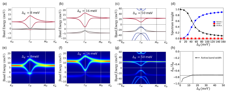
Figure 16: Mott bands calculated by THFM for $\theta=1.14^{\circ},\nu=-3$ with different hybridization strength at (a) $\Delta_{K}=8$ meV, (b) $\Delta_{K}=16$ meV and (c) $\Delta_{K}=50$ meV. The colors has the same meaning as in Figs. 2 (a) and (b). The corresponding physical electron spectrum function $A_{c}(\mathbf{k},\omega)$ are shown in (e)-(g). (d) shows the $\Gamma_{M}$ point spectrum weight coming from the active, remote and ancilla bands as a function of $\Delta_{K}$. And (h) shows the relative chemical potential shift $\Delta_{\psi}/\Delta_{K}$ as a function of $\Delta_{K}$, which goes to a constant $-3/4$ at large $\Delta_{K}$.

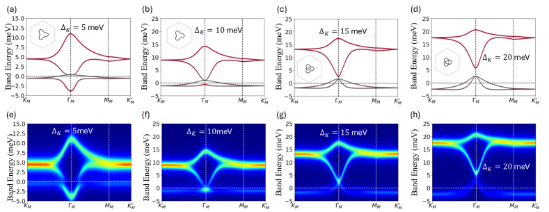
Figure 17: Mott bands calculated by THFM model for $\theta=1.14^{\circ},\nu=-2-0.4$, with different hybridization strength at (a) $\Delta_{K}=5$ meV, (b) $\Delta_{K}=10$ meV (c) $\Delta_{K}=15$ meV and (d) $\Delta_{k}=20$ meV, where $\Delta_{K}$ is defined as the $K_{M}$ point gap. The blue, red and dark colors of the dispersion line represent the weight of the active band, the remote bands and the ancilla bands, respectively. The corresponding Fermi surface are shown in the insets of (a)-(d). In (e)-(h), we further show the physical electron spectrum function $A_{c}(\mathbf{k},\omega)$ in correspondence with (a)-(d), with a broading chosen as $\eta=1$ meV.

Figure 18: Mott bands calculated by THFM model for the magic angle $\theta=1.05^{\circ}$ for (a) and (e) $\nu=0,\Delta_{K}=20$ meV, (b) and (f) $\nu=-2,\Delta_{K}=20$ meV, and for the doped case (c) and (g) $\nu=-2-0.4,\Delta_{K}=5$ meV and (d) $\nu=-2-0.4,\Delta_{K}=20$ meV, with the Fermi surface shown in the insets of (c) and (d). Again $\Delta_{K}$ is defined as the $K_{M}$ point gap. The broading is chosen as $\eta=1$ meV. In (h), we show the STM spectrum $A_{c}(\omega)=\sum_{\mathbf{k}}A_{c}(\mathbf{k},\omega)$ for the doped system $\nu=-2-x$, and $x=0.2,0.4,0.6$, with a slightly vertical shift for each $x$. In this calculation, we choose that $v_{\star}=-4.303$ eV $\overset{\circ}{A}$, $M=3.697$ meV, $\gamma=-24.75$ meV, $v^{\prime}_{\star}=1.622$ eV $\overset{\circ}{A}$, $\lambda=0.3375a_{M}$.

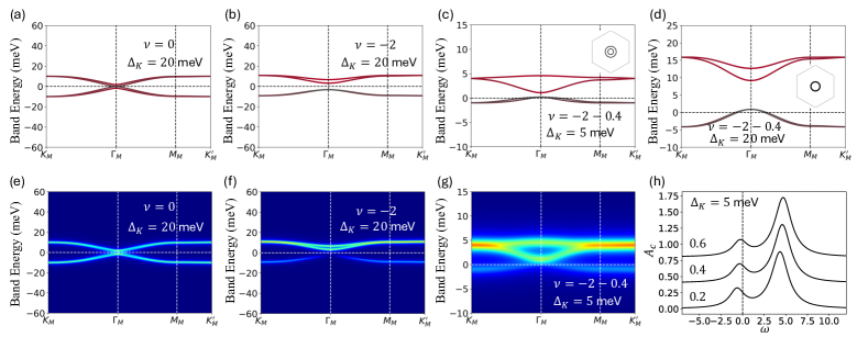
Figure 19: Mott bands calculated by THFM model for the magic angle $\theta=1.05^{\circ}$ in the chiral limit for (a) and (e) $\nu=0,\Delta_{K}=20$ meV, (b) and (f) $\nu=-2,\Delta_{K}=20$ meV, and for the doped case (c) and (g) $\nu=-2-0.4,\Delta_{K}=5$ meV and (d) $\nu=-2-0.4,\Delta_{K}=20$ meV, with the Fermi surface shown in the insets of (c) and (d). Again $\Delta_{K}$ is defined as the $K_{M}$ point gap. The broading is chosen as $\eta=1$ meV. In (h), we show the STM spectrum $A_{c}(\omega)=\sum_{\mathbf{k}}A_{c}(\mathbf{k},\omega)$ for the doped system $\nu=-2-x$, and $x=0.2,0.4,0.6$, with a slightly vertical shift for each $x$. In this calculation, we choose that $v_{\star}=-5.144$ eV $\overset{\circ}{A}$, $M=3.697$ meV, $\gamma=-100.79$ meV, $v^{\prime}_{\star}=0$, $\lambda=0.3375a_{M}$.

Appendix E Correlated insulator to semimetal transition in $U\gg\gamma$ limit of THFM

In the main text we discussed a semimetal to insulator transition at filling $\nu=-1,-2,-3$ by increasing $U$ in the regime $U<\gamma$ or $U\sim\gamma$. It turns out that there is a similar transition in the $U\gg\gamma$ limit, where the THFM offers a good starting point. Here we will discuss this transition based on simple $\frac{\gamma^{2}}{U}$ perturbation in THFM and show that the result matches the calculation in the ancilla theory. This supports the correctness of the ancilla theory in the $U\gg\gamma$ limit.

E.1 $\frac{\gamma^{2}}{U}$ perturbation theory in THFM

In the THFM, the total Hamiltonian can be written as:

$$H=H_{0}+\frac{U}{2}\sum_{i}\left(n_{f,i}-4\right)^{2}-\mu_{f}N_{f},$$ (41)

where $H_{0}$ is the free term and $i$ represents AA sites. $\frac{U}{2}\left(n_{f,i}-4\right)^{2}$ is the $SU(8)$ Hubbard interaction of $f$ electrons. $\mu_{f}$ is tuned to fix $f$ electrons at integer filling $4+\nu$. If we only consider $c$ electrons at $\Gamma$ point, $H_{0}$ can be simplified as:

$$H_{0}(\Gamma)=\frac{\gamma}{\sqrt{N_{\mathrm{site}}}}\sum_{i,a,\tau,s}(c^{\dagger}_{1,\Gamma;a\tau s}f_{i;a\tau s}+\mathrm{H.c.}),$$ (42)

At integer filling $\nu$, we now perform a perturbation calculation to the order $o(\frac{\gamma^{2}}{U})$ in the large $U\gg\gamma$ limit. We assume $f$ orbital is Mott localized with total filling $n_{f}=4+\nu$. The contributions come from two kinds of processes: (1) $c_{1}\rightarrow f,f\rightarrow c_{1}$; (2) $f\rightarrow c_{1},c_{1}\rightarrow f$. The total contribution can be written as:

$$\begin{split}&-\frac{1}{N_{\mathrm{site}}}\sum_{i,a,\tau,s}\big{(}J_{K;1}c^{\dagger}_{1,\Gamma;a\tau s}f_{i;a\tau s}f^{\dagger}_{i;a^{\prime}\tau^{\prime}s^{\prime}}c_{1,\Gamma;a^{\prime}\tau^{\prime}s^{\prime}}\\ &+J_{K;2}f^{\dagger}_{i;a\tau s}c_{1,\Gamma;a\tau s}c^{\dagger}_{1,\Gamma;a^{\prime}\tau^{\prime}s^{\prime}}f_{i;a^{\prime}\tau^{\prime}s^{\prime}}\big{)}\\ =&\frac{J_{K;1}+J_{K;2}}{N_{\mathrm{site}}}\sum_{i}\left(\sum_{\alpha,\beta}S_{c_{1},\Gamma;\alpha\beta}S_{f,i;\beta\alpha}+\frac{n_{c_{1},\Gamma}n_{f,i}}{8}\right)\\ &-\left(J_{K;1}n_{c_{1},\Gamma}+\frac{J_{K;2}}{N_{\mathrm{site}}}\sum_{i}n_{f,i}\right),\end{split}$$ (43)

where $J_{K;1}=\frac{\gamma^{2}}{U/2-\mu_{f}+\nu U}$ and $J_{k;2}=\frac{\gamma^{2}}{U/2+\mu_{f}-\nu U}$. $S_{c_{1},\Gamma;\alpha\beta}=c^{\dagger}_{1,\Gamma;\alpha}c_{1,\Gamma;\beta}-\frac{1}{8}n_{c_{1},\Gamma}$, $S_{f,i;\alpha\beta}=f^{\dagger}_{i;\alpha}f_{i;\beta}-\frac{\delta_{\alpha\beta}}{8}n_{f,i}$, where $\alpha,\beta=a\tau s$.

The effective Hamiltonian consists of a $SU(8)$ Kondo coupling between $c$ electron and the localized spin moments from $f$ orbital. But there is an additional energy shift for the $c_{1}$ state due to the virtual process. In the absence of any sublattice/valley/spin order of the local $f$ spin moments, the energy shift of $c_{1}$ can be estimated as:

$$\begin{split}&\frac{J_{K;1}+J_{K;2}}{8}\left(n_{c_{1},\Gamma}-\frac{8J_{K;2}}{J_{K;1}+J_{K;2}}\right)\\ &\left(\frac{1}{N_{\mathrm{site}}}\sum_{i}n_{f,i}-\frac{8J_{K;1}}{J_{K;1}+J_{K;2}}\right)+\mathrm{Const.},\end{split}$$ (44)

which contributes an energy shift to $c_{1}$ electrons at $\Gamma$ point. By substituting $J_{K;1}=\frac{\gamma^{2}}{U/2-\mu_{f}+\nu U}$ and $J_{K;2}=\frac{\gamma^{2}}{U/2+\mu_{f}-\nu U}$ into the above equation, we can obtain the shift term as:

$$\frac{\gamma^{2}\left(\nu U-8(\mu_{f}-\nu U)\right)}{2\left(U^{2}-4(\mu_{f}-\nu U)^{2}\right)}n_{c_{1},\Gamma}.$$ (45)

In the following we set $\mu_{f}=\nu U$. At $\nu=0$, the energy shift vanishes. This is also ensured by the particle hole symmetry at charge neutrality. At other integer fillings $\nu=\pm 1,\pm 2,\pm 3$, The energy shift is $\frac{\gamma^{2}\nu}{2U}$ for $c_{1}$.

$c_{1}$ and $c_{2}$ are kept at charge neutrality together. But now there is an energy shift for $c_{1}$, but not for $c_{2}$. Therefore, $c$ bands at $\Gamma$ point have four energies: $\{\frac{\gamma^{2}\nu}{2U},\frac{\gamma^{2}\nu}{2U},\pm M\}$. Here the first two energies correspond to $c_{1}$ electrons and the rest corresponds to $c_{2}$ electrons. When the $c$ electrons are half filling, the gap of the Hubbard bands at integer filling $\nu$ can be estimated as:

$$\Delta_{\Gamma}=\left\{\begin{array}[]{rcl}&\left|\left|\frac{\gamma^{2}\nu}{2U}\right|-\left|M\right|\right|&\left|\frac{\gamma^{2}\nu}{2U}\right|>\left|M\right|\\ &0&\left|\frac{\gamma^{2}\nu}{2U}\right|<\left|M\right|\end{array}\right.$$ (46)

One can see that there is a semimetal to insulator transition by reducing $U$ in the $U\gg\gamma$ limit. Its nature is actually quite similar to the transition at $U<\gamma$ limit presented in the main text. Just in the later case the $c_{1},c_{2},f$ basis is not a good staring point, as the semimetal is formed by the active band $c_{\mathbf{k}}$ and ancilla $\psi_{\mathbf{k}}$. But it is still interesting to see a one to one correspondence between the emergent $c,\psi$ bands and the single particle $c_{1},c_{2}$ bands in the $U\gg\gamma$ limit. In the $U\gg\gamma$ limit, we also find a Kondo coupling between $c_{1}$ and the local $f$ moments. In the $U<\gamma$ limit, we believe there is also an effective Kondo coupling between the emergent $\psi$ band and the local moments in $\psi^{\prime}$ layer. In this work we assume the spin moments in $\psi^{\prime}$ layer are easier thermally fluctuating at finite $T$ or are quenched by an anti-Hund’s coupling $J_{A}$ at $T=0$, so we can ignore the Kondo coupling. We can imagine that the effective Kondo coupling may be important to understand symmetry breaking (ferromagnetic phases) and superconductor phase, which we will investigate in a future work.

E.2 Benchmark in the ancilla theory

The above perturbation calculation only applies for $U\gg\gamma$ limit. Our ancilla theory should work in the whole range of $U$. Here we demonstrate that the same result can be obtained in the $U\gg\gamma$ limit of the ancilla theory.

In the presence of ancilla fermion $\psi$, the mean field Hamiltonian of the charge sector is:

$$\begin{split}H=&H_{0}+\Phi\sum_{\mathbf{k},a,\tau,s}\left(f^{\dagger}_{\mathbf{k};a\tau s}\psi_{\mathbf{k};a\tau s}+\mathrm{H.c.}\right)\\ &+\frac{\Delta_{\psi}}{2}(N_{\psi}-N_{f})-\mu(N_{f}+N_{\psi}),\end{split}$$ (47)

where $\mathbf{k}\in\mathrm{MBZ}$ and $N_{\psi}$ is the total density operator of $\psi$ electrons, $\Delta_{\psi}$ is tuned to fix $\frac{1}{N_{\mathrm{site}}}\langle N_{\psi}\rangle=4-\nu$. In the large $\Phi$ limit, the dominant term of Eq. (47) is $\Phi\sum_{\mathbf{k},\alpha,\eta,s}\left(f^{\dagger}_{\alpha\eta s}(\mathbf{k})\psi_{\alpha\eta s}(\mathbf{k})+\mathrm{H.c.}\right)$, $\frac{\Delta_{\psi}}{2}(N_{\psi}-N_{f})$ and $\mu_{(}N_{f}+N_{\psi})$. Hence the density $\langle N_{\psi}\rangle$ can be calculated as:

$$\langle N_{\psi}\rangle=8N_{\mathrm{site}}\frac{\left(-\Delta_{\psi}/2+\sqrt{\Phi^{2}+\Delta_{\psi}^{2}/4}\right)^{2}}{\Phi^{2}+\left(-\Delta_{\psi}/2+\sqrt{\Phi^{2}+\Delta_{\psi}^{2}/4}\right)^{2}}.$$ (48)

By solving $\langle N_{\psi}\rangle=N_{\mathrm{site}}(4-\nu)$, we can obtain:

$$\Delta_{\psi}=\frac{2\nu}{\sqrt{16-\nu^{2}}}\Phi.$$ (49)

If we use the notation of $\Delta_{\mathrm{Mott}}=2\sqrt{\Phi^{2}+\frac{\Delta_{\psi}^{2}}{4}}$, we find $\Delta_{\psi}=\frac{\nu}{4}\Delta_{\mathrm{Mott}}$ as found in Appendix. A.

Then we can include $c_{1}$ electrons at $\Gamma$ point to estimate the energy shift of $c_{1}$ electrons. The free term is still Eq. (42). Then the Hamiltonian of $c_{1},f,\psi$ can be represented as:

$$\sum_{a,\tau,s}\begin{pmatrix}c^{\dagger}_{1,\Gamma;a\tau s}&f^{\dagger}_{\Gamma;a\tau s}&\psi^{\dagger}_{\Gamma;a\tau s}\end{pmatrix}h\begin{pmatrix}c_{1,\Gamma;a\tau s}\\ f_{\Gamma;a\tau s}\\ \psi_{\Gamma;a\tau s}\end{pmatrix},$$ (50)

where $h$ is:

$$\begin{bmatrix}0&\gamma&0\\ \gamma&·-\frac{\Delta_{\psi}}{2}-\mu&\Phi\\ 0&\Phi&\frac{\Delta_{\psi}}{2}-\mu\end{bmatrix}.$$ (51)

And then by simply second order perturbation theory, we can get the energy shift for $c_{1}$ band as:

$$\delta E_{c_{1}}=\frac{\nu\Delta_{\mathrm{Mott}}-8\mu}{2\left(\Delta_{\mathrm{Mott}}^{2}-4\mu^{2}\right)}.$$ (52)

The result agrees with that from the $\gamma^{2}/U$ perturbation calculation if we set $\Delta_{\mathrm{Mott}}=U,\mu=\mu_{f}-\nu U$. If we choose $\mu=0$, then there is:

$$\delta E_{c_{1}}=\frac{\gamma^{2}\nu}{2\Delta_{\mathrm{Mott}}}.$$ (53)

Appendix F Physical meaning of the ancilla fermion

We have seen that the lower Hubbard band at $\nu=-2$ is dominated by the ancilla fermion $\psi$ and the small Fermi surface at $\nu=-2-x$ is formed by $\psi$. Here we show that the ancilla fermion $\psi$ represents a many-body excitation and should be interpreted as a composite polaron close to $\mathbf{k}=0$. Suppose we have a many body ground state $\ket{G_{c}}=P_{s}\ket{G_{0}}$, where $\ket{G_{0}}$ is the state in the enlarged Hilbert space with $c,\psi,\psi^{\prime}$, $\psi_{\mathbf{k}}$ can be related to a physical operator $O_{\mathbf{k}}$ from the equation $P_{S}\psi_{\mathbf{k};\alpha}\ket{G_{0}}=O_{\mathbf{k};\alpha}P_{S}\ket{G_{0}}$. It is easy to see that $O_{\mathbf{k}}$ has the same quantum number as $\psi_{k}$, but may be a complicated composite operator, which actually depends on the many body state $\ket{G_{c}}=P_{S}\ket{G_{0}}$. Let us restricted to the active bands. Simply from symmetry, we can expand $O_{\mathbf{k}}$ in the form:

$$O_{\mathbf{k};\alpha}=\sqrt{Z_{\mathbf{k}}}c_{\mathbf{k};\alpha}+\sum_{\mathbf{k}^{\prime},\mathbf{q}}F(\mathbf{k}^{\prime},\mathbf{q})c_{\mathbf{k}+\mathbf{q};\beta}c^{\dagger}_{\mathbf{k}^{\prime}+\mathbf{q};\beta}c_{\mathbf{k};\alpha^{\prime}}+...$$ (54)

Here $\alpha,\beta$ is the SU(8) flavor index. When $\mathbf{k}=0$, $Z_{\mathbf{k}}=0$ because of $C_{3z}$ symmetry. Then the leading order of $O_{\mathbf{k};\alpha}$ is a composite polaron or composite trion operator. Because most of the states in $\bf k$ space is from the $f$ band in THMF, we can expand $O_{\mathbf{k}}$ in terms of $f$ orbital as:

$$O_{\mathbf{k};\alpha} =A_{\bf k}P_{0}\frac{1}{\sqrt{N_{\mathrm{site}}}}\sum_{i}f_{i;\alpha}e^{-i\mathbf{k}\cdot\mathbf{R}_{i}}P_{0}$$

$$~~~+B_{\mathbf{k}}P_{0}\frac{1}{\sqrt{N_{\mathrm{site}}}}\sum_{i}\sum_{\delta}f_{i+\delta;\beta}S^{f}_{i;\beta\alpha}e^{-i\bf k\cdot\mathbf{R}_{i}}P_{0}+...$$ (55)

where $S^{f}_{i;\beta\alpha}=f^{\dagger}_{i;\beta}f_{i;\alpha}$ is a spin operator on AA site $i$. $P_{0}$ is the projection operator to the active bands. $i+\delta$ labels the nearest neighbor site of $i$. Note the first term just gives $f_{\mathbf{k};\alpha}$, which after projection $P_{0}$ is zero for $\mathbf{k}=0$. Thus for $\bf k=0$, $O_{\mathbf{k}}$ is dominated by the second term and represents a polaron with spin on AA site and the hole on the nearest neighbor AA site. In terms of the active band electron operator, close to $\bf k=0$, $O_{\mathbf{k}}$ is in the form:

$$O_{\mathbf{k};\alpha}\sim\frac{1}{N_{\mathrm{site}}}\sum_{\mathbf{k}^{\prime},\mathbf{q}}F_{\beta\beta\alpha}(\mathbf{k}^{\prime},\mathbf{q})c_{\beta;\mathbf{k}+\mathbf{q}}c^{\dagger}_{\beta;\mathbf{k}^{\prime}+\mathbf{q}}c_{\mathbf{k};\alpha^{\prime}}$$ (56)

where $F_{\beta\beta\alpha}(\mathbf{k},\mathbf{q})=\left(\sum_{\delta}e^{i\mathbf{k}\cdot\mathbf{\delta}}\right)\mu_{f;\beta}(\mathbf{k}+\mathbf{q})\mu_{f;\alpha}(\mathbf{k}^{\prime})\mu_{f;\beta}^{*}(\mathbf{k}^{\prime}+\mathbf{q})$, $\mu_{f;\alpha}(\bf k)$ is the $f$ component of the Bloch wavefunction of the active band in the flavor $\alpha$. We expect $\mu_{f}(\mathbf{k})\sim k_{x}\pm ik_{y}$, thus the two holes and one electron are spreaded in the whole MBZ except around the $\Gamma$ point. It is easy to check that $O_{\mathbf{k};\pm}$ has angular momentum $L=\pm 1$ around $\bf k=0$, so it can not mix with $c_{\mathbf{k}}$ at $\mathbf{k}=0$.

References

- Cao et al. [2018a] Y. Cao, V. Fatemi, S. Fang, K. Watanabe, T. Taniguchi, E. Kaxiras, and P. Jarillo-Herrero, Unconventional superconductivity in magic-angle graphene superlattices, Nature 556, 43 (2018a).
- Cao et al. [2018b] Y. Cao, V. Fatemi, A. Demir, S. Fang, S. L. Tomarken, J. Y. Luo, J. D. Sanchez-Yamagishi, K. Watanabe, T. Taniguchi, E. Kaxiras, R. C. Ashoori, and P. Jarillo-Herrero, Correlated insulator behaviour at half-filling in magic-angle graphene superlattices, Nature 556, 80 (2018b), arXiv:1802.00553 .
- Yankowitz et al. [2019] M. Yankowitz, S. Chen, H. Polshyn, Y. Zhang, K. Watanabe, T. Taniguchi, D. Graf, A. F. Young, and C. R. Dean, Tuning superconductivity in twisted bilayer graphene, Science 363, 1059 (2019).
- Lu et al. [2019] X. Lu, P. Stepanov, W. Yang, M. Xie, M. A. Aamir, I. Das, C. Urgell, K. Watanabe, T. Taniguchi, G. Zhang, A. Bachtold, A. H. MacDonald, and D. K. Efetov, Superconductors, orbital magnets and correlated states in magic-angle bilayer graphene, Nature 574, 653 (2019), arXiv:1903.06513 .
- Stepanov et al. [2020] P. Stepanov, I. Das, X. Lu, A. Fahimniya, K. Watanabe, T. Taniguchi, F. H. L. Koppens, J. Lischner, L. Levitov, and D. K. Efetov, Untying the insulating and superconducting orders in magic-angle graphene, Nature 583, 375 (2020), arXiv:1911.09198 .
- Cao et al. [2021a] Y. Cao, D. Rodan-Legrain, J. M. Park, N. F. Q. Yuan, K. Watanabe, T. Taniguchi, R. M. Fernandes, L. Fu, and P. Jarillo-Herrero, Nematicity and competing orders in superconducting magic-angle graphene, Science 372, 264 (2021a), arXiv:2004.04148 .
- Liu et al. [2021] X. Liu, Z. Wang, K. Watanabe, T. Taniguchi, O. Vafek, and J. I. A. Li, Tuning electron correlation in magic-angle twisted bilayer graphene using Coulomb screening, Science 371, 1261 (2021), arXiv:2003.11072 .
- Arora et al. [2020] H. S. Arora, R. Polski, Y. Zhang, A. Thomson, Y. Choi, H. Kim, Z. Lin, I. Z. Wilson, X. Xu, J.-H. Chu, et al., Superconductivity in metallic twisted bilayer graphene stabilized by wse2, Nature 583, 379 (2020).
- Park et al. [2021] J. M. Park, Y. Cao, K. Watanabe, T. Taniguchi, and P. Jarillo-Herrero, Tunable strongly coupled superconductivity in magic-angle twisted trilayer graphene, Nature 590, 249 (2021).
- Hao et al. [2021] Z. Hao, A. Zimmerman, P. Ledwith, E. Khalaf, D. H. Najafabadi, K. Watanabe, T. Taniguchi, A. Vishwanath, and P. Kim, Electric field–tunable superconductivity in alternating-twist magic-angle trilayer graphene, Science 371, 1133 (2021).
- Park et al. [2022] J. M. Park, Y. Cao, L.-Q. Xia, S. Sun, K. Watanabe, T. Taniguchi, and P. Jarillo-Herrero, Robust superconductivity in magic-angle multilayer graphene family, Nature Materials 21, 877 (2022).
- Cao et al. [2021b] Y. Cao, J. M. Park, K. Watanabe, T. Taniguchi, and P. Jarillo-Herrero, Pauli-limit violation and re-entrant superconductivity in moiré graphene, Nature 595, 526 (2021b).
- Andrei and MacDonald [2020] E. Y. Andrei and A. H. MacDonald, Graphene bilayers with a twist, Nature materials 19, 1265 (2020).
- Andrei et al. [2021] E. Y. Andrei, D. K. Efetov, P. Jarillo-Herrero, A. H. MacDonald, K. F. Mak, T. Senthil, E. Tutuc, A. Yazdani, and A. F. Young, The marvels of moiré materials, Nature Reviews Materials 6, 201 (2021).
- Nuckolls and Yazdani [2024] K. P. Nuckolls and A. Yazdani, A microscopic perspective on moiré materials, Nature Reviews Materials 9, 460 (2024).
- Po et al. [2018] H. C. Po, L. Zou, A. Vishwanath, and T. Senthil, Origin of Mott Insulating Behavior and Superconductivity in Twisted Bilayer Graphene, Physical Review X 8, 031089 (2018), arXiv:1803.09742 .
- Tarnopolsky et al. [2019] G. Tarnopolsky, A. J. Kruchkov, and A. Vishwanath, Origin of Magic Angles in Twisted Bilayer Graphene, Physical Review Letter 122, 106405 (2019), arXiv:2111.10018 .
- Ahn et al. [2019] J. Ahn, S. Park, and B.-j. Yang, Failure of Nielsen-Ninomiya Theorem and Fragile Topology in Two-Dimensional Systems with Space-Time Inversion Symmetry: Application to Twisted Bilayer Graphene at Magic Angle, Physical Review X 9, 021013 (2019).
- Ledwith et al. [2021] P. J. Ledwith, E. Khalaf, and A. Vishwanath, Strong coupling theory of magic-angle graphene: A pedagogical introduction, Annals of Physics 435, 168646 (2021), arXiv:2105.08858 .
- Song et al. [2021] Z.-d. Song, B. Lian, N. Regnault, and B. A. Bernevig, Twisted bilayer graphene. II. Stable symmetry anomaly, Physical Review B 103, 205412 (2021).
- Bultinck et al. [2020a] N. Bultinck, E. Khalaf, S. Liu, S. Chatterjee, A. Vishwanath, and M. P. Zaletel, Ground state and hidden symmetry of magic-angle graphene at even integer filling, Physical Review X 10, 031034 (2020a).
- Kwan et al. [2021] Y. H. Kwan, G. Wagner, T. Soejima, M. P. Zaletel, S. H. Simon, S. A. Parameswaran, and N. Bultinck, Kekulé spiral order at all nonzero integer fillings in twisted bilayer graphene, Physical Review X 11, 041063 (2021).
- Parker et al. [2021] D. E. Parker, T. Soejima, J. Hauschild, M. P. Zaletel, and N. Bultinck, Strain-induced quantum phase transitions in magic-angle graphene, Physical review letters 127, 027601 (2021).
- Wagner et al. [2022] G. Wagner, Y. H. Kwan, N. Bultinck, S. H. Simon, and S. Parameswaran, Global phase diagram of the normal state of twisted bilayer graphene, Physical review letters 128, 156401 (2022).
- Sharpe et al. [2019] A. L. Sharpe, E. J. Fox, A. W. Barnard, J. Finney, K. Watanabe, T. Taniguchi, M. Kastner, and D. Goldhaber-Gordon, Emergent ferromagnetism near three-quarters filling in twisted bilayer graphene, Science 365, 605 (2019).
- Serlin et al. [2020] M. Serlin, C. Tschirhart, H. Polshyn, Y. Zhang, J. Zhu, K. Watanabe, T. Taniguchi, L. Balents, and A. Young, Intrinsic quantized anomalous hall effect in a moiré heterostructure, Science 367, 900 (2020).
- Bultinck et al. [2020b] N. Bultinck, S. Chatterjee, and M. P. Zaletel, Mechanism for anomalous hall ferromagnetism in twisted bilayer graphene, Physical review letters 124, 166601 (2020b).
- Zhang et al. [2019] Y.-H. Zhang, D. Mao, and T. Senthil, Twisted bilayer graphene aligned with hexagonal boron nitride: Anomalous hall effect and a lattice model, Physical Review Research 1, 033126 (2019).
- Xie et al. [2021] Y. Xie, A. T. Pierce, J. M. Park, D. E. Parker, E. Khalaf, P. Ledwith, Y. Cao, S. H. Lee, S. Chen, P. R. Forrester, et al., Fractional chern insulators in magic-angle twisted bilayer graphene, Nature 600, 439 (2021).
- Rozen et al. [2021] A. Rozen, J. M. Park, U. Zondiner, Y. Cao, D. Rodan-Legrain, T. Taniguchi, K. Watanabe, Y. Oreg, A. Stern, E. Berg, et al., Entropic evidence for a pomeranchuk effect in magic-angle graphene, Nature 592, 214 (2021).
- Saito et al. [2021] Y. Saito, F. Yang, J. Ge, X. Liu, T. Taniguchi, K. Watanabe, J. Li, E. Berg, and A. F. Young, Isospin pomeranchuk effect in twisted bilayer graphene, Nature 592, 220 (2021).
- Song and Bernevig [2022] Z.-D. Song and B. A. Bernevig, Magic-Angle Twisted Bilayer Graphene as a Topological Heavy Fermion Problem, Physical Review Letter 129, 047601 (2022), arXiv:2111.05865 .
- Călugăru et al. [2023] D. Călugăru, M. Borovkov, L. L. H. Lau, P. Coleman, Z.-d. Song, and B. A. Bernevig, Twisted bilayer graphene as topological heavy fermion: II. Analytical approximations of the model parameters, Low Temperature Physics 49, 640 (2023), arXiv:2303.03429 .
- Yu et al. [2023] J. Yu, M. Xie, B. A. Bernevig, and S. Das Sarma, Magic-angle twisted symmetric trilayer graphene as a topological heavy-fermion problem, Physical Review B 108, 035129 (2023).
- Hu et al. [2023a] H. Hu, B. A. Bernevig, and A. M. Tsvelik, Kondo Lattice Model of Magic-Angle Twisted-Bilayer Graphene: Hund’s Rule, Local-Moment Fluctuations, and Low-Energy Effective Theory, Physical Review Letters 131, 026502 (2023a).
- Herzog-Arbeitman et al. [2024] J. Herzog-Arbeitman, J. Yu, D. Călugăru, H. Hu, N. Regnault, C. Liu, O. Vafek, P. Coleman, A. Tsvelik, Z.-d. Song, and B. A. Bernevig, Topological Heavy Fermion Principle For Flat (Narrow) Bands With Concentrated Quantum Geometry, arXiv preprint , 1 (2024), arXiv:2404.07253 .
- Zhou et al. [2024a] G.-D. Zhou, Y.-J. Wang, N. Tong, and Z.-D. Song, Kondo phase in twisted bilayer graphene, Physical Review B 109, 045419 (2024a).
- Hu et al. [2023b] H. Hu, G. Rai, L. Crippa, J. Herzog-Arbeitman, D. Călugăru, T. Wehling, G. Sangiovanni, R. Valentí, A. M. Tsvelik, and B. A. Bernevig, Symmetric Kondo Lattice States in Doped Strained Twisted Bilayer Graphene, Physical Review Letters 131, 166501 (2023b), arXiv:2301.04673 .
- Chou and Das Sarma [2023] Y.-Z. Chou and S. Das Sarma, Kondo Lattice Model in Magic-Angle Twisted Bilayer Graphene, Physical Review Letters 131, 026501 (2023), arXiv:2211.15682 .
- Wang et al. [2024a] Y.-j. Wang, G.-d. Zhou, B. Lian, and Z.-D. Song, Electron phonon coupling in the topological heavy fermion model of twisted bilayer graphene, arXiv preprint , 1 (2024a), arXiv:2407.11116 .
- Lau and Coleman [2023] L. L. H. Lau and P. Coleman, Topological Mixed Valence Model for Twisted Bilayer Graphene, arXiv preprint , 1 (2023), arXiv:2303.02670 .
- Rai et al. [2024] G. Rai, L. Crippa, D. Călugăru, H. Hu, F. Paoletti, L. de’ Medici, A. Georges, B. A. Bernevig, R. Valentí, G. Sangiovanni, and T. Wehling, Dynamical Correlations and Order in Magic-Angle Twisted Bilayer Graphene, Physical Review X 14, 031045 (2024).
- Youn et al. [2024] S. Youn, B. Goh, G.-D. Zhou, Z.-D. Song, and S.-S. B. Lee, Hundness in twisted bilayer graphene: correlated gaps and pairing, arXiv preprint 1, 1 (2024), arXiv:2412.03108 .
- Ledwith et al. [2024] P. J. Ledwith, J. Dong, A. Vishwanath, and E. Khalaf, Nonlocal Moments in the Chern Bands of Twisted Bilayer Graphene, arXiv preprint , 1 (2024), arXiv:2408.16761 .
- Zhang and Sachdev [2020] Y.-H. Zhang and S. Sachdev, From the pseudogap metal to the Fermi liquid using ancilla qubits, Physical Review Research 2, 023172 (2020), arXiv:2001.09159 .
- Zhou et al. [2024b] B. Zhou, H.-k. Jin, and Y.-h. Zhang, Variational wavefunction for Mott insulator at finite using ancilla qubits, arXiv preprint , 1 (2024b), arXiv:2409.07512 .
- Shackleton and Zhang [2024] H. Shackleton and S. Zhang, Emergent polaronic correlations in doped spin liquids, arXiv preprint (2024), arXiv:2408.02190 .
- Müller et al. [2024] T. Müller, R. Thomale, S. Sachdev, and Y. Iqbal, Polaronic correlations from optimized ancilla wave functions for the fermi-hubbard model, arXiv preprint (2024), arXiv:2408.01492 .
- Note [1] Strictly speaking the gauge field corresponding to may not be higgsed. But this is just the usual Gutzwiller projection to represent a spin state.
- Wang et al. [2024b] Y.-J. Wang, G.-D. Zhou, S.-Y. Peng, B. Lian, and Z.-D. Song, Molecular pairing in twisted bilayer graphene superconductivity, Physical Review Letters 133, 146001 (2024b).
- Chen et al. [2024] C. Chen, K. P. Nuckolls, S. Ding, W. Miao, D. Wong, M. Oh, R. L. Lee, S. He, C. Peng, D. Pei, et al., Strong electron–phonon coupling in magic-angle twisted bilayer graphene, Nature 636, 342 (2024).
- Bistritzer and MacDonald [2011] R. Bistritzer and A. H. MacDonald, Moiré bands in twisted double-layer graphene, Proc. Natl. Acad. Sci. 108, 12233 (2011), arXiv:1009.4203 .
- Oh et al. [2021] M. Oh, K. P. Nuckolls, D. Wong, R. L. Lee, X. Liu, K. Watanabe, T. Taniguchi, and A. Yazdani, Evidence for unconventional superconductivity in twisted bilayer graphene, Nature 600, 240 (2021).
- Khalaf and Vishwanath [2022] E. Khalaf and A. Vishwanath, Baby skyrmions in chern ferromagnets and topological mechanism for spin-polaron formation in twisted bilayer graphene, Nature Communications 13, 6245 (2022).
- Davydova et al. [2023] M. Davydova, Y. Zhang, and L. Fu, Itinerant spin polaron and metallic ferromagnetism in semiconductor moiré superlattices, Physical Review B 107, 224420 (2023).
- Tao et al. [2024] Z. Tao, W. Zhao, B. Shen, T. Li, P. Knüppel, K. Watanabe, T. Taniguchi, J. Shan, and K. F. Mak, Observation of spin polarons in a frustrated moiré hubbard system, Nature Physics 20, 783 (2024).
- Nuckolls et al. [2023] K. P. Nuckolls, R. L. Lee, M. Oh, D. Wong, T. Soejima, J. P. Hong, D. Călugăru, J. Herzog-Arbeitman, B. A. Bernevig, K. Watanabe, et al., Quantum textures of the many-body wavefunctions in magic-angle graphene, Nature 620, 525 (2023).
- Kim et al. [2023] H. Kim, Y. Choi, É. Lantagne-Hurtubise, C. Lewandowski, A. Thomson, L. Kong, H. Zhou, E. Baum, Y. Zhang, L. Holleis, et al., Imaging inter-valley coherent order in magic-angle twisted trilayer graphene, Nature 623, 942 (2023).
- Oshikawa [2000] M. Oshikawa, Topological approach to luttinger’s theorem and the fermi surface of a kondo lattice, Physical Review Letters 84, 3370 (2000).
- Zhang and Mao [2020] Y.-H. Zhang and D. Mao, Spin liquids and pseudogap metals in the su (4) hubbard model in a moiré superlattice, Physical Review B 101, 035122 (2020).
- Yang et al. [2024] H. Yang, H. Oh, and Y.-H. Zhang, Strong pairing from a small fermi surface beyond weak coupling: Application to , Physical Review B 110, 104517 (2024).
- Hofmann et al. [2022] J. S. Hofmann, E. Khalaf, A. Vishwanath, E. Berg, and J. Y. Lee, Fermionic monte carlo study of a realistic model of twisted bilayer graphene, Physical Review X 12, 011061 (2022).
- Pan et al. [2022] G. Pan, X. Zhang, H. Li, K. Sun, and Z. Y. Meng, Dynamical properties of collective excitations in twisted bilayer graphene, Physical Review B 105, L121110 (2022).
- Huang et al. [2024] C. Huang, N. Parthenios, M. Ulybyshev, X. Zhang, F. F. Assaad, L. Classen, and Z. Y. Meng, Angle-tuned gross-neveu quantum criticality in twisted bilayer graphene: A quantum monte carlo study, arXiv preprint (2024), arXiv:2412.11382 .
- Soejima et al. [2020] T. Soejima, D. E. Parker, N. Bultinck, J. Hauschild, and M. P. Zaletel, Efficient simulation of moiré materials using the density matrix renormalization group, Physical Review B 102, 205111 (2020).
- Hu et al. [2025] H. Hu, Z.-D. Song, and B. A. Bernevig, Projected and Solvable Topological Heavy Fermion Model of Twisted Bilayer Graphene, arXiv preprint , 225 (2025), arXiv:2502.14039 .
- Fang et al. [2012] C. Fang, M. J. Gilbert, and B. A. Bernevig, Bulk topological invariants in noninteracting point group symmetric insulators, Phys. Rev. B 86, 115112 (2012), arXiv:1207.5767 .