Measuring anisotropies in the PTA band with cross-correlations

Abstract

The astrophysical gravitational wave background in the nanohertz (nHz) band is expected to be primarily composed of the superposition of signals from binaries of supermassive black holes. The spatial discreteness of these sources introduces shot noise, which, in certain regimes, would overwhelm efforts to measure the anisotropy of the gravitational wave background. In this work, we explicitly demonstrate, starting from first principles, that cross-correlating a gravitational wave background map with a sufficiently dense galaxy survey can mitigate this issue. This approach could potentially reveal underlying properties of the gravitational wave background that would otherwise remain obscured. We quantify the shot noise level and show that cross-correlating the gravitational wave background with a galaxy catalog improves by more than two orders of magnitude the prospects for a first detection of the background anisotropy by a gravitational wave observatory operating in the nHz frequency range, provided it has sufficient sensitivity.

I Introduction

Pulsar Timing Arrays (PTAs) were used to provide the first evidence of a stochastic gravitational wave (GW) background in the nHz band Agazie et al. (2023a); Reardon et al. (2023); Antoniadis et al. (2023); Xu et al. (2023), with an integrated energy density of $\Omega_{\text{GW}}=9.3_{-4.0}^{+5.8}\cdot 10^{-9}$ Agazie et al. (2023a) and evidence of spatial correlation among different pulsar redshifts following the Hellings-Downs (HD) function. Various detection methods are reviewed in Romano and Cornish (2016), and the physical interpretation of the HD correlation is discussed in Jenet and Romano (2015); Romano and Allen (2023); Grimm et al. (2024a, b). Methods for mapping the background have also been developed Anholm et al. (2009); Mingarelli et al. (2013); Depta et al. (2024); Semenzato et al. (2024) (see also Bernardo et al. (2024); Cusin et al. (2019a) for a discussion of polarization with Stokes parameters), and it has recently been proposed that a loud source may account for the evidence of anisotropy reported in Grunthal et al. (2024). The most recent analysis of the HD signature by NANOGrav Agazie et al. (2024a) is expressed in multipole space (see Gair et al. (2014); Roebber and Holder (2017); Qin et al. (2019); Hotinli et al. (2019); Nay et al. (2024); Bernardo and Ng (2022, 2023); Allen (2024); Bernardo and Ng (2024); Pitrou and Cusin (2024) for a harmonic formulation of the HD correlation), with a clear detection of the quadrupole and only marginal evidence for the octupole. The significance of background detection is expected to improve in the future, as the signal-to-noise ratio (SNR) of PTA observables increases with observation time Siemens et al. (2013); Nay et al. (2024); Pol et al. (2022).

The origin of the signal is still uncertain, with anisotropies in energy density providing a key observable to pin down its nature. In fact, while the overall GW signal generated by an astrophysical population of sources will inevitably show some degree of anisotropy, a cosmological background sourced in the early Universe is expected to be isotropically distributed (at least at angular scales of tens of degrees, probed by PTAs). Current sky bounds are set by NANOGrav Agazie et al. (2023b), while Depta et al. (2024) uses Fisher Information Matrix forecasts to show that sensitivity to angular power spectra improves rapidly with the number of pulsars monitored, expected to increase by 20-40 per year.

The astrophysical gravitational wave background (AGWB) in the frequency band targeted by PTA experiments is expected to be primarily dominated by signals from binary systems of massive black holes (BBH) in the inspiraling phase Rajagopal and Romani (1995); Jaffe and Backer (2003); Sesana et al. (2008). Although the duration of these signals is exceedingly long compared to typical observation times, making the resulting background effectively continuous and stationary over the observation period (but see Falxa et al. (2025)), the sources themselves have a discrete spatial distribution. The number of sources fluctuates according to a Poisson distribution, introducing shot noise into the angular power spectrum. Additionally, sources are located in galaxies, hence they are expected to be a biased tracer of the large-scale structure distribution. In certain situations, shot noise can obscure or dominate the clustering component, making it challenging to isolate the underlying anisotropic structure of the AGWB spectrum. For example, Semenzato et al. (2024) recently showed using numerical simulations that the auto-correlation map is Poisson-noise dominated, for the black hole models used in the analysis.

Cross-correlating a shot noise dominated background map with a dense galaxy map has been proved to be an effective method to alleviate shot noise limitation in the context of Earth-based detectors, where the Poissonian nature of sources is both spatial and temporal, due to the very short emission duration of mergers in band Jenkins and Sakellariadou (2019); Jenkins et al. (2019); Alonso et al. (2020); Cusin et al. (2019b); Yang et al. (2023); Alonso et al. (2024). In particular, in Alonso et al. (2020) it is shown, in the context of ground-based detectors and considering an ideal scenario where shot noise is the only noise component, that the SNR of the cross-correlation outperforms that of the auto-correlation by several orders of magnitude.

In a similar spirit, we aim here to explore the shot noise problem in the context of PTA observations, in isolation from other sources of noise. After having identified the observables we are interested in in section II.1, we present a first principle derivation of the shot noise contribution of auto- and cross-correlation maps for an AGWB in the nHz band. We need to account for two distinct layers of stochasticity describing the distribution of massive black hole binaries: a given galaxy may or not contain a massive black hole binary, and galaxies are themselves a discrete and random biased sampling of the underlying matter density. Using properties of compound statistics, we show that while the shot noise of the auto-correlation map is proportional to the inverse number of sources (black hole binaries), the cross-correlation shot noise is proportional to the inverse galaxy number, hence it is much suppressed. In section III we present numerical results: we consider the theoretical framework of Cusin et al. (2018, 2017); Pitrou et al. (2020) to describe anisotropies and we consider the astrophysical models of Sesana (2013); Rosado et al. (2015) to describe the underlying massive black hole population. The AGWB strain map is dominated by a few very bright sources which obscure a background from an unresolved population, whose anisotropy map is a representative sample of large scale structure anisotropies. We therefore consider the effect of filtering out bright sources, for three different threshold values of source strain: a threshold corresponding to the EPTA strain curve (”no cut” situation as effectively there are no resolvable sources resulting from the filtering procedure), a threshold corresponding to the projected SKA strain sensitivity, and an intermediate value. For each situation we compute the auto and cross-correlation spectrum with galaxy distribution, and the corresponding shot noise contributions. We estimate the SNR of auto- and cross-correlation maps, showing that cross-correlation outperforms of more than two orders of magnitude the results of the auto-correlation alone, resulting in a potentially detectable amplitude of anisotropies. With a threshold to resolve individual events of the order $10^{-16}$, detectability could be achieved by integrating the background signal over frequencies and combining the first multipoles of the background energy density, up to $\ell_{\text{max}}=4$. This approach requires a number of pulsars greater than $(\ell_{\text{max}}+1)^{2}\approx 25$, which is less than the number of pulsars already monitored by single PTA collaborations.

We stress that all results reported should be understood as forecasts for a perfect experiment with no instrumental noise. As such, they represent the best-case scenario for the detectability of the AGWB in the presence of spatial shot noise. In our analysis, the entire redshift distribution of galaxies is utilized, employing optimal Wiener weights, hence assuming that the redshift distribution of GW sources is known.

II General concepts and derivations

II.1 Our observables

The observed GW energy density parameter, $\Omega_{\text{GW}}$ is defined as the background energy density $\rho_{\text{GW}}$ per units of logarithmic frequency $f$ and solid angle $\bf{n}$, normalized by the critical density of the Universe today $\rho_{c}$. It can be divided into an isotropic background contribution $\bar{\Omega}_{\text{GW}}$ and a contribution from anisotropic perturbations $\delta\Omega_{\text{GW}}$ Cusin et al. (2017, 2018, 2019b):

$$\Omega_{\text{GW}}(\mathbf{n},f)=\frac{f}{\rho_{c}}\frac{{\rm d}^{3}\rho_{\text{GW}}}{{\rm d}^{2}\mathbf{n}\,{\rm d}f}(\mathbf{n},f)=\frac{\bar{\Omega}_{\text{GW}}(f)}{4\pi}+\delta\Omega_{\text{GW}}(\mathbf{n},f),$$ (1)

where the isotropic background spectrum can be written as the integral over conformal distance $r$ (where we set the speed of light equal to unity, $c=1$):

$$\bar{\Omega}_{\text{GW}}(f)=\int{\rm d}r\,\partial_{r}\bar{\Omega}_{\text{GW}}(f,r),$$ (2a)

where the integrand plays the role of an astrophysical kernel that contains information on the local production of GWs at galaxy scales. This Kernel can be built out of a model of black holes formation, or a catalog implementing such model, as detailed in Appendix C. Different astrophysical models give quite different predictions for this kernel, see e.g. Cusin et al. (2019b) for an explorative approach in the frequency band of earth-based and space-based detectors.

We now consider observables integrated over the whole frequency range a given observatory is sensitive to. Explicitly, we introduce

$$\bar{\Omega}_{\text{GW}} =\int{\rm d}\log f\,\bar{\Omega}_{\text{GW}}(f)\,,$$ (3a)

$$\Omega_{\text{GW}}(\mathbf{n}) =\int{\rm d}\log f\,\Omega_{\text{GW}}(\mathbf{n},f)\,,$$ (3b)

$$\partial_{r}\bar{\Omega}_{\text{GW}}(r) =\int{\rm d}\log f\,\partial_{r}\bar{\Omega}_{\text{GW}}(f,r)\,,$$ (3c)

$$\delta\Omega_{\text{GW}}(\mathbf{n}) =\int{\rm d}\log f\,\delta\Omega_{\text{GW}}(\mathbf{n},f)\,.$$ (3d)

We observe that since $\delta\Omega_{\text{GW}}$ is a stochastic quantity, it can correlate with other cosmological stochastic observables. An interesting observable to look at is the cross-correlation of the AGWB with the distribution of galaxies, i.e. with the galaxy number counts $\Delta$ defined as the overdensity of the number of galaxies per unit of redshift and solid angle

$$\Delta(\mathbf{n},z)\equiv\frac{N(z,\mathbf{n})-\bar{N}(z)}{\bar{N}(z)}\,.$$ (4)

First, if astrophysical GW sources are located in galaxies, we would expect the SGWB and the galaxy distribution to have a high correlation level. Second, cross-correlating with galaxies helps to mitigate the problem of shot noise and to possibly extract the clustering information out of the shot noise threshold. This has been shown in the context of ground-based detectors, where shot noise is dominated by its popcorn component due to the transient emission of sources, see Alonso et al. (2020); Cusin et al. (2019b); Jenkins and Sakellariadou (2019); Jenkins et al. (2019).

We want to show that this is also the case when the emission is continuous in time, like in the PTA band. Finally, by cross-correlating with the galaxy distribution at different redshifts, one could try to get a tomographic reconstruction of the redshift distribution of sources. In this work, our goal is to maximize the detection chances hence we do not follow this approach.

The angular power spectrum of the GW and galaxy counts auto-correlations and for their cross-correlations are defined as

$$(2\ell+1)\,C^{\text{GW}}_{\ell} \equiv\sum_{m=-\ell}^{\ell}\langle a_{\ell m}\,a^{*}_{\ell m}\rangle\,,$$ (5a)

$$(2\ell+1)\,C^{\Delta}_{\ell} \equiv\sum_{m=-\ell}^{\ell}\ \langle b_{\ell m}\,b^{*}_{\ell m}\rangle\,,$$ (5b)

$$(2\ell+1)\,C^{\text{GW}\Delta}_{\ell} \equiv\sum_{m=-\ell}^{\ell}\ \langle a_{\ell m}\,b^{*}_{\ell m}\rangle\,,$$ (5c)

where the bracket denotes an ensemble average and $a_{\ell m}$ and $b_{\ell m}$ are the coefficients of the spherical harmonics decomposition of the AGWB energy density and galaxy number counts, respectively. Explicitly

$$\delta\Omega_{\text{GW}}(\mathbf{n}) = \sum_{\ell=0}^{\infty}\sum_{m=-\ell}^{\ell}a_{\ell m}\,Y_{\ell m}(\mathbf{n})\,,$$ (6a)

$$\Delta(\mathbf{n}) = \sum_{\ell=0}^{\infty}\sum_{m=-\ell}^{\ell}b_{\ell m}\,Y_{\ell m}(\mathbf{n})\,.$$ (6b)

It can be shown that the angular power spectra of the auto- and cross-correlation are given by Cusin et al. (2017):

$$C_{\ell}^{\text{GW}} =\frac{2}{\pi}\int{\rm d}k\ k^{2}\,|\delta\Omega_{\text{GW}\,,{\ell}}(k)|^{2}\,,$$ (7a)

$$C_{\ell}^{\Delta} =\frac{2}{\pi}\int{\rm d}k\ k^{2}\,|\Delta_{\ell}(k)|^{2}\,,$$ (7b)

$$C_{\ell}^{\text{GW}\Delta} =\frac{2}{\pi}\int{\rm d}k\ k^{2}\,\delta\Omega^{*}_{\text{GW}\,,{\ell}}(k)\,\Delta_{\ell}(k)\,,$$ (7c)

where $k$ is the Fourier mode norm. Keeping only the leading-order contribution to the anisotropy given by clustering, which is expressed by (63), we have

$$\delta\Omega_{\text{GW}\,,\ell}(k) =\int{\rm d}\log f\,\delta\Omega_{\text{GW}\,,\ell}(k,f)\,,$$ (8)

$$\delta\Omega_{\text{GW}\,,\ell}(k,f) =\int\frac{{\rm d}r}{4\pi}\,\partial_{r}\bar{\Omega}_{\text{GW}}(f,r)\,\big{[}b(r)\,\delta_{m,k}(r)j_{\ell}(kr)\big{]}\,,$$ (9)

where $j_{\ell}$ are spherical Bessel functions, while $\delta_{m}$ is the dark-matter over-density, related to galaxy overdensity via the bias factor $b(r)$. The corresponding contribution from galaxy overdensities (retaining only the dominant clustering contribution) reads

$$\Delta_{\ell}(k)=\int{\rm d}r\,W(r)\,\big{[}b(r)\,\delta_{m,k}(r)j_{\ell}(kr)\big{]}\,,$$ (10)

where $W(r)$ is a window function normalized to one which selects the redshift bin in the galaxy catalog we want to consider in the cross-correlations.

The framework presented so far is general and can be applied to any astrophysical background component across any frequency band. We will now focus on the specific case of PTAs, where the sources are binary systems of massive black holes residing in galaxies. In the next section, we will estimate the contribution of shot noise in this context, both for the auto-correlation spectrum and for the cross-correlation with the galaxy distribution.

II.2 Shot noise

Our goal is to demonstrate from first principles that if the source distribution is a sub-sample of the underlying galaxy distribution, cross-correlations are less affected by shot noise than auto-correlations. We will also derive explicit expressions for both contributions.

II.2.1 Compound statistics

When counting the number of massive BBH, we have two levels of stochasticity: one galaxy may or may not contain a black hole binary, and the distribution of galaxies is stochastic and modeled as Poisson-distributed. We write the number of black hole binaries as

$$N_{\text{BBH}} =\sum_{i=1}^{N_{\text{G}}}X_{i}\,,$$ (11)

where $X_{i}$ follows a binomial distribution $X_{i}\sim B(1,\beta_{X})$, hence $\langle X_{i}\rangle=\beta_{X}$ and $\text{Var}(X_{i})=\beta_{X}(1-\beta_{X})$. In practice $\beta_{X}\ll 1$, so that most galaxies do not contain a binary emitting in the relevant frequency band.

Using properties of compound statistics derived in Appendix A and recalling that the covariance of two variables $Y$ and $Z$ is defined as $\text{Var}(Y,Z)=\langle YZ\rangle-\langle Y\rangle\langle Z\rangle$, one finds

$$\langle N_{\text{BBH}}\rangle =\beta_{X}\langle N_{\text{G}}\rangle\,,$$ (12a)

$$\text{Var}(N_{\text{BBH}}) =\beta_{X}\langle N_{\text{G}}\rangle\,,$$ (12b)

$$\text{Var}(N_{\text{BBH}},N_{\text{G}}) =\beta_{X}\langle N_{\text{G}}\rangle\,.$$ (12c)

We observe that $N_{\text{BBH}}$ is also a Poissonian variable.

II.2.2 A heuristic derivation

Let us try to have an intuition of why cross-correlating the stochastic background map to a galaxy map helps with the shot noise problem. To present a heuristic derivation, we simplify our treatment and notation: we fix a frequency bin, we consider a set of radial bins and we assume that all sources have the same luminosity $L$. Recalling that only objects in the same distance bin correlate, we can schematically write

$$\Omega_{\text{GW}}=\sum_{r}\Omega_{\text{GW}}(r)=\sum_{r}N_{\text{BBH}}(r)\frac{L}{\rho_{c}4\pi r^{2}}\,,$$ (13)

where $L/(4\pi r^{2})$ is the energy flux associated to the GW event. For the galaxy distribution, we write

$$N_{\text{G}} =\sum_{r}N_{\text{G}}(r)\,,$$ (14a)

$$\Delta =\sum_{r}\frac{N_{\text{G}}(r)-\langle N_{\text{G}}\rangle}{\langle N_{\text{G}}\rangle}\,.$$ (14b)

Then using results from previous section, one has

$$\text{Var}(\Delta) =\frac{1}{\langle N_{\text{G}}\rangle^{2}}\sum_{r}\text{Var}\left(N_{\text{G}}(r)\right)=\frac{1}{\langle N_{\text{G}}\rangle}\,,$$ (15a)

$$\text{Var}(\Omega_{\text{GW}}) =\sum_{r}\left(\frac{L}{\rho_{c}4\pi r^{2}}\right)^{2}\text{Var}\left(N_{\text{BBH}}(r)\right)$$

$$=\sum_{r}\frac{\langle\Omega_{\text{GW}}(r)\rangle^{2}}{\langle N_{\text{BBH}}(r)\rangle}\,,$$ (15b)

$$\text{Var}(\Omega_{\text{GW}},\Delta) =\frac{1}{\langle N_{\text{G}}\rangle}\sum_{r}\frac{L}{\rho_{c}4\pi r^{2}}\text{Var}\left(N_{\text{BBH}}(r),N_{\text{G}}(r)\right)$$

$$=\frac{\langle\Omega_{\text{GW}}\rangle}{\langle N_{\text{G}}\rangle}\,.$$ (15c)

Note that $\text{Var}(\Omega_{\text{GW}})$ is suppressed by the number of massive black hole binaries (at fixed $\Omega_{\text{GW}}$). Since $\langle N_{\text{G}}\rangle\ll\langle N_{\text{BBH}}\rangle$ (for $\beta_{X}\ll 1$), the relative cross-correlation variance is expected to be smaller than the auto-correlation.

II.2.3 A more formal derivation of shot noise

Let us refine the derivation above, giving up the assumption that sources have all the same luminosity. We consider a binned catalog of sources (in our case massive black holes in binaries) and look at their correlation function. Define $\Delta_{i,f,\mathcal{M}}$ to be the source overdensity in a spatial bin $i$, frequency bin $f$, and chirp mass bin $\mathcal{M}$. The two point function of this observable $\langle\Delta_{i,f,\mathcal{M}}\Delta_{j,f^{\prime},\mathcal{M}^{\prime}}\rangle$ is given by two terms

$$\langle\Delta_{i,f,\mathcal{M}}\Delta_{j,f^{\prime},\mathcal{M}^{\prime}}\rangle=\frac{1}{V_{c}\Delta\log f\Delta\log\mathcal{M}a^{3}\bar{n}_{s}}\delta_{ff^{\prime}}\delta_{\mathcal{M}\mathcal{M}^{\prime}}\delta_{ij}+\xi^{\rm s}_{ij}\,,$$ (16)

where $\xi^{\rm s}_{ij}$ is the binned correlation function of the underlying, smooth, density field, $\delta_{\rm s}$, and $V_{c}\Delta\log f\Delta\log\mathcal{M}a^{3}\bar{n}_{s}$ is the mean number of sources in a spatial pixel of comoving volume $V_{c}$, frequency pixel of volume $\Delta\log f$, and chirp mass pixel $\Delta\log\mathcal{M}$. Finally, $\delta_{ij}$ is the Kronecker symbol which arises from the Poisson sampling of the underlying, smooth density field, while the Kronecker in frequency and chirp mass space comes from the fact that only sources emitting at the same frequency are correlated. If we take the continuous limit of a binned survey, we find

$$\Delta_{i,f,\mathcal{M}}\rightarrow\delta_{\rm s}({\bf{x}},\log f,\log\mathcal{M})\,,$$

$$\delta_{ij}\rightarrow V_{c}\delta^{(3)}({\bf{x}}-{\bf{x}}^{\prime})\,,$$

$$\delta_{ff^{\prime}}\rightarrow\Delta\log f\,\delta(\log f-\log f^{\prime})\,,$$

$$\delta_{\mathcal{M}\mathcal{M}^{\prime}}\rightarrow\Delta\log\mathcal{M}\,\delta(\log\mathcal{M}-\log\mathcal{M}^{\prime})\,.$$ (17)

It is convenient to split the observed source overdensity into a smooth clustering part $\delta_{\rm s}({\bf{x}},\log f,\log\mathcal{M})$ and Poissonian contribution

$$\hat{\delta}_{s}=\delta_{s}({\bf{x}},\log f,\log\mathcal{M})+\delta_{s}^{\text{shot}}({\bf{x}},\log f,\log\mathcal{M})\,,$$ (18)

where with a hat we denote observable quantities and the arguments on the left hand side are understood for shortness. The first contribution on the right hand side is due to clustering while for the Poissonian contribution one has

$$\left\langle\delta_{s}^{\text{shot}}({\bf{x}},\log f,\log\mathcal{M})\delta_{s}^{\text{shot}}({\bf{x}}^{\prime},\log f^{\prime},\log\mathcal{M}^{\prime})\right\rangle$$

$$=\frac{1}{a^{3}\bar{n}_{s}}\delta^{(3)}(\mathbf{x}-\mathbf{x}^{\prime})\delta(\log f-\log f^{\prime})\delta(\log\mathcal{M}-\log\mathcal{M}^{\prime})\,,$$ (19)

where the quantity at the denominator $n_{s}=n_{s}(z,\log f,\log\mathcal{M})$ is the density of binaries per units $\log f$ and $\log\mathcal{M}$. We use this result to compute the correlation function of the background anisotropies accounting for both clustering and Poissonian components. We assume in first approximation that the clustering of sources follows the clustering of galaxies i.e. $\delta_{s}({\bf{x}},\log f,\log\mathcal{M})=\delta_{G}({\bf{x}})$. We get

$$\langle\delta\hat{\Omega}_{\rm GW}(\mathbf{n})\delta\hat{\Omega}_{\rm GW}(\mathbf{n}^{\prime})\rangle=\frac{1}{(4\pi)^{2}}\int{\rm d}r\int{\rm d}\log f\int{\rm d}\log\mathcal{M}\frac{\partial\bar{\Omega}_{\rm GW}}{\partial r\partial\log\mathcal{M}}\int{\rm d}r^{\prime}\int{\rm d}\log f^{\prime}\int{\rm d}\log\mathcal{M}^{\prime}\frac{\partial\bar{\Omega}_{\rm GW}}{\partial r^{\prime}\partial\log\mathcal{M}^{\prime}}$$

$$\times\left[\langle\delta_{{}_{\rm G}}({\bf{x}}=\mathbf{n}r)\delta_{{}_{\rm G}}({\bf{x}}^{\prime}=\mathbf{n}^{\prime}r^{\prime})\rangle+\delta^{(3)}({\bf{x}}-{\bf{x}}^{\prime})\delta(\log f-\log f^{\prime})\delta(\log\mathcal{M}-\log\mathcal{M}^{\prime})\frac{1}{a^{3}\bar{n}_{\rm s}}\right]\,,$$ (20)

where we made use of (3d) and (63). Expanding in terms of spherical harmonics

$$\delta\hat{\Omega}_{\rm GW}(\mathbf{n})=\sum_{\ell m}\hat{a}_{\ell m}Y_{\ell m}(\mathbf{n})\,,$$ (21)

and using

$$\delta^{(3)}({\bf{x}}-{\bf{x}}^{\prime})=\frac{\delta(r-r^{\prime})}{r^{2}}\sum_{\ell m}Y_{\ell m}(\mathbf{n})Y_{\ell m}^{\star}(\mathbf{n}^{\prime})\,,$$ (22)

we find that

$$\langle\hat{a}_{\ell m}\hat{a}^{*}_{\ell^{\prime}m^{\prime}}\rangle=\langle a_{\ell m}a^{*}_{\ell^{\prime}m^{\prime}}\rangle+\delta_{mm^{\prime}}\delta_{\ell\ell^{\prime}}\times$$ (23)

$$\int\frac{{\rm d}r}{(4\pi)^{2}}\int{\rm d}\log f\int{\rm d}\log\mathcal{M}\,\Big{|}\frac{\partial\bar{\Omega}_{\rm GW}}{\partial r\partial\log\mathcal{M}}\Big{|}^{2}\frac{1}{r^{2}}\frac{1}{a^{3}\bar{n}_{\rm s}}\,,$$

where the first contribution is the theoretical one, given in eq. (5a) and the second the shot noise component. Using the standard definition

$$\langle\delta\hat{\Omega}_{\ell m}\delta\hat{\Omega}^{*}_{\ell^{\prime}m^{\prime}}\rangle\equiv{\hat{C}}_{\ell}\delta_{\ell\ell^{\prime}}\delta_{mm^{\prime}}\,,$$ (24)

we immediately find that

$$\hat{C}_{\ell}=C^{\rm GW}_{\ell}+N_{\text{shot}}^{\rm GW}\,,$$ (25)

where

$$N_{\text{shot}}^{\rm GW}\equiv$$ (26)

$$\int\frac{{\rm d}r}{(4\pi)^{2}}\int{\rm d}\log f\int{\rm d}\log\mathcal{M}\,\Big{|}\frac{\partial\bar{\Omega}_{\rm GW}}{\partial r\partial\log\mathcal{M}}\Big{|}^{2}\frac{1}{r^{2}}\frac{1}{a^{3}\bar{n}_{\rm s}}\,.$$

One can repeat the same reasoning for the cross-correlation and the galaxy auto-correlation. Using results of the heuristic argument, we can directly see that

$$N_{\rm shot}^{\text{GW}\Delta} =\int\frac{{\rm d}r}{4\pi r^{2}}\frac{1}{a^{3}\bar{n}_{G}(r)}W(r)\,\partial_{r}\bar{\Omega}_{\rm GW}(r)\,,$$ (27a)

$$N_{\rm shot}^{\Delta} =\int\frac{{\rm d}r}{r^{2}}\frac{1}{a^{3}\bar{n}_{G}(r)}W^{2}(r)\,,$$ (27b)

which scale as $1/(a^{3}\bar{n}_{\text{G}})$ which is the inverse of the comoving number density of galaxies. In the Appendix D, we explain how the shot noise contribution for the GW auto-correlation can be estimated from a catalog, and we prove the equivalence between the discrete and continuous descriptions.

To conclude: we found that while shot noise of the AGWB energy density auto-correlation scales as the inverse number of sources (black hole binaries), the shot noise of the cross-correlation with the galaxy distribution scales as the inverse number of galaxies, hence shot noise of a cross-correlation map is much more suppressed than shot noise of the AGWB auto-correlation.

III Results

Before we embark on assessing the impact of cross-correlations on the detectability of the signal, we note that the weight function, $W(r)$, should be chosen so as to maximize the SNR of cross-correlations. This can be done as long as radial information (i.e. accurate redshifts) are available for all galaxies in the survey we cross- correlate with, which we will assume here. As detailed in Alonso et al. (2020), the optimal weights can be derived in terms of a Wiener filter, leading to the result

$$W(r)\equiv\frac{\partial_{r}\bar{\Omega}_{\text{GW}}(r)}{\bar{\Omega}_{\text{GW}}}\,,$$ (28)

Physically this means that we approximately weight all galaxies by a $1/r^{2}$ factor, hence mimicking the properties of a background mapped in intensity.

III.1 Signal to noise ratio

We can now estimate the signal to noise of the auto-correlation and cross-correlation. We assume that shot noise is the dominant noise component, i.e. we assume an ideal experiment. The signal to noise of the AGWB auto-correlation is given by (see Appendix B for a derivation)

$$\left(\frac{S}{N}\right)_{\text{GW},\ell}^{2}=2(2\ell+1)\left(\frac{C_{\ell}^{\text{GW}}}{C_{\ell}^{\text{GW}}+N_{\text{shot}}^{\text{GW}}}\right)^{2}\,,$$ (29)

while the one of the cross-correlation is given by

$$\left(\frac{S}{N}\right)_{\text{GW}\Delta,\ell}^{2}=$$ (30)

$$=\frac{(2\ell+1)(C_{\ell}^{\text{GW}\Delta})^{2}}{(C_{\ell}^{\text{GW}\Delta}+N_{\text{shot}}^{\text{GW}\Delta})^{2}+(C_{\ell}^{\text{GW}}+N_{\text{shot}}^{\text{GW}})(C_{\ell}^{\Delta}+N_{\text{shot}}^{\Delta})}\,.$$

One can combine the various multipoles to constrain the global amplitude of the angular power spectrum. Then we define a cumulative SNR as

$$\left(\frac{S}{N}\right)_{\text{GW}}^{2}=\sum_{\ell}^{\ell_{\text{max}}}\left(\frac{S}{N}\right)_{\text{GW},\ell}^{2}\,,$$ (31)

and similarly for the cross-correlation.

In both (29) and (30) the dominant contribution to the denominator is coming from the variance of AGWB auto-correlation $N_{\text{shot}}^{\text{GW}}$, which appears quadratically in (29) and linearly in (30). Hence the SNR of cross-correlation will be typically enhanced with respect to the AGWB auto-correlation one.

III.2 Astrophysical modeling and numerical results

We make use of the astrophysical BBH populations of Sesana (2013); Rosado et al. (2015), and we refer the reader to those papers for full details. In short, the BBH cosmic population is derived from observations of the galaxy mass function $\phi(M_{g},z)$ and pair fraction ${\cal F}(z,M_{g},q_{g})$, as a function of galaxy mass $M_{g}$, redshift $z$ and mass ratio of galaxy pairs $q_{g}<1$. These observables can be combined with a merger time scale $\tau(z,M_{g},q_{g})$ inferred by numerical detailed simulations to get a galaxy merger rate as:

$$\frac{{\rm d}^{3}n_{g}}{{\rm d}z{\rm d}M_{g}{\rm d}q_{g}}=\frac{\phi(M_{g},z)}{M_{g}{\rm ln}10}\,\frac{{\cal F}(z,M_{g},q_{g})}{\tau(z,M_{g},q_{g})}\,\frac{{\rm d}t_{r}}{{\rm d}z}\,,$$ (32)

where $t_{r}$ is the rest frame cosmic time and ${\rm d}t_{r}/{\rm d}z$ converts time into redshift for a given cosmology. The BBH merger rate is then computed by populating galaxies with black holes according to observed scaling relations of the form:

$${\rm log}_{10}M_{\rm BH}=\alpha+\beta\,{\rm log}_{10}X\,,$$ (33)

where $X$ can be the galaxy bulge mass, or its mid-infrared luminosity or velocity dispersion $\sigma$ (see Sesana (2013) for a list of those relations).

Here, we take $\phi(M_{g},z)$ from Muzzin et al. (2013), ${\cal F}(z,M_{g},q_{g})$ from de Ravel et al. (2009) and $\tau(z,M_{g},q_{g})$ from Kitzbichler and White (2008). Further, we use the $M-\sigma$ relation given by Kormendy and Ho (2013), obtaining a GW background with nominal characteristic strain amplitude at the reference frequency of one year $h_{1\,{\rm yr}}=2.4\times 10^{-15}$ where the strain amplitude $h_{c}(f)=h_{1\,{\rm yr}}(f\times{\rm yr})^{-2/3}$ is related to the GW energy density by $\bar{\Omega}_{\text{GW}}(f)=2\pi^{2}/3(f/H_{0})^{2}h^{2}_{c}(f)$. Using the value $1/H_{0}=14.4\times 10^{9}\,{\rm yr}$ one finds $\bar{\Omega}_{\text{GW}}(f={\rm yr}^{-1})\simeq 8\times 10^{-9}$, consistent with the one inferred from the EPTA DR2new analysis (Antoniadis et al., 2023).

Given a BBH merger rate, we compute the cosmic population of inspiraling BBHs, ${\rm d}^{3}N/({\rm d}z{\rm d}{\cal M}{\rm d}{\rm ln}f)$, by assuming circular-GW driven systems. One can then sample this distribution in the parameter region (${\cal M}>10^{7}$M_⊙) $\cap$ ($f>10^{-9}$Hz) $\cap$ ($z<1.3$). One sample draw counts $\approx$100K binaries, with chirp masses, redshift and GW emission frequency, that are used to construct the GW background energy density as described in Appendix C.

Finally, in order to compute the statistical properties of the GW background, we also need to choose how to distribute the GW sources across the sky. We assume that the distribution of galaxies follows the distribution of dark matter halos with bias factor that we assume to be scale-independent and with redshift evolution given by $b(z)=b_{0}\sqrt{1+z}$ and $b_{0}=1.5$ Marin et al. (2013); Rassat et al. (2008). Finally, as mentioned earlier, we assume that the clustering properties of the massive BBH population are identical to those of the underlying galaxy distribution. This is, of course, a simplifying approximation, as we expect more massive galaxies to be more likely to host massive black holes. In other words, the population of massive BBH is expected to be more clustered than the galaxy distribution. Since refining this bias model would likely strengthen the clustering signal, our simplifying assumption is conservative for the purposes of this study. We also use a constant comoving galaxy density $a^{3}n_{{}_{\rm G}}\sim 0.1\,\text{Mpc}^{-3}$.

As already mentioned, we expect the AGWB strain map to be dominated by a few very bright sources: by resolving them, anisotropies of the AGWB generated by the remaining unresolved population are a representative sample of large scale structure anisotropies. We filter out from the background budget sources whose strain is higher than the current EPTA sensitivity curve Agazie et al. (2024b), roughly corresponding to $h_{\text{eff}}>10^{-14}$ around the sweet spot of the sensitivity curve. We have here introduced an effective strain $h_{\rm eff}$ defined by

$$h_{\rm eff}^{2}(f)=h^{2}(f)fT_{\rm obs}\,,$$ (34)

where $T_{\rm obs}=16\,{\rm yr}$ and $h(f)=8/(\sqrt{10}D_{L})G\mathcal{M}_{z}[\pi G\mathcal{M}_{z}f]^{2/3}$ with $\mathcal{M}_{z}=(1+z)\mathcal{M}$ is the polarization and inclination averaged strain (see e.g. Sesana et al. (2008) with proper factors of redshift accounted for). As the sensitivity of a given PTA observatory will improve, more and more sources will be detectable individually: when deriving forecasts for future experiments, the filtering should be performed following the iterative procedure of Truant et al. (2024), accounting in the computation of the expected noise budget for both a pure noise contribution and contribution of the unresolvable background component. Since our goal is just to quantify the effect of filtering without targeting a specific future PTA mission, we test the effect of moving the threshold on $h_{\rm eff}$, filtering out sources with $h_{\text{eff}}>10^{-15}$ and with $h_{\text{eff}}>10^{-16}$, the latter corresponding to the plateau of the SKA sensitivity curve Truant et al. (2024). We refer to these three values for the filtering threshold as ”no cut” (as the EPTA sensitivity effectively does not allow to resolve any individual source), ”$10^{-15}$ cut” and ”$10^{-16}$ cut”.

In Fig. 1 we show the background energy density as function of frequency, for the three aforementioned cut-off values. In the ”no cut” situation, after averaging over modulations, the scaling is roughly $\propto f^{2/3}$ as expected. The bumps in the red curve are due to the contribution of a few very bright sources that dominate the total signal at high frequencies (plotting source contributions individually, they would appear as spikes at a given frequency). We observe that the filtering procedure has the effect of eliminating these high-frequency bumps and changing the low-frequency scaling. Indeed for a given threshold $h_{\rm eff}^{\rm cut}$, we infer from (34) that $\mathcal{M}_{\rm max}\propto(h_{\rm eff}^{\rm cut})^{3/5}f^{-7/10}$, hence the larger the frequency, the more sources are removed from the catalog, leaving behind a smaller residual amplitude.

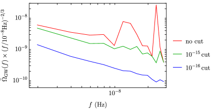
Figure 1: Background energy density $\bar{\Omega}_{\rm GW}(f)$ as function of frequency, for the three different cut-off values used in the filtering procedure.

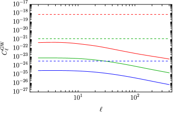
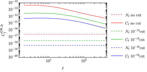
Figure 2: Angular power spectrum of auto-correlation (left panel) and cross-correlation (right panel) and corresponding shot noise contributions. The signal is integrated over the PTA frequency range.

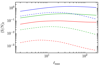
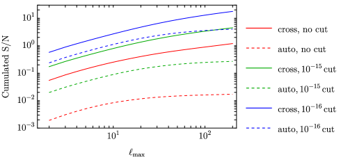
Figure 3: Left: SNR as function of the multipole $\ell$ of cross-correlation (dashed lines) and of auto-correlation (continuous lines) for an ideal experiment in which the shot noise is the only noise component. Right: corresponding cumulative SNR as function of $\ell_{\text{max}}$.

Fig. 2 represents for the three situations the angular power spectrum of auto- and cross-correlations, and the corresponding shot noise contributions. We see that while the auto-correlation map is shot noise dominated ($N^{\rm GW}_{\rm shot}\gg C_{\ell}^{\rm GW}$), the shot noise contribution to the cross-correlation is much suppressed ($N^{{\rm GW}\Delta}_{\rm shot}\ll C_{\ell}^{{\rm GW}\Delta}$). We observe that the filtering procedure reduces both the angular power spectrum of the clustering signal and the shot noise component, for both auto- and cross-angular power spectra.

In Fig. 3 (left panel) we show the SNR for auto- and cross-correlations (for the three cut-off values) as a function of the multipole $\ell$. On the right panel we show the corresponding cumulative SNR, as a function of $\ell_{\text{max}}$. As expected, the SNR of the cross-correlation outperforms the auto-correlation one (by more than two orders of magnitudes in the absence of a cut-off). This is due to the aforementioned hierarchy between signal and noise components along with $N^{\Delta}_{\rm shot}\ll C_{\ell}^{\Delta}$, i.e. the fact that the auto-correlation SNR scales as $\sqrt{2(2\ell+1)}C_{\ell}^{\text{GW}}/N_{\text{shot}}^{\text{GW}}$ whereas for cross-correlation it scales as $\sqrt{(2\ell+1)}C_{\ell}^{\text{GW}\Delta}/\sqrt{N_{\text{shot}}^{\text{GW}}C_{\ell}^{\Delta}}$.

We observe that even in the ideal case under study where the instrumental noise is set to zero (the noise is just shot noise), the SNR of single multipoles is never much larger than 1, unless a very low threshold of detection of single events is chosen. However, the cumulative SNR is above 1 already at $\ell_{\text{max}}=4$ (corresponding to $\sim 25$ pulsars), for a filtering threshold of $10^{-16}$, and it is above 1 for $\ell_{\text{max}}$=13 for a threshold of $10^{-15}$. This indicates that, while the reconstruction of the shape of the angular power spectrum will be challenging, it will be potentially possible to constrain the global amplitude of the spectrum, by combining the information from different multipoles.

We conclude observing that to obtain these results, we have fixed the value of the comoving galaxy number density equal to $a^{3}n_{\text{G}}=0.1$ Mpc^-3, however our results for the SNR depend very mildly on this choice. Indeed the SNR of the auto-correlation map does not depend on the galaxy number density assumed, while, for any reasonable value of $a^{3}n_{\text{G}}$, the dominant contribution to the noise of the cross-correlation map comes from the $\propto N_{\ell}^{\text{GW}}C_{\ell}^{\Delta}$ contribution in the denominator of eq. (29), which does not depend on the galaxy number density.

IV Discussion and conclusions

In this article, we explored the shot noise problem in the context of PTA observations, in isolation from other sources of noise. We derived from first principles the expression for the shot noise of the AGWB auto-correlation and the cross-correlation with a dense galaxy map. Using catalogs of massive BBH from Sesana (2013); Rosado et al. (2015), we showed that, unlike the auto-correlation, the cross-correlation map is not shot noise dominated: for an ideal experiment, the SNR of the cross-correlation outperforms the auto-correlation by more than two orders of magnitude. We also tested the effect of a filtering procedure that removes the brightest sources from the total background: this procedure further reduces shot noise, as the brightest sources dominate the background budget, obscuring the contribution of the unresolved population that traces the large-scale structure. A similar result was recently found in Semenzato et al. (2024), relying on numerical simulations. However, while our findings are consistent with the simulation results of Semenzato et al. (2024), our analytic treatment disagrees with the explanation proposed in that reference. In our derivations, we considered an ideal experiment with zero instrumental noise; however, when filtering out bright sources, we had to assume a threshold value to determine whether a source is resolvable individually. To do so, we considered the current EPTA sensitivity curve (effectively resulting in no resolvable sources), a threshold value corresponding to SKA sensitivity, and an intermediate scenario. We found that the amplitude of the angular power spectrum can potentially be detectable using cross-correlation with the galaxy distribution (integrated in redshift), when making use of a filtering procedure compatible with SKA projected sensitivity, and combining the first multipoles of the angular power spectrum up to $\ell_{\text{max}}=4$, requiring at least a number of pulsars $\sim 25$. With a sensitivity one order of magnitude lower than the projected SKA one, i.e. filtering out sources with $h_{\text{eff}}>10^{-15}$, the global amplitude of the anisotropies can be detected with $\ell_{\text{max}}$=13 requiring at least $\sim 200$ pulsars, which is more or less twice the number of pulsars currently monitored by the IPTA collaboration. Our results represent the best-case scenario for the detectability of the AGWB in the presence of spatial shot noise. A future study will be dedicated to deriving more realistic forecasts for future PTA experiments and galaxy surveys such as Euclid, properly factoring in the effects of instrumental noise and realistic filtering procedures.

Appendix A General properties of compound statistics

Let us consider $N$ being a random variable with variance $\langle N^{2}\rangle-\langle N\rangle^{2}$ and mean $\langle N\rangle$. Then for a generic function $f(N)$

$$\langle f(N)\rangle=\int f(N)p(N){\rm d}N\,.$$ (35)

We are interested in the statistics of the compound random variable $Y$ given by

$$Y=\sum_{i=1}^{N}X_{i}\,,$$ (36)

where $X_{i}$ is either $1$ or $0$, i.e. it is a binomial variable $X_{i}\sim B(1,\beta)$. It has a probability $p(Y)$, such that

$$p(Y)=\int p(Y|N)p(N){\rm d}N\,.$$ (37)

The conditional probability $p(Y|N)$ can be found from the fact that it is the sum of $N$ random variables (it is a convolution of probabilities), but we do not need to go to this level of sophistication to get convinced that

$$\langle Y\rangle_{N}=\int Yp(Y|N){\rm d}Y=N\langle X\rangle\,.$$ (38)

The subindex on the left hand side means that is an average at $N$ being fixed. For the second moment one has

$$\langle Y^{2}\rangle_{N}=\int Y^{2}p(Y|N){\rm d}Y=N\langle X^{2}\rangle+N(N-1)\langle X\rangle^{2}\,,$$ (39)

which is obtained by separation of the $X_{i}^{2}$ and the $X_{i}X_{j}$ with $i\neq j$.

We can work out the first moments of $Y$ from $p(Y)$. For a generic function of $Y$, we have

$$\langle f(Y)\rangle = \int f(Y)p(Y){\rm d}Y$$

$$= \int\int f(Y)p(Y|N)p(N){\rm d}N{\rm d}Y$$

$$= \int p(N){\rm d}N\left(\int f(Y)p(Y|N){\rm d}Y\right)$$

$$= \int\langle f(Y)\rangle_{N}\,p(N){\rm d}N\,,$$

where in the last line the remaining randomness of $N$ has to be treated. The average $\langle Y\rangle$ can be easily computed

$$\langle Y\rangle=\int\langle Y\rangle_{N}p(N){\rm d}N=\int\langle X\rangle Np(N){\rm d}N=\langle N\rangle\langle X\rangle\,.$$ (41)

Similarly for the second moment

$$\langle Y^{2}\rangle = \int\langle Y^{2}\rangle_{N}p(N){\rm d}N$$ (42)

$$= \int\left(N\langle X^{2}\rangle+N(N-1)\langle X\rangle^{2}\right)p(N){\rm d}N$$

$$= \langle N\rangle(\langle X^{2}\rangle-\langle X\rangle^{2})+\langle N^{2}\rangle\langle X\rangle^{2}\,.$$

Hence we obtain the variance of $Y$

$$\langle Y^{2}\rangle-\langle Y\rangle^{2} =\langle N\rangle(\langle X^{2}\rangle-\langle X\rangle^{2})+(\langle N^{2}\rangle-\langle N\rangle^{2})\langle X\rangle^{2}$$

$$=\langle N\rangle\langle X^{2}\rangle\,,\$$ (43)

where the last equality holds when $N$ is a Poisson variable. This derivation is valid whatever the statistics for $X$, and $\langle X^{2}\rangle=\langle X\rangle$ if $X\sim B(1,\beta)$. Following the same kind of reasoning we can also get cross correlations between $Y$ and $N$, and

$$\langle YN\rangle = \int\langle Y\rangle_{N}\,Np(N){\rm d}N$$ (44)

$$= \int\langle X\rangle N^{2}p(N){\rm d}N$$

$$= \langle X\rangle\langle N^{2}\rangle$$

$$= \langle X\rangle(\langle N\rangle+\langle N\rangle^{2})\,,$$

where the last equality holds when $N$ is Poisson variable. Then

$$\langle YN\rangle-\langle Y\rangle\langle N\rangle=\langle X\rangle\text{Var}(N)=\langle X\rangle\langle N\rangle\,,$$ (45)

where the last equality holds when $N$ is a Poisson variable.

Appendix B Signal to noise derivation

Let us assume that our observables are the angular power spectra of the AGWB and galaxy auto-correlations and their cross-correlation angular spectrum, i.e. $C_{\ell}^{\text{GW}}$, $C_{\ell}^{\Delta}$ and $C_{\ell}^{\text{GW}\Delta}$ are the observables. The estimator (full sky) of the angular power spectrum is

$$\hat{C}_{\ell}^{ab}=\frac{1}{2\ell+1}\sum_{m}a_{\ell m}^{a}(a_{\ell m}^{b})^{*}\,,$$ (46)

where $a_{\ell m}^{a,b}$ are Gaussian maps and the indices are defined as $a=(\text{GW},\Delta)$ and $b=(\text{GW},\Delta)$. We compute the covariance of this estimator. To make the notation compact, we introduce $X=(C_{\ell_{\text{min}}}^{\text{GW}},C_{\ell_{\text{min}}}^{\Delta},C_{\ell_{\text{min}}}^{\text{GW}\Delta},...,C_{\ell_{\text{max}}}^{\text{GW}},C_{\ell_{\text{max}}}^{\Delta},C_{\ell_{\text{max}}}^{\text{GW}\Delta})$. Then the associated covariance matrix is block diagonal

$$C=\left(\begin{array}[]{ccc}B_{\ell_{\text{min}}}&&0\\ &...&\\ 0&&B_{\ell_{\text{max}}}\\ \end{array}\right)\,,$$

with 3$\times$3 blocks

$$B_{\ell}=\frac{1}{2\ell+1}\times$$

$$\left(\begin{array}[]{ccc}2(C_{\ell}^{\text{GW}})^{2}&2(C_{\ell}^{\text{GW}\Delta})^{2}&2(C_{\ell}^{\text{GW}})(C_{\ell}^{\text{GW}\Delta})\\ 2(C_{\ell}^{\text{GW}\Delta})^{2}&2(C_{\ell}^{\Delta})^{2}&2(C_{\ell}^{\Delta})(C_{\ell}^{\text{GW}\Delta})\\ 2(C_{\ell}^{\text{GW}})(C_{\ell}^{\text{GW}\Delta})&2(C_{\ell}^{\Delta})(C_{\ell}^{\text{GW}\Delta})&C_{\ell}^{\text{GW}}C_{\ell}^{\Delta}+(C_{\ell}^{\text{GW}\Delta})^{2}\end{array}\right)\,,$$ (50)

where it is understood that each entry includes a noise part, i.e. one has to replace $C_{\ell}^{ab}\rightarrow C_{\ell}^{ab}+N_{\text{shot}}^{ab}$. We have all the ingredients to compute the (non-Gaussian) likelihood of the angular power spectra $X$ and compute the corresponding Fisher matrix deriving it with respect to the parameters $\theta_{a}$. The Fisher matrix is defined as

$$F_{ab}=\Big{<}-\frac{\partial^{2}\ln\mathcal{L}}{\partial\theta_{a}\partial\theta_{b}}\Big{>}\,,$$ (51)

where $\theta_{a}$ are a set of parameters of the model. It is possible to show that only the Gaussian part of the likelihood enters the Fisher matrix. We want to estimate the signal to noise of the galaxy map, hence we parametrize

$$X_{\ell}=(\mathcal{C}^{2}C_{\ell}^{\text{GW}}+N_{\text{shot}}^{\text{GW}},C_{\ell}^{\Delta}+N_{\text{shot}}^{\Delta},\mathcal{C}C_{\ell}^{\text{GW}\Delta}+N_{\text{shot}}^{\text{GW}\Delta})\,,$$ (52)

where $\mathcal{C}$ is a book keeping parameter for the amplitude. Then

$$\left(F_{\mathcal{C}}\right)_{\ell}=\left(\frac{S}{N}\right)_{\ell}^{2}=(\partial_{\mathcal{C}}X_{\ell})\cdot B_{\ell}^{-1}\cdot(\partial_{\mathcal{C}}X_{\ell})\,,$$ (53)

evaluated in ${\mathcal{C}}=1$. If we use only the information from the auto-correlation, we get (29) while using only cross-correlation we obtain (30).

Appendix C The GW energy density

Let us introduce some basic quantities that we extract from the catalog. The chirp mass of a source $\mathcal{M}$ is given by

$$\mathcal{M}=\frac{(m_{1}m_{2})^{3/5}}{(m_{1}+m_{2})^{1/5}}\,,$$ (54)

with $m_{1,2}$ the masses of the two black holes in the binary. We focus on the case of an inspiraling BBH, for which the emitted power is given by Maggiore (2007)

$$\frac{{\rm d}E_{s}}{{\rm d}t_{s}}=\frac{32}{5Gc^{5}}(\pi G\mathcal{M}f_{s})^{10/3}=\frac{32}{5Gc^{5}}(\pi G\mathcal{M}(1+z)f)^{10/3}\,,$$ (55)

where $E_{s}$ is the source-frame energy of one source with mass $\mathcal{M}$ and (source-frame) frequency $f_{s}$, and $t_{s}$ is the local cosmic time at the source. The source-frame frequency $f_{s}$ is related to the observed frequency by $f=f_{s}/(1+z)$. The observed power is found using $E_{o}=E_{s}/(1+z)$ and ${\rm d}t_{o}={\rm d}t_{s}(1+z)$, hence

$$\frac{{\rm d}E_{o}}{{\rm d}t_{o}}=\frac{1}{(1+z)^{2}}\frac{{\rm d}E_{s}}{{\rm d}t_{s}}\,.$$ (56)

We denote the (comoving) number of sources per comoving volume ${\rm d}V_{c}$, per frequency ${\rm d}f$ and per logarithmic chirp mass ${\rm d}\log{\mathcal{M}}$ by

$$a^{3}n_{s}(\mathbf{n},z,\mathcal{M},f)\equiv f\frac{{\rm d}N_{s}}{{\rm d}V_{c}\,{\rm d}\log(\mathcal{M})\,{\rm d}f}\propto f^{-8/3}\,,$$ (57)

where $N_{s}$ is the number of sources. The previous scaling in frequency is found using that the number of sources in a given frequency band is proportional to the time spent in that band, along with ${\rm d}\log f/{\rm d}t\propto f^{8/3}$. We split this quantity into an angle-averaged term $\bar{n}_{s}$ and an anisotropic contribution

$$n_{s}(\mathbf{n},z,\mathcal{M},f)=\bar{n}_{s}(z,\mathcal{M},f)+\delta n_{s}(\mathbf{n},z,\mathcal{M},f)\,.$$ (58)

To consider the contributions of the different directions $\mathbf{n}$ to the total energy density parameter at the observer, we then analogously split $\Omega_{\rm GW}$ in an angle-averaged term $\bar{\Omega}_{\rm GW}$ and an anisotropic fluctuation, with the definition (1). The isotropic part is obtained by summing all contributions as in (2a) with

$$\partial_{r}\bar{\Omega}_{\text{GW}}(f,r)=\frac{f{\cal A}(f,r)}{\rho_{c}}=\int{\rm d}\log\mathcal{M}\frac{\partial\bar{\Omega}_{\rm GW}(f,r,\mathcal{M})}{\partial r\partial\log\mathcal{M}}\,,$$ (59)

where

$$\frac{\partial\bar{\Omega}_{\rm GW}(f,r,\mathcal{M})}{\partial r\partial\log\mathcal{M}}=\frac{1}{\rho_{c}}\frac{1}{(1+z)^{2}}\frac{{\rm d}E_{s}}{{\rm d}t_{s}}a^{3}\bar{n}_{s}(z,\mathcal{M},f)\,,$$ (60)

and the function $z=z(r)$ must be used to relate a given redshift $z$ to the conformal distance $r$.

Denoting the fractional fluctuation in the number density of sources by

$$\delta_{s}(\mathbf{n},z,\mathcal{M})=\frac{\delta n_{s}(\mathbf{n},z,\mathcal{M},f)}{\bar{n}_{s}(z,\mathcal{M},f)}\,,$$ (61)

and using that the GW sources are biased tracers of the underlying distribution of galaxies,

$$\delta_{s}(\mathbf{n},z,\mathcal{M})=b_{s}(z,\mathcal{M})\delta_{g}(\mathbf{n},z)\,,$$ (62)

we obtain

$$\delta\Omega_{\rm GW}(f,\mathbf{n}) =\frac{1}{4\pi}\int{\rm d}r\int{\rm d}\log\mathcal{M}$$

$$\times\frac{\partial\bar{\Omega}_{\rm GW}(f,r,\mathcal{M})}{\partial r\partial\log\mathcal{M}}b_{s}(z,\mathcal{M})\,\delta_{g}(\mathbf{n},z)\,,$$ (63)

where the integration on the conformal distance $r$ can be replaced by an integral on redshifts using the background cosmology and ${\rm d}r={\rm d}z/H(z)$.

Eq. (63) relates the anisotropies in the energy density of an astrophysical SGWB to the anisotropies of the large-scale structure where SGWB sources are found. We assume that GW sources follow the same clustering structure as the galaxies, hence we take $b_{s}=1$ in our analysis.

Appendix D Energy density and shot noise from a catalogue

For a given source $i$, we introduce the following quantity $P_{i}\equiv({\rm d}E_{o}/{\rm d}t_{o})_{i}/\rho_{c}=({\rm d}E_{s}/{\rm d}t_{s})_{i}/\rho_{c}/(1+z_{i})^{2}$, such that for a collection of $N$ sources in directions $\mathbf{n}_{i}$

$$\Omega_{\rm GW}(\mathbf{n})=\sum_{i=1}^{N}\left(\frac{P_{i}}{4\pi r_{i}^{2}}\right)\delta^{2}(\mathbf{n},\mathbf{n}_{i})\,.$$ (64)

Using

$$\delta^{2}(\mathbf{n}_{1},\mathbf{n}_{2})=\sum_{\ell m}Y_{\ell m}(\mathbf{n}_{1})Y^{\star}_{\ell m}(\mathbf{n}_{2})\,,$$ (65)

and an expansion $\Omega_{\rm GW}(\mathbf{n})=\sum_{\ell m}\Omega_{\ell m}^{\rm GW}Y_{\ell m}(\mathbf{n})$ we get

$$\Omega^{\rm GW}_{\ell m}=\sum_{i=1}^{N}\left(\frac{P_{i}}{4\pi r_{i}^{2}}\right)Y^{\star}_{\ell m}(\mathbf{n}_{i})\,.$$ (66)

An estimator of the $C^{\rm GW}_{\ell}$ defined in (5a) is

$$\hat{C}^{\rm GW}_{\ell}=\frac{1}{2\ell+1}\sum_{m=-\ell}^{\ell}\Omega^{\rm GW}_{\ell m}\Omega^{{\rm GW}\star}_{\ell m}\,,$$ (67)

and for random positions of the sources, that is sources which are not located according to clustering properties, it is non-vanishing only due to the Poissonian nature of the source distribution. We want to average this estimator over the direction realizations of the sources, that is over random realizations of the set of directions $\{\mathbf{n}_{i}\}$, so as to estimate the shot noise. We shall use that (see e.g. Allen et al. (2024) or appendix D of Pitrou and Cusin (2024))

$$\langle Y_{\ell m}(\mathbf{n}_{i_{1}})\rangle_{\{\mathbf{n}_{i}\}}=\frac{\delta_{\ell}^{0}\delta_{m}^{0}}{\sqrt{4\pi}}\,,$$ (68)

and for $(\ell,m)\neq(0,0)$

$$\langle Y_{\ell m}(\mathbf{n}_{i_{1}})Y^{\star}_{\ell^{\prime}m^{\prime}}(\mathbf{n}_{i_{1}})\rangle_{\{\mathbf{n}_{i}\}}=\frac{\delta_{\ell\ell^{\prime}}\delta_{mm^{\prime}}}{4\pi}\,.$$ (69)

Then when averaging over all random positions of these $N$ sources

$$4\pi\langle\Omega_{\rm GW}(\mathbf{n})\rangle_{\{\mathbf{n}_{i}\}} =\sqrt{4\pi}\langle\Omega^{\rm GW}_{00}\rangle_{\{\mathbf{n}_{i}\}}=\sum_{i=1}^{N}\frac{P_{i}}{4\pi r_{i}^{2}}\,,$$ (70)

$$\langle\hat{C}^{\rm GW}_{\ell}\rangle_{\{\mathbf{n}_{i}\}} =\frac{1}{4\pi}\sum_{i=1}^{N}\left(\frac{P_{i}}{4\pi r_{i}^{2}}\right)^{2}\,.$$ (71)

We identify the average GW density as $\bar{\Omega}_{\rm GW}=4\pi\langle\Omega_{\rm GW}(\mathbf{n})\rangle_{\{\mathbf{n}_{i}\}}$ and shot noise with $N_{\rm shot}^{\rm GW}=\langle\hat{C}^{\rm GW}_{\ell}\rangle_{\{\mathbf{n}_{i}\}}$.

In order to check the consistency with the continuous integral formulas we use

$$\sum_{i=1}^{N}\to\int{\rm d}\log f\int{\rm d}\log\mathcal{M}\int{\rm d}r(4\pi r^{2}a^{3}\bar{n}_{s})\,,$$ (72)

and indeed applying this replacement rule to (70) we get (60). Also for shot noise we get

$$\langle\hat{C}^{\rm GW}_{\ell}\rangle_{\{\mathbf{n}_{i}\}} \simeq\int{\rm d}\log f\int{\rm d}\log\mathcal{M}\int{\rm d}ra^{3}\bar{n}_{s}r^{2}\left(\frac{P}{4\pi r^{2}}\right)^{2}$$ (73)

$$\simeq\int{\rm d}\log f\int{\rm d}\log\mathcal{M}\int{\rm d}r\frac{a^{3}\bar{n}_{s}}{(4\pi)^{2}r^{2}}\left(\frac{{\rm d}E_{s}/{\rm d}t_{s}}{(1+z)^{2}\rho_{c}}\right)^{2}\,,$$

and using (60) we recover (26). Hence when using a catalog, we have to use (70) to estimate the background GW density, and (71) to estimate the shot noise.

References

- Agazie et al. (2023a) G. Agazie et al. (NANOGrav), Astrophys. J. Lett. 951, L8 (2023a), arXiv:2306.16213 [astro-ph.HE] .
- Reardon et al. (2023) D. J. Reardon et al., Astrophys. J. Lett. 951, L6 (2023), arXiv:2306.16215 [astro-ph.HE] .
- Antoniadis et al. (2023) J. Antoniadis, P. Arumugam, S. Arumugam, S. Babak, M. Bagchi, A.-S. Bak Nielsen, C. G. Bassa, A. Bathula, A. Berthereau, M. Bonetti, E. Bortolas, P. R. Brook, M. Burgay, R. N. Caballero, A. Chalumeau, D. J. Champion, S. Chanlaridis, S. Chen, I. Cognard, S. Dandapat, D. Deb, S. Desai, G. Desvignes, N. Dhanda-Batra, C. Dwivedi, M. Falxa, R. D. Ferdman, A. Franchini, J. R. Gair, B. Goncharov, A. Gopakumar, E. Graikou, J.-M. Grießmeier, L. Guillemot, Y. J. Guo, Y. Gupta, S. Hisano, H. Hu, F. Iraci, D. Izquierdo-Villalba, J. Jang, J. Jawor, G. H. Janssen, A. Jessner, B. C. Joshi, F. Kareem, R. Karuppusamy, E. F. Keane, M. J. Keith, D. Kharbanda, T. Kikunaga, N. Kolhe, M. Kramer, M. A. Krishnakumar, K. Lackeos, K. J. Lee, K. Liu, Y. Liu, A. G. Lyne, J. W. McKee, Y. Maan, R. A. Main, M. B. Mickaliger, I. C. Niţu, K. Nobleson, A. K. Paladi, A. Parthasarathy, B. B. P. Perera, D. Perrodin, A. Petiteau, N. K. Porayko, A. Possenti, T. Prabu, H. Quelquejay Leclere, P. Rana, A. Samajdar, S. A. Sanidas, A. Sesana, G. Shaifullah, J. Singha, L. Speri, R. Spiewak, A. Srivastava, B. W. Stappers, M. Surnis, S. C. Susarla, A. Susobhanan, K. Takahashi, P. Tarafdar, G. Theureau, C. Tiburzi, E. van der Wateren, A. Vecchio, V. Venkatraman Krishnan, J. P. W. Verbiest, J. Wang, L. Wang, and Z. Wu, , A50 (2023).
- Xu et al. (2023) H. Xu et al., Res. Astron. Astrophys. 23, 075024 (2023), arXiv:2306.16216 [astro-ph.HE] .
- Romano and Cornish (2016) J. D. Romano and N. J. Cornish, (2016), arXiv:1608.06889 [gr-qc] .
- Jenet and Romano (2015) F. A. Jenet and J. D. Romano, Am. J. Phys. 83, 635 (2015), arXiv:1412.1142 [gr-qc] .
- Romano and Allen (2023) J. D. Romano and B. Allen, (2023), arXiv:2308.05847 [gr-qc] .
- Grimm et al. (2024a) N. Grimm, M. Pijnenburg, G. Cusin, and C. Bonvin, (2024a), arXiv:2411.08744 [gr-qc] .
- Grimm et al. (2024b) N. Grimm, M. Pijnenburg, G. Cusin, and C. Bonvin, (2024b), arXiv:2404.05670 [astro-ph.CO] .
- Anholm et al. (2009) M. Anholm, S. Ballmer, J. D. E. Creighton, L. R. Price, and X. Siemens, Phys. Rev. D 79, 084030 (2009), arXiv:0809.0701 [gr-qc] .
- Mingarelli et al. (2013) C. M. F. Mingarelli, T. Sidery, I. Mandel, and A. Vecchio, Phys. Rev. D 88, 062005 (2013), arXiv:1306.5394 [astro-ph.HE] .
- Depta et al. (2024) P. F. Depta, V. Domcke, G. Franciolini, and M. Pieroni, (2024), arXiv:2407.14460 [astro-ph.CO] .
- Semenzato et al. (2024) F. Semenzato, J. A. Casey-Clyde, C. M. F. Mingarelli, A. Raccanelli, N. Bellomo, N. Bartolo, and D. Bertacca, (2024), arXiv:2411.00532 [astro-ph.CO] .
- Bernardo et al. (2024) R. C. Bernardo, G.-C. Liu, and K.-W. Ng, JCAP 04, 034 (2024), arXiv:2312.03383 [gr-qc] .
- Cusin et al. (2019a) G. Cusin, R. Durrer, and P. G. Ferreira, Phys. Rev. D 99, 023534 (2019a), arXiv:1807.10620 [astro-ph.CO] .
- Grunthal et al. (2024) K. Grunthal et al., (2024), 10.1093/mnras/stae2573, arXiv:2412.01214 [astro-ph.HE] .
- Agazie et al. (2024a) G. Agazie et al., (2024a), arXiv:2411.13472 [astro-ph.HE] .
- Gair et al. (2014) J. Gair, J. D. Romano, S. Taylor, and C. M. F. Mingarelli, Phys. Rev. D 90, 082001 (2014), arXiv:1406.4664 [gr-qc] .
- Roebber and Holder (2017) E. Roebber and G. Holder, Astrophys. J. 835, 21 (2017), arXiv:1609.06758 [astro-ph.CO] .
- Qin et al. (2019) W. Qin, K. K. Boddy, M. Kamionkowski, and L. Dai, Phys. Rev. D 99, 063002 (2019), arXiv:1810.02369 [astro-ph.CO] .
- Hotinli et al. (2019) S. C. Hotinli, M. Kamionkowski, and A. H. Jaffe, Open J. Astrophys. 2, 8 (2019), arXiv:1904.05348 [astro-ph.CO] .
- Nay et al. (2024) J. Nay, K. K. Boddy, T. L. Smith, and C. M. F. Mingarelli, Phys. Rev. D 110, 044062 (2024), arXiv:2306.06168 [gr-qc] .
- Bernardo and Ng (2022) R. C. Bernardo and K.-W. Ng, JCAP 11, 046 (2022), arXiv:2209.14834 [gr-qc] .
- Bernardo and Ng (2023) R. C. Bernardo and K.-W. Ng, Phys. Rev. D 107, 044007 (2023), arXiv:2208.12538 [gr-qc] .
- Allen (2024) B. Allen, (2024), arXiv:2404.05677 [gr-qc] .
- Bernardo and Ng (2024) R. C. Bernardo and K.-W. Ng, (2024), arXiv:2409.07955 [astro-ph.CO] .
- Pitrou and Cusin (2024) C. Pitrou and G. Cusin, (2024), arXiv:2412.12073 [gr-qc] .
- Siemens et al. (2013) X. Siemens, J. Ellis, F. Jenet, and J. D. Romano, Class. Quant. Grav. 30, 224015 (2013), arXiv:1305.3196 [astro-ph.IM] .
- Pol et al. (2022) N. Pol, S. R. Taylor, and J. D. Romano, Astrophys. J. 940, 173 (2022), arXiv:2206.09936 [astro-ph.HE] .
- Agazie et al. (2023b) G. Agazie et al. (NANOGrav), Astrophys. J. Lett. 956, L3 (2023b), arXiv:2306.16221 [astro-ph.HE] .
- Rajagopal and Romani (1995) M. Rajagopal and R. W. Romani, Astrophys. J. 446, 543 (1995), arXiv:astro-ph/9412038 [astro-ph] .
- Jaffe and Backer (2003) A. H. Jaffe and D. C. Backer, Astrophys. J. 583, 616 (2003), arXiv:astro-ph/0210148 [astro-ph] .
- Sesana et al. (2008) A. Sesana, A. Vecchio, and C. N. Colacino, MNRAS 390, 192 (2008), arXiv:0804.4476 .
- Falxa et al. (2025) M. Falxa, H. Q. Leclere, and A. Sesana, Phys. Rev. D 111, 023047 (2025), arXiv:2412.01899 [gr-qc] .
- Jenkins and Sakellariadou (2019) A. C. Jenkins and M. Sakellariadou, (2019), arXiv:1902.07719 [astro-ph.CO] .
- Jenkins et al. (2019) A. C. Jenkins, J. D. Romano, and M. Sakellariadou, Phys. Rev. D 100, 083501 (2019).
- Alonso et al. (2020) D. Alonso, G. Cusin, P. G. Ferreira, and C. Pitrou, Phys. Rev. D 102, 023002 (2020), arXiv:2002.02888 [astro-ph.CO] .
- Cusin et al. (2019b) G. Cusin, I. Dvorkin, C. Pitrou, and J.-P. Uzan, Phys. Rev. D 100, 063004 (2019b), arXiv:1904.07797 [astro-ph.CO] .
- Yang et al. (2023) K. Z. Yang, J. Suresh, G. Cusin, S. Banagiri, N. Feist, V. Mandic, C. Scarlata, and I. Michaloliakos, Phys. Rev. D 108, 043025 (2023), arXiv:2304.07621 [gr-qc] .
- Alonso et al. (2024) D. Alonso, M. Nikjoo, A. I. Renzini, E. Bellini, and P. G. Ferreira, Phys. Rev. D 110, 103544 (2024), arXiv:2406.19488 [astro-ph.CO] .
- Cusin et al. (2018) G. Cusin, C. Pitrou, and J.-P. Uzan, Phys. Rev. D97, 123527 (2018), arXiv:1711.11345 [astro-ph.CO] .
- Cusin et al. (2017) G. Cusin, C. Pitrou, and J.-P. Uzan, Phys. Rev. D96, 103019 (2017), arXiv:1704.06184 [astro-ph.CO] .
- Pitrou et al. (2020) C. Pitrou, G. Cusin, and J.-P. Uzan, Phys. Rev. D 101, 081301 (2020), arXiv:1910.04645 [astro-ph.CO] .
- Sesana (2013) A. Sesana, MNRAS 433, L1 (2013), arXiv:1211.5375 [astro-ph.CO] .
- Rosado et al. (2015) P. A. Rosado, A. Sesana, and J. Gair, Mon. Not. Roy. Astron. Soc. 451, 2417 (2015), arXiv:1503.04803 [astro-ph.HE] .
- Rosado and Sesana (2014) P. A. Rosado and A. Sesana, MNRAS 439, 3986 (2014), arXiv:1311.0883 [astro-ph.CO] .
- Muzzin et al. (2013) A. Muzzin, D. Marchesini, M. Stefanon, M. Franx, H. J. McCracken, B. Milvang-Jensen, J. S. Dunlop, J. P. U. Fynbo, G. Brammer, I. Labbé, and P. G. van Dokkum, Astrophys. J. 777, 18 (2013), arXiv:1303.4409 [astro-ph.CO] .
- de Ravel et al. (2009) L. de Ravel, O. Le Fèvre, L. Tresse, D. Bottini, B. Garilli, V. Le Brun, D. Maccagni, R. Scaramella, M. Scodeggio, G. Vettolani, A. Zanichelli, C. Adami, S. Arnouts, S. Bardelli, M. Bolzonella, A. Cappi, S. Charlot, P. Ciliegi, T. Contini, S. Foucaud, P. Franzetti, I. Gavignaud, L. Guzzo, O. Ilbert, A. Iovino, F. Lamareille, H. J. McCracken, B. Marano, C. Marinoni, A. Mazure, B. Meneux, R. Merighi, S. Paltani, R. Pellò, A. Pollo, L. Pozzetti, M. Radovich, D. Vergani, G. Zamorani, E. Zucca, M. Bondi, A. Bongiorno, J. Brinchmann, O. Cucciati, S. de La Torre, L. Gregorini, P. Memeo, E. Perez-Montero, Y. Mellier, P. Merluzzi, and S. Temporin, Astronomy and Astrophysics 498, 379 (2009), arXiv:0807.2578 [astro-ph] .
- Kitzbichler and White (2008) M. G. Kitzbichler and S. D. M. White, MNRAS 391, 1489 (2008), arXiv:0804.1965 [astro-ph] .
- Kormendy and Ho (2013) J. Kormendy and L. C. Ho, Annual Review of Astronomy and Astrophysics 51, 511 (2013), arXiv:1304.7762 [astro-ph.CO] .
- Sesana et al. (2008) A. Sesana, A. Vecchio, and C. N. Colacino, Mon. Not. Roy. Astron. Soc. 390, 192 (2008), arXiv:0804.4476 [astro-ph] .
- Marin et al. (2013) F. A. Marin et al. (WiggleZ), Mon. Not. Roy. Astron. Soc. 432, 2654 (2013), arXiv:1303.6644 [astro-ph.CO] .
- Rassat et al. (2008) A. Rassat, A. Amara, L. Amendola, F. J. Castander, T. Kitching, M. Kunz, A. Refregier, Y. Wang, and J. Weller, (2008), arXiv:0810.0003 [astro-ph] .
- Agazie et al. (2024b) G. Agazie et al. (International Pulsar Timing Array), Astrophys. J. 966, 105 (2024b), arXiv:2309.00693 [astro-ph.HE] .
- Truant et al. (2024) R. J. Truant, D. Izquierdo-Villalba, A. Sesana, G. Mohiuddin Shaifullah, and M. Bonetti, arXiv e-prints , arXiv:2407.12078 (2024), arXiv:2407.12078 [astro-ph.GA] .
- Sah and Mukherjee (2024) M. R. Sah and S. Mukherjee, (2024), arXiv:2407.11669 [astro-ph.CO] .
- Maggiore (2007) M. Maggiore, Gravitational Waves. Vol. 1: Theory and Experiments, Oxford Master Series in Physics (Oxford University Press, 2007).
- Allen et al. (2024) B. Allen, D. Agarwal, J. D. Romano, and S. Valtolina, Phys. Rev. D 110, 123507 (2024), arXiv:2406.16031 [gr-qc] .