Accounting for the Known Unkown: A Parametric Framework to Incorporate Systematic Waveform Errors in Gravitational-Wave Parameter Estimation

Abstract

The parameter estimation (PE) for gravitational wave (GW) merger events relies on a waveform model calibrated using numerical simulations. Within the Bayesian framework, this waveform model represents the GW signal produced during the merger and is crucial for estimating the likelihood function. However, these waveform models may possess systematic errors that can differ across the parameter space. Addressing these errors in the current data analysis pipeline is an active area of research. This work presents a framework for accounting for uncertainties in waveform modeling. We introduce two parametrizations, relative and absolute errors in the phase of the waveform, to modify the base waveform model, which can account for uncertainties. When the waveform errors are known, those error budgets can be used as a prior distribution in the Bayesian framework. We also show that conservative priors can be used to quantify uncertainties in waveform modeling without any knowledge of waveform error budgets. By conducting zero-noise injections and recoveries, we demonstrate through PE results that even 1-2% of errors in relative phase to the actual waveform model can introduce biases in the recovered parameters. These biases can be corrected when we account for waveform uncertainties within the PE framework. By injecting a series of precessing waveform models and using the nonspinning model for recovery, we show that our method can account for the missing physics by making the posterior samples broad enough to account for bias. We also present a Python package that is easily integrated with the publicly available GW analysis tool PyCBC and can be used to do PE with the parametrization presented in this paper.

I Introduction

GW signals from compact binary merger events provide us with a unique opportunity to probe these highly energetic events. With the network of advanced GW detectors, including the LIGO detectors in Hanford and Livingston, USA, the Virgo detector in Italy, and the KAGRA detector in Japan, the detection of GW signals has become routine (Aasi et al., 2015; Buikema et al., 2020; Abbott et al., 2016a; Acernese et al., 2015, 2019). Recent catalogs of GW mergers, compiled from the data analysis of the first three observation runs of the LIGO and Virgo detectors, compile over 90 merger events. These catalogs include the analysis from the LIGO-Virgo-KAGRA (LVK) collaboration (The LIGO Scientific Collaboration et al., 2021a), as well as analyses conducted by other independent groups (Nitz et al., 2023; Wadekar et al., 2023). The emphasis of the GW community has now expanded from detection to precision science, such as constraining the theory of general relativity (Abbott et al., 2021a), inferring the astrophysical distribution of the population of compact binary mergers (Abbott et al., 2023a; Nitz et al., 2023), inferring Hubble constant (Abbott et al., 2021b), constraining the equation of state of a neutron star (Abbott et al., 2018, 2019a; Capano et al., 2020), etc.

The detection of GWs and the precision of measurements of source properties relies on the accurate modeling of the signals from the merger of compact binary systems such as binary black holes (BBH), binary neutron stars (BNS), and neutron star-black hole (NSBH). These waveform models have been developed over the years with the help of Post-Newtonian (PN) analytical calculation for the early inspiral part of the signals (Blanchet, 2014), and they rely on calibration from Numerical relativity (NR) simulations for merger and ringdown regimes (Campanelli et al., 2006; Pretorius, 2005; Baker et al., 2006). The signal’s loudness and detector sensitivity determine the width of statistical uncertainties in the measurement, while the inaccuracies in the waveform models could lead to systematic errors. The statistical uncertainties go down as the detectors become more and more sensitive while systematic errors remain the same.

In the coming years, the planned upgrades to existing detectors (Abbott et al., 2016a, b) and the addition of new ones, such as LIGO India (Saleem et al., 2022), are expected to enhance the sensitivity of the detector network. Efforts are currently underway to develop third-generation (3G) detectors, such as the Einstein Telescope (ET) (Punturo et al., 2010; Hild et al., 2011) and Cosmic Explorer (CE) (Evans et al., 2021; Srivastava et al., 2022; Evans et al., 2023), over the next decade. These 3G detectors are anticipated to be significantly more sensitive—by an order of magnitude—than the current generation of detectors, and they are expected to enhance low-frequency sensitivity. As the GW detectors’ sensitivities keep improving, the waveform modeling community tries to keep up with the required accuracy to provide unbiased estimates.

One important question is how accurate waveform models need to be. One may not want to burden the waveform modeling and NR simulation community with generating waveform models much better than the analysis can resolve (Lindblom et al., 2008). However, studies suggest that we are already reaching the point where we can not ignore the systematic bias in a fraction of loud events. In a recent study, (Pürrer and Haster, 2020) it is shown that the typical biases in the inferred source parameters will be roughly equivalent to the standard deviation for the design sensitivity of current-generation detectors, and these biases could increase significantly for third-generation (3G) detectors. While a small bias in the fraction of events may be irrelevant for some studies, it could be critical for those that depend on accurate estimates of source properties. This is particularly true for inferring population characteristics of BBH mergers Dhani et al. (2024a), estimating the Hubble constant using localization volume, issuing pre-merger localization alerts Kumar et al. (2022), and conducting tests of general relativity (Gupta et al., 2024), among others.

The impacts of the waveform modeling accuracy on estimating the source parameters have been extensively studied (Lindblom et al., 2008; Pürrer and Haster, 2020; Read, 2023; Dhani et al., 2024a). The standard approach to account for waveform systematics is combining the posterior samples from different waveform models by assigning appropriate weights (Abbott et al., 2023b; Ashton and Khan, 2020; Jan et al., 2020) or using hyperparameters to sample over different waveform approximants at the likelihood evaluation level (Ashton and Dietrich, 2022; Hoy, 2022; Puecher et al., 2024; Samajdar and Dietrich, 2018, 2019; Hoy et al., 2024). These approaches are expected to marginalize potential differences between different waveform approximants. However, if all the waveform models have similar systematic effects, their difference would not accurately represent the true systematics in each model. Another approach is to marginalize the uncertainties using prior distributions analytically. These priors can be constructed using the Gaussian processes regression technique from a training set of accurate templates (Moore and Gair, 2014). Similar techniques can also be applied to address the waveform systematics arising from calibration with NR simulations (Pompili et al., 2024; Bachhar et al., 2024). There are also approaches to provide probabilistic models for the waveform, which can be used in sampling with appropriate weights (Khan, 2024). The authors in (Owen et al., 2023) marginalize over higher order PN terms to mitigate the systematic errors.

This work presents a general framework that accounts for the uncertainties in waveform modeling through parametric models. The additional parameters in PE analysis relate to the waveform’s amplitude and phase errors. When we know the expected amplitude and phase error distribution in the waveform as a function of frequency, we can use them as priors in PE analysis. These errors are expected to be a function of parameter space. In the absence of such knowledge, we can be agnostic and use wider priors to capture any possible deviation. We evaluate this framework by introducing arbitrary deviations into reference waveform models and recovering them through our data analysis pipeline. In addition to correcting for biases, we assess the method’s ability to quantify the nature of deviations from the true signal, particularly for the higher signal-to-noise ratio (SNR) ”golden” binary systems.

This paper is structured as follows: Section II reviews current techniques used in waveform model developments and the potential sources of systematic biases they might contain. Section III visits the state-of-the-art PE techniques and also discusses current methods to deal with waveform systematics. Section IV discusses modeling GW strain data from the detector and introduces the parametrizations that we use in this work to account for waveform errors in PE. The following section (section V) discusses the Fisher matrix approach to account for the systematic bias. We also discuss the limitations where the Fisher matrix approach is no longer valid, and we need to do a full PE analysis. In section VI, we present the detailed simulations followed by an injection-recovery campaign to test the validity of this method. We also discuss the scenario where we can use these parametric models to account for the missing physical effects not considered in the waveform model. In the end, we discuss the findings of the work and summarize them in section VII. If the reader is already familiar with the PE techniques and the potential sources of errors, they may skip Section III. Additionally, if the reader is acquainted with the Fisher matrix approach for correcting systematic biases and understands its limitations in specific scenarios, they can skip Section V. The reader who is just interested in the methodology and results can read sections IV, VI, and VII in that order.

II Waveform Modelling and Sources of Uncertainties

The GW signal of compact binary mergers can be predicted by solving Einstein’s Equations for the two-body problem in the general theory of relativity. However, due to the complexity of these equations, some form of approximations need to be employed to model binary systems. The most sophisticated models combine several modeling techniques. A review of those techniques and models is beyond the scope of this paper, but we give a brief overview of aspects that are relevant to our discussion of systematic waveform errors. Here we focus on black-hole binaries on quasi-circular orbits, as they are the most frequent source of detected GWs. However, many considerations detailed below apply to more general binary sources as well.

A black hole binary and its emitted GW signal are described by several parameters, such as the BH component masses ($m_{1},m_{2}$), their spins ($\vec{s}_{1},\vec{s}_{2}$), luminosity distance ($D_{L}$), inclination of binary plane with the line of sight ($\iota$), polarization angle with respect to the detector ($\psi$), coalescence phase of the binary ($\phi$), right ascension (RA) and declination angle (dec) in the sky, and the coalescence time ($t_{c}$).

When the binary constituents are widely separated and their velocities are small (compared to the speed of light), the system’s evolution can be approximately modeled by a power series expansion. The most commonly used approach is the PN formalism that expands in the system’s relative velocity (see Blanchet (2014) for a review). Alternative approaches exist, for example the post-Minkowskian formalism expands in the gravitational constant G Detweiler and Brown (1997); Bern et al. (2019). In the highly relativistic regime, where the spacetime curvature is large and velocities are high, these approaches become inaccurate. More concretely, PN expansions are well suited to describe the early inspiral of a black-hole binary, but as the black holes approach each other and their velocities increase, purely PN models become inaccurate and unable to describe the merger and post-merger stages.

While the post-merger ringdown of the remnant black hole can be well described by perturbation theory Vishveshwara (1970); Chandrasekhar and Detweiler (1975), the merger itself can only be modeled by numerically solving Einstein’s Equation. Since its breakthrough Pretorius (2005); Campanelli et al. (2006); Baker et al. (2006), NR has become an important, well established tool in GW astronomy. However, because of its computational complexity, NR simulation can only cover the late inspiral (typically a few tens of orbits), merger and ringdown of the binary coalescence.

Neither of the above mentioned approaches can model the entire GW signal of interest. PN models become inaccurate towards the merger and do not include any merger or ringdown portion. NR is computationally too expensive and cannot cover hundreds or even thousands of orbits before merger. Therefore, several model approaches have been designed to bridge the gap between numerical and analytical methods Ohme (2012).

Three model families are regularly employed in the analysis of GW observations Abbott et al. (2023b). The phenomenological models Ajith et al. (2008, 2011); Santamaria et al. (2010); Khan et al. (2016, 2019, 2020); Husa et al. (2016); London et al. (2018); Hannam et al. (2014); García-Quirós et al. (2020); Pratten et al. (2021, 2020); Estellés et al. (2021, 2022); Ghosh et al. (2024); Thompson et al. (2024) are based on a set of hybrid waveforms that smoothly connect analytically derived inspiral signals with NR data. This data set is then described by PN inspired phenomenological formulae with tune-able coefficients that fit across the binary’s parameter space. The resulting model is a set of closed-form expressions that describe the amplitude and phase of the GW signal.

Another approach is based on the effective-one-body (EOB) formalism Buonanno and Damour (1999), in which the binary system is mapped to a Hamiltonian formulation of a particle orbiting in an effective potential. By introducing higher-order terms and tune-able coefficients that are fit to waveforms from NR simulations, the resulting EOBNR waveforms can describe the binary coalescence accurately up to the merger. Completed by a suitable ringdown attachment, several models of the EOBNR family have been developed Pan et al. (2011, 2014); Taracchini et al. (2014); Bohé et al. (2017); Cotesta et al. (2018); Ossokine et al. (2020); Pompili et al. (2023); Gamboa et al. (2024); Damour et al. (2013); Gamba et al. (2021); Nagar et al. (2024) and applied to the analysis of GW events.

The third model family is called surrogate models. These models are built by decomposing waveform data from NR simulations into a suitable basis and interpolating between them Field et al. (2014). NR surrogate models Blackman et al. (2017a, b); Varma et al. (2019a, b) are very faithful to the NR simulations they were built from, but they are limited by the length and parameter coverage of NR simulations.

All of the modeling approaches approximate the exact solutions of Einstein’s Equation. Therefore, they carry systematic uncertainties that are difficult to quantify in their entirety. Numerical simulations start with approximate initial data and discretize the spacetime. The resulting resolution error is often estimated by providing simulation results of the same system for different resolutions. All modeling approaches described above rely on input from numerical simulations, but they also need to interpolate between different simulations to cover the entire parameter space of interest. This interpolation introduces additional inaccuracies that are often less well quantified. Part of the problem is not only the interpolation (or even extrapolation) of existing NR data. The ansatz used to describe the data carries its own limitations, whether it is data driven (such as Gaussian process regression) or analytically motivated.

In summary, all modeling approaches have to balance representing known NR simulation data as accurately as possible while ensuring a smooth and robust interpolation across the parameter space. The techniques employed to accomplish this have advanced over the years, but they cannot be perfect. Therefore, any model’s prediction has to be treated as a “best-guess” waveform for each set of parameters. While the faithfulness to NR data is often very impressive, one must not forget the uncertainties arising from each step of the modeling process.

Here we discuss and test a framework that moves away from the “best-guess” paradigm to accounting for uncertain signal predictions in parameter-estimation analyses.

III Parameter Estimation

In this section, we review the PE techniques for GW data analysis and potential errors in estimating source properties. Readers who are familiar with this can skip to the next section. Time series strain data $s(t)$ in each detector consists of noise $n(t)$ and may contain a transient signal $h(t)$. It is assumed that when the signal is present, the noise and signal are additive to give the strain data, i.e.

$$s(t)=h(t)+n(t)$$ (1)

The noise from the detector is modeled as Gaussian and stationary. In the absence of the signal, the detectors are assumed to contain only Gaussian and stationary noise. The Gaussian and stationary time series noise $n(t)$ can be expressed as (Abbott et al., 2020a)

$$\mathbf{n}=\frac{1}{\sqrt{2\pi\Sigma}}\exp\{\frac{1}{2}(n(t_{i})-\hat{\mu})^{T}\Sigma^{-1}_{ij}(n(t_{j})-\hat{\mu})\},$$ (2)

where $\mathbf{n}$ is a noise realization which is represented as a vector with discrete time samples $n(t_{i})$, $\Sigma$ is a covariance matrix, and $\Sigma_{ij}$ represent covariance between $i$ and $j$ time bins, and $\mu$ is the expectation value of noise $\mathbf{n}$. The GW signal buried in strain data are modeled in terms of the parameters $\vec{\Theta}$ described in section II as $h(t;\Theta)$. Under these assumptions, search pipelines use matched filter techniques to estimate the SNR as,

$$\rho^{2}=4\int_{f_{\mathrm{low}}}^{f_{\mathrm{high}}}\frac{|\tilde{s}(f)\tilde{h}(f,\Theta)|}{S_{n}(f)}df,$$ (3)

where $\tilde{s}(f)$ and $\tilde{h}(f)$ are the functions of frequency and are the Fourier transforms of the time domain quantities $s(t)$ and $h(t)$, respectively. $S_{n}(f)$ is the power spectral density, which quantifies the noise properties of the GW detector. $f_{\mathrm{low}}$ and $f_{\mathrm{high}}$ are the low and high-frequency cutoffs for the integration limit. A template bank-based approach is employed in data analysis pipelines for GW searches (Prix, 2007; Usman et al., 2016; Allen, 2021). The SNR time series is evaluated for each point in the template bank. When the SNR surpasses a certain threshold, it is deemed a trigger and is saved for further analysis. Triggers from individual detectors that occur within the light travel time between the detectors are known as coincident triggers. In the next stage of GW searches, these coincident triggers are further examined, and their significance is estimated by comparing them with the expected distribution of background triggers. Statistically significant triggers are classified as GW merger events (Usman et al., 2016; Abbott et al., 2020a). A more detailed analysis is done using PE techniques to determine the waveform model’s parameters ($\vec{\Theta}$) (Veitch et al., 2015; Biwer et al., 2019).

In order to estimate the parameters of a GW merger signal, the standard method is to use a Bayesian framework. For the given data $d$, the likelihood function $\mathcal{L}(d|\vec{\Theta},I)$ describes the probability of obtaining the data for a given model with any other prior information $I$. The posterior probability distribution $p(\vec{\Theta}|d,I)$ is then calculated using Bayes’ theorem,

$$P(\vec{\Theta}|d,I)=\frac{\mathcal{L}(d|\vec{\Theta},I)\pi(\vec{\Theta}|I)}{p(d|I)}$$ (4)

where $\pi(\vec{\Theta}|I)$ represents the prior probability distribution for parameters $\vec{\Theta}$ and $p(d|I)$ describes the marginalised likelihood.

III.1 Sources of errors in the parameter estimation

There can be systematic or statistical errors present in the PE analysis due to any of the following reasons:

• Data analysis artifacts due to mis-modeling the noise: For certain periods of strain data, the noise in the GW detector may not adhere to the assumptions of Gaussianity and stationarity. This deviation can occur due to environmental factors or issues with the instrument itself. In a study, Mozzon et al. (Mozzon et al., 2020) found that approximately three percent of the GW detector data does not conform to the assumptions of Gaussianity and stationarity. This represents a situation where the noise model fails. If left unaddressed, this could result in biased estimates of the properties of the binary source (systematic errors) or inaccurate statistical uncertainties (statistical errors) (Edy et al., 2021; Kumar et al., 2022).

• Waveform systematics: With the improvements in the sensitivity of the GW detectors and with the addition of more physics in the description of waveform from the GW merger, such as the inclusion of higher modes, eccentricity, precision, the requirements for the accuracies of the waveform models are becoming stricter. We have already reached an era where the systematics of the waveform models can not be ignored. If the waveform model does not describe the underlying reality, and if we do not account for the possible errors, the estimates of source properties are expected to be biased.

• Other unaccounted effects: Even if our models for noise and the waveform describe the strain data perfectly, there can be rare cases such as modification of GW waveform by strong lensing by intermediate-mass black hole object or presence of sub-threshold overlapping signals, etc. It can give rise to unmodelled effects, which can again bias or PE results.

It is crucial to consider any systematic errors that may arise from the above mentioned effects. This work focuses on the systematic and statistical errors arising from inaccuracies in waveform models.

IV Modelling uncertainties in strain

The description of transient signal $h(t,\vec{\Theta})$ can be affected by following:

• Calibration uncertainties: The GW detectors are calibrated periodically to map between input strain and time series output. GW detectors are not perfectly calibrated; hence, there are always some uncertainties in the calibration procedure, and these calibration uncertainties are provided with detector characterization.

• Inaccuracies in waveform modeling: These inaccuracies might arise due to one of many reasons, such as i) errors in calibrating to NR waveforms, ii) not accounting for all the physics in the waveform modeling, iii) inherent errors in NR simulations.

To model general uncertainties in the observed strain data, we go to the frequency domain where the signal, $\tilde{h}_{\mathrm{obs}}(f)$, which is function of the frequency, can be modelled as,

$$\tilde{h}_{\mathrm{\mathrm{obs}}}(f)=\tilde{A}_{\mathrm{obs}}(f)\exp\{\iota\tilde{\phi}_{\mathrm{obs}}(f)\},$$ (5)

where $A_{\mathrm{obs}}(f)$ and $\phi_{\mathrm{obs}}(f)$ are observed amplitude and phase of the signal. From now on, we will drop writing the explicit frequency dependence. Whenever we present a quantity in the frequency domain, with overhead $\tilde{}$, it is assumed that it is generally an explicit function of frequency unless stated otherwise. Now we assume that the observed signal $\tilde{h}_{\mathrm{obs}}$ can be expressed in terms of ‘true’ amplitude and phase with linear perturbation,

$$\tilde{h}_{\mathrm{obs}} = \tilde{A}_{\mathrm{obs}}\exp\{\iota\tilde{\phi}_{\mathrm{obs}}\}$$ (6)

$$= (\tilde{A}_{\mathrm{true}}+\delta\tilde{A}_{\mathrm{abs}})\exp{\{\iota(\tilde{\phi}_{\mathrm{true}}+\delta\tilde{\phi}_{\mathrm{abs}}})\}$$

$$= \tilde{A}_{\mathrm{true}}(1+\delta\tilde{A}_{\mathrm{rel}})\exp\{\iota\tilde{\phi}_{\mathrm{true}}(1+\delta\tilde{\phi}_{\mathrm{rel}})\}$$ (7)

where $\tilde{A}_{\mathrm{true}}$ and $\tilde{\phi}_{\mathrm{true}}$ are true amplitude and phase of the signal. $\delta\tilde{A}_{\mathrm{abs}}$ and $\delta\tilde{\phi}_{\mathrm{abs}}$ are absolute errors in the true amplitude and phase, respectively, while $\delta\tilde{A}_{\mathrm{rel}}$ and $\delta\tilde{\phi}_{\mathrm{rel}}$ are relative deviation in true amplitude and phase respectively. The relation between absolute and relative deviation (or errors) are, $\delta\tilde{A}_{\mathrm{rel}}=\frac{\delta\tilde{A}_{\mathrm{abs}}}{\tilde{A}_{\mathrm{true}}}$ and $\delta\tilde{\phi}_{\mathrm{rel}}=\frac{\delta\tilde{\phi}_{\mathrm{abs}}}{\tilde{\phi}_{\mathrm{true}}}$.

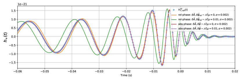
Figure 1: We show the time domain waveform in a signal frame (before projecting it in the detector) for one of the polarization $(+)$ for a GW150914-type signal. Apart from the reference waveform model IMRPhenomPv2 $h_{+,ref}^{SF}(t)$ (blue, denoted by ‘+’ markers), we also show the modification to the reference signal by one of the parametrizations described in the text. Red and violet waveforms represent the abs-phase modification given by (8). We use cubic splines for the parameters $(\delta\tilde{A},\delta\tilde{\phi})$ with a realization from the normal distribution as shown in corresponding plot legends. Orange and green waveforms represent the modification with rel-phase parametrization given by equation (9).

IV.1 GW waveform error parametrizations

In the present work, we use the following parametrizations to account for waveform modeling errors:

• abs-phase: Relative errors in amplitude and absolute errors in phase:

  $$\tilde{h}_{model} = \tilde{A}_{0}(1+\delta\tilde{A})\exp\{\iota(\tilde{\phi}_{0}+\delta\tilde{\phi})\},$$ (8)

  $$= \tilde{h}_{0}(1+\delta\tilde{A})\exp\{\iota\delta\tilde{\phi}\},$$

• rel-phase: Relative errors in amplitude and phase:

  $$\tilde{h}_{model} = \tilde{A}_{0}(1+\delta\tilde{A})\exp\{\iota\tilde{\phi}_{0}(1+\delta\tilde{\phi}_{\mathrm{rel}})\},$$ (9)

  $$= \tilde{h}_{0}(1+\delta\tilde{A})\exp\{\iota\tilde{\phi}_{0}\delta\tilde{\phi}_{\mathrm{rel}}\},$$

where $\tilde{h}_{0}=\tilde{A}_{0}\exp{(\iota\tilde{\phi_{0}})}$ represent the baseline (or reference) model, which aspires to be a ‘true’ model. However, as no waveform model is perfect to arbitrary accuracy, we introduce additional terms to account for potential systematics. $\delta\tilde{A}$ represent the fractional or relative error in the amplitude of the signal, and $\delta\tilde{\phi}$ ($\delta\tilde{\phi}_{\mathrm{rel}}$) represent absolute (relative/fractional) errors in phase. So, at the linear order perturbation, we can model the errors in the signal using relative or absolute errors in phase. The abs-phase parametrization described by Eq. (8) is also used in the correction for the detector calibration (to be discussed in the following subsection). Other studies also uses this parametrization to quantify the waveform uncertainties using parameters $\delta\tilde{A}$ and $\delta\tilde{\phi}$ (Edelman et al., 2021; Read, 2023). Since $\delta\tilde{A}$ is the relative change in amplitude, it is a dimensionless parameter in these parametrizations. The units of $\delta\tilde{\phi}$ is radian in abs-phase parametrization while $\delta\tilde{\phi}_{\mathrm{rel}}$ is a dimensionless parameter. From now on, we will drop the subscript ‘rel’ from the $\delta\tilde{\phi}$ parameter and we will refer these parameters as pair $(\delta\tilde{A},\delta\tilde{\phi})$, which in general are functions of frequency. The reader should pay attention to which parametrization we are talking about: abs-phase or rel-phase, and based on the parametrization, the meaning of these parameters will be adopted. We refer to these models as waveform error parametrization models or WF-Error parametrization for short.

The SNR (3) and the inner product (20) used in PE obey a symmetry between the observed data and the GW model. Therefore, if one accounts for calibration uncertainties in the data, this should have the same effect as accounting for waveform systematics. Since the calibration uncertainties are modeled with absolute errors in phase, marginalizing over calibration uncertainties can account for waveform systematics if they are of the same order. However, it is worth pointing out that all GW Transient Catalogs (GWTCs) included the effect of uncertain detector calibration in the analysis of GW events. Despite marginalizing over amplitude and (absolute) phase uncertainty for each detector, the properties of some binaries showed significant systematic differences between the waveform models that have been employed for the analysis (e.g., GW190412 Abbott et al. (2020b), GW191109_010717, GW191219_163120, GW200129_065458; see Sec. III E in Abbott et al. (2023b)). Evidently, marginalizing over calibration uncertainties did not incorporate all waveform systematics.

This is not unexpected. Systematic uncertainties in waveform models can often appear as secular phase drifts caused by numerical errors, (unavoidably) incomplete series expansions, interpolation inaccuracies, or even missing physics. The resulting waveform errors can, therefore, become much more severe than random small fractions of a radiant in the phase. If one wants to allow for possibly significant waveform uncertainties, large absolute phase errors must be considered, which may lead to an overly pessimistic error estimate. Alternatively, a small relative phase error is likely more appropriate to model systematic waveform uncertainties at the leading order. A relative error is well adapted to the parameter conventions used in the LIGO Algorithms Library Suite (LALSuite LIGO Scientific Collaboration (2018)), where a signal is typically defined with a set reference phase at the starting frequency. At this point, the phase error vanishes by definition. However, phase errors accumulate as the signal sweeps through the frequency band, which is well modeled by a relative phase error.

We now turn to incorporating WF-Error parametrizations in PE analysis. Ideally, a waveform model shall consist of the best-estimated reference model $\tilde{h}_{\mathrm{ref}}$, and priors for the parameters $\delta\tilde{A}$ and $\delta\tilde{\phi}$ for rel-phase or abs-phase parametrization to account for the waveform systematics. We call them WF-Error priors or error budget. The WF-Error priors should generally depend on the parameter space. We expect these priors to be narrower in the regime where many NR simulations are available, and waveform models are calibrated to greater accuracy. For the regions where NR simulations are sparse and theoretical waveform description is not so accurate, we expect them to be broader. For a given signal in parameter space, we also expect these priors to be broader for the frequencies close to the merger, where the analytical models extending from the inspiral regime to the merger are calibrated with NR simulations.

In the absence of such priors from the waveform modeling side, we can use a conservative approach and use wide enough priors so that we expect to capture any systematic and use data to constrain the parameters related to waveform errors. It might lead to broader posterior distribution resulting in larger variance on signal parameters (especially for weak signals), but it is expected to be unbiased. We will test these assumptions in the section VI with simulated signals and recovery.

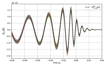
Figure 2: We show the time domain waveform for $(+)$ polarization for the GW150914 type signal. The reference waveform model IMRPhenomPv2: $\tilde{h}_{+,ref}^{SF}(t)$ is shown as dashed black curve. Other curves are modified waveform with abs-phase modification, described by equation (8), with WF-Error parameters sampled from the distribution $\delta\tilde{A},\delta\tilde{\phi}\sim\mathcal{N}(\mu=0,\sigma=0.05)$.

Figure 1 shows an example of waveform with GW150914 type signals and the modifications applied in the frequency domain using cubic splines (see Appendix A). To generate the reference signal, we use the IMRPhenomPv2 waveform model with source frame masses $(m_{1},m_{2})=(36M_{\odot},29M_{\odot})$ at the luminosity distance of 500 Mpc. We used non-spinning injections for this example. For the modifications, we use both the parametrizations described previously with WF-Error parameters chosen from a realization of the Normal distribution described in the figure. For the same values of $\delta\tilde{\phi}$, the rel-phase parametrization significantly modifies the reference model compared to abs-phase parametrization. In Figure 2, we show the reference waveform model for the GW150914 type signal described above along with the modified waveform curves with abs-phase modification. We use cubic splines with ten waveform nodal points in frequencies with values $(\delta\tilde{A},\delta\tilde{\phi})$ drawn from a normal distribution $\mathcal{N}(\mu=0,\sigma=0.05)$.

It is important to note that the WF-Error parametrizations (abs-phase and rel-phase) can be transformed into one another using simple mathematical relations by evaluating the phase $\tilde{\phi}_{0}$ of the reference waveform model $\tilde{h}_{\mathrm{ref}}$. We can use one of the parametrizations and mathematical transformations to convert it into the other according to the situation. However, using the correct parametrization is desirable for practical purposes in PE analysis. As an example, if the rel-phase parametrization is used for waveform systematics, and if one chooses abs-phase parametrization in PE, the priors for $\delta\tilde{\phi}$ need to become wider for larger frequencies to account for the growing reference phase $\tilde{\phi}_{0}$.

We can use hints from the mismatch (see Appendix B) studies to decide which WF-Error parametrization is better suited for practical purposes. In Figure 3, we show the distribution of mismatches between the reference waveform model and the modified one using both parametrizations. We use the Gaussian prior with zero mean and a fixed standard deviation across frequency range to generate the modified signal $h_{\mathrm{mod}}$. As expected, even with the narrower Gaussian prior, the rel-phase parametrization produces significant deviation to the $h_{\mathrm{ref}}$ compared to the abs-phase model, hence more significant mismatches. When we are in the parameter space where larger mismatches are expected, we can set our PE analysis framework to use rel-phase parametrization.

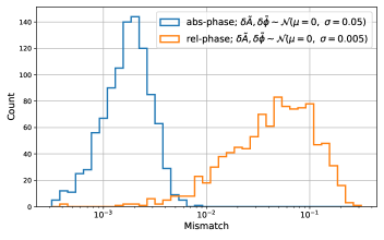
Figure 3: On the x-axis, we show the mismatch between the reference waveform model $h_{\mathrm{ref}}$ and the modified waveform model $h_{\mathrm{mod}}$. The modified signal, $h_{\mathrm{mod}}$, is generated by either abs-phase or rel-phase WF-Error parametrization. The WF-Error parameters are taken from the normal distribution, and we generate cubic spline curves to modify the reference model. The rel-phase model is generally well suited to model comparatively more significant mismatches.

IV.2 Calibration uncertainties

When GW passes through the detector, it produces a differential arm displacement between two L-shaped arms relative to the original arm lengths. This differential arm displacement generates laser power fluctuations in the photodetector, reproduced as the time series data. The conversion to the digital strain data regarding time series from the differential arm displacement happens through the control loop and calibration pipeline (Cahillane et al., 2017; Sun et al., 2020). The calibration of the strain data are modeled with systematic and statistical errors, which are then provided as calibration uncertainties as function of frequency (Sun et al., 2020, 2021; Cahillane et al., 2017; Acernese et al., 2022, 2018). Figure 4 shows the calibration envelopes for the LIGO-Hanford detector around the event GW150914.

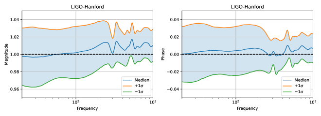
Figure 4: The Figure shows the calibration uncertainties as a function of frequency for the LIGO Hanford detectors around the time of the first GW detection: GW150914. The left panel shows the systematic error in the magnitude, while the right panel shows the systematic error in the phase angle (in radians). The shaded region represents the $\pm 1\sigma$ band around the median systematic error. The systematic error is described by the ratio of the true response function to the modeled response function of the detector. The LIGO and Virgo calibration uncertainty files for O1, O2, and O3 observation runs are available at (lig, ).

The calibration uncertainties are modelled as frequency dependent errors in phase and amplitude as follows (Farr et al., 2015; Cahillane et al., 2017):

$$\tilde{h}_{\mathrm{obs}}=\tilde{h}_{\mathrm{true}}(1+\delta\tilde{A}_{cal})\exp{(\iota\delta\tilde{\phi}_{cal})},$$ (10)

In terms of the general parametrization we discussed above, $\delta\tilde{A}_{cal}$ can be identified as relative error in amplitude while $\delta\tilde{\phi}_{cal}$ is absolute error in the phase. In the calibration uncertainty model, equation (10), the exponential term can be expanded as a Taylor series and is rewritten as,

$$\tilde{h}_{\mathrm{obs}}=\tilde{h}_{\mathrm{true}}(1+\delta\tilde{A}_{cal})\frac{2+\iota\delta\tilde{\psi}_{cal}}{2-\iota\delta\tilde{\psi}_{cal}},$$ (11)

where the ratio involving $\delta\tilde{\psi}$ is chosen in such a way that it always have the complex amplitude of one, which makes it purely the phase shift (Farr et al., 2015).

V Fisher Matrix Estimates For Biases

A standard tool in the literature to quantify systematic errors between two waveform models is the Fisher matrix formalism Dhani et al. (2024b); Dupletsa et al. (2024). In this section, we will apply it to see how significantly errors modelled as (9) change the recovery of source parameters $\Theta^{\mu}$. An introduction to the Fisher matrix formalism is provided in appendix B. A reader who is familiar with these topics may skip this section and move directly to the section VI.

V.1 Setup of the analysis

In this part, we introduce methods to test how well the Fisher estimates work in trying to recover biases induced by certain choices of $\delta\tilde{A},\delta\tilde{\phi}$. We do that by performing two sets of PE runs for each combination of $\delta\tilde{A},\delta\tilde{\phi}$: (i) where the data are a zero-noise injection generated from the signal model (9) for the chosen values $\delta\tilde{A},\delta\tilde{\phi}$; (ii) where the data are the same baseline signal (in zero noise), but now generated with $\delta\tilde{A}=\delta\tilde{\phi}=0$, i.e. without any error model. The results of run (ii) can thus be seen as a reference for the results of run (i). In all cases the same waveform model is used, the signal models only differ in the error model used. These PE results are then taken as a reference for the Fisher estimates and used to validate them. If we were to work with just Fisher estimates, only the results from run (ii) would be required as they already yield a point in which the relevant formulas can be evaluated. However, having a reference is very valuable because the estimates are subject to some uncertainty due to the approximations involved (most notably, the LSA (24)).

The recovery is always performed using the baseline waveform model, which corresponds to a recovery using the signal model (9) with $\delta\tilde{A}=\delta\tilde{\phi}=0$. The injection parameters chosen for these analyses are quoted in table 1. We keep the extrinsic parameters $\psi,\alpha,\delta$ fixed and vary mainly the ones in signal frame, namely $\mathcal{M},q,D_{L},\iota$ (our focus is on non-spinning binaries). Applying the alignment procedure then requires to also take time, phase shift into account. Both of them are also standard parameters included in PE, corresponding to the time of arrival $t_{c}$ and a global phase $\phi_{0}$.

In the end, the set of parameters constituting the Fisher matrices we calculate is

$$\{\mathcal{M},q,D_{L},\iota,t_{c},\phi_{0}\}\,.$$ (12)

which is also the set of parameters varied during the PE runs. We are aware of results in the literature that have shown that the interplay of $D_{L},\iota$ can lead to problems with Fisher matrix estimates. To make sure our conclusions are robust against this issue, we have repeated all calculations without these two parameters. The results showed that including or excluding $D_{L},\iota$ did not have a strong impact on our conclusions and therefore, we have decided to use (12).

fisher_signal_params

Table 1: Injection Parameters for the base signal. In the high-SNR case, the luminosity distance is changed, now taking a value of $100\,\mathrm{Mpc}$ instead and accordingly, the SNR changes to $83.91$. Note that the SNR values quoted here refer to the non-modified injection, for the modified one the SNR will be slightly different (with deviations being on the order of $1\%$).
We use priors that are uniform in component mass for $\mathcal{M}^{\mathrm{z}},q$, uniform in $\cos(\iota)$ for the inclination (i.e. $p(\iota)\propto\sin(\iota)$), uniform in comoving volume for the luminosity distance, and uniform in coalescence time $t_{c}$ (no prior for $\phi_{0}$ because we use a marginalized-phase likelihood).

fisher_results

Table 2: Summary of results from full PE runs and Fisher matrix estimates. The numbers one should primarily compare the neighbouring columns labeled ”PE” and ”Fisher”, for each of the four quantities that appear in the upper row. Moreover, when comparing them one should keep in mind that neither number is expected to be perfectly accurate, explaining certain small deviations; PE results are always subject to sampling uncertainties, while limitations of the Fisher approach have been laid out at the beginning of this section.

There are two properties of the posteriors that we wish to compare to the respective Fisher matrix estimate:

1. First of all, the systematic error $\Delta\Theta^{\mu}$. From (21) we see that it is formally defined as the difference between maximum a posteriori estimate $\Theta_{\mathrm{bf}}$ and true parameters $\Theta_{\mathrm{tr}}$. Therefore, it is natural to calculate it as the difference of the maximum of the posterior recovered from the modified injection and the respective injected value, for each parameter of interest. We do expect that this should be equivalent to taking the difference between the maxima of the recovery of modified and non-modified signal, and have verified that this is indeed the case, up to the accuracy expected when taking sampling effects into account.

   In practice, however, we do not compute the actual maximum of each marginalized posterior. Instead, following the method chosen in gravitational-wave transient catalogs Abbott et al. (2019b, 2021c); The LIGO Scientific Collaboration et al. (2021b, a), we use the posterior medians. This number is less susceptible to sampling effects and in the limit of Gaussian posteriors (the validity of which we rely on anyway when applying Fisher matrix tools) even equal to the maximum.

2. Secondly, the posterior width. As Ref. Vallisneri (2008) shows, in the linear-signal regime (i.e. in particular in the high-SNR limit) the standard deviation of the statistical bias (when varying the noise realization) is nothing but the standard deviation of the posterior itself. The latter can thus be estimated as (cf. (23))

   $$\sigma_{\Theta^{\mu}}\simeq\sqrt{(\Gamma^{-1})^{\mu\mu}}$$ (13)

   and this number is compared to the standard deviation of the marginalized posterior for $\Theta^{\mu}$.

V.2 Results of comparing Fisher matrix estimates with PE runs

In total, we have analysed four scenarios: two different sets of error values of $\delta\tilde{A}=0.004,\delta\tilde{\phi}=0.004$ and $\delta\tilde{A}=0.01,\delta\tilde{\phi}=0.01$, and for each of them one moderate- and one high-SNR case (cf. table 1). All of the signals have been injected as a zero-noise injection into the Hanford detector with an O4 PSD. The results are summarized in table 2, with a visualization provided in the appendix (Fig. 14).

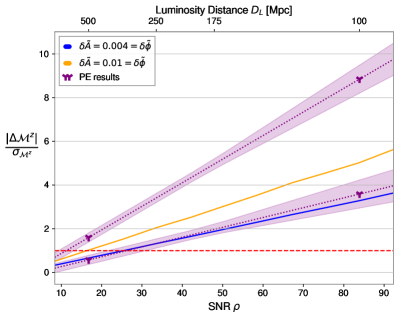
(a)  rel-phase Parametrization

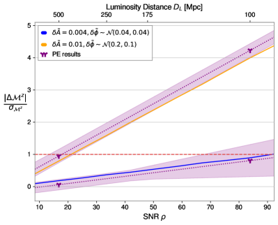
(b)  abs-phase Parametrization

Figure 5: Evolution of the bias ratio $\frac{|\Delta\mathcal{M}^{z}|}{\sigma_{\mathcal{M}^{z}}}$ as a function of the SNR $\rho$, for both error models rel-phase and abs-phase. The blue and orange lines are obtained from Fisher estimates, while the purple triangles in (a) represent PE results (the rel-phase ones of which have been discussed in this section). The dashed, purple lines and shaded regions represent a fit of the PE results and corresponding uncertainties, which serves as a comparison and reference for the Fisher matrix results. Details on how we obtain the uncertainty bands are discussed in appendix B.1. The red, dashed line marks $|\Delta\mathcal{M}^{z}|=\sigma_{\mathcal{M}^{z}}$, i.e. the point where bias hierarchy switches. In addition to the SNR values, we also show the $D_{L}$ values they correspond to on the top axis. For the absolute error in (b), we do not use a constant shift since this is easily captured by phase marginalization in the PE case and the alignment procedure for the Fisher estimates, resulting in no net bias for $\mathcal{M}^{z}$. Instead, we draw random samples at fixed nodal points, a technique that is discussed more thoroughly in subsection VI.2. The induced randomness will lead to some remaining imprint of the abs-phase model and thus some bias even after marginalization, alignment.

Since the chosen signal lies in the non-spinning part of the parameter space, the remaining intrinsic parameters are the masses parametrized by the tuple $\mathcal{M}^{\mathrm{z}},q$. We will direct our attention toward these two, not discussing biases in the luminosity distance $D_{L}$ and inclination $\iota$ in detail. This is because the uncertainty in $D_{L}$ is typically very large. Moreover, there is a known correlation between these two parameters, which makes their recovery and the assessment of their bias results more complicated.

The first important finding is that the PE results are biased if a modified signal is recovered using the baseline, non-modified model. This finding implies that the error model (9) is capable of parametrizing systematic errors in the way we intend it to. Moreover, we find that these biases can be recovered in the Fisher matrix framework, validating that the biases have a physical origin rather than being an artifact of flawed application of PE or an error in the implementation. The statistical bias in particular is recovered very well in all four scenarios, whereas this statement does not generally hold true for the systematic bias (cf. the values in table 2). For the two configurations with smaller waveform errors ($\delta\tilde{A}=\delta\tilde{\phi}=0.004$), all biases are recovered reasonably well. The seemingly large discrepancy between real and estimated $\Delta q$ for the base signal case can very likely be attributed to sampling effects, as the difference between unbiased recovery and injected value take the almost identical value of $-0.018$ (not shown in the table). Moreover, $\Delta q$ is still clearly subdominant to the width $\sigma_{q}$, so that our conclusion of numbers being well recovered stands.

Those results motivate the following interpretation: in case of $\delta\tilde{A}=\delta\tilde{\phi}=0.004$, the waveform differences introduced into the waveform are still well approximated by the linear expansion (24), the LSA is justified; this clearly changes for $\delta\tilde{A}=\delta\tilde{\phi}=0.01$, where the systematic bias estimates begin to diverge from the corresponding PE results – the LSA is not a faithful approximation anymore. For the chirp mass, it is just the magnitude of the value that is off by factor of $\sim 2$, with the sign ($\equiv$ direction of the error) being correct. That, however, corresponds to the estimate being off by a full standard deviation, which is certainly too large to still be considered a faithful approximation. Furthermore, for the mass ratio both magnitude and direction do not match the result obtained from the full PE run. Sampling effects do not seem to be a suitable explanation for this because, although the order of magnitude is the same for the deviation we observe between injected value and median of unbiased recovery, the actual value of $\Delta q$ in table 2 is still about $3$ times higher. Additionally, the latter argument can certainly not be applied to the high SNR case, where such biases are present too.

As already mentioned briefly, the statistical bias agrees well for all runs, with differences being on the order of the second significant digit. This agreement is a very interesting feature of the results because it indicates that the statistical bias estimate (23) seems to be more robust to increasing waveform differences and thus potential violations of the LSA than the systematic bias estimate (21) (at least for our applications).

V.3 Implications

We have seen that Fisher estimates can work, but not always. What does this mean for us and our objectives? First of all, it was expected that the LSA will not hold up to arbitrarily large values of $\delta\tilde{A},\delta\tilde{\phi}$, simply because we use the relative error model where errors accumulate from low to high frequencies and thus will quickly result in large waveform differences. However, this being the case for a $1\%$ error has serious implications for a practical application of the Fisher estimates: for realistic scenarios, where errors of this magnitude are expected, they are not suitable. Of course, in other parts of the parameter space, other thresholds for the LSA validity might exist, but the existence of such a counterexample in a part of the parameter that is certainly relevant for detected signals is already sufficient to recognize that we should not rely on a faithful estimation of biases. The numbers are particularly concerning for the high-SNR signal with $\delta\tilde{A}=\delta\tilde{\phi}=0.01$ since this corresponds to the to data from next-generation(GW detectors, where a tenfold increase in sensitivity is aimed for. Here, Fisher estimate and true recovery are basically fully separate (cf. Fig. 14). All of this plays into why we choose to not use Fisher matrix estimates for the rest of this paper. A suitable replacement to still account for these systematic errors by using waveform with an error model like (9) on top of them is discussed in the next section.

That being said, there is still a role to play for Fisher estimates. Even though they might lack the ability to precisely estimate biases for arbitrary values of $\delta\tilde{A},\delta\tilde{\phi}$, they typically estimate the correct order of magnitude, being off by a factor of $\sim 2$, and reproduce the statistical bias very well. Therefore, it is usually possible to make a statement on the hierarchy of the two errors, thereby assessing the need to account for waveform errors. In that case, it would be possible to use the results of a PE run performed without accounting for them and then assess the need to incorporate them using Fisher matrix estimates. This would be advantageous since it would save the additional computational cost involved in sampling more parameters related to $\delta\tilde{A},\delta\tilde{\phi}$, if it is not strictly necessary. Since we anticipate values (or at least estimates) for $\delta\tilde{A},\delta\tilde{\phi}$ would be given for realistic applications, we would know in advance whether Fisher estimates can be trusted for these values or not. For the specific point in parameter space that we have looked at here, the threshold is right around the first configuration with $\delta\tilde{A}=\delta\tilde{\phi}=0.004$. We acknowledge that these values will most likely vary throughout the parameter space, but through careful analysis it would be possible to find analogous thresholds.

A practical usage of the method presented in this paragraph could then involve looking at curves like the ones shown in Fig. 5, where the bias ratio $|\Delta\mathcal{M}^{z}|/\sigma_{\mathcal{M}}^{z}$ is plotted as a function of the SNR $\rho$. A detailed description is given in the corresponding caption, but the bottom line is that such a plot encapsulates the significance of expected biases. Not surprisingly, in the rel-phase configuration of Fig. 5 (a), this works much better for the configuration with $\delta\tilde{A}=\delta\tilde{\phi}=0.004$ (since the corresponding solid line lies within the shaded uncertainty band), where the LSA still seems to be justified, whereas the ‘non-LSA’ one with $\delta\tilde{A}=\delta\tilde{\phi}=0.01$ exhibits larger deviations between PE results and Fisher estimates (which is consistent with the previous findings from this section). For the abs-phase results shown in Fig. 5, the results for both configurations are recovered well by Fisher matrix estimates. Here, the search for a ‘non-LSA’ configuration is complicated by the fact that any constant absolute shift in $\delta\tilde{\phi}$ will be corrected for by the procedures alignment, marginalization we use for Fisher estimates, PE, respectively. Consequently, the mean of $0.2$ is not the quantity of interest here and it is only the standard deviation $\sigma$ that really matters. Evidently, even a value of $\sigma=0.1$ does not lead to ‘non-LSA’ configuration (which could be explained by the inherent randomness of the configuration we draw from this distribution). However, this result is actually very advantageous for what Fig. 5 was intended for: it allows us to assess the point at which systematic biases become dominant more accurately, even for what we would consider large biases (‘large’ in the abs-phase parametrization; when compared to typical phase offsets generated by the rel-phase parametrization, on the other hand, these values would presumably not be considered large).

In case we are unable to find suitable thresholds, there are two scenarios that can occur in case of inaccurate Fisher estimates, and we discuss them here for completeness: (i) a false alarm, where the systematic bias appears to be larger than the statistical one, even though it is actually smaller; (ii) a false dismissal, where the systematic bias appears to be smaller than the statistical bias, although it is larger. We have seen an example of a false alarm in the estimate of the mass ratio bias for the ‘non-LSA’ configuration with $\delta\tilde{A}=\delta\tilde{\phi}=0.01$. In a hypothetical practical application, this case would trigger a follow-up PE run with an error model like (9), where it would be revealed that the actual bias is much smaller. Consequently, (i) would not prohibit us from making the best possible recovery of the source parameters. A false dismissal, on the other hand, would be more concerning. In that case, no follow-up PE run would be launched and a potentially biased result would be taken as the truth. For this reason, a robust way of assessing the reliability of Fisher estimates would be crucial for its role as an alert tool to work.

VI Simulations and Tests of Parameter Estimation Framework

This section uses simulations to test the WF-Error parametrizations described in section II. Though we do not have access to the ‘true’ waveform model, we can still check the validity of the PE framework we describe by considering a reference waveform model, $h_{\mathrm{ref}}$, modifying the $h_{\mathrm{ref}}$, and checking if our parametrization can pick up the introduced modification. We take a reference signal $h_{\mathrm{ref}}$ described by a waveform approximant and introduce errors in the model described by parametrizations in equations (8) and (9). Now we have a modified signal $h_{\mathrm{mod}}$, which shall have a systematic error compared to the $h_{\mathrm{ref}}$. We consider $h_{\mathrm{mod}}$ as the ‘true’ signal and inject it in the strain data of LIGO detectors at Hanford (H1), Livingston (L1), and Virgo detector (V1). Then, we use the Bayesian PE data analysis pipeline to recover the source properties using $h_{\mathrm{ref}}$ as our waveform model with and without incorporating waveform uncertainties in PE. In order to separate the effects of waveform systematics and other effects, we consider non-spinning signals for all the simulations. In the subsequent subsections, we describe each injection-recovery campaign’s injected signals and PE scheme.

Recovery Model	Sampling Parameters	Description	Prior
IMRPhenomPv2	$\mathcal{M}$	Source frame chirp mass	Uniform in component masses
	$q=\frac{m_{2}}{m_{1}}~(m_{1}\geq m_{2})$	Mass ratio
	$V_{c}$	Comoving volume	Uniform: $\pi(V_{c})=\mathcal{U}(5\times 10^{3},9\times 10^{9})$
	$\iota$	Inclination angle	$\pi(\iota)\propto\sin(\iota)$
	$t_{c}$	Time of arrival	Uniform: $\pi(t_{c})=\mathcal{U}(t_{c}-0.1,t_{c}+0.1)$
	RA, dec	Right ascension and declination	Uniform Sky
	$\psi$	Polarization Angle	Uniform angle: $\pi(\psi)=\mathcal{U}(0,2\pi)$
IMRPhenomPv2 + WF Error	$\delta A_{i},\delta\phi_{i}$	WF-Error parameters	$\mathcal{N}(\mu=0,\sigma=0.032)$

Table 3: This table describes the priors used in the PE of simulated signals. The distribution $\mathcal{U}(a,b)$ refers to a one-dimensional uniform distribution defined within the interval $(a,b)$. For the WF-Error parameters, when we employ cubic spline curves with ten nodal points across the frequency range of $(20,500)$ Hz. The prior distributions for each $\delta\tilde{A}_{i}$ and $\delta\tilde{\phi}_{i}$ are specified accordingly. The same prior is used for the special test cases, when we do not use cubic spline but a constant shift in amplitude and phase with parameters $\delta\tilde{A},\delta\tilde{\phi}$. $\pi(\theta)$ denotes the prior distribution used for a parameter $\theta$

.

For PE, we use the publicly available toolkit PyCBC Inference (Biwer et al., 2019), and for sampling the likelihood function, we use the nested sampling algorithm implemented in the publicly available code Dynesty (Speagle, 2020). We also implement WF-Error parametrizations in code that serves as a plugin (Kumar et al., 2025) for PyCBC. We use the aLIGOZeroDetHighPower PSD for the LIGO Hanford and Livingston detectors and the AdvVirgo PSD for the Virgo detector. These PSD functions are implemented in publicly available modules LALSimulation, which is a part of the LALSuite code (LIGO Scientific Collaboration, 2018). We use two sets of runs for each injection:

• In first set of run, we sample the parameter space with the following parameters: source frame chirp mass ($\mathcal{M}$), mass ratio $q(q=\frac{m_{1}}{m_{2}},m_{1}\geq m_{2})$, comoving volume, inclination angle, and geocentric time of arrival of the signal ($t_{c}$). We fix right ascension (RA), declination (dec), and polarization angle ($\psi$) for these runs.

• In the second sets of runs, in addition to the parameters described above, we also vary ra, dec, and $\psi$.

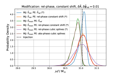
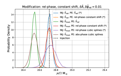
Figure 6: Injection and recovery are shown for a non-spinning GW150914-like signal with source frame masses $(m^{src}_{1},m^{src}_{2})=(36,29)~M_{\odot}$, at a luminosity distance of 500 Mpc (left panel) and a distance of 100 Mpc (right panel). We also inject a modified signal with rel-phase modification with parameters $(\delta\tilde{A},\delta\tilde{\phi})=(0.01,0.01)$. When we inject a modified signal and use the incorrect model to recover, we see a bias in the recovery of detector frame chirp mass $\mathcal{M}^{\mathrm{z}}$. We also show that using the correct parametrization (in this case, rel-phase) can correct the bias and get a broader marginalized posterior sample. The bias is more prominent in a louder signal (right panel) than in a comparatively weaker signal (left panel). We mark that combination of injection and recovery by an asterisk ($\star$) where we do not expect a bias. The verticle dashed line represents the injected value of $\mathcal{M}^{\mathrm{z}}$. For these PE runs, we fix the parameters RA, dec, and polarization to the injected values.

We transform the sampling parameters to the waveform model parameters, such as detector frame masses ($m_{1}^{\mathrm{z}},m_{2}^{\mathrm{z}}$ ), and luminosity distance ($D_{L}$) through standard transformations. We fix the spins to be zero for the study in this manuscript, except for in sub-section VI.3. For the PE runs described by WF-Error parametrizations, we use additional parameters. We use two additional WF-Error parameters for the constant shift models: $\delta\tilde{A}$ and $\delta\tilde{\phi}$. For the cubic-spline model, we use ten frequency nodal points with log spacing between a minimum frequency of 20 Hz and a maximum frequency of 500 Hz.

In Table 3, we describe the prior distribution for each of the abovementioned parameters. All the injections described in this section are zero-noise injections.

VI.1 Simplest modification: A constant shift in amplitude and phase

We consider a GW1500915-like signal with source frame masses $m_{1},m_{2}=(36~M_{\odot},~29~M_{\odot})$ at a distance of 500 Mpc. We generate the corresponding reference signal using the IMRPhenomPv2 waveform model and introduce the errors in reference signal with rel-phase parametrization corresponding to:

$$(\delta\tilde{A},\delta\tilde{\phi}_{\mathrm{rel}})=(0.01,0.01)$$ (14)

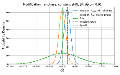
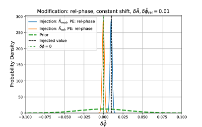
Figure 7: Recovery of the parameter $\delta\tilde{\phi}$ for rel-phase parametrization for various scenarios of injected parameters. The signal injected here is a non-spinning GW150914-like, as in Figure 6. The left panel has an injection at 500 Mpc, while the right panel shows the case with an injection at 100 Mpc. The verticle dashed line shows the injected value for $\delta\tilde{\phi}$ for the modified signal. The green dashed curve shows the prior distribution for the $\delta\tilde{\phi}$ parameter. We can recover the injected value of $\delta\tilde{\phi}$ with the correct parametrization for PE. We recover $\delta\tilde{\phi}=0$ for the reference injection. For these PE runs, we fix the parameters RA, dec, and polarization to the injected values.

For this most straightforward case, a constant phase shift is expected to be significant for rel-phase parametrization. For abs-phase parametrization, a constant phase shift will not introduce any physical effect except a constant shift in time. We will consider the general modification with abs-phase parametrization in the following subsections. We perform PE with the injected signal in the detector network, HLV, with the following combination:

• Injection: standard, PE: standard In this scenario, we inject the reference signal as described above and perform the PE with the same waveform model without introducing the WF-Error parametrization.

• Injection: modified, PE: standard In this scenario, we inject the modified signal and perform the PE with the reference waveform model without introducing the waveform errors.

• Injection: modified, PE: WF-Errors In this scenario, we inject the modified signal, perform the PE with the reference waveform model + WF-Error paramtrization.

• Injection: standard, PE: WF-Errors Here, we inject the reference signal, perform the PE with the reference waveform model+WF-Error.

In Figure 6, we show the injection and recovery of various combinations. We show that when we have a modified injection (equivalent to a systematic error with rel-phase parametrization), and we perform PE with reference waveform model, we get a bias in the detector frame chirp mass $\mathcal{M}^{\mathrm{z}}$. This bias is corrected when we use the right parametrization to account for waveform systematics. We also note that we can correct the bias when we use cubic splines for constant shift error in the reference signal. However, it is to be noted that when we use abs-phase parametrization to correct for the bias introduced by rel-phase parametrization, it fails to correct for the bias. These effects are more visible in a louder signal, which is simulated by injection at a closer luminosity distance (100) Mpc compared to one at 500 Mpc. Figure 7 shows the recovery of parameter $\delta\tilde{\phi}$ with rel-phase parametrization. We show that we can recover the injected value of $\delta\tilde{\phi}$ with the correct parametrization. When there is no modification to the reference signal, the rel-phase parametrization recovers $\delta\phi=0$. We fix the RA, dec, and $\psi$ for the runs shown in figures 6 and 7. We find that the $\delta\tilde{A}$ parameter returns the prior distribution and does not have a constraining power for the PE runs described in this subsection. For simplistic cases, we expect $\delta\tilde{A}$ to be degenerate with distance, i.e., a small constant shift in the amplitude can be modeled in the luminosity distance. At this stage, it can be argued that we can get rid of $\delta\tilde{A}$ parameter in the WF-Error parametrization and focus on $\delta\tilde{\phi}$ parameter. However, we shall keep this parameter in our model for more general scenarios where errors in amplitude can be a function of the frequency.

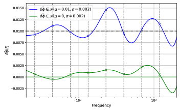
Figure 8: We show a realization of cubic spline curves with ten frequency nodal points (vertical dashed curves) for $\delta\tilde{\phi}_{i}$ taken from two normal distributions: one with zero mean (green curve) and the another with non-zero mean $\mu=0.01$ (blue curve). The points marked with a cross (x) are the realization of the normal distribution. In reality, these curves will represent a general function of frequency that captures the waveform systematics or deviation from the ‘true’ waveform model.

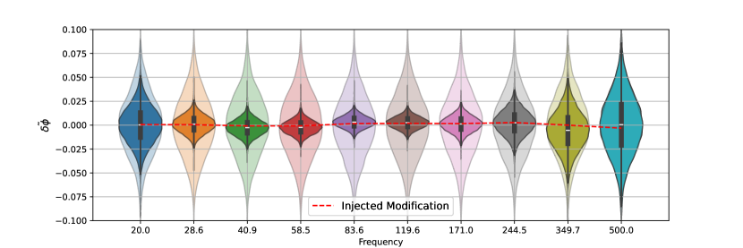
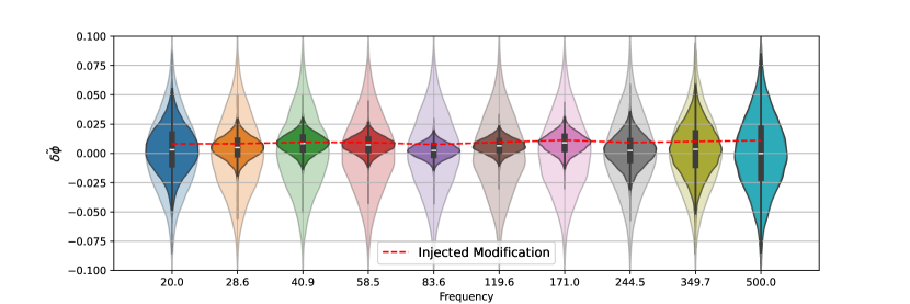
Figure 9: The recovery of WE-Error parameter $\delta\tilde{\phi}_{i}$ for rel-phase parametrization is shown for each frequency nodal point used in PE. The light violin plot represents the prior distribution for each $\delta\tilde{\phi}_{i}$, and the dark-shaded region represents the one-dimensional marginalized posterior samples. The last frequency nodal point at f=500 Hz returns the prior because the signal merges before this frequency. The constraints are also weaker at $f_{i}=20$ Hz because this frequency bin’s signal-to-noise ratio is comparatively low. a) The modification to the reference waveform is applied using the rel-phase parametrization with a cubic spline realization generated from the distribution $\delta\tilde{A}_{i},\delta\tilde{\phi}_{i}\sim\mathcal{N}(\mu=0,\sigma=0.002)$. Panel b) represent the modification from the distribution $\delta\tilde{A}_{i},\delta\tilde{\phi}_{i}\sim\mathcal{N}(\mu=0.01,\sigma=0.002)$. The GW150914-like signal is placed at a luminosity distance of 500 Mpc for both panels. For these PE runs, we fix the parameters RA, dec, and polarization to the injected values.

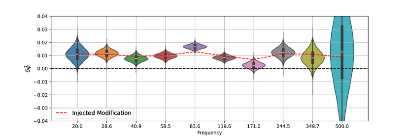
Figure 10: The recovery of WE-Error parameter $\delta\tilde{\phi}_{i}$ for rel-phase parametrization is shown for each frequency nodal point used in PE. The modification to the reference waveform is applied using the rel-phase parametrization with a cubic spline realization generated from the distribution $\delta\tilde{A}_{i},\delta\tilde{\phi}_{i}\sim\mathcal{N}(\mu=0.01,\sigma=0.002)$. For this particular example, the GW150914-like signal is placed at the luminosity distance of 100 Mpc. Since it is a comparatively loud signal, we observe that the recovery posterior samples at each frequency nodal point or knot follow the injected modification shown by the dashed red line. For this PE run, we fix the parameters RA, dec, and polarization to the injected values.

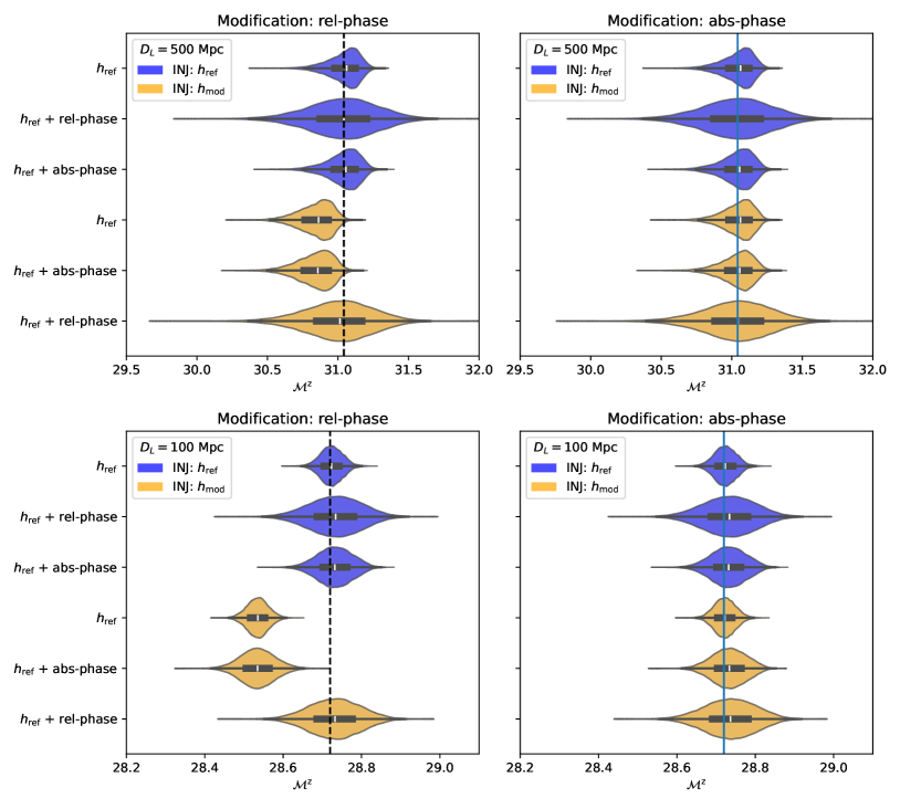
Figure 11: A GW150914-like signal is injected and recovered using two WF-Error formalisms. The blue violin plots show the cases with reference injection $h_{\mathrm{ref}}$ while orange violin plots show the modified injections. The left panels represent the cases where the modification is done with rel-phase modification, while the right panel shows abs-phase modification. The top rows represent the injections with the source placed at a luminosity distance of 500 Mpc, while the bottom panels show the injection corresponds to the same source placed at 100 Mpc. Labels on the y-axis show the waveform models used in PE runs. For these PE runs, we fix the parameters RA, dec, and polarization to the injected values.

Through these simulations, we have established that for a simplistic model, a systematic error corresponding to $\delta\tilde{\phi}=0.01$ can lead to significant bias in the detector frame chirp mass for GW150914-type signal, with the detector sensitivity of advanced LIGO design sensitivity. We have also shown that, by using WF-Error parametrization, we can account for the systematic errors introduced in the reference waveform. We can also recover the injected modification in the $\delta\phi$ parameter with correct parametrization. However, when we modify the reference waveform with rel-phase parametrization, the PE recovery with abs-phase parametrization fails to correct the observed bias in $\mathcal{M}^{\mathrm{z}}$. This is because the relative-phase parametrization can accommodate more significant deviations in the reference waveform than the absolute-phase parametrization for the same range of priors in $\delta\tilde{\phi}$, as previously discussed.

VI.2 A more realistic modification using cubic splines

Within the framework of WE-Error parametrizations, a waveform model $h_{\mathrm{ref}}$ will deviate from the ‘true’ model described by general functions of frequency: $\delta\tilde{A}(f),\delta\tilde{\phi}(f)$. We use cubic splines to generate them at specific frequency nodal points. In this subsection, we introduce a more general type of modification to our reference GW150914-like signal within the framework of both the parametrizations:

$$\delta\tilde{A},\delta\tilde{\phi} \sim \mathcal{N}(\mu=0,\sigma=0.002)$$ (15)

$$\delta\tilde{A},\delta\tilde{\phi} \sim \mathcal{N}(\mu=0.01,\sigma=0.002)$$ (16)

Figure 8 shows examples of cubic spline curves generated from the abovementioned distributions. We use a realization of $(\delta\tilde{A}_{i},\delta\tilde{\phi}_{i})$ at nodal frequency points generated from the distributions described by the equations (15) and (16).

In Figure 9, we show the recovery of $\delta\tilde{\phi}$ parameter at each frequency nodal point for the modified injection generated using rel-phase parametrization. We demonstrate that the WF-Error parametrization framework can recover the $\delta\tilde{\phi}$ curves used to modify the reference waveform model. In another example (see Figure 10), for a source located at $D_{L}=100$ Mpc correspond to a loud signal, we observe that the posterior samples at nodal points align with the injected values of $\delta\tilde{\phi}$. These examples demonstrate that if the reference waveform model deviates from reality, which is described by rel-phase parametrization, the framework presented here has the potential to account for that. In other words, in the absence of true knowledge of WF-Error priors, we can use a data-driven approach to determine if there is a deviation from the reference waveform model, especially for loud signals.

We now focus on the other parameters, such as chirp mass $\mathcal{M}$. In Figure 11, we present various combinations of injections and PE recovery. Our findings can be summarized as follows:

• When the injection uses the reference waveform model $h_{\mathrm{ref}}$ and PE recovery is performed with the same model, we achieve the expected recovery with no bias.

• If we enable the waveform error parameterizations (rel-phase or abs-phase) while using the correct recovery model, we observe a broadening of the posterior samples as anticipated. The broadening of the posterior distribution is more pronounced with the rel-phase parameterization than the abs-phase parameterization.

• In the scenario when the injection is performed by modifying the reference signal and we use the reference signal to recover the source parameters, we get bias in the chirp mass. As expected, the bias is more prominent for a large SNR signal.

• In the case of modified injections, using WF-Error parametrization in conjunction with the $h_{\mathrm{ref}}$ recovery model broadens the posteriors. Additionally, employing the correct parametrization leads to a correction in bias. The bias introduced by rel-phase parametrization can only be corrected using rel-phase parametrization. The abs-phase parametrization does not correct the biases introduced by rel-phase parametrization.

• For the abs-phase parametrization, the moderate deviation introduced by the cubic spline curves generated from the abovementioned distribution does not introduce significant bias for a GW150914-like signal with advanced LIGO detector sensitivity. In order to see any significant bias for abs-phase parametrization, we either need a comparatively large deviation in phase or a very high SNR, such as in the case of 3G detectors.

Through these simulations, we conclude that if the ‘true’ waveform (WF) model deviates from the reference waveform model in a manner described by the parametrizations in equations (8) and (9), our framework can correct any bias in source parameters, if present. Additionally, a sufficiently loud signal can recover the frequency dependence of WE-Error parameters. We still need to ensure that the priors are sufficiently broad to capture the deviations. Additionally, the selection of knots or nodal points for cubic splines should accurately reflect the true nature of $\delta\tilde{\phi}$ as a function of frequency. In these examples, we use binning in log frequency and use a total of ten nodal points between 20 Hz and 500 Hz.

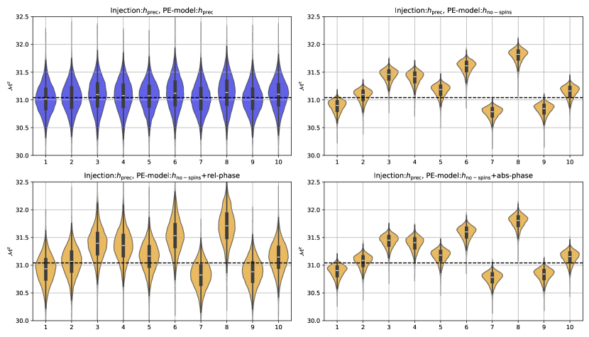
Figure 12: We use ten precessing injections in the HLV network. The top left panel shows the posterior samples from each PE run where we use the precessing recovery model: $h_{\mathrm{prec}}$. We use the nonspinning model $h_{\mathrm{no-spins}}$ for PE in the top right panel. The bottom panels use a nonspinning model along with the WF-Error framework. The bottom left plot shows recovery with rel-phase parametrization, and the bottom right model uses abs-phase parametrization. The horizontal dashed line represents the injected chirp mass ($\mathcal{M}^{\mathrm{z}}$) value in the detector frame. X-axes represent the injection simulation IDs. We use all the parameters listed in Table 3 for these PE runs. We also use component spin parameters $s_{1,2}^{x,y,z}$ for the precessing recovery.

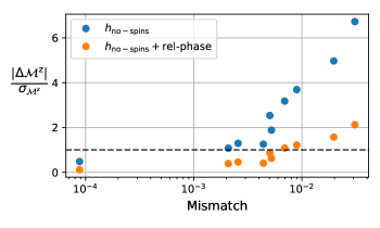
Figure 13: For the injections and recovery shown in Figure 12, on the x-axis, we show the mismatch between the waveform generated with non-spinning and precessing parameter values. We kept all other parameters the same (see text). The y-axis shows the ratio of the absolute value of the bias ($\Delta\mathcal{M}^{\mathrm{z}}=\mathcal{M}^{\mathrm{z}}_{median}-\mathcal{M}^{\mathrm{z}}_{inj}$) to the standard deviation of the 1D marginalized posterior samples of $\mathcal{M}$. Horizontal dashed line represent the the line where $\Delta\mathcal{M}^{\mathrm{z}}=\sigma_{\mathcal{M}^{\mathrm{z}}}$.

VI.3 Incorporating missing physics

One use of WF-Error parametrization can be to account for the missing physics. For BBH mergers, the most up-to-date waveform model includes effects such as higher-order harmonics and system precession, and the waveform developers are working on systems with eccentricity (Paul and Mishra, 2023; Henry and Khalil, 2023; Ramos-Buades et al., 2022; Paul et al., 2024). The most general description of a BBH merger can include other environmental effects such as matter accretion, another binary or heavy object nearby, or a merger near a supermassive BH near the host galaxy’s center.

However, the waveform model used in PE might not fully describe the reality. We want to see if the WF-Error parametrization can capture the deviation from the actual model because the missing effects are not considered in the waveform model. It is expected to come at the cost of measuring other known parameters in the model. In order to test this scenario, we injected a set of precessing signals with components coming from the uniform distribution $s_{1,2}^{x,y,z}\in\mathcal{U}(-0.1,0.1)$. We use the IMRPhenomPv2 model and other parameters described in the previous section. We call the injected model $h_{\mathrm{prec}}$. We expect bias in the measured parameters for a precessing injection if we use a recovery model that does not include spins in the waveform description: $h_{\mathrm{no-spins}}$. For the PE analysis, we use the priors described in table 3. For the precessing PE runs, we use isotropic spin priors for all the spin components $s^{x,y,z}_{1,2}$.

Figure 12 shows that when we use a non-spinning waveform model $h_{\mathrm{no-spins}}$ to recover a precessing injections, we get bias in the recovered chirp mass parameter $\mathcal{M}^{\mathrm{z}}$ in detector frame. However, when we use WF-Error parametrizations along with $h_{\mathrm{no-spins}}$ waveform model, we notice that, for rel-phase parametrization, it results in broader marginalized posterior samples. However, abs-phase parametrization cannot make their posterior samples broad enough to correct the biases for this specific example.

In Figure 13, we show the mismatch between two templates: $h_{\mathrm{prec}}$ and $h_{\mathrm{no-spins}}$ keeping the values of non-spinning parameters exactly same. It quantifies how much overlap is between the waveform templates. We also show the quantity $\frac{|\Delta\mathcal{M}^{\mathrm{z}}|}{\sigma_{\mathcal{M}^{\mathrm{z}}}}$, where $\Delta\mathcal{M}^{\mathrm{z}}$ is the bias in chirp mass recovery, and $\sigma_{\mathcal{M}^{\mathrm{z}}}$ is the standard deviation of 1D marginalized posterior samples of $\mathcal{M}^{\mathrm{z}}$. The bias is estimated as the difference between the injected value and median of the 1D marginalized posterior samples. The ratio $\frac{|\Delta\mathcal{M}^{\mathrm{z}}|}{\sigma_{\mathcal{M}^{\mathrm{z}}}}$ increases when there is a larger mismatch between the two templates. It also shows a significant drop in the ratio when rel-phase WF-Error parametrization is used with $h_{\mathrm{no-spins}}$ waveform model. This drop is combination of both the effects: broadening of posterior samples (larger $\sigma$), as well as decrease in bias $\Delta\mathcal{M}^{\mathrm{z}}$. By examining the mismatch values between the signals $h_{\mathrm{prec}}$ and $h_{\mathrm{no-spins}}$, we expect that the rel-phase parametrization will be more effective in addressing the systematic bias in this case, as it produces larger mismatches. This is in line with what we observed in Figure 3.

We want to emphasize that this is an extreme example of the proof of concept. However, it indicates that we can switch on appropriate WF-Error parametrization in PE analysis whenever we are unsure if the waveform model captures the realistic description. If the ‘true’ model differs from the reference model in such a way that the WF-Error parametrizations can capture it, we should be able to account for potential biases in the source parameters of the binary system.

The authors plan to explore the use of WF-Error parametrization to correct for potential biases in source parameters due to missing physics in more detail in the follow-up studies. For example, the next generation waveform models are expected to include the effects such as spin-precession, eccentric orbits, as well as higher modes. Until this is achieved, there might always be a question of whether there is inherent bias in estimating source properties due to a missing description of one of the above effects. In our follow-up studies, we will use existing NR simulation and state-of-the-art waveform models to study if any potential biases can be accounted for, and corrected if possible.

VI.4 Using calibration framework to incorporate waveform mis-modeling errors

A detailed PE data analysis pipeline should include methods to incorporate errors in waveform modeling, corrections due to detector calibration, and deviation from Gaussian and stationary noise. Since the calibration correction to the detector strain looks like abs-phase parametrization, a natural question arises: Can we use the calibration uncertainties framework to also account for errors in the waveform modeling that mimics abs-phase parametrization? The details of this answer are left for future investigations, but we would like to point out that there are fundamental differences in which these parametrizations are applied: While the calibration corrections are applied in the detector frame and they are different for each detector, the WF-Error parametrization corrections are applied before projecting the waveform into each detector. Therefore, the modification due to the calibration uncertainties and abs-phase waveform errors can be decoupled for a sufficiently loud signal.

VII Discussion and Summary

The systematic errors in the PE analysis of a GW merger can arise due to waveform modeling errors, data analysis artifacts, or missing physics. As the GW detectors become more sensitive, the statistical errors become smaller, and we are reaching an era where systematic errors can not be ignored. Several approaches in the literature deal with accounting potential systematic errors in PE. To account for potential differences between existing waveform models, posterior samples are combined (Abbott et al., 2023b; Ashton and Khan, 2020; Jan et al., 2020), or hyperparameter models are used to sample likelihood samples (Ashton and Dietrich, 2022; Hoy, 2022; Puecher et al., 2024; Samajdar and Dietrich, 2018; Hoy et al., 2024). Other approaches include marginalizing the potential differences using prior distribution analytically (Moore and Gair, 2014). These priors can be constructed by estimating the NR calibration errors (Pompili et al., 2024; Bachhar et al., 2024) or using PN-based methods to mitigate the errors (Owen et al., 2023).

In this work, we present a general PE framework to account for the errors in the waveform modeling of GW sources. We assume that the reference signal, $h_{\mathrm{ref}}$, used in the recovery of the GW source parameters, is different from the ‘true’ signal $h_{\mathrm{true}}$; the parameters can model the differences $(\delta\tilde{A},\delta\tilde{\phi})$, as differences in the amplitude and the phase of the signal. We present two WF-Error parametrizations: one corresponds to the relative phase, while the other corresponds to the absolute phase difference from the so-called true phase.

We use the cubic-spline method to modify the reference waveform model. We developed a Python code as a plugin that can be easily integrated with the publicly available GW analysis tool PyCBC. The source code can be downloaded from Kumar et al. (2025).

If the WE-Error budgets for the parameters $(\delta\tilde{A},\delta\tilde{\phi})$ are available for a given waveform model, these error budgets can be used as a prior in WF-Error parametrization. Without such error budgets, we can use wider priors, potentially making our errors in estimating other parameters broader. This code and analysis framework can be utilized for the following purposes: i) to account for systematic errors in waveform models by incorporating appropriate priors for $(\delta\tilde{A},\delta\tilde{\phi})$, such as calibration errors from numerical relativity (NR), or ii) to address the potential bias that may arise from missing physical effects in the waveform description.

We use Fisher matrix formalism to study its abilities and limitations in accounting for the bias induced by $(\delta\tilde{A},\delta\tilde{\phi})$. In the LSA regime, where the modified model is very close to the reference model, we can use the Fisher matrix formalism to account for systematic biases. However, in the non-LSA regime, where the overlap between the waveform models is smaller, we can no longer trust the Fisher matrix approach to correctly predict the systematic bias.

Our findings indicate that even a one-percent phase error in the rel-phase parametrization can introduce bias in the observed chirp mass. The bias in the chirp mass could affect the conclusion of follow-up studies that rely on the correct distribution of source parameters, such as inferring the properties of an intrinsic population of BBH mergers. For the abs-phase parametrization, the moderate deviation in $\delta\phi$ of the order of $\sim\mathcal{O}(0.01)$ radians, with cubic splines, do not introduce significant bias, at least in current generation detectors. We need a more significant deviation or a very high SNR signal to notice any bias. However, even in the absence of significant bias, we observe a broadening of the posterior samples by up to 20 percent ($\frac{\sigma}{\sigma_{\mathrm{ref}}}\approx 0.2$), where $\sigma$ is the standard deviation of 1D marginalized posterior of parameter $\mathcal{M}$ using the abs-phase parametrization and $\sigma_{\mathrm{ref}}$ is the standard deviation with the reference waveform model.

We make a case for waveform developers to provide error budgets alongside the waveform models. It is necessary to accurately account for the WF-Error parametrization in the PE analysis. These error budgets can be frequency dependent $(\delta\tilde{A},\delta\tilde{\phi})$ regions of $1\sigma$ uncertainties. We call them WF-Error envelopes. These WF-Error envelopes are expected to be a function of parameter space. These envelopes can be used as priors for $(\delta\tilde{A},\delta\tilde{\phi})$ parameters in WF-Error parametrization. However, if such envelopes are unavailable, we can use wider priors to account for potential waveform systematics, allowing the signal’s loudness and data to inform us about the constraints on the WF-Error parameters. In this scenario, we may face a penalty in the form of broader posterior samples due to the significantly larger prior volume.

One of the use cases of WF-Error parametrization is to see if the waveform model in use is missing a description of reality. The next generation of waveform models are expected to include combined effects such as eccentric orbits, precessing systems, and higher-order modes. If any of the above-mentioned effects are missing from the description of the waveform model, we might introduce bias in inferred parameters such as chirp mass. Assuming the true model differs from the reference waveform model used for the PE, we can use WF-Error parametrization to determine if the data favors this hypothesis. At the very least, we expect the posterior samples to be broad enough to bring down the bias and standard deviation ratio. In order to test this, we used ten random realizations of mildly processing systems and performed PE analysis with the non-spinning model. We find expected bias in this scenario. However, when we switch on rel-phase parametrization, the ratio $\frac{|\Delta\mathcal{M}|}{\sigma}$ comes down, up to, by a factor of three. In this case, the abs-phase parametrization could not account for correcting the bias with given prior range.

The method we present here is based on certain assumptions that need to be tested in broader scenarios. We assume that the reference waveform differs from the true waveform in a manner that can be parameterized using one of the WF-Error parametric models described by equations (8) or (9). Additionally, we assume that the number of knots or nodal points selected within the frequency bins are sufficient to produce cubic spline curves that accurately model the deviation.

As we approach an era where loud signals are more common, we expect systematic biases to become amplified. It is important to account for the WF-Error parameterization or any other scheme that can address potential systematics in the reference waveform model. The pipeline we present can work in scenarios where the types of systematics are unknown. We can select our preferred waveform model, and the parameterization best describes the deviations, allowing the data to indicate any possible systematic errors. At the same time, this approach results in broader posterior samples, and such an outcome is anticipated.

In our follow-up investigations, we aim to study the effects of simultaneously applying detector calibration corrections and abs-phase parametrization. We will also explore whether this parametrization can identify data analysis artifacts, such as specific types of non-stationarities or glitches in the detector data, in the presence of the signal. We will also investigate if other schemes, such as Gaussian Processes, can be applied to model the deviation from the reference model in addition to cubic spline curves.

Appendix A Waveform errors parametrization using cubic spline curves

To account for waveform errors in the reference waveform model $h_{\mathrm{ref}}$, we employ two WF-Error models: rel-phase and abs-phase as described by equations (9) and (8). Following the calibration uncertainty framework, we use N-nodal points (or knots) between the frequency interval $f\in[f_{\mathrm{min}},f_{\mathrm{max}}]$. Here, $f_{\mathrm{min}}$ serves as the low-frequency cutoff, while $f_{\mathrm{max}}$ represents the maximum frequency of our analysis which can be a frequency immediately following the merger. In this way, we can account for waveform errors throughout the signal in the detector band.

The values of the WF-Error parametrization parameters at the waveform nodal points can be utilized for cubic spline interpolation. This method employs piecewise polynomial curves that are cubic in order and have continuous second derivatives. We utilize the CubicSpline implementation from the publicly available SciPy package (Virtanen et al., 2020) for our WF-Error parametrizations.

Using $f_{i}\in[f_{1},f_{2},....f_{N}]$, which are the nodes of the polynomial in the frequency, we construct $\delta\tilde{A}(f)$ and $\delta\tilde{\phi}(f)$ curves using:

$$\delta\tilde{A}(f)=P^{3}_{s}(f;\{f_{i},\delta\tilde{A}_{i}\})$$ (17)

$$\delta\tilde{\phi}(f)=P^{3}_{s}(f;\{f_{i},\delta\tilde{\phi}i\})$$ (18)

where $P_{s}^{3}$ is the cubic spline polynomial. In the PE analysis, we provide the priors for $\delta\tilde{A}_{i}$ and $\delta\tilde{\phi}_{i}$ at each frequency node. Each realization of ($\delta\tilde{A}_{i},\delta\tilde{\phi}_{i}$) points corresponds to the curves $\delta\tilde{A}(f)$, and $\delta\tilde{\phi}(f)$ which is used to modify the reference waveform model $\tilde{h}_{ref}(f)$ in accordance to equations (8) and (9).

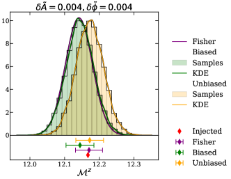
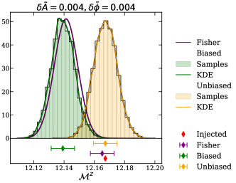
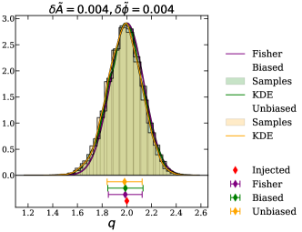
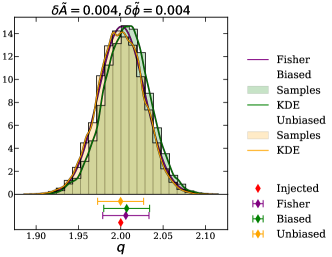
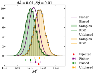
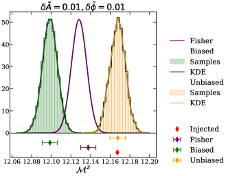
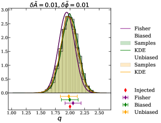
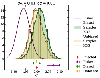
Figure 14: Comparison of full PE results and Fisher matrix estimates. Purple, green and yellow diamonds describe the medians of the corresponding distribution in the panel above (for details on how these are obtained refer to the text). The errorbars represent one standard deviation in each direction.

Appendix B Fisher Matrix Formalism

In section V, we have applied the Fisher matrix formalism to quantify systematic errors, but we have assumed a familiarity with the topic. This section serves as an introduction to the formalism itself, covering important definitions and concepts needed to understand the corresponding discussion in the main text body.

The framework in which Fisher matrix estimates are derived is based on a geometric perspective on PE. Using a metric on the parameter space, the Fisher matrix

$$\Gamma_{\mu\nu}=\langle\partial_{\mu}h,\partial_{\nu}h\rangle\,,$$ (19)

one can derive estimates about various errors in the process. Here, $h$ is some fiducial waveform model and $\partial_{\mu}$ refers to the derivative with respect to the parameter $\Theta^{\mu}$. Eq. (19) is defined in terms of the noise-weighted inner product

$$\langle a,b\rangle=4\Re\int_{f_{\mathrm{low}}}^{f_{\mathrm{high}}}\frac{\tilde{a}(f)\,\tilde{b}^{*}(f)}{S_{n}(f)}\,df\,,$$ (20)

which has already been used in Eq. (3). It is this inner product that several important notions in GW data analysis are based on. Specifically, we will use ‘match’ to refer to the inner product optimized over relative time and phase shifts $t_{0},\phi_{0}$ between $a,b$ and ‘overlap’ to refer to the normalized match, where the result is divided by the product $||a||\cdot||b||$. A complementary notion is the ‘mismatch’, which is defined as $1-\text{match}$.

The Fisher matrix formalism is a very popular tool because it allows to estimate biases in the source parameters $\Theta$, which we will denote as $\Delta\Theta=\Theta_{\mathrm{bf}}-\Theta_{\mathrm{tr}}$. The two parameters $\Theta_{\mathrm{tr}},\Theta_{\mathrm{bf}}$ are to be understood in the following context: say we have data that contains a signal produced by a model $h_{1}$ (and potentially some noise on top of that), and we wish to run PE on this data using another model $h_{2}$; then we call the parameters that $h_{1}$ is evaluated in the ‘true parameters’ $\Theta_{\mathrm{tr}}$ and the parameters obtained from PE ‘best-fitting’ parameters $\Theta_{\mathrm{bf}}$. What the Fisher matrix formalism does for us is that it allows to obtain an estimate of the parameter difference between true and recovered parameters without having to perform a full PE run. This difference will have two contributions: the systematic bias due to $h_{1}\neq h_{2}$ can be estimated as Cutler and Vallisneri (2007)

$$\Delta\Theta^{\mu}_{\mathrm{sys}}=\sum_{\nu}(\Gamma^{-1})^{\mu\nu}\,\langle h_{1}-h_{2},\partial_{\nu}h_{2}\rangle$$ (21)

and the corresponding measurement uncertainty caused by noise (which is also called statistical bias) as Cutler and Vallisneri (2007)

$$\Delta\Theta^{\mu}_{\mathrm{stat}}=\sum_{\nu}(\Gamma^{-1})^{\mu\nu}\langle n,\partial_{\nu}h_{2}\rangle\,.$$ (22)

In reality, where $n$ is not known, it is more common to work with the corresponding standard deviation Cutler and Vallisneri (2007)

$$\sigma_{\Delta\Theta^{\mu}_{\mathrm{stat}}}=\sqrt{(\Gamma^{-1})^{\mu\nu}}\,.$$ (23)

These estimates are very valuable because they can be calculated without having to do an extra PE run. The right hand side of both equations can be evaluated either in the true, injected parameters $\Theta_{\mathrm{tr}}$ or in the best-fitting parameters $\Theta_{\mathrm{bf}}$ that would be the result of a PE run using $h_{2}$ on the signal $h_{1}(\Theta_{\mathrm{tr}})$. To calculate the Fisher matrix in this context, $h_{2}$ must be used.

However, there is also a caveat. The whole approach depends crucially on the validity of the linear signal approximation (LSA)

$$h_{2}(\Theta_{\mathrm{tr}})\simeq h_{2}(\Theta_{\mathrm{bf}})+\partial_{\mu}h_{2}(\Theta_{\mathrm{bf}})(\Theta_{\mathrm{tr}}-\Theta_{\mathrm{bf}})^{\mu}\,.$$ (24)

Besides numerical issues with condition numbers of the Fisher matrix, which are also common problems, this is the major bottleneck of Fisher matrix estimates. If $h_{1}$ and $h_{2}$ exhibit large differences, they might produce maximum-a-posteriori estimates $\Theta_{\mathrm{tr}},\Theta_{\mathrm{bf}}$ for which (24) is not a good approximation. In this case, the accuracy of later applied estimates such as (21), (23) may be compromised.

Recently, the authors of Dhani et al. (2024b) introduced a scheme to improve this issue. The idea, which we only briefly review, is to replace the waveform difference $h_{1}(\Theta_{\mathrm{tr}})-h_{2}(\Theta_{\mathrm{tr}})$ by another difference $h_{1}(\Theta_{\mathrm{tr}})-h_{2}(\overline{\Theta}_{\mathrm{tr}})$ in a procedure called alignment. The new point $\overline{\Theta}_{\mathrm{tr}}$ is defined in such a way that most of its components still coincide with the one of $\Theta_{\mathrm{tr}}$; only the ones that belong to parameters from a set $S$ are changed in order to minimize the normalized inner product

$$\frac{\langle h_{1}(\Theta_{\mathrm{tr}}),h_{2}(\overline{\Theta}_{\mathrm{tr}})\rangle}{\sqrt{\langle h_{1}(\Theta_{\mathrm{tr}}),h_{1}(\Theta_{\mathrm{tr}})\rangle\langle h_{2}(\overline{\Theta}_{\mathrm{tr}}),h_{2}(\overline{\Theta}_{\mathrm{tr}})\rangle}}\,.$$ (25)

In principle, $S$ can contain an arbitrary combination of parameters because there is no restriction as to which parameters can be optimized over in (25). From the motivation, it is natural to select parameters for which conventional differences might occur and as a basic (yet effective) version of $S$, we choose to include relative time and phase shifts $t_{0},\phi_{0}$ (so that (25) coincides with our definition of the ‘overlap’). This also allows a computationally very efficient optimization, exploiting that (20) can be written as an inverse Fourier transform Allen (2005). Of course, the estimate (21) has to be changed accordingly, and the details of how to do this are presented in section III. B. of Ref. Dhani et al. (2024b) (the basic structure remains the same, which is why we do not cover it explicitly here).

B.1 Uncertainty Bands

Here we explain the in detail the purple quantities in Figure 5. The dotted line simply connects points of different SNR for the same values of $\delta\tilde{A},\delta\tilde{\phi}$. In theory, we expect this curve to be a linear function of $\rho$, with known slope. After all, we know that $\Delta\mathcal{M}^{z}$ does not depend on $\rho$ and $\sigma_{\mathcal{M}^{z}}\propto 1/\rho$, so that $\frac{|\Delta\mathcal{M}^{z}|}{\sigma_{\mathcal{M}^{z}}}(\rho)\propto\rho$. Since we know that the SNR between the base signal and high-SNR signal increases by a factor of $5$ (in accordance with the way we adjust $D_{L}$), we expect

$$\begin{split}&\quad\frac{|\Delta\mathcal{M}^{z}|}{\sigma_{\mathcal{M}^{z}}}(\rho_{\mathrm{high-SNR}})=\frac{|\Delta\mathcal{M}^{z}|}{\sigma_{\mathcal{M}^{z}}}(1)\cdot\rho_{\mathrm{high-SNR}}\\ &=\frac{|\Delta\mathcal{M}^{z}|}{\sigma_{\mathcal{M}^{z}}}(1)\cdot 5\cdot\rho_{\mathrm{base}}=5\cdot\frac{|\Delta\mathcal{M}^{z}|}{\sigma_{\mathcal{M}^{z}}}(\rho_{\mathrm{base}})\,.\end{split}$$ (26)

However, due to sampling uncertainties, this is not strictly true. To visualize this effect, we draw the shaded, purple uncertainty bands. We quantify the uncertainty in slope using the following, simple model: from table 2 we can calculate

$$|\Delta\mathcal{M}^{z}(\rho_{\mathrm{high-SNR}})-\Delta\mathcal{M}^{z}(\rho_{\mathrm{base}})|=0.005$$ (27)

(coincidentally, for both configurations that we discuss). This number is on par with differences between injected values and unbiased recovery for the non-high-SNR injections, so that an origin other than sampling uncertainties is unlikely. We then calculate the linear fits through all combinations of the two points $\frac{|\Delta\mathcal{M}^{z}\pm 0.005|}{\sigma_{\mathcal{M}^{z}}}(\rho_{\mathrm{base}}),\frac{|\Delta\mathcal{M}^{z}\pm 0.005|}{\sigma_{\mathcal{M}^{z}}}(\rho_{\mathrm{high-SNR}})$. The minimum (maximum) of all those fits determines the lower (upper) uncertainty band in Figure 5.

The advantage of showing these bands is that they allow to assess how well the Fisher estimates reproduce the PE results. If they only deviate on a level that is consistent with deviations produced by sampling uncertainties, then we can claim good agreement. Evidently, the rel-phase model can be reproduced well for the ‘LSA-case’ as the blue line in Figure 5 (a) lies within the uncertainty band. For the ‘non-LSA case’, on the other hand, the estimate performs worse (which is consistent with the findings from table 2). Looking at the abs-phase configurations, we see that the one with $\delta\tilde{A}=0.01,\delta\tilde{\phi}\sim\mathcal{N}(0.2,0.1)$ has noticeably larger uncertainty bands compared to the other ones. This can be explained by the fact that the systematic biases are small for this configuration, so that sampling uncertainties show up very prominently. This leads to large variation in slopes obtained by procedure outlined above, leading to the large band observed there. For this, it is usually the non-high-SNR case that is to blame. For the high-SNR runs the PE runs can locate the posterior peak with much more accuracy (compared to non-high-SNR), since the width is much smaller, making parameters with some deviation from the peak strongly disfavored by the high-SNR likelihood, while they might only be mildly disfavored by the non-high-SNR likelihood.

B.2 Another Perspective On The Fisher Matrix Results

In the main body, we have used table 2 to collectively represent the results that compare full PE and Fisher matrix estimates. There we have focused on the numbers for systematic bias $\Delta\Theta_{\mathrm{sys}}$ and standard deviation $\sigma_{\Delta\Theta_{\mathrm{stat}}}$. However, we have not considered the following: under the LSA, the likelihood is a Gaussian around the corresponding maximum a posteriori estimate $\theta_{\mathrm{max}}$ with standard deviation $\sigma_{\Theta^{\mu}}=\sigma_{\Delta\Theta_{\mathrm{stat}}}$. Consequently, a visual test of the Fisher estimates can be done using these two numbers: given $\Theta_{\mathrm{max,biased}}$ from the biased PE run (where we recover an injection with waveform error using a model that does not account for waveform errors), we can estimate what the unbiased distribution should look like via

$$\mathcal{N}(\Theta_{\mathrm{max,unbiased}},\sigma_{\Theta^{\mu}})=\mathcal{N}(\Theta_{\mathrm{max,biased}}+\Delta\Theta,\sigma_{\Delta\Theta_{\mathrm{stat}}})\,.$$ (28)

Fig. 14 shows how these estimates compare to the unbiased distributions obtained from actually running PE (we expect their median to reproduce the injected value). For the purple distributions that are computed according to (28), it is reasonable to assume that these already represent the posteriors and not just the likelihood, so we do not account for priors separately. This assumption is justified since $\Theta_{\mathrm{max,biased}}$ already contains prior information, which means that $\Theta_{\mathrm{max,unbiased}}$ does, too (strictly speaking, that means we assume the priors to be constant over the range given by $\Delta\Theta_{\mathrm{sys}}$).

Appendix C Additional details of simulations and PE results

In the examples we considered in section VI, we find that it is primarily the $\delta\phi$ parameter (for both the parametrizations) that is constrained by the data. We obtain the prior distribution only for the $\delta\tilde{A}$. It can be understood because, in our simulations, we introduce $1-2\%$ relative errors in amplitude. It seems too low for the simulations to pick up variation of that order in the amplitude parameter. Moreover, a constant shift of $\delta\tilde{A}$ is expected to be absorbed in distance posteriors. For the 2G PE analysis, we can use WF-Error parametrizations (8), and (9) which uses only $\delta\tilde{\phi}$ parameter. We choose to keep the $\delta\tilde{A}$ in our parametrizations to account for most general cases of deviation.

References

- Aasi et al. (2015) J. Aasi et al. (LIGO Scientific), Class. Quant. Grav. 32, 074001 (2015), arXiv:1411.4547 [gr-qc] .
- Buikema et al. (2020) A. Buikema et al. (aLIGO), Phys. Rev. D 102, 062003 (2020), arXiv:2008.01301 [astro-ph.IM] .
- Abbott et al. (2016a) B. P. Abbott et al. (KAGRA, LIGO Scientific, Virgo), Living Rev. Rel. 19, 1 (2016a), arXiv:1304.0670 [gr-qc] .
- Acernese et al. (2015) F. Acernese et al. (VIRGO), Class. Quant. Grav. 32, 024001 (2015), arXiv:1408.3978 [gr-qc] .
- Acernese et al. (2019) F. Acernese et al. (Virgo), Phys. Rev. Lett. 123, 231108 (2019).
- The LIGO Scientific Collaboration et al. (2021a) The LIGO Scientific Collaboration, The Virgo Collaboration, The KAGRA Collaboration, et al., “GWTC-3: Compact Binary Coalescences Observed by LIGO and Virgo During the Second Part of the Third Observing Run,” (2021a).
- Nitz et al. (2023) A. H. Nitz, S. Kumar, Y.-F. Wang, S. Kastha, S. Wu, M. Schäfer, R. Dhurkunde, and C. D. Capano, Astrophys. J. 946, 59 (2023), arXiv:2112.06878 [astro-ph.HE] .
- Wadekar et al. (2023) D. Wadekar, J. Roulet, T. Venumadhav, A. K. Mehta, B. Zackay, J. Mushkin, S. Olsen, and M. Zaldarriaga, (2023), arXiv:2312.06631 [gr-qc] .
- Abbott et al. (2021a) R. Abbott et al. (LIGO Scientific, VIRGO, KAGRA), (2021a), arXiv:2112.06861 [gr-qc] .
- Abbott et al. (2023a) R. Abbott et al. (KAGRA, VIRGO, LIGO Scientific), Phys. Rev. X 13, 011048 (2023a), arXiv:2111.03634 [astro-ph.HE] .
- Abbott et al. (2021b) R. Abbott et al. (LIGO Scientific, VIRGO, KAGRA), (2021b), arXiv:2111.03604 [astro-ph.CO] .
- Abbott et al. (2018) B. P. Abbott et al. (LIGO Scientific, Virgo), Phys. Rev. Lett. 121, 161101 (2018), arXiv:1805.11581 [gr-qc] .
- Abbott et al. (2019a) B. P. Abbott et al. (LIGO Scientific, Virgo), Phys. Rev. X 9, 011001 (2019a), arXiv:1805.11579 [gr-qc] .
- Capano et al. (2020) C. D. Capano, I. Tews, S. M. Brown, B. Margalit, S. De, S. Kumar, D. A. Brown, B. Krishnan, and S. Reddy, Nature Astron. 4, 625 (2020), arXiv:1908.10352 [astro-ph.HE] .
- Blanchet (2014) L. Blanchet, Living Rev. Rel. 17, 2 (2014), arXiv:1310.1528 [gr-qc] .
- Campanelli et al. (2006) M. Campanelli, C. O. Lousto, P. Marronetti, and Y. Zlochower, Phys. Rev. Lett. 96, 111101 (2006), arXiv:gr-qc/0511048 .
- Pretorius (2005) F. Pretorius, Phys. Rev. Lett. 95, 121101 (2005), arXiv:gr-qc/0507014 .
- Baker et al. (2006) J. G. Baker, J. Centrella, D.-I. Choi, M. Koppitz, and J. van Meter, Phys. Rev. Lett. 96, 111102 (2006), arXiv:gr-qc/0511103 .
- Abbott et al. (2016b) B. P. Abbott et al., Phys. Rev. D 93, 112004 (2016b), [Addendum: Phys.Rev.D 97, 059901 (2018)], arXiv:1604.00439 [astro-ph.IM] .
- Saleem et al. (2022) M. Saleem et al., Class. Quant. Grav. 39, 025004 (2022), arXiv:2105.01716 [gr-qc] .
- Punturo et al. (2010) M. Punturo et al., Class. Quant. Grav. 27, 084007 (2010).
- Hild et al. (2011) S. Hild et al., Class. Quant. Grav. 28, 094013 (2011), arXiv:1012.0908 [gr-qc] .
- Evans et al. (2021) M. Evans et al., (2021), arXiv:2109.09882 [astro-ph.IM] .
- Srivastava et al. (2022) V. Srivastava, D. Davis, K. Kuns, P. Landry, S. Ballmer, M. Evans, E. D. Hall, J. Read, and B. S. Sathyaprakash, Astrophys. J. 931, 22 (2022), arXiv:2201.10668 [gr-qc] .
- Evans et al. (2023) M. Evans et al., (2023), arXiv:2306.13745 [astro-ph.IM] .
- Lindblom et al. (2008) L. Lindblom, B. J. Owen, and D. A. Brown, Phys. Rev. D 78, 124020 (2008), arXiv:0809.3844 [gr-qc] .
- Pürrer and Haster (2020) M. Pürrer and C.-J. Haster, Phys. Rev. Res. 2, 023151 (2020), arXiv:1912.10055 [gr-qc] .
- Dhani et al. (2024a) A. Dhani, S. Völkel, A. Buonanno, H. Estelles, J. Gair, H. P. Pfeiffer, L. Pompili, and A. Toubiana, (2024a), arXiv:2404.05811 [gr-qc] .
- Kumar et al. (2022) S. Kumar, A. H. Nitz, and X. J. Forteza, (2022), arXiv:2202.12762 [astro-ph.IM] .
- Gupta et al. (2024) A. Gupta et al., (2024), 10.21468/SciPostPhysCommRep.5, arXiv:2405.02197 [gr-qc] .
- Read (2023) J. S. Read, Class. Quant. Grav. 40, 135002 (2023), arXiv:2301.06630 [gr-qc] .
- Abbott et al. (2023b) R. Abbott et al. (KAGRA, VIRGO, LIGO Scientific), Phys. Rev. X 13, 041039 (2023b), arXiv:2111.03606 [gr-qc] .
- Ashton and Khan (2020) G. Ashton and S. Khan, Phys. Rev. D 101, 064037 (2020), arXiv:1910.09138 [gr-qc] .
- Jan et al. (2020) A. Z. Jan, A. B. Yelikar, J. Lange, and R. O’Shaughnessy, Phys. Rev. D 102, 124069 (2020), arXiv:2011.03571 [gr-qc] .
- Ashton and Dietrich (2022) G. Ashton and T. Dietrich, Nature Astron. 6, 961 (2022), arXiv:2111.09214 [gr-qc] .
- Hoy (2022) C. Hoy, Phys. Rev. D 106, 083003 (2022), arXiv:2208.00106 [gr-qc] .
- Puecher et al. (2024) A. Puecher, A. Samajdar, G. Ashton, C. Van Den Broeck, and T. Dietrich, Phys. Rev. D 109, 023019 (2024), arXiv:2310.03555 [gr-qc] .
- Samajdar and Dietrich (2018) A. Samajdar and T. Dietrich, Phys. Rev. D 98, 124030 (2018).
- Samajdar and Dietrich (2019) A. Samajdar and T. Dietrich, Phys. Rev. D 100, 024046 (2019).
- Hoy et al. (2024) C. Hoy, S. Akcay, J. Mac Uilliam, and J. E. Thompson, (2024), arXiv:2409.19404 [gr-qc] .
- Moore and Gair (2014) C. J. Moore and J. R. Gair, Phys. Rev. Lett. 113, 251101 (2014).
- Pompili et al. (2024) L. Pompili, A. Buonanno, and M. Pürrer, (2024), arXiv:2410.16859 [gr-qc] .
- Bachhar et al. (2024) R. Bachhar, M. Pürrer, and S. R. Green, (2024), arXiv:2410.17168 [gr-qc] .
- Khan (2024) S. Khan, Phys. Rev. D 109, 104045 (2024).
- Owen et al. (2023) C. B. Owen, C.-J. Haster, S. Perkins, N. J. Cornish, and N. Yunes, Phys. Rev. D 108, 044018 (2023), arXiv:2301.11941 [gr-qc] .
- Detweiler and Brown (1997) S. L. Detweiler and L. H. Brown, Jr., Phys. Rev. D 56, 826 (1997), arXiv:gr-qc/9609010 .
- Bern et al. (2019) Z. Bern, C. Cheung, R. Roiban, C.-H. Shen, M. P. Solon, and M. Zeng, Phys. Rev. Lett. 122, 201603 (2019), arXiv:1901.04424 [hep-th] .
- Vishveshwara (1970) C. V. Vishveshwara, Nature 227, 936 (1970).
- Chandrasekhar and Detweiler (1975) S. Chandrasekhar and S. L. Detweiler, Proc. Roy. Soc. Lond. A 344, 441 (1975).
- Ohme (2012) F. Ohme, Class. Quant. Grav. 29, 124002 (2012), arXiv:1111.3737 [gr-qc] .
- Ajith et al. (2008) P. Ajith et al., Phys. Rev. D 77, 104017 (2008), [Erratum: Phys.Rev.D 79, 129901 (2009)], arXiv:0710.2335 [gr-qc] .
- Ajith et al. (2011) P. Ajith et al., Phys. Rev. Lett. 106, 241101 (2011), arXiv:0909.2867 [gr-qc] .
- Santamaria et al. (2010) L. Santamaria et al., Phys. Rev. D 82, 064016 (2010), arXiv:1005.3306 [gr-qc] .
- Khan et al. (2016) S. Khan, S. Husa, M. Hannam, F. Ohme, M. Pürrer, X. Jiménez Forteza, and A. Bohé, Phys. Rev. D 93, 044007 (2016), arXiv:1508.07253 [gr-qc] .
- Khan et al. (2019) S. Khan, K. Chatziioannou, M. Hannam, and F. Ohme, Phys. Rev. D 100, 024059 (2019), arXiv:1809.10113 [gr-qc] .
- Khan et al. (2020) S. Khan, F. Ohme, K. Chatziioannou, and M. Hannam, Phys. Rev. D 101, 024056 (2020), arXiv:1911.06050 [gr-qc] .
- Husa et al. (2016) S. Husa, S. Khan, M. Hannam, M. Pürrer, F. Ohme, X. Jiménez Forteza, and A. Bohé, Phys. Rev. D 93, 044006 (2016), arXiv:1508.07250 [gr-qc] .
- London et al. (2018) L. London, S. Khan, E. Fauchon-Jones, C. García, M. Hannam, S. Husa, X. Jiménez-Forteza, C. Kalaghatgi, F. Ohme, and F. Pannarale, Phys. Rev. Lett. 120, 161102 (2018), arXiv:1708.00404 [gr-qc] .
- Hannam et al. (2014) M. Hannam, P. Schmidt, A. Bohé, L. Haegel, S. Husa, F. Ohme, G. Pratten, and M. Pürrer, Phys. Rev. Lett. 113, 151101 (2014), arXiv:1308.3271 [gr-qc] .
- García-Quirós et al. (2020) C. García-Quirós, M. Colleoni, S. Husa, H. Estellés, G. Pratten, A. Ramos-Buades, M. Mateu-Lucena, and R. Jaume, Phys. Rev. D 102, 064002 (2020), arXiv:2001.10914 [gr-qc] .
- Pratten et al. (2021) G. Pratten et al., Phys. Rev. D 103, 104056 (2021), arXiv:2004.06503 [gr-qc] .
- Pratten et al. (2020) G. Pratten, S. Husa, C. Garcia-Quiros, M. Colleoni, A. Ramos-Buades, H. Estelles, and R. Jaume, Phys. Rev. D 102, 064001 (2020), arXiv:2001.11412 [gr-qc] .
- Estellés et al. (2021) H. Estellés, A. Ramos-Buades, S. Husa, C. García-Quirós, M. Colleoni, L. Haegel, and R. Jaume, Phys. Rev. D 103, 124060 (2021), arXiv:2004.08302 [gr-qc] .
- Estellés et al. (2022) H. Estellés, M. Colleoni, C. García-Quirós, S. Husa, D. Keitel, M. Mateu-Lucena, M. d. L. Planas, and A. Ramos-Buades, Phys. Rev. D 105, 084040 (2022), arXiv:2105.05872 [gr-qc] .
- Ghosh et al. (2024) S. Ghosh, P. Kolitsidou, and M. Hannam, Phys. Rev. D 109, 024061 (2024), arXiv:2310.16980 [gr-qc] .
- Thompson et al. (2024) J. E. Thompson, E. Hamilton, L. London, S. Ghosh, P. Kolitsidou, C. Hoy, and M. Hannam, Phys. Rev. D 109, 063012 (2024), arXiv:2312.10025 [gr-qc] .
- Buonanno and Damour (1999) A. Buonanno and T. Damour, Phys. Rev. D 59, 084006 (1999), arXiv:gr-qc/9811091 .
- Pan et al. (2011) Y. Pan, A. Buonanno, M. Boyle, L. T. Buchman, L. E. Kidder, H. P. Pfeiffer, and M. A. Scheel, Phys. Rev. D 84, 124052 (2011), arXiv:1106.1021 [gr-qc] .
- Pan et al. (2014) Y. Pan, A. Buonanno, A. Taracchini, L. E. Kidder, A. H. Mroué, H. P. Pfeiffer, M. A. Scheel, and B. Szilágyi, Phys. Rev. D 89, 084006 (2014), arXiv:1307.6232 [gr-qc] .
- Taracchini et al. (2014) A. Taracchini et al., Phys. Rev. D 89, 061502 (2014), arXiv:1311.2544 [gr-qc] .
- Bohé et al. (2017) A. Bohé et al., Phys. Rev. D 95, 044028 (2017), arXiv:1611.03703 [gr-qc] .
- Cotesta et al. (2018) R. Cotesta, A. Buonanno, A. Bohé, A. Taracchini, I. Hinder, and S. Ossokine, Phys. Rev. D 98, 084028 (2018), arXiv:1803.10701 [gr-qc] .
- Ossokine et al. (2020) S. Ossokine et al., Phys. Rev. D 102, 044055 (2020), arXiv:2004.09442 [gr-qc] .
- Pompili et al. (2023) L. Pompili et al., Phys. Rev. D 108, 124035 (2023), arXiv:2303.18039 [gr-qc] .
- Gamboa et al. (2024) A. Gamboa et al., (2024), arXiv:2412.12823 [gr-qc] .
- Damour et al. (2013) T. Damour, A. Nagar, and S. Bernuzzi, Phys. Rev. D 87, 084035 (2013), arXiv:1212.4357 [gr-qc] .
- Gamba et al. (2021) R. Gamba, S. Bernuzzi, and A. Nagar, Phys. Rev. D 104, 084058 (2021), arXiv:2012.00027 [gr-qc] .
- Nagar et al. (2024) A. Nagar, S. Bernuzzi, D. Chiaramello, V. Fantini, R. Gamba, M. Panzeri, and P. Rettegno, (2024), arXiv:2407.04762 [gr-qc] .
- Field et al. (2014) S. E. Field, C. R. Galley, J. S. Hesthaven, J. Kaye, and M. Tiglio, Phys. Rev. X 4, 031006 (2014), arXiv:1308.3565 [gr-qc] .
- Blackman et al. (2017a) J. Blackman, S. E. Field, M. A. Scheel, C. R. Galley, D. A. Hemberger, P. Schmidt, and R. Smith, Phys. Rev. D 95, 104023 (2017a), arXiv:1701.00550 [gr-qc] .
- Blackman et al. (2017b) J. Blackman, S. E. Field, M. A. Scheel, C. R. Galley, C. D. Ott, M. Boyle, L. E. Kidder, H. P. Pfeiffer, and B. Szilágyi, Phys. Rev. D 96, 024058 (2017b), arXiv:1705.07089 [gr-qc] .
- Varma et al. (2019a) V. Varma, S. E. Field, M. A. Scheel, J. Blackman, L. E. Kidder, and H. P. Pfeiffer, Phys. Rev. D 99, 064045 (2019a), arXiv:1812.07865 [gr-qc] .
- Varma et al. (2019b) V. Varma, S. E. Field, M. A. Scheel, J. Blackman, D. Gerosa, L. C. Stein, L. E. Kidder, and H. P. Pfeiffer, Phys. Rev. Research. 1, 033015 (2019b), arXiv:1905.09300 [gr-qc] .
- Abbott et al. (2020a) B. P. Abbott et al. (LIGO Scientific, Virgo), Class. Quant. Grav. 37, 055002 (2020a), arXiv:1908.11170 [gr-qc] .
- Prix (2007) R. Prix, Class. Quant. Grav. 24, S481 (2007), arXiv:0707.0428 [gr-qc] .
- Usman et al. (2016) S. A. Usman et al., Class. Quant. Grav. 33, 215004 (2016), arXiv:1508.02357 [gr-qc] .
- Allen (2021) B. Allen, Phys. Rev. D 104, 042005 (2021), arXiv:2102.11254 [astro-ph.IM] .
- Veitch et al. (2015) J. Veitch et al., Phys. Rev. D 91, 042003 (2015), arXiv:1409.7215 [gr-qc] .
- Biwer et al. (2019) C. M. Biwer, C. D. Capano, S. De, M. Cabero, D. A. Brown, A. H. Nitz, and V. Raymond, Publ. Astron. Soc. Pac. 131, 024503 (2019), arXiv:1807.10312 [astro-ph.IM] .
- Mozzon et al. (2020) S. Mozzon, L. K. Nuttall, A. Lundgren, T. Dent, S. Kumar, and A. H. Nitz, Classical and Quantum Gravity 37, 215014 (2020).
- Edy et al. (2021) O. Edy, A. Lundgren, and L. K. Nuttall, Physical Review D 103 (2021), 10.1103/physrevd.103.124061.
- Edelman et al. (2021) B. Edelman et al., Phys. Rev. D 103, 042004 (2021), arXiv:2008.06436 [gr-qc] .
- Abbott et al. (2020b) R. Abbott et al. (LIGO Scientific, Virgo), Phys. Rev. D 102, 043015 (2020b), arXiv:2004.08342 [astro-ph.HE] .
- LIGO Scientific Collaboration (2018) LIGO Scientific Collaboration, “LIGO Algorithm Library - LALSuite,” free software (GPL) (2018).
- Cahillane et al. (2017) C. Cahillane, J. Betzwieser, D. A. Brown, E. Goetz, E. D. Hall, K. Izumi, S. Kandhasamy, S. Karki, J. S. Kissel, G. Mendell, R. L. Savage, D. Tuyenbayev, A. Urban, A. Viets, M. Wade, and A. J. Weinstein, Phys. Rev. D 96, 102001 (2017), arXiv:1708.03023 [astro-ph.IM] .
- Sun et al. (2020) L. Sun et al., Class. Quant. Grav. 37, 225008 (2020), arXiv:2005.02531 [astro-ph.IM] .
- Sun et al. (2021) L. Sun et al., (2021), arXiv:2107.00129 [astro-ph.IM] .
- Acernese et al. (2022) F. Acernese et al. (VIRGO), Class. Quant. Grav. 39, 045006 (2022), arXiv:2107.03294 [gr-qc] .
- Acernese et al. (2018) F. Acernese et al. (Virgo), Class. Quant. Grav. 35, 205004 (2018), arXiv:1807.03275 [gr-qc] .
- (100) “LIGO-T2100313-v3: LIGO and Virgo Calibration Uncertainty (O1, O2 and O3) — dcc.ligo.org,” https://dcc.ligo.org/T2100313/public, [Accessed 10-02-2025].
- Farr et al. (2015) W. M. Farr, B. Farr, and T. Littenberg, Modelling Calibration Errors In CBC Waveforms, Tech. Rep. LIGO-T1400682 (LIGO Project, 2015).
- Cahillane et al. (2017) C. Cahillane et al. (LIGO Scientific), Phys. Rev. D 96, 102001 (2017), arXiv:1708.03023 [astro-ph.IM] .
- Dhani et al. (2024b) A. Dhani, S. Völkel, A. Buonanno, H. Estelles, J. Gair, H. P. Pfeiffer, L. Pompili, and A. Toubiana, “Systematic biases in estimating the properties of black holes due to inaccurate gravitational-wave models,” (2024b), arXiv:2404.05811 [gr-qc] .
- Dupletsa et al. (2024) U. Dupletsa, J. Harms, K. K. Y. Ng, J. Tissino, F. Santoliquido, and A. Cozzumbo, “Validating prior-informed fisher-matrix analyses against gwtc data,” (2024), arXiv:2404.16103 [gr-qc] .
- Abbott et al. (2019b) B. P. Abbott et al., Physical Review X 9 (2019b), 10.1103/physrevx.9.031040.
- Abbott et al. (2021c) R. Abbott et al., Physical Review X 11 (2021c), 10.1103/physrevx.11.021053.
- The LIGO Scientific Collaboration et al. (2021b) The LIGO Scientific Collaboration, The Virgo Collaboration, et al., “GWTC-2.1: Deep Extended Catalog of Compact Binary Coalescences Observed by LIGO and Virgo During the First Half of the Third Observing Run,” (2021b).
- Vallisneri (2008) M. Vallisneri, Physical Review D 77 (2008), 10.1103/physrevd.77.042001.
- Speagle (2020) J. S. Speagle, Monthly Notices of the Royal Astronomical Society 493, 3132 (2020), https://academic.oup.com/mnras/article-pdf/493/3/3132/32890730/staa278.pdf .
- Kumar et al. (2025) S. Kumar, M. Melching, and F. Ohme, “PyCBC plugin for waveform errors,” https://github.com/gwastro/pycbc_wferrors_plugin (2025).
- Paul and Mishra (2023) K. Paul and C. K. Mishra, Phys. Rev. D 108, 024023 (2023), arXiv:2211.04155 [gr-qc] .
- Henry and Khalil (2023) Q. Henry and M. Khalil, Phys. Rev. D 108, 104016 (2023), arXiv:2308.13606 [gr-qc] .
- Ramos-Buades et al. (2022) A. Ramos-Buades, A. Buonanno, M. Khalil, and S. Ossokine, Phys. Rev. D 105, 044035 (2022), arXiv:2112.06952 [gr-qc] .
- Paul et al. (2024) K. Paul, A. Maurya, Q. Henry, K. Sharma, P. Satheesh, Divyajyoti, P. Kumar, and C. K. Mishra, (2024), arXiv:2409.13866 [gr-qc] .
- Virtanen et al. (2020) P. Virtanen, R. Gommers, T. E. Oliphant, M. Haberland, T. Reddy, D. Cournapeau, E. Burovski, P. Peterson, W. Weckesser, J. Bright, S. J. van der Walt, M. Brett, J. Wilson, K. J. Millman, N. Mayorov, A. R. J. Nelson, E. Jones, R. Kern, E. Larson, C. J. Carey, İ. Polat, Y. Feng, E. W. Moore, J. VanderPlas, D. Laxalde, J. Perktold, R. Cimrman, I. Henriksen, E. A. Quintero, C. R. Harris, A. M. Archibald, A. H. Ribeiro, F. Pedregosa, P. van Mulbregt, and SciPy 1.0 Contributors, Nature Methods 17, 261 (2020).
- Cutler and Vallisneri (2007) C. Cutler and M. Vallisneri, Physical Review D 76 (2007), 10.1103/physrevd.76.104018.
- Balasubramanian et al. (1996) R. Balasubramanian, B. S. Sathyaprakash, and S. V. Dhurandhar, Phys. Rev. D 53, 3033 (1996).
- Allen (2005) B. Allen, Physical Review D 71 (2005), 10.1103/physrevd.71.062001.