Advances in multiparameter quantum sensing and metrology

Résumé

Recent years have witnessed a growing interest in understating the limitations imposed by quantum noise in precision measurements and devising techniques to reduce it. The attention is currently turning to the simultaneously estimation of several parameters of interest, driven by its promising potential across a wide range of sensing applications as well as fueled by experimental progress in various optical and atomic platforms. Here, we provide a comprehensive overview of key research directions in multiparameter quantum sensing and metrology, highlighting both opportunities and challenges. We introduce the basic framework, discuss ultimate sensitivity bounds, optimal measurement strategies, and the role of quantum incompatibility, showing important differences with respect to single-parameter estimation. Additionally, we discuss emerging experimental implementations in distributed quantum sensing, including cutting-edge optimization techniques. This review aims to bridge the gap between theory and experiments, paving the way for the next-generation of quantum sensors and their integration with other quantum technologies.

5 mars 2025

Introduction. Multiparameter sensing focuses on the simultaneous estimation of several parameters. This task has a broad range of applications, where the achievable precision is – or will soon be – fundamentally limited by the intrinsic quantum noise. For example, quantum networks of atomic clocks ZollerPRL2024 ; KomarNATPHYS2014 enhance precision measurements over large distances, enabling unprecedented synchronization and stability. Optical imaging AlbarelliPLA2020 and magnetic field mapping DegenRMP2017 impact medicine and biology BowenPR2016 ; AslamNRP2023 , improving monitoring and diagnostics. Vectorial force sensing enables high-precision inertial navigation GracePRAPP2020 . Learning quantum systems GebhartNRP2023 , designing quantum gates and algorithms BhartiRMP2022 and communication networks WehnerSCIENCE2018 can involve the estimation and the optimization of multiple parameters. Furthermore, the real-time simultaneous estimation of phase and phase diffusion helps reduce systematic errors VidrighinNATCOMM2014 .

The aim of this review is to explore possibilities and challenges in multiparameter quantum sensing and metrology. Recent theoretical and experimental studies have highlighted how quantum resources – such as entanglement and squeezing – can reduce the impact of quantum noise and thus enhance the performance of multiparameter estimation beyond what is possible using independent sensors and particles. However, the intrinsic incompatibility inherent in quantum mechanics, coupled with the curse of dimensionality, renders the identification of optimal protocols and sensitivity bounds far richer and more challenging than in the single-parameter scenario. For these reasons, advanced numerical techniques, including machine learning and variational approaches, may boost accuracy and enable real-time data processing and adaptive decision-making. Finally, sensors exploiting quantum resources are generally highly sensitive to external noise and decoherence, which can significantly impair their performance. Implementing noise mitigation strategies, fault tolerance, and quantum error correction is therefore essential for maintaining high precision in applications.

General framework. A generic quantum probe state $\rho$ undergoes a quantum channel transformation that simultaneously encodes the values of $d$ parameters $\bm{\theta}=\{\theta_{1},...,\theta_{d}\}^{\top}$ that we want to estimate. Information about the unknown $\bm{\theta}$ is extracted from measurements performed on the transformed state $\rho_{\bm{\theta}}$. The detection process is generally described by a positive operator-valued measure (POVM), $\bm{E}=\{E_{1},E_{2}...\}^{\top}$, namely a set of non-negative operators ($E_{k}\geq 0$) satisfying the completeness relation $\sum_{k}E_{k}=\mathbbm{1}$. Each measurement outcome, labeled by $k$, occurs with probability $P(k|\bm{\theta})={\rm Tr}[\rho_{\bm{\theta}}E_{k}]$ according to the Born rule. By repeating the measurement $m$ times, a sequence of independent outcomes $\bm{k}=\{k_{1},...,k_{m}\}^{\top}$ is collected. Finally, an estimator function, $\Theta_{j}(\bm{k})$ provides an estimate for each parameter $\theta_{j}$. In the following, we assume locally-unbiased estimators, namely satisfying $\bar{\bm{\Theta}}=\sum_{\bm{k}}P(\bm{k}|\bm{\theta})\bm{\Theta}(\bm{k})=\bm{\theta}$ and $\bm{\nabla}_{\bm{\theta}}\bar{\bm{\Theta}}=\mathbbm{1}_{d}$, where $\bm{\Theta}(\bm{k})=\{\Theta_{1}(\bm{k}),...,\Theta_{d}(\bm{k})\}^{\top}$ and $P(k|\bm{\theta})=\prod_{j=1}^{m}P(k_{j}|\bm{\theta})$ is the probability to observe the measurement sequence. The aim of multiparameter quantum metrology is to identify the best combinations of probe states, POVMs, and estimators that enhance accuracy and precision, potentially incorporating optimal control protocols, ancillary subsystems, and/or joint measurements performed on multiple copies of $\rho_{\bm{\theta}}$.

Figure 1: Multiparameter estimation in the quantum setting. Multiparameter estimation proceeds through a series of sequential steps: state preparation, simultaneous encoding of the several parameters described by a quantum channel, detection, and estimation. In the simplest scenario (a), the protocol involves a single quantum probe state $\rho$: this is commonly referred to as a single-copy measurement. In a more general scenario (b), joint measurements are performed on multiple ($n>1$) independent copies of the probe state, namely on $\rho_{\bm{\theta}}^{\otimes n}$. In contrast to the single-parameter framework GiovannettiNATPHOT2011 ; PezzeRMP2018 , joint measurements are typically optimal and necessary to saturate the ultimate quantum sensitivity bounds.

Quantum bounds. The estimation uncertainty is quantified by the $d\times d$ covariance matrix of estimators,

$$\bm{C}(\rho_{\bm{\theta}},\bm{E},\bm{\Theta})=\sum_{\bm{k}}P(\bm{k}|\bm{\theta})[\bm{\theta}-\bm{\bm{\Theta}}(\bm{k})][\bm{\theta}-\bm{\bm{\Theta}}(\bm{k})]^{\top}.$$ (1)

The diagonal element $\bm{C}_{jj}$ is the variance of $\Theta_{j}$, while the off-diagonal term $\bm{C}_{ij}$ provides statistical correlations between $\Theta_{i}$ and $\Theta_{j}$. Equation (1) fulfills the chain of matrix inequalities HelstromBOOK1976

$$\bm{C}(\rho_{\bm{\theta}},\bm{E},\bm{\Theta})\geq\frac{\bm{F}^{-1}(\rho_{\bm{\theta}},\bm{E})}{m}\geq\frac{\bm{F}_{Q}^{-1}(\rho_{\bm{\theta}})}{m}.$$ (2)

The first inequality is the multiparameter Cramér-Rao bound (CRB). It is obtained by minimizing $\bm{C}$ over all possible unbiased estimators, where $\bm{F}(\rho_{\bm{\theta}},\bm{E})$ is the Fisher information matrix (FIM), see Box. Advances in multiparameter quantum sensing and metrology. The inequality can be saturated by optimal locally-unbiased estimators, such as the maximum likelihood in the limit $m\gg 1$ KayBOOK1993 . The second inequality is the multiparameter quantum Cramér-Rao bound (QCRB) HelstromBOOK1976 , where $\bm{F}_{Q}(\rho_{\bm{\theta}})$ is the quantum Fisher information matrix (QFIM), see Box. Advances in multiparameter quantum sensing and metrology. The meaning of Eq. (2) is that the variance of any linear function of the parameters, $\bm{\nu}^{\top}\bm{\theta}=\sum_{j=1}^{d}\nu_{j}\theta_{j}$, fulfills

$$\Delta^{2}(\bm{\nu}^{\top}\bm{\theta})=\bm{\nu}^{\top}\bm{C}\bm{\nu}\geq\frac{\bm{\nu}^{\top}\bm{F}^{-1}\bm{\nu}}{m}\geq\frac{\bm{\nu}^{\top}\bm{F}_{Q}^{-1}\bm{\nu}}{m},$$ (3)

where the real vector $\bm{\nu}=\{\nu_{1},...,\nu_{d}\}^{\top}$ specifies the combination of interest. The other combinations orthogonal to $\bm{\nu}$ play the role of nuisance parameters SuzukiJPA2020 and generally affect $\Delta^{2}(\bm{\nu}^{\top}\bm{\theta})$. Similarly to the single-parameter case ($d=1$) BraunsteinPRL1994 , it can be proved that there is always an optimal $\bm{\nu}$-dependent POVM that saturates the last inequality in Eq. (3) SuzukiJPA2020 . Moreover, the eigenvector of the FIM (QFIM) corresponding to its largest eigenvalue determines the combination of the parameters that attains the lowest uncertainty for a given (optimal) POVM.

In the multiparameter scenario, one may be interested in estimating several (not necessarily orthogonal) linear combinations of the parameters, $\bm{\nu}^{\top}_{j}\bm{\theta}$, with $j=1,2,...$. Each combination is weighted by a positive factor $w_{j}>0$, reflecting the desired trade-off among the variances $\Delta^{2}(\bm{\nu}_{j}^{\top}\bm{\theta})$. The figure of merit generalizes to $\sum_{j}w_{j}\Delta^{2}(\bm{\nu}_{j}^{\top}\bm{\theta})={\rm Tr}[\bm{C}\bm{W}]$, where the $d\times d$ weight matrix $\bm{W}=\sum_{j}w_{j}\bm{\nu}_{j}\bm{\nu}_{j}^{T}$ is real, symmetric and positive definite. In this case, finding the ultimate sensitivity bound – referred to as the most informative bound (MIB) – is highly nontrivial. The MIB is defined as $\mathscr{B}_{\rm MI}(\rho_{\bm{\theta}},\bm{W})=\min_{\bm{E}}\mathscr{B}_{\rm CR}(\rho_{\bm{\theta}},\bm{E},\bm{W})$, where $\mathscr{B}_{\rm CR}(\rho_{\bm{\theta}},\bm{E},\bm{W})={\rm Tr}[\bm{W}\bm{F}^{-1}]$. It corresponds to the minimum of $m{\rm Tr}[\bm{C}\bm{W}]$ over all possible locally-unbiased estimators and POVMs, and is attainable for $m\gg 1$, at least. Although the optimal POVMs achieving the MIB generally depend on the unknown $\bm{\theta}$, adaptive strategies can be employed to approach this bound when a sufficiently large number of copies of $\rho_{\bm{\theta}}$ is available SuzukiJPA2020 . If the optimal measurements associated to the different $\bm{\nu}_{j}$ commute, then the fundamental limitation is given by the QCRB, namely $\mathscr{B}_{\rm MI}(\rho_{\bm{\theta}},\bm{W})=\mathscr{B}_{\rm QCR}(\rho_{\bm{\theta}},\bm{W})={\rm Tr}[\bm{W}\bm{F}_{Q}^{-1}]$. However, if the optimal POVMs corresponding to different $\bm{\nu}_{j}$ do not commute, they are incompatible and cannot be performed at the same time. In this case, it is not possible to guarantee optimality for all $\Delta^{2}(\bm{\nu}_{j}^{\top}\bm{\theta})$ simultaneously, meaning that the QCRB may not be saturable for a general weight matrix $\bm{W}$.

The chain of inequalities

$${\rm Tr}[\bm{C}(\rho_{\bm{\theta}}^{\otimes n},\bm{E},\bm{\Theta})\bm{W}]\geq\frac{\mathscr{B}_{\rm CR}(\rho_{\bm{\theta}}^{\otimes n},\bm{E},\bm{W})}{m}$$

$$\qquad\geq\frac{\mathscr{B}_{\rm MI}(\rho_{\bm{\theta}}^{\otimes n},\bm{W})}{m}\geq\frac{\mathscr{B}_{\rm H}(\rho_{\bm{\theta}},\bm{W})}{n\,m}\geq\frac{\mathscr{B}_{\rm QCR}(\rho_{\bm{\theta}},\bm{W})}{n\,m},$$

generalizes Eq. (3) and can be derived, for any weight matrix $\bm{W}$, by considering the general protocol of Fig. 1(b). There, $n$ independent copies of $\rho_{\bm{\theta}}$ are measured jointly. The protocol is eventually repeated $m$ times, thus involving $n\times m$ copies of $\rho_{\bm{\theta}}$, in total. In the multiparameter scenario, joint measurements on $\rho_{\bm{\theta}}^{\otimes n}$ are generally more advantageous than performing $n$ independent measurements on single copies of $\rho_{\bm{\theta}}$: namely, $\mathscr{B}_{\rm MI}(\rho_{\bm{\theta}}^{\otimes n},\bm{W})\leq\mathscr{B}_{\rm MI}(\rho_{\bm{\theta}},\bm{W})/n$ ChenPRL2022 . For $n\to\infty$, the MIB, $\mathscr{B}_{\rm MI}(\rho_{\bm{\theta}}^{\otimes n},\bm{W})$, converges to the Holevo bound (HB, sometimes also indicates as Holevo Cramér-Rao bound or Holevo-Nagaoka bound in the literature), $\mathscr{B}_{\rm H}(\rho_{\bm{\theta}},\bm{W})/n$ HolevoBOOK1982 ; NagaokaBOOK , see Box. Advances in multiparameter quantum sensing and metrology for definitions and properties and Box Advances in multiparameter quantum sensing and metrology for an overview of saturation conditions RafalPLA2020 ; AlbarelliPLA2020 ; SuzukiENTROPY2019 . The experimental difficulty in implementing joint measurements RocciaQST2018 ; ConlonNATPHYS2023 motivates the search for optimal POVMs – only based on the knowledge of generic $\rho_{\bm{\theta}}$ and $\bm{W}$ – that saturate the MIB for single-copy measurements: yet, it has been pointed out that this is one of the major open problems in quantum information theory HorodeckiPRX2022 . Recent progresses in this direction include computable ConlonNPJQI2021 and tight HayashiQUANTUM2023 bounds that are more informative than the HB. Finally, $\mathscr{B}_{\rm MI}$ can be further minimized over all possible probe states $\rho$: this optimization is known only in the case of distributed sending with unitary parameter encoding, as it will be discussed below.

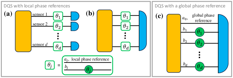
Figure 2: Models of DQS. Panels (a) and (b) show DQS schemes with local phase references. The two schemes differs by local (a) or global (b) measurements, represented by the blue semicircle(s). Green boxes are local sensors. In the simplest case, each self-referenced sensor is a two-mode device (inset) with $\theta_{j}$ being the relative phase shifts between mode $a_{j}$ and $b_{j}$, one mode providing the local phase reference. The scheme (a) shows a general configuration of DQS with local phase references. Here, the parameter $\theta_{j}$ is the relative phase shifts between modes $a_{0}$ and the mode $b_{j}$ of the $j$th local sensor. In this scheme, global measurements are necessary. In all panels, the yellow box represents schematically the probe state preparation.

Incompatibilities. The ratio between the HB and the QCRB is CarolloJSM2019

$$1\leq\frac{\mathscr{B}_{\rm H}(\rho_{\bm{\theta}},\bm{W})}{\mathscr{B}_{\rm QCR}(\rho_{\bm{\theta}},\bm{W})}\leq 1+\mathscr{R}\leq 2.$$ (5)

Here $\mathscr{R}=||i\bm{F}_{Q}^{-1}\bm{G}_{Q}||_{\infty}$, the norm $||\cdot||_{\infty}$ indicates the largest eigenvalue of a matrix, and $\bm{G}_{Q}$, defined in Eq. (C1), can be non-zero only in a multiparameter scenario. Interestingly, $0\leq\mathscr{R}\leq 1$, with $\mathscr{R}=0$ if and only if $\bm{G}_{Q}=0$ CarolloJSM2019 . The quantity $\mathscr{R}$ has been thus proposed as a figure of merit of measurement incompatibility CarolloJSM2019 ; BelliardoNJP2021 ; RazavianENTROPY2020 , see also Refs. KullJPA2020 ; LuPRL2021 for an alternative approaches based on uncertainty relations. In the case of maximal incompatibility, $\mathscr{R}=1$, the HB is at most twice the QCRB CarolloJSM2019 ; TsangPRX2020 . This factor two can be qualitatively understood within the theory of quantum local asymptotic normality KahnCMM2009 , see Ref. RafalPLA2020 for a review. According to this framework, in the limit $n\to\infty$, any quantum statistical model becomes equivalent to a Gaussian shift model and measurement incompatibility can be understood in terms of effective position and momentum displacement estimations.

For a given probe, certain combinations of the parameters cannot be estimated with the same sensitivity as others: a problem generally indicated as probe incompatibility. Assuming that the QFIM can be achieved, probe incompatibility is linked to the widely distributed spectrum of the QFIM. This is expressed by the chain of inequalities (here $n=1$, for simplicity)

$${\rm Tr}[\bm{W}\bm{C}]\geq\sum_{j}w_{j}\frac{\bm{\nu}_{j}^{\top}\bm{F}_{Q}^{-1}\bm{\nu}_{j}}{m}\geq\sum_{j}w_{j}\frac{(\bm{\nu}^{\top}_{j}\bm{\nu}_{j})^{2}}{m\,\bm{\nu}^{\top}_{j}\bm{F}_{Q}\bm{\nu}_{j}}.$$ (6)

The right-hand side provides a weak form of the QCRB that is often considered since it avoids computing the inverse of the QFIM GePRL2018 ; GessnerPRL2018 : the bound is saturated, for arbitrary $w_{j}$, if and only if $\bm{\nu}_{j}$ is an eigenstate of the QFIM MalitestaArXiv . For weight matrices of full rank, Eq. (6) can be further bounded by $d^{2}\big{[}\sum_{j=1}^{d}\tfrac{m\bm{\nu}_{j}^{\top}\bm{F}_{Q}^{-1}\bm{\nu}_{j}}{w_{j}(\bm{\nu}^{\top}_{j}\bm{\nu}_{j})^{2}}\big{]}^{-1}$ with equality if and only if $\bm{W}_{\rm opt}=\lambda\bm{F}_{Q}$. For a given $\bm{F}_{Q}$, $\bm{W}_{\rm opt}$ provides the optimal choice of weight matrix, ${\rm Tr}[\bm{W}\bm{C}]\geq{\rm Tr}[\bm{W}_{\rm opt}\bm{C}]=\lambda d/m$. Viceversa, taking an identity weight matrix, $\bm{W}=\mathbbm{1}_{d}$, corresponding to ${\rm Tr}[\bm{C}]=\sum_{j=1}^{d}\Delta^{2}\theta_{j}$ being the sum of single-parameter variances, optimal states $\rho_{\bm{\theta}}$ have a diagonal QFIM RagyPRA2016 ; NicholsPRA2018 ; SuzukiJPA2020 .

Distributed quantum sensing. Distributed quantum sensing (DQS) consists of a network of $d$ spatially-delocalized sensors. In the ideal scenario, the parameter-encoding transformations is $\bigotimes_{j=1}^{d}e^{-i\theta_{j}H_{j}}$, where the local Hamiltonians $H_{j}$ modeling each sensor commute: $[\hat{H}_{i},\hat{H}_{j}]=0$, for all $i,j=1,...,d$. This working condition has two advantages: it identifies the Hamiltonians as the generators of the local unitary evolution, $H_{j}=\mathscr{H}_{j}$, see Box. Advances in multiparameter quantum sensing and metrology, and guarantees the saturation of the QCRB for pure states and with single-copy measurements, according to Eq. (C2).

By distributing an entangled state among different sensing nodes, DQS enables the estimation of local parameters $\theta_{1},...,\theta_{d}$, or their linear combinations, with a sensitivity that surpasses what is achievable using unentangled states. DQS has been mainly explored in photonic platforms, particularly estimating multiple phase shifts across distinct optical paths. The generalization to atomic platforms includes applications such as differential interferometry CorgierQUANTUM2023 and gradient magnetometry ApellanizPRA2018 . Two main DQS architectures have been studied in the literature, differing in their phase reference configurations, as illustrated in Fig. 2.

DQS with local phase references. In this configuration, each sensor performs a relative phase measurement GePRL2018 ; MalitestaArXiv ; ZhuangPRA2018 ; PezzeARXIV2024 , see Fig. 2(a-b). The $j$th sensor comprises two modes, $a_{j}$ and $b_{j}$, with $H_{j}=(N_{j}^{(a)}-N_{j}^{(b)})/2$, $N_{j}^{(a)}$ and $N_{j}^{(b)}$ are number of particles operators, and $\theta_{j}$ is the relative phase shift among the two modes. Optimal measurements schemes can be local at each sensor, Fig 2(a), or global, Fig 2(b), requiring the recombination of the different sensing modes after phase encoding. Depending on the properties of the probe state, we recognize four possible scenarios, see Fig. 3, contingent on the utilization of mode- and/or particle-entanglement GessnerPRL2018 ; LiuNATPHOT2020 . In the following, the four possibilities are compared by using the same total number of particles, $N_{T}$, and, for simplicity, by taking $\Delta^{2}(\bm{\nu}^{\top}_{\rm ave}\bm{\theta})$ as the figure of merit, where $\bm{\nu}_{\rm ave}=\{1,...,1\}^{\top}/d$ and $\bm{\nu}^{\top}_{\rm ave}\bm{\theta}=\tfrac{1}{d}\sum_{j=1}^{d}\theta_{j}$ is the average of the $d$ phases. This combination of parameters provides the maximum sensitivity enhancement offered by entanglement. In this case, all protocols of Fig. 3 are optimized by using the same number of particles $N=N_{T}/d$ (assumed integer) in each sensor.

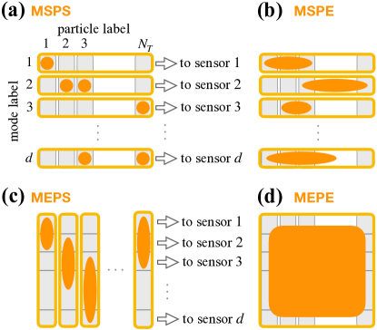
Figure 3: Quantum resources in DQS with local phase references. A DQS probe state of $N_{T}$ particles is distributed among $d$ modes. The horizontal (vertical) lines represent the particle (mode) partition of the quantum state. The probe state can be prepared as (a) mode and particle separable (MSPS), (b) mode separable and particle entangled (MSPE), (c) mode entangled and particle separable (MEPS), or (d) mode and particle entangled (MEPE). Mode (particle) entanglement is schematically illustrated by broad vertical (horizontal) ensembles encompassing multiple labels.

When the probe state is mode-separable (MS), the $d$ sensors operate independently, see Fig. 3(a) and (b). In this case, the QFIM is diagonal: the sensitivity bounds follow the single-parameter case GiovannettiNATPHOT2011 ; PezzeRMP2018 and can be saturated with local measurements at each sensor. The highest sensitivity of the mode-separable-particle-separable (MSPS) strategy of Fig. 3(a) is the standard quantum limit (SQL)

$$\Delta^{2}(\bm{\nu}^{\top}_{\rm ave}\bm{\theta})_{\rm MSPS}=\frac{1}{mNd}=\frac{1}{mN_{T}},$$ (7)

achieved with

$$\ket{\psi_{\rm MSPS}}=\bigotimes_{j=1}^{d}\bigg{(}\frac{\ket{1,0}_{j}+\ket{0,1}_{j}}{\sqrt{2}}\bigg{)}^{\otimes N}.$$ (8)

Here, $\ket{N,0}_{j}$ ($\ket{0,N}_{j}$) is a state of $N$ ($0$) particles – assumed integer – in the mode $a_{j}$ ($b_{j}$) of the $j$th sensor and $0$ ($N$) particles in the other mode, see Fig. 2(a-b). Particle entanglement, Fig. 3(b), is necessary to overcome the SQL for the estimation of each $\theta_{j}$ PezzePRL2009 . The maximum sensitivity achievable with a mode-separable-particle-entangled (MSPE) probe, is

$$\Delta^{2}(\bm{\nu}_{\rm ave}^{\top}\bm{\theta})_{\rm MSPE}=\frac{1}{mN^{2}d}=\frac{d}{mN_{T}^{2}},$$ (9)

obtained when using a product of NOON states

$$\ket{\psi_{\rm MSPE}}=\bigotimes_{j=1}^{d}\frac{\ket{N,0}_{j}+\ket{0,N}_{j}}{\sqrt{2}}.$$ (10)

Equation (9) overcomes the SQL by a factor $N$, equal to the number of particles in each sensor PezzePRL2009 ; GiovannettiNATPHOT2011 ; PezzeRMP2018 .

A mode-entangled (ME) probe establishes quantum correlations between the modes of the different sensors. The possible benefit of ME depends on whether the figure of merit ${\rm Tr}[\bm{W\bm{F}_{Q}^{-1}}]$ takes advantage of the off-diagonal elements of the QFIM. If the weight matrix $\bm{W}$ is diagonal, then MS states can enable an estimation uncertainty that is at least as small as the one that can be achieved with ME states ProctorPRL2018 , as a direct consequence of the probe incompatibility discussed previously. In contrast, ME can play a relevant role to reduce the uncertainty for the estimation of linear combinations of parameters, namely for $\bm{W}=\bm{\nu}\bm{\nu}^{T}$ ProctorPRL2018 ; GePRL2018 . In general, the saturation of the QCRB with ME states requires global measurements, as in Fig. 2(b). Overall, the QFIM is a relevant figure of merit to study the interplay of useful mode- and particle-entanglement in DQS GessnerNATCOMM2020 . The mode-entangled-particle-separable (MEPS) strategy of Fig. 3(c) is obtained by distributing independent single particles over the $d$ sensors. The corresponding sensitivity, $\Delta^{2}(\bm{\nu}^{\top}\bm{\theta})_{\rm MEPS}$ reaches the SQL, at best GessnerPRL2018 . To overcome Eq. (7), particle entanglement is necessary. The ultimate bound when using mode-entangled-particle-entangled (MEPE) states is GessnerPRL2018 ; ProctorPRL2018

$$\Delta^{2}(\bm{\nu}_{\rm ave}^{\top}\bm{\theta})_{\rm MEPE}=\frac{1}{mN^{2}d^{2}}=\frac{1}{mN_{T}^{2}},$$ (11)

which can be achieved with the multi-mode NOON-like state GessnerPRL2018 ; ProctorPRL2018

$$\ket{\psi_{\rm MEPE}}=\frac{\otimes_{j=1}^{d}\ket{N,0}_{j}+\otimes_{j=1}^{d}\ket{0,N}_{j}}{\sqrt{2}}.$$ (12)

We remark that Eq. (12) is only sensitive to the specific combination of the parameters $\bm{\nu}_{\rm ave}^{\top}\bm{\theta}$ : the different $\theta_{j}$ cannot be estimated separately and DQS reduces effectively to a single-parameter estimation problem (the QFIM is of rank-1). Equation (11) is a factor $d$ smaller than Eq. (9). This sensitivity enhancement is a direct consequence of the larger number of entangled particles LiuNATPHOT2020 : in the state Eq. (12) all $N_{T}$ particles are entangled, while only $N=N_{T}/d$ particles are entangled in the state Eq. (10).

The above results can be generalized to a arbitrary linear combinations $\bm{\nu}^{\top}\bm{\theta}$ upon optimizing the NOON-like state as in Eq. (12) and the distribution of particles in each sensor. For example, the state $(\ket{N,0}_{1}\ket{0,N}_{2}+\ket{0,N}_{1}\ket{N,0}_{2})/\sqrt{2}$ can be used to estimate the difference $\theta_{1}-\theta_{2}$ with sensitivity given by Eq. (11). For a generic $\bm{\nu}$, the maximum gain of the MEPE strategy over the MSPE one is $\mathscr{G}(\bm{\nu})=\Delta^{2}(\bm{\nu}^{\top}\bm{\theta})_{\rm MSPE}/\Delta^{2}(\bm{\nu}^{\top}\bm{\theta})_{\rm MEPE}=\lVert\bm{\nu}\rVert^{2}_{2/3}/\lVert\bm{\nu}\rVert^{2}_{1}$ ProctorPRL2018 , where $\lVert\bm{\nu}\rVert_{\gamma}=(\sum_{j=1}^{d}|\nu_{j}|^{\gamma})^{1/\gamma}$. The gain $\mathscr{G}$ ranges from one, when estimating a single parameter (e.g. $\bm{\nu}=\{1,0,...,0\}^{\top}$), to a maximum $\mathscr{G}=d$, achieved for $\bm{\nu}=\bm{\nu}_{\rm ave}$ ProctorPRL2018 ; GessnerPRL2018 ; GePRL2018 . Finally, a DQS protocol to estimate arbitrary analytical functions of $\bm{\theta}$ using ME states has been discussed in Ref. QianPRA2019 .

DQS with NOON-like (or GHZ-like, in the case of distinguishable qubits) states has been explored experimentally. The case of two qubits ($N=2$ and $d=2$) prepared in a Bell state [analogous to Eq. (12)] has been realized with photons ZhaoPRX2021 and trapped Strontium ions NicholNATURE2022 . The former experiment has demonstrated distributed sensing with unconditional (without post-selection) sensitivity overcoming the SQL by 0.92 dB. The experiment of Ref. NicholNATURE2022 has realized a quantum network of entangled atomic clocks, reporting a sensitivity beyond the SQL for the estimation of the frequency difference between two clocks. The experiment LiuNATPHOT2020 has investigated DQS using the state Eq. (12) for $d=3$ sensors and $N_{T}=6$ photons in total. This experiment has demonstrated 2.7 dB of gain over the SQL for the estimation of the average phase $(\theta_{1}+\theta_{2}+\theta_{3})/3$, also combined with a multi-round protocol. It has been also emphasized KimNATCOMM2024 that the MEPE state of Eq. (12) requires $N\geq d$ particles to estimate an equally-weighted sum of parameters. Alternative quantum states that circumvent this difficulty have been proposed and experimentally implemented with $d=4$ and $N=2$ photonic qubits KimNATCOMM2024 , reaching 2.2 dB sensitivity enhancement over the SQL. While most proof-of-principle DSQ experiments are confined to laboratory-scale setups, Refs. ZhaoPRX2021 ; KimNATCOMM2024 have demonstrated phase shift estimations over fiber distances exceeding a kilometer.

Since the NOON/GHZ-like states as in Eq. (12) are fragile and difficult to create with a large number of particles, several works have focused on DQS schemes exploiting more robust states GePRL2018 ; GessnerNATCOMM2020 . A practical strategy to generate useful ME states for DQS applications is to split a non-classical state by using a linear beam splitting network ClementsOPTICA2016 , also indicated as quantum circuit (QC) or tritter (quarter) for $d=3$ ($d=4$). As an example, Box. Advances in multiparameter quantum sensing and metrology shows a sensing scheme involving a network of Mach-Zehnder interferometers (MZIs) that uses a single non-classical state distributed by a QC. Such a splitting may introduce additional noise and losses, which limits scalability and performance of the ME sensor network. Furthermore the QC must be optimized in order to minimize the uncertainty $\Delta^{2}(\bm{\nu}^{\top}\bm{\theta})$, for a given $\bm{\nu}$. The experiment MaliaNATURE2022 has investigated the case of two atomic interferometers where a suitable four-mode spin-squeezed state generated by quantum non-demolition measurement is used to estimate the differential phase shift $\theta_{1}-\theta_{2}$ with a sensitivity overcoming the SQL by 11.6 dB. In addition, DQS using bright two-mode squeezed light in a SU(1,1) interferometer has been reported in Ref. HongARXIV2024 , estimating an optimal linear combination of $d=2$ local phase shifts with sensitivities 1.7 dB below the SQL and using local homodyne detection.

DQS with a global phase reference. The scheme of Fig. 2(c) consists of $d+1$ modes and is sensitive to the $d$ relative phase shifts $\theta_{j}$ with respect to a common phase reference. The generator of $j$th phase encoding is the number of particle operator $H_{j}=N_{j}$ [represented schematically by the green circle in Fig. 2(c)]. The scheme can be understood as a multimode MZI for the estimation of the $d$ phases, where a global measurement recombining the sensing modes is necessary. The scheme, first proposed in Ref. HumphreysPRL2013 in the framework of discrete variables, naturally involves ME and is conveniently described in the qudit formalism CiampiniSCIREP2016 , where each qudit is a single particle distributed among the $d+1$-modes. The potential advantage of DQS can emerge in the simultaneous estimation of each phase individually and is captured by the figure of merit ${\rm Tr}[\bm{C}]=\sum_{j=1}^{d}\Delta^{2}\theta_{j}$, given by the sum of estimation variances. When using the generalized NOON-like state HumphreysPRL2013

$$\ket{\psi(N_{T})}=\frac{\ket{N_{T},0,...,0}}{\sqrt{1+\sqrt{d}}}+\frac{\ket{0,N_{T},0,...,0}+...+\ket{0,...,0,N_{T}}}{\sqrt{d+\sqrt{d}}}$$ (13)

it is possible to reach

$${\rm Tr}[\bm{C}]_{\ket{\psi(N_{T})}}=\frac{d(\sqrt{d}+1)^{2}}{4N_{T}^{2}m},$$ (14)

where $\ket{N_{0},N_{1},..,N_{d}}$ is a Fock state of $N_{j}$ particles in mode $j=0,...,d$, created before phase encoding in Fig. 3(c). Equation (14) is a factor $N_{T}$ smaller than the ${\rm Tr}[\bm{C}]_{\ket{\psi(1)}^{\otimes N_{T}}}=d(\sqrt{d}+1)^{2}/(4N_{T}m)$ achieved with the MS state of $N_{T}$ qudits, namely $\ket{\psi(1)}^{\otimes N_{T}}$. Furthermore, Eq. (14) is a factor $d$ smaller (for $d\gg 1$) when compared to the ${\rm Tr}[\bm{C}]_{\rm MSPE}=d^{3}/N^{2}_{T}$ achieved with the optimal MSPE state of Fig. 3(a) HumphreysPRL2013 . The scheme of Fig. 2(c) has been also studied when using a QC for the preparation of a ME state, considering multimode Fock CiampiniSCIREP2016 as well as Gaussian NicholsPRA2018 ; OhPRR2020 states as input.

The multimode interferometer of Fig. 2(c) has been implemented experimentally in various photonic platforms, in both discrete- and continuous-variable frameworks. Integrated circuits have been used for the estimation of two PolinoOPTICA2019 and three ValeriPRR2023 optical phases with pairs of single photon Fock states. This platform has reached a sensitivity below the classical bound, also implementing various optimal sensing strategies CiminiJPJQI2024 ; CiminiPRApp2021 , see discussion below. Reference GuoNATPHYS2020 has realized the scheme of Fig. 2(c) by splitting a displaced squeezed state into $d=4$ modes with a QC. In this experiment, a strong coherent state provides the phase reference for final homodyne detection, obtained by recombining each mode with the common reference one and measuring the phase quadrature. This entangled DQS scheme reaches a higher sensitivity for the estimation of the arithmetic average of the phase shifts, $(\theta_{1}+...+\theta_{4})/4$, with respect to a sequential protocol, where the sensing nodes are interrogated with independent squeezed states and using the same total intensity of the squeezed light GuoNATPHYS2020 . Similar to the scheme of Box. Advances in multiparameter quantum sensing and metrology, a practical advantage is that the ME approach can reach a sub-SQL sensitivity while using a single squeezed state, rather than the $d$ squeezed states necessary in the separable approach. The main difference with respect to the Mach-Zehnder sensor networks is the intrinsic requirement of a global measurement scheme. The experiment HongNATCOMM2021 has demonstrated DQS using a four-mode NOON states similar to Eq. (13), with $N=2$ photons, for the estimation of $d=3$ phases. The multi-mode NOON state is recombined by a QC before final single-photon detection and the corresponding FIM is computed. The experiment demonstrated that each phase can be estimated with a sensitivity overcoming the SQL.

Optimizations. The estimation bounds discussed previously (in particular the CRB and the MIB) require a large number of measurement repetitions, $m\gg 1$, for their saturation. However, realistic scenarios are often constrained by resources – such as time and number of particles RubioPRA2020 . Therefore, optimizing the probe state and measurement setting becomes essential to maximize information acquired from each measurement, also accounting for noise, biases, and the limited operations of the device. Devising optimization strategies is particularly demanding in the multiparameter case GebhartNRP2023 .

Real-time optimization. Adaptive control protocols typically use Bayesian techniques. The prior knowledge, $P(\bm{\vartheta})$, about the parameter to be estimated is updated after each measurement outcome. The Bayes’s theorem provides the distribution $P(\bm{\vartheta}|\bm{k})=P(\bm{k}|\bm{\vartheta})P(\bm{\vartheta})/P(\bm{k})$, where $P(\bm{k}|\bm{\vartheta})$ is the likelihood function and $P(\bm{k})$ provides the normalization. The posterior $P(\bm{\vartheta}|\bm{k})$ quantifies the probability (in the sense of a degree of belief) that $\bm{\vartheta}$ equals the true value of the parameter, $\bm{\theta}$. From $P(\bm{\vartheta}|\bm{k})$, it is possible to derive the Bayesian covariance matrix,

$$\bm{C}_{B}=\int d^{d}\bm{\vartheta}P(\bm{\vartheta}|\bm{k})[\bm{\theta}-\bm{\vartheta}][\bm{\theta}-\bm{\vartheta}]^{T},$$ (15)

in analogy to Eq. (1), giving the multivariate width of the posterior around $\bm{\theta}$. While the CRB does not apply in the Bayesian setting, for a sufficiently large number of independent measurements, $m\gg 1$, the posterior becomes a multivariate normal distribution, centered at $\bm{\theta}$ and with $\bm{C}_{B}=\bm{F}^{-1}/m$ GebhartNRP2023 . The Bayesian approach allows to calculate the uncertainty associated to a specific set of outcomes and to make predictions about future measurement results, guiding the tuning of the probe state, control parameters and measurement observables. Bayesian protocols, where control phases are progressively adapted to drive the system toward optimal working point, have been implemented in a multiarm interferometer using machine learning CiminiPRApp2021 ; CiminiAP2023 and variational ValeriNPJQI2020 adaptive optimization. Reference GebhartPRApp2021 has proposed a Bayesian quantum phase estimation protocol using single qudits in the scheme of Fig. 2(c) and a multiple-interrogation protocol with real-time optimization. The main obstacles of implementing the Bayesian protocol are the required calibration of the experimental apparatus and the computational resources required for dealing with continuous $d$-dimensional posterior functions.

Off-line optimization and noise mitigation. Designing optimal quantum protocols for specific multiparameter sensing schemes is a complex task that has been only partially addressed in the literature. Efforts have been devoted to devise schemes able to overcome the trade-offs due to incompatibility. A prototypical example is the estimation of parameters $\theta_{1}$ and $\theta_{2}$ of the quadrature displacement $e^{i\theta_{1}\hat{Q}+i\theta_{2}P}$ HolevoBOOK1982 , where $P$ and $Q$ are quadrature operators. In this case, a scheme using symmetric two-mode squeezed state and specific Gaussian measurements GenoniPRA2013 can saturate HB BradshawPRA2018 and estimate simultaneously the two parameters with high precision, as demonstrated experimentally in an optical system SteinlechnerNATPHOT2013 . A further example is vector field sensing with $N_{T}$ qubits, which is relevant for magnetometry MengNATCOMM2023 . It consists in estimating the parameters $B$, $\theta$ and $\phi$ that characterize the transformation $e^{i\bm{n}\cdot\bm{J}}$, where $\bm{n}=B(\sin\theta\cos\phi,\sin\theta\sin\phi,\cos\theta)^{\top}$, $\bm{J}=(J_{x},J_{y},J_{z})$, $J_{h}=\tfrac{1}{2}\sum_{j=1}^{N_{T}}\sigma_{h}^{(j)}$ and $\sigma_{x,y,z}^{(j)}$ are Pauli operators for the $j$th spin. Optimal quantum states that saturate the QCRB have been discussed in Refs. BaumgratzPRL2016 ; HouPRL2020 . Vector field sensing has been explored experimentally with photonic qubits HouSCIADV2021 ; XiaNATCOMM2023 showing probe states and measurement schemes YuanPRL2016 overcoming incompatibility trade-offs ChenNPJQI2024 .

Complex optimization techniques for multiparameter sensing include variational methods KaubrueggerPRXQuantum2023 ; MeyerNPJQI2021 , also implemented experimentally in a multimode interferometer CiminiJPJQI2024 , machine learning approaches, which have been used to improve the performance of vector magnetometry MengNATCOMM2023 , conic programming for states and measurements HayashiNPJQI2024 , and optimal control YuanPRA2017 . Additional goals include optimizing the number of measurement repetitions and extending the range of parameter values that can be estimated with entanglement-enhanced sensitivity. Finding the optimal trade-off between precision, accuracy, bandwidth and resource consume is important in order to clarify the advantage of entangled multiparameter estimation GoreckiPRL2022 . The challenge further sharpens when including experimental imperfections and decoherence, which are central to designing practical quantum sensors SekatskiPRR2020 ; AlbarelliPRX2022 . Developing estimation protocols that are robust to noise, such as those incorporating error correction ZhuangNJP2020 ; GreckiQUANTUM2020 and noise-aware estimation algorithms GoldbergPRR2023 , is also essential to enhancing precision.

Conclusions. The recent vibrant research activity in multiparameter quantum metrology and sensing has significantly advanced our understanding – both theoretical and experimental – of a field with foundations dating back to the 1970s HolevoBOOK1982 ; HelstromBOOK1976 . Beyond its potential for groundbreaking advances in precision measurements, the simultaneous estimation of multiple parameters may serve as a bridge between quantum sensing and other quantum technologies, including simulation, cryptography, and computation. This interdisciplinary cross-fertilization remains largely unexplored, presenting opportunities for future research. From a theoretical perspective, only relatively simple sensing configurations have been investigated in details so far. It would be important to explore if more complex network geometries and entangled probe states that can provide significant advantages in the presence of imperfections and decoherence. From the experimental point of view, the challenge is to prove the quantum advantage with respect to current classical protocols in cutting-edge technological applications.

Acknowledgments. We thank Francesco Albarelli, Marco Barbieri, Animesh Datta, Rafal Demkowicz-Dobrzański, Satoya Imai, Fabio Sciarrino, and Geza Tóth for comments and suggestions. This work has been supported by the QuantERA project SQUEIS (Squeezing enhanced inertial sensing), funded by the European Union’s Horizon Europe Program and the Agence Nationale de la Recherche (ANR-22-QUA2-0006);

- (1) J. Ye and P. Zoller, “Essay : Quantum sensing with atomic, molecular, and optical platforms for fundamental physics”, Phys. Rev. Lett. 132, 190001 (2024).
- (2) P. Kómár, E. M. Kessler, M. Bishof, L. Jiang, A. S. Sørensen, J. Ye, and M. D. Lukin, “A quantum network of clocks”, Nature Physics 10, 582 (2014).
- (3) F. Albarelli, M. Barbieri, M. Genoni, and I. Gianani, “A perspective on multiparameter quantum metrology: From theoretical tools to applications in quantum imaging”, Phys. Lett. A 384, 126311 (2020).
- (4) C. L. Degen, F. Reinhard, and P. Cappellaro, “Quantum sensing”, Rev. Mod. Phys. 89, 035002 (2017).
- (5) M. A. Taylor, and W. P. Bowen, “Quantum metrology and its application in biology”, Phys. Rep. 615, 1 (2016).
- (6) N. Aslam, H. Zhou, E. K. Urbach, M. J. Turner, R. L. Walsworth, M. D. Lukin, and H. Park, “Quantum sensors for biomedical applications”, Nature Reviews Physics 5, 157 (2023).
- (7) M. R. Grace, C. N. Gagatsos, Q. Zhuang, and S. Guha, “Quantum-enhanced fiber-optic gyroscopes using quadrature squeezing and continuous-variable entanglement”, Phys. Rev. Appl. 14, 034065 (2020).
- (8) V. Gebhart, R. Santagati, A. A. Gentile, E. M. Gauger, D. Craig, N. Ares, L. Banchi, F. Marquardt, L. Pezzè, and C. Bonato, “Learning quantum systems”, Nature Reviews Physics 5, 141 (2023).
- (9) K. Bharti, A. Cervera-Lierta, T. H. Kyaw, T. Haug, S. Alperin-Lea, A. Anand, M. Degroote, H. Heimonen, J. S. Kottmann, T. Menke, W.-K. Mok, S. Sim, L.-C. Kwek, and A. Aspuru-Guzik, “Noisy intermediate-scale quantum algorithms”, Rev. Mod. Phys. 94, 015004 (2022).
- (10) S. Wehner, D. Elkouss, and R. Hanson, “Quantum internet : A vision for the road ahead”, Science 362, 1 (2018).
- (11) M. D. Vidrighin, G. Donati, M. G. Genoni, X.-M. Jin, W. S. Kolthammer, M. Kim, A. Datta, M. Barbieri, and I. A. Walmsley, “Joint estimation of phase and phase diffusion for quantum metrology”, Nature Communications 5, 3532 (2014).
- (12) V. Giovannetti, S. Lloyd, and L. Maccone, “Advances in quantum metrology”, Nature Photonics 5, 222 (2011).
- (13) L. Pezzè, A. Smerzi, M. K. Oberthaler, R. Schmied, and P. Treutlein, “Quantum metrology with nonclassical states of atomic ensembles”, Rev. Mod. Phys. 90, 035005 (2018).
- (14) C. W. Helstrom, Quantum detection and estimation theory (Academic Press, 1976).
- (15) S. M. Kay, Fundamentals of Statistical Signal Processing (Prentice-Hall, 1993).
- (16) J. Suzuki, Y. Yang, and M. Hayashi, “Quantum state estimation with nuisance parameters”, J. Phys. A 53, 453001 (2020).
- (17) S. L. Braunstein and C. M. Caves, “Statistical distance and the geometry of quantum states”, Phys. Rev. Lett. 72, 3439 (1994).
- (18) J. Liu, H. Yuan, X.-M. Lu, and X. Wang, “Quantum Fisher Information matrix and multiparameter estimation”, J. Phys. A 53, 023001 (2019).
- (19) M. Gessner, L. Pezzè, and A. Smerzi, “Sensitivity bounds for multiparameter quantum metrology”, Phys. Rev. Lett. 121, 130503 (2018).
- (20) T. J. Proctor, P. A. Knott, and J. A. Dunningham, “Multiparameter estimation in networked quantum sensors”, Phys. Rev. Lett. 120, 080501 (2018).
- (21) W. Ge, K. Jacobs, Z. Eldredge, A. V. Gorshkov, and M. Foss-Feig, “Distributed quantum metrology with linear networks and separable inputs”, Phys. Rev. Lett. 121, 043604 (2018).
- (22) H. Chen, Y. Chen, and H. Yuan, “Information geometry under hierarchical quantum measurement”, Phys. Rev. Lett. 128, 250502 (2022).
- (23) A. S. Holevo, Probabilistic and Statistical Aspects of Quantum Theory (Elsevier Science Ltd, 1982).
- (24) H. Nagaoka, “A new approach to cramer-rao bounds for quantum state estimation”, in Asymptotic Theory of Quantum Statistical Inference : Selected Papers, edited by M. Hayashi (World Scientific, Singapore, 2005), pp. 100–112.
- (25) R. Demkowicz-Dobrzański, W. Górecki, and M. Guţă, “Multi-parameter estimation beyond quantum Fisher in- formation”, J. Phys. A 53, 363001 (2020).
- (26) J. Suzuki, “Information geometrical characterization of quantum statistical models in quantum estimation theory”, Entropy 21, 7 (2019).
- (27) E. Roccia, I. Gianani, L. Mancino, M. Sbroscia, F. Somma, M. G. Genoni, and M. Barbieri, “Entangling measurements for multiparameter estimation with two qubits”, Quantum Sci. Technol. 3, 01LT01 (2017).
- (28) L. O. Conlon, T. Vogl, C. D. Marciniak, I. Pogorelov, S. K. Yung, F. Eilenberger, D. W. Berry, F. S. Santana, R. Blatt, T. Monz, P. K. Lam, and S. M. Assad, “Approaching optimal entangling collective measurements on quantum computing platforms”, Nature Physics 19, 351 (2023).
- (29) P. Horodecki, L. Rudnicki, and K. Życzkowski, “Five open problems in quantum information theory”, PRX Quantum 3, 010101 (2022).
- (30) L. O. Conlon, J. Suzuki, P. K. Lam, and S. M. Assad, “Efficient computation of the Nagaoka–Hayashi bound for multiparameter estimation with separable measurements”, npj Quantum Information 7, 110 (2021).
- (31) M. Hayashi and Y. Ouyang, “Tight Cramér-Rao type bounds for multiparameter quantum metrology through conic programming”, Quantum 7, 1094 (2023).
- (32) M. Hayashi and K. Matsumoto, “Asymptotic performance of optimal state estimation in qubit system”, J. Math. Phys. 49, 102101 (2008).
- (33) J. Suzuki, “Explicit formula for the Holevo bound for two-parameter qubit-state estimation problem”, J. Math. Phys. 57, 042201 (2016).
- (34) K. Matsumoto, “A new approach to the Cramér-Rao-type bound of the pure-state model”, J. Phys. A 35, 3111 (2002).
- (35) M. Bradshaw, P. K. Lam, and S. M. Assad, “Ultimate precision of joint quadrature parameter estimation with a Gaussian probe”, Phys. Rev. A 97, 012106 (2018).
- (36) J. S. Sidhu, Y. Ouyang, E. T. Campbell, and P. Kok, “Tight bounds on the simultaneous estimation of incompatible parameters”, Phys. Rev. X 11, 011028 (2021).
- (37) F. Albarelli, J. F. Friel, and A. Datta, “Evaluating the Holevo Cramér-Rao bound for multiparameter quantum metrology”, Phys. Rev. Lett. 123, 200503 (2019).
- (38) J. Kahn and M. Guţă, “Local asymptotic normality for finite dimensional quantum systems”, Commun. Math. Phys. 289, 597 (2009).
- (39) K. Yamagata, A. Fujiwara, and R. D. Gill, “Quantum local asymptotic normality based on a new quantum likelihood ratio”, Annals of Statistics 41, 2197 (2013).
- (40) Y. Yang, G. Chiribella, and M. Hayashi, “Attaining the ultimate precision limit in quantum state estimation”, Commun. Math. Phys. 368, 223 (2019).
- (41) S. Ragy, M. Jarzyna, and R. Demkowicz-Dobrzański, “Compatibility in multiparameter quantum metrology”, Phys. Rev. A 94, 052108 (2016).
- (42) L. O. Conlon, J. Suzuki, P. K. Lam, and S. M. Assad, “The gap persistence theorem for quantum multipara- meter estimation”, arXiv:2208.07386.
- (43) J. Yang, S. Pang, Y. Zhou, and A. N. Jordan, “Optimal measurements for quantum multiparameter estimation with general states”, Phys. Rev. A 100, 032104 (2019).
- (44) L. O. Conlon, J. Suzuki, P. K. Lam, and S. M. Assad, “Role of the extended Hilbert space in the attainability of the Quantum Cramér-Rao bound for multiparameter estimation”, arXiv:2404.01520.
- (45) L. Pezzè, M. A. Ciampini, N. Spagnolo, P. C. Hum- phreys, A. Datta, I. A. Walmsley, M. Barbieri, F. Sciar- rino, and A. Smerzi, “Optimal measurements for simultaneous quantum estimation of multiple phases”, Phys. Rev. Lett. 119, 130504 (2017).
- (46) M. Tsang, F. Albarelli, and A. Datta, “Quantum semiparametric estimation”, Phys. Rev. X 10, 031023 (2020).
- (47) A. Carollo, B. Spagnolo, A. A. Dubkov, and D. Valenti, “On quantumness in multi-parameter quantum estimation”, J. Stat. Mech. 2019, 094010 (2019).
- (48) F. Belliardo and V. Giovannetti, “Incompatibility in quantum parameter estimation”, New J. Phys. 23, 063055 (2021).
- (49) S. Razavian, M. G. A. Paris, and M. G. Genoni, “On the quantumness of multiparameter estimation problems for qubit systems”, Entropy 22, 11 (2020).
- (50) I. Kull, P. A. Guérin, and F. Verstraete, “Uncertainty and trade-offs in quantum multiparameter estimation”, J. Phys. A 53, 244001 (2020).
- (51) X.-M. Lu and X. Wang, “Incorporating Heisenberg’s uncertainty principle into quantum multiparameter estimation”, Phys. Rev. Lett. 126, 120503 (2021).
- (52) M. Malitesta, A. Smerzi, and L. Pezzè, “Distributed quantum sensing with squeezed-vacuum light in a configurable network of Mach-Zehnder interferometers”, Phys. Rev. A 108, 032621 (2021).
- (53) R. Nichols, P. Liuzzo-Scorpo, P. A. Knott, and G. Adesso, “Multiparameter Gaussian quantum metrology”, Phys. Rev. A 98, 012114 (2018).
- (54) R. Corgier, M. Malitesta, A. Smerzi, and L. Pezzè, “Quantum-enhanced differential atom interferometers and clocks with spin-squeezing swapping”, Quantum 7, 965 (2023).
- (55) I. Apellaniz, I. n. Urizar-Lanz, Z. Zimborás, P. Hyllus, and G. Tóth, “Precision bounds for gradient magnetometry with atomic ensembles”, Phys. Rev. A 97, 053603 (2018).
- (56) Q. Zhuang, Z. Zhang, and J. H. Shapiro, “Distributed quantum sensing using continuous-variable multipartite entanglement”, Phys. Rev. A 97, 032329 (2018).
- (57) L. Pezzè and A. Smerzi, “Distributed quantum multiparameter estimation with optimal local measurements”, arXiv:2405.18404.
- (58) L.-Z. Liu, Y.-Z. Zhang, Z.-D. Li, R. Zhang, X.-F. Yin, Y.-Y. Fei, L. Li, N.-L. Liu, F. Xu, Y.-A. Chen, and J.-W. Pan, “Distributed quantum phase estimation with entangled photons”, Nature Photonics 15, 137 (2021).
- (59) L. Pezzé and A. Smerzi, “Entanglement, nonlinear dynamics, and the Heisenberg limit”, Phys. Rev. Lett. 102, 100401 (2009).
- (60) M. Gessner, A. Smerzi, and L. Pezzè, “Multiparameter squeezing for optimal quantum enhancements in sensor networks”, Nature Communications 11, 3817 (2020).
- (61) K. Qian, Z. Eldredge, W. Ge, G. Pagano, C. Monroe, J. V. Porto, and A. V. Gorshkov, “Heisenberg-scaling measurement protocol for analytic functions with quantum sensor networks”, Phys. Rev. A 100, 042304 (2019).
- (62) S.-R. Zhao, Y.-Z. Zhang, W.-Z. Liu, J.-Y. Guan, W. Zhang, C.-L. Li, B. Bai, M.-H. Li, Y. Liu, L. You, J. Zhang, J. Fan, F. Xu, Q. Zhang, and J.-W. Pan, “Field demonstration of distributed quantum sensing without post-selection”, Phys. Rev. X 11, 031009 (2021).
- (63) B. C. Nichol, R. Srinivas, D. P. Nadlinger, P. Drmota, D. Main, G. Araneda, C. J. Ballance, and D. M. Lucas, “An elementary quantum network of entangled optical atomic clocks”, Nature 609, 689 (2022).
- (64) D.-H. Kim, S. Hong, Y.-S. Kim, Y. Kim, S.-W. Lee, R. C. Pooser, K. Oh, S.-Y. Lee, C. Lee, and H.-T. Lim, “Distributed quantum sensing of multiple phases with fewer photons”, Nature Communications 15, 266 (2024).
- (65) B. K. Malia, Y. Wu, J. Martínez-Rincón, and M. A. Kasevich, “Distributed quantum sensing with mode-entangled spin-squeezed atomic states”, Nature 612, 661 (2022).
- (66) C. Oh, C. Lee, S. H. Lie, and H. Jeong, “Optimal distributed quantum sensing using Gaussian states”, Phys. Rev. Research 2, 023030 (2020).
- (67) Y. Xia, W. Li, W. Clark, D. Hart, Q. Zhuang, and Z. Zhang, “Demonstration of a reconfigurable entangled radio-frequency photonic sensor network”, Phys. Rev. Lett. 124, 150502 (2020).
- (68) W. R. Clements, P. C. Humphreys, B. J. Metcalf, W. S. Kolthammer, and I. A. Walmsley, “Optimal design for universal multiport interferometers”, Optica 3, 1460 (2016).
- (69) S. Hong, M. A. Feldman, C. E. Marvinney, D. Lee, C. Lee, M. T. Febbraro, A. M. Marino, and R. C. Pooser, “Quantum enhanced distributed phase sensing with a truncated SU(1,1) interferometer”, arXiv:2403.17119.
- (70) P. C. Humphreys, M. Barbieri, A. Datta, and I. A. Walmsley, “Quantum enhanced multiple phase estimation”, Phys. Rev. Lett. 111, 070403 (2013).
- (71) M. A. Ciampini, N. Spagnolo, C. Vitelli, L. Pezzè, A. Smerzi, and F. Sciarrino, “Quantum-enhanced multiparameter estimation in multiarm interferometers”, Scientific Reports 6, 28881 (2016).
- (72) E. Polino, M. Riva, M. Valeri, R. Silvestri, G. Corrielli, A. Crespi, N. Spagnolo, R. Osellame, and F. Sciarrino, “Experimental multiphase estimation on a chip”, Optica 6, 288 (2019).
- (73) M. Valeri, V. Cimini, S. Piacentini, F. Ceccarelli, E. Polino, F. Hoch, G. Bizzarri, G. Corrielli, N. Spagnolo, R. Osellame, and F. Sciarrino, “Experimental multiparameter quantum metrology in adaptive regime”, Phys. Rev. Research 5, 013138 (2023).
- (74) V. Cimini, M. Valeri, S. Piacentini, F. Ceccarelli, G. Corrielli, R. Osellame, N. Spagnolo, and F. Sciar- rino, “Variational quantum algorithm for experimental photonic multiparameter estimation”, npj Quantum Information 10, 26 (2024).
- (75) V. Cimini, E. Polino, M. Valeri, I. Gianani, N. Spagnolo, G. Corrielli, A. Crespi, R. Osellame, M. Barbieri, and F. Sciarrino, “Calibration of multiparameter sensors via machine learning at the single-photon level”, Phys. Rev. Appl. 15, 044003 (2021).
- (76) X. Guo, C. R. Breum, J. Borregaard, S. Izumi, M. V. Larsen, T. Gehring, M. Christandl, J. S. Neergaard-Nielsen, and U. L. Andersen, “Distributed quantum sensing in a continuous-variable entangled network”, Nature Physics 16, 281 (2020).
- (77) S. Hong, J. ur Rehman, Y.-S. Kim, Y.-W. Cho, S.-W. Lee, H. Jung, S. Moon, S.-W. Han, and H.-T. Lim, “Quantum enhanced multiple-phase estimation with multi-mode n00n states”, Nature Communications 12, 5211 (2021).
- (78) J. Rubio and J. Dunningham, “Bayesian multiparameter quantum metrology with limited data”, Phys. Rev. A 101, 032114 (2020).
- (79) V. Cimini, M. Valeri, E. Polino, S. Piacentini, F. Ceccarelli, G. Corrielli, N. Spagnolo, R. Osellame, and F. Sciarrino, “Deep reinforcement learning for quantum multiparameter estimation”, Advanced Photonics 5, 016005 (2023).
- (80) M. Valeri, E. Polino, D. Poderini, I. Gianani, G. Corrielli, A. Crespi, R. Osellame, N. Spagnolo, and F. Sciarrino, “Experimental adaptive bayesian estimation of multiple phases with limited data”, npj Quantum Information 6, 92 (2020).
- (81) V. Gebhart, A. Smerzi, and L. Pezzè, “Bayesian quantum multiphase estimation algorithm”, Phys. Rev. Applied 16, 014035 (2021).
- (82) M. G. Genoni, M. G. A. Paris, G. Adesso, H. Nha, P. L. Knight, and M. S. Kim, “Optimal estimation of joint parameters in phase space”, Phys. Rev. A 87, 012107 (2013).
- (83) S. Steinlechner, J. Bauchrowitz, M. Meinders, H. Müller-Ebhardt, K. Danzmann, and R. Schnabel, “Quantum-dense metrology”, Nature Photonics 7, 626 (2013).
- (84) X. Meng, Y. Zhang, X. Zhang, S. Jin, T. Wang, L. Jiang, L. Xiao, S. Jia, and Y. Xiao, “Machine learning assisted vector atomic magnetometry”, Nature Communications 14, 6105 (2023).
- (85) T. Baumgratz and A. Datta, “Quantum enhanced estimation of a multidimensional field”, Phys. Rev. Lett. 116, 030801 (2016).
- (86) Z. Hou, Z. Zhang, G.-Y. Xiang, C.-F. Li, G.-C. Guo, H. Chen, L. Liu, and H. Yuan, “Minimal tradeoff and ultimate precision limit of multiparameter quantum magnetometry under the parallel scheme”, Phys. Rev. Lett. 125, 020501 (2020).
- (87) Z. Hou, J.-F. Tang, H. Chen, H. Yuan, G.-Y. Xiang, C.-F. Li, and G.-C. Guo, “Zero-trade-off multiparameter quantum estimation via simultaneously saturating multiple Heisenberg uncertainty relations”, Science Advances 7, 2986 (2021).
- (88) B. Xia, J. Huang, H. Li, H. Wang, and G. Zeng, “Toward incompatible quantum limits on multiparameter estimation”, Nature Communications 14, 1021 (2023).
- (89) H. Yuan, “Sequential feedback scheme outperforms the parallel scheme for Hamiltonian parameter estimation”, Phys. Rev. Lett. 117, 160801 (2016).
- (90) H. Chen, L. Wang, and H. Yuan, “Simultaneous measurement of multiple incompatible observables and tradeoff in multiparameter quantum estimation”, npj Quantum Information 10, 98 (2024).
- (91) R. Kaubruegger, A. Shankar, D. V. Vasilyev, and P. Zoller, “Optimal and variational multiparameter quantum metrology and vector-field sensing”, PRX Quantum 4, 020333 (2023).
- (92) J. J. Meyer, J. Borregaard, and J. Eisert, “A variational toolbox for quantum multi-parameter estimation”, npj Quantum Information 7, 89 (2021).
- (93) M. Hayashi and Y. Ouyang, “Finding the optimal probe state for multiparameter quantum metrology using conic programming”, npj Quantum Information 10, 111 (2024).
- (94) J. Liu and H. Yuan, “Control-enhanced multiparameter quantum estimation”, Phys. Rev. A 96, 042114 (2017).
- (95) W. Górecki and R. Demkowicz-Dobrzański, “Multiple-phase quantum interferometry : Real and apparent gains of measuring all the phases simultaneously”, Phys. Rev. Lett. 128, 040504 (2022).
- (96) F. Albarelli and R. Demkowicz-Dobrzański, “Probe incompatibility in multiparameter noisy quantum metrology”, Phys. Rev. X 12, 011039 (2022).
- (97) P. Sekatski, S. Wölk, and W. Dür, “Optimal distributed sensing in noisy environments”, Phys. Rev. Res. 2, 023052 (2020).
- (98) Q. Zhuang, J. Preskill, and L. Jiang, “Distributed quantum sensing enhanced by continuous-variable error correction”, New J. Phys. 22, 022001 (2020).
- (99) W. Górecki, S. Zhou, L. Jiang, and R. Demkowicz-Dobrzański, “Optimal probes and error-correction schemes in multi-parameter quantum metrology”, Quantum 4, 288 (2020).
- (100) A. Z. Goldberg, K. Heshami, and L. L. Sánchez-Soto, “Evading noise in multiparameter quantum metrology with indefinite causal order”, Phys. Rev. Res. 5, 033198 (2023).