Back-Reaction of Super-Hubble Fluctuations, Late Time Tracking and Recent Observational Results
Abstract
Previous studies suggested that the back-reaction of super-Hubble cosmological fluctuations could lead to a dynamical relaxation of the cosmological constant. Moreover, this mechanism appears to be self-regulatory, potentially leading to an oscillatory behavior in the effective dark energy. Such an effect would occur in any cosmological model with super-Hubble matter fluctuations, including the standard CDM model, without the need for additional mechanisms.
The recent DESI data, which supports the possibility of dynamical dark energy, has renewed interest in exploring scenarios leading to such oscillatory behavior. In this work we propose a parametrization to account for the impact of super-Hubble fluctuations on the background energy density of the Universe. We model the total effective cosmological constant as the sum of a constant piece and an oscillating contribution. We perform a preliminary comparison of the background dynamics of this model with the recent radial BAO data from DESI. We also discuss the status of the tension problem in this model. While this analysis serves as a first step in testing the scenario, we emphasize the importance of considering this effect, as it is naturally expected to be present and could offer valuable insights in light of the recent observational data.
I Introduction
In the standard framework of cosmology, the CDM model, the Dark Energy (DE) component, which comprises the majority of today’s cosmological energy density, is parametrized by a positive cosmological constant term, , in the Einstein equations. Despite its apparent simplicity, this interpretation faces conceptual problems. In addition to some well known problems, such as the cosmological constant problem, the coincidence problem and the Hubble tension problem, several works in the literature have been pointing to an instability of a de Sitter phase. In particular, there are indications that a de Sitter space could be unstable due to infrared (IR) effects Polyakov:2012uc ; Polyakov:2007mm ; Mazur:1986et ; Mottola:1985qt ; Mottola:1984ar ; Tsamis:1994ca 111In the context of String Theoriy there have also been indications that it is not possible to obtaine a stable de Sitter phase Obied:2018sgi ; Dvali:2014gua ; Danielsson:2018ztv ; Dasgupta:2018rtp , and the recently suggested “Trans-Planckian Censorship Criterion” Bedroya:2019snp ; Bedroya:2019tba ; Brandenberger:2021pzy implies that a positive cosmological constant is not consistent from an effective field theory point of view.. Already in the work of Ref. Tsamis:1992sx ; Tsamis:1996qq it has been suggested that the reason that our universe is not inflating today is that IR processes in pure quantum gravity (no matter) tend to screen the bare . However, the authors of Tsamis:1996qq found that these effects become important only after perturbation theory has broken down. In 1997, in the work of Ref.Abramo:1997hu the back-reaction of super-Hubble modes of cosmological perturbations induced by matter were studied, finding that the effective energy density associated with these modes would counteract any pre-existing (see also Finelli:2001bn ; Finelli:2003bp ; Marozzi:2006ky ). Later, in 1999, in the work of Brandenberger:1999su it was speculated that this dynamical relaxation mechanism for could be self-regulating 222Note also the related “Everpresent Lambda” scenario, which was proposed by drawing on ideas from causal set theory and unimodular gravity, and which leads to an effective fluctuating cosmological “constant”, see Refs.Ahmed:2002mj ; Das:2023hbw ; Das:2023rvg , for instance. . A crucial question is whether this back-reaction effect can be locally measured Unruh:1998ic ; Geshnizjani:2002wp ; Abramo:2001dc . Recent works have shown that super-Hubble fluctuation modes can in fact modify the parameters of a local Friedmann cosmology in the context of a more realistic scenario with more than one matter field, admitting entropy fluctuations (in this context see the works of Refs Geshnizjani:2003cn ; Marozzi:2012tp ; Finelli:2011cw ; Gasperini:2009wp ; Gasperini:2009mu ; Marozzi:2010qz ; Marozzi:2011zb ; Abramo:2001dd ; Losic:2005vg ; Losic:2006ht ; Brandenberger:2004ix ; Afshordi:2000nr ; Comeau:2023gxk ; Comeau:2023euf ) 333In the context of the back-reaction of sub-Hubble cosmological fluctuations, a recent analysis can be found, for instance, in Ref.Giani:2024nnv . In the work of Brandenberger:2018fdd the analysis was extended beyond perturbation theory, showing that the locally measured Hubble expansion rate indeed obtains a negative contribution from the back-reaction of super-Hubble fluctuations, whose amplitude grows in time. This supports the suggestion that (quasi) de Sitter space-times are unstable, and that this back-reaction mechanism might lead to a dynamical relaxation of the cosmological constant. As first speculated in Ref.Brandenberger:1999su , this is expected to lead to an effective dark energy density which oscillates in time around the dominant matter density.
The quest for understanding the nature and dynamics of the accelerated expansion of the Universe became even more interesting recently with the improvement in the measurements of the expansion history, which are increasingly allowing us to constrain the expansion history of the Universe. More recently, the Dark Energy Spectroscopic Instrument (DESI) Year 1 results were released DESI:2024uvr ; DESI:2024lzq , officially marking the start of the Stage IV DE era. The cosmological results stem from measurements of baryon acoustic oscillations (BAO) in galaxy, quasar and Lyman- forest tracers. The DESI results, when combined with a number of external probes, provide intriguing hints for a dynamical, time-evolving DE component DESI:2024mwx ; DESI:2024aqx ; DESI:2024kob . 444See, however, Payeur:2024dnq for caveats. These hints may have enormous implications for the understanding of the nature of DE.
In light of these results, recent works, among them Jiang:2024xnu and Escamilla:2024fzq , have pointed to signals, from late-time cosmological data, of oscillatory/non-monotonic features in the shape of the expansion rate at low redshifts. The possibility of an oscillating dark energy has already been addressed in earlier works, as for instance in RefsZhao:2017cud ; Tamayo:2019gqj ; Rubano:2003er ; Linder:2005dw ; Feng:2004ff ; Nojiri:2006ww ; Kurek:2007bu ; Jain:2007fa ; Saez-Gomez:2008mkj ; Kurek:2008qt ; Pace:2011kb ; Pan:2017zoh ; Panotopoulos:2018sso ; Rezaei:2019roe ; Yao:2022jrw ; Rezaei:2024vtg ; Tian:2019enx DESI:2024kob ; Adil:2023exv ; Mbonye:2022cnf ; Mbonye:2024mss ]. In Ref.Escamilla:2024fzq , in light of the recent cosmological data, twelve different parametrizations for an oscillatory dark energy equation of state were analyzed, among them the ones proposed in Refs. Linder:2005dw ; Feng:2004ff ; Pan:2017zoh ; Zhao:2005vj . This analysis demonstrated that all the oscillating DE parametrizations considered provided a better fit to the data when compared to the cosmological constant, although in the Bayesian evidence analysis they are penalized due to the additional free parameter. In a similar context, in the work of Ref.Jiang:2024xnu , the late-time expansion history was reconstructed in a way, according to the authors, to be “as model-independent and non-parametric as possible”. In their first reconstruction, using DESI+PantheonPlus data, two features in the unnormalized expansion rate, were identified, a bump at redshift , and a depression at (both features were absent when replacing the DESI dataset with the older SDSS one). In spite of the higher number of unique redshifts, the effective volume covered by DESI is still smaller than the one of SDSS, so whether the abovementioned features are real or due to sample variance fluctuations is something expected to be clarified with the upcoming releases from DESI. On the other hand, the depression feature was noticeable in both the DESI+PantheonPlus and DESI+Union3 reconstructions, but not in the DESI+DESY5 one 555In addition to the upcoming releases from DESI, the presence of this feature can also be checked by future SNeIa samples.. For more information on the reconstruction methods see Ref.Jiang:2024xnu . While the Chevallier-Polarski-Linder (CPL) fit, the parametrization usually considered when interpreting DESI data, is able to partially capture one of these features, it cannot fit both, since the model does not have sufficient complexity. The authors of Jiang:2024xnu conclude that fitting both features requires an oscillatory/non-monotonic behavior of the Hubble expansion rate.
While a more conclusive result will need to wait for more precise future data, we believe it is important to already now further investigate theoretical mechanisms that could account for a non-monotonic dynamical behavior of DE. As discussed above, the back-reaction effect of super-Hubble fluctuations is one mechanism that could naturally lead to an oscillatory behavior for the dark energy density, and consequently for the Hubble parameter, without the need for extra ingredients beyond the standard CDM model. This back-reaction effect is present in any cosmological model whenever entropic super-Hubble cosmological fluctuations are present, not relying on any extra ingredients. We believe that, in light of the new observational results, it is important not to neglect the possible presence of such a mechanism.
In the present work we propose a parametrization to account for the back-reaction effect of super-Hubble fluctuations by means of an oscillating effective energy density component. This may provide a full non-perturbative description of the back-reaction effect. We then analyze such a model considering data from the radial component of the Baryon Acoustic Oscillations from the recent DESI data. We compute the Hubble parameter at low redshifts as predicted by this model, and compare the result to the recent DESI data in order to estimate the maximum amplitude of the oscillations allowed by the data. We also analyze the predictions of the model for the effective dark energy equation of state, for the deceleration parameter, and for .
While our study can be considered to be a first-step analysis limited to background quantities, aiming only to highlight the importance of not neglecting the back-reaction mechanism, the scenario has the advantage of avoiding the need to make extra suppositions about a new matter source of DE. Nevertheless, in order to obtain more conclusive results, it is necessary to further analyze the predictions of the model, in particular taking into account the induced cosmological perturbations. This will allow us to test the model using additional BAO data beyond only the radial component, as well as using further data from other cosmological sources. This analysis is left for a future work.
The paper is organized as follows: In Section 2 we propose a new parametrization to describe the back-reaction of super-Hubble fluctuations in the late universe. In Section 3 we discuss the data analysis methods which we use to compare our model predictions with the recent DESI results. In Section 4 we present our results and we conclude in Section 5.
II A Model for the Back-Reaction of Super-Hubble fluctuations
The Einstein field equations, as its well known, are highly nonlinear. Even at a classical level fluctuations at second order affect the background. This effect is called back-reaction. Matter fluctuations induce metric fluctuations through the Einstein equations. These metric fluctuations also back-react on the homogeneous background metric. The full evolution of the metric is governed by the Einstein equations,
| (1) |
where is the Einstein tensor of the metric , is Newton’s gravitational constant and is the energy-momentum tensor of matter.
Metric and matter (taken for simplicity to be a scalar matter field ) can be written, at linear order in the amplitude of cosmological fluctuations, as
| (2) |
and
| (3) |
In the absence of anisotropic stress, the scalar metric fluctuation variables and in eq.2 are equal. To write the metric, we have chosen a particular coordinate system (longitudinal gauge) 666See e.g. Mukhanov:1990me for a review of the theory of cosmological perturbations.. In Eq. 2 is the background metric of the constant time hypersurfaces. We assume vanishing spatial curvature and then . In the above equations, the background metric is given by the scale factor and the background matter by . We will only consider here the effect of scalar metric fluctuations.
In order to see how the linear fluctuations affect the background, we substitute the ansatz 2 and 3 into the Einstein equations and expand to second order. The zero’th order terms satisfy the background equations. The linear terms are assumed to obey the linear perturbation equations. In this case, the Einstein equations are not satisfied at quadratic order. Back-reaction is a way to correct for this at quadratic order. The quadratic terms on the left hand side of 1 can be moved to the right hand side of the equation, where they form an effective energy-momentum tensor when combined with the quadratic terms in Abramo:1997hu ; Mukhanov:1996ak ,
| (4) |
where the superscript (2) indicates the order of the terms.
At second order, the linear perturbations modify the background metric. This effect can be described by introducing a modified background metric
| (5) |
where the first term is the original background metric and the second reflects the quadratic corrections to the background.
By taking the spatial average of the Einstein equation 1, expanded to second order, we can describe the corrections to the background. Following the method proposed in Abramo:1997hu ; Mukhanov:1996ak (and reviewed in Brandenberger:2002sk ) we can write the resulting equation in the form,
| (6) |
where the first term on the right hand side of the equation is the contribution of the background matter field to . Improved studies of the back-reaction of super-Hubble fluctuations focus on physically measurable quantities such as the spatial average of the local Hubble expansion rate Geshnizjani:2003cn ; Marozzi:2012tp ; Finelli:2011cw ; Gasperini:2009wp ; Gasperini:2009mu ; Marozzi:2010qz ; Marozzi:2011zb ; Abramo:2001dd ; Losic:2005vg ; Losic:2006ht ; Brandenberger:2004ix ; Afshordi:2000nr , and even beyond perturbation theory Brandenberger:2018fdd . Some of these results have pointed to a self adjusting mechanism for the cosmological constant, as first discussed in Brandenberger:1999su .
The origin of the self-adjusting mechanism for the relaxation of the cosmological constant is as follows Brandenberger:1999su .: in an accelerating phase, fluctuation modes exit the Hubble radius and freeze out. Cosmological perturbations induced by super-Hubble matter fluctuations contribute to the effective energy-momentum tensor like a negative cosmological constant (negligible kinetic and tension energies leading to an effective equation of state , and negative effective energy density - negative since matter induces a potential well and the negativity of the gravitational energy overwhelms the positivity of the matter energy for super-Hubble modes). This will induce a decrease in the effective cosmological constant by counteracting the effect of the pre-existing . But once the energy density in the effective cosmological constant has fallen below that of matter, accelerated expansion will stop, modes will re-enter the Hubble radius. The decrease in will stop, and soon (within a fraction of the Hubble expansion time), will again dominate, leading to a new period of acceleration which, in turn, leads to a renewed buildup of the back-reaction effect. This cycle implies an oscillatory behavior in the effective energy density associated to the back-reaction mechanism.
In light of this, we propose here the following parametrization for the effective energy density associated to the back-reaction of super-Hubble fluctuations:
| (7) |
where is a dimensionless amplitude, is the frequency of the oscillation, is a phase and is the background density of matter. The term in the above equation can be written in terms of the redshift as , with being a constant, which we expect to have an order of magnitude not much smaller or bigger than one since the typical time scale of oscillations is expected to be set by the Hubble time. This ansatz expresses the idea that, after the time of equal matter and radiation, the back-reaction term should track the energy density of matter. A priori it is expected that the amplitude should be time-dependent. However, in the present work, we will focus in the late time predictions, since we are going to analyze our model in light of data from . For this small redshift interval we believe it is reasonable to consider as a good approximation. Therefore in the rest of the paper we are going to consider the following expression for the effective density from the back-reaction effect, .
This contribution of the energy density from the back-reaction effect is added to the total energy of the universe, in such a way that the first Friedmann equation can be written as,
| (8) |
where we have kept a bare cosmological constant term . We will set the speed of light to one in the following.
By substituting Eq.7 in the above equation, we can write the first Friedmann equation as follows,
| (9) |
where 777The subscripts indicate the quantities at the present time.
| (10) | |||||
Another important quantity to be analyzed is the deceleration parameter, which must show a transition from a decelerated regime to the accelerated one as the dark energy starts dominating. The deceleration parameter is where the prime indicates derivative with respect to the redshift. By using the above equation, we obtain for the deceleration parameter the following expression,
| (11) |
Concerning the phase , we will chose it in a way that the back-reaction mechanism begins at a redshift with , when it starts building up. This choice is reasonable since we are taking the back-reaction energy density as being proportional to the matter energy density, and before recombination it would rather track the radiation component.
We can now compute the equation of state associated to the back-reaction effective fluid. The continuity equation is not valid in the usual form for this fluid, since there is an energy transfer from the cosmological fluctuations to this effective component Abramo:1997uy . In this case, in order to obtain , we can consider the second Friedmann equation for the total fluid (considering all the components of the Universe),
| (12) |
By isolating in the above equation and considering that , we obtain the following expression for the equation of state,
| (13) |
In Section IV we will illustrate the behavior of the Hubble parameter at low redshifts, the deceleration parameter and the effective equation of state for chosen values of the frequency and amplitude in Eq.7.
In this work we will restrict our analysis to the background dynamics. We then do not need to make extra assumptions on the cosmological model at perturbative level. A further discussion of the perturbative quantities of the model is left for a future work. While this allow us to make more general predictions concerning the back-reaction mechanism, we consider this study to be a preliminary analysis. In order to obtain more conclusive results, it would be necessary to go beyond the background analysis and test the model with a more complete cosmological dataset. However the expression above already provide us some insights in light of specific datasets, as for instance the radial component of BAO, which we are going to discuss in the next section.
III Methods and Data Analysis
The baryon acoustic oscillation (BAO) method is one of the main methods already developed to measure the expansion history of the Universe (for a more complete discussion see for instance Weinberg:2013agg ; Chen:2024tfp ; DESI:2024uvr ). In the pre-recombination Universe, acoustic oscillations in the baryon-photon fluid imprinted a characteristic scale on the clustering of matter, which manifests itself as a bump in the two-point correlation function of matter (or as a series of oscillations in the power spectrum). The comoving scale of this feature, is given by the sound horizon at the end of the baryon drag epoch, . This quantity depends on the photon and baryon content of the universe at this epoch, and it is well constrained by CMB measurements. The BAO feature can be traced by galaxies, quasars, and the Lyman- forest.
The BAO signature can be measured in two ways: one can use the angular diameter distance to determine the physical length scale corresponding to a certain angle on the sky of the observer, or one can use the difference in redshift to infer some physical radial distance. Therefore, there are measurements of the apparent size of the BAO standard ruler perpendicular and parallel to the line of sight, allowing one to constrain the angular diameter distance and the Hubble parameter , respectively. If the Hubble parameter of our Universe is actually different than the one predicted by the model considered, then there will be differences in the radial BAO scale.
We can therefore decompose the BAO locations into transverse and line-of-sight dilation parameters, which are denoted by the Alcock-Paczynski-like dilation parameters and , which are linked to the angular diameter distance, and to the Hubble parameter, at a given redshift. Here in this work we are interested in the line-of-sight parameter, which is defined as DESI:2024uvr ,
| (14) |
where the “fid” denotes the quantities measured in the fiducial cosmology, which is the FRW model used to convert redshifts into distances in the survey. In the above, is the comoving sound horizon evaluated at the redshift at which baryon-drag optical depth is equal to unity, and it depends on quantities at redshifts higher than that. In the case of the back-reaction model presented in Section II, the quantity will be considered to be equal to the fiducial one, since we are here not investigating the effects of back-reaction at earlier times. Therefore in our analysis we are going to consider the approximate expression888For a similar analysis in a different context, see for instance the work of RefClifton:2024mdy ,
| (15) |
where . We are going to use information from the DESI first-year galaxy and quasar results DESI:2024uvr , and the Lyman- forest results DESI:2024lzq to interpret the constraints on in terms of constraints on at given redshifts.
The data we are going to consider are described in the following table:
| Tracer | Redshift | ||
|---|---|---|---|
| LRG 1 | |||
| LRG 2 | |||
| LRG 3 | |||
| ELG 2 | |||
| Lyman- |
We first solve Eq.9 in order to obtain H(z) predicted by the back-reaction model. We then plot the resulting function together with the observational values and error bars for shown in Table I. However, in order to plot the quantity predicted by the back-reaction model, the parameters in equation 7 must be fixed. As mentioned earlier, the phase is fixed in such a way that is zero at redshift . The amplitude and the ”frequency”, , remain to be fixed. We will focus on values of the amplitude which are of the order of . Larger values of the amplitude would give rise to too large oscillations of the Hubble parameter, while smaller values would not lead to observable effects. We cannot exactly determine the amplitude from the considerations in Section II since this would require a non-perturbative calculation that has not yet been achieved. On the other hand, the considerations in Section II imply that the frequency of oscillation is set by a fraction of the Hubble rate. Hence, we would expect that a non fine-tuned frequency would correspond to a value of with order of magnitude approximately equal to one.
We show the results obtained in the next Section.
IV Results
In this section we show the predictions of the back-reaction model compared with the data of DESI:2024lzq ; DESI:2024uvr . In Fig. 1 we show the late-time behavior of the function (curves in color) for values of the parameter ranging from zero to and for a fixed value of in Eq.9, compared with the DESI results (red dots and error bars). Different shapes of the theoretical curve can be obtained using different values of the frequency and amplitude. We choose, just for the sake of illustration, particular sets of values that provide a shape for the curves which tracks the DESI data better than the standard CDM model. Note that the lowest redshift bin is in disagreement with both the CDM model and our scenario. At the present time the error bars on the data points are still too large to draw any definite conclusions, but our results show that it might be possible for this model to accommodate future improved data (assuming that the central values of the data points remain the same but the error bars shrink). Note that the values of the free parameters (amplitude and frequency) which we have used are within the range of values that can be considered as “natural”. In particular, the frequency is in the range expected from qualitative arguments.
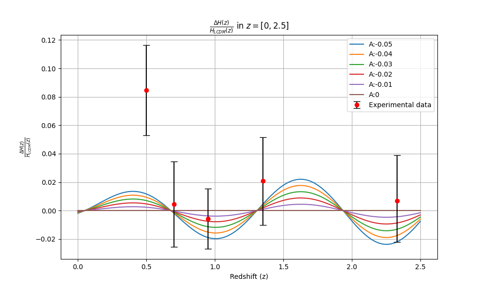
Although the results look promising, our preliminary analysis should not be viewed as conclusive in terms of statistical evidence. With the next data releases the error bars are expected to shrink, and then the data should be able to provide us with a more solid conclusion on the preference of the data for CDM or a dynamical dark energy. The objective of Fig. 1 is to show the range of amplitudes of the oscillating dark energy term which can be in agreement with the DESI constraints. We can see that, for the chosen value , values up to can fit the data within the observational uncertainties. As mentioned earlier, the only data that our model, as well as CDM, does not fit, corresponds to the lowest redshift point, whose validity is still being discussed.
As a preliminary analysis, we performed a test minimizing the of the model with respect to the DESI data, using several different minimization methods and testing several combinations of initial values. The method consists of executing a set of minimization routines, with each minimization sequence having, as initial guesses for the parameters and , the values of a pair that is one of the possible combinations between previously chosen values of and . We chose the initial values of to lie within the range , and those of within . These intervals correspond to initial guesses of suitable parameter values and are starting points for the parameter exploration. In principle one could also vary the phase of the oscillations. However, as mentioned previously, the phase was chosen such that the model is equivalent to the standard model when , which is approximately the beginning of the matter-dominated phase. This is justified by the fact that the oscillatory density of the effective component arising from back-reaction is taken to be proportional to the energy density of matter, and therefore another parametrization should be chosen before the onset of the matter era. We are letting the back-reaction effects build up beginning with the value at . For considerations of late time cosmology this should be fine.
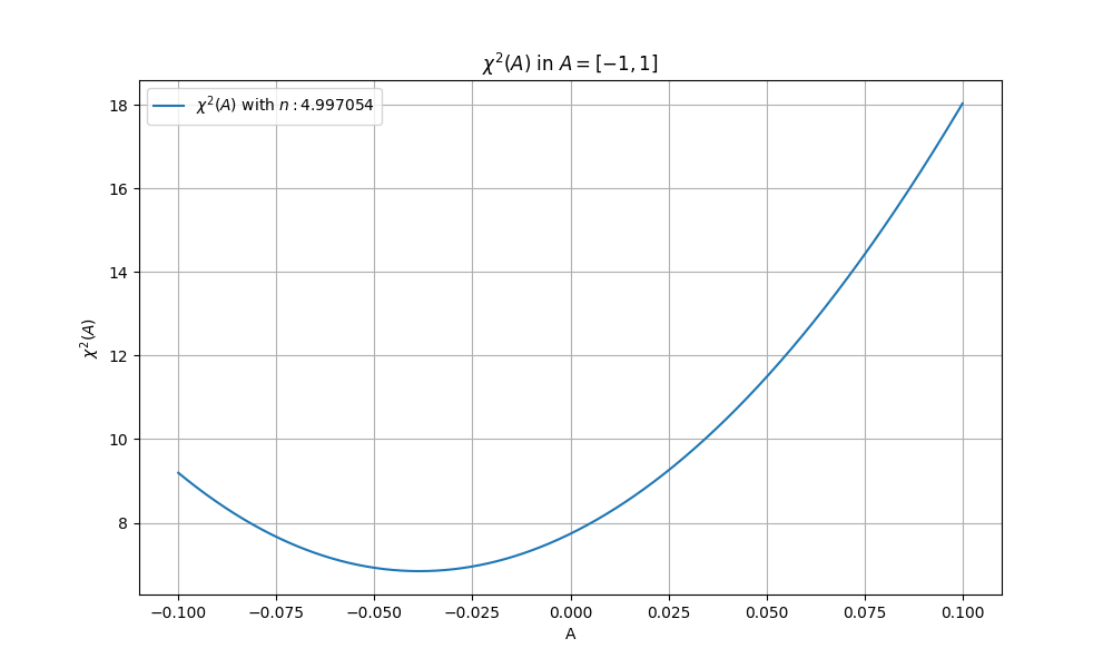
The expression to be minimized is the of (which expresses the relative difference between the proposed model and the standard cosmological model as a function of redshift) with respect to the experimental data from DESI. As described previously, the DESI experimental results were interpreted in terms of , and the error propagation was calculated. Some minimization results lead to a shape more in line with the one indicated by DESI data than others. However, in practically all the cases the obtained from minimizations performed were smaller than the one of the CDM model . On the other hand, this analysis were restricted to amplitudes with order of magnitude or smaller. For large values of the fit is poor. This is shown in Fig.2, where the value of is plotted as a function of the amplitude. The value of chosen for each point in Fig. 2 was the one that provided the best fit for the respective value of the amplitude. From this same Figure we can also see that for higher values of the amplitude the back-reaction model provides a fit worse than the standard model. We can also see from Fig. 2 that the minimum value of the is shifted with respect to the CDM value (which is recovered for the value ). While the error bars still do not allow us to conclude that our model performs better than CDM, these results can be viewed as an indication of the importance of further studies of this model, rather than a firm statistic conclusion.
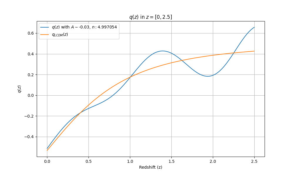
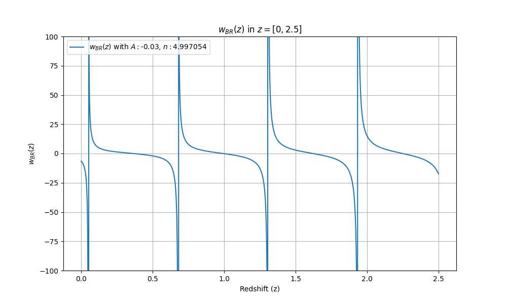
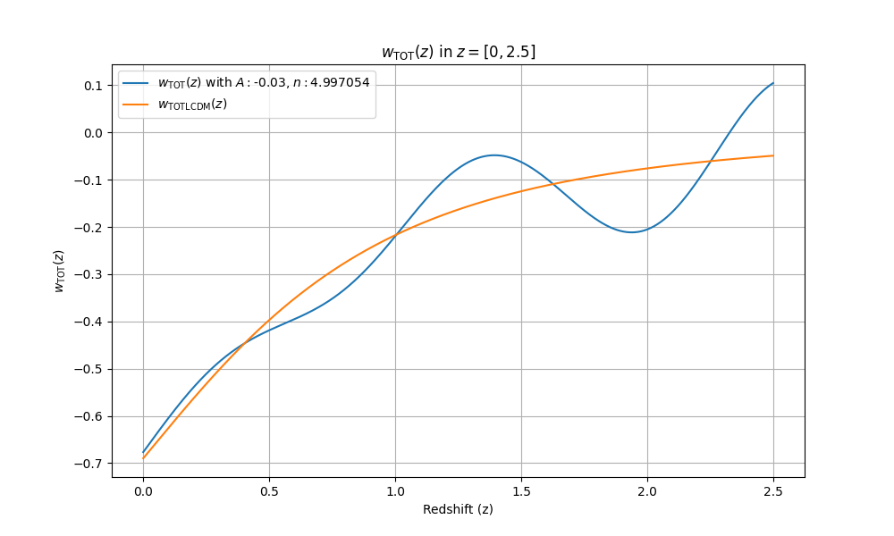
In Figs 3 and 4 we plot, respectively, the deceleration parameter and the equations of state of the back-reaction model and of the total content of the model, according to the equations in Section II. The pair of values was chosen as an illustrative example in all these figures.
In Fig.3 we show the behavior of the deceleration parameter predicted by the back-reaction model for the same values of the parameters and . We can see that this model is able to correctly predict the transition from decelerated to accelerated expansion around the expected redshift.
In Fig.4 (left) we illustrate the evolution of the equation of state for the effective back-reaction fluid, given by Eq.13. We considered again the same values for the parameters and . We can see in the plot at the left that the equation of state shows the average value . One can also see that, at the exact redshifts when crosses zero, a spike can be seen in the plot of . This should be expected from the fluid equation of state . The spikes correspond to the points where the quantity crosses zero in Fig.1. However, this behavior does not correspond to a problem 999A similar behavior can be seen for instance, in the model analyzed in Ref.Tiwari:2024gzo . since the observable quantities in cosmology correspond to integrals of the equation of state over a period of time. Therefore these spikes are not expected to be present in any cosmological observable. In addition, the contribution from the back-reaction effective fluid is always subdominant compared to the other components in the Universe. The effective equation of state of the total fluid has the expected overall behavior, as shown in Fig.4 (right), i.e., it oscillates around the prediction.
Another important aspect to be analyzed is whether the back-reaction model considered here can provide some relief to the Hubble tension, and if so, for which values of the parameters. In order to shed some light to this question we perform an analysis of the value of predicted for different combinations of the parameters and . The analysis uses the method described previously. We show in Fig. 5 a plot of as a function of , , where is the value of chosen from the minimization method performed. As in the previous analysis, we fix our model to be equal to at . We can see in the plot that, for the representative chosen values of the parameters, the predicted by our model is very close to the CDM one. This is partly due to the choice of the fixed A and n and also due to the fact that the back-reaction contribution decreases with , causing the difference with respect to CDM to decrease at later times.
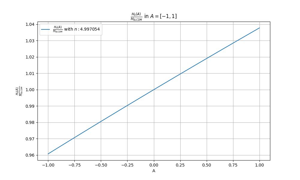
In order to see what could be the highest value of that this model could predict, we can investigate the Hubble constant value for an amplitude as high as . From all the results of our minimizations, the highest value that was obtained was , which is achieved for and . For this same value , but now for a smaller amplitude, , we found values for as high as , which is already more than enough to solve the tension problem. We can see that it can be possible to solve the Hubble tension in our back-reaction model for sufficiently high values of the amplitude. However, from Fig 1 we can see that such high values of does not provide a good fit to DESI data. For the amplitude , which is approximately the highest value that fits DESI error bars for the chosen frequency, we obtain for the Hubble constant of the back-reaction model , i.e., it’s basically indistinguishable from .
It’s important to emphasize again that a priori there is no reason that the amplitude should be independent of time. In fact, from the considerations of back-reaction it is not unreasonable to expect that the effective amplitude of the oscillating contribution to DE performs damped oscillations. In this case, could be large at early times and then slowly decay to a value consistent with the current late time data. This extended scenario might therefore be able to provide a solution of the Hubble tension. On the other hand, without a careful analysis of the fluctuations produced in the model, it is not possible to gauge whether the scenario would be consistent with other constraints, e.g. the value of .
While conclusive results concerning the viability of the model will need to wait for a more complete analysis with the future data, our results shows that the inclusion of back-reaction effects from super-Hubble fluctuations can offer valuable insights in light of recent observational data.
V Conclusion
In the present work, we studied a toy model of oscillating dark energy motivated by considerations of the back-reaction of super-Hubble fluctuations in the late universe. We proposed a parametrization of the oscillating dark energy component to account for the back-reaction effect on the background cosmology (based on the conjectured dynamical scaling fixed point solution describing the back-reaction effect at a fully non-perturbative level). We computed the Hubble parameter at low redshifts predicted by the model, obtaining an oscillatory dynamics. We compared the resulting background cosmology with data from the radial component of the Baryon Acoustic Oscillations obtained from the recent DESI survey Jiang:2024xnu . We found that, for a frequency scale expected from theoretical considerations, a fit to the recent observations can be obtained for a certain range of the amplitude of the oscillation, which is a free parameter in the analysis, and for a frequency of oscillation motivated by the theory. At the present time the observational error bars are still so large that there is no statistically significant advantage of our model over the standard CDM cosmology. But, with upcoming observations the error bars will shrink and may lead to a way to extract a non-vanishing amplitude of an oscillating component to Dark Energy in a reliable way.
We also investigated the impact of our model on the Hubble tension. We found that for a large amplitude of the oscillatory component (such that the energy density in the oscillating term is comparable to the matter energy density) a sufficiently large change in results to explain the Hubble tension. However, if the amplitude is constant in time, such a large value of is inconsistent with the low redshift data. If, on the other hand, depended on time and decreased from a large value near the time of recombination to a small value at the present time, the Hubble constant tension might be successfully adressable. However, detailed studies of the effects of our model on cosmological fluctuations is required to check the consistency of the scenario.
The next step should in fact be to analyze the perturbations in our scenario. This would allow us to make comparisons with other observable quantities, e.g. CMB anisotropies, and in particular the Integrated Sachs Wolf (ISW) effect. In this context, in Ref.Pace:2011kb the behavior of several cosmological observables, such as the linear growth factor, the ISW effect, the number counts of massive structures, and the matter and cosmic shear power spectra were estimated for several oscillating dark energy models. It was shown that, for several of the models considered, then independently of the amplitude and the frequency of the dark energy oscillations, none of these observables showed a significant oscillating behavior as a function of redshift. This is a consequence of the fact that such observables are integrals over functions of the expansion rate along the cosmic history, consequently smoothing oscillatory features below the level of detectability. This analysis was performed under certain assumptions, for instance, supposing that Dark Energy does not cluster on the scales of interest. In addition, the models studied in this reference have a different behavior than the back-reaction model we consider in our work. A complete analysis specific for our scenario is hence still missing, but we believe it might be possible that the main conclusions of the work of Pace:2011kb might also hold for our model. As the observables mentioned are integrals over functions of the expansion rate along the cosmic history, we expect that also in our scenario the oscillatory features will be smoothed, keeping the ISW effect in agreement with current observations.
Another quantity that is going to be investigated in upcoming work is the sound speed predicted in our scenario. Although it may not necessarily be true that the back-reaction model must reproduce the CDM behavior for this quantity, one could expect similar predictions in this regard. Since our model accounts only for the back-reaction of super-Hubble fluctuations, one could expect that a quantity related to the dynamics of sub-Hubble fluctuations, as the sound speed, could follow a similar behavior as the standard model. A further analysis of these aspects will be addressed in a future work.
Our work can be considered to be a first-step analysis limited to the background predictions of the model. Nevertheless, in order to obtain more conclusive results, a study of the predictions of the model for linear perturbations is required. Our results, although preliminary, highlights the importance of considering the back-reaction effect of super-Hubble fluctuations in the late Universe, as such back-reaction effects are expected to be present in any cosmological scenario with entropy fluctuations. We have shown that this provides a dynamics which is interesting in light of recent observational results.
Acknowledgements.
We wish to thank Elisa Ferreira for extensive discussions. M.A.C.A. is supported by Coordenacao de Aperfeicoamento de Pessoal de Nivel Superior (CAPES). L.L.G is supported by research grants from Conselho Nacional de Desenvolvimento Cientıfico e Tecnologico (CNPq), Grant No. 307636/2023-2 and from the Fundacao Carlos Chagas Filho de Amparo a Pesquisa do Estado do Rio de Janeiro (FAPERJ), Grant No. E-26/204.598/2024. RB is supported in part by NSERC and the CRC program.References
- [1] A. M. Polyakov. Infrared instability of the de Sitter space. 9 2012.
- [2] A. M. Polyakov. De Sitter space and eternity. Nucl. Phys. B, 797:199–217, 2008.
- [3] Pawel Mazur and Emil Mottola. Spontaneous Breaking of De Sitter Symmetry by Radiative Effects. Nucl. Phys. B, 278:694–720, 1986.
- [4] E. Mottola. THERMODYNAMIC INSTABILITY OF DE SITTER SPACE. Phys. Rev. D, 33:1616–1621, 1986.
- [5] E. Mottola. Particle Creation in de Sitter Space. Phys. Rev. D, 31:754, 1985.
- [6] N. C. Tsamis and R. P. Woodard. Strong infrared effects in quantum gravity. Annals Phys., 238:1–82, 1995.
- [7] Georges Obied, Hirosi Ooguri, Lev Spodyneiko, and Cumrun Vafa. De Sitter Space and the Swampland. 6 2018.
- [8] Gia Dvali and Cesar Gomez. Quantum Exclusion of Positive Cosmological Constant? Annalen Phys., 528:68–73, 2016.
- [9] Ulf H. Danielsson and Thomas Van Riet. What if string theory has no de Sitter vacua? Int. J. Mod. Phys. D, 27(12):1830007, 2018.
- [10] Keshav Dasgupta, Maxim Emelin, Evan McDonough, and Radu Tatar. Quantum Corrections and the de Sitter Swampland Conjecture. JHEP, 01:145, 2019.
- [11] Alek Bedroya and Cumrun Vafa. Trans-Planckian Censorship and the Swampland. JHEP, 09:123, 2020.
- [12] Alek Bedroya, Robert Brandenberger, Marilena Loverde, and Cumrun Vafa. Trans-Planckian Censorship and Inflationary Cosmology. Phys. Rev. D, 101(10):103502, 2020.
- [13] Robert Brandenberger. Trans-Planckian Censorship Conjecture and Early Universe Cosmology. LHEP, 2021:198, 2021.
- [14] N. C. Tsamis and R. P. Woodard. Relaxing the cosmological constant. Phys. Lett. B, 301:351–357, 1993.
- [15] N. C. Tsamis and R. P. Woodard. Quantum gravity slows inflation. Nucl. Phys. B, 474:235–248, 1996.
- [16] L. Raul W. Abramo, Robert H. Brandenberger, and Viatcheslav F. Mukhanov. The Energy - momentum tensor for cosmological perturbations. Phys. Rev. D, 56:3248–3257, 1997.
- [17] F. Finelli, G. Marozzi, G. P. Vacca, and Giovanni Venturi. Energy momentum tensor of field fluctuations in massive chaotic inflation. Phys. Rev. D, 65:103521, 2002.
- [18] F. Finelli, G. Marozzi, G. P. Vacca, and Giovanni Venturi. Energy momentum tensor of cosmological fluctuations during inflation. Phys. Rev. D, 69:123508, 2004.
- [19] G. Marozzi. Back-reaction of Cosmological Fluctuations during Power-Law Inflation. Phys. Rev. D, 76:043504, 2007.
- [20] Robert H. Brandenberger. Back reaction of cosmological perturbations. In 3rd International Conference on Particle Physics and the Early Universe, pages 198–206, 2000.
- [21] Maqbool Ahmed, Scott Dodelson, Patrick B. Greene, and Rafael Sorkin. Everpresent . Phys. Rev. D, 69:103523, 2004.
- [22] Santanu Das, Arad Nasiri, and Yasaman K. Yazdi. Aspects of Everpresent . Part I. A fluctuating cosmological constant from spacetime discreteness. JCAP, 10:047, 2023.
- [23] Santanu Das, Arad Nasiri, and Yasaman K. Yazdi. Aspects of Everpresent (II): Cosmological Tests of Current Models. 7 2023.
- [24] W. Unruh. Cosmological long wavelength perturbations. 2 1998.
- [25] Ghazal Geshnizjani and Robert Brandenberger. Back reaction and local cosmological expansion rate. Phys. Rev. D, 66:123507, 2002.
- [26] L. R. Abramo and R. P. Woodard. No one loop back reaction in chaotic inflation. Phys. Rev. D, 65:063515, 2002.
- [27] Ghazal Geshnizjani and Robert Brandenberger. Back reaction of perturbations in two scalar field inflationary models. JCAP, 04:006, 2005.
- [28] Giovanni Marozzi, Gian Paolo Vacca, and Robert H. Brandenberger. Cosmological Backreaction for a Test Field Observer in a Chaotic Inflationary Model. JCAP, 02:027, 2013.
- [29] F. Finelli, G. Marozzi, G. P. Vacca, and G. Venturi. Backreaction during inflation: A Physical gauge invariant formulation. Phys. Rev. Lett., 106:121304, 2011.
- [30] M. Gasperini, G. Marozzi, and G. Veneziano. Gauge invariant averages for the cosmological backreaction. JCAP, 03:011, 2009.
- [31] M. Gasperini, G. Marozzi, and G. Veneziano. A Covariant and gauge invariant formulation of the cosmological ’backreaction’. JCAP, 02:009, 2010.
- [32] G. Marozzi. The cosmological backreaction: gauge (in)dependence, observers and scalars. JCAP, 01:012, 2011.
- [33] Giovanni Marozzi and Gian Paolo Vacca. Isotropic Observers and the Inflationary Backreaction Problem. Class. Quant. Grav., 29:115007, 2012.
- [34] L. R. Abramo and R. P. Woodard. Back reaction is for real. Phys. Rev. D, 65:063516, 2002.
- [35] B. Losic and W. G. Unruh. Long-wavelength metric backreactions in slow-roll inflation. Phys. Rev. D, 72:123510, 2005.
- [36] B. Losic and W. G. Unruh. On leading order gravitational backreactions in de Sitter spacetime. Phys. Rev. D, 74:023511, 2006.
- [37] Robert H. Brandenberger and C. S. Lam. Back-reaction of cosmological perturbations in the infinite wavelength approximation. 7 2004.
- [38] Niayesh Afshordi and Robert H. Brandenberger. Super Hubble nonlinear perturbations during inflation. Phys. Rev. D, 63:123505, 2001.
- [39] Vincent Comeau. Perturbative Correction to the Average Expansion Rate of Spacetimes with Perfect Fluids. 4 2023.
- [40] Vincent Comeau and Robert Brandenberger. Back-reaction of long-wavelength cosmological fluctuations as measured by a clock field. Eur. Phys. J. C, 84(3):272, 2024.
- [41] Leonardo Giani, Rodrigo Von Marttens, and Ryan Camilleri. A novel approach to cosmological non-linearities as an effective fluid. 10 2024.
- [42] Robert Brandenberger, Leila L. Graef, Giovanni Marozzi, and Gian Paolo Vacca. Backreaction of super-Hubble cosmological perturbations beyond perturbation theory. Phys. Rev. D, 98(10):103523, 2018.
- [43] A. G. Adame et al. DESI 2024 III: Baryon Acoustic Oscillations from Galaxies and Quasars. 4 2024.
- [44] A. G. Adame et al. DESI 2024 IV: Baryon Acoustic Oscillations from the Lyman Alpha Forest. 4 2024.
- [45] A. G. Adame et al. DESI 2024 VI: Cosmological Constraints from the Measurements of Baryon Acoustic Oscillations. 4 2024.
- [46] R. Calderon et al. DESI 2024: Reconstructing Dark Energy using Crossing Statistics with DESI DR1 BAO data. 5 2024.
- [47] K. Lodha et al. DESI 2024: Constraints on Physics-Focused Aspects of Dark Energy using DESI DR1 BAO Data. 5 2024.
- [48] Guillaume Payeur, Evan McDonough, and Robert Brandenberger. Do Observations Prefer Thawing Quintessence? 11 2024.
- [49] Jun-Qian Jiang, Davide Pedrotti, Simony Santos da Costa, and Sunny Vagnozzi. Non-parametric late-time expansion history reconstruction and implications for the Hubble tension in light of DESI. 8 2024.
- [50] Luis A. Escamilla, Supriya Pan, Eleonora Di Valentino, Andronikos Paliathanasis, José Alberto Vázquez, and Weiqiang Yang. Testing an oscillatory behavior of dark energy. Phys. Rev. D, 111(2):023531, 2025.
- [51] Gong-Bo Zhao et al. Dynamical dark energy in light of the latest observations. Nature Astron., 1(9):627–632, 2017.
- [52] David Tamayo and J. Alberto Vazquez. Fourier-series expansion of the dark-energy equation of state. Mon. Not. Roy. Astron. Soc., 487(1):729–736, 2019.
- [53] C. Rubano, Paolo Scudellaro, E. Piedipalumbo, and S. Capozziello. Oscillating dark energy: A Possible solution to the problem of eternal acceleration. Phys. Rev. D, 68:123501, 2003.
- [54] Eric V. Linder. On oscillating dark energy. Astropart. Phys., 25:167–171, 2006.
- [55] Bo Feng, Mingzhe Li, Yun-Song Piao, and Xinmin Zhang. Oscillating quintom and the recurrent universe. Phys. Lett. B, 634:101–105, 2006.
- [56] Shin’ichi Nojiri and Sergei D. Odintsov. The Oscillating dark energy: Future singularity and coincidence problem. Phys. Lett. B, 637:139–148, 2006.
- [57] Aleksandra Kurek, Orest Hrycyna, and Marek Szydlowski. Constraints on oscillating dark energy models. Phys. Lett. B, 659:14–25, 2008.
- [58] Deepak Jain, Abha Dev, and Jailson Souza Alcaniz. Cosmological bounds on oscillating dark energy models. Phys. Lett. B, 656:15–18, 2007.
- [59] Diego Saez-Gomez. Oscillating Universe from inhomogeneous EoS and coupled dark energy. Grav. Cosmol., 15:134–140, 2009.
- [60] Aleksandra Kurek, Orest Hrycyna, and Marek Szydlowski. From model dynamics to oscillating dark energy parametrisation. Phys. Lett. B, 690:337–345, 2010.
- [61] F. Pace, C. Fedeli, L. Moscardini, and M. Bartelmann. Structure formation in cosmologies with oscillating dark energy. Mon. Not. Roy. Astron. Soc., 422:1186–1202, 2012.
- [62] Supriya Pan, Emmanuel N. Saridakis, and Weiqiang Yang. Observational Constraints on Oscillating Dark-Energy Parametrizations. Phys. Rev. D, 98(6):063510, 2018.
- [63] Grigoris Panotopoulos and Ángel Rincón. Growth index and statefinder diagnostic of Oscillating Dark Energy. Phys. Rev. D, 97(10):103509, 2018.
- [64] Mehdi Rezaei. Observational constraints on the oscillating dark energy cosmologies. Mon. Not. Roy. Astron. Soc., 485:550, 2019.
- [65] Tian-Ying Yao, Rui-Yun Guo, and Xin-Yue Zhao. Constraining neutrino mass in dynamical dark energy cosmologies with the logarithm parametrization and the oscillating parametrization. 11 2022.
- [66] Mehdi Rezaei. Oscillating Dark Energy in Light of the Latest Observations and Its Impact on the Hubble Tension. Astrophys. J., 967(1):2, 2024.
- [67] S. X. Tián. Cosmological consequences of a scalar field with oscillating equation of state: A possible solution to the fine-tuning and coincidence problems. Phys. Rev. D, 101(6):063531, 2020.
- [68] Shahnawaz A. Adil, Özgür Akarsu, Eleonora Di Valentino, Rafael C. Nunes, Emre Özülker, Anjan A. Sen, and Enrico Specogna. Omnipotent dark energy: A phenomenological answer to the Hubble tension. Phys. Rev. D, 109(2):023527, 2024.
- [69] Manasse R. Mbonye. Is cosmic dynamics self-regulating? Int. J. Mod. Phys. D, 32(12):2350076, 2023.
- [70] Manasse R. Mbonye. The Big Bang: Origins and initial conditions from Self-Regulating Cosmology (SRC) model. 4 2024.
- [71] Gong-Bo Zhao, Jun-Qing Xia, Mingzhe Li, Bo Feng, and Xinmin Zhang. Perturbations of the quintom models of dark energy and the effects on observations. Phys. Rev. D, 72:123515, 2005.
- [72] Viatcheslav F. Mukhanov, H. A. Feldman, and Robert H. Brandenberger. Theory of cosmological perturbations. Part 1. Classical perturbations. Part 2. Quantum theory of perturbations. Part 3. Extensions. Phys. Rept., 215:203–333, 1992.
- [73] Viatcheslav F. Mukhanov, L. Raul W. Abramo, and Robert H. Brandenberger. On the Back reaction problem for gravitational perturbations. Phys. Rev. Lett., 78:1624–1627, 1997.
- [74] Robert H. Brandenberger. Back reaction of cosmological perturbations and the cosmological constant problem. In 18th IAP Colloquium on the Nature of Dark Energy: Observational and Theoretical Results on the Accelerating Universe, 10 2002.
- [75] L. Raul W. Abramo. The Back reaction of gravitational perturbations and applications in cosmology. Other thesis, 9 1997.
- [76] David H. Weinberg, Michael J. Mortonson, Daniel J. Eisenstein, Christopher Hirata, Adam G. Riess, and Eduardo Rozo. Observational Probes of Cosmic Acceleration. Phys. Rept., 530:87–255, 2013.
- [77] Shi-Fan Chen et al. Baryon Acoustic Oscillation Theory and Modelling Systematics for the DESI 2024 results. 2 2024.
- [78] Timothy Clifton and Neil Hyatt. A radical solution to the Hubble tension problem. JCAP, 08:052, 2024.
- [79] Yashi Tiwari, Ujjwal Upadhyay, and Rajeev Kumar Jain. Exploring cosmological imprints of phantom crossing with dynamical dark energy in Horndeski gravity. 12 2024.