Fast control allocation algorithm for tilt-rotor VTOL aircraft

Abstract

Control algorithms initially developed for tilt-wing vertical take-off and landing (VTOL) aircraft are adapted to the tilt-rotor design. The main difference between the two types of planes is the more complicated interaction between propellers and wings in the tilt-rotor design. Unlike tilt-wing design, the tilt-rotor case varies the angle between the propeller disk and wing cord line, thus introducing a non-linear dependency of lift on thrust and tilt angle. In this paper we develop a precise control allocation method, utilizing Groebner basis algorithms to mask the non-linearity of the control action and allow the use of linear time-invariant control laws for attitude and velocity control architectures. The performance of our approach is discussed and quantified w.r.t. the accuracy of the developed propeller-wing interaction model.

1 Introduction

The aerospace industry has been disrupted in recent years with the introduction of electric vertical take-off and landing (VTOL) aircraft. These prototypes are quite diverse at the current stage of development, with various configurations well described in [10]. All recent designs utilize multiple, electrically powered propellers that achieve thrust vectoring by either tilting the propellers (tilt-rotor), the entire wing (tilt-wing), or the entire aircraft (tail-sitter). Arguably, the best-researched type is the tilt-wing, utilizing a tiltable main wing with distributed propulsion fixed to the wing structure (see [9], [15] and [1]). The propellers interact with the wing, coupling thrust with local lift generation. The thrust and lift coupling phenomena was investigated for traditional distributed propulsion [14] and for tilt-wing configuration [8] cases. For these configurations, both high-fidelity computational fluid dynamics (CFD) models as well as control designed oriented reduced complexity models have been developed, see [14].

The control of such an over-actuated design is challenging. The control architecture significantly deviates from the traditional aircraft control scheme, introducing more advanced control allocation algorithms with daisy chain protocols for actuator selection [9] and state-dependent gain scheduling feedback control. The nonlinearity of the longitudinal dynamics justified the utilization of non-linear model predictive [15] and feedback linearization [1] algorithms for airspeed and altitude control. It should be noted that such algorithms are not typically used in the aerospace industry as their stability and performance analysis is more challenging than in the case of traditional linear time invariant (LTI) control laws.

Our work adapts the previously described algorithms to the tilt-rotor type of VTOL aircraft. The design utilizes distributed propeller propulsion with vertical thrust vectoring, as shown in Figure 1.

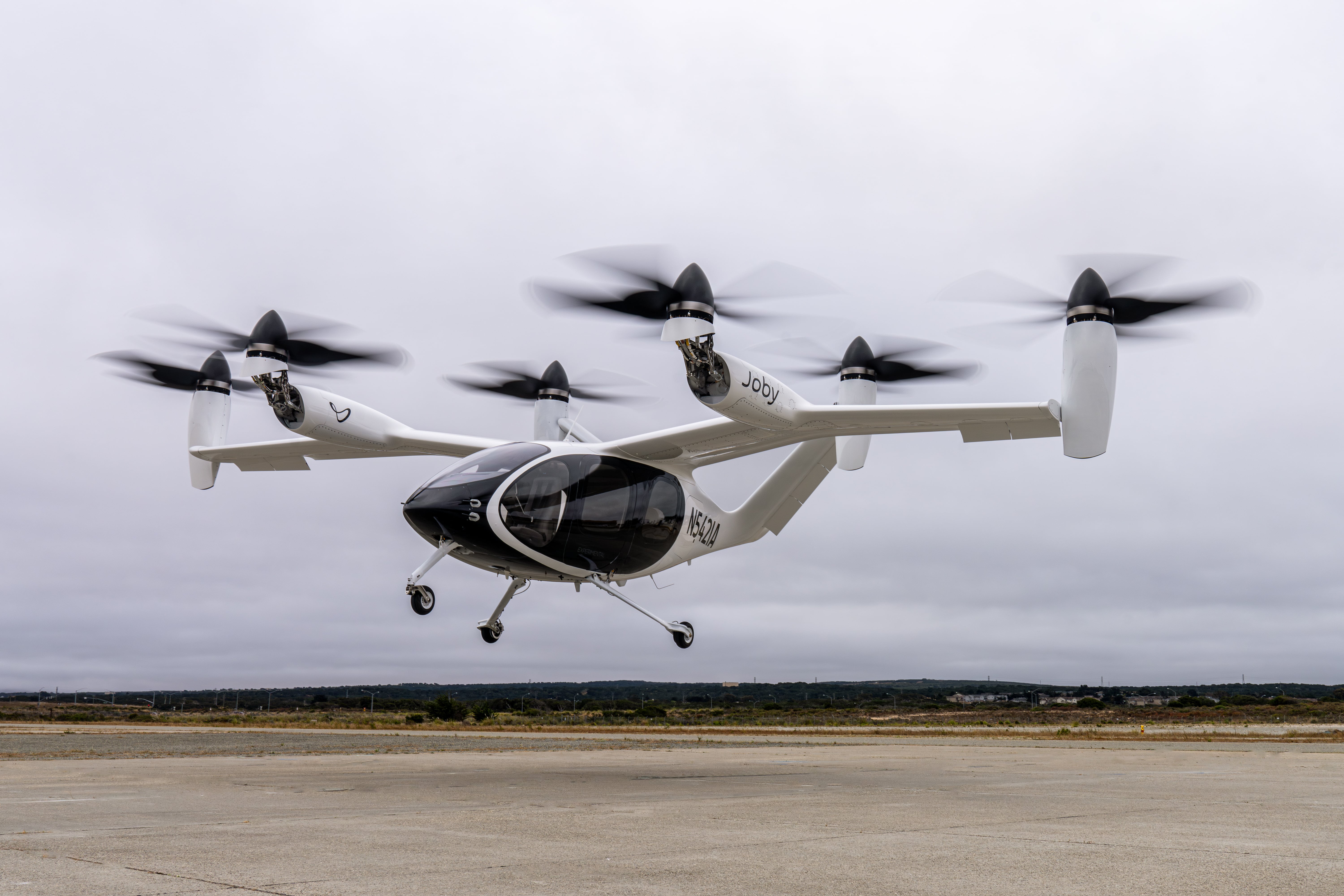
(a) hover configuration

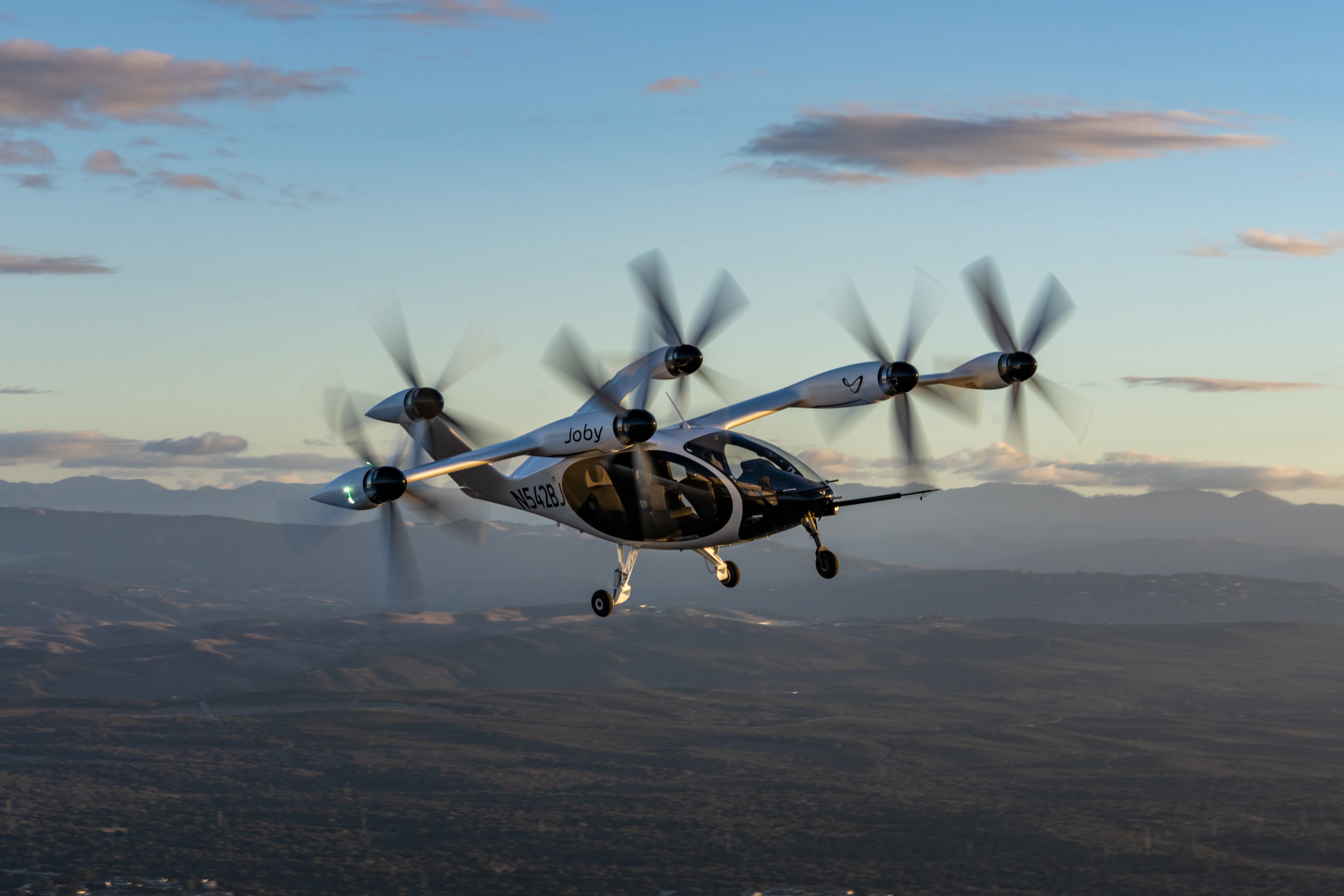
(b) flight configuration

Figure 1: Joby aviation tilt-rotor pre-production aircraft, shown in hover (left) and cruise (right) configuration. Reproduced from www.jobyaviation.com

Unlike tilt-wing design, the tilt-rotor propellers are not in fixed position w.r.t. the wing. This design feature increases the complexity of coupling between thrust and lift, as described in [10]. The propeller downwash changes the local angle of attack according to the propeller tilt angle and generated thrust. In high-tilt angle configurations, the downwash misses the wing completely, creating a decoupled system. An accurate control allocation of the propeller-wing actuator system has not been developed so far.

Our goal is to propose a control allocation method that transforms the inputs of the controlled system from physical actuators into forces acting at each actuator location. We consider physical actuators to be thrust values and tilt angles of individual propellers, together with the control surface deflections. Such transformation would mask the system’s nonlinearities and would enable a direct command of the forces and moments acting on the system. In this paper, we propose and analyze the corresponding control laws and develop the underlying simplified design models.

The propeller-wing interaction for the tilt-rotor case is considerably more complex compared to the tilt-wing case. Therefore, we need to expand the established tilt-wing mathematical models to describe the tiltable propeller interaction with the wing. As in the case of tilt-wing design [9], we model the interaction between free-stream and the induced airflow as a linear combination of two independent vector fields. The aerodynamic analysis in [14] shows that the propeller-disk approach tends to overestimate the resulting induced airflow’s influence on lift. To compensate for this discrepancy, we introduce an additional coefficient to modulate the calculated airflow and thus control the ratio between thrust and lift. The resulting model inputs are thrust and tilt angle commands respectively and its outputs are generated forces in the body coordinate frame, parametrized by airspeed, air density, and angle of attack.

The developed mathematical model is then inverted for the control allocation purposes. The model inversion calculates the actuator commands based on the required forces of the propeller-wing component. The highly non-linear relation between the thrust vector and lift/drag values prevents us from describing the inversion as a simple rational function. Instead, we develop Groebner basis algorithms to find a precise solution, dependent on the required forces and aircraft state coefficients. To determine the values of actuator configurations, we find the eigenvalues of related multiplication matrices corresponding to the actuator commands. Resulting eigenvalue algorithms implemented in Matlab can be effectively evaluated within milliseconds. This computation speed enables the deployment of the algorithm in a real-time control scheme.

The described approach is accurate in situations with small tilt angles, corresponding to cruise and high-speed transition phases of flight. An additional, straightforward, algorithm is used to allocate control for high tilt-angles where the propeller and wing are decoupled, corresponding to hovering and slow-speed transition phases. A linear combination of control action is proposed to achieve smooth transition from coupled to decoupled regions, expected during transition between hover and cruise. The resulting design achieves accurate control allocation throughout the entire flight envelope and enables the usage of single LTI control laws for attitude and airspeed control, as described in our previous work [3].

We utilize the control allocation approach to quantify the achievable performance and stability of feedback control w.r.t. the aircraft parameters and the accuracy of propeller-wing interaction model. This analysis exploits the fact that the resulting system behaves from a control perspective as a set of double integrators. We develop and present relations between model accuracy and achievable performance.

To summarize, our main goal is to propose a novel approach to the tilt-rotor controller design, that can utilize simple feedback laws and solve the system’s nonlinearities, caused by the propeller-wing interaction, in the control allocation algorithms that can be easily analyzed and implemented. The advantage of our approach when compared to previous work done in tilt-rotor control [19, 2, 1] is a more accurate control allocation due to the inclusion of the propeller-wing interaction. The improved accuracy in control allocation is expected to improve LTI feedback control, with more consistent performance throughout the flight envelope.

The paper is divided into the following sections. In section 2 we describe the control achitecture for tilt-rotors that motivates the control allocation problem solved in this paper. Following that, the section 3 describes the mathematical model of propeller and wing interaction for which we define the control allocation. The model-based control allocation is then described in section 4, with accuracy and computational speed testing included in this section. Finally we conclude the paper in section 5.

2 Control system architecture

In this section, we describe our overall approach to the tilt-rotor aircraft control, and we highlight the specific contribution of this paper to the control architecture illustrated in Figure 2.

Our research aims to create a unified architecture that regulates all aircraft states through feedback designs resembling current flight control algorithms. To achieve this goal, we develop advanced control allocation methods in this paper, which can be combined with dynamics inversion procedures previously developed in [3]. This approach aims to compensate for the variance and non-linearity of the aircraft’s natural dynamics. The process is based on the exact-linearization approach in non-linear control theory and was previously utilized in [9].

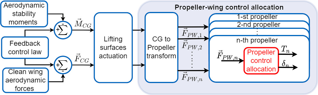
Figure 2: Schematic description of control architecture.

Our contribution to the feedback controller design is the description of the model-based control allocation method for propeller-wing interaction, accompanied by a corresponding analysis of the modeling uncertainty’s effect on the controller performance.

The inputs of the control allocation system are the moments $\vec{M}_{r}$ and forces $\vec{F}_{r}$ requested by the feedback controller, combined with the aerodynamic forces generated by the clean wing sections.

Initially, the control allocation uses the control surfaces deflection to generate the required moments $\vec{M}_{r}$ on the system. We assume that the aerodynamic surfaces deflections $\delta_{A}$, $\delta_{E}$ and $\delta_{R}$ are fully decoupled with the control allocation being expressed as

$$\begin{pmatrix}\delta_{A}\\ \delta_{E}\\ \delta_{R}\end{pmatrix}={\underbrace{\begin{pmatrix}C_{l}^{A}(q)&0&0\\ 0&C_{m}^{E}(q)&0\\ 0&0&C_{n}^{R}(q)\end{pmatrix}}_{C_{A}}}^{-1}\vec{M}_{r},$$ (1)

where $C_{l}^{A}(q)$, $C_{m}^{E}(q)$ and $C_{n}^{R}(q)$ are the aerodynamic control derivatives, relating aerodynamic surface deflections and corresponding moments generated at center of gravity (CG). The allocation uncertainty caused by the model $\begin{bmatrix}M(\delta_{A},\delta_{E},\delta_{R})&F(\delta_{A},\delta_{E},\delta_{R})\end{bmatrix}^{T}$ inaccuracy is described with coefficients $\epsilon_{0,A}$, representing constant offset of generated forces and $\epsilon_{1,A}$, representing the relative error of the modeled slope

$$\vec{u}_{a}=\vec{\epsilon}_{0,A}+C_{A}\cdot\epsilon_{1,A}\cdot C_{A}^{-1}\cdot\vec{M}_{r}.$$ (2)

In order to prevent the jittering movement of aerodynamic surfaces in lower speed conditions, we only allocate a fraction $\phi(q)$ of the required moment with the aerodynamic surfaces. The airspeed-dependent aerodynamic surfaces actuation is described in our previous work [3]. The calculated deflection is used to estimate the additional forces generated by the change in lift and drag through the change of local aerodynamic coefficients $C_{L}$ and $C_{D}$ due to the deflection of the control surface. We describe this effect in equations (15), (17) and (19).

The remaining forces and moments are generated using the tiltable propeller actuation. To define the transformation from action at CG to propeller-centered forces, we describe the transformation from the $i$th propeller-wing forces vector $\vec{F}_{i}=\begin{bmatrix}F_{x}&&F_{z}\end{bmatrix}^{T}$ through the distance vector $\vec{L}_{i}$ between the CG and propeller-wing actuated point as

$$\begin{bmatrix}\vec{M}_{CG}^{i}\\ \vec{F}_{CG}^{i}\end{bmatrix}=\begin{bmatrix}M_{x}^{i}\\ M_{y}^{i}\\ M_{z}^{i}\\ F_{x}^{i}\\ F_{z}^{i}\end{bmatrix}=\begin{bmatrix}0&L_{y}^{i}\\ L_{z}^{i}&L_{x}^{i}\\ L_{y}^{i}&0\\ 1&0\\ 0&1\end{bmatrix}\cdot\begin{bmatrix}F_{x}\\ F_{z}\end{bmatrix}=L_{i}\cdot\vec{F}_{i}.$$ (3)

To combine $n$ propellers, their influences are added together

$$\begin{bmatrix}\vec{M}_{CG}\\ \vec{F}_{CG}\end{bmatrix}=\sum_{i}\begin{bmatrix}\vec{M}_{CG}^{i}\\ \vec{F}_{CG}^{i}\end{bmatrix}=\begin{bmatrix}L_{1}&\cdots&L_{n}\end{bmatrix}\cdot\begin{bmatrix}\vec{F}_{1}\\ \vdots\\ \vec{F}_{n}\end{bmatrix}=L\cdot\vec{F}.$$ (4)

Using pseudo-inversion of the distance matrix $L$, the torque and force commands are transformed into required forces for individual propellers $\vec{F}=L^{+}\cdot\begin{bmatrix}\vec{M}_{CG}&\vec{F}_{CG}\end{bmatrix}^{T}$.
We assume that the control allocation uncertainty can be described in the same manner as in the allocation of aerodynamic surfaces case with constant uncertainty value $\vec{\epsilon}_{0,p}$ and gain uncertainty $\epsilon_{1,p}$ combined into an affine function

$$\vec{u}_{p}=\vec{\epsilon}_{0,p}+L\cdot\epsilon_{1,p}\cdot L^{+}\cdot\begin{bmatrix}\vec{M}_{CG}^{i}\\ \vec{F}_{CG}^{i}\end{bmatrix}.$$ (5)

Actuation saturation and fault-tolerance issues are solved by the daisy chain method [5]. As the set of equations is under-determined, the pseudo-inverse approach minimizes the Euclidean norm of output vector $\vec{F}$ [16]. This property can be utilized to equalize the load on individual propellers by normalizing the $\vec{F}$ values with the maximal achievable thrust $\vec{F}_{max}$.

The control uncertainty of the complete control allocation with $\phi(q)$ and $\psi=(1-\phi)$ fraction allocated with aerodynamic surfaces is expressed as an affine mapping of the reference forces

$$\begin{split}\vec{u}&=\begin{bmatrix}\phi&\psi\end{bmatrix}\cdot\begin{bmatrix}\vec{\epsilon}_{0,a}\\ \vec{\epsilon}_{0,p}\end{bmatrix}+(I+\begin{bmatrix}\phi&\psi\end{bmatrix}\cdot\begin{bmatrix}C\epsilon_{1,a}C^{-1}\\ L\epsilon_{1,p}L^{+}\end{bmatrix})\cdot\vec{u}_{r}\\ &=\vec{\epsilon}_{0}+(1+\epsilon_{1})\cdot\vec{u}_{r},\end{split}$$ (6)

where the $\epsilon_{1}$ matrix consists of uncertainties in forces and moments generated by aerodynamic surfaces and propellers combined. The system is considered decoupled only if matrix $A=I+\epsilon_{1}$ is diagonally dominant, meaning

$$|a_{ii}|\geq\sum_{j\neq i}|a_{ij}|\quad\forall i.$$ (7)

If this condition is achieved throughout the aircraft flight envelope, the system control can be designed for multiple independent single-input single-output (SISO) loops. However, it should be noted that when the values $|a_{ii}|$ and $\sum_{j\neq i}|a_{ij}|$ are comparable, then the system will exhibit some coupling behavior.

The last and arguably most difficult step is an accurate transformation from the required forces at the propeller-wing level $\vec{F}_{i}$ to the thrust $T_{i}$ and tilt angle $\delta_{i}$ commands, reflecting the manipulated variables of the aircraft. This step is highlighted in red in Figure 2. This accurate control allocation is our main contribution. It will be described in the remainder of the paper, starting with the description of the corresponding mathematical model and followed by the development of the control allocation algorithm.

Description of control allocation problem

The problem can be described as inverting the forward map $\mathbb{R}^{2}\to\mathbb{R}^{2}$ from the thrust $T$ and tilt angle $\delta$ values (called inputs) to forces $F_{x}$, $F_{z}$ (called outputs) for varying system variables (called parameters), namely airspeed $v_{\infty}$, air density $\rho$, angle of attack $\alpha_{\infty}$ and the coefficient of lift $cl_{0}$. The trigonometric expresion of the forward map is developed in section 3.

3 Trigonometric forward map expression

The propeller-wing interaction model represents the interaction between propeller thrust and aerodynamic forces created by the corresponding wing section. The system geometry is shown in Figure 3.

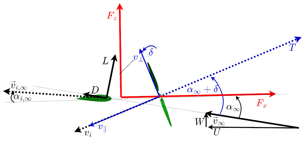
Figure 3: Geometry of the propeller wing configuration, with propeller and wing components (green), propeller-related vectors (blue), overall forces (red), and wind-related vectors (black).

3.1 Propeller disk model

The propeller model is based on the widely used actuator disk theory [18]. The rotor is modeled as an infinitely thin disk, inducing kinetic energy to the air stream as a reaction to a provided thrust.

The propeller disk is affected by the airstream, described by a constant velocity vector $\vec{v}_{\infty}=\begin{bmatrix}U&V&W\end{bmatrix}$, and corresponding angle of attack

$$\alpha_{\infty} =\arctan{\frac{W}{U}}.$$ (8)

The propeller generates thrust vector $\vec{T}$, perpendicular to the disk surface, and induces stream velocity vector $\vec{v}_{i}^{\infty}$. We divide the $\vec{v}_{\infty}$ flow into a component parallel to the thrust vector

$$v_{\parallel}=||\vec{v}_{\infty}||\cdot\cos(\alpha_{\infty}+\delta),$$ (9)

and the remaining perpendicular component

$$v_{\perp}=\sqrt{||\vec{v}_{\infty}||^{2}-v_{\parallel}^{2}}=||\vec{v}_{\infty}||\cdot\sin(\alpha_{\infty}+\delta).$$ (10)

The propeller thrust depends on the propeller speed $\omega$ through the well-known relation [11]

$$T=c_{T}\cdot\rho\cdot\omega^{2}\cdot D^{4},$$ (11)

where $\rho$ is the air density, $D$ is the propeller diameter and $c_{T}$ is the thrust coefficient. We assume that a lower level algorithm controls the thrust and can be used as model input.

As the propeller acts on the air to generate the required thrust, it accelerates the component of airflow, parallel to the thrust vector into

$$v_{i}=\sqrt{\frac{2\cdot T}{\eta_{p}\cdot\rho\cdot A_{p}}+v_{\parallel}^{2}},$$ (12)

where $\eta_{p}$ is the propeller efficiency factor. It should be noted that the stream velocity $v_{i}$ is achieved at a substantial distance behind the propeller surface. At the propeller disk, the airspeed $v_{i,p}$ equals the average of $v_{i}$ and $v_{\parallel}$. If we neglect air viscosity, the airstream accelerates to an infinite distance, reaching a magnitude

$$||\vec{v}_{i,\infty}||=\sqrt{v_{i}^{2}+v_{\perp}^{2}}$$ (13)

with the angle of attack with respect to the thrust vector

$$\alpha_{i}=\arctan(\frac{v_{\perp}}{v_{i}})-\delta=\arctan(\frac{v_{\perp}\cdot\cos(\delta)-v_{i}\cdot\sin(\delta)}{v_{\perp}\cdot\sin(\delta)+v_{i}\cdot\cos(\delta)})$$ (14)

being decreased for $T>0$. The described relations should hold for the airstream at any distance from the propeller by changing $v_{i}$ with the local induced velocity. We will refer to the airspeed and angle of attack values over the wing as $v_{i}$ and $\alpha_{i}$, respectively.

3.2 Clean wing

The aerodynamics of the free wing, as described in Figure 3, is well described in [17]. The air-stream flowing over the wing $\vec{v}_{w}$ generates a lift

$$L=\frac{1}{2}\rho\cdot A_{w}\cdot C_{L}\cdot||\vec{v}_{w}||^{2},$$ (15)

where $A_{w}$ is the wing area, and $C_{L}$ is the coefficient of lift, typically described as an affine function of the angle of attack $\alpha_{w}$ given by

$$C_{L}=c_{L0}+c_{L\alpha}\cdot\alpha_{w},$$ (16)

located at the wing center of pressure. It should be noted that the component of airflow parallel to the wing cord does not affect the generated aerodynamic forces. As a secondary effect, the wing creates an aerodynamic drag

$$D=\frac{1}{2}\rho\cdot A_{w}\cdot C_{D}\cdot||\vec{v}_{w}||^{2},$$ (17)

where the coefficient of drag $C_{D}$ is an affine function of $\alpha_{w}^{2}$ given by

$$C_{D}=c_{D0}+c_{D\alpha}\cdot\alpha_{w}^{2}.$$ (18)

This description neglects the effect of flow separations at high angles of attack (stall). The simplification is typically not problematic for commercial aircrafts, where high-$\alpha$ maneuvers are not expected.

Control surface deflection $\delta_{s}$ modifies the $c_{L}$ and $c_{D}$ coefficients according to

$$C_{L}^{s} =C_{L}+c_{L}^{\delta_{s}}\cdot\delta_{s}, C_{D}^{s} =C_{D}+c_{D}^{\delta_{s}}\cdot\delta_{s}.$$ (19)

This simplification is based on [12]. Note that the lift and drag forces are defined in the stability frame (aligned with the airstream vector). To align the forces with the wing coordinate system, the following rotation by $\alpha_{w}$ should be used:

$$\vec{F}_{w}=\begin{bmatrix}F_{x,w}\\ F_{z,w}\end{bmatrix}=\begin{bmatrix}\cos(\alpha_{w})&-\sin(\alpha_{w})\\ \sin(\alpha_{w})&\cos(\alpha_{w})\end{bmatrix}\cdot\begin{bmatrix}L\\ D\end{bmatrix}.$$ (20)

3.3 Interaction between propeller and wing

Trigonometric forward map expression

The developed model for propeller-wing interaction resulted in a $\mathbb{R}^{2}\to\mathbb{R}^{2}$ forward map from propeller thrust $T$ and tilt angle $\delta$ (inputs) to generated forces $F_{x}$, $F_{z}$ (outputs) of the propeller and wing. The model parameters are $v_{\infty}$, $\rho$, $\alpha_{\infty}$ and $cl_{0}$. The model can be described as $$\begin{bmatrix}F_{x}\\ F_{z}\end{bmatrix}=\begin{bmatrix}T\cdot\cos(\delta)+\frac{1}{2}\cdot(cl_{0}+cl_{\alpha}\cdot\alpha_{w})\cdot\rho\cdot(v_{\infty}^{2}+\frac{2\cdot T}{\eta_{p}\cdot\rho\cdot A_{p}})\cdot A_{w}\\ T\cdot\sin(\delta)-\frac{1}{2}\cdot(cd_{0}+cd_{\alpha}\cdot\alpha_{w}^{2})\cdot\rho\cdot(v_{\infty}^{2}+\frac{2\cdot T}{\eta_{p}\cdot\rho\cdot A_{p}})\cdot A_{w}\\ \end{bmatrix},$$ (21) with $$\alpha_{w}=\arctan(\frac{cos(\delta)\cdot sin(\alpha_{\infty}+\delta)-sin(\delta)\cdot(\sqrt{\frac{2\cdot T}{\eta_{p}\cdot\rho\cdot A_{p}})+v_{\infty}\cdot cos(\alpha_{\infty}+\delta)})\cdot v_{\infty}^{-1}}{cos(\delta)\cdot(\sqrt{\frac{2\cdot T}{\eta_{p}\cdot\rho\cdot A_{p}})+v_{\infty}\cdot cos(\alpha_{\infty}+\delta)})\cdot v_{\infty}^{-1}+sin(\delta)\cdot sin(\alpha_{\infty}+\delta)}),$$ (22) where $A_{w}$, $A_{p}$, $cl_{\alpha}$, $cd_{\alpha}$, $cd_{0}$ are given constants. The model heavily depends on trigonometric functions. Its analytical inversion for the control allocation purposes is therefore a nontrivial problem. As demonstrated in Figure 5, the model map has a singularity for zero thrust $T$ and is, therefore, badly conditioned in the region of low thrust. This feature of the system prevents a robust usage of gradient search algorithms to solve the model inversion. The solution of the inversion is the topic of section 4.

With separate models of propeller and wing, the interaction between these two systems needs to be defined. Only the influence of the propeller on the wing is considered in this paper. The influence of the wing on the propeller, reflected in its efficiency reduction, is not considered. The induced velocity $v_{i}$ in the wing location, called $v_{i,w}$, depends on the distance from the propeller disk and can be expressed as the weighted average of $v_{i}$ and $v_{\parallel}$

$$v_{i,w}=f_{w}\cdot v_{i}+(1-f_{w})\cdot v_{\parallel}.$$ (23)

The $f_{w}$ value will be used as an optimization parameter. It should be noted that the propeller’s induced air stream does not always interact with the wing. The geometry of the propeller and wing is shown in Figure 4.

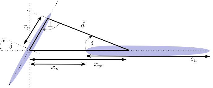
Figure 4: Geometry of the interaction between propeller-induced airflow and wing location.

Assuming non-viscous air, the induced flow only affects the area behind the propeller disk, as is shown in [7]. As the tilt-angle $\delta$ increases, the intersection of $\vec{d}$ and the wing cord line moves closer to the wing’s leading edge (LE). The distance from the propeller center to the LE equals $x_{p}$. The distance from the $\vec{d}$ and cord line intersection to the propeller center is equal to $x_{w}=\frac{r_{p}}{\cos(\delta)},$ where $r_{p}$ corresponds to the local radius of the propelled air stream. Due to conservation of airflow, the area of the induced flow reduces as the airflow increases. The ratio between the propeller and the local radius can be expressed as

$$r_{p}=r_{p}\cdot\sqrt{\frac{v_{i,p}}{v_{i,w}}}.$$ (24)

If the wing is located behind the propeller, then $v_{i,p}<v_{i,w}$, resulting in a reduction of local flow radius up to a ratio of $\frac{1}{\sqrt{2}}$ at $v_{i,p}$ equal to $v_{i}$. The description assumes two edge cases:

• $x_{w}>x_{p}+c_{w}$: the induced airflow encompasses the entire wing;

• $x_{w}<x_{p}$: the airflow over the wing is equal to free-stream.

In the remaining cases, we assume that the flow combines free-stream and induced airflow, as described in the following formula:

$$v_{i,w}=\frac{d_{w}}{x_{w}-x_{p}}\cdot(f_{w}\cdot v_{i}+(1-f_{w})\cdot v_{\parallel})+(1-\frac{d_{w}}{x_{w}-x_{p}})\cdot v_{\parallel}.$$ (25)

Finally, the overall force vector that combines aerodynamic forces with the thrust projections is defined as

$$\vec{F}=\begin{bmatrix}F_{x}\\ F_{z}\end{bmatrix}=\vec{F}_{w}+\begin{bmatrix}\cos{\delta}\cdot T\\ \sin{\delta}\cdot T\end{bmatrix},$$ (26)

where $\vec{F}_{w}$ is described in (20), $T$ is the propeller thrust and $\delta$ its tilt-angle.

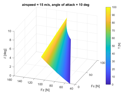
(a) hover configuration

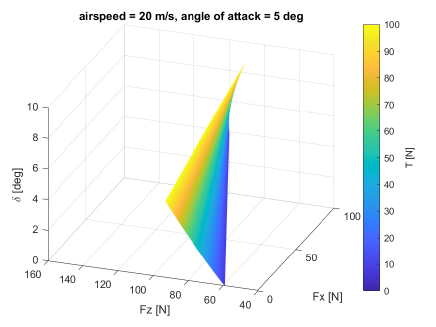
(b) flight configuration

Figure 5: Two examples of modeled relation between model inputs (thrust $T$ and tilt angle $\delta$ and model outputs ($F_{x}$ and $F_{z}$) with varying parameter values ($v_{\infty}$ and $\alpha_{\infty}$)

4 Control allocation algorithm

Polynomial reformulation of the forward map

Under assumptions 1 and 2, using lifting variables $s$, $c$, $v_{w}$, and $\alpha_{w}$ we reformulate the forward map as a system of polynomial equations: $$F_{x}=T\cdot(c\cdot\cos(\alpha_{\infty})+s\cdot\sin(\alpha_{\infty}))+\frac{1}{2}\cdot(cl_{0}+cl_{\alpha}\cdot\alpha_{w})\cdot\rho\cdot(v_{\infty}^{2}+\frac{2\cdot T}{\eta_{p}\cdot\rho\cdot A_{p}})\cdot A_{w}$$ (27) $$F_{z}=T\cdot(s\cdot\cos(\alpha_{\infty})+c\cdot\sin(\alpha_{\infty}))-\frac{1}{2}\cdot(cd_{0}+cd_{\alpha}\cdot\alpha_{w}^{2})\cdot\rho\cdot(v_{\infty}^{2}+\frac{2\cdot T}{\eta_{p}\cdot\rho\cdot A_{p}})\cdot A_{w}$$ (28) $$\alpha_{w}\cdot(c\cdot v_{w}+s\cdot(s\cdot\cos(\alpha_{\infty})+c\cdot\sin(\alpha_{\infty})))=(c\cdot(s\cdot\cos(\alpha_{\infty})+c\cdot\sin(\alpha_{\infty}))+s\cdot v_{w}$$ (29) $$v_{w}^{2}=(v_{\infty}\cdot(c\cdot\cos(\alpha_{\infty})+s\cdot\sin(\alpha_{\infty}))^{2}+\frac{2\cdot T}{\eta_{p}\cdot\rho\cdot A_{p}})$$ (30) $$s^{2}+c^{2}=1.$$ (31) This reformulation allow us to use the Groebner bases techniques. Given the required forward model outputs and its parameters we compute the corresponding inputs and lifting variables. The propeller thrust $T$ is obtained directly, while the tilt angle can be found through the $\delta=asin(s)$ relation.

To develop the control allocation algorithm, we need to find an inversion of the model described in the previous section. The model complexity does not allow us to find an analytical solution. Instead we use the Groebner basis approach with eigenvalue computations of multiplication matrices, as described in [6, Chapter 2] and sketched in this section. The method, however, requires that we transform all relations into polynomials with respect to the unknown variables. We fist eliminate the sine and cosine functions by introducing lifting variables $s$ and $c$ with polynomial equality constraint

$$s^{2}+c^{2}=1.$$ (32)

In order to create a polynomial function, we also need to eliminate the square root function in the $v_{i}$ calculation. We define a variable $v_{w}$ with equality constraint

$$v_{w}^{2}=\frac{2\cdot T}{\eta_{p}\cdot\rho\cdot A_{p}}+v_{\parallel}^{2}.$$ (33)

Assumption 1

Regarding the arctangent function, we consider a linear approximation, which is 97% accurate up to $\pm$10 degrees. This is less than the maximal angle of attack that the aircraft should experience. Therefore we replace the tangents with additional lifting variable $\alpha_{w}$ and polynomial constraint

$$\alpha_{w}=\frac{sin(\alpha_{\infty}+\delta)}{\sqrt{\frac{2\cdot T}{\eta_{p}\cdot\rho\cdot A_{p}}+v_{\infty}\cdot cos(\alpha_{\infty}+\delta)}}+\delta.$$ (34)

Assumption 2

To reduce resulting control allocation complexity, we have ommited the $c_{D\alpha}$ coeficient, described by equation 18. In the considered system, the wing-based drag is expected to be much smaller than the thrust value. Therefore, this simplification should not significantly effect the resulting accuracy.

With the introduced relations and lifting variables, we can describe the equality problem that must be solved to find the accurate control action needed to generate the required forces with the current aircraft configuration.

To solve this problem, we use Groebner bases and numerical computations of eigenvalues of multiplication matrices. The approach is classical, it is explained e.g. in [6, Chapter 2]. It is already implemented e.g. in computer vision, for fast estimation of relative or absolute camera pose from image correspondences [13]. Let us sketch the main ideas here. Finding a solution to a system of polynomial equations amounts to finding a point in the set $V:=\{x\in{\mathbb{C}}^{n}:p_{1}(x)=\cdots=p_{m}(x)=0\}$ where $p_{k}$ are given elements of the ring $K[x]$. They are polynomials in $x=(T,s,c,v_{i,w})$, our input and lifting variables, whose coefficients are elements of the base field $K$, rational functions of our parameters $(v_{\infty},\rho,\alpha_{\infty})$. To this geometric object $V$, called an algebraic variety, corresponds an algebraic object called an ideal and denoted $I$. It is the set of all polynomials that can be written as the linear combinations $a_{1}p_{1}+\cdots+a_{m}p_{m}$ for some polynomial coefficients $a_{k}$. We say that polynomials $p_{k}$ are a presentation of ideal $I$. Although $I$ has an infinite number of elements, a theorem by Hilbert states that it has always a finite presentation, so that $I$ can be encoded by a computer. Note that every polynomial in $I$ vanishes at points of $V$, and we say that $V$ is the variety associated to the ideal $I$.

A key idea of algebraic geometry consists in obtaining useful information on $V$ from a suitable presentation of $I$. By taking finitely many linear combinations of polynomials $p_{k}$, we can generate another equivalent system of polynomials which generates the same ideal $I$ but with another presentation, and which is associated with the same variety $V$. In particular, when $V$ is a discrete set, i.e. a union of finitely many points, this presentation should allow to compute the solutions easily. A useful presentation is a Groebner basis. It can be computed with linear algebra and performing a series of multivariate polynomial divisions. These divisions can be carried out provided one defines a suitable ordering on the set of monomials of variables $x$. To accelerate the computations, these operations can be carried out in modular arithmetic, using appropriately large prime numbers.

If $V$ is discrete, then $I$ is a zero-dimensional ideal, and the quotient ring $K[x]/I$ is a finite-dimensional algebra. It is a generated by finitely many monomials in $x$. Multiplication by each coordinate $x_{k}$ defines a linear map from $K[x]/I$ to itself, called a multiplication matrix denoted $M_{k}$, with entries in $K$. The values of $x_{k}$ on $V$ are the eigenvalues of $M_{k}$.

With Maple these computations can be carried out using the Groebner package. A Groebner basis is computed with the Basis function. The monomials generating the quotient ring $K[x]/I$ are computed with the NormalSet function. The multiplication matrices are computed with the MultiplicationMatrix function. Beyond these general purpose commands, we refer the reader to [4] and msolve.lip6.fr for state of the art Groebner basis software.

We demonstrate the workflow needed to obtain the multiplication matrices in Figure 6.

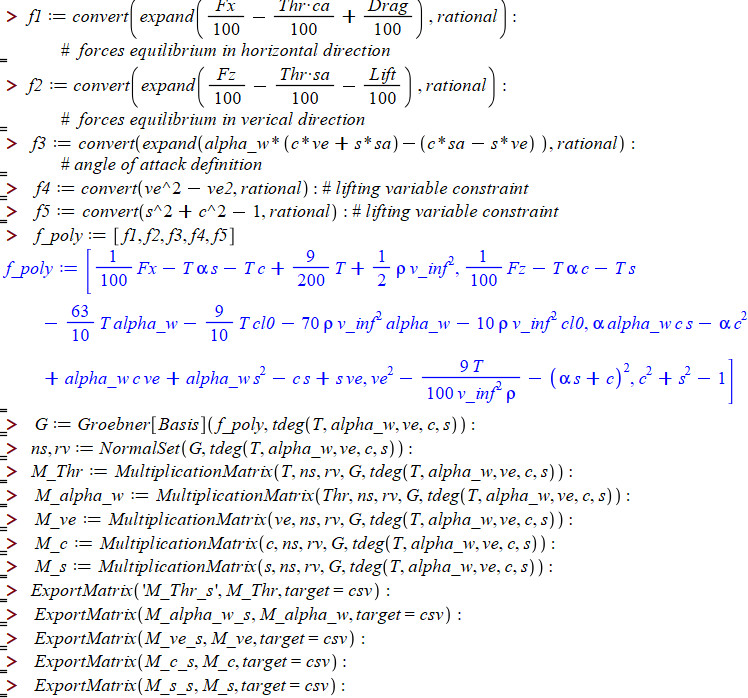
Figure 6: Maple script for generating multiplication matrices.

The multiplication matrices $M_{k}$ are computed once and for all. Their entries are explicit rational functions of the parameters $(v_{\infty},\rho,\alpha_{\infty},cl_{0})$. Then, for each value of the parameters, the multiplication matrices are evaluated numerically. A random linear combination $M(a)=a_{1}M_{1}+\cdots+a_{n}M_{n}$ has distinct unit eigenvectors $v_{1},\ldots,v_{N}$ such that $(v^{T}_{l}M_{k}v_{l})_{k=1,\ldots,n}\in{\mathbb{C}}^{n}$ is a point of $V$, i.e. a solution $x=(T,s,c,v_{i,w})$ of our polynomial equations, for $l=1,\ldots,N$. From these $N$ complex solutions, we then sort out only those with zero imaginary part and which are physically relevant.

The five multiplication matrices of sizes 14x14 are exported into Matlab to calculate their eigenvalues, which correspond to the solution values of inputs and lifting variables. With the algorithm implemented with Matlab we can achieve computation speed well within 10ms on a standard laptop, as shown in Figure 7. The computation speed and the precisely computed solution seem promising towards real-time implementation.

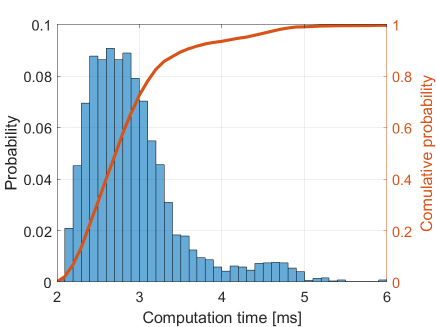
Figure 7: Computation time of the control allocation algorithm, tested in Matlab on a standard laptop. The maximal computation time is below 8ms with a median value of 2.5ms.

The control allocation accuracy was tested using a Monte-Carlo campaign with $10^{6}$ simulation runs and paremeter ranges $v_{\infty}\in[15,20]$ m$\cdot$s^-1, $\rho\in[0.5,1.225]$ kg$\cdot$m^-3, $\alpha_{\infty}\in[5,10]$ deg, $F_{x}\in[40,80]$ N and $F_{z}\in[70,140]$ N. As the control allocation design model, the polynomial reformulation of the forward map (27)-(31) was used, relying on Assumption 1 and Assumption 2. In turn, the full trigonometric forward map (21)-(22) was used for validation of control allocation accuracy, see Figure 8.

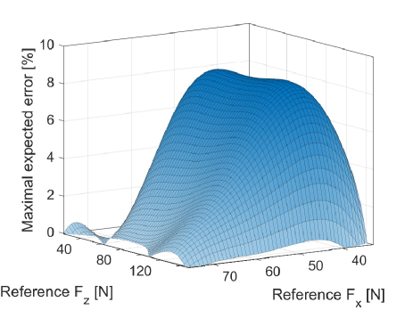
Figure 8: Maximal relative error of control allocation algorithm for Monte-Carlo-type simulations.

Relative allocation error is smaller than 8% for all considered cases.

5 Conclusion

A new control allocation procedure has been proposed for tilt-rotor aircraft. The method allows the flight stabilization, control and guidance algorithms to command the forces acting on the aircraft directly, as the virtual inputs.The allocation procedure relies on state-of-the-art propeller / wing interaction model, addopted from control-focused tilt-wing models. The model inversion is computed with Groebner-bases algorithms. The accuracy of allocated forces is above 90% throughout the flight envelope and computation time is well below 10ms on an average laptop, which makes the method suitable for real-time implementation.

Following the promising results of this paper, we plan to focus on extensive experimental testing of the control allocation method. We plan to parametrize the mathematical model through high-fidelity CFD simulations. Such modifications do not affect the results of this paper as the model inversion method is sufficiently general to be applied to various models with similar complexity. The control allocation algorithm is to be tested on more representative hardware in combination with complete control algorithms to verify the real-time compliance of the approach.

6 ACKNOWLDGEMENT

This work was supported by the Grant Agency of the Czech Technical University in Prague, grant No. SGS22/166/OHK3/3T/13

References

- [1] L. Bauersfeld and G. Ducard. Fused-PID control for tilt-rotor VTOL aircraft. Mediterranean Conference on Control and Automation (MED), pages 703–708, 2020.
- [2] L. Bauersfeld, L. Spannagl, G. Ducard, and C. Onder. MPC flight control for a tilt-rotor VTOL aircraft. IEEE Transactions on Aerospace and Electronic Systems, 57(4):2395–2409, 2021.
- [3] J. Belák and M. Hromčík. Unified attitude control strategy for tilt-rotor vtol aircraft. In American Control Conference (ACC). IEEE, 2023.
- [4] J. Berthomieu, C. Eder, and M. Safey El Din. msolve: A library for solving polynomial systems. Proceedings of ISSAC, Saint-Petersbourg, 2021.
- [5] J. M. Buffington and D. F. Enns. Lyapunov stability analysis of daisy chain control allocation. Journal of Guidance, Control, and Dynamics, 19(6):1226–1230, 1996.
- [6] D. A. Cox, J. Little, and D. O’Shea. Using Algebraic Geometry. Springer, 2nd edition edition, 2007.
- [7] R. de Vries, N. van Arnhem, T. Sinnige, R. Vos, and L. L. M. Veldhuis. Aerodynamic interaction between propellers of a distributed-propulsion system in forward flight. Aerospace Science and Technology, 118:107009, 2021.
- [8] G. Droandi, G. Gibertini, D. Grassi, G. Campanardi, and C. Liprino. Proprotor–wing aerodynamic interaction in the first stages of conversion from helicopter to aeroplane mode. Aerospace Science and Technology, 58:116–133, 2016.
- [9] D.Rohr, T. Stastny, S. Verling, and R. Siegwart. Attitude and cruise control of a VTOL tiltwing UAV. IEEE Robotics and Automation Letters, 4(3):2683–2690, 2019.
- [10] G. J. J. Ducard and M. Allenspach. Review of designs and flight control techniques of hybrid and convertible VTOL UAVs. Aerospace Science and Technology, 118:107035, 2021.
- [11] Ohad Gur and Aviv Rosen. Propeller performance at low advance ratio. Journal of Aircraft, 42(2), 2005.
- [12] C. Kim and J. Chung. Aerodynamic analysis of tilt-rotor unmanned aerial vehicle with computational fluid dynamics. Journal of Mechanical Science and Technology, 20(4):561–568, 2006.
- [13] Z. Kukelová, M. Bujnak, and T. Pajdla. Polynomial eigenvalue solutions to minimal problems in computer vision. IEEE Trans. Pattern Analysis and Machine Intelligence, 34(7):1381–1393, 2012.
- [14] R. Nederlof. Improved modeling of propeller-wing interactions with a lifting-line approach. Phd. thesis, Delft University of Technology, 2020.
- [15] D. Rohr, M. Studiger, T. Stastny, N. R. J. Lawrance, and R. Siegwart. Nonlinear model predictive velocity control of a VTOL tiltwing UAV. IEEE Robotics and Automation Letters, 6(3):5776–5783, 2021.
- [16] X. Shi, K. Kim, S. Rahili, and S. Chung. Nonlinear control of autonomous flying cars with wings and distributed electric propulsion. IEEE Conference on Decision and Control (CDC), pages 5326–5333, 2018.
- [17] B. L. Stevens, F. L. Lewis, and E. N. Johnson. Aircraft control and simulation.
- [18] G. A. M. Van Kuik. The Fluid Dynamic Basis for Actuator Disc and Rotor Theories: Revised Second Edition. IOS Press.
- [19] X. Wang and L. Cai. Mathematical modeling and control of a tilt-rotor aircraft. Aerospace Science and Technology, 47:473–492, 2015.