FADE: Why Bad Descriptions Happen to Good Features

Abstract

Recent advances in mechanistic interpretability have highlighted the potential of automating interpretability pipelines in analyzing the latent representations within LLMs. While they may enhance our understanding of internal mechanisms, the field lacks standardized evaluation methods for assessing the validity of discovered features. We attempt to bridge this gap by introducing FADE: Feature Alignment to Description Evaluation, a scalable model-agnostic framework for evaluating feature-description alignment. FADE evaluates alignment across four key metrics — Clarity, Responsiveness, Purity, and Faithfulness — and systematically quantifies the causes for the misalignment of feature and their description. We apply FADE to analyze existing open-source feature descriptions, and assess key components of automated interpretability pipelines, aiming to enhance the quality of descriptions. Our findings highlight fundamental challenges in generating feature descriptions, particularly for SAEs as compared to MLP neurons, providing insights into the limitations and future directions of automated interpretability. We release FADE as an open-source package at: https://github.com/brunibrun/FADE.

FADE: Why Bad Descriptions Happen to Good Features

Bruno Puri^1,2,*, Aakriti Jain^1,*, Elena Golimblevskaia^1,*, Patrick Kahardipraja¹, Thomas Wiegand^1,2,3, Wojciech Samek^1,2,3, Sebastian Lapuschkin^{1 1}Department of Artificial Intelligence, Fraunhofer Heinrich Hertz Institute, Berlin, Germany ²Department of Electrical Engineering and Computer Science, Technische Universität Berlin, Berlin, Germany ³BIFOLD - Berlin Institute for the Foundations of Learning and Data, Berlin, Germany ^*contributed equally corresponding authors: {wojciech.samek,sebastian.lapuschkin}@hhi.fraunhofer.de

1 Introduction

Understanding the latent features of machine learning models and aligning their descriptions with human-comprehensible concepts remains a crucial challenge in AI interpretability research. Recent advances have made significant strides in this direction, by introducing automated interpretability methods Bills et al. (2023); Bykov et al. (2024); Choi et al. (2024), that leverage larger language-capable models to describe the latent representations of smaller models Bykov et al. (2023); Templeton et al. (2024); Dreyer et al. (2025). This facilitates inspection of ML models, enabling a deeper understanding of models’ behaviour. Consequently, this enhances our ability to identify or mitigate harmful responses and biases, thus improving model transparency and interpretability Lee et al. (2024); Gandikota et al. (2024).

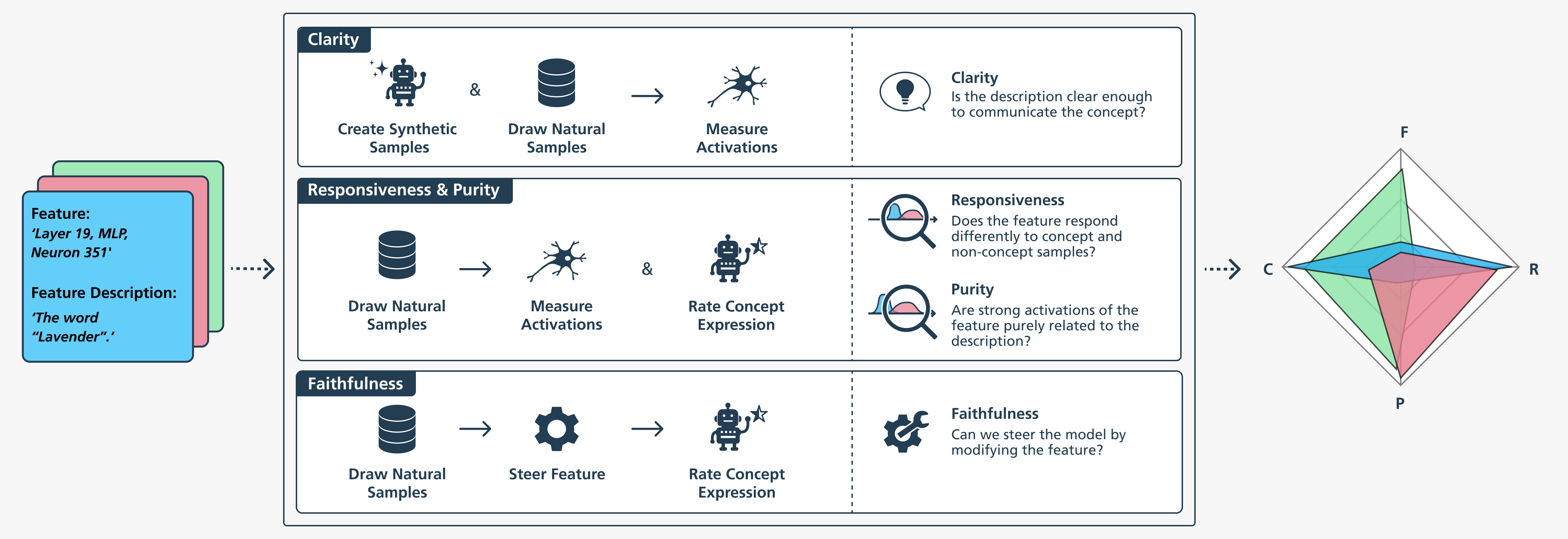
Figure 1: Visualization of the FADE pipeline for three features and their corresponding feature descriptions.

A key insight from these investigations is the highly polysemantic nature of individual neurons — they rarely correspond to single, clear concepts. This discovery has led to the development and adoption of sparse autoencoders (SAEs) McGrath et al. (2024); Bricken et al. (2023); Rajamanoharan et al. (2024), which are intended to decompose polysemantic representations by separating neuron activations into more interpretable components. While SAEs offer a promising approach for feature decomposition, their reliability remains an open question. Recent research reveals significant variability in the way SAEs capture the underlying learned features Heap et al. (2025); Paulo and Belrose (2025), thus highlighting the need for a holistic framework for the evaluation of feature-description alignment. To the best of our knowledge, there is an absence of widely accepted quantitative metrics for evaluating the quality and effectiveness of open-vocabulary feature descriptions. Different methodologies rely on custom evaluation criteria which makes it challenging to conduct meaningful, generalizable comparisons across techniques. Additionally, existing evaluation approaches typically optimize for a single metric Bills et al. (2023); Choi et al. (2024) which may not capture the full complexity of a feature’s behavior and leaves open questions about whether the model truly encodes the hypothesized concept rather than simply correlating with the measured feature. With our work, we contribute as follows:

[1] We present a robust automated evaluation framework designed for broad applicability across model architectures and their SAE implementations.FADE combines four metrics that allow quantitative analysis of different aspects of alignment between features and their generated descriptions.

[2] Through systematic empirical analysis, we provide insights into how various components of the autointerpretability pipeline — such as the number of layers, sample sizes, and architectural choices — affect the quality of feature descriptions.

[3] We release a selected subset of feature descriptions, presented as a part of this work for Gemma-2-2b and Gemma Scope SAEs along with their evaluations.

2 Related Work

Evaluating the alignment between features and their descriptions has become increasingly important with the rise of automated interpretability approaches. While manually inspecting highly activating examples remains a common method to validate interpretations and demonstrate automated interpretability techniques Bills et al. (2023); Templeton et al. (2024), more scalable tools are needed for thorough quantitative evaluation. Many automated or semi-automated approaches have been proposed, generally falling into activation-centric and output-centric methods.

Activation-centric methods focus on measuring how well a feature’s activations correspond to its assigned description.

One prominent approach is a simulation-based scoring, where an LLM predicts feature activations based on the description and input data, and the correlation between predicted and real activations of a feature is measured Bills et al. (2023); Bricken et al. (2023); Choi et al. (2024). While elegant, this approach can be computationally expensive and tends to favor broad, high-level explanations.

A related and conceptually more straightforward way to measure how well the description explains a feature’s behavior is to try to directly generate synthetic samples using the description and compare the resulting activations between concept and non-concept samples Huang et al. (2023); Kopf et al. (2024); Gur-Arieh et al. (2025); Shaham et al. (2025). However, generated datasets are typically small (on the order of 5–20 samples Huang et al. (2023); Gur-Arieh et al. (2025)) and often constrained to rigid syntactic structures or focus only on the occurence of particular tokens, making them less effective for evaluating abstract or open-ended language concepts Huang et al. (2023); Foote et al. (2023).

Another strategy is rating individual samples from a natural dataset for how strongly they express a concept and compare those ratings to the feature’s activations Huang et al. (2023); Paulo et al. (2024); Templeton et al. (2024).

A common limitation of activation-centric methods is that they primarily evaluate positively correlated activations while ignoring negatively encoded neurons, effectively ignoring negatively encoded features Huang et al. (2023); Kopf et al. (2024).

Output-centric methods instead assess how feature activations influence model behavior. Some approaches measure the general decrease in performance of the model after ablating the feature Bills et al. (2023); Makelov et al. (2024), while others use steering-based interventions, where an increase in generated outputs containing the concept is used as a proxy for feature alignment Paulo et al. (2024); Gur-Arieh et al. (2025).

There is a growing need for frameworks that integrate multiple perspectives to provide a comprehensive assessment of feature-to-description alignment across different interpretability methods.

For instance, prior work Bills et al. (2023); Menon et al. (2025); Gur-Arieh et al. (2025) has shown that while activation-centric and output-centric measures often correlate, they do not necessarily imply a causal relationship.

Some studies focus exclusively on SAEs McGrath et al. (2024); Paulo et al. (2024), while others analyze MLP neurons Bills et al. (2023); Choi et al. (2024). Developing an architecture-agnostic framework for feature-to-description evaluation is essential for enabling robust quantitative comparisons across interpretability approaches.

Although efforts have been made to integrate multiple evaluation perspectives Paulo et al. (2024); Gur-Arieh et al. (2025), these remain fragmented and are often too narrowly scoped to handle open-ended language descriptions.

Our work addresses these limitations by introducing a more comprehensive evaluation framework that combines activation- and output-centric metrics while explicitly considering interpretability for open-ended language descriptions.

3 Evaluating Feature Explanations

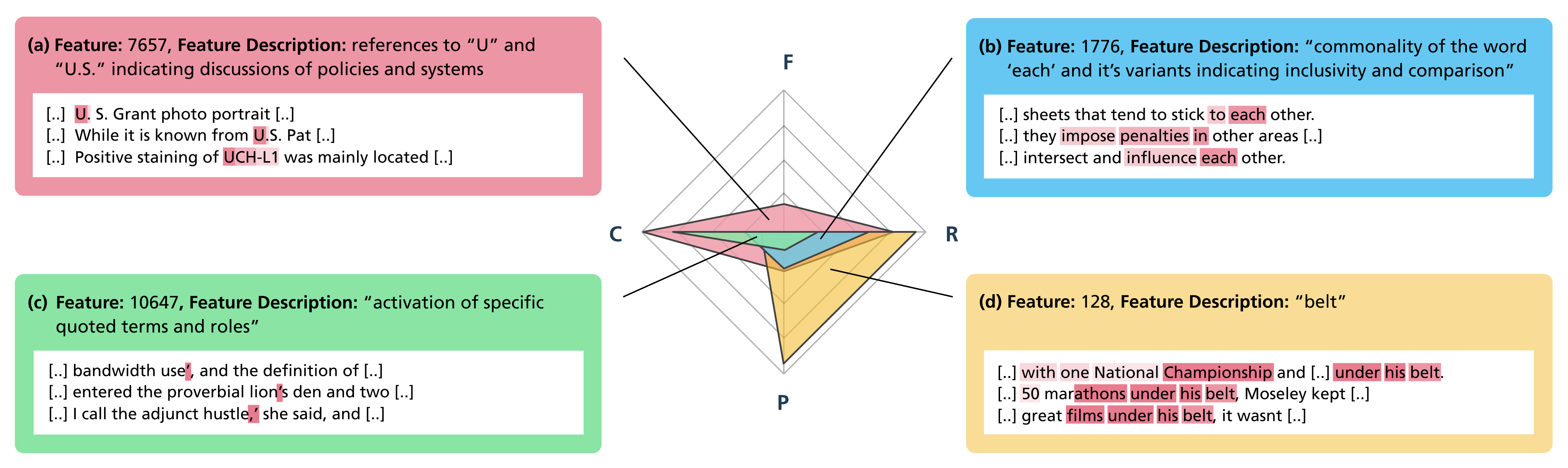
Figure 2: FADE can highlight different problems that arise with description generation. (a) Feature 128 contains concept of the expression “under someone’s belt”. However, the derived concept “belt”, is not clear/ specific enough to be useful for generating synthetic data, that would activate the feature. However, the description is still very close to the concept, therefore Responsiveness and Purity are high. (b) Feature 1776 strongly reacts to the word “each”, but also to many other general, unrelated words, resulting in lower Clarity and Purity. (c) The description for feature 7657 catches its main concept, low Purity indicates that this feature is clearly polysemantic. (d) Description for feature 10647 is expressed too broad, resulting in low Responsiveness and Purity.

Our primary objective is to establish a comprehensive framework that automatically evaluates feature descriptions across a variety of feature types without human intervention. Our framework encompasses four distinct metrics: Clarity, Responsiveness, Purity, and Faithfulness, which we consider necessary and sufficient for assessing the alignment between a feature and its description. In our opinion, such a comprehensive evaluation framework is necessary to ensure that features encode the ascribed concept in a robust way. As feature descriptions are often generated by optimizing for a single metric, such as maximizing the activations of specific neurons, they do not necessarily generalize well to other quantifiable aspects, such as faithfulness Bills et al. (2023); Choi et al. (2024).

We base our approach on four key assumptions. First, we adopt a \footnotesize1⃝ Binary Concept Expression model, whereby a concept is either present in a text sequence or absent. Second, we assume \footnotesize2⃝ Concept Sparsity, i.e. that a given concept appears only rarely in natural datasets, though a sufficiently large dataset will contain some representative examples. Third, we assume \footnotesize3⃝ Feature Reactivity, meaning, when a feature encodes a concept, its activations are significantly stronger on samples that express the concept. This will be valid especially for SAEs, since by construction, for most samples, their activations are zero. This is a strong assumption, as it also implies that a feature should activate strongly only for a single concept. Note, however, that this does not require strict monosemanticity Bricken et al. (2023). In our framework a feature might encode multiple, even entirely unrelated topics, as long as its feature description fully describes all of them. Unlike traditional monosemanticity, which assumes features should directly align with a single human-interpretable category, our framework evaluates interpretability based on whether the feature description accurately reflects the feature’s truly encoded concept, rather than enforcing human-aligned conceptual boundaries. Assumption \footnotesize1⃝ and \footnotesize3⃝ allow us to interpret the activations of a feature as output of a “classifier” of the encoded concept, which can then be easily evaluated. For our metrics, we expect a feature to encode the concept linearly in its activations. Finally, we assume \footnotesize4⃝ Causality - a feature is expected to causally influence the model’s output so that modifying its activation will lead to predictable changes in the generation of concept-related content. These four assumptions will not always hold but are necessary simplifications for now.

3.1 Evaluation Framework Components

Our evaluation framework consists of three main components: A subject LLM, that contains the features we want to evaluate, a natural dataset, that ideally should be close to the LLM training data distribution and is sufficiently large to contain all the concepts, of which the descriptions we want to evaluate, and an evaluating LLM, an open- or closed-source LLM that is used for automating the evaluation process. The evaluating LLM is used for “human-like” inference tasks, such as rating the strength of concept expression in samples and creating synthetic concept data.

3.2 Evaluation Metrics

Clarity

evaluates whether a feature’s description is precise enough to generate strongly activating samples. We assess this by prompting the evaluating LLM to generate synthetic samples based on the feature description (see prompts in Appendix D.2.1). Unlike Gur-Arieh et al. (2025), which generates non-concept sequences artificially, we sample them uniformly from the natural dataset to avoid unnatural biases (i.e. by asking the evaluating LLM not to think about pink elephants). If a feature is well explained by its description, the synthetic concept samples should elicit significantly stronger activations than non-concept samples. We quantify this separability using the absolute Gini coefficient

$$\mathrm{G_{abs}}(A_{c},A_{n})=\left|2\cdot\left(\frac{\sum\limits_{a_{c}\in A_{c}}\sum\limits_{a_{n}\in A_{n}}\mathbf{1}_{[a_{c}>a_{n}]}}{\|A_{c}\|_{0}\cdot\|A_{n}\|_{0}}\right)-1\right|$$ (1)

where $A_{c}$ and $A_{n}$ are the sets of concept and non-concept activations, respectively. Since this metric focuses on linear separability rather than precision, it remains robust even when concept samples occasionally appear within the natural dataset. A low clarity score indicates that either the description is not precise enough to be useful, or might simply be unfitting for the feature, resulting in similar activations for both concept and non-concept samples. For example, in Figure 2, feature (d) responds to “having something under one’s belt,” yet is inaccurately described as “belt”. Conversely, a high clarity score confirms that we can effectively generate samples that elicit strong activations in the feature, although it does not guarantee that the feature is monosemantic or causally involved.

Responsiveness

evaluates the difference in activations between concept and non-concept samples. We select samples from the natural dataset based on their activation levels, drawing both from the highest activations and from lower percentiles (details in Appendix D.1). Following an approach similar to Templeton et al. (2024), we prompt the evaluating LLM to rate each sample on a three-point scale to indicate how strongly the concept is present (0 = not expressed, 1 = partially expressed, 2 = clearly expressed). By discarding the ambiguous (partially expressed) cases, we effectively binarize samples into concept and non-concept categories. We compute the responsiveness score again using the absolute Gini coefficient. A low responsiveness score indicates that activations of concept-samples are similarly strong as non-concept samples, while a high score indicates that, in natural data, samples with strong activations reliably contain the concept.

Purity

is computed using the same set of rated natural samples as responsiveness, but with a different focus: it evaluates whether the strong activations are exclusive to the target concept. In contrast to Huang et al. (2023), who measure recall and precision for a single threshold, we measure the purity using the Average Precision (AP)

$$\mathrm{AP}(A_{c},A_{n})=\sum_{j}\left(r_{j}-r_{j-1}\right)\cdot p_{j}$$ (2)

where $r_{j}$ is the recall and $p_{j}$ is the precision computed at threshold $j$, for each possible threshold, based on $A_{c}$ and $A_{n}$. The AP penalizes instances where non-concept samples also trigger high activations. A purity score near one thus indicates that the feature’s activations are highly specific to the concept, whereas a score near zero suggests that top activations occur for other unrelated concepts as well. This is, for example, the case in polysemanticity, where a feature responds to multiple unrelated concepts.

Faithfulness

addresses the causal relationship between a feature and the model’s output. In other words, it tests whether direct manipulation of the feature’s activations can steer the model’s output toward generating more concept-related content. To evaluate faithfulness, we take random samples from the natural dataset and have the subject LLM generate continuations while applying different modifications to the feature’s activation. For neurons, we multiply the raw activations by a range of factors, including negative values, so that we do not impose a directional bias on how the concept is encoded. For SAE features, of which the activations are more sparse, we first determine the maximum activation observed in the natural dataset Templeton et al. (2024) and then scale this value by the different modification factors. After generating the modified continuations, the evaluating LLM rates how strongly the concept appears in each output. We quantify the strength of this causal influence by measuring the largest increase we were able to steer the model in producing concept-related outputs

$$\mathrm{Faithfulness}(\mathbf{R})=\dfrac{\max(\max(\mathbf{R})-R_{0},0)}{1-R_{0}}$$ (3)

where $\mathbf{R}$ is a vector capturing the proportion of concept-related outputs for each modification factor, and $R_{0}$ denotes the base case in which the feature is “zeroed out” (i.e., multiplied by zero). A faithfulness score of zero implies that manipulating the feature does not increase the occurrence of concept-related outputs, while a score of one indicates that for some modification factor the concept is produced in every continuation.

4 Experiments

In this section, we apply FADE to assess the quality of descriptions generated for various state-of-the-art feature descriptions Choi et al. (2024); Lieberum et al. (2024). Our goal is to demonstrate that the proposed framework provides a robust, multidimensional measure of feature to feature description alignment.

Experimental Setup

As a natural dataset for the evaluations we use samples drawn from the test partition of the Pile dataset Gao et al. (2020), preprocessed as shown in Appendix B. As evaluating LLM we use the OpenAI model gpt-4o-mini-2024-07-18 unless stated otherwise. Prompts for the evaluating LLM as well as details on the hyperparameters can be found in Appendix D.2. We run the experiments on $10^{3}$ randomly chosen features from a single layer of a model: layer 20 for Gemma-2-2b Riviere et al. (2024), layer 20 of Gemma Scope SAEs Lieberum et al. (2024), and layer 19 of Llama-3.1-8B-Instruct Dubey et al. (2024) (see Appendix C.1 for details). The evaluation results have a high variance, which is caused by both the inherent difficulty of interpreting some features as well as the quality of the ascribed feature descriptions. Therefore the mean values are demonstrated only if they aid the analysis of metrics distributions. For all of the presented tables we demonstrate the full distributions as kernel-density estimations with bandwidth adjustment factor 0.3 in Appendix 6.

Automated interpretability approach

Feature descriptions, which we refer to as MaxAct*, are generated based on samples of the train partition of the Pile dataset, that demonstrate maximum activation on the feature, similarly to methods utilized in Bills et al. (2023); Paulo et al. (2024); Rajamanoharan et al. (2024), that we refer to as MaxAct. The minor differences between MaxAct and MaxAct* are prompts, optimized on qualitative analysis provided via FADE, and preprocessing steps of the dataset. The automated interpretability pipeline is described in Appendix C.1.

4.1 Depth and Reliability of Evaluations

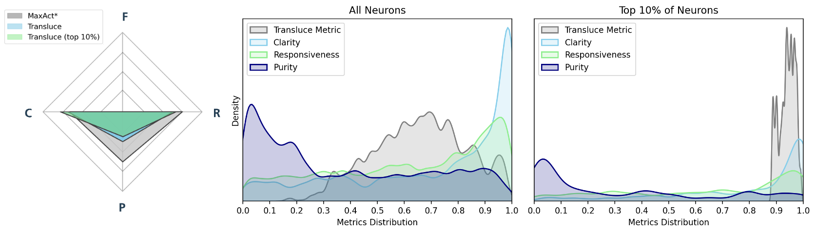
Figure 3: Distribution of metrics in FADE framework and a simulation-based metric on a uniformly subsampled set of features and the top 10% of subsampled features, selected based on the simulated activation metric generated in Choi et al. (2024) (right), and comparison to the proposed descriptions for these features, generated in this work (left).

Limitations of single-metric approaches

We compare FADE with simulated-activation-based metrics Bills et al. (2023); Templeton et al. (2024); Choi et al. (2024), that, while computationally efficient, fail to fully capture the feature-to-description alignment, potentially overlooking critical issues like polysemanticity. To illustrate this, we analyze feature descriptions of Llama-3.1-8B-Instruct generated in Choi et al. (2024). As shown in Figure 3, despite high simulated-activation scores, FADE identifies many features with low purity. Moreover, comparing the average results across all subsampled features with the top 10% of features based on the simulated-activation metric, we find only a marginal gain in clarity and responsiveness, while the purity worsens. Via MaxAct*, we generate descriptions with slightly lower clarity but significantly higher responsiveness and purity. We attribute this to the explainer model in Choi et al. (2024) being fine-tuned on descriptions optimized for the simulated-activation metric, which aligns more closely with clarity but neglects responsiveness and purity.

Better models provide better evaluations

As the evaluating LLM is one of the most computationally expensive components of our framework, selecting a model that balances performance and cost is critical. Larger models generally achieve better performance, but at significantly higher computational costs. To determine a minimal feasible model size and capability required for effective evaluation, we conduct a quantitative analysis of concept-expression ratings across various open-weight and proprietary models, using GPT-4o as a baseline due to its superior benchmark performance OpenAI (2024). We evaluate models on Neuronpedia Lin (2023) feature descriptions for the Gemma Scope SAEs, generated via MaxAct method Rajamanoharan et al. (2024). By comparing deviations in concept strength ratings between GPT-4o and other models, we assess their relative performance (see Table 1).

Model	Class 0	Class 1	Class 2	Valid
GPT-4o	243,233	24,766	19,716	100
Llama-3.2-1B	63.8	22.1	20.9	8.8
Llama-3.2-3B	77.4	9.9	70.3	72.2
Llama-3.1-8B	82.0	14.6	85.6	82.8
Llama-3.3-70B 4q	88.7	31.5	92.6	88.3
GPT-4o mini	93.4	44.8	79.3	88.6

Table 1: Concept rating procedure for different evaluating LLMs. The GPT-4o baseline shows the number of occurrences per class. The other models show their alignment with the GPT-4o rating in percent. The “Valid” column shows the percentage of samples that were correctly classified. Class 0 represents no alignment with the concept, class 1 a partial alignment and class 2 means the samples clearly exhibits the concept.

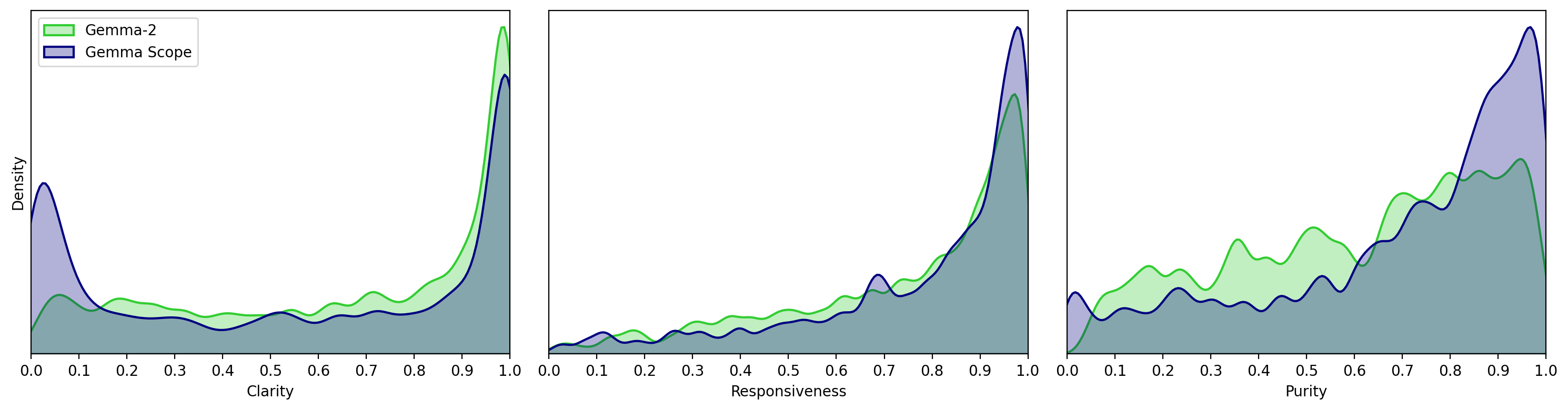
Figure 4: Feature description fit for neuron-based features (Gemma-2) and SAE-based features (Gemma Scope).

Our findings reveal a clear trend: larger, more capable models consistently yield better evaluations. The open-weight Llama-3.3-70B-Instruct (AWQ 4-bit quantized) performs comparably to the proprietary GPT-4o mini, a widely used model in autointerpretability research Choi et al. (2024); Lin (2023). While Class 1 (partial alignment) is the most error-prone, smaller models, such as Llama-3.2-3B-Instruct, remain viable for the more critical Class 0 (no alignment) and Class 2 (strong alignment). However, for optimal performance, models smaller than Llama-3.1-8B-Instruct are likely insufficient.

Generating feature descriptions for SAEs is more challenging than for MLP neurons

To compare MLP neurons and SAE features, we analyze Gemma-2-2b and Gemma Scope SAEs. While Gemma-2 outperforms Gemma Scope SAEs in average clarity (see Table 4), the clarity score distribution reveals a left-skewed peak for SAEs, as depicted on Figure 4. Further analysis identifies a cluster of features with low clarity but moderate to high responsiveness and purity. These features have descriptions that approximate the encoded concept but lack the precision to strongly activate the SAE feature (see (d) in Figure 2). This suggests that despite greater monosemanticity, interpreting SAE features remains challenging due to the difficulty of generating precise descriptions. In contrast, responsiveness and purity are higher on average for SAEs, as these metrics are less sensitive to imprecise descriptions and still align with the underlying concept. The higher purity in SAEs aligns with their increased monosemanticity.

SAE Size	Clarity	Respon-siveness	Purity	Faithfulness
MaxAct* 16K	0.57	0.78	0.69	0.17
MaxAct* 65K	0.46	0.71	0.66	0.15
Neuronpedia 16K	0.43	0.67	0.60	0.17
Neuronpedia 65K	0.29	0.64	0.56	0.13

Table 2: Comparison results for SAEs of different sizes, see metrics distributions on Figure 5.

Interpreting larger SAEs is more difficult

We investigate whether SAEs with a higher number of features inherently exhibit a better alignment with the feature descriptions. To quantify this, we compare feature descriptions from Gemma Scope 16K and Gemma Scope 65K. We compare it based on Neuronpedia feature descriptions, as well as the ones obtained in this work via MaxAct*. Consistent with our previous finding, our results indicate that increasing the number of SAE features does not inherently improve the alignment of features with their descriptions, as shown in Table 2. We hypothesize that this stems from a finer-grained decomposition of concepts, making it more challenging for the explainer LLM to capture and articulate the precise concept.

Layer	Clarity	Respon-siveness	Purity	Faithfulness
3	0.60	0.71	0.55	0.009
12	0.44	0.54	0.43	0.016
20	0.67	0.74	0.61	0.011
25	0.59	0.65	0.54	0.025

Table 3: Evaluation results for different layers in Gemma-2, see metrics distributions on Figure 6.

Interpretability varies across layers

Table 3 presents an evaluation of feature descriptions from different layers of Gemma-2-2b. Our analysis identifies layer 12 as the most challenging to interpret. A manual inspection of 50 randomly sampled features confirms these results: features in layer 12 exhibit high polysemanticity. The highest scores are observed in layer 20, with the exception of the faithfulness metric. However, this may be due to the fine-tuning of the MaxAct* approach on this layer, which introduces a bias that specifically affects faithfulness. The highest faithfulness score is observed in layer 25, while the lowest is found in layer 3.

4.2 Evaluating Autointerpretability: Prompts, Examples, and Model Size

Despite the growing number of methods proposed in automated interpretability research, there has been surprisingly little comprehensive evaluation of different approaches. In this section, we present a series of experiments that assess different components of feature generation pipelines and demonstrate how FADE can help in fine-tuning interpretability pipelines.

Prompting with numerical- or delimiter-based input

Prompt construction can significantly influence the quality of the generated descriptions. We investigate two primary approaches: passing (word, activation) pairs and using {{delimiters}} to highlight the most activated tokens (see Appendix C.2 for more details). Our experiments indicate that the numerical input performs slightly better than the delimiter-based prompt, which contradicts previous research Choi et al. (2024).

Model	Input type	Clarity	Respon-siveness	Purity	Faithfulness
Gemma-2	delimiters	0.67	0.74	0.61	0.01
	numeric	0.67	0.76	0.64	0.01
Gemma Scope	delimiters	0.57	0.78	0.69	0.16
	numeric	0.59	0.80	0.72	0.17

Table 4: Comparison results of activations input types via delimiters vs numerical input, see metrics distributions on Figure 7 (a).

Few-shot prompting improves description quality

Next we test how many examples should be passed to the explainer model in the prompt. We compare 0-shot (without examples), 1-shot, 2-shot, 5-shot, 10-shot and 20-shot prompts on Gemma Scope. In these variations, we use the delimiter-based prompts. The results, provided in Table 5, demonstrate, that a larger number of examples brings steady improvement in clarity, responsiveness and purity. Faithfulness shows no clear trend.

Number of shots	Clarity	Respon-siveness	Purity	Faithfulness
0-shot	0.53	0.76	0.70	0.17
1-shot	0.55	0.76	0.68	0.19
2-shot	0.57	0.78	0.69	0.17
5-shot	0.60	0.79	0.72	0.16
10-shot	0.60	0.79	0.72	0.16
20-shot	0.61	0.81	0.73	0.16

Table 5: Comparison results for different number of shots provided to the explainer model with the prompt based on Gemma Scope, see metrics distributions on Figure 7 (c).

Providing more samples increases evaluation scores

We test 5, 15 and 50 samples, using the same delimiter-based prompts (see Table 6). The results indicate, that increasing the number of samples improves description quality, though the gains are not substantial for any of the tested number of samples.

Model	# samples	Clarity	Respon-siveness	Purity	Faithfulness
Gemma2	5	0.63	0.72	0.59	0.01
	15	0.67	0.74	0.61	0.01
	50	0.69	0.77	0.62	0.01
Gemma Scope	5	0.56	0.77	0.67	0.17
	15	0.57	0.78	0.69	0.18
	50	0.60	0.79	0.71	0.17

Table 6: Comparison results for different number of activating samples provided to the explainer model, see metrics distributions on Figure 7 (b).

Better models produce better feature descriptions

Similarly to the experiment, comparing different evaluation models presented in Table 1, we compare different explainer models and demonstrate the results in Table 7. GPT-4o achieves the highest scores, with Llama-3.3-70B-Instruct (AWQ 4-bit quantized) and GPT-4o mini as close alternatives. The smaller models struggle with assigning reasonable feature descriptions, in particularly Llama-3.2-1B, which frequently fails to maintain a consistent response structure (see Appendix 6).

Model	Clarity	Respon-siveness	Purity	Faithfulness
Llama-3.2-1B	0.39	0.56	0.35	0.10
Llama-3.2-3B	0.51	0.73	0.61	0.15
Llama-3.1-8B	0.50	0.75	0.66	0.17
Llama-3.3-70B	0.54	0.78	0.70	0.19
GPT-4o mini	0.58	0.78	0.70	0.17
GPT-4o	0.61	0.80	0.73	0.17

Table 7: Explainer models comparison, see metrics distributions on Figure 8.

Baselines fail in predictable ways

To assess the effectiveness of MaxAct* approach, we compare it against established baseline methods, including the Neuronpedia feature descriptions, a TF-IDF Ramos et al. (2003); Salton and Buckley (1988) based description approach, and an unembedding-based method Joseph Bloom (2024) (see Appendix C.1 for methodological details). The results are presented in Table 8. MaxAct* consistently outperforms baselines in clarity, responsiveness, and purity. Notably, the unembedding method achieves the highest faithfulness score, a result that aligns with our expectations and related work Gur-Arieh et al. (2025). Since this method explicitly considers the output that a given feature promotes, it naturally excels at capturing causal influence of the feature. However, this focus on output consistency often comes at the expense of clarity, responsiveness, and purity, as raw unembedding-based descriptions do not incorporate any information about what activates the feature. These findings again highlight the necessity of a holistic evaluation framework, as different methods optimize for different aspects of interpretability.

Approach	Clarity	Respon-siveness	Purity	Faithfulness
Neuronpedia	0.43	0.67	0.60	0.21
TF-IDF	0.42	0.72	0.53	0.21
Unembedding	0.38	0.65	0.61	0.29
MaxAct*	0.57	0.78	0.69	0.21

Table 8: Comparison of the quality of our feature descriptions to baselines, see metrics distributions on Figure 9.

5 Conclusion

In this work, we presented FADE, a new automated evaluation framework designed to rigorously evaluate the alignment between features and their open-vocabulary feature descriptions. By combining four complementary metrics Clarity, Responsiveness, Purity, and Faithfulness, our approach gives a comprehensive assessment of how a feature reacts to instances of the described concept, an evaluation of the description itself as well as the feature’s causal role in the model’s outputs. Through extensive experiments across different feature types, layers, and description generation mechanisms, we demonstrated that methods relying on a single metric (e.g., simulation-based approaches) often give incomplete or misleading feature descriptions. Our framework can be used to highlight both the strengths and weaknesses of existing methods, while it also helps in debugging and improving these methods. We highlighted multiple results for improving the quality of feature explanations, such as using larger, more capable LLMs for the explainer and including more examples in the prompt. We hope that the open-source implementation of FADE will drive further research in automated interpretability and help make language models more transparent and safe to use.

Limitations

Despite presenting a comprehensive and robust evaluation framework, our work has certain limitations that we want to highlight here: One key limitation is the potential biases in the LLMs used for both rating and synthetic data generation. These biases can affect the evaluation process and perpetuate biases, especially in automated interpretability. For instance, an LLM might recognize a feature encoding a concept in English as directly representing that concept, whereas the same feature in another language might be classified with the additional specification of the language. This discrepancy could lead to unintended biases when steering models based on these interpretations. Similar issues may arise from biases present in the pre-training datasets used in our evaluation procedure. Another limitation is related to the steering behavior in the faithfulness pipeline. Our current implementation does not explicitly verify whether the generated sequences under modification remain grammatically correct and semantically meaningful. However, minor modifications to the prompt could potentially address this issue in the future. Finally, our faithfulness measure is not well-suited for handling inhibitory neurons. A neuron may causally inhibit the presence of a concept in a model’s output, but our metric, by design, does not effectively capture decreases in the appearance of sparse concepts. This limitation arises both from the definition of our faithfulness metric and the inherent challenges in measuring such suppression effects for already sparse concepts.

Appendix A Extended related work

A common approach to automatic interpretability includes selecting data samples that strongly activate a given neuron and using these samples, along with their activations as input to a larger LLM, that serves as an explainer model and generates feature descriptions Bills et al. (2023); Bricken et al. (2023); Choi et al. (2024); Paulo et al. (2024); Rajamanoharan et al. (2024). Previous research has investigated various factors influencing this method, including prompt engineering, the number of data samples used, and the size of the explainer model (see Appendix A).

Building on this approach, Choi et al. (2024) advanced the method by fine-tuning Llama-3.1-8B-Instruct on the most accurate feature descriptions, as determined by their simulated-activation metric. This fine-tuning aimed to improve the performance and accuracy of description generation, ultimately outperforming GPT-4o mini.

An output-centric approach was introduced by Gur-Arieh et al. (2025) in an attempt to address another key challenge-the feature descriptions generated via the data samples that activate the feature the most, often fail to reflect its influence on the model’s output. The study demonstrates that a combined approach, integrating both activation-based and output-based data, results in more accurate feature descriptions and improves performance in causality evaluations.

Several studies perform their experiments exclusively on SAEs McGrath et al. (2024); Paulo et al. (2024); Rajamanoharan et al. (2024); Templeton et al. (2024), while others focus on MLP neurons Bills et al. (2023); Choi et al. (2024). Although Templeton et al. (2024) compares the interpretability of SAEs to that of neurons and concludes that features in SAEs are significantly more interpretable, these findings heavily rely on qualitative analyses.

Previous research consistently shows that open-source models are effective for generating explanations, with advanced models producing better descriptions. For instance, Bills et al. (2023) report that GPT-4 achieves the highest scores, whereas Claude 3.5 Sonnet performs best for Paulo et al. (2024). The number of data samples used to generate feature description also varies across studies. Bills et al. (2023) use the top five most activating samples, while Choi et al. (2024) select 10-20 of the most activating samples to generate multiple descriptions for evaluation. In contrast, Paulo et al. (2024) use 40 samples and suggests that randomly sampling from a broader set of activating leads to descriptions that cover a more diverse set of activating examples, whereas using only top activating examples often yields more concise descriptions which fails to capture the entire description.

The datasets used in these studies also differs. Paulo et al. (2024) utilize the RedPajama 10M Computer (2023) dataset, Choi et al. (2024) use the full LMSYSChat1M Zheng et al. (2023) and 10B token subset of FineWeb Penedo et al. (2024), and Bills et al. (2023) — on WebTextRadford et al. (2019) and the data used to train GPT-2 Radford et al. (2019). Additionally, different delimiter conventions are observed: Choi et al. (2024) use delimiters, Paulo et al. (2024) use << >>, and Bills et al. (2023) use numerical markers.

Appendix B Data Preprocessing

For our work, we used an uncopyrighted version of the Pile dataset, with all copyrighted content removed, available on Hugging Face Gao et al. (2020) (https://huggingface.co/datasets/monology/pile-uncopyrighted). This version contains over 345.7 GB of training data from various sources. From this dataset, we extracted approximately 6 GB while preserving the relative proportions of the original data sources. The extracted portion from the training partition was used to collect the most activated samples. For evaluations, we utilized the test partition from the same dataset, applying identical preprocessing steps as those used for the training data.

Component	Size (GB)	Proportion (%)
Pile-CC	1.93	32.17
PubMed Central	1.16	19.38
ArXiv	0.70	11.67
FreeLaw	0.55	9.14
PubMed Abstracts	0.32	5.39
USPTO Backgrounds	0.31	5.23
Github	0.27	4.54
Gutenberg (PG-19)	0.23	3.85
Wikipedia (en)	0.15	2.57
DM Mathematics	0.11	1.87
HackerNews	0.07	1.17
Ubuntu IRC	0.06	0.99
EuroParl	0.06	0.95
PhilPapers	0.03	0.58
NIH ExPorter	0.03	0.50
Total	5.99	100.00

Table 9: Extracted dataset and proportion of sub components

Our preprocessing involved several steps to ensure a balanced and informative dataset. First, we used the NLTK Bird et al. (2009) sentence tokenizer to break large text chunks into individual sentences. We then filtered out sentences in the bottom and top fifth percentiles based on length, as these were typically out-of-distribution cases consisting of single words or characters or a few outliers. This step helped achieve a more balanced distribution. Additionally, we removed sentences containing only numbers or special characters with no meaningful content. Finally, duplicate sentences were deleted.

	Training	Test
Number of sentences	88,689,425	5,443,427
Number of tokens	2,284,636,243	137,600,815
Number of unique tokens	21,707,092	2,336,552

Table 10: Dataset Statistics

Appendix C Automated Interpretability Pipeline

C.1 Implementation of Automated Interpretability

Model	Layers	HuffingFace	Descriptions
Gemma-2-2b	3, 12, 20, 25	google/gemma-2-2b	–
Gemma Scope 16K	20	google/gemma-scope-2b-pt-res/tree/main/ layer_20/width_16k/average_l0_71	neuronpedia.org/gemma-2-2b/20-gemmascope-res-16k
Gemma Scope 65K	20	google/gemma-scope-2b-pt-res/tree/main/ layer_20/width_65k/average_l0_114	neuronpedia.org/gemma-2-2b/20-gemmascope-res-65k
Llama3.1-8B-Instruct	19	meta-llama/Llama-3.1-8B-Instruct	github.com/TransluceAI/observatory.git

Table 11: Sources for models, SAEs and feature descriptions, used in this work.

Our experiments are based on models and feature descriptions presented in Table 11. We generate our feature descriptions as follows. In the implementation of the autointerpretability pipeline, we’re closely following Bills et al. (2023); Paulo et al. (2024); Rajamanoharan et al. (2024) and others: we pass the natural dataset, used for generating descriptions (see Appendix B) through the model, and via forward hooks we access the activations of each feature and each layer. This part can also be easily parallelized. With Gemma Scope SAEs, a wrapper class is implemented, that is built into the model as another module. It can be extended easily to other SAEs.

After passing the whole dataset through the model, for each feature we take top $10^{3}$ data samples based on the maximum activation of tokens. We only consider the maximum activating token of a data sample when we do the sorting. Later, we uniformly subsample the necessary number of data samples, i.e. 5, 15, …, 50, that are further passed to an explainer LLM.

The reason why we subsample from top $10^{3}$ is to avoid outliers in terms of activation. Top $10^{3}$ still represents top 0.001% of the dataset. More complex sampling strategies can bring better performance, as described in Appendix A, but their implementation and evaluation is left out for the future work.

Experiments are performed on the following models: Gemma-2-2b layer 20 Riviere et al. (2024), Llama-3.1-8B-Instruct layer 19 Dubey et al. (2024), and SAEs Gemma Scope 16K and 65K layer 20 Lieberum et al. (2024). We also generate descriptions using baseline methods, namely TF-IDF and unembedding matrix projection. Term Frequency-Inverse Document Frequency (TF-IDF) is a widely used technique in NLP for measuring the importance of a word in a document relative to a corpus. It balances word frequency with how uniquely the word appears across documents, assigning higher scores to informative words while down-weighting common ones. We generate these values using 15 maximally activating samples. On the other hand, the unembedding matrix ($W_{U}$) Joseph Bloom (2024) in transformer models maps the residual stream activations to vocabulary logits, determining word probabilities in the output. By analyzing projections onto this unembedding matrix, we gain insight into how learned features influence token predictions. To generate SAE unembedding descriptions, we generate logit weight distribution across the vocabulary, and then use the top ten words with the highest probabilities as feature description.

$$\text{Logit weight distribution}=W_{U}*W_{dec}[feature]$$

here, $W_{U}$ is the unembedding matrix of a transformer model and $W_{dec}$ are the decoder weights of sparse auto encoders.

This reveals which words are most associated with a given feature, enabling interpretability of sparse autoencoder (SAE) features, as well as MLP neurons. Both these methods are cheap baselines to compare with different auto-interpretability generated descriptions.

C.2 Prompts Engineering

Our feature description pipeline consists of several key components. The Subject Model for which the descriptions are getting generated, while the Explainer Model is a larger model used to generate descriptions. The System Prompt provides task-specific instructions to the LLM, detailing what to focus on in the provided samples and how to format the output. We append 5, 10, or 50 sentences along with a user_message_ending at the end, which helps reinforce the expected output structure. Before normalizing activations, we first average activations for tokens belonging to the same word. These values are then normalized between 0 and 10. For delimiters, we use single curly brackets if the activation intensity is below 4 and double curly brackets otherwise. For numerical input, we provide the LLM with dictionary of most activated token at the end of each sample.

	Avg # of tokens	Cost/$10^{3}$ feature ($)
0-shot	1,423	2.13
1-shot	1,498	2.25
2-shot	1,564	2.35
10-shot	2,395	3.95
20-shot	3,393	5.09

Table 12: Token usage and cost comparison for different shot settings.

# of sentences	Avg # of tokens
5	333
15	964
50	2,507

Table 13: Average number of tokens as the number of sentences increases. These values are based on tokenizer used for Gemma-Scope-16k and are not the number of tokens per requests generated by openai.

Main prompt: The main prompt for our we use to generate descriptions is given below:

⬇

You are a meticulous AI researcher conducting an important investigation into sparse autoencoders of a language model that activates in response to specific tokens within text excerpts. Your overall task is to identify and describe the common features of highlighted tokens, focusing exclusively on the tokens that activate and ignoring broader sentence context unless absolutely necessary.

You will receive a list of sentences in which specific tokens activate the neuron. Tokens causing activation will appear between delimiters like {{ }}. The activation values range from 0-10:

- If a token activates with an intensity of <4, it will be delimited like {{this}}.

- If a token activates with an intensity of >4, it will be delimited like {{{{this}}}}.

Guidelines:

1. Focus on the activated tokens: The description must primarily relate to the highlighted tokens, not the entire sentence.

2. Look for patterns in the tokens: If a specific token or a group of similar tokens repeatedly activates, center your analysis on them.

3. Sparse Autoencoder Dependency: The activations depend only on the words preceding the highlighted token. Descriptions should avoid relying on words that come after the activated token.

4. No coherent presence of concept: Return ’NO CONCEPT FOUND’ if there is no coherent theme in the sentences provided, do not force a concept and stay grounded.

Output Format:

Concept: [Focus on the common concept tied to the highlighted tokens, described in a concise phrase.]

### Example:

Input example 1:

Sentence 1: The {{United States}} will not allow {{threats}} against its people.

Sentence 2: The {{U.S.}} emphasizes deterrence in foreign policy.

Example Output:

Concept: U.S. deterrence policies and moral stance on global threats.

Input example 2:

Sentence 1: Ash/Brock [Bouldershipping]\nI forget about this one {{all}} for one favours.

Sentence 2: I see this attitude brewing {{all}} at once.

Sentence 3: I get emails from people {{all}} over the world.

Example Output:

Concept: Presence of the word ’all’.

user_message_ending: >

Analyze all these sentences as ONE corpus and provide your description in the following format:

Concept: Your devised concept and it’s description in a concise manner, and very few words.

Prompt variation 1: using numbers, instead of delimiters for further experiments as mentioned in , we include small variations in the main prompt

⬇

You are a meticulous AI researcher [...]

You analyze a list of most-activated sentences and a dictionary of relevant tokens, each with assigned activation values, to identify key themes and concepts. Tokens causing activations will be provided in the dictionary after each sentence. The activation values range from 0-10.

Guidelines:[..]

Output Format:

Concept: [Focus on the common concept tied to the highlighted tokens, described in a concise phrase.]

EXAMPLE 1

Sentence 1: "The choir’s harmonies resounded throughout the church as the congregation stood in awe."

Most relevant tokens: {{"harmonies": 9, "resounded": 8, "church": 6, "congregation": 4}}[..]

Prompt variation 2: main prompt + no shotsc
Prompt variation 3: main prompt + one shot example
Prompt variation 4: main prompt + five shots

C.3 Computational Costs

Obtaining maximum activating samples for features is performed locally on a cluster with 8 NVIDIA A100 GPUs with VRAM 40Gb. The process can be easily parallelized, but for cost calculation we are using the total consumed time. Such GPUs can be rented starting with $0.67/hr, however, an average price on the market exceeds this value. For simplicity of calculations, we take a price of $1/hr. For convenience, we consider a price per $10^{3}$ features, the results are presented in Table 14.

	# of features	Time (h)	Cost/$10^{3}$ features ($)
Gemma-2-2b	239,616	185	0.77
Gemma Scope 16K	16,384	524	31.98
Gemma Scope 65K	65,536	622	9.49
Llama-3.1-8B	458,752	361	0.79

Table 14: Cost comparison for discovering samples, that are maximally activating features.

Due to the differences in the implementation, calculating maximum activating samples is significantly cheaper for the complete models, since we are doing it at the same moment for the whole model, and the price is divided on the total number of features that we consider. For SAEs, in the current implementation we only do it per one layer, which is significantly reducing the number of considered features. In the future we are planning on optimizing this process in a way, that it is possible to calculate it at the same time for multiple chosen SAEs. The size of SAEs is also playing an important role: in terms of total costs it is more expensive, but if we consider the cost per $10^{3}$ features, the larger the SAE - the cheaper it is.

The total computational cost for this part of the experiments is estimated at 4,920 GPU hours. This includes all experiments conducted on the models referenced in this paper. While not all experiments are explicitly discussed, they contributed to the final results presented here.

Appendix D FADE Evaluation Framework

Our framework is designed to work with a wide variety of subject models, including most HuggingFace Transformers (Wolf et al., 2020) as well as any feature implemented as a named module in PyTorch. Moreover, our framework is extensible: interpretability tools such as SAEs or various supervised interpretability techniques can be integrated with minimal effort, provided they implement some basic steering functions. In addition, we offer an interface for a diverse set of evaluating LLMs, whether open-weight or proprietary, with support for platforms such as vllm, Ollama, OpenAI, and Azure APIs. Our implentation can be found at https://github.com/brunibrun/FADE.

D.1 Implementation and Computational Efficiency

To compute the purity and responsiveness measures, we base our sampling from the natural dataset on the activations of the subject LLM. For each sequence, we calculate the maximum absolute activation value across all tokens. Using these values, we sample sequences by selecting a user-configurable percentage of those with the strongest activations and for the remainder, drawing an equal number of samples from each of the following percentile ranges: $[0\%,50\%[$, $[50\%,75\%[$, $[75\%,95\%[$, and $[95\%,100\%]$.

Computational efficiency is a key consideration in our design, as evaluating every neuron in an LLM can be prohibitively expensive. The cost of evaluations is dynamically adjustable based on several factors, including the number of samples generated and rated, the evaluating LLM used, and the natural dataset selection.

Our method allows users to control the cost by setting the number of synthetic samples (denoted $n$) relative to the full size of the natural dataset ($N$). By pre-computing activations from the natural dataset in parallel, we effectively reduce the per-run complexity from $\mathcal{O}(N*M)$ for $M$ neurons to $\mathcal{O}(n*M)$. Given that $n$ is typically in the hundreds while $N$ is in the millions, this strategy yields big efficiency gain.

Additionally, we only execute the computationally intensive faithfulness evaluation when both clarity and responsiveness exceed a user-configurable threshold. This conditional execution ensures that unnecessary computations are avoided for features that do not meet our interpretability criteria.

D.2 Details on the Experiment Setup

In our experiments we send 15 requests to the evaluation LLM for generating synthetic samples. We remove duplicates and use these as concept-samples. We use the whole evaluation dataset as control samples. For rating we draw 500 samples from the natural dataset, where we take 50 from the top activated and 450 from the lower percentiles, according to the sampling strategy outlined above in Appendix D.1. If we obtain fewer than 15 concept-samples in this first rating we again sample 500 new samples with the same sampling approach. We rate 15 samples at once, and if one of the calls fails, for example due to formatting errors of the evaluating LLM, we retry the failed samples once. For the Faithfulness experiments we use the modification factors $[-50,-10,-1,0,1,10,50]$. We draw 50 samples from the natural dataset and let the subject LLM continue them for 30 tokens. We then rate only these continuations for concept strength by the evaluating LLM, again retrying once, if the rating fails. We only execute the Faithfulness experiment, if both the Clarity and Responsiveness of a feature is larger or equal to 0.5.

Licenses Gemma-2-2b is released under a custom Gemma Terms of Use. Gemma Scope SAEs are released under Creative Commons Attribution 4.0 International. Llama3.1-8B-Instruct is released under a custom Llama 3.1 Community License. Transluce feature descriptions, Pile Uncopyrighted dataset and LangChain are released under MIT License. vLLM is released under Apache 2.0 License.

D.2.1 Prompts for the Evaluating LLM

Generating Synthetic Data Prompt

⬇

You are tasked with building a database of sequences that best represent a specific concept.

To create this, you will generate sequences that vary in style, tone, context, length, and structure, while maintaining a clear connection to the concept.

The concept does not need to be explicitly stated in each sequence, but each should relate meaningfully to it. Be creative and explore different ways to express the concept.

Here are examples of how different concepts might be expressed:

Concept: "German language" - Sequences might include German phrases, or sentences.

Concept: "Start of a Java Function" - Sequences might include Java code snippets defining a function.

Concept: "Irony" - Sequences might include ironic statements or expressions.

Provide your sequences as strings in a Python List format.

Example: ["This is a first example sequence.", "Second example sequence but it is much longer also there are somy typos in it. wjo told you that I can type?"]

Output only the Python List object, without any additional comments, symbols, or extraneous content.

Rating Natural Data Prompt

⬇

You are tasked with building a database of sequences that best represent a specific concept.

To create this, you will review a dataset of varying sequences and rate each one according to how much the concept is expressed.

For each sequence, assign a rating based on this scale:

0: The concept is not expressed.

1: The concept is vaguely or partially expressed.

2: The concept is clearly and unambiguously present.

Use conservative ratings. If uncertain, choose a lower rating to avoid including irrelevant sequences in your database.

If no sequence expresses the concept, rate all sequences as 0.

Each sequence is identified by a unique ID. Provide your ratings as a Python dictionary with sequence IDs as keys and their ratings as values.

Example Output: {{"14": 0, "15": 2, "20": 1, "27": 0}}

Output only the dictionary - no additional text, comments, or symbols."

D.2.2 Associated Cost

The activation generation for the subject models for the results in section 4.1 was run locally on a cluster with NVIDIA A100 GPUs with 40GB of VRAM. Similar to section C.3 we assume a price of $1/hr. Since activations can be cached in parallel for the whole model, only a single pass over the evaluation dataset was needed per model. We estimate a needed time of 24 hours on one GPU for the activation generation, resulting in a cost of 24$ per model. During the evaluations, only the activations of synthetic samples need to be computed. Due to a suboptimal configuration of the evaluation and subject LLM in our experiments we assume an average time of one minute per neuron evaluation, leading to an average cost of 0.024$ per evaluated feature. The estimated cost for the evaluating LLM consists of the cost for the generation of synthetic samples as well as the cost for rating natural data. In the configuration used for the experiments, unless stated otherwise, we estimate the evaluating LLM creates about 2,000 tokens per feature evaluation, which corresponds to a cost of about 0.0012$ per feature at an output token cost of 0.6$ per million tokens. For the rating part the evaluating LLM recieves about 20,000 tokens as input, which corresponds to a cost of 0.003$ per feature at an input token cost of 0.15$ per million tokens. Corresponding results are presented in Table 15.

	# of features evaluated	GPU Time (h)	Cost/ $10^{3}$ features($)
Gemma-2-2b	9,000	216 + 24	26.67
Gemma Scope 16K	25,000	600 + 24	24.96
Gemma Scope 65K	2,000	48 + 24	36
Llama-3.1-8B	2,000	48 + 24	36

Table 15: Computational cost comparison for running the evaluation experiments on GPU.

Appendix E Extended Results

E.1 Quantitative Analysis

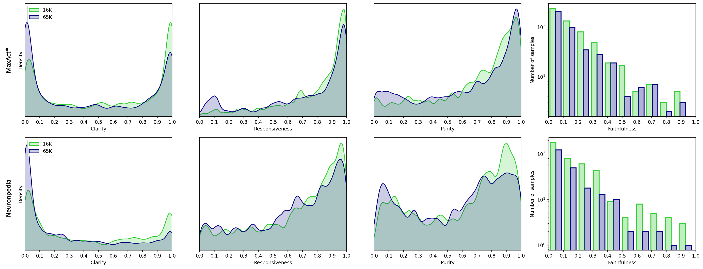
Figure 5: Feature descriptions fit for SAEs of different sizes.

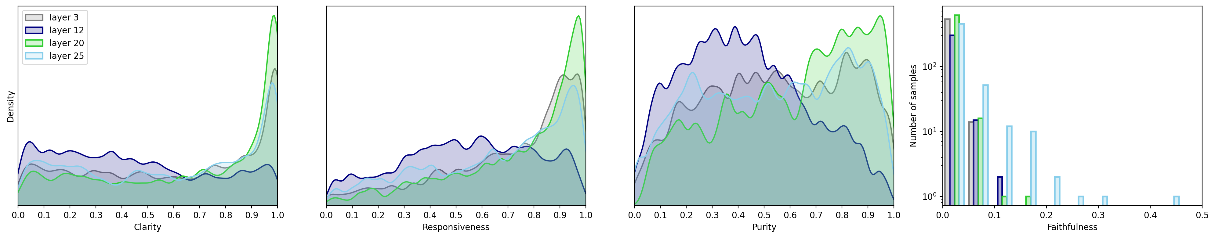
Figure 6: Feature descriptions fit for different layers of Gemma-2.

This section provides a more in-depth analysis of the experimental results presented in Section 4.1.

SAEs concept narrowness results in lower interpretability. This might seem counterintuitive at first, but again it is important to stress that we are not evaluating the features by themselves, but instead the adequacy of the proposed feature description to these features. One potential explanation is that larger SAEs distribute concepts more finely across features. As a result, a slightly inaccurate description that might have still activated a feature in a smaller SAE may fail to activate the corresponding feature in a larger SAE, where concepts are encoded even more sparsely. The consistency of this result is demonstrated by using different feature descriptions — MaxAct*, produced in this work, and the ones available on Neuronpedia.

Interestingly, we observe a small left-skewed peak in the responsiveness distribution for 65K SAEs labelled via MaxAct*, a pattern not seen in any other experiment (see Figure 5). A qualitative analysis suggests that this is primarily caused by features representing out-of-distribution concepts relative to the dataset used for evaluation, such as, e.g., “new line” feature, which due to the preprocessing steps is not present in the dataset used for descriptions generation (see Figure 12). Due to the lower quality of feature descriptions, the purity distribution for Neuronpedia descriptions of Gemma Scope 65K exhibits a bimodal pattern. High-quality descriptions tend to have high purity, reflecting the greater monosemanticity of the features. However, a substantial number of inaccurate descriptions lead to very low purity values.

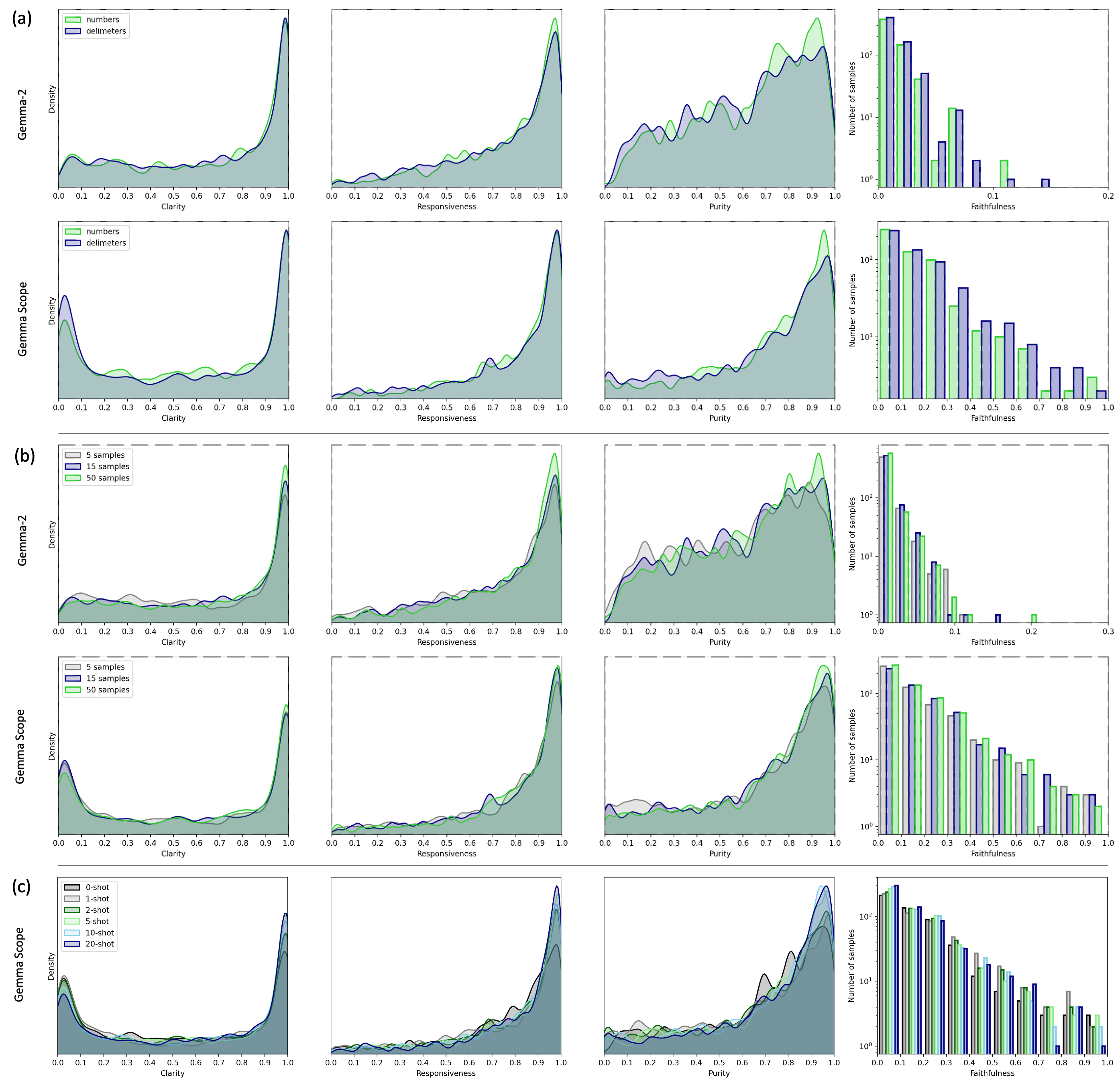
Figure 7: Analysis of the main prompt’s components: (a) numeric input vs delimeter-based; (b) number of activating samples, provided to the explainer LLM; (c) number of shots used in the prompt.

Some Gemma-2 layers look almost not interpretable. The feature distribution in layer 12 differs significantly from other layers. Unlike other layers, layer 12 lacks the characteristic rightward elevation in clarity, responsiveness, and purity scores, as presented on Figure 6. Manual analysis of the heatmaps supported the theory, that layer 12 demonstrates a high level of polysemanticity. Interestingly, similar result was demonstrated on Llama-3.1-8B-Instruct by Choi et al. (2024). Evaluating several complete models with FADE would provide more insights into interpretability of different models components.

Numeric input shows marginally better performance. As illustrated in Figure 7 (a), the performance difference between numeric input-based prompts and delimiter-based highlighting is not statistically significant for both MLP neurons and SAEs, though the mean score is slightly higher for numeric input. A more comprehensive evaluation across multiple layers and a larger feature set is needed to determine the optimal approach. Nonetheless, these findings challenge prior assertions that highlighting the most activating tokens is superior due to LLMs’ assumed difficulty in processing numerical inputs Choi et al. (2024).

Increasing sample count improves performance. A clear trend emerges: providing more samples to the explainer LLM enhances its performance. However, this also increases the computational cost of feature generation due to the higher token count. While 15 samples yield strong results, 50 samples perform even better, as shown in Figure 7 (b).

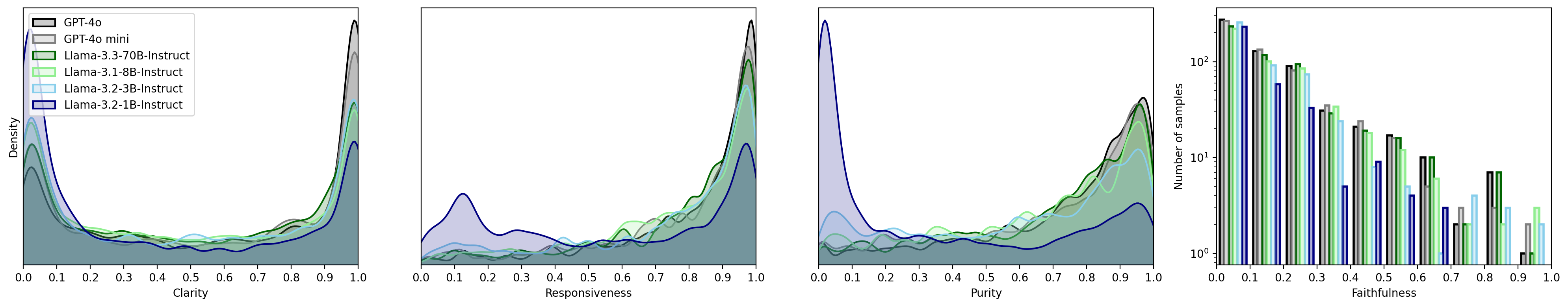
Figure 8: Performance of feature descriptions generation via different explainer LLMs.

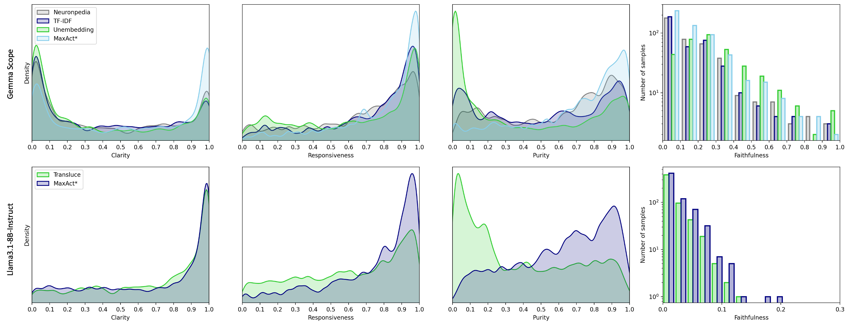
Figure 9: MaxAct* comparison to feature descriptions, generated via other methods on Gemma Scope 16K and Llama3.1-8B-Instruct.

Increasing examples improves performance but raises costs. As shown in Figure 7 (c), increasing the number of shots consistently enhances performance on activation-based metrics without significantly affecting faithfulness, contradicting findings in Choi et al. (2024). This discrepancy may stem from differences in provided examples or feature types, as our analysis focuses on Gemma Scope SAEs, whereas Choi et al. (2024) examined Llama-3.1-8B-Instruct neurons. Additionally, a higher shot count increases computational costs due to the larger token input (see Table 12). In this study, we primarily use 2-shot prompts, balancing performance and cost efficiency.

Stronger explainer LLMs yield better feature descriptions. More capable models consistently achieve higher performance across nearly all metrics, as presented in Figure 8. Llama-3.1-70B-Instruct (quantized) performs comparably to GPT-4o mini, aligning with findings from the evaluation of LLMs (see Table 1). Performance generally declines with model size, except for Llama-3.2-1B-Instruct, which frequently fails to adhere to the required output format, leading to significantly poorer results across all metrics.

MaxAct* demonstrates superior performance. Our findings highlight the importance of considering all four FADE metrics when optimizing automated interpretability approaches. On Gemma Scope 16K, MaxAct* outperforms all baselines across all metrics except faithfulness (see Figure 9). We show that our generated descriptions significantly surpass those currently available on Neuronpedia. Additionally, we compare MaxAct* to TF-IDF and unembedding-based baselines (see Appendix C.1). While the unembedding method underperforms in activation-based metrics such as clarity, responsiveness, and purity, it achieves notably higher faithfulness by explicitly considering the feature’s output behavior. This underscores that faithfulness depends on both the feature type (e.g., SAEs vs. MLP neurons) and the generated description.

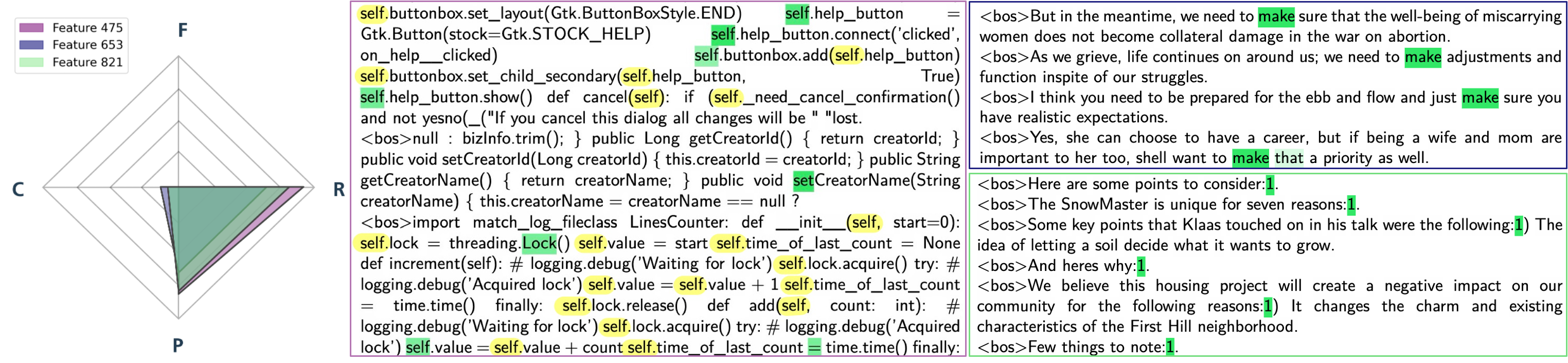
Figure 10: Examples of feature descriptions, obtained via MaxAct*, demonstrating low clarity, but medium or high responsiveness and purity. Feature 475: “Frequent presence of token ’self’ indicating object oriented programming concept”; feature 653: “Word ’make’ in different forms, expressions and concepts”; feature 821: “Expressions indicating lists or explanations”.

Our results align with Gur-Arieh et al. (2025), which demonstrates that combining MaxAct-like approaches with output-based methods enhances overall feature description quality. However, the input-centric metric used in that work does not fully capture failure modes that clarity, responsiveness, and purity account for.

This becomes particularly evident when comparing MaxAct* to feature descriptions generated for Llama-3.1-8B-Instruct in Choi et al. (2024). While clarity scores are comparable—albeit slightly lower for MaxAct* — responsiveness and purity show significant improvements. This difference may partially stem from dataset construction variations. Notably, the purity distributions of the two approaches are strikingly different, even opposing: MaxAct* exhibits a right-skewed peak, whereas Transluce’s feature descriptions perform poorly overall. Faithfulness differences are minor but still favor MaxAct*, likely due to the generation of higher-quality feature descriptions.

E.2 Qualitative Analysis

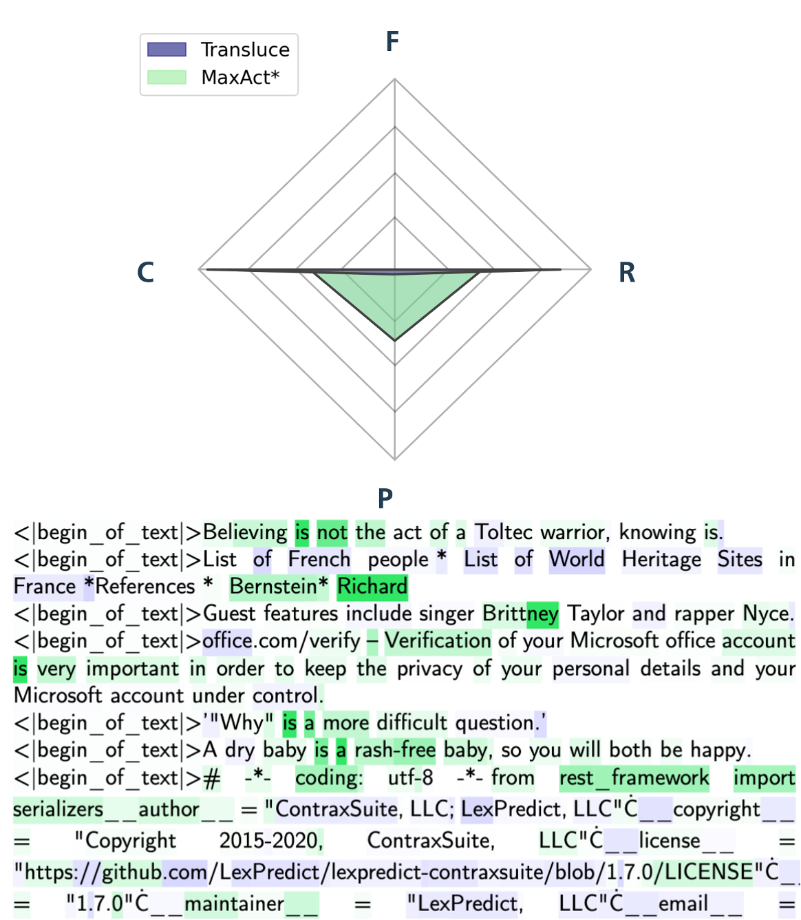
Figure 11: Heatmap and descriptions evaluation result for feature 5183 of Llama3.1-8B-Instruct layer 19.

Method	Label
Transluce	activation on names with specific formatting, including "Bryson," "Brioung," "Bryony," and "Brianna"
MaxAct*	Presence and significance of the word "is"

Table 16: Descriptions for Llama3.1-8B-Instruct feature 5183 layer 19.

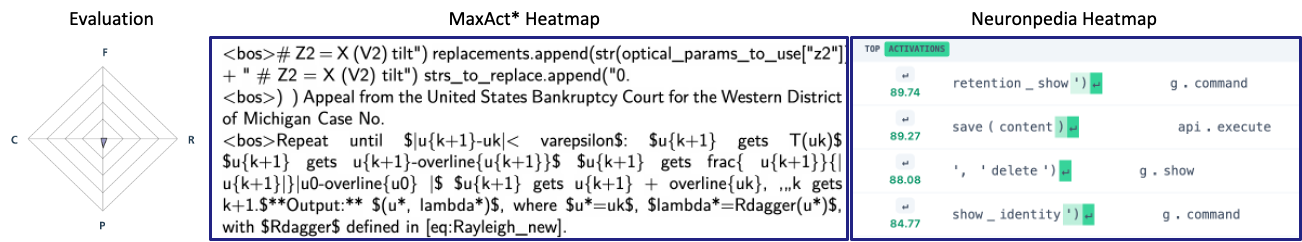
Figure 12: Feature 3,286 of Gemma Scope 65K SAE. MaxAct* description: “Mathematical expressions and significant numerical values”. Neuronpedia description: “function definitions in a programming context”.

Fine-tuning automated interpretability requires consideration of all metrics in FADE. The comparison of metric distributions against the simulated activation-based metric in Figure 3 highlights that relying solely on this metric is insufficient for accurately assessing the quality of feature descriptions. If an automated interpretability framework is fine-tuned exclusively on such a metric, it may generate suboptimal descriptions.

For instance, evaluations indicate that the description for feature 5183 in layer 19 of Llama3.1-8B-Instruct, as generated in Choi et al. (2024), performs well in terms of clarity and responsiveness, yet achieves a near-zero purity score (see Figure 11). Conversely, a description produced using MaxAct* (see Table 16) exhibits lower clarity and responsiveness but significantly higher purity.

The heatmap of activations during description generation suggests that the description from Choi et al. (2024) strongly activates this feature. While the heatmap does not show all the names listed in Transluce’s description, this may be due to the sampling method, which selects random sentences from the top 1000 to mitigate outliers. However, activation is observed on similar names, such as “Bernstein” and “Brittney.” More importantly, this clearly polysemantic feature responds to multiple distinct concepts, including the word “is” in specific contexts (included into a description generated via MaxAct*), as well as certain coding patterns.

As a result, despite the relatively high metric score of 0.77 in Transluce’s evaluation, the description has very low purity. This underscores the importance of considering not only how well a concept activates a feature but also other interpretability factors measurable with FADE. In this case, although the feature is inherently difficult to interpret, we argue that the MaxAct* description provides a more accurate representation, as it better captures the feature’s activating pattern, and FADE is clearly demonstrating the feature’s polysemanticity.

SAEs descriptions often fail to accurately capture the concept. Figure 10 presents the heatmap for feature 475, whose description emphasizes the occurrence of the token “self.” However, the feature does not activate on all instances of “self” (highlighted in yellow), indicating that a crucial aspect of the concept is missing or remains unclear. Additionally, the feature activates on other tokens, further suggesting that the description is incomplete.

This is reflected in the evaluation metrics: low clarity indicates that the concept is not expressed precisely enough for the evaluating LLM to generate synthetic data that reliably activates the feature. A responsiveness score of 0.93 suggests that the feature does activate on natural data aligned with the concept, while a purity score of 0.81 reveals that although the feature is primarily associated with the described concept, it also responds to other inputs.

Similar issues arise in features 653 and 821, where the underlying concepts appear highly specific – activating on a particular token within a specific context. However, their descriptions are overly broad, making it difficult to generate synthetic data that reliably triggers the feature. These and many other similar features contribute to the left-skewed peak in the clarity distribution, which becomes more pronounced for narrower concepts represented by features in Gemma Scope 65K.

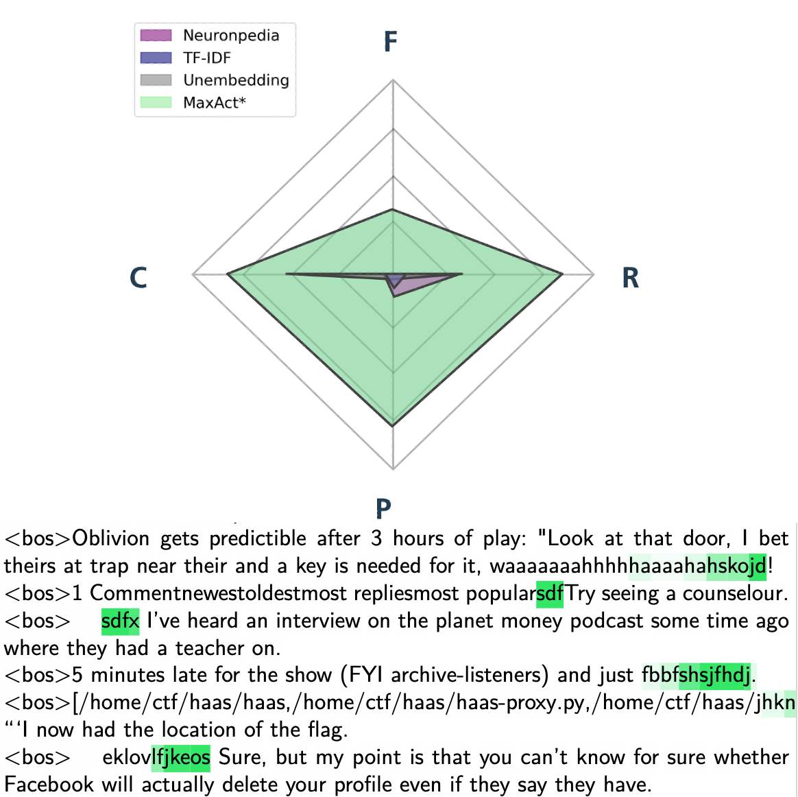
Figure 13: Heatmap and descriptions evaluation result for feature 9295 of Gemma Scope layer 20.

Method	Label
Neuronpedia	The presence of JavaScript code segments or functions
TF-IDF	asdfasleilse asdkhadsj easy file jpds just mean span think
Unembedding	f, <eos>, fd, wer, sdf, df, b, jd, hs, ks
MaxAct*	Presence of nonsensical or random alphanumeric strings

Table 17: Descriptions for Gemma Scope feature 9295 layer 20.

Out-of-Distribution Features in Gemma Scope 65K SAEs. The dataset used for automatic interpretability omitted certain concepts, such as "new line," leading to gaps in feature descriptions. These omissions contribute to the small left-side peak in responsiveness distribution in Figure 5. Several features, including 3315, 3858, and 4337, lack activation heatmaps under the MaxAct* approach, as the dataset does not represent their concepts. Consequently, the explainer model, relying on unrelated sentences, generates incorrect descriptions (see Figure 12). Heatmaps from Neuronpedia reveal what would activate these features, highlighting limitations of the dataset, used in this work, and broader issues in the automated interpretability pipeline. For example, despite obtaining and visualizing correct results, feature descriptions available on Neuronpedia are also not representing a correct concept. Similar results have been obtained for the <bos> token and indentation in text and code.

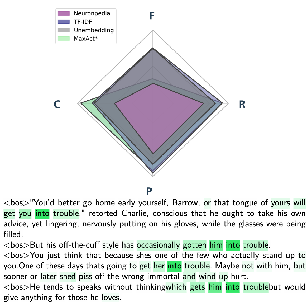
Figure 14: Heatmap and descriptions evaluation result for feature 1139 of Gemma Scope layer 20.

Method	Label
Neuronpedia	references to problematic situations or conflicts that cause trouble
TF-IDF	trouble
Unembedding	troubles, difficulties, problems, troublesome, mischief, …
MaxAct*	Activation of "into" and "trouble" indicating situations leading to problem

Table 18: Descriptions for Gemma Scope feature 1139 layer 20.

Reliable Evaluation — FADE Identifies the Best Description. Different automated interpretability methods prioritize either activation-based metrics or faithfulness-based measures, leading to descriptions that may be overly broad or inaccurate.

In some cases, even manual inspection of heatmaps fails to fully capture the underlying concept represented by a feature. Therefore, a comprehensive evaluation must consider all four metrics.

Table 17 presents feature descriptions generated by various methods. Based on the heatmap analysis, the MaxAct* description most accurately represents the concept. The unembedding method, while incorporating specific tokens promoted by the feature, also demonstrates strong alignment with the concept, as reflected in the corresponding metrics. However, it is not descriptive enough, which is resulting in lower responsiveness and purity.

Sometimes baseline methods may outperform more complex approaches, particularly on specific metrics. For instance, TF-IDF and unembedding baselines exhibit significantly higher faithfulness compared to Neuronpedia or MaxAct* for certain features (see Figure 14).

Feature 1139, for example, influences the output of tokens related to the concept of “trouble”. Descriptions that explicitly capture this aspect tend to achieve higher faithfulness (see Table 18). The MaxAct* description, in contrast, emphasizes the broader meaning and the most activating expression, “into trouble”, leading to higher clarity.

References

- Bills et al. (2023) Steven Bills, Nick Cammarata, Dan Mossing, Henk Tillman, Leo Gao, Gabriel Goh, Ilya Sutskever, Jan Leike, Jeff Wu, and William Saunders. 2023. Language models can explain neurons in language models.
- Bird et al. (2009) Steven Bird, Ewan Klein, and Edward Loper. 2009. Natural language processing with Python: analyzing text with the natural language toolkit. " O’Reilly Media, Inc.".
- Bricken et al. (2023) Trenton Bricken, Adly Templeton, Joshua Batson, Brian Chen, Adam Jermyn, Tom Conerly, Nick Turner, Cem Anil, Carson Denison, Amanda Askell, Robert Lasenby, Yifan Wu, Shauna Kravec, Nicholas Schiefer, Tim Maxwell, Nicholas Joseph, Zac Hatfield-Dodds, Alex Tamkin, Karina Nguyen, Brayden McLean, Josiah E Burke, Tristan Hume, Shan Carter, Tom Henighan, and Christopher Olah. 2023. Towards monosemanticity: Decomposing language models with dictionary learning. Transformer Circuits Thread.
- Bykov et al. (2023) Kirill Bykov, Mayukh Deb, Dennis Grinwald, Klaus-Robert M"uller, and Marina M.-C. H"ohne. 2023. DORA: exploring outlier representations in deep neural networks. Trans. Mach. Learn. Res., 2023.
- Bykov et al. (2024) Kirill Bykov, Laura Kopf, Shinichi Nakajima, Marius Kloft, and Marina H"ohne. 2024. Labeling neural representations with inverse recognition. Advances in Neural Information Processing Systems, 36.
- Choi et al. (2024) Dami Choi, Vincent Huang, Kevin Meng, Daniel D Johnson, Jacob Steinhardt, and Sarah Schwettmann. 2024. Scaling automatic neuron description.
- Computer (2023) Together Computer. 2023. Redpajama: An open source recipe to reproduce llama training dataset.
- Dreyer et al. (2025) Maximilian Dreyer, Jim Berend, Tobias Labarta, Johanna Vielhaben, Thomas Wiegand, Sebastian Lapuschkin, and Wojciech Samek. 2025. Mechanistic understanding and validation of large ai models with semanticlens. Preprint, arXiv:2501.05398.
- Dubey et al. (2024) Abhimanyu Dubey, Abhinav Jauhri, Abhinav Pandey, Abhishek Kadian, Ahmad Al-Dahle, Aiesha Letman, Akhil Mathur, Alan Schelten, Amy Yang, Angela Fan, et al. 2024. The llama 3 herd of models. Preprint, arXiv:2407.21783.
- Foote et al. (2023) Alex Foote, Neel Nanda, Esben Kran, Ionnis Konstas, and Fazl Barez. 2023. N2g: A scalable approach for quantifying interpretable neuron representations in large language models. Preprint, arXiv:2304.12918.
- Gandikota et al. (2024) Rohit Gandikota, Sheridan Feucht, Samuel Marks, and David Bau. 2024. Erasing conceptual knowledge from language models. Preprint, arXiv:2410.02760.
- Gao et al. (2020) Leo Gao, Stella Biderman, Sid Black, et al. 2020. The pile: An 800gb dataset of diverse text for language modeling. Preprint, arXiv:2101.00027.
- Gur-Arieh et al. (2025) Yoav Gur-Arieh, Roy Mayan, Chen Agassy, Atticus Geiger, and Mor Geva. 2025. Enhancing automated interpretability with output-centric feature descriptions. Preprint, arXiv:2501.08319.
- Heap et al. (2025) Thomas Heap, Tim Lawson, Lucy Farnik, and Laurence Aitchison. 2025. Sparse autoencoders can interpret randomly initialized transformers. Preprint, arXiv:2501.17727.
- Huang et al. (2023) Jing Huang, Atticus Geiger, Karel D’Oosterlinck, Zhengxuan Wu, and Christopher Potts. 2023. Rigorously assessing natural language explanations of neurons. In Proceedings of the 6th BlackboxNLP Workshop: Analyzing and Interpreting Neural Networks for NLP, pages 317–331, Singapore. Association for Computational Linguistics.
- Joseph Bloom (2024) Johnny Lin Joseph Bloom. 2024. Understanding sae features with the logit lens.
- Kopf et al. (2024) Laura Kopf, Philine Lou Bommer, Anna Hedstr"om, Sebastian Lapuschkin, Marina M.-C. H"ohne, and Kirill Bykov. 2024. Cosy: Evaluating textual explanations of neurons. In Advances in Neural Information Processing Systems 38: Annual Conference on Neural Information Processing Systems 2024.
- Lee et al. (2024) Andrew Lee, Xiaoyan Bai, Itamar Pres, Martin Wattenberg, Jonathan K Kummerfeld, and Rada Mihalcea. 2024. A mechanistic understanding of alignment algorithms: A case study on dpo and toxicity. Preprint, arXiv:2401.01967.
- Lieberum et al. (2024) Tom Lieberum, Senthooran Rajamanoharan, Arthur Conmy, Lewis Smith, Nicolas Sonnerat, Vikrant Varma, Janos Kramar, Anca Dragan, Rohin Shah, and Neel Nanda. 2024. Gemma scope: Open sparse autoencoders everywhere all at once on gemma 2. In Proceedings of the 7th BlackboxNLP Workshop: Analyzing and Interpreting Neural Networks for NLP, pages 278–300, Miami, Florida, US. Association for Computational Linguistics.
- Lin (2023) Johnny Lin. 2023. Neuronpedia: Interactive reference and tooling for analyzing neural networks. Software available from neuronpedia.org.
- Makelov et al. (2024) Aleksandar Makelov, George Lange, and Neel Nanda. 2024. Towards principled evaluations of sparse autoencoders for interpretability and control. Preprint, arXiv:2405.08366.
- McGrath et al. (2024) Tom McGrath, Daniel Balsam, Myra Deng, and Eric Ho. 2024. Understanding and steering llama 3 with sparse autoencoders.
- Menon et al. (2025) Abhinav Menon, Manish Shrivastava, David Krueger, and Ekdeep Singh Lubana. 2025. Analyzing (in)abilities of saes via formal languages. Preprint, arXiv:2410.11767.
- OpenAI (2024) OpenAI. 2024. Hello GPT-4o.
- Paulo and Belrose (2025) Gonçalo Paulo and Nora Belrose. 2025. Sparse autoencoders trained on the same data learn different features. Preprint, arXiv:2501.16615.
- Paulo et al. (2024) Gonçalo Paulo, Alex Mallen, Caden Juang, and Nora Belrose. 2024. Automatically interpreting millions of features in large language models. Preprint, arXiv:2410.13928.
- Penedo et al. (2024) Guilherme Penedo, Hynek Kydlíček, Loubna Ben allal, Anton Lozhkov, Margaret Mitchell, Colin Raffel, Leandro Von Werra, and Thomas Wolf. 2024. The fineweb datasets: Decanting the web for the finest text data at scale. In The Thirty-eight Conference on Neural Information Processing Systems Datasets and Benchmarks Track.
- Radford et al. (2019) Alec Radford, Jeffrey Wu, Rewon Child, David Luan, Dario Amodei, Ilya Sutskever, et al. 2019. Language models are unsupervised multitask learners. OpenAI blog, 1(8):9.
- Rajamanoharan et al. (2024) Senthooran Rajamanoharan, Tom Lieberum, Nicolas Sonnerat, Arthur Conmy, Vikrant Varma, János Kramár, and Neel Nanda. 2024. Jumping ahead: Improving reconstruction fidelity with jumprelu sparse autoencoders. Preprint, arXiv:2407.14435.
- Ramos et al. (2003) Juan Ramos et al. 2003. Using tf-idf to determine word relevance in document queries. In Proceedings of the first instructional conference on machine learning, volume 242, pages 29–48. Citeseer.
- Riviere et al. (2024) Morgane Riviere, Shreya Pathak, Pier Giuseppe Sessa, Cassidy Hardin, Surya Bhupatiraju, Léonard Hussenot, Thomas Mesnard, Bobak Shahriari, Alexandre Ramé, et al. 2024. Gemma 2: Improving open language models at a practical size. Preprint, arXiv:2408.00118.
- Salton and Buckley (1988) Gerard Salton and Christopher Buckley. 1988. Term-weighting approaches in automatic text retrieval. Information processing and management, 24(5):513–523.
- Shaham et al. (2025) Tamar Rott Shaham, Sarah Schwettmann, Franklin Wang, Achyuta Rajaram, Evan Hernandez, Jacob Andreas, and Antonio Torralba. 2025. A multimodal automated interpretability agent. Preprint, arXiv:2404.14394.
- Templeton et al. (2024) Adly Templeton, Tom Conerly, Jonathan Marcus, Jack Lindsey, Trenton Bricken, Brian Chen, Adam Pearce, Craig Citro, Emmanuel Ameisen, Andy Jones, Hoagy Cunningham, Nicholas L Turner, Callum McDougall, Monte MacDiarmid, C. Daniel Freeman, Theodore R. Sumers, Edward Rees, Joshua Batson, Adam Jermyn, Shan Carter, Chris Olah, and Tom Henighan. 2024. Scaling monosemanticity: Extracting interpretable features from claude 3 sonnet. Transformer Circuits Thread.
- Wolf et al. (2020) Thomas Wolf, Lysandre Debut, Victor Sanh, Julien Chaumond, Clement Delangue, Anthony Moi, Pierric Cistac, Tim Rault, Rémi Louf, Morgan Funtowicz, Joe Davison, Sam Shleifer, Patrick von Platen, Clara Ma, Yacine Jernite, Julien Plu, Canwen Xu, Teven Le Scao, Sylvain Gugger, Mariama Drame, Quentin Lhoest, and Alexander M. Rush. 2020. Transformers: State-of-the-art natural language processing. In Proceedings of the 2020 Conference on Empirical Methods in Natural Language Processing: System Demonstrations, pages 38–45, Online. Association for Computational Linguistics.
- Zheng et al. (2023) Lianmin Zheng, Wei-Lin Chiang, Ying Sheng, Tianle Li, Siyuan Zhuang, Zhanghao Wu, Yonghao Zhuang, Zhuohan Li, Zi Lin, Eric P Xing, et al. 2023. Lmsys-chat-1m: A large-scale real-world llm conversation dataset. arXiv preprint arXiv:2309.11998.