Dynamics of soft interacting particles on a comb

Abstract

We study the dynamics of overdamped Brownian particles interacting through soft pairwise potentials on a comb-like structure. Within the linearized Dean-Kawasaki framework, we characterize the coarse-grained particle density fluctuations by computing their one- and two-point correlation functions. For a tracer particle constrained to move along the comb backbone, we determine the spatial correlation profile between its position and the density of surrounding bath particles. Furthermore, we derive the correction to the diffusion coefficient of the tracer due to interactions with other particles, validating our results through numerical simulations.

• March 5, 2025

1 Introduction

Particles diffusing in complex environments can undergo anomalous diffusion, characterized by a nonlinear growth with time of their mean squared displacement $\expectationvalue{x^{2}(t)}$. The ubiquity of anomalous diffusion in soft and biological systems [1] has, over the past decades, stimulated significant interest in developing minimal theoretical models to capture this behavior [2, 3]. In this context, diffusion of particles in systems with geometrical constraints, such as fractal or disordered lattices, has been the subject of an intense theoretical scrutiny [4, 5], also due to its relevance to the description of transport in porous media, polymer mixtures, and living cells.

Among the simplest inhomogeneous structures is the comb: this can be visualized as a line (called the backbone) spanning the system from one end to the other, and connected to infinite structures (the teeth), as depicted in Fig. 1. Comb structures have been originally introduced to represent diffusion in critical percolation clusters [6, 7, 8], with the backbone and teeth of the comb mimicking the quasi-linear structure and dead ends of the clusters, respectively. In general, one expects that a particle will spend a long time exploring a tooth, resulting in a sub-diffusive motion along the backbone — e.g., $\expectationvalue{x^{2}(t)}\sim t^{1/2}$ in two spatial dimensions [9]. Since then, comb-like models have been used to describe real systems such as cancer proliferation [10] and dendronized polymers [11], transport in spiny dendrites [12], and the diffusion of cold atoms [13] or in crowded media [14].

From a theoretical perspective, the single-particle comb model is sufficiently simple to allow for the derivation of several exact analytical results, both in the continuum [15, 16, 17, 18, 19, 20], and on the lattice [21, 22, 23, 24, 25, 26] — see also Ref. [27] for an overview. By contrast, the many-body problem, consisting of interacting particles evolving on a comb, has received much less attention, and so far restricted to the case of hard-core lattice gases [28, 29, 30, 31]. The natural step forward, which we aim to address here, is to explore the dynamics of interacting particles in continuum space, subject to the comb constraint.

To this end, in this work we consider a system of overdamped Brownian particles interacting via soft pairwise potentials, and constrained to move on a comb, as described in Section 2. Using the Dean-Kawasaki formalism [32, 33], we first derive in Section 3 the exact coarse-grained equations that describe the dynamics of the particle density field $\rho(\mathbf{x},t)$. Expanding the latter around a constant background density, in Section 4 we then derive the one- and two-point functions that completely characterize the density fluctuations within the Gaussian approximation. To the best of our knowledge, this represents the first application of the Dean-Kawasaki theory to non-homogeneous media [34, 35]. Next, in Section 5, we single out a tagged tracer from the bath of interacting particles, assuming that it is constrained to move only along the comb backbone. In this setting, we first derive the spatial correlation profiles that describe the cross-correlations between the tracer position and the surrounding bath density, and then use them to estimate the effective diffusion coefficient of the tracer, which we finally test using Brownian dynamics simulations.

Figure 1: Schematic representation of interacting Brownian particles evolving on a comb structure in $d=2$. Bath particles (blue) can move horizontally along the backbone, or vertically along the teeth. Note that, in the continuum model considered here, the teeth are continuously distributed along the horizontal direction (in the sketch they are instead represented as spatially separated, only for graphical purposes). The tracer particle (red) is constrained to diffuse only along the backbone.

2 The model

We consider a system of $(N+1)$ Brownian particles at positions $\mathbf{r}_{i}(t)$, which evolve according to the overdamped Langevin equations

$$\dot{\mathbf{r}}_{i}(t)=-\hat{\mu}^{(i)}\left(\mathbf{r}_{i}(t)\right)\sum_{j\neq i}\nabla_{\mathbf{r}_{i}}U_{ij}\left(\mathbf{r}_{i}(t)-\mathbf{r}_{j}(t)\right)+\bm{\eta}_{i}\left(\mathbf{r}_{i}(t),t\right),$$ (1)

where the Gaussian noises $\bm{\eta}_{i}$ satisfy $\expectationvalue{\bm{\eta}_{i}(\mathbf{x},t)=\bm{0}}$ and

$$\left\langle\bm{\eta}_{i}(\mathbf{x},t)\bm{\eta}^{\mathrm{T}}_{j}\left(\mathbf{x}^{\prime},t^{\prime}\right)\right\rangle=2T\hat{\mu}^{(i)}(\mathbf{x})\delta_{ij}\delta(\mathbf{x}-\mathbf{x}^{\prime})\delta\left(t-t^{\prime}\right).$$ (2)

For future convenience, we single out the particle with $i=0$, which we denote here and henceforth as the tracer. This can in general be different from the other bath particles, hence the mobility matrices and the inter-particle interaction potentials in Eq. 1 read

$$\hat{\mu}^{(i)}(\mathbf{x})=\begin{cases}\hat{\mu}(\mathbf{x}),&i\geq 1,\\ \hat{\mu}^{(0)}(\mathbf{x}),&i=0,\end{cases}$$ (3)

and

$$U_{ij}(\mathbf{x})=\begin{cases}U(\mathbf{x}),&i,j\geq 1,\\ U_{0}(\mathbf{x}),&i=0\text{ or }j=0,\end{cases}$$ (4)

respectively.

The comb geometry can be enforced by introducing in Eq. 1 the anisotropic mobility matrices

$$\hat{\mu}(\mathbf{x})=\mu\matrixquantity(\delta(x_{2})\dots\delta(x_{d})&0\\ 0&\mathbb{1}_{d-1})=\mu\matrixquantity(\delta(\mathbf{x}_{\perp})&0\\ 0&\mathbb{1}_{d-1}),\quad\text{and}\quad\hat{\mu}^{(0)}(\mathbf{x})=\mu_{0}\matrixquantity(1&0\\ 0&\mathbb{0}_{d-1}).$$ (5)

This constrains the tracer particle to move only on the backbone (which we chose without loss of generality to be oriented along the Cartesian direction $\hat{\mathbf{e}}_{1}$), while all other bath particles can move along the backbone only if $\mathbf{x}_{\perp}=\bm{0}$. In $d=2$, Eq. 5 reduces to

$$\hat{\mu}(\mathbf{x})=\mu\matrixquantity(\delta(y)&0\\ 0&1),\qquad\text{and}\qquad\hat{\mu}^{(0)}(\mathbf{x})=\mu_{0}\matrixquantity(1&0\\ 0&0),$$ (6)

corresponding to the comb schematically represented in Fig. 1. For $d\geq 3$, the resulting structure may be rather visualized as a backbone sliced by orthogonal hyperplanes. We stress that, by dimensional consistency, the delta functions that appear in the expressions above should be replaced by $\delta(x_{i})\mapsto a\,\delta(x_{i})$, where $a$ is a length scale. In the following, we will set this length scale to unity for simplicity; indeed, note that $a$ can in any case be reabsorbed via a suitable rescaling of the corresponding Fourier variable $q_{1}$ (see c.f. Section 4), e.g. $q_{1}^{2}\mapsto q_{1}^{2}a^{d-1}$.

Note that, for nontrivial choices of $\hat{\mu}^{(i)}(\mathbf{x})$ in Eq. 2, the Gaussian noises $\bm{\eta}_{i}$ are white and multiplicative — to fix their physical meaning, we adopt here the Itô prescription. Choosing $\hat{\mu}(\mathbf{x})$ as in Eq. 6, it is then simple to check that the Langevin equation (1) reduces, in the single-particle case, to

$$\partial_{t}P(\mathbf{r},t)=\mu T\left[a\delta(y)\partial_{x}^{2}+\partial_{y}^{2}\right]P(\mathbf{r},t),$$ (7)

which is the Fokker-Planck equation for a Brownian particle at position $\mathbf{r}=(x,y)$ on a $2d$ comb, as commonly adopted in the literature [9, 27]. From the well-known solution [9] of Eq. 7 (recalled in A, see c.f. Eq. 98), one finds at long times $t$ that $\expectationvalue{y^{2}(t)}\simeq 2\mu Tt$, while $\expectationvalue{x^{2}(t)}\simeq 2a\sqrt{\mu Tt/\pi}$. Thus, a free Brownian particle on a comb diffuses along the teeth, but subdiffuses along the backbone.

Crucially, in the presence of interactions or external potentials [20], inserting $\delta(y)$ only in the diffusion coefficient (as done in Eq. 7 for the free-particle case) would not prevent the particles from leaving the comb. This is why the term $\delta(y)$ has been included also in the particle’s mobility (5).

3 Coarse-grained dynamics of the particle density

The coarse-grained dynamics of the particle density can be derived by standard methods within the Dean-Kawasaki formalism, also known as stochastic density functional theory (SDFT) [32, 33, 35]. To this end, here we generalize the derivation of Ref. [36] to the case in which the particles’ mobility encodes geometrical constraints, as in Eq. 5. Following Refs. [32, 36], we first introduce the fluctuating density of bath particles

$$\rho(\mathbf{x},t)=\sum_{i=1}^{N}\delta\left(\mathbf{x}-\mathbf{r}_{i}(t)\right),$$ (8)

in terms of which the evolution equation of the tracer becomes

$$\dot{\mathbf{r}}_{0}(t)=-\hat{\mu}^{(0)}\left(\mathbf{r}_{0}(t)\right)\nabla_{\mathbf{r}_{0}}\int\differential{\mathbf{y}}U_{0}\left(\mathbf{r}_{0}(t)-\mathbf{y}\right)\rho(\mathbf{y},t)+\bm{\eta}_{0}(\mathbf{r}_{0}(t),t),$$ (9)

while the bath density can be shown to follow the Dean equation

$$\partial_{t}\rho(\mathbf{x},t)=\divergence\left[\hat{\mu}(\mathbf{x})\rho(\mathbf{x},t)\gradient\functionalderivative{\mathcal{F}}{\rho(\mathbf{x},t)}\right]+\divergence\left[\rho^{\frac{1}{2}}(\mathbf{x},t)\bm{\xi}(\mathbf{x},t)\right],$$ (10)

with

$$\left\langle\bm{\xi}(\mathbf{x},t)\bm{\xi}^{\mathrm{T}}\left(\mathbf{x}^{\prime},t^{\prime}\right)\right\rangle=2T\hat{\mu}(\mathbf{x})\delta(\mathbf{x}-\mathbf{x}^{\prime})\delta\left(t-t^{\prime}\right),$$ (11)

and the pseudo free energy

$$\mathcal{F}[\rho,\mathbf{r}_{0}]=T\int\differential{\mathbf{x}}\rho(\mathbf{x})\log(\frac{\rho(\mathbf{x})}{\rho_{0}})+\frac{1}{2}\int\differential{\mathbf{x}}\differential{\mathbf{y}}\rho(\mathbf{x})U(\mathbf{x}-\mathbf{y})\rho(\mathbf{y})+\int\differential{\mathbf{y}}\rho(\mathbf{y})U_{0}(\mathbf{y}-\mathbf{r}_{0}),$$ (12)

where $\rho_{0}$ is some uniform background density.

By choosing $U_{0}(\mathbf{x}-\mathbf{y})=U_{0}(\mathbf{y}-\mathbf{x})$ — i.e. by assuming that the bath-particle interaction is reciprocal — then we may also rewrite

$$\dot{\mathbf{r}}_{0}(t)=-\hat{\mu}^{(0)}\left(\mathbf{r}_{0}(t)\right)\nabla_{\mathbf{r}_{0}}\mathcal{F}[\rho,\mathbf{r}_{0}]+\bm{\eta}_{0}(\mathbf{r}_{0}(t),t),$$ (13)

so that the system formally admits the joint stationary distribution

$$\mathcal{P}[\rho,\mathbf{r}_{0}]\propto\mathrm{e}^{-\frac{1}{T}F[\rho,\mathbf{r}_{0}]}.$$ (14)

Crucially, however, reaching this solution dynamically requires ergodicity, and this is not generically granted in the presence of geometrical constraints — such as those encoded in $\hat{\mu}(\mathbf{x})$ for the comb (see Section 3.2). A simple counter-example can be produced by choosing $\hat{\mu}(\mathbf{x})=\text{diag}(1,0)$ in $d=2$: clearly, the system cannot relax along the $\hat{\mathbf{y}}$ direction, because there are no forces or noise along that direction. This point will be further discussed in Section 4.5.

3.1 Linearized Dean equations

The derivation is so far exact; however, solving Eq. 10 is challenging due to the presence of nonlinearities in both the deterministic and the stochastic term. To make progress, here we linearize it assuming small bath density fluctuations [36]. To this end, we consider

$$\rho(\mathbf{x},t)=\rho_{0}+\rho_{0}^{\frac{1}{2}}\phi(\mathbf{x},t),$$ (15)

and plug it back into Eq. 10; we then discard small terms according to the approximation $\rho_{0}^{-1/2}\phi\ll 1$. The result reads

$$\dot{\mathbf{r}}_{0}(t) =-\rho_{0}^{-\frac{1}{2}}\hat{\mu}^{(0)}\left(\mathbf{r}_{0}(t)\right)\nabla_{\mathbf{r}_{0}}\int\differential{y}v\left(\mathbf{r}_{0}(t)-\mathbf{y}\right)\phi(\mathbf{y},t)+\bm{\eta}_{0}(\mathbf{r}_{0}(t),t),$$ (16)

$$\partial_{t}\phi(\mathbf{x},t) =\divergence\left\{\hat{\mu}(\mathbf{x})\gradient\left[T\phi(\mathbf{x},t)+\int\differential{\mathbf{y}}u(\mathbf{x}-\mathbf{y})\phi(\mathbf{y},t)+\rho_{0}^{-\frac{1}{2}}v(\mathbf{x}-\mathbf{r}_{0})\right]+\bm{\xi}(\mathbf{x},t)\right\},$$ (17)

where we rescaled the interaction potentials as

$$v(\mathbf{x})=\rho_{0}U_{0}(\mathbf{x}),\qquad u(\mathbf{x})=\rho_{0}U(\mathbf{x}).$$ (18)

Although this approximation becomes formally exact in the dense limit (i.e. upon sending $\rho_{0}\to\infty$ by keeping the product $\rho_{o}\mathcal{V}$ fixed, with $\mathcal{V}$ being the volume of the system), it has proven to be accurate even away from the dense limit provided that the interaction potentials $U(\mathbf{x})$ and $U_{0}(\mathbf{x})$ are sufficiently soft, so that particles can overlap completely at a finite energy cost due to thermal fluctuations [36, 37].

Note that we can still write a free energy for the linearized system,

$$\mathcal{F}_{2}[\phi,\mathbf{r}_{0}] \equiv\frac{T}{2}\int\differential{\mathbf{x}}\phi^{2}(\mathbf{x})+\frac{1}{2}\int\differential{\mathbf{x}}\differential{\mathbf{y}}\phi(\mathbf{x})u(\mathbf{x}-\mathbf{y})\phi(\mathbf{y})+\rho_{0}^{-1/2}\int\differential{\mathbf{y}}\phi(\mathbf{y})v(\mathbf{y}-\mathbf{r}_{0}),$$

$$=\int\frac{\differential[d]{q}}{(2\pi)^{d}}\phi_{\mathbf{q}}(T+u_{\mathbf{q}})\phi_{-\mathbf{q}}+\rho_{0}^{-1/2}\int\frac{\differential[d]{q}}{(2\pi)^{d}}\phi_{\mathbf{q}}v_{\mathbf{q}}\mathrm{e}^{i\mathbf{q}\cdot\mathbf{r}_{0}},$$ (19)

so that Eq. 17 can be rewritten as

$$\partial_{t}\phi(\mathbf{x},t)=\divergence\left[\hat{\mu}(\mathbf{x})\gradient\functionalderivative{\mathcal{F}_{2}}{\phi(\mathbf{x},t)}+\bm{\xi}(\mathbf{x},t)\right].$$ (20)

As we did for Eq. 13, if $v(\mathbf{x})=v(-\mathbf{x})$ we can also rewrite Eq. 16 as

$$\dot{\mathbf{r}}_{0}(t)=-\rho_{0}^{-1/2}\hat{\mu}^{(0)}\left(\mathbf{r}_{0}(t)\right)\nabla_{\mathbf{r}_{0}}\mathcal{F}_{2}[\phi,\mathbf{r}_{0}]+\bm{\eta}_{0}(t),$$ (21)

and similar considerations apply.

3.2 On the comb

Choosing the mobilities as in Eq. 5, the linearized Dean equation (16) for the tracer particle specializes to

$$\dot{r}_{0}(t)=-\rho_{0}^{-1/2}\mu_{0}\partial_{r_{0}}\int\differential{\mathbf{y}}v\left(\mathbf{r}_{0}(t)-\mathbf{y}\right)\phi(\mathbf{y},t)+\eta_{0}(t),$$ (22)

where

$$\left\langle\eta_{0}(t)\eta_{0}\left(t^{\prime}\right)\right\rangle=2T\mu_{0}\delta\left(t-t^{\prime}\right).$$ (23)

Indeed, since the tracer can only move along the backbone, its position can be specified by using a single scalar coordinate $r_{0}(t)$. In the following sections, we will focus first on the evolution of the density fluctuations $\phi$ alone — namely, we will temporarily switch off the interaction with the tracer in Eq. 17 to obtain

$$\partial_{t}\phi(\mathbf{x},t)=\divergence\left\{\hat{\mu}(\mathbf{x})\gradient\left[T\phi(\mathbf{x},t)+\int\differential{\mathbf{y}}u(\mathbf{x}-\mathbf{y})\phi(\mathbf{y},t)\right]+\bm{\xi}(\mathbf{x},t)\right\},$$ (24)

where the variance of $\bm{\xi}$ was given in Eq. 11. This will give access to the dynamical space-time correlations of the density field of interacting bath particles, independently of our initial choice of singling out a tracer particle. As usual, note that we can rewrite Eq. 24 as

$$\partial_{t}\phi(\mathbf{x},t)=\divergence\left[\hat{\mu}(\mathbf{x})\gradient\functionalderivative{\mathcal{H}}{\phi(\mathbf{x},t)}+\bm{\xi}(\mathbf{x},t)\right],$$ (25)

with

$$\mathcal{H}[\phi]\equiv\frac{T}{2}\int\differential{\mathbf{x}}\phi^{2}(\mathbf{x})+\frac{1}{2}\int\differential{\mathbf{x}}\differential{\mathbf{y}}\phi(\mathbf{x})u(\mathbf{x}-\mathbf{y})\phi(\mathbf{y}).$$ (26)

In turn, the dynamical propagator and correlator of $\phi$ serve as building blocks of the perturbation theory in the presence of a tracer [38, 36, 39, 40, 41, 42], whose resulting dynamics will be the subject of Section 5.

4 Dynamics of the density fluctuations

The evolution equation (24) reads in Fourier space

$$\partial_{t}\phi_{\mathbf{q}}(t)=-\mu q_{\perp}^{2}\,(T+u_{\mathbf{q}})\phi_{\mathbf{q}}(t)-\mu q_{1}^{2}\,\int\frac{\differential[d-1]{{p}_{\perp}}}{(2\pi)^{d-1}}(T+u_{q_{1},-\mathbf{p}_{\perp}})\phi_{q_{1},\mathbf{p}_{\perp}}(t)+\nu_{\mathbf{q}}(t),$$ (27)

where we introduced the Fourier transform $\nu_{\mathbf{q}}(t)$ of the scalar Gaussian noise

$$\nu(\mathbf{x},t)\equiv\divergence\bm{\xi}(\mathbf{x},t),$$ (28)

with correlations

$$\expectationvalue{\nu_{\mathbf{q}}(t)\nu_{\mathbf{p}}(t^{\prime})}=2\mu T\delta(t-t^{\prime})\left[q_{1}^{2}\delta(q_{1}+p_{1})+q_{\perp}^{2}\delta^{d}(\mathbf{q}+\mathbf{p})\right].$$ (29)

Here we have used the Fourier convention $f_{\mathbf{q}}(t)=\int\differential[d]{x}\mathrm{e}^{-\mathrm{i}\mathbf{q}\cdot\mathbf{x}}f(\mathbf{x},t)$, and normalized the Dirac delta in Fourier space as $\int\frac{\differential[d]{q}}{(2\pi)^{d}}\delta^{d}(\mathbf{q})=1$. Below, we will frequently need to adopt mixed representations involving the Fourier or Laplace transform (often with respect to only a few among the spatial and temporal variables on which the observables depend). With a slight abuse of notation, whenever not ambiguous, we will adopt the same symbol (e.g. $f$) for all these transforms, to avoid the proliferation of hat symbols (such as $\hat{f}$, $\tilde{f}$ and so on). As a general convention, we will adopt $\mathbf{x},\mathbf{y},\mathbf{z}$ for physical space, $\mathbf{q},\mathbf{p},\mathbf{k}$ for Fourier momenta, $t,t^{\prime}$ for time, and $s,s^{\prime}$ for Laplace variables.

4.1 Propagator

We start by addressing the propagator, i.e. the solution of

$$\partial_{t}\phi(\mathbf{x},t)=\divergence\hat{\mu}(\mathbf{x})\gradient\functionalderivative{\mathcal{H}}{\phi(\mathbf{x},t)}+\delta(\mathbf{x},t),$$ (30)

or equivalently in Fourier space

$$\partial_{t}G_{\mathbf{q}}(t)=-\mu q_{\perp}^{2}\,(T+u_{\mathbf{q}})G_{\mathbf{q}}(t)-\mu q_{1}^{2}\,\int\frac{\differential[d-1]{{p}_{\perp}}}{(2\pi)^{d-1}}(T+u_{q_{1},-\mathbf{p}_{\perp}})G_{q_{1},\mathbf{p}_{\perp}}(t)+\delta(t).$$ (31)

We solve this equation in A.1; the key step is to realize that, by applying the operator $\int\frac{\differential[d-1]{{q}_{\perp}}}{(2\pi)^{d-1}}(T+u_{q_{1},-\mathbf{q}_{\perp}})$ to both members of Eq. 31, we can generate a closed self-consistency relation. It proves convenient to write the result in the Fourier-Laplace domain, i.e. $G_{\mathbf{q}}(s)=\int_{0}^{\infty}\mathrm{e}^{-st}G_{\mathbf{q}}(t)$, where it reads

$$G_{\mathbf{q}}(s)=g_{\perp}(\mathbf{q},s)g_{1}(q_{1},s),$$ (32)

with

$$g_{\perp}^{-1}(\mathbf{q},s)\equiv s+\mu q_{\perp}^{2}(T+u_{\mathbf{q}}),$$ (33)

$$g_{1}^{-1}(q_{1},s)\equiv 1+\mu q_{1}^{2}\int\frac{\differential[d-1]{{q}_{\perp}}}{(2\pi)^{d-1}}g_{\perp}(\mathbf{q},s)(T+u_{q_{1},-\mathbf{q}_{\perp}}).$$ (34)

Note that, by setting $u_{\mathbf{q}}=0$, we correctly recover the moment generating function of a single Brownian particle on the comb, starting at the origin at time $t=0$ — see A.1.

Note that, for translationally invariant differential equations, the propagator coincides with the Green’s function (i.e. the solution of Eq. 30 in which $\delta(\mathbf{x})$ is replaced by $\delta(\mathbf{x}-\mathbf{x}^{\prime})$), being the latter a function of $\mathbf{x}-\mathbf{x}^{\prime}$ only [31]. By contrast, here the system is only translationally invariant along the backbone $\mathbf{x}_{\perp}=\bm{0}$; accordingly, the solution of

$$\partial_{t}\phi(\mathbf{x},t)=\divergence\hat{\mu}(\mathbf{x})\gradient\functionalderivative{\mathcal{H}}{\phi(\mathbf{x},t)}+f(\mathbf{x},t),$$ (35)

in the presence of a generic source term $f(\mathbf{x},t)$, turns out to read

$$\phi_{\mathbf{q}}(s)=g_{\perp}(\mathbf{q},s)f_{\mathbf{q}}(s)-\mu q_{1}^{2}G_{\mathbf{q}}(s)\int\frac{\differential[d-1]{{q}_{\perp}}}{(2\pi)^{d-1}}(T+u_{-\mathbf{q}})g_{\perp}(\mathbf{q},s)f_{\mathbf{q}}(s),$$ (36)

which only reduces to $\phi_{\mathbf{q}}(s)=G_{\mathbf{q}}(s)f_{\mathbf{q}}(s)$ if $f(\mathbf{x},t)\propto\delta(\mathbf{x}_{\perp})$.

4.2 Two-point function: general evolution equation

Computing the 2-point function

$$C_{\mathbf{q},\mathbf{p}}(t,t^{\prime})=\expectationvalue{\phi_{\mathbf{q}}(t)\phi_{\mathbf{p}}(t^{\prime})}$$ (37)

proves more challenging. To this end, let us first introduce the response function

$$R_{\mathbf{q},\mathbf{p}}(t,t^{\prime})\equiv\expectationvalue{\phi_{\mathbf{q}}(t)\nu_{\mathbf{p}}(t^{\prime})}.$$ (38)

Upon multiplying the evolution equation (27) by $\phi_{\mathbf{p}}(t^{\prime})$ or $\nu_{\mathbf{p}}(t^{\prime})$ and taking their average, we obtain the coupled Schwinger-Dyson equations [43, 44]

$$\partial_{t}C_{\mathbf{q},\mathbf{p}}(t,t^{\prime})= -\mu q_{\perp}^{2}\,(T+u_{\mathbf{q}})C_{\mathbf{q},\mathbf{p}}(t,t^{\prime})-\mu q_{1}^{2}\,\int\frac{\differential[d-1]{{k}_{\perp}}}{(2\pi)^{d-1}}(T+u_{q_{1},-\mathbf{k}_{\perp}})C_{(q_{1},\mathbf{k}_{\perp}),\mathbf{p}}(t,t^{\prime})$$

$$+R_{\mathbf{p},\mathbf{q}}(t^{\prime},t),$$ (39)

$$\partial_{t}R_{\mathbf{q},\mathbf{p}}(t,t^{\prime})= -\mu q_{\perp}^{2}\,(T+u_{\mathbf{q}})R_{\mathbf{q},\mathbf{p}}(t,t^{\prime})-\mu q_{1}^{2}\,\int\frac{\differential[d-1]{{k}_{\perp}}}{(2\pi)^{d-1}}(T+u_{q_{1},-\mathbf{k}_{\perp}})R_{(q_{1},\mathbf{k}_{\perp}),\mathbf{p}}(t,t^{\prime})$$

$$+2\mu T\delta(t-t^{\prime})\left[q_{1}^{2}\delta(q_{1}+p_{1})+q_{\perp}^{2}\delta^{d}(\mathbf{q}+\mathbf{p})\right].$$ (40)

We note that, while $C_{\mathbf{q},\mathbf{p}}(t,t^{\prime})$ is enslaved to $R_{\mathbf{q},\mathbf{p}}(t,t^{\prime})$, by contrast Eq. 40 for the latter is closed. We thus solve first Eq. 40 self-consistently in the Laplace domain, as detailed in A.2, to obtain

$$R_{\mathbf{q},\mathbf{p}}(s,s^{\prime})=\frac{2\mu T}{s+s^{\prime}}g_{\perp}(\mathbf{p},s)\left[q_{\perp}^{2}\delta^{d}(\mathbf{q}+\mathbf{p})+q_{1}^{2}\delta(q_{1}+p_{1})\,s\,G_{\mathbf{q}}(s)\right].$$ (41)

Here and henceforth, we have assumed for simplicity the interaction potential $u(\mathbf{x})$ to be rotationally invariant. The response function in Eq. 41 is symmetric under $(\mathbf{p}\leftrightarrow\mathbf{q})$, which was not obvious a priori, while the lack of symmetry $(s\leftrightarrow s^{\prime})$ is expected on causality grounds. Indeed, invoking the properties of the double Laplace transform of causal functions summarized in A.6, we recognize in Eq. 41 the structure

$$R_{\mathbf{q},\mathbf{p}}(s,s^{\prime})=\frac{\widetilde{R}_{\mathbf{q},\mathbf{p}}(s)}{s+s^{\prime}},$$ (42)

corresponding in the time domain to

$$R_{\mathbf{q},\mathbf{p}}(t,t^{\prime})=\widetilde{R}_{\mathbf{q},\mathbf{p}}(t-t^{\prime})\Theta(t-t^{\prime}).$$ (43)

4.3 Correlator with Dirichlet initial conditions

The expression of $R_{\mathbf{q},\mathbf{p}}(s,s^{\prime})$ found in Eq. 41 can now be inserted into Eq. 39 to obtain a closed equation for the correlator, which we solve self-consistently in A.3 for the case of Dirichlet initial conditions $\phi_{\mathbf{q}}(t=0)=\phi_{\mathbf{q}}^{(0)}$. Recalling that $\phi(\mathbf{x},t)$ represents the fluctuation with respect to a uniform density background (see Eq. 15), this amounts to imposing quenched initial conditions for the density $\rho(\mathbf{x},t=0)$ (but not necessarily flat). The corresponding correlator reads

$$C_{\mathbf{q},\mathbf{p}}(s,s^{\prime})=\frac{2\mu T}{s+s^{\prime}}g_{\perp}(\mathbf{q},s)g_{\perp}(\mathbf{p},s^{\prime})\Bigg{\{}p_{\perp}^{2}\delta^{d}(\mathbf{q}+\mathbf{p})+q_{1}^{2}\delta(q_{1}+p_{1})\Bigg{[}s^{\prime}G_{\mathbf{q}}(s^{\prime})+sG_{\mathbf{p}}(s)$$

$$+\frac{s^{\prime}g_{1}(q_{1},s^{\prime})-sg_{1}(p_{1},s)}{s-s^{\prime}}\Bigg{]}\Bigg{\}}+\phi_{\mathbf{p}}^{(0)}G_{\mathbf{p}}(s^{\prime})g_{\perp}(\mathbf{q},s)\left[\phi_{\mathbf{q}}^{(0)}-\mu q_{1}^{2}g_{1}(q_{1},s)M^{(0)}(q_{1},s)\right],$$ (44)

with

$$M^{(0)}(q_{1},s)\equiv\int\frac{\differential[d-1]{{q}_{\perp}}}{(2\pi)^{d-1}}(T+u_{q_{1},-\mathbf{q}_{\perp}})g_{\perp}(\mathbf{q},s)\phi_{\mathbf{q}}^{(0)}.$$ (45)

In the case of flat initial conditions, i.e. $\phi_{\mathbf{q}}^{(0)}\equiv\phi^{(0)}$, it can be shown that the last term in Eq. 44 simply reduces to (see A.3)

$$\left[\phi^{(0)}\right]^{2}G_{\mathbf{q}}(s)G_{\mathbf{p}}(s^{\prime}),$$ (46)

while the first term represents the connected part of the correlation function. Note that the so-obtained correlator is symmetric under the exchange of $(\mathbf{q},s)\leftrightarrow(\mathbf{p},s^{\prime})$, as expected from its definition in Eq. 37, but it is not diagonal in the momenta $\mathbf{q}$ and $\mathbf{p}$ (i.e. it is not proportional to $\delta^{d}(\mathbf{q}+\mathbf{p})$), because of the spatial anisotropy of the system. However, a common dependence on $\delta(q_{1}+p_{1})$ remains, as a consequence of the translational invariance along the direction parallel to the backbone.

4.4 Equilibrium correlator

At long times, we expect the two-time correlation function to attain a stationary state such that

$$C_{\mathbf{q},\mathbf{p}}(t,t^{\prime})=\mathcal{C}_{\mathbf{q},\mathbf{p}}(|t-t^{\prime}|).$$ (47)

Using the properties of the double Laplace transform summarized in A.6, this corresponds to

$$C_{\mathbf{q},\mathbf{p}}(s,s^{\prime})=\frac{\mathcal{C}_{\mathbf{q},\mathbf{p}}(s)+\mathcal{C}_{\mathbf{q},\mathbf{p}}(s^{\prime})}{s+s^{\prime}},$$ (48)

for some function $\mathcal{C}_{\mathbf{q},\mathbf{p}}(s)$ that we now set out to compute. (By contrast, the Dirichlet correlator given in Eq. 44 does not have a time-translational invariant structure.) The simplest way to proceed is to invoke the fluctuation-dissipation theorem that relates the correlation function at equilibrium to the linear susceptibility [45]

$$\chi(\mathbf{x},\mathbf{y},t,t^{\prime})\equiv\evaluated{\functionalderivative{\expectationvalue{\phi(\mathbf{x},t)}}{j(\mathbf{y},t^{\prime})}}_{j=0}.$$ (49)

The latter is obtained by adding to the Hamiltonian $\mathcal{H}[\phi]$ in Eq. 26 a field $j(\mathbf{x},t)$ linearly coupled to $\phi(\mathbf{x},t)$ as

$$\mathcal{H}_{j}[\phi]\equiv\mathcal{H}[\phi]-\int\differential{\mathbf{x}}j(\mathbf{x})\phi(\mathbf{x}),$$ (50)

and by modifying the equation of motion (24) accordingly.

As detailed in A.4, one can show that the susceptibility follows an evolution equation very similar to Eq. 40 satisfied by the response function, and that the two are in fact simply proportional to one another:

$$R_{\mathbf{q},\mathbf{p}}(t,t^{\prime})=2T\chi_{\mathbf{q},\mathbf{p}}(t,t^{\prime}).$$ (51)

This is expected, since the noise $\nu_{\mathbf{q}}(t)$ enters linearly in Eq. 27. Like the response function, the linear susceptibility is also causal and time-translational invariant, that is

$$\chi_{\mathbf{q},\mathbf{p}}(t,t^{\prime})=\widetilde{\chi}_{\mathbf{q},\mathbf{p}}(t-t^{\prime})\Theta(t-t^{\prime}).$$ (52)

By analogy with Eqs. 42 and 41, we can thus write in the Laplace domain

$$\widetilde{\chi}_{\mathbf{q},\mathbf{p}}(s)=\mu\,g_{\perp}(p_{\perp},s)\left[q_{\perp}^{2}\delta^{d}(\mathbf{q}+\mathbf{p})+q_{1}^{2}\delta(q_{1}+p_{1})\,s\,G_{\mathbf{q}}(s)\right].$$ (53)

Next, we recall the fluctuation-dissipation theorem [45]

$$\derivative{\tau}\mathcal{C}_{\mathbf{q},\mathbf{p}}(\tau)=-T\widetilde{\chi}_{\mathbf{q},\mathbf{p}}(\tau),\qquad\text{for}\;\tau\equiv t-t^{\prime}>0,$$ (54)

or equivalently, in the Laplace domain,

$$\mathcal{C}_{\mathbf{q},\mathbf{p}}(s)=\frac{1}{s}\left[\mathcal{C}_{\mathbf{q},\mathbf{p}}(\tau=0^{+})-T\chi_{\mathbf{q},\mathbf{p}}(s)\right].$$ (55)

The stationary fluctuations $\mathcal{C}_{\mathbf{q},\mathbf{p}}(\tau=0^{+})$ of the field can be accessed by noting that its evolution equation (25) admits the equilibrium distribution (see the discussion in Section 3)

$$\mathcal{P}[\phi]\propto\mathrm{e}^{-\frac{1}{T}\mathcal{H}[\phi]},$$ (56)

whence (see A.4)

$$\mathcal{C}_{\mathbf{q},\mathbf{p}}(\tau=0^{+})=\expectationvalue{\phi_{\mathbf{q}}(t)\phi_{\mathbf{p}}(t)}_{t\to\infty}=\frac{T}{T+u_{\mathbf{q}}}\delta^{d}(\mathbf{q}+\mathbf{p}).$$ (57)

Using Eq. 55 then gives, after some straightforward algebra,

$$\mathcal{C}_{\mathbf{q},\mathbf{p}}(s)=Tg_{\perp}(\mathbf{p},s)\left[\frac{\delta^{d}(\mathbf{q}+\mathbf{p})}{T+u_{\mathbf{q}}}-\mu q_{1}^{2}\delta(q_{1}+p_{1})G_{\mathbf{q}}(s)\right].$$ (58)

This expression admits a closed-form analogous in the time domain, for simple choices of $u_{\mathbf{q}}$ — see A.4. As a consistency check, we can integrate along the backbone by setting $q_{1}=0$: this renders free diffusion along the other coordinates, as expected (see e.g. [45] and A.7).

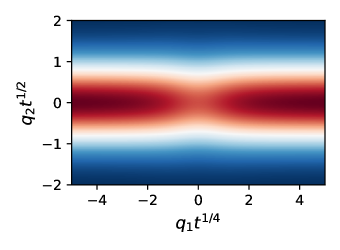
Figure 2: Scaling form assumed at large times $t$ by the intermediate scattering function $\mathfrak{F}(\mathbf{q},t)$ — see Section 4.4 and B for the details. The amplitude of the ISF is zero in correspondence of the dark blue regions, and maximum in correspondence of the red regions. The plot is obtained for a system of size $\mathcal{V}=100$ in $d=2$, where the combination $\mu(T+u_{\mathbf{q}=\bm{0}})$ and the maximum amplitude of the ISF were normalized to unity for illustrative purposes.

The stationary correlator in Eq. 58, obtained within the linearized SDFT, is one of the key results of this work: it encodes all dynamical correlations of the fluctuating particle density. Various dynamical observables, such as structure factors and first passage times, can be accessed starting from Eq. 58; as an application, here we consider the intermediate scattering function (ISF)

$$\mathfrak{F}(\mathbf{q},t)=\frac{1}{N}\expectationvalue{\rho_{\mathbf{q}}(t)\rho_{-\mathbf{q}}(0)}-\rho_{0}\delta^{d}(\mathbf{q})=\frac{\rho_{0}}{N}\expectationvalue{\phi_{\mathbf{q}}(t)\phi_{-\mathbf{q}}(0)}=\frac{\rho_{0}}{N}\mathcal{C}_{\mathbf{q},-\mathbf{q}}(t).$$ (59)

As we demonstrate in B, for sufficiently large times $t$ the ISF assumes a scaling form $\mathfrak{F}(q_{1}t^{\frac{1}{4}},q_{\perp}t^{\frac{1}{2}})$ that is independent of the specifics of the interaction potential $u(\mathbf{x})$, and which we compute explicitly for the case $d=2$ (see Eq. 176). The resulting scaling function is plotted in Fig. 2 for selected choices of the various parameters, and with its amplitude rescaled to unity for graphical convenience. Such ISF is manifestly reminiscent of the anisotropy of the comb structure.

4.5 Proof that the stationary and equilibrium correlators coincide

In the previous section we computed the equilibrium correlator, see Eq. 58. However, as we stressed under Eq. 14, there is no reason to believe a priori that the stationary state of the system is also an equilibrium one. To this end, here we prove that the solution obtained in Section 4.4 is unique — namely, that no other function exists for this system with the property of time-translational invariance required in Eq. 47.

We start by noting that an alternative and more direct way to impose the time-translational invariance $C_{\mathbf{q},\mathbf{p}}(t,t^{\prime})=\mathcal{C}_{\mathbf{q},\mathbf{p}}(t-t^{\prime})$ of the correlator (without invoking the fluctuation-dissipation theorem, which holds only at equilibrium) is to require

$$(\partial_{t}+\partial_{t^{\prime}})C_{\mathbf{q},\mathbf{p}}(t,t^{\prime})=0.$$ (60)

This condition can be used to construct the stationary correlator as follows. First, we change indices in the field equation (27) and write an evolution equation for $\partial_{t^{\prime}}\phi_{\mathbf{p}}(t^{\prime})$. Next, we multiply it by $\phi_{\mathbf{q}}(t)$ and take its average over the noise. This gives another Schwinger-Dyson equation,

$$\partial_{t^{\prime}}C_{\mathbf{q},\mathbf{p}}(t,t^{\prime})= -\mu p_{\perp}^{2}\,(T+u_{\mathbf{p}})C_{\mathbf{q},\mathbf{p}}(t,t^{\prime})-\mu p_{1}^{2}\,\int\frac{\differential[d-1]{{k}_{\perp}}}{(2\pi)^{d-1}}(T+u_{p_{1},-\mathbf{k}_{\perp}})C_{\mathbf{q},(p_{1},\mathbf{k}_{\perp})}(t,t^{\prime})$$

$$+R_{\mathbf{q},\mathbf{p}}(t,t^{\prime}),$$ (61)

akin to Eq. 39, which can then be summed to the latter. Setting the result equal to zero as per Eq. 60, and upon introducing

$$\mathcal{G}_{\mathbf{q},\mathbf{p}}^{-1}\equiv\mu\left[q_{\perp}^{2}\,(T+u_{\mathbf{q}})+p_{\perp}^{2}\,(T+u_{\mathbf{p}})\right],$$ (62)

$$S_{\mathbf{q},\mathbf{p}}(t,t^{\prime})\equiv R_{\mathbf{q},\mathbf{p}}(t,t^{\prime})+R_{\mathbf{p},\mathbf{q}}(t^{\prime},t),$$ (63)

we find

$$C_{\mathbf{q},\mathbf{p}}(t,t^{\prime})= \,\mathcal{G}_{\mathbf{q},\mathbf{p}}\,S_{\mathbf{q},\mathbf{p}}(t,t^{\prime})-\mu\mathcal{G}_{\mathbf{q},\mathbf{p}}\Bigg{[}q_{1}^{2}\,\int\frac{\differential[d-1]{{k}_{\perp}}}{(2\pi)^{d-1}}(T+u_{q_{1},-\mathbf{k}_{\perp}})C_{(q_{1},\mathbf{k}_{\perp}),\mathbf{p}}(t,t^{\prime})$$

$$+p_{1}^{2}\,\int\frac{\differential[d-1]{{k}_{\perp}}}{(2\pi)^{d-1}}(T+u_{p_{1},-\mathbf{k}_{\perp}})C_{\mathbf{q},(p_{1},\mathbf{k}_{\perp})}(t,t^{\prime})\Bigg{]}.$$ (64)

This integral equation is analyzed in A.5, were it is demonstrated that it admits a unique solution, corresponding to the equilibrium correlator found in Eq. 58.

5 Tracer particle dynamics

We now reinstate the coupling between the bath density and the tracer particle in Eqs. 17 and 16. The resulting coupled equations for the tracer and the bath density read, in Fourier space,

$$\dot{r}_{0}(t)=-h\mu_{0}\int\frac{\differential[d]{q}}{(2\pi)^{d}}iq_{1}v_{\mathbf{q}}\phi_{\mathbf{q}}(t)\mathrm{e}^{iq_{1}r_{0}(t)}+\eta_{0}(t),$$ (65)

with $\expectationvalue{\eta_{0}(t)\eta_{0}(t^{\prime})}=2\mu_{0}T\delta(t-t^{\prime})$, and

$$\partial_{t}\phi_{\mathbf{q}}(t)= \,-\mu q_{\perp}^{2}\,(T+u_{\mathbf{q}})\phi_{\mathbf{q}}(t)-\mu q_{1}^{2}\,\int\frac{\differential[d-1]{{p}_{\perp}}}{(2\pi)^{d-1}}(T+u_{q_{1},-\mathbf{p}_{\perp}})\phi_{q_{1},\mathbf{p}_{\perp}}(t)+\nu_{\mathbf{q}}(t)$$

$$-h\mu\left[q_{\perp}^{2}v_{\mathbf{q}}+q_{1}^{2}v_{q_{1}}(\mathbf{x}_{\perp}=\bm{0})\right]\mathrm{e}^{-iq_{1}r_{0}(t)},$$ (66)

with the correlations of $\nu_{\mathbf{q}}(t)$ given in Eq. 29. Above we denoted for brevity $h\equiv\rho_{0}^{-1/2}$.

With this in hands, in the next two sections we tackle two distinct (but related) problems using perturbation theory for small $h$:

1. In Section 5.1 we analyze the generalized correlation profiles between the tracer position and the density of surrounding bath particles [37].

2. In Section 5.2 we use such correlation profiles to access the effective tracer particle dynamics, and in particular its effective diffusion coefficient [36].

Note that, being constrained to move only along the backbone, the tracer particle will actually always exhibit diffusive behavior in spite of the comb geometry (whereas the other bath particles subdiffuse along the backbone).

5.1 Generalized correlation profiles

The simplest measure of the cross correlations between the tracer position and the density of surrounding bath particles is the average density profile in the reference frame of the tracer:

$$\psi(\mathbf{x},t)\equiv\expectationvalue{\phi(\mathbf{x}+\mathbf{r}_{0}(t),t)}\qquad\to\qquad\psi_{\mathbf{q}}(t)=\expectationvalue{\phi_{\mathbf{q}}(t)\mathrm{e}^{i\mathbf{q}\cdot\mathbf{r}_{0}(t)}},$$ (67)

where we called $\mathbf{r}_{0}(t)=r_{0}(t)\,\hat{\mathbf{e}}_{1}$. In the stationary state attained by the system at long times, this quantity can be evaluated by using Stratonovich calculus and the Novikov theorem, as delineated in C, resulting in

$$\psi_{\mathbf{q}} =-h\frac{v_{\mathbf{q}}}{T+u_{\mathbf{q}}}+\order{h^{2}}.$$ (68)

Crucially, this prediction is exactly the same as for homogeneous $d$-dimensional space, i.e. without the comb constraint [37]. Indeed, a non-perturbative calculation shows Eq. 68 to follow directly from the equilibrium distribution in Eq. 14, showing once again that the latter correctly represents the stationary state of the system.

However, signatures of the comb structure are expected to show up by considering higher-order correlation profiles such as

$$g(\mathbf{x},t)\equiv\expectationvalue{r_{0}(t)\phi(\mathbf{x}+\mathbf{r}_{0}(t),t)}\qquad\to\qquad g_{\mathbf{q}}(t)=\expectationvalue{r_{0}(t)\phi_{\mathbf{q}}(t)\mathrm{e}^{i\mathbf{q}\cdot\mathbf{r}_{0}(t)}}.$$ (69)

In particular, all correlations profiles of the form $\expectationvalue{[r_{0}(t)]^{n}\phi(\mathbf{x}+\mathbf{r}_{0}(t),t)}$ (for integer $n$) are compactly encoded in the generating function [46]

$$w(\mathbf{x},\lambda,t)\equiv\frac{\expectationvalue{\phi(\mathbf{x}+\mathbf{r}_{0}(t),t)\,\mathrm{e}^{\lambda\,r_{0}(t)}}}{\expectationvalue{\mathrm{e}^{\lambda\,r_{0}(t)}}}\qquad\to\qquad w_{\mathbf{q}}(\lambda,t)=\frac{\expectationvalue{\phi_{\mathbf{q}}(t)\mathrm{e}^{(\lambda+iq_{1})r_{0}(t)}}}{\expectationvalue{\mathrm{e}^{\lambda\,r_{0}(t)}}},$$ (70)

from which they can be retrieved by taking derivatives with respect to $\lambda$, before setting $\lambda=0$. Again, these quantities can be evaluated by using Stratonovich calculus and the Novikov theorem, as shown in C. In particular, the generating function reads in the stationary limit

$$w_{\mathbf{q}}(\lambda)=hG_{0}(\mathbf{q},\lambda)\Bigg{\{} \frac{v_{\mathbf{q}}}{T+u_{\mathbf{q}}}\left[i\mu_{0}Tq_{1}(\lambda+iq_{1})-\mu q_{\perp}^{2}(T+u_{\mathbf{q}})\right]$$

$$-\mu q_{1}^{2}\frac{v_{q_{1}}(\mathbf{x}_{\perp}=\bm{0})+M^{(4)}(q_{1},\lambda)}{1+\mu q_{1}^{2}M^{(3)}(q_{1},\lambda)}\Bigg{\}}+\order{h^{2}},$$ (71)

where

$$G_{0}^{-1}(\mathbf{q},\lambda) \equiv\mu q_{\perp}^{2}(T+u_{\mathbf{q}})-i\mu_{0}Tq_{1}(2\lambda+iq_{1}),$$ (72)

$$M^{(3)}(q_{1},\lambda) \equiv\int\frac{\differential[d-1]{{q}_{\perp}}}{(2\pi)^{d-1}}(T+u_{-\mathbf{q}})\,G_{0}(\mathbf{q},\lambda),$$ (73)

$$M^{(4)}(q_{1},\lambda) \equiv\int\frac{\differential[d-1]{{q}_{\perp}}}{(2\pi)^{d-1}}v_{\mathbf{q}}\,G_{0}(\mathbf{q},\lambda)\left[i\mu_{0}q_{1}T(\lambda+iq_{1})-\mu q_{\perp}^{2}(T+u_{\mathbf{q}})\right].$$ (74)

Similarly, the correlation profile $g_{\mathbf{q}}(t)$ introduced in Eq. 69 turns out to reduce in the stationary state to (see C)

$$g_{\mathbf{q}} =h\frac{i\mu_{0}Tq_{1}}{\mu q_{\perp}^{2}(T+u_{\mathbf{q}})+\mu_{0}Tq_{1}^{2}}\left[\frac{q_{1}^{2}M^{(2)}(q_{1})}{1+q_{1}^{2}M^{(1)}(q_{1})}-\frac{v_{\mathbf{q}}}{T+u_{\mathbf{q}}}\right]+\order{h^{2}},$$ (75)

where we called

$$M^{(1)}(q_{1}) \equiv\int\frac{\differential[d-1]{{q}_{\perp}}}{(2\pi)^{d-1}}\frac{\mu(T+u_{-\mathbf{q}})}{\mu q_{\perp}^{2}(T+u_{\mathbf{q}})+\mu_{0}Tq_{1}^{2}},$$ (76)

$$M^{(2)}(q_{1}) \equiv\int\frac{\differential[d-1]{{q}_{\perp}}}{(2\pi)^{d-1}}\frac{\mu v_{\mathbf{q}}}{\mu q_{\perp}^{2}(T+u_{\mathbf{q}})+\mu_{0}Tq_{1}^{2}}.$$ (77)

By symmetry in the momenta $\mathbf{q}$, we deduce that $g(-\mathbf{x})=-g(\mathbf{x})$, as expected from its definition (69) — see also the inset of Fig. 3(a). Moreover, if $\mu_{0}=\mu$, then the stationary correlation profile $g_{\mathbf{q}}$ becomes independent of the particle mobility. In $d=2$ and setting $v_{\mathbf{q}}=u_{\mathbf{q}}$, it is then simple to derive its large-distance behavior (see C)

$$g(x_{1})\sim\frac{h\sqrt{T}u_{\mathbf{q}=\bm{0}}}{2\pi(T+u_{\mathbf{q}=\bm{0}})^{3/2}}x_{1}^{-1}.$$ (78)

This asymptotic behavior is checked in Fig. 3(a). Remarkably, it is consistent with the behavior $g(x_{1})\sim x_{1}^{1-d}$ observed in uniform $d$-dimensional space (i.e. without the comb) in Ref. [37], for a wide class of interacting particle systems ranging from hard-core lattice models, to Lennard-Jones fluids. The claim of universality of the large-distance behavior of the correlation profile $g(\mathbf{x})$, put forward in [37], is thus further validated by Eq. 78.

5.2 Effective diffusion coefficient

In this Section we focus on the effective dynamics of the tracer particle, and we derive the first perturbative correction to its diffusion coefficient, due to the presence of the other bath particles. First, note that the leading-order correction to the generalized profiles computed in Section 5.1 turned out to be of $\order{h}$. Conversely, any correlation function involving $\mathbf{r}$ but not $\phi$ must exhibit corrections at least of $\order{h^{2}}$ — the simplest way to prove this fact is to note that the system of equations (65)–(66) is invariant under the transformation $\{h\mapsto-h,\phi\mapsto-\phi\}$ [47, 39]. In general, the perturbative calculation of the effective diffusion coefficient in homogeneous space can be compactly addressed within the path-integral formalism developed in Ref. [38] (and later adopted in e.g. Refs. [36, 48]). However, it is not evident how to extend such path-integral techniques to the case of non-homogeneous space analyzed here. By contrast, we showed in Ref. [37] that the bath-tracer correlation profiles — that we already derived in the previous Section — actually encode the tracer statistics, and thus offer a straightforward alternative way to access its diffusion coefficient.

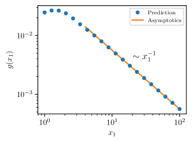
Figure 3: (a) Tracer-bath spatial correlation profile $g(x_{1})$, whose Fourier transform is predicted by Eq. 75 in the long-time stationary state. Its asymptotic scale-free behavior is given in Eq. 78, while the inset shows its symmetry $g(-\mathbf{x})=-g(\mathbf{x})$. In the plot we chose a Gaussian interaction potential $u_{\mathbf{q}}=\exp(-q^{2}/2)$, and we set $h$ and $T$ to unity for simplicity. (b) Comparison between the effective diffusion coefficient $D_{\text{eff}}$ predicted by Eq. 89, and the results of numerical simulations of a system of particles interacting via Gaussian potentials of strength $\epsilon$. In the plot, we vary $\epsilon$ (and hence the dimensionless parameter $\theta_{1}\equiv\epsilon\rho_{0}\sigma^{d}/T$, see Section 5.2), with all other parameters kept fixed. Details of the numerical simulation are reported in D.

To show this, let us focus on the moment generating function

$$\varphi(q_{1},t)\equiv\expectationvalue{\mathrm{e}^{-iq_{1}r_{0}(t)}},$$ (79)

that we aim to compute in the stationary regime. To this end, one can first use Stratonovich calculus to derive, starting from Eqs. 65 and 66, the relation

$$\partial_{t}\expectationvalue{\mathrm{e}^{\lambda\,r_{0}(t)}}=\lambda\expectationvalue{\eta(t)\mathrm{e}^{\lambda\,r_{0}(t)}}-h\mu_{0}\lambda\cdot\int\frac{\differential[d]{p}}{(2\pi)^{d}}ip_{1}v_{\mathbf{p}}\expectationvalue{\mathrm{e}^{(\lambda+ip_{1})r_{0}(t)}\phi_{\mathbf{p}}(t)}.$$ (80)

The second expectation value on the r.h.s. of Eq. 80 is reminiscent of a quantity we have already met, i.e. $w_{\mathbf{p}}(\lambda,t)$ introduced in Eq. 70. Since the evolution equation for $w_{\mathbf{p}}(\lambda,t)$ (derived perturbatively in C.1) admits as a stationary solution $w_{\mathbf{p}}(\lambda)$ given in Eq. 70, here it is reasonable to assume that

$$\expectationvalue{\mathrm{e}^{(\lambda+ip_{1})r_{0}(t)}\phi_{\mathbf{p}}(t)}=w_{\mathbf{p}}(\lambda,t)\expectationvalue{\mathrm{e}^{\lambda\,r_{0}(t)}}\simeq w_{\mathbf{p}}(\lambda)\expectationvalue{\mathrm{e}^{\lambda\,r_{0}(t)}},$$ (81)

in the stationary regime. Plugging this into Eq. 80 then gives

$$\partial_{t}\expectationvalue{\mathrm{e}^{\lambda\,r_{0}(t)}}=\lambda\expectationvalue{\eta(t)\mathrm{e}^{\lambda\,r_{0}(t)}}-h\mu_{0}\expectationvalue{\mathrm{e}^{\lambda\,r_{0}(t)}}\lambda_{1}\int\frac{\differential[d]{p}}{(2\pi)^{d}}ip_{1}v_{\mathbf{p}}w_{\mathbf{p}}(\lambda).$$ (82)

On the other hand, the first expectation value on the r.h.s. of Eqs. 80 and 82 can be computed by standard methods using the Novikov theorem [49], and the result reads

$$\expectationvalue{\eta(t)\mathrm{e}^{\lambda\,r_{0}(t)}}=\mu_{0}T\lambda\expectationvalue{\mathrm{e}^{\lambda\,r_{0}(t)}},$$ (83)

which is the same as for a non-interacting tracer (in spite of the interaction with the bath density, see Ref. [37] for further details). By setting $\lambda=-iq_{1}$ and using Eq. 79, we thus obtain

$$\partial_{t}\varphi(q_{1},t)=-q_{1}^{2}\mu_{0}T\varphi(q_{1},t)-h\mu_{0}\varphi(q_{1},t)\int\frac{\differential[d]{p}}{(2\pi)^{d}}(p_{1}\cdot q_{1})v_{\mathbf{p}}w_{\mathbf{p}}(-iq_{1}),$$ (84)

whose solution

$$\ln\varphi(q_{1},t)=-\mu_{0}t\left[q_{1}^{2}T+h\int\frac{\differential[d]{p}}{(2\pi)^{d}}(p_{1}\cdot q_{1})v_{\mathbf{p}}w_{\mathbf{p}}(-iq_{1})\right]$$ (85)

gives the leading-order correction to the cumulant generating function of the tracer position, and can be made explicit upon using the leading-order estimate of $w_{\mathbf{p}}(\lambda)$ found in Eq. 71. First, we note that $\mathbf{r}_{0}(t)$ has non-Gaussian statistics. In particular, one can check that $\varphi(q_{1}=0,t)=1$ and

$$\expectationvalue{r_{0}(t)}=\evaluated{i\frac{\partial\varphi(q_{1},t)}{\partial q_{1}}}_{q_{1}=0}=0,$$ (86)

as expected, while the variance reads

$$\expectationvalue{r_{0}^{2}(t)} =\evaluated{-\frac{\partial^{2}}{\partial q_{1}^{2}}\varphi(q_{1},t)}_{q_{1}=0}$$ (87)

$$=2\mu_{0}Tt\left\{1-h^{2}\int\frac{\differential{p_{1}}}{2\pi}p_{1}^{2}\left[M^{(5)}(p_{1})-\frac{\mu_{0}}{\mu}\frac{[p_{1}M^{(2)}(p_{1})]^{2}}{1+p_{1}^{2}M^{(1)}(p_{1})}\right]\right\}+\order{h^{4}},$$

where

$$M^{(5)}(p_{1})\equiv\int\frac{\differential[d-1]{{p}_{\perp}}}{(2\pi)^{d-1}}\frac{\mu_{0}v_{\mathbf{p}}^{2}}{(T+u_{\mathbf{p}})[\mu q_{\perp}^{2}(T+u_{\mathbf{q}})+\mu_{0}Tq_{1}^{2}]},$$ (88)

while the functions $M^{(1,2)}(p_{1})$ were given in Eqs. 76 and 77, respectively. Calling $D_{0}=\mu T$ the bare diffusion coefficient of the non-interacting tracer, from Eq. 87 we thus obtain $\expectationvalue{r_{0}^{2}(t)}=2D_{\text{eff}}t$ with the effective diffusion coefficient

$$\frac{D_{\text{eff}}}{D_{0}}=1-h^{2}\int\frac{\differential{p_{1}}}{2\pi}p_{1}^{2}\left[M^{(5)}(p_{1})-\frac{\mu_{0}}{\mu}\frac{[p_{1}M^{(2)}(p_{1})]^{2}}{1+p_{1}^{2}M^{(1)}(p_{1})}\right]+\order{h^{4}}.$$ (89)

This prediction represents another key result of this work, and is the spatially heterogeneous counterpart to the diffusion coefficient first obtained in Refs. [38, 36] for homogeneous media, using path-integral methods.

Note that Eq. 85 apparently implies that all other higher-order cumulants of $r_{0}(t)$ also grow linearly with $t$. However, we stress that Eq. 85 has been derived under the assumption that $w_{\mathbf{q}}(\lambda,t)$ becomes stationary, and must thus be taken with caution — we comment further on this point in C.3.

Again, we note that for $\mu_{0}=\mu$ the second term in Eq. 89 actually becomes $\mu$-independent. To be concrete, we now set $v_{\mathbf{q}}=u_{\mathbf{q}}$, and assume for the interaction potential in real space $U(\mathbf{x})$ the general rotationally invariant form

$$U(\mathbf{x})=\epsilon f(x/\sigma),$$ (90)

where $x=\absolutevalue{\mathbf{x}}$, $\epsilon$ is an energy scale, $\sigma$ is a microscopic length scale, and the function $f$ is dimensionless. For example, within the Gaussian core model one has $U(x)=\epsilon\exp[-x^{2}/(2\sigma^{2})]$. In Fourier space, the corresponding rescaled interaction potential $u_{\mathbf{q}}=\rho_{0}U_{\mathbf{q}}$ then reads

$$u_{\mathbf{q}}=\rho_{0}\epsilon\,\sigma^{d}f(q\sigma).$$ (91)

By inspecting Eq. 89 with $\mu_{0}=\mu$, and upon reinstating the microscopic length scale $a$ by replacing $q_{1}^{2}\mapsto a^{d-1}q_{1}^{2}$ (see the discussion under Eq. 6), it is then simple to see that $D_{\text{eff}}/D_{0}$ only depends on the dimensionless combinations $\theta_{1}\equiv\epsilon\rho_{0}\sigma^{d}/T$, $\theta_{2}=\rho_{0}\sigma^{d}$, and $\theta_{3}=R/a$, rather than on these parameters taken separately. In Fig. 3(b) we thus compare our prediction in Eq. 89 to the results of numerical simulations obtained by varying the interaction strength $\epsilon$ with all other parameters fixed (see D for the details), which amounts to varying the effective parameter $\theta_{1}$. The prediction is shown to be accurate for small interaction strengths $\epsilon\ll k_{B}T$, as usually expected within the linearized Dean-Kawasaki theory [36, 37].

6 Conclusions

In this work we considered a system of overdamped Brownian particles interacting via soft pairwise potentials, and constrained to move on a comb-like structure (see Fig. 1). Within the Dean-Kawasaki formalism, we first derived in Section 3 the exact coarse-grained equations that describe the dynamics of the particle density field $\rho(\mathbf{x},t)$. The latter can be expanded around a uniform background density, which allowed us to characterize the Gaussian fluctuations of the density field. In particular, in Section 4 we computed the density-density correlator both starting from fixed initial conditions (see Eq. 44), and in the stationary limit assumed by the system at long times (see Eq. 58). The latter can be used to construct for instance the intermediate scattering function shown in Fig. 2. To the best of our knowledge, this represents the first application of the Dean-Kawasaki theory to non-homogeneous media [34, 35].

Furthermore, in Section 5 we singled out a tagged tracer from the bath of interacting particles, under the assumption that it is constrained to move only along the backbone. In this setting, we derived the spatial correlation profile between the tracer position and the surrounding bath density (see Eq. 75 and Fig. 3(a)), and the effective diffusion coefficient of the tracer, which we tested using Brownian dynamics simulations (see Eq. 89 and Fig. 3(b)).

Further extensions of this work could address the unconstrained problem in which the tracer particle is allowed to leave the backbone (which is technically more challenging than the constrained case considered in this work, even within the perturbation theory delineated in Section 5). This would ideally provide access to the effective subdiffusion coefficient of the tracer along the backbone, i.e. to its correction due to the presence of the other bath particles. Moreover, the framework delineated in Section 3 can in principle be extended to other non-homogeneous geometries, which can be encoded with a suitable choice of the particle’s mobility matrix $\hat{\mu}(\mathbf{x})$ in Eq. 1.

Appendix A Details on the dynamics of the density fluctuations

In this Appendix we completely characterize the density fluctuations on the comb by deriving the results reported in Section 4. In particular, in A.1, A.2, and A.3 we provide the derivations of the propagator, response function, and Dirichlet correlator, respectively. In A.4 we then derive the stationary correlator, proving in A.5 that it coincides with the equilibrium correlator (in spite of the geometrical constraints of the system, which could in principle preclude ergodicity). In A.6 we recall a few causality properties of the double Laplace transform, and finally in A.7 we analyze the free (Gaussian) field [45], as a test bench for the techniques employed on the comb.

A.1 Derivation of the propagator

We start from Eq. 31, which rules the evolution of the Fourier transform $G_{\mathbf{q}}(t)$ of the propagator $G(\mathbf{x},t)$. We then Laplace-transform the last equation: using that $G(\mathbf{x},t=0^{+})=0$ by construction, we find

$$G_{\mathbf{q}}(s)=g_{\perp}(\mathbf{q}_{\perp},s)\left[1-\mu q_{1}^{2}F(q_{1},s)\right],$$ (92)

where $g_{\perp}$ was defined in Eq. 33, while we introduced the auxiliary function

$$F(q_{1},s)=\int\frac{\differential[d-1]{{q}_{\perp}}}{(2\pi)^{d-1}}(T+u_{q_{1},-\mathbf{q}_{\perp}})G_{\mathbf{q}}(s).$$ (93)

Crucially, the terms enclosed in square brackets in Eq. 92 do not depend on $\mathbf{q}_{\perp}$. Upon applying $\int\frac{\differential[d-1]{{q}_{\perp}}}{(2\pi)^{d-1}}(T+u_{q_{1},-\mathbf{q}_{\perp}})$ to Eq. 92, we thus obtain the self-consistent equation

$$F(q_{1},s)=M(q_{1},s)\left[1-\mu q_{1}^{2}F(q_{1},s)\right],$$ (94)

where we introduced the function

$$M(q_{1},s)=\int\frac{\differential[d-1]{{q}_{\perp}}}{(2\pi)^{d-1}}(T+u_{q_{1},-\mathbf{q}_{\perp}})g_{\perp}(\mathbf{q}_{\perp},s).$$ (95)

We thus solve Eq. 94 to obtain $F$, which can then be replaced into Eq. 92 to give

$$G_{\mathbf{q}}(s)=\frac{g_{\perp}(\mathbf{q}_{\perp},s)}{1+\mu q_{1}^{2}M(q_{1},s)}.$$ (96)

Upon calling (compare with Eq. 34)

$$g_{1}^{-1}(q_{1},s)\equiv 1+\mu q_{1}^{2}M(q_{1},s)$$ (97)

the denominator in Eq. 96, we obtain the expression of $G_{\mathbf{q}}(s)$ reported in Eq. 32.

Note that Eq. 31 reduces, for $u_{\mathbf{q}}=0$ and in $d=2$, to the Fourier transform of the Fokker-Planck equation (7) for a single (non-interacting) Brownian particle on the comb, placed initially at the origin at time $t=0$. The corresponding $G_{\mathbf{q}}(s)$, i.e. its moment generating function written in the Laplace domain, then reduces to

$$G_{\mathbf{q}}(s)=(s+\mu Tq_{2}^{2})^{-1}\left[1+\frac{a\sqrt{\mu T}q_{1}^{2}}{2\sqrt{s}}\right]^{-1},$$ (98)

where we computed explicitly the integral in the definition (34) of $g_{1}(q_{1},s)$, and we reinstated the length scale $q_{1}^{2}\mapsto aq_{1}^{2}$ (see the discussion under Eq. 6). In particular, one can use Tauberian theorems [50] to deduce the long-$t$ behavior of the inverse Laplace transform of the particle variance along the two orthogonal directions:

$$-\evaluated{\partialderivative[2]{G_{\mathbf{q}}(s)}{q_{2}}}_{\mathbf{q}=\bm{0}}=2\mu Ts^{-2}\qquad\leftrightarrow\qquad\expectationvalue{y^{2}(t)}\simeq 2\mu Tt,$$ (99)

and

$$-\evaluated{\partialderivative[2]{G_{\mathbf{q}}(s)}{q_{1}}}_{\mathbf{q}=\bm{0}}=a\sqrt{\mu T}s^{-\frac{3}{2}}\qquad\leftrightarrow\qquad\expectationvalue{x^{2}(t)}\simeq 2a\sqrt{\frac{\mu Tt}{\pi}}.$$ (100)

Alternatively, one can invert explicitly Eq. 98 to the time domain, finding

$$G_{\mathbf{q}}(t)=\frac{4q_{2}^{2}\mathrm{e}^{-q_{2}^{2}\mu Tt}-4aq_{1}^{2}\sqrt{\frac{q_{2}^{2}}{\pi}}\,\mathrm{DawsonF}\left(\sqrt{q_{2}^{2}\mu Tt}\right)+a^{2}\mathrm{e}^{\frac{q_{1}^{4}}{4}a^{2}\mu Tt}q_{1}^{4}\,\mathrm{Erfc}\left(\frac{q_{1}^{2}}{2}a\sqrt{\mu Tt}\right)}{a^{2}q_{1}^{4}+4q_{2}^{2}},$$ (101)

which leads to the same asymptotics in the long-$t$ limit.

A.2 Derivation of the response function

We start by Laplace transforming the corresponding Schwinger-Dyson equation (40) with respect to both $t\rightarrow s$ and $t^{\prime}\rightarrow s^{\prime}$, finding

$$sR_{\mathbf{q},\mathbf{p}}(s,s^{\prime})= -\mu q_{\perp}^{2}\,(T+u_{\mathbf{q}})R_{\mathbf{q},\mathbf{p}}(s,s^{\prime})-\mu q_{1}^{2}\,\int\frac{\differential[d-1]{{k}_{\perp}}}{(2\pi)^{d-1}}(T+u_{q_{1},-\mathbf{k}_{\perp}})R_{(q_{1},\mathbf{k}_{\perp}),\mathbf{p}}(s,s^{\prime})$$

$$+\frac{2\mu T}{s+s^{\prime}}\left[q_{1}^{2}\delta(q_{1}+p_{1})+q_{\perp}^{2}\delta^{d}(\mathbf{q}+\mathbf{p})\right].$$ (102)

Note that the first Laplace transform, $t\rightarrow s$, acts on the first term in Eq. 40 as

$$\partial_{t}R_{\mathbf{q},\mathbf{p}}(t,t^{\prime})\qquad\rightarrow\qquad sR_{\mathbf{q},\mathbf{p}}(s,t^{\prime})-R_{\mathbf{q},\mathbf{p}}(t=0^{+},t^{\prime})\Theta(-t^{\prime}),$$ (103)

where the $\Theta(-t^{\prime})$ stems from the causality of the response function — see its definition in Eq. 38. The second Laplace transform, $t^{\prime}\rightarrow s^{\prime}$, then suppresses the term proportional to $\Theta(-t^{\prime})$.

Equation (102) can be rewritten as

$$R_{\mathbf{q},\mathbf{p}}(s,s^{\prime})=g_{\perp}(\mathbf{q},s)\left\{\frac{2\mu T}{s+s^{\prime}}\left[q_{1}^{2}\delta(q_{1}+p_{1})+q_{\perp}^{2}\delta^{d}(\mathbf{q}+\mathbf{p})\right]-\mu q_{1}^{2}F^{(1)}(q_{1};s,s^{\prime})\right\},$$ (104)

where we introduced the auxiliary function

$$F^{(1)}(q_{1};s,s^{\prime})\equiv\int\frac{\differential[d-1]{{q}_{\perp}}}{(2\pi)^{d-1}}(T+u_{q_{1},-\mathbf{q}_{\perp}})R_{\mathbf{q},\mathbf{p}}(s,s^{\prime}).$$ (105)

Applying the operator $\int\frac{\differential[d-1]{{q}_{\perp}}}{(2\pi)^{d-1}}(T+u_{q_{1},-\mathbf{q}_{\perp}})$ to Eq. 104 we thus obtain the self-consistency relation

$$F^{(1)}(q_{1};s,s^{\prime})= M(q_{1},s)\left[\frac{2\mu T}{s+s^{\prime}}q_{\perp}^{2}\delta^{d}(\mathbf{q}+\mathbf{p})-\mu q_{1}^{2}F^{(1)}(q_{1};s,s^{\prime})\right]$$

$$+\frac{2\mu T}{s+s^{\prime}}q_{1}^{2}\delta(q_{1}+p_{1})(T+u_{\mathbf{p}})g_{\perp}(-\mathbf{p},s).$$ (106)

From now on, we will assume for simplicity $u(\mathbf{x})$ to be rotationally invariant, so that $u_{\mathbf{q}}$ depends only on $\absolutevalue{\mathbf{q}}=q_{1}^{2}+q_{\perp}^{2}$. This implies in particular

$$g_{\perp}(\mathbf{q},s)=g_{\perp}(-\mathbf{q},s),\qquad M(q_{1},s)=M(-q_{1},s),$$ (107)

as it can easily be evinced from their definitions in Eqs. 33 and 95. Solving for $F^{(1)}$ in Eq. 106 and replacing the result into Eq. 104 then renders the response function given in Eq. 41, upon noting that

$$1-\mu p_{\perp}^{2}(T+u_{\mathbf{p}})g_{\perp}(\mathbf{p},s)=s\,g_{\perp}(\mathbf{p},s),$$ (108)

and by using the propagator $G_{\mathbf{q}}(s)$ introduced in Eq. 32.

Using the causality structure of the response function (see c.f. A.6), we can finally invert Eq. 41 with $u(\mathbf{x})=A\delta(\mathbf{x})$ and $d=2$, which gives

$$R_{\mathbf{q},\mathbf{p}}(t,t^{\prime})= \,\frac{2\mu T\Theta(\tau)q_{1}^{2}\delta(q_{1}+p_{1})}{(q_{2}^{2}-p_{2}^{2})(4p_{2}^{2}+p_{1}^{4})(4q_{2}^{2}+q_{1}^{4})}\Bigg{\{}2q_{2}^{3}(4p_{2}^{2}+p_{1}^{4})\mathrm{e}^{-q_{2}^{2}\mu\mathcal{T}\tau}\Big{[}2q_{2}$$

$$-q_{1}^{2}\text{Erfi}\left(q_{2}\sqrt{\mu\mathcal{T}\tau}\right)\Big{]}-(\mathbf{p}\leftrightarrow\mathbf{q})+\mathrm{e}^{\frac{q_{1}^{4}}{4}\mu\mathcal{T}\tau}(q_{2}^{2}-p_{2}^{2})q_{1}^{8}\text{Erfc}\left(\frac{q_{1}^{2}}{2}\sqrt{\mu\mathcal{T}\tau}\right)\Bigg{\}}$$

$$+2\mu T\Theta(\tau)p_{2}^{2}\delta(\mathbf{q}+\mathbf{p})\mathrm{e}^{-q_{2}^{2}\mu\mathcal{T}\tau},$$ (109)

with $\tau=t-t^{\prime}>0$ and $\mathcal{T}\equiv T+A$.

A.3 Derivation of the correlator for Dirichlet initial conditions

As in the previous sections, we start by Laplace-transforming the corresponding Schwinger-Dyson equation (39) with respect to $t\rightarrow s$, finding

$$C_{\mathbf{q},\mathbf{p}}(s,t^{\prime})= \,g_{\perp}(\mathbf{q},s)\Big{[}C_{\mathbf{q},\mathbf{p}}(t=0^{+},t^{\prime})-\mu q_{1}^{2}\,\int\frac{\differential[d-1]{{k}_{\perp}}}{(2\pi)^{d-1}}(T+u_{q_{1},-\mathbf{k}_{\perp}})C_{(q_{1},\mathbf{k}_{\perp}),\mathbf{p}}(s,t^{\prime})$$

$$+R_{\mathbf{p},\mathbf{q}}(t^{\prime},s)\Big{]}.$$ (110)

Note that this time the quantity $C_{\mathbf{q},\mathbf{p}}(t=0^{+},t^{\prime})\neq 0$. On the contrary, this term can be used to enforce any particular initial condition at $t_{0}=0$, because by construction

$$C_{\mathbf{q},\mathbf{p}}(t=t_{0},t^{\prime})=\phi_{\mathbf{q}}(t_{0})\phi_{\mathbf{p}}(t_{0})G_{\mathbf{p}}(t^{\prime}-t_{0}),$$ (111)

where $G_{\mathbf{q}}(t)$ is the propagator in Eq. 32. We remark that the seemingly arbitrary choice $t_{0}=0$ is necessary to allow the use of the Laplace transform, but in fact it entails no loss of generality. Indeed, once a particular solution $C_{\mathbf{q},\mathbf{p}}(t,t^{\prime})$ is found, one can simply introduce the new coordinates

$$\tau=t+t_{0},\qquad\tau^{\prime}=t^{\prime}+t_{0},$$ (112)

which practically amounts to shifting the initial conditions to the time $\tau=t_{0}$. In particular, this may allow to find the correlator in the stationary state by eventually taking the limit $t_{0}\to-\infty$.

Upon further Laplace-transforming Eq. 110 with respect to $t^{\prime}\to s^{\prime}$, we thus obtain

$$C_{\mathbf{q},\mathbf{p}}(s,s^{\prime})= \,g_{\perp}(\mathbf{q},s)\Big{[}\phi_{\mathbf{q}}^{(0)}\phi_{\mathbf{p}}^{(0)}G_{\mathbf{p}}(s^{\prime})-\mu q_{1}^{2}\,\int\frac{\differential[d-1]{{k}_{\perp}}}{(2\pi)^{d-1}}(T+u_{q_{1},-\mathbf{k}_{\perp}})C_{(q_{1},\mathbf{k}_{\perp}),\mathbf{p}}(s,s^{\prime})$$

$$+R_{\mathbf{p},\mathbf{q}}(s^{\prime},s)\Big{]},$$ (113)

where we called for brevity $\phi_{\mathbf{q}}^{(0)}\equiv\phi_{\mathbf{q}}(t=0)$, and where the response function $R_{\mathbf{q},\mathbf{p}}(s,s^{\prime})$ was given in Eq. 41 (note, however, the exchange of its arguments). Again, our strategy consists in integrating Eq. 113 with respect to $\mathbf{q}_{\perp}$ to obtain a self-consistency equation. To this end, we first collect the various term in Eq. 113 according to their dependence on $\mathbf{q}_{\perp}$, and use the property

$$g_{\perp}(\mathbf{q},s)g_{\perp}(\mathbf{q},s^{\prime})=\frac{g_{\perp}(\mathbf{q},s)-g_{\perp}(\mathbf{q},s^{\prime})}{s^{\prime}-s},$$ (114)

which is readily proven by inspection of the definition (33) of $g_{\perp}(\mathbf{q},s)$. We can thus rewrite

$$C_{\mathbf{q},\mathbf{p}}(s,s^{\prime})= \,g_{\perp}(\mathbf{q},s)\phi_{\mathbf{q}}^{(0)}\phi_{\mathbf{p}}^{(0)}G_{\mathbf{p}}(s^{\prime})+g_{\perp}(\mathbf{q},s)g_{\perp}(\mathbf{q},s^{\prime})\delta^{d}(\mathbf{q}+\mathbf{p})\frac{2\mu T}{s+s^{\prime}}p_{\perp}^{2}$$

$$+g_{\perp}(\mathbf{q},s)\left[\frac{2\mu T}{s+s^{\prime}}\frac{p_{1}^{2}\delta(q_{1}+p_{1})\,s^{\prime}\,G_{\mathbf{p}}(s^{\prime})}{s^{\prime}-s}-\mu q_{1}^{2}\,F^{(2)}(q_{1};s,s^{\prime})\right]$$

$$-g_{\perp}(\mathbf{q},s^{\prime})\frac{2\mu T}{s+s^{\prime}}\frac{p_{1}^{2}\delta(q_{1}+p_{1})\,s^{\prime}\,G_{\mathbf{p}}(s^{\prime})}{s^{\prime}-s},$$ (115)

where we introduced the auxiliary function

$$F^{(2)}(q_{1};s,s^{\prime})\equiv\int\frac{\differential[d-1]{{q}_{\perp}}}{(2\pi)^{d-1}}(T+u_{q_{1},-\mathbf{q}_{\perp}})C_{\mathbf{q},\mathbf{p}}(s,s^{\prime}).$$ (116)

Applying $\int\frac{\differential[d-1]{{q}_{\perp}}}{(2\pi)^{d-1}}(T+u_{q_{1},-\mathbf{q}_{\perp}})$ to Eq. 113 renders

$$F^{(2)}(q_{1};s,s^{\prime})= \,\phi_{\mathbf{p}}^{(0)}G_{\mathbf{p}}(s^{\prime})M^{(0)}(q_{1},s)+M(q_{1},s)\left[\mathcal{A}-\mu q_{1}^{2}\,F^{(2)}(q_{1};s,s^{\prime})\right]$$

$$-\mathcal{A}M(q_{1},s)+g_{\perp}(\mathbf{p},s)g_{\perp}(\mathbf{p},s^{\prime})\delta(q_{1}+p_{1})\frac{2\mu T}{s+s^{\prime}}p_{\perp}^{2}\,(T+u_{\mathbf{p}}),$$ (117)

where the functions $M^{(0)},M$ were introduced in Eqs. 95 and 45, respectively, and where we called for brevity

$$\mathcal{A}\equiv\frac{2\mu T}{s+s^{\prime}}\frac{p_{1}^{2}\delta(q_{1}+p_{1})\,s^{\prime}\,G_{\mathbf{p}}(s^{\prime})}{s^{\prime}-s}.$$ (118)

Solving for $F^{(2)}$ in Eq. 117 gives

$$\frac{F^{(2)}(q_{1};s,s^{\prime})}{g_{1}(q_{1},s)}= \,\phi_{\mathbf{p}}^{(0)}G_{\mathbf{p}}(s^{\prime})M^{(0)}(q_{1},s)+\mathcal{A}\left[M(q_{1},s)-M(q_{1},s^{\prime})\right]$$

$$+g_{\perp}(\mathbf{p},s)g_{\perp}(\mathbf{p},s^{\prime})\delta(q_{1}+p_{1})\frac{2\mu T}{s+s^{\prime}}p_{\perp}^{2}\,(T+u_{\mathbf{p}}),$$ (119)

which can be further simplified by rewriting

$$\mu p_{\perp}^{2}\,(T+u_{\mathbf{p}})=g^{-1}_{\perp}(\mathbf{p},s)-s,$$ (120)

$$\mu q_{1}^{2}\,\left[M(q_{1},s)-M(q_{1},s^{\prime})\right]=g^{-1}_{1}(q_{1},s)-g^{-1}_{1}(q_{1},s^{\prime}),$$ (121)

as one can easily check starting from the definitions of $g_{\perp},\,g_{1}$, and $M$ given in Eqs. 33, 34 and 95, respectively. Replacing the expression of $F^{(2)}$ found in Eq. 119 back into Eq. 115 renders, after some algebra, the correlation function $C_{\mathbf{q},\mathbf{p}}(s,s^{\prime})$ reported in Eq. 44.

Note that specializing the latter to flat initial conditions $\phi_{\mathbf{q}}^{(0)}\mapsto\phi^{(0)}$ yields

$$\phi_{\mathbf{p}}^{(0)}G_{\mathbf{p}}(s^{\prime})g_{\perp}(\mathbf{q},s)\left[\phi_{\mathbf{q}}^{(0)}-\mu q_{1}^{2}g_{1}(q_{1},s)M^{(0)}(q_{1},s)\right]$$

$$\mapsto\left[\phi^{(0)}\right]^{2}G_{\mathbf{p}}(s^{\prime})g_{\perp}(\mathbf{q},s)\left[1-\mu q_{1}^{2}g_{1}(q_{1},s)M(q_{1},s)\right]=\left[\phi^{(0)}\right]^{2}G_{\mathbf{q}}(s)G_{\mathbf{p}}(s^{\prime}),$$ (122)

where the second step follows from the definitions of $M^{(0)},M$ given in Eqs. 95 and 45, while in the third step we recognized

$$1-\mu q_{1}^{2}\,g_{1}(q_{1},s)M(q_{1},s)=g_{1}(q_{1},s),$$ (123)

and we used the definition (32) of $G_{\mathbf{q}}(s)$.

A.4 Derivation of the equilibrium correlator

First, we note that simpler field theories generally allow to find the stationary correlator starting from the Dirichlet correlator computed in correspondence of fixed initial conditions at time $t=t_{0}$. Indeed, if a time-domain expression of $C_{\mathbf{q},\mathbf{p}}(t,t^{\prime})$ is available, one can formally send $t_{0}\to-\infty$, as we remarked at the beginning of A.3. We exemplify this route in A.7 for the simple case of the free (Gaussian) field [45]. However, directly inverting the Laplace expression of $C_{\mathbf{q},\mathbf{p}}(s,s^{\prime})$ found in Eq. 44 proved challenging in the present context.

The strategy we adopt in this Section hinges instead on the assumption that the system reaches at long times the equilibrium distribution given in Eq. 56. Here the fluctuation-dissipation theorem (in the form of Eq. 54) links the stationary correlator $\mathcal{C}_{\mathbf{q},\mathbf{p}}(\tau)$ to the linear susceptibility

$$\chi_{\mathbf{q},\mathbf{p}}(t,t^{\prime})\equiv\evaluated{\functionalderivative{\expectationvalue{\phi_{\mathbf{q}}(t)}}{j_{-\mathbf{p}}(t^{\prime})}}_{j=0},$$ (124)

computed in the presence of a field $j(\mathbf{x},t)$ linearly coupled to the Hamiltonian as in Eq. 50. The corresponding equation of motion follows from Eq. 25 as

$$\partial_{t}\phi(\mathbf{x},t)=\divergence\left\{\hat{\mu}(\mathbf{x})\gradient\left[T\phi(\mathbf{x},t)+\int\differential{\mathbf{y}}u(\mathbf{x}-\mathbf{y})\phi(\mathbf{y})-j(\mathbf{x},t)\right]+\bm{\xi}(\mathbf{x},t)\right\}.$$ (125)

Taking its average, its spatial Fourier transform, and finally its functional derivative as in Eq. 124, leads to the following evolution equation for the susceptibility:

$$\partial_{t}\chi_{\mathbf{q},\mathbf{p}}(t,t^{\prime})= -\mu q_{\perp}^{2}\,(T+u_{\mathbf{q}})\chi_{\mathbf{q},\mathbf{p}}(t,t^{\prime})-\mu q_{1}^{2}\,\int\frac{\differential[d-1]{{k}_{\perp}}}{(2\pi)^{d-1}}(T+u_{q_{1},-\mathbf{k}_{\perp}})\chi_{(q_{1},\mathbf{k}_{\perp}),\mathbf{p}}(t,t^{\prime})$$

$$+\mu\delta(t-t^{\prime})\left[q_{1}^{2}\delta(q_{1}+p_{1})+q_{\perp}^{2}\delta^{d}(\mathbf{q}+\mathbf{p})\right].$$ (126)

The latter is formally analogous (up to a multiplicative factor $2T)$ to the evolution equation (40) satisfied by the response function $R_{\mathbf{q},\mathbf{p}}(t,t^{\prime})$, whose solution has been computed in A.2, hence we can write immediately its solution

$$\chi_{\mathbf{q},\mathbf{p}}(s)=\frac{\mu}{s+s^{\prime}}g_{\perp}(p_{\perp},s)\left[q_{\perp}^{2}\delta^{d}(\mathbf{q}+\mathbf{p})+q_{1}^{2}\delta(q_{1}+p_{1})\,s\,G_{\mathbf{q}}(s)\right]\equiv\frac{\widetilde{\chi}_{\mathbf{q},\mathbf{p}}(s)}{s+s^{\prime}}.$$ (127)

Finally, by integrating the fluctuation-dissipation relation (54) one can obtain the stationary correlator $\mathcal{C}(s)$, provided that one first can fix the initial condition

$$\mathcal{C}_{\mathbf{q},\mathbf{p}}(\tau=0^{+})=\expectationvalue{\phi_{\mathbf{q}}(t)\phi_{\mathbf{p}}(t)}_{t\to\infty}.$$ (128)

These are the equal-time fluctuations of the field in the equilibrium state described by the distribution $\mathcal{P}[\phi]$ in Eq. 56. Since $\mathcal{P}[\phi]$ features the Hamiltonian $\mathcal{H}[\phi]$ in Eq. 50, which is Gaussian, the equilibrium fluctuations of $\phi$ can be simply obtained by first constructing the generating functional [51]

$$\mathcal{Z}[j]=\int\mathcal{D}\phi\,\exp{-\frac{1}{T}\mathcal{H}_{j}[\phi]}=\exp(\frac{1}{2T}\int\frac{\differential[d]{q}}{(2\pi)^{d}}\frac{j_{\mathbf{q}}j_{-\mathbf{q}}}{T+u_{\mathbf{q}}}),$$ (129)

where $\mathcal{H}_{j}[\phi]$ was introduced in Eq. 50, and the functional integral in Eq. 129 is assumed to be normalized so that $\mathcal{Z}[j=0]=1$. We can then compute

$$\expectationvalue{\phi_{\mathbf{q}}\phi_{\mathbf{p}}}=\evaluated{T^{2}\frac{\delta^{2}\mathcal{Z}[j]}{\delta j_{-\mathbf{q}}\delta j_{-\mathbf{p}}}}_{j=0}=\frac{T}{T+u_{\mathbf{q}}}\delta^{d}(\mathbf{q}+\mathbf{p}),$$ (130)

which is the result reported in Eq. 57. Using the fluctuation-dissipation theorem written in the Laplace domain as in Eq. 55, we then find the stationary correlator given in Eq. 58.

The latter can eventually be inverted to the time domain for selected choices of $u_{\mathbf{q}}$. Note that the so-obtained $\mathcal{C}_{\mathbf{q},\mathbf{p}}(\tau)$ is only expected to reproduce the branch with $\tau>0$, while we physically expect it to be symmetric for $\tau<0$, i.e. $\mathcal{C}_{\mathbf{q},\mathbf{p}}(\tau)=\mathcal{C}_{\mathbf{q},\mathbf{p}}(\absolutevalue{\tau})$. The result depends in general on the spatial dimensionality, hence we find for instance in $d=2$, with $u(\mathbf{x})=A\delta(\mathbf{x})$,

$$\mathcal{C}_{\mathbf{q},\mathbf{p}}(\tau)= \,\frac{T}{\mathcal{T}}\delta(\mathbf{q}+\mathbf{p})\mathrm{e}^{-q_{2}^{2}\mu\mathcal{T}\tau}-\frac{T}{\mathcal{T}}q_{1}^{2}\delta(q_{1}+p_{1})\Bigg{\{}\frac{2q_{2}\mathrm{e}^{-q_{2}^{2}\mu\mathcal{T}\tau}\left[2q_{2}-q_{1}^{2}\text{Erfi}\left(q_{2}\sqrt{\mu\mathcal{T}\tau}\right)\right]}{(p_{2}^{2}-q_{2}^{2})(4q_{2}^{2}+q_{1}^{4})}$$

$$+(\mathbf{q}\leftrightarrow\mathbf{p})+\frac{4q_{1}^{4}\mathrm{e}^{\frac{q_{1}^{4}}{4}\mu\mathcal{T}\tau}\text{Erfc}\left(\frac{q_{1}^{2}}{2}\sqrt{\mu\mathcal{T}\tau}\right)}{(4p_{2}^{2}+p_{1}^{4})(4q_{2}^{2}+q_{1}^{4})}\Bigg{\}},$$ (131)

where we called again $\mathcal{T}\equiv T+A$.

As we stressed, the derivation proposed in this Section relied on the assumption that the system reaches thermal equilibrium described by the Boltzmann distribution. In the next Section we thus prove that the equilibrium solution represents the only admissible time-translational invariant solution for this system.

A.5 Proof of the uniqueness of the stationary solution

In Section 4.5, the sole requirement of time-translational invariance led to the condition (64) for the correlator $C_{\mathbf{q},\mathbf{p}}(t,t^{\prime})$. For simpler field theories, this condition is sufficient to construct explicitly the stationary correlator — we exemplify this for the free field in A.7. However, in the case of the comb the integral equation (64) is hard to solve as it stands, and thus we proceed differently.

First, we use the causality structure of the response function and the stationary correlator to reduce the time dependence in Eq. 64 to a single variable. To this end, we step to the Laplace domain, where the response functions in Eq. 63 take the form

$$S_{\mathbf{q},\mathbf{p}}(s,s^{\prime})=\frac{\widetilde{R}_{\mathbf{q},\mathbf{p}}(s)+\widetilde{R}_{\mathbf{p},\mathbf{q}}(s^{\prime})}{s+s^{\prime}}=\frac{\widetilde{R}_{\mathbf{q},\mathbf{p}}(s)+\widetilde{R}_{\mathbf{q},\mathbf{p}}(s^{\prime})}{s+s^{\prime}}.$$ (132)

In the first step we used the causal form of the response function $R_{\mathbf{q},\mathbf{p}}(s,s^{\prime})$ reported in Eq. 42, while in the second step we used the symmetry under $\mathbf{q}\leftrightarrow\mathbf{p}$ of the particular solution found in Eq. 41. Similarly, the correlator $C_{\mathbf{q},\mathbf{p}}(s,s^{\prime})$ can be written in terms of $\mathcal{C}_{\mathbf{q},\mathbf{p}}(s)$ as in Eq. 48. By plugging this decomposition into Eq. 64 we obtain two distinct (and equivalent) relations, depending either on $s$ or $s^{\prime}$, the first of which reads

$$\mathcal{C}_{\mathbf{q},\mathbf{p}}(s)=\mathcal{G}_{\mathbf{q},\mathbf{p}}\left\{\widetilde{R}_{\mathbf{q},\mathbf{p}}(s)-\mu\int\frac{\differential[d-1]{{k}_{\perp}}}{(2\pi)^{d-1}}(T+u_{q_{1},-\mathbf{k}_{\perp}})\left[q_{1}^{2}\,\mathcal{C}_{(q_{1},\mathbf{k}_{\perp}),\mathbf{p}}(s)+p_{1}^{2}\,\mathcal{C}_{\mathbf{q},(p_{1},\mathbf{k}_{\perp})}(s)\right]\right\}.$$ (133)

Next, we note that Eq. 133 fixes completely the diagonal part of the correlator $\mathcal{C}_{\mathbf{q},\mathbf{p}}(s)$ in momentum space. Indeed, let us decompose (without loss of generality)

$$\mathcal{C}_{\mathbf{q},\mathbf{p}}(s)=c_{\mathbf{q}}^{(1)}(s)\delta^{d}(\mathbf{q}+\mathbf{p})+c^{(2)}_{\mathbf{q},\mathbf{p}}(s)\delta(q_{1}+p_{1}).$$ (134)

We have additionally assumed that $\mathcal{C}_{\mathbf{q},\mathbf{p}}(s)\propto\delta(q_{1}+p_{1})$, as expected from the translational invariance of the system along the backbone. Plugging this form into Eq. 133 renders

$$c_{\mathbf{q}}^{(1)}(s)= \,\frac{T}{T+u_{\mathbf{q}}}g_{\perp}(\mathbf{q},s),$$ (135)

$$c^{(2)}_{\mathbf{q},\mathbf{p}}(s)= \,\mu q_{1}^{2}\,\mathcal{G}_{\mathbf{q},\mathbf{p}}\Bigg{\{}2Tg_{\perp}(\mathbf{p},s)sG_{\mathbf{q}}(s)-\left[(T+u_{\mathbf{q}})c_{\mathbf{q}}^{(1)}(s)+(T+u_{\mathbf{p}})c_{\mathbf{p}}^{(1)}(s)\right]$$

$$-\int\frac{\differential[d]{k}}{(2\pi)^{d}}\delta(k_{1}-q_{1})(T+u_{-\mathbf{k}})\left[c^{(2)}_{\mathbf{k},\mathbf{p}}(s)+c^{(2)}_{\mathbf{q},\mathbf{k}}(s)\right]\Bigg{\}}.$$ (136)

Note that the diagonal dependence encoded in $c_{\mathbf{q}}^{(1)}(s)$ is exactly the same as that of the equilibrium correlator reported in Eq. 58. This suggests to express the off-diagonal part $c^{(2)}_{\mathbf{q},\mathbf{p}}(s)$ as a deviation with respect to the equilibrium case: we thus introduce

$$c^{(2)}_{\mathbf{q},\mathbf{p}}(s)=-\mu q_{1}^{2}Tg_{\perp}(\mathbf{p},s)G_{\mathbf{q}}(s)+c^{(3)}_{\mathbf{q},\mathbf{p}}(s).$$ (137)

We then plug this into Eq. 136, and use Eq. 135 to recognize

$$\left[(T+u_{\mathbf{q}})c_{\mathbf{q}}^{(1)}(s)+(T+u_{\mathbf{p}})c_{\mathbf{p}}^{(1)}(s)\right] =T\left[g_{\perp}(\mathbf{q},s)+g_{\perp}(\mathbf{p},s)\right]$$

$$=g_{\perp}(\mathbf{q},s)\,g_{\perp}(\mathbf{p},s)\,\left[2s+\mathcal{G}_{\mathbf{q},\mathbf{p}}^{-1}\right],$$ (138)

where in the last step we used the definition of $g_{\perp}$ given in Eq. 33, and that of $\mathcal{G}_{\mathbf{q},\mathbf{p}}$ in Eq. 62. This leads, after some algebra, to a simpler relation of the form

$$c^{(3)}_{\mathbf{q},\mathbf{p}}(s)=-\mu q_{1}^{2}\,\mathcal{G}_{\mathbf{q},\mathbf{p}}\int\frac{\differential[d]{k}}{(2\pi)^{d}}\delta(k_{1}-q_{1})(T+u_{-\mathbf{k}})\left[c^{(3)}_{\mathbf{k},\mathbf{p}}(s)+c^{(3)}_{\mathbf{q},\mathbf{k}}(s)\right].$$ (139)

The latter integral equation is homogeneous, and thus it is clearly solved by $c^{(3)}_{\mathbf{q},\mathbf{p}}(s)\equiv 0$. In the following, we will prove that such solution is unique: as a consequence, the equilibrium correlator given in Eq. 58 is the unique solution of Eq. 133, which defines the stationary correlator. To this end, we introduce another transformation as

$$c^{(4)}_{\mathbf{q},\mathbf{p}}(s)\equiv\mathcal{G}_{\mathbf{q},\mathbf{p}}^{-1}\,c^{(3)}_{\mathbf{q},\mathbf{p}}(s),$$ (140)

in terms of which Eq. 139 becomes

$$c^{(4)}_{\mathbf{q},\mathbf{p}}(s)=-\mu q_{1}^{2}\,\int\frac{\differential[d]{k}}{(2\pi)^{d}}\delta(k_{1}-q_{1})(T+u_{-\mathbf{k}})\left[\mathcal{G}_{\mathbf{k},\mathbf{p}}c^{(4)}_{\mathbf{k},\mathbf{p}}(s)+\mathcal{G}_{\mathbf{q},\mathbf{k}}c^{(4)}_{\mathbf{q},\mathbf{k}}(s)\right].$$ (141)

This form makes clear that the dependence of $c^{(4)}_{\mathbf{q},\mathbf{p}}(s)$ on $\mathbf{q}$ and $\mathbf{p}$ is additive, namely

$$c^{(4)}_{\mathbf{q},\mathbf{p}}(s)=f_{\mathbf{q}}(s)+f_{\mathbf{p}}(s),$$ (142)

for some unknown function $f_{\mathbf{q}}(s)$. Plugging this decomposition into Eq. 141 and introducing the auxiliary function

$$N_{\mathbf{q}}\equiv\mu q_{1}^{2}\,\int\frac{\differential[d]{k}}{(2\pi)^{d}}\delta(k_{1}-q_{1})(T+u_{-\mathbf{k}})\mathcal{G}_{\mathbf{k},\mathbf{q}},$$ (143)

we obtain (using the parity of $\mathcal{G}_{\mathbf{q},\mathbf{p}}$)

$$\left[\left(1+N_{\mathbf{q}}\right)f_{\mathbf{q}}(s)+\mu q_{1}^{2}\,\int\frac{\differential[d]{k}}{(2\pi)^{d}}\delta(k_{1}-q_{1})(T+u_{-\mathbf{k}})\mathcal{G}_{\mathbf{k},\mathbf{q}}f_{\mathbf{k}}(s)\right]$$

$$=-\left[\left(1+N_{\mathbf{p}}\right)f_{\mathbf{p}}(s)+\mu q_{1}^{2}\,\int\frac{\differential[d]{k}}{(2\pi)^{d}}\delta(k_{1}-q_{1})(T+u_{-\mathbf{k}})\mathcal{G}_{\mathbf{k},\mathbf{p}}f_{\mathbf{k}}(s)\right].$$ (144)

The left-hand-side of this equation depends on $\mathbf{q}_{\perp}$, whereas the right-hand-side depends on $\mathbf{p}_{\perp}$ — hence they must be equal to a quantity that is independent of both $\mathbf{q}_{\perp}$ and $\mathbf{p}_{\perp}$:

$$\left(1+N_{\mathbf{q}}\right)f_{\mathbf{q}}(s)+\mu q_{1}^{2}\,\int\frac{\differential[d]{k}}{(2\pi)^{d}}\delta(k_{1}-q_{1})(T+u_{-\mathbf{k}})\mathcal{G}_{\mathbf{k},\mathbf{q}}f_{\mathbf{k}}(s)=a(q_{1},s),$$ (145)

$$\left(1+N_{\mathbf{p}}\right)f_{\mathbf{p}}(s)+\mu q_{1}^{2}\,\int\frac{\differential[d]{k}}{(2\pi)^{d}}\delta(k_{1}-q_{1})(T+u_{-\mathbf{k}})\mathcal{G}_{\mathbf{k},\mathbf{p}}f_{\mathbf{k}}(s)=-a(q_{1},s).$$ (146)

By symmetry under the exchange $\mathbf{q}_{\perp}\leftrightarrow\mathbf{p}_{\perp}$, we argue that it can only be $a(q_{1},s)=0$. This way we have reduced Eq. 64 to the single-variable integral equation

$$\left(1+N_{\mathbf{q}}\right)f_{\mathbf{q}}(s)+\mu q_{1}^{2}\,\int\frac{\differential[d]{k}}{(2\pi)^{d}}\delta(k_{1}-q_{1})(T+u_{-\mathbf{k}})\mathcal{G}_{\mathbf{k},\mathbf{q}}f_{\mathbf{k}}(s)=0.$$ (147)

Taking another convolution against $(T+u_{-\mathbf{q}})$ finally renders

$$\int\frac{\differential[d]{q}}{(2\pi)^{d}}(T+u_{-\mathbf{q}})(1+2N_{\mathbf{q}})f_{\mathbf{q}}(s)=0,$$ (148)

which is only satisfied if $f_{\mathbf{q}}(s)=0$. This concludes the proof of the uniqueness.

A.6 Double Laplace transform of causal/stationary functions

The causality structure of a function in the time domain carries signatures on its Laplace transform. Indeed, it is straightforward to prove that [52, 53, 54]

$$F(t_{1},t_{2})=f(t_{2}-t_{1})\Theta(t_{2}-t_{1})\qquad\rightarrow\qquad\hat{F}(s_{1},s_{2})=\frac{\hat{f}(s_{2})}{s_{1}+s_{2}},$$ (149)

and similarly

$$G(t_{1},t_{2})=g(\absolutevalue{t_{2}-t_{1}})=g(t_{2}-t_{1})\Theta(t_{2}-t_{1})+g(t_{1}-t_{2})\Theta(t_{1}-t_{2})$$

$$\rightarrow\qquad\hat{G}(s_{1},s_{2})=\frac{\hat{g}(s_{1})+\hat{g}(s_{2})}{s_{1}+s_{2}}.$$ (150)

This simplifies significantly the inverse Laplace transformation of the response function $R_{\mathbf{q},\mathbf{p}}(s,s^{\prime})$ and the stationary correlator $\mathcal{C}_{\mathbf{q},\mathbf{p}}(s,s^{\prime})$ derived in A.2 and A.4, respectively: we basically have to transform only with respect to $s$, and not with respect to both $s$ and $s^{\prime}$. Unfortunately this is not the case for the correlator $C_{\mathbf{q},\mathbf{p}}(s,s^{\prime})$ in Eq. 44 for Dirichlet initial conditions, because the corresponding $C_{\mathbf{q},\mathbf{p}}(t,t^{\prime})$ is not expected to be time-translational invariant.

A.7 A toy model: the free (Gaussian) field in the Laplace domain

Consider the Gaussian field relaxational dynamics

$$\dot{\phi}_{\mathbf{q}}(t)=-\alpha_{\mathbf{q}}\nu_{\mathbf{q}}(t)+\eta_{\mathbf{q}}(t),$$ (151)

$$\expectationvalue*{\nu_{\mathbf{q}}(t)\nu_{\mathbf{q}^{\prime}}(t^{\prime})}=\Omega_{\mathbf{q}}\delta^{d}(\mathbf{q}+\mathbf{q}^{\prime})\delta(t-t^{\prime}).$$ (152)

Although this problem is easily solvable in the time domain [45], here we will characterize it instead in the Laplace domain. This serves as a benchmark for the methods employed above in the case of the comb, which in contrast cannot be analyzed directly in the time domain.

First, the propagator corresponding to Eq. 151 can be immediately checked to give

$$G_{\mathbf{q}}(s)=\frac{1}{s+\alpha_{\mathbf{q}}}\qquad\leftrightarrow\qquad G_{\mathbf{q}}(t)=\Theta(t)\mathrm{e}^{-\alpha_{\mathbf{q}}t}.$$ (153)

To find the correlation function, we first write the Schwinger-Dyson equations

$$\partial_{t}C_{\mathbf{q},\mathbf{p}}(t,t^{\prime})= -\alpha_{\mathbf{q}}C_{\mathbf{q},\mathbf{p}}(t,t^{\prime})+R_{\mathbf{p},\mathbf{q}}(t^{\prime},t),$$ (154)

$$\partial_{t}R_{\mathbf{q},\mathbf{p}}(t,t^{\prime})= -\alpha_{\mathbf{q}}R_{\mathbf{q},\mathbf{p}}(t,t^{\prime})+\Omega_{\mathbf{q}}\delta^{d}(\mathbf{q}+\mathbf{p})\delta(t-t^{\prime}).$$ (155)

Solving the latter in the Laplace domain (as we did in A.2 for the comb) yields

$$R_{\mathbf{q},\mathbf{p}}(s,s^{\prime})=\frac{\Omega_{\mathbf{q}}\delta^{d}(\mathbf{q}+\mathbf{p})}{(s+s^{\prime})(s+\alpha_{\mathbf{q}})}=\frac{\Omega_{\mathbf{q}}\delta^{d}(\mathbf{q}+\mathbf{p})}{(s+s^{\prime})}G_{\mathbf{q}}(s),$$ (156)

which can be inverted to the time domain (with respect to both its Laplace variables) to give

$$R_{\mathbf{q},\mathbf{p}}(t,t^{\prime})=\Omega_{\mathbf{q}}\delta^{d}(\mathbf{q}+\mathbf{p})\Theta(t^{\prime})\Theta(t-t^{\prime})\mathrm{e}^{-\alpha_{\mathbf{q}}(t-t^{\prime})}.$$ (157)

To find the correlator, we Laplace-transform Eq. 154 and plug in the solution (156) for the response function:

$$C_{\mathbf{q},\mathbf{p}}(s,s^{\prime})=\frac{1}{s+\alpha_{\mathbf{q}}}\left[C_{\mathbf{q},\mathbf{p}}(t=0^{+},s^{\prime})+\frac{\Omega_{\mathbf{q}}\delta^{d}(\mathbf{q}+\mathbf{p})}{(s+s^{\prime})(s^{\prime}+\alpha_{\mathbf{q}})}\right].$$ (158)

Transforming back to the time domain yields

$$C_{\mathbf{q},\mathbf{p}}(t,t^{\prime})=C_{\mathbf{q},\mathbf{p}}(t=0^{+},t^{\prime})\mathrm{e}^{-\alpha_{\mathbf{q}}t}+\frac{\Omega_{\mathbf{q}}\delta^{d}(\mathbf{q}+\mathbf{p})}{2\alpha_{\mathbf{q}}}\left[\mathrm{e}^{-\alpha_{\mathbf{q}}|t-t^{\prime}|}-\mathrm{e}^{-\alpha_{\mathbf{q}}(t+t^{\prime})}\right],$$ (159)

where the term $C_{\mathbf{q},\mathbf{p}}(t=0^{+},t^{\prime})$ must be fixed self-consistently by using the initial conditions

$$C_{\mathbf{q},\mathbf{p}}(t=t_{0},t^{\prime})=\phi_{\mathbf{q}}(t_{0})\phi_{\mathbf{p}}(t_{0})G_{\mathbf{p}}(t^{\prime}-t_{0}),$$ (160)

specified in correspondence of $t_{0}<t^{\prime}$. Indeed, computing Eq. 159 in $t=t_{0}$ and solving for $C_{\mathbf{q},\mathbf{p}}(t=0^{+},t^{\prime})$ gives

$$C_{\mathbf{q},\mathbf{p}}(t=0^{+},t^{\prime})=\phi_{\mathbf{q}}(t_{0})\phi_{\mathbf{p}}(t_{0})\mathrm{e}^{-\alpha_{\mathbf{q}}(t^{\prime}-2t_{0})}+\frac{\Omega_{\mathbf{q}}\delta^{d}(\mathbf{q}+\mathbf{p})}{2\alpha_{\mathbf{q}}}\mathrm{e}^{-\alpha_{\mathbf{q}}t^{\prime}}\left(1-\mathrm{e}^{2\alpha_{\mathbf{q}}t_{0}}\right),$$ (161)

which can then be replaced back into Eq. 159 to find the Dirichlet correlator [45]

$$C_{\mathbf{q},\mathbf{p}}(t,t^{\prime})=\phi_{\mathbf{q}}(t_{0})\phi_{\mathbf{p}}(t_{0})\mathrm{e}^{-\alpha_{\mathbf{q}}(t+t^{\prime}-2t_{0})}+\frac{\Omega_{\mathbf{q}}\delta^{d}(\mathbf{q}+\mathbf{p})}{2\alpha_{\mathbf{q}}}\left[\mathrm{e}^{-\alpha_{\mathbf{q}}|t-t^{\prime}|}-\mathrm{e}^{-\alpha_{\mathbf{q}}(t+t^{\prime}-2t_{0})}\right].$$ (162)

Note that, starting from the flat initial condition $\phi_{\mathbf{q}}(0)=0$, the Dirichlet correlator reads in the Laplace domain

$$C_{\mathbf{q},\mathbf{p}}(s,s^{\prime})=\frac{\Omega_{\mathbf{q}}\delta^{d}(\mathbf{q}+\mathbf{p})}{(s+s^{\prime})(s+\alpha_{\mathbf{q}})(s^{\prime}+\alpha_{\mathbf{q}})}.$$ (163)

Note also that, unfortunately, an explicit Laplace expression of the correlator starting from initial conditions set at a generic time $t_{0}$ is not available. Indeed, $t=0$ plays a special role for the Laplace transform, which in some sense breaks time-translational invariance. This is why in A.3 we had to fix the initial conditions at time $t_{0}=0$.

Finally, to find the stationary correlator in the Laplace domain we start by writing another Schwinger-Dyson equation, akin to Eq. 154:

$$\partial_{t^{\prime}}C_{\mathbf{q},\mathbf{p}}(t,t^{\prime})=-\alpha_{\mathbf{p}}C_{\mathbf{q},\mathbf{p}}(t,t^{\prime})+R_{\mathbf{q},\mathbf{p}}(t,t^{\prime}).$$ (164)

We then impose the stationarity condition

$$(\partial_{t}+\partial_{t^{\prime}})C_{\mathbf{q},\mathbf{p}}(t,t^{\prime})\equiv 0\qquad\rightarrow\qquad C_{\mathbf{q},\mathbf{p}}(t,t^{\prime})=\frac{R_{\mathbf{q},\mathbf{p}}(t,t^{\prime})+R_{\mathbf{p},\mathbf{q}}(t^{\prime},t)}{\alpha_{\mathbf{q}}+\alpha_{\mathbf{p}}}.$$ (165)

Plugging in the Laplace expression (156) of the response function yields

$$C_{\mathbf{q},\mathbf{p}}(s,s^{\prime})=\frac{\Omega_{\mathbf{q}}\delta^{d}(\mathbf{q}+\mathbf{p})}{2\alpha_{\mathbf{q}}(s+s^{\prime})}\left(\frac{1}{s+\alpha_{\mathbf{q}}}+\frac{1}{s^{\prime}+\alpha_{\mathbf{q}}}\right),$$ (166)

whose time-domain version

$$C_{\mathbf{q},\mathbf{p}}(t,t^{\prime})=\frac{\Omega_{\mathbf{q}}\delta^{d}(\mathbf{q}+\mathbf{p})}{2\alpha_{\mathbf{q}}}\mathrm{e}^{-\alpha_{\mathbf{q}}|t-t^{\prime}|}$$ (167)

clearly coincides with the formal limit $t_{0}\to-\infty$ taken in Eq. 162. It also coincides with the equilibrium correlator obtained by using the fluctuation-dissipation theorem [45, 40].

Appendix B Structure factor and intermediate scattering function

In this appendix we recall some basic concepts from the physics of liquids [55], so as to make contact with the notation used in SDFT.

Let us first introduce the (static) structure factor

$$S(\mathbf{q})=\frac{1}{N}\sum_{i,j=1}^{N}\langle\mathrm{e}^{-i\mathbf{q}\cdot(\mathbf{r}_{i}-\mathbf{r}_{j})}\rangle=\frac{1}{N}\expectationvalue{\rho_{\mathbf{q}}\rho_{-\mathbf{q}}},$$ (168)

where in the second step we used the definition of the density field $\rho$ given in Eq. 8. First, note that one can always decompose Eq. 168 as

$$S(\mathbf{q})=1+\frac{1}{N}\sum_{i\neq j}\langle\mathrm{e}^{-i\mathbf{q}\cdot(\mathbf{r}_{i}-\mathbf{r}_{j})}\rangle,$$ (169)

where the first term accounts for self-correlations. For large $\mathbf{q}$, the second term rapidly oscillates and averages out to zero, so that $S(\mathbf{q})\sim 1$; moreover, from Eq. 168 it follows that $S(\mathbf{q}=\bm{0})=N$. As such, by construction, $S(\mathbf{q})$ does not admit an inverse Fourier transform. Using Eq. 168 and the definition of the density fluctuation $\phi$ introduced in Eq. 15, we can rewrite

$$S(\mathbf{q}) =\rho_{0}\left[\delta^{d}(\mathbf{q})+\frac{1}{N}\expectationvalue{\phi_{\mathbf{q}}\phi_{-\mathbf{q}}}\right]$$

$$=1+\rho_{0}\delta^{d}(\mathbf{q})+\rho_{0}h(\mathbf{q}).$$ (170)

Above, in the first line we used $[\delta^{d}(\mathbf{q})]^{2}=\mathcal{V}\delta^{d}(\mathbf{q})$, where $\mathcal{V}$ denotes tbe volume of the system (i.e. $\rho_{0}=N/\mathcal{V}$), while the second line defines the pair correlation function $h(\mathbf{q})$ — note that the latter does admit an inverse Fourier transform [36, 55]. Note also that the term $\rho_{0}\delta^{d}(\mathbf{q})$ in Eq. 170 is only due to the presence of a uniform nonzero background density $\rho_{0}$; since this only entails a difference in $\mathbf{q}=\bm{0}$, one typically rather plots

$$\mathfrak{S}(\mathbf{q})=S(\mathbf{q})-\rho_{0}\delta^{d}(\mathbf{q})=\frac{\rho_{0}}{N}\expectationvalue{\phi_{\mathbf{q}}\phi_{-\mathbf{q}}}.$$ (171)

Using Eq. 57, we deduce that in our case

$$\mathfrak{S}(\mathbf{q})=\frac{\rho_{0}}{N}\mathcal{C}_{\mathbf{q},-\mathbf{q}}(\tau=0^{+})=\frac{T}{T+u_{\mathbf{q}}},$$ (172)

where again we used $\delta^{d}(\mathbf{q}=\bm{0})=\mathcal{V}$. As noted in earlier works [36, 56], this result — stemming from the linearization of the Dean equation that we performed in Section 3 — corresponds to the random phase (or Debye-Hückel) approximation in the physics of liquids or electrolytes [55]. Under such approximation, we note that the property $\mathfrak{S}(\bm{0})=0$ is lost, whereas $\mathfrak{S}(\mathbf{q}\to\infty)=1$, as expected.

Similarly, the temporal evolution of density fluctuations can be described using the intermediate scattering function [55]

$$F(\mathbf{q},t)=\frac{1}{N}\sum_{i,j=1}^{N}\langle\mathrm{e}^{-i\mathbf{q}\cdot(\mathbf{r}_{i}(t)-\mathbf{r}_{j}(0))}\rangle=\frac{1}{N}\expectationvalue{\rho_{\mathbf{q}}(t)\rho_{-\mathbf{q}}(0)}.$$ (173)

Similar considerations to those spelled out above for the structure factor apply also here, so that in practice it is useful to subtract the constant background and plot instead

$$\mathfrak{F}(\mathbf{q},t)=F(\mathbf{q},t)-\rho_{0}\delta^{d}(\mathbf{q})=\frac{\rho_{0}}{N}\expectationvalue{\phi_{\mathbf{q}}(t)\phi_{-\mathbf{q}}(0)}=\frac{\rho_{0}}{N}\mathcal{C}_{\mathbf{q},-\mathbf{q}}(t),$$ (174)

where in the last step we recognized the two-point function introduced in Eqs. 37 and 47. For the comb geometry, the latter is only known explicitly in the Laplace domain, i.e. $\mathcal{C}_{\mathbf{q},\mathbf{p}}(s)$ given in Eq. 58. However, its form suggests to rescale the momenta as $z_{1}^{2}=q_{1}^{2}/\sqrt{s}$ and $z_{\perp}^{2}=q_{\perp}^{2}/s$; in particular, the Fourier transform of the interaction potential $u(\mathbf{x})$ this way reads

$$u_{\mathbf{q}}=u_{(z_{1}s^{1/4},z_{\perp}s^{1/2})}.$$ (175)

Upon formally taking the inverse Laplace transform, it then becomes evident that $C_{\mathbf{q},-\mathbf{q}}(t)$ collapses, for large times $t$, on a scaling function that does not depend on the details of the interaction potential $u_{\mathbf{q}}$, but merely on $u_{\mathbf{q}=\bm{0}}$ — see Eq. 175 with $s\sim 0$. As noted in A.4, this is precisely the limit in which the inverse Laplace transform can be computed explicitly: this way we find, for $d=2$,

$$\mathfrak{F}(\mathbf{q},t) \underset{t\gg 1}{\sim}\mathfrak{F}(y_{1}=q_{1}t^{\frac{1}{4}},y_{2}=q_{2}t^{\frac{1}{2}})$$ (176)

$$=\frac{T}{\mathcal{T}}\mathrm{e}^{-\mu\mathcal{T}y_{2}^{2}}\Bigg{\{}1+\frac{4y_{1}^{2}}{L(y_{1}^{4}+4y_{2}^{2})}\Bigg{[}\frac{y_{1}^{4}}{(y_{1}^{4}+4y_{2}^{2})}\left(1-\mathrm{e}^{\mu\mathcal{T}(y_{2}^{2}+y_{1}^{4}/4)}\text{Erfc}\Big{(}\frac{y_{1}^{2}}{2}\sqrt{\mu\mathcal{T}}\Big{)}\right)$$

$$\quad-y_{2}^{2}\mu\mathcal{T}-\frac{\mathrm{e}^{\mu\mathcal{T}y_{2}^{2}}y_{1}^{2}\sqrt{\mu\mathcal{T}}}{2\sqrt{\pi}}+\frac{y_{1}^{2}\left(4y_{2}^{2}-y_{1}^{4}+2y_{2}^{2}(y_{1}^{4}+4y_{2}^{2})\mu\mathcal{T}\right)}{y_{2}(y_{1}^{4}+4y_{2}^{2})}\text{Erfi}(4y_{2}\sqrt{\mu\mathcal{T}})\Bigg{]}\Bigg{\}},$$

where we called $\mathcal{T}=T+u_{\mathbf{q}=\bm{0}}$. This function is plotted in Fig. 2. In particular, note that the term $\propto\delta(q_{1}+p_{1})$ in Eq. 58 gives rise to a term $\propto L$ when computed for $\mathbf{p}=\mathbf{q}$ (as prescribed by Eq. 174), where $L$ is the linear size of the system, whereas the term $\propto\delta^{d}(\mathbf{q}+\mathbf{p})$ gives rise to a term $\propto\mathcal{V}=L^{d}$. Intuitively, this is because the structure factor and the ISF defined above entail averages over all particles in the system, among which only a subextensive fraction resides on the backbone. As a consequence, the correction to the ISF due to the particles subdiffusing along the backbone appears as a subleading contribution in Eq. 176, which is expected to vanish in the thermodynamic limit $\mathcal{V}\to\infty$ (while it remains relevant in a finite system, see Fig. 2).

Appendix C Details on the generalized correlation profiles

Here we detail the derivation of the generalized correlation profiles between the tracer position and the density of all other bath particles, discussed in Section 5.1.

Several steps in the following derivation resemble the ones carried out in Sec. II.D of the Supplemental Material of Ref. [37], to which we refer the reader. In particular, the profiles $\psi_{\mathbf{q}}$ and $g_{\mathbf{q}}$ introduced in Eqs. 67 and 69 can be computed directly by using these very same methods, starting from the coupled equations of motion (65) and (66) for the tracer and the bath density. In the following, we limit ourselves for simplicity to the derivation of the generating function $w_{\mathbf{q}}(\lambda,t)$ introduced in Eq. 70, from which the previous two profiles can actually be generated.

C.1 Derivation of the generating function

We start from the definition (70) of the generating function $w_{\mathbf{q}}(\lambda,t)$, and note that

$$w_{\mathbf{q}}(\lambda,t)=\frac{\expectationvalue{\phi_{\mathbf{q}}(t)\mathrm{e}^{(\lambda+iq_{1})r_{0}(t)}}}{\expectationvalue{\mathrm{e}^{\lambda r_{0}(t)}}}=\frac{\expectationvalue{\phi_{\mathbf{q}}(t)\mathrm{e}^{(\lambda+iq_{1})r_{0}(t)}}}{\expectationvalue{\mathrm{e}^{\lambda r_{0}(t)}}_{0}}+\order{h^{2}},$$ (177)

meaning that the leading-order contribution to $w_{\mathbf{q}}(\lambda,t)$ can be captured by computing the denominator only up to $\order{h^{0}}$. Since Eq. 65 reduces to $1d$ Brownian motion if $h=0$, such denominator simply reads

$$\expectationvalue{\mathrm{e}^{\lambda\,r_{0}(t)}}_{0}=\mathrm{e}^{\lambda^{2}\mu_{0}Tt}.$$ (178)

At long times, we expect $w_{\mathbf{q}}(\lambda,t)$ to reach a stationary state satisfying

$$0\equiv\partial_{t}w_{\mathbf{q}}(\lambda)=\frac{(\partial_{t}-\lambda^{2}\mu_{0}T)\expectationvalue{\phi_{\mathbf{q}}(t)\mathrm{e}^{(\lambda+iq_{1})r_{0}(t)}}}{\expectationvalue{\mathrm{e}^{\lambda\,r_{0}(t)}}_{0}}+\order{h^{2}},$$ (179)

where we used Eqs. 178 and 177. (Note that the latter is an assumption, to be verified a posteriori.) We then focus on

$$\partial_{t}\expectationvalue{\phi_{\mathbf{q}}(t)\mathrm{e}^{(\lambda+iq_{1})r_{0}(t)}}=\expectationvalue{\dot{\phi}_{\mathbf{q}}(t)\mathrm{e}^{(\lambda+iq_{1})r_{0}(t)}}+(\lambda+iq_{1})\expectationvalue{\dot{r}_{0}(t)\phi_{\mathbf{q}}(t)\mathrm{e}^{(\lambda+iq_{1})r_{0}(t)}},$$ (180)

which we obtained by using Stratonovich calculus. Indeed, note that both noise terms in Eqs. 65 and 66 are additive, hence the result of the calculation does not depend on the choice of the stochastic calculus convention. The two terms on the r.h.s. of Eq. 180 can then be computed by using the coupled equations of motion; in particular, the first terms gives

$$\frac{\expectationvalue{\dot{\phi}_{\mathbf{q}}(t)\mathrm{e}^{(\lambda+iq_{1})r_{0}(t)}}}{\expectationvalue{\mathrm{e}^{\lambda r_{0}(t)}}_{0}}= -\mu q_{\perp}^{2}(T+u_{\mathbf{q}})w_{\mathbf{q}}(\lambda)-\mu q_{1}^{2}\int\frac{\differential[d-1]{{q}_{\perp}}}{(2\pi)^{d-1}}(T+u_{\mathbf{q}})w_{\mathbf{q}}(\lambda)$$

$$-h\mu\left[q_{\perp}^{2}v_{\mathbf{q}}+q_{1}^{2}v_{q_{1}}(\mathbf{x}_{\perp}=\bm{0})\right],$$ (181)

because by using the Novikov theorem [57, 49] one can prove that [37]

$$\expectationvalue{\nu_{\mathbf{q}}(t)\mathrm{e}^{(\lambda+iq_{1})r_{0}(t)}}=0.$$ (182)

Similarly, the second term yields

$$\frac{\expectationvalue{\dot{r}_{0}(t)\phi_{\mathbf{q}}(t)\mathrm{e}^{(\lambda+iq_{1})r_{0}(t)}}}{\expectationvalue{\mathrm{e}^{\lambda r_{0}(t)}}_{0}}$$

$$=\frac{\expectationvalue{\eta_{0}(t)\phi_{\mathbf{q}}(t)\mathrm{e}^{(\lambda+iq_{1})r_{0}(t)}}}{\expectationvalue{\mathrm{e}^{\lambda r_{0}(t)}}_{0}}-h\mu_{0}\int\frac{\differential[d]{p}}{(2\pi)^{d}}ip_{1}v_{\mathbf{p}}\frac{\expectationvalue{\phi_{\mathbf{p}}(t)\phi_{\mathbf{q}}(t)\mathrm{e}^{(\lambda+iq_{1}+ip_{1})r_{0}(t)}}}{\expectationvalue{\mathrm{e}^{\lambda r_{0}(t)}}_{0}}$$

$$=(iq_{1}+\lambda)\mu_{0}Tw_{\mathbf{q}}(\lambda)+iq_{1}h\mu_{0}T\frac{v_{-\mathbf{q}}}{T+u_{\mathbf{q}}}.$$ (183)

Above we noted that

$$\expectationvalue{\phi_{\mathbf{p}}(t)\phi_{\mathbf{q}}(t)\mathrm{e}^{(\lambda+iq_{1}+ip_{1})r_{0}(t)}} =\expectationvalue{\phi_{\mathbf{p}}(t)\phi_{\mathbf{q}}(t)}_{0}\expectationvalue{\mathrm{e}^{(\lambda+iq_{1}+ip_{1})r_{0}(t)}}_{0}+\order{h}$$

$$=\frac{T}{T+u_{\mathbf{q}}}\delta^{d}(\mathbf{q}+\mathbf{p})\expectationvalue{\mathrm{e}^{\lambda r_{0}(t)}}_{0}+\order{h},$$ (184)

where in the first step we used that the stochastic processes $r_{0}(t)$ and $\phi_{\mathbf{q}}(t)$ are independent at $\order{h^{0}}$ and thus they factorize, while in the second step we inserted the stationary two-point function of the field found in Eq. 57. Moreover, the expectation value involving the noise $\eta_{0}(t)$ can be derived as in [37] by using the Novikov theorem, yielding

$$\expectationvalue{\eta_{0}(t)\phi_{\mathbf{q}}(t)\mathrm{e}^{(\lambda+iq_{1})r_{0}(t)}}=(iq_{1}+\lambda)\mu_{0}T\expectationvalue{\phi_{\mathbf{q}}(t)\mathrm{e}^{(\lambda+iq_{1})r_{0}(t)}}.$$ (185)

Plugging Eqs. 181 and 183 back into Eq. 179 yields the defining equation of the stationary $w_{\mathbf{q}}(\lambda)$, namely

$$G_{0}^{-1}(\mathbf{q},\lambda)w_{\mathbf{q}}(\lambda)= -\mu q_{1}^{2}\int\frac{\differential[d-1]{{q}_{\perp}}}{(2\pi)^{d-1}}(T+u_{\mathbf{q}})w_{\mathbf{q}}(\lambda)-h\mu\left[q_{\perp}^{2}v_{\mathbf{q}}+q_{1}^{2}v_{q_{1}}(\mathbf{x}_{\perp}=\bm{0})\right]$$

$$+iq_{1}h\mu_{0}T\frac{v_{-\mathbf{q}}}{T+u_{\mathbf{q}}},$$ (186)

where the function $G_{0}(\mathbf{q},\lambda)$ was introduced in Eq. 72. Equation (186) can as usual be solved self-consistently by applying $\int\frac{\differential[d-1]{{q}_{\perp}}}{(2\pi)^{d-1}}(T+u_{\mathbf{q}})$ to both its sides; a tedious but straightforward calculation then renders the expression of $w_{\mathbf{q}}(\lambda)$ reported in Eq. 71.

C.2 Derivation and large-distance behavior of correlation profiles

Other generalized correlation profiles can be promptly generated starting from $w_{\mathbf{q}}(\lambda)$ given in Eq. 71. For instance, the profile $\psi_{\mathbf{q}}$ introduced in Eq. 67 can be simply computed as $\psi_{\mathbf{q}}=w_{\mathbf{q}}(\lambda=0)$. Similarly, since $g_{\mathbf{q}}=\evaluated{\derivative{w_{\mathbf{q}}(\lambda)}{\lambda}}_{\lambda=0}$ (see Eq. 69), by deriving implicitly Eq. 186 we obtain

$$G_{0}^{-1}(\mathbf{q},\lambda=0)\,g_{\mathbf{q}}=-\mu q_{1}^{2}\int\frac{\differential[d-1]{{q}_{\perp}}}{(2\pi)^{d-1}}(T+u_{\mathbf{q}})g_{\mathbf{q}}+iq_{1}\mu_{0}T\left[\frac{hv_{-\mathbf{q}}}{T+u_{\mathbf{q}}}+2\psi_{\mathbf{q}}\right].$$ (187)

The self-consistent solution of Eq. 187 renders the stationary profile $g_{\mathbf{q}}$, which is reported in Eq. 75. Its large-distance behavior can then be inspected e.g. by using the method presented in Sec. I.C of the Supplementary Material in Ref. [37], or more simply by formally replacing the interaction potential by $u(\mathbf{x})\mapsto u_{\mathbf{q}=\bm{0}}\delta(\mathbf{x})$ (indeed, note that we have assumed everywhere the interaction potential $u(\mathbf{x})$ to decay rapidly, so that it admits a Fourier transform). Either way leads to the asymptotic result reported in Eq. 78.

C.3 On higher-order cumulants

In Section 5.2 we noted that our prediction for the cumulant generating function (85) of the tracer position seems to imply that all cumulants of $r_{0}(t)$ grow linearly with time. Crucially, however, Eq. 85 has been derived under the assumption that $w_{\mathbf{q}}(\lambda,t)$ becomes stationary. To see why this assumption may be delicate, in this Appendix we consider the simpler case of interacting particles in uniform space (i.e. without the comb constraint), such as the ones considered in e.g. Refs. [36, 37] — and corresponding to the model described in Section 2, but with $\hat{\mu}(\mathbf{x})=\hat{\mu}_{0}(\mathbf{x})=\mu$, and $U_{0}(\mathbf{x})=U(\mathbf{x})$. First, using Stratonovich calculus one can derive the exact relation [37]

$$\partial_{t}\Psi(\bm{\lambda},t)=\lambda^{2}\mu T-h\mu\bm{\lambda}\cdot\int\frac{\differential[d]{q}}{(2\pi)^{d}}\mathrm{i}\mathbf{q}\,u_{\mathbf{q}}w_{\mathbf{q}}(\bm{\lambda},t),$$ (188)

which is analogous to Eq. 84 but for $\Psi(\bm{\lambda},t)=\ln\expectationvalue{\mathrm{e}^{\bm{\lambda}\cdot\mathbf{r}_{0}(t)}}$, and with the generating function

$$w(\mathbf{x},\bm{\lambda},t)\equiv\frac{\expectationvalue{\phi(\mathbf{x}+\mathbf{r}_{0}(t),t)\,\mathrm{e}^{\bm{\lambda}\cdot\mathbf{r}_{0}(t)}}}{\expectationvalue{\mathrm{e}^{\bm{\lambda}\cdot\mathbf{r}_{0}(t)}}}.$$ (189)

Following analogous steps to the ones we presented in C.1, one finds in the stationary state

$$w_{\mathbf{q}}(\bm{\lambda})=\frac{-hu_{\mathbf{q}}}{T+u_{\mathbf{q}}}\left[1+\frac{Ti\mathbf{q}\cdot\bm{\lambda}}{q^{2}(2T+u_{\mathbf{q}})-2Ti\mathbf{q}\cdot\bm{\lambda}}\right]+\order{h^{2}},$$ (190)

where $q=\absolutevalue{\mathbf{q}}$. From Eq. 188, this would imply

$$\Psi(\bm{\lambda},t)=\mu t\left[\lambda^{2}T-h\bm{\lambda}\cdot\int\frac{\differential[d]{q}}{(2\pi)^{d}}\mathrm{i}\mathbf{q}\,u_{\mathbf{q}}w_{\mathbf{q}}(\bm{\lambda})\right].$$ (191)

By inserting the prediction for $w_{\mathbf{q}}(\bm{\lambda})$ found in Eq. 190, we can obtain estimates of the cumulants of $\mathbf{r}_{0}(t)$ up to and including $\order{h^{2}}$, upon taking derivatives with respect to $\bm{\lambda}$. For instance, the fourth cumulant would read

$$\frac{\expectationvalue{r_{0}^{4}(t)}_{c}}{t}=96\,h^{2}\mu\,T^{3}\int\frac{\differential[d]{q}}{(2\pi)^{d}}\frac{u_{\mathbf{q}}^{2}q_{1}^{4}}{(T+u_{\mathbf{q}})(2T+u_{\mathbf{q}})^{3}q^{6}}+\order{h^{4}},$$ (192)

where we denoted $r_{0}=\hat{\mathbf{e}}_{1}\cdot\mathbf{r}_{0}$, while $\expectationvalue{\bullet}_{c}$ is the connected correlation function. However, we note that in $d\leq 2$ this integral requires regularization via the introduction of a lower (infrared) cutoff $q\geq 2\pi/L$, implying that the fourth cumulant depends explicitly on the size $L$ of the system — in particular, the integral in Eq. 192 becomes divergent for $L\to\infty$, signaling the breakdown of our perturbative estimate.

In fact, our prediction in Eq. 191 has to be compared with Eq. (33) in Ref. [58], where a cumulant generating function analogous to $\Psi(\bm{\lambda},t)$ has been computed perturbatively for an analogous system, and for a generic time $t$ (i.e. not necessarily in the stationary state). In particular, the fourth cumulant reported in Eq. (52) of Ref. [58] coincides with the one in Eq. 192 only for $d>2$, whereas for $d\leq 2$ the scaling of $\expectationvalue{r_{0}^{4}(t)}_{c}$ with $t$ turns out to be faster than linear.

We conclude that, in general, higher-order cumulants of $r_{0}(t)$ only scale as $\propto t$ provided that the integral that defines the prefactor is convergent [38], which must (somewhat inconveniently) be checked a posteriori. By contrast, the integral defining the diffusion coefficient turns out to be always finite, no matter the spatial dimension $d$, both in uniform space [36] and for the case of the comb analyzed here (see Section 5.2).

Appendix D Brownian dynamics simulations

In this Appendix we describe the Brownian dynamics simulation of the system of interacting particles introduced in Section 2. To this end, we focus on dimension $d=2$, and call $\mathbf{r}_{i}(t)=(X_{i}(t),Y_{i}(t))$. When trying to simulate the system on a delta-like comb such as the one introduced in Section 2, the first obvious problem is that one never has $Y_{i}(t)=0$ exactly, hence the particles would never actually diffuse horizontally. However, there are well-established strategies in the literature to circumvent this issue: for instance, in Ref. [18] the backbone is represented by a strip of spatial width $\varepsilon_{c}$, while in Refs. [20, 59, 60] the $\delta(y)$ function that appears in the mobility matrix (6) is smoothed out and replaced by a Gaussian. The latter strategy is the one we chose to adopt here: in practice, we simulate

$$\dot{X}_{i}(t) =-\mu\,\mathcal{A}\left(Y_{i}(t)\right)\sum_{j\neq i}\partialderivative{X_{i}}U\left(\mathbf{r}_{i}(t)-\mathbf{r}_{j}(t)\right)+\sqrt{2\mu T\mathcal{A}(Y_{i}(t))}\eta_{i}^{x}(t),$$ (193)

$$\dot{Y}_{i}(t) =-\mu\,\sum_{j\neq i}\partialderivative{Y_{i}}U\left(\mathbf{r}_{i}(t)-\mathbf{r}_{j}(t)\right)+\sqrt{2\mu T}\eta_{i}^{y}(t),$$ (194)

where the $\eta_{i}$ are uncorrelated random variables with

$$\left\langle\eta_{i}^{x}(t)\eta_{j}^{x}(t^{\prime})\right\rangle=\delta_{ij}\delta\left(t-t^{\prime}\right),$$ (195)

and similarly for $\eta_{i}^{y}(t)$. The function $\mathcal{A}(y)$ can in principle be any smooth representation of a nascent delta function, such as

$$\mathcal{A}(y)=\frac{1}{\sqrt{2\pi}\varepsilon_{c}}\exp(-\frac{y^{2}}{2\varepsilon_{c}^{2}}).$$ (196)

Choosing an integration time step $\Delta t$ such that $\sqrt{2\mu T\Delta t}\lesssim 2\varepsilon_{c}$ is in general sufficient to make the measurements independent of $\varepsilon_{c}$ [20]. (We verified this by running several simulations with decreasing values of $\varepsilon_{c}$, until we found that the $\varepsilon_{c}$-dependence had actually been lost.) Note that Eqs. 193 and 194 are multivariate stochastic differential equations with multiplicative noise, that we chose to integrate using a simple Euler-Maruyama algorithm (indeed, higher-order methods would not significantly speed up the numerical integration in such cases [61, 62]).

In particular, choosing Gaussian interparticle potentials $U(r)=\epsilon\,\mathrm{e}^{-\frac{r^{2}}{2R^{2}}}$, the force terms in Eqs. 193 and 194 reduce to

$$\partialderivative{U(\norm{\mathbf{r}_{i}-\mathbf{r}_{j}})}{X_{i}}=-\frac{X_{i}-X_{j}}{R^{2}}U(\norm{\mathbf{r}_{i}-\mathbf{r}_{j}}),$$ (197)

$$\partialderivative{U(\norm{\mathbf{r}_{i}-\mathbf{r}_{j}})}{Y_{i}}=-\frac{Y_{i}-Y_{j}}{R^{2}}U(\norm{\mathbf{r}_{i}-\mathbf{r}_{j}}).$$ (198)

We start the simulation by preparing a system with 200 particles at density $\rho_{0}=1$, and fix all other parameters to unity apart from the interaction strength $\epsilon$, which we vary within the interval $\epsilon\in[0,0.5]$. After a thermalization time $T_{\text{term}}=10^{5}$ with a time step $\Delta t=10^{-2}$, we record the trajectory of the tracer $r_{0}(t)$ from time $t=0$ up to time $T_{\text{max}}=4\cdot 10^{5}$, and repeat the whole process $n=10$ times. This way we end up with a collection of trajectories $\{r_{0}^{(i)}(t)\}_{i=1}^{n}$. We then use each of these trajectories to compute the time-averaged mean squared displacement [63, 64]

$$\overline{\delta^{2}_{i}(\tau,T_{\text{max}})}=\frac{1}{T_{\text{max}}-\tau}\int_{0}^{T_{\text{max}}-\tau}\mathrm{d}t\ |r_{0}^{(i)}(t+\tau)-r_{0}^{(i)}(t)|^{2}.$$ (199)

Since our system is ergodic, we can then ensemble-average over the $n$ independent trajectories to obtain the estimate for the MSD

$$\left\langle|r_{0}(t)-r_{0}(0)|^{2}\right\rangle=\lim_{T_{\text{max}}\to\infty}\frac{1}{n}\sum_{i=1}^{n}\overline{\delta^{2}_{i}(\tau=t,T_{\text{max}})},$$ (200)

whose linear fit finally leads to the estimates of the diffusion coefficient $\left\langle|r_{0}(t)-r_{0}(0)|^{2}\right\rangle\simeq 2D_{\text{eff}}t$ reported in Fig. 3(b).

References

References

- [1] Höfling F and Franosch T 2013 Rep. Prog. Phys. 76 046602 ISSN 1361-6633 URL http://dx.doi.org/10.1088/0034-4885/76/4/046602
- [2] Metzler R and Klafter J 2000 Phys. Rep. 339 1–77 URL http://dx.doi.org/10.1016/S0370-1573(00)00070-3
- [3] Condamin S, Tejedor V, Voituriez R, Bénichou O and Klafter J 2008 Proc. Natl. Acad. Sci. USA 105 5675–5680 URL http://dx.doi.org/10.1073/pnas.0712158105
- [4] ben-Avraham D and Havlin S 2005 Diffusion and Reactions in Fractals and Disordered Systems (Cambridge University Press)
- [5] Bouchaud J and Georges A 1990 Phys. Rep. 195 127–293 URL http://dx.doi.org/10.1016/0370-1573(90)90099-N
- [6] White S R and Barma M 1984 J. Phys. A: Math. Gen. 17 2995–3008 URL http://dx.doi.org/10.1088/0305-4470/17/15/017
- [7] Weiss G H and Havlin S 1986 Physica A 134 474–482 URL http://dx.doi.org/10.1016/0378-4371(86)90060-9
- [8] Havlin S, Kiefer J E and Weiss G H 1987 Phys. Rev. A 36(3) 1403–1408 URL https://link.aps.org/doi/10.1103/PhysRevA.36.1403
- [9] Arkhincheev V E and Baskin E 1991 Sov. Phys. JETP 73 161–165 URL http://www.jetp.ras.ru/cgi-bin/dn/e_073_01_0161.pdf
- [10] Iomin A 2006 Phys. Rev. E 73(6) 061918 URL https://link.aps.org/doi/10.1103/PhysRevE.73.061918
- [11] Frauenrath H 2005 Progr. Polym. Sci. 30 325–384 ISSN 0079-6700 URL http://dx.doi.org/10.1016/j.progpolymsci.2005.01.011
- [12] Méndez V and Iomin A 2013 Chaos Solitons Fract. 53 46–51 URL https://www.sciencedirect.com/science/article/pii/S0960077913000830
- [13] Sagi Y, Brook M, Almog I and Davidson N 2012 Phys. Rev. Lett. 108(9) 093002 URL https://link.aps.org/doi/10.1103/PhysRevLett.108.093002
- [14] Höfling F and Franosch T 2013 Rep. Prog. Phys. 76 046602 URL https://dx.doi.org/10.1088/0034-4885/76/4/046602
- [15] Arkhincheev V 2002 Physica A 307 131–141 URL http://dx.doi.org/10.1016/S0378-4371(01)00603-3
- [16] Baskin E and Iomin A 2004 Phys. Rev. Lett. 93(12) 120603 URL https://link.aps.org/doi/10.1103/PhysRevLett.93.120603
- [17] Lenzi E K, da Silva L R, Tateishi A A, Lenzi M K and Ribeiro H V 2013 Phys. Rev. E 87(1) 012121 URL https://link.aps.org/doi/10.1103/PhysRevE.87.012121
- [18] Ribeiro H V, Tateishi A A, Alves L G A, Zola R S and Lenzi E K 2014 New J. Phys. 16 093050 URL http://dx.doi.org/10.1088/1367-2630/16/9/093050
- [19] Iomin A 2011 Phys. Rev. E 83(5) 052106 URL https://link.aps.org/doi/10.1103/PhysRevE.83.052106
- [20] Trajanovski P, Jolakoski P, Zelenkovski K, Iomin A, Kocarev L and Sandev T 2023 Phys. Rev. E 107(5) 054129 URL https://link.aps.org/doi/10.1103/PhysRevE.107.054129
- [21] Burioni R and Cassi D 2005 J. Phys. A: Math. Gen. 38 R45–R78 ISSN 1361-6447 URL http://dx.doi.org/10.1088/0305-4470/38/8/R01
- [22] Villamaina D, Sarracino A, Gradenigo G, Puglisi A and Vulpiani A 2011 J. Stat. Mech. 2011 L01002 URL http://dx.doi.org/10.1088/1742-5468/2011/01/L01002
- [23] Rebenshtok A and Barkai E 2013 Phys. Rev. E 88(5) 052126 URL https://link.aps.org/doi/10.1103/PhysRevE.88.052126
- [24] Agliari E, Blumen A and Cassi D 2014 Phys. Rev. E 89(5) 052147 URL https://link.aps.org/doi/10.1103/PhysRevE.89.052147
- [25] Agliari E, Sartori F, Cattivelli L and Cassi D 2015 Phys. Rev. E 91(5) 052132 URL https://link.aps.org/doi/10.1103/PhysRevE.91.052132
- [26] Illien P and Bénichou O 2016 J. Phys. A: Math. Theor. 49 265001 URL http://dx.doi.org/10.1088/1751-8113/49/26/265001
- [27] Iomin A, Méndez V and Horsthemke W 2018 Fractional Dynamics in Comb-like Structures (World Scientific) URL http://dx.doi.org/10.1142/11076
- [28] Bénichou O, Illien P, Oshanin G, Sarracino A and Voituriez R 2015 Phys. Rev. Lett. 115(22) 220601 URL https://link.aps.org/doi/10.1103/PhysRevLett.115.220601
- [29] Poncet A, Grabsch A, Bénichou O and Illien P 2022 Phys. Rev. E 105(5) 054139 URL https://link.aps.org/doi/10.1103/PhysRevE.105.054139
- [30] Grabsch A, Berlioz T, Rizkallah P, Illien P and Bénichou O 2024 Phys. Rev. Lett. 132(3) 037102 URL https://link.aps.org/doi/10.1103/PhysRevLett.132.037102
- [31] Berlioz T, Venturelli D, Grabsch A and Bénichou O 2024 J. Stat. Mech. 2024 113208 URL http://dx.doi.org/10.1088/1742-5468/ad874a
- [32] Dean D S 1996 J. Phys. A: Math. Gen. 29 L613–L617 URL http://dx.doi.org/10.1088/0305-4470/29/24/001
- [33] Kawasaki K 1998 J. Stat. Phys. 93 527–546 URL http://dx.doi.org/10.1023/B:JOSS.0000033240.66359.6c
- [34] te Vrugt M, Löwen H and Wittkowski R 2020 Adv. Phys. 69 121–247 URL http://dx.doi.org/10.1080/00018732.2020.1854965
- [35] Illien P 2024 The Dean-Kawasaki equation and stochastic density functional theory (Preprint 2411.13467) URL https://arxiv.org/abs/2411.13467
- [36] Démery V, Bénichou O and Jacquin H 2014 New J. Phys. 16 053032 URL http://dx.doi.org/10.1088/1367-2630/16/5/053032
- [37] Venturelli D, Illien P, Grabsch A and Bénichou O 2024 Universal scale-free decay of tracer-bath correlations in -dimensional interacting particle systems (Preprint 2411.09326) URL https://arxiv.org/abs/2411.09326
- [38] Démery V and Dean D S 2011 Phys. Rev. E 84(1) 011148 URL https://link.aps.org/doi/10.1103/PhysRevE.84.011148
- [39] Venturelli D, Ferraro F and Gambassi A 2022 Phys. Rev. E 105(5) 054125 URL https://link.aps.org/doi/10.1103/PhysRevE.105.054125
- [40] Venturelli D and Gambassi A 2022 Phys. Rev. E 106(4) 044112 URL https://link.aps.org/doi/10.1103/PhysRevE.106.044112
- [41] Venturelli D and Gambassi A 2023 New J. Phys. 25 093025 URL https://doi.org/10.1088%2F1367-2630%2Facf240
- [42] Venturelli D, Loos S A M, Walter B, Roldán É and Gambassi A 2024 EPL 146 27001 URL http://dx.doi.org/10.1209/0295-5075/ad3469
- [43] Itzykson C and Zuber J B 1980 Quantum Field Theory International Series In Pure and Applied Physics (New York: McGraw-Hill)
- [44] Cugliandolo L F and Kurchan J 1993 Phys. Rev. Lett. 71(1) 173–176 URL https://link.aps.org/doi/10.1103/PhysRevLett.71.173
- [45] Täuber U C 2014 Critical Dynamics: A Field Theory Approach to Equilibrium and Non-Equilibrium Scaling Behavior (Cambridge University Press)
- [46] Grabsch A, Rizkallah P, Poncet A, Illien P and Bénichou O 2023 Phys. Rev. E 107(4) 044131 URL https://link.aps.org/doi/10.1103/PhysRevE.107.044131
- [47] Basu U, Démery V and Gambassi A 2022 SciPost Phys. 13 078 URL https://dx.doi.org/10.21468/SciPostPhys.13.4.078
- [48] Benois A, Jardat M, Dahirel V, Démery V, Agudo-Canalejo J, Golestanian R and Illien P 2023 Phys. Rev. E 108(5) 054606 URL https://link.aps.org/doi/10.1103/PhysRevE.108.054606
- [49] Łuczka J 2005 Chaos 15 026107 URL https://doi.org/10.1063/1.1860471
- [50] Hull T E and Froese C 1955 Canadian J. Math. 7 116–125 URL http://dx.doi.org/10.4153/CJM-1955-014-3
- [51] Le Bellac M 1991 Quantum and statistical field theory (Clarendon Press)
- [52] Debnath L 2015 Int. J. Appl. Comput. Math. 2 223–241 URL http://dx.doi.org/10.1007/s40819-015-0057-3
- [53] Ditkin V, Prudnikov A and Wishart D 2017 Operational Calculus in Two Variables and Its Applications Dover Books on Mathematics (Dover Publications) URL https://books.google.fr/books?id=oTAnDwAAQBAJ
- [54] Wald S, Henkel M and Gambassi A 2021 J. Stat. Mech. 2021 103105 URL http://dx.doi.org/10.1088/1742-5468/ac25f6
- [55] Hansen J P and McDonald I R 2013 Theory of Simple Liquids (Elsevier) URL http://dx.doi.org/10.1016/C2010-0-66723-X
- [56] Dean D S 2018 Stochastic density functional theory (Lecture notes from the Bangalore School on Statistical Physics 2018) URL https://www.icts.res.in/sites/default/files/bssp2018-David-Dean-notes.pdf
- [57] Novikov E A 1965 Sov. Phys. JETP 20 1290–1294 URL http://www.jetp.ras.ru/cgi-bin/dn/e_020_05_1290.pdf
- [58] Démery V and Gambassi A 2023 Phys. Rev. E 108(4) 044604 URL https://link.aps.org/doi/10.1103/PhysRevE.108.044604
- [59] Domazetoski V, Masó-Puigdellosas A, Sandev T, Méndez V, Iomin A and Kocarev L 2020 Phys. Rev. Res. 2(3) 033027 URL https://link.aps.org/doi/10.1103/PhysRevResearch.2.033027
- [60] Sandev T, Domazetoski V, Iomin A and Kocarev L 2021 Mathematics 9 221 URL http://dx.doi.org/10.3390/math9030221
- [61] Greiner A, Strittmatter W and Honerkamp J 1988 J. Stat. Phys. 51 95–108 URL http://dx.doi.org/10.1007/BF01015322
- [62] Klauder J R and Petersen W P 1985 SIAM J. Numer. Anal. 22 1153–1166 URL https://www.jstor.org/stable/2157543
- [63] He Y, Burov S, Metzler R and Barkai E 2008 Phys. Rev. Lett. 101(5) 058101 URL https://link.aps.org/doi/10.1103/PhysRevLett.101.058101
- [64] Muzzeddu P L, Kalz E, Gambassi A, Sharma A and Metzler R 2024 Self-diffusion anomalies of an odd tracer in soft-core media (Preprint 2411.15552) URL https://arxiv.org/abs/2411.15552