Self-diffusion anomalies of an odd tracer in soft-core media

Abstract

Odd-diffusive systems, characterised by broken time-reversal and/or parity symmetry, have recently been shown to display counterintuitive features such as interaction-enhanced dynamics in the dilute limit. Here we we extend the investigation to the high-density limit of an odd tracer embedded in a soft-Gaussian core medium (GCM) using a field-theoretic approach based on the Dean-Kawasaki equation. Our theory reveals that interactions can enhance the dynamics of an odd tracer even in dense systems. We demonstrate that oddness results in a complete reversal of the well-known self-diffusion ($D_{\mathrm{s}}$) anomaly of the GCM. Ordinarily, $D_{\mathrm{s}}$ exhibits a non-monotonic trend with increasing density, approaching but remaining below the interaction-free diffusion, $D_{0}$, ($D_{\mathrm{s}}<D_{0}$) so that $D_{\mathrm{s}}\uparrow D_{0}$ at high densities. In contrast, for an odd tracer, self-diffusion is enhanced ($D_{\mathrm{s}}>D_{0}$) and the GCM anomaly is inverted, displaying $D_{\mathrm{s}}\downarrow D_{0}$ at high densities. The transition between the standard and reversed GCM anomaly is governed by the tracer’s oddness, with a critical oddness value at which the tracer diffuses as a free particle ($D_{\mathrm{s}}\approx D_{0}$) across all densities. We validate our theoretical predictions with Brownian dynamics simulations, finding strong agreement between the two.

Keywords: interacting colloids, odd diffusion, Dean-Kawasaki equation, stochastic field theory, self-diffusion anomaly, Gaussian core model, weak-coupling approximation

1 Introduction

The transport of a tracer particle in crowded environments, such as the cytoplasm [1] or the plasma membrane of cells [2] is of fundamental interest in biological applications [3]. This transport can be characterised by the mean-squared displacement (MSD) of the tracer particle which provides the self-diffusion coefficient for those systems that admit a long-time diffusive regime. Self-diffusion as a concept goes back to the pioneering works by Maxwell [4], Stefan [5] and Boltzmann [6]. Already in 1875 Maxwell stated that “it is true that the diffusion of molecules goes on faster in a rarefied gas” [7]. This is not only intuitively appealing but has also been extensively validated in theoretical studies on various interacting systems such as repulsive hard-spheres [8, 9, 10], Yukawa-like particles [11], attractive Lennard-Jones-like colloids [12, 13, 14, 15], but also for bounded soft interactions [16, 17]. Furthermore experimental studies have well-established the decrease of self-diffusion with interactions [18, 19, 20, 21].

Despite this seemingly paradigmatic effect, it is surprising that even the effect of repulsive interactions can enhance the self-diffusion [22]. This counter-intuitive behaviour is found in odd-diffusive systems [23, 22], characterised by probability fluxes perpendicular to the density gradient. The microscopic cause of the enhanced self-diffusion was attributed to a mutual rolling of particles induced by odd diffusion instead of the ordinary repulsion after an interaction [22, 24], and associated with the non-Hermitian time evolution of the system [25]. Examples of odd systems include, for example, charged Brownian particles moving in the presence of a magnetic field and therefore subject to Lorentz force [26, 27, 28, 29] at equilibrium but also active chiral particles [30, 31, 32, 33] out of equilibrium, diffusion in porous media structures [34, 35], systems with transverse forces [36, 37], skyrmionic systems [38, 39, 40], optical tweezer experiments [41, 42], Magnus forces in soft matter [43, 44] and even the interstellar medium [45, 46] (see also the discussion in Ref. [24]).

The phenomenon of interaction induced enhancement has been investigated only in the dilute limit and in combination with hard sphere interactions. Although molecular interactions always manifest a diverging repulsion at short distances, effective soft interactions are known to emerge in numerous biophysical and soft matter systems [47, 48]. A natural question now concerns the generality of the enhancement effect: does it persist at high densities and/or for a generic interaction potential? Both these questions can be addressed in the framework of a model with soft interactions where at high densities particles can interpenetrate. A very popular soft interaction potential is that of the Gaussian Core Model (GCM). Pioneered by Stillinger in 1976 [49] and Stillinger and Weber [50, 51, 52, 53, 54] starting from 1978, the model found wide applications while being recognised to accurately describe the effective interaction between polymer coils [55, 56, 57, 58, 59] over a wide range of densities [60], polymer-colloid mixtures  [61], and flexible dendrimers [62]. Interestingly, the GCM displays some counter-intuitive features which are referred to as static and dynamic anomalies [63, 64, 65, 66, 17, 67, 68], and its phase behaviour in the density-temperature plane has been exhaustively investigated in the last few decades [57, 63, 69, 70, 71]. The GCM, for example, has an upper-freezing temperature above which the system is always fluid. There it has been shown that the diffusivity can increase upon isothermal compression until the GCM behaves as a “high-density ideal gas” [57, 17].

In this work, we study via analytical and numerical methods the transport of an odd-diffusive tracer immersed in a medium of particles represented by the GCM. To model the interactions of the tracer with the medium we employ a field-theoretic description within the Dean-Kawasaki approach [72, 73, 74], which allows us to make accurate analytical predictions specifically in highly dense, yet fluid systems. By comparing these predictions with Brownian dynamics simulations, we find remarkable agreement for two distinct regimes: depending on the strength of the oddness parameter $\kappa$, the interactions can either reduce the self-diffusion or enhance it. These regimes are separated by the oddness effect, where the host medium effectively is invisible to the tracer. Whereas dynamics can be enhanced in driven systems [75, 76, 77, 78], it is remarkable that even in equilibrium systems such as those considered here, tracer diffusion can be enhanced by interparticle interactions. We further recover the diffusion anomaly for the GCM and find that in an odd-diffusive system, this anomaly as a function of the medium density is inverted when enhancement occurs.

The remainder of this work is organised as follows: in Section 2 we set up the model and derive the governing time-evolution equations for the tracer and the host field. In Section 3 we employ a weak-coupling approximation and evaluate the self-diffusion within this perturbative approach. We the present the theoretical predictions and the results of numerical simulations. In Section 4 we present our conclusions and give an extended outlook to further applications of the effect. Additional details of the paper are presented in the appendices. In particular, in A we discuss some subtleties in deriving the time-evolution of the odd tracer particle. In B we solve the case in which the tracer does not interact with the medium. In C we determine the first non-trivial contribution of the tracer-medium interaction to the self-diffusion within the weak-coupling approximation. D provides details of the simulations.

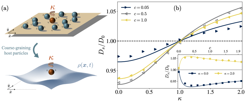
Figure 1: (a) Sketch of an odd-diffusing colloidal particle (red tracer with $\kappa\neq 0$) coupled via soft-core interactions to a medium of normally diffusing colloidal particles (blue host particles with $\kappa=0$). In the mesoscopic description discussed here, the host particles are accounted for in terms of the fluctuating density field $\rho(\bi{x},t)$. (b) Analytical (perturbative) predictions (solid lines) are compared with the results of Brownian dynamics simulation (symbols) for the long-time self-diffusion coefficient $D_{\mathrm{s}}/D_{0}$ of the odd tracer coupled to normal host particles as a function of the oddness parameter $\kappa$, see Eq. (35). For sufficiently small values of $\kappa$, the self-diffusion $D_{\mathrm{s}}$ is reduced compared to the the value $D_{0}$ it takes for an odd tracer in the absence of interactions with the host particles, as intuitively expected in a crowded environment. For $\kappa>\kappa_{c}=1$, however, the interaction of the tracer with the host particles enhances its self-diffusion. This phenomenon persists for a remarkably wide range of the density $c$. Note that at higher densities ($c=1.0$) the relative reduction/enhancement of the self diffusion is smaller than at intermediate densities ($c=0.5$). This can be understood by the self-diffusion anomaly of the GCM (non-monotonic dependence of the self-diffusion coefficient $D_{\mathrm{s}}$ as a function of the density, highlighted in the inset of panel (b). The simulation parameters to obtain panel (b) are: $N=200$ particles of mass $m=0.01$, friction coefficient $\gamma=1.0$, thermal energy $T=1.0$, particle diametre $\sigma=1.0$, and $\bar{\lambda}=1.0$ (see definition in Eq. (34)). For further details on the simulations see D.

2 The model

We consider the stochastic dynamics in $d=2$ spatial dimensions of an ensemble of $N+1$ interacting particles with positions $\bi{X}_{j}(t)\in\mathbb{R}^{2}$ at time $t$, and $j\in\{0,\ldots,N\}$. A sketch of the system is shown in Fig. 1(a). The particle labelled by $\bi{X}_{0}$ is characterised by an odd-diffusive behaviour and its dynamics follow an underdamped equation of motion. We refer to this particle as the odd tracer. In particular, the effect of oddness is encoded in the fact that its friction tensor $\bi{\Gamma}=\gamma[\mathbf{1}-\kappa\boldsymbol{\epsilon}]$ is characterised by antisymmetric elements proportional to the dimensionless oddness parameter $\kappa$, which stem from a non-conservative force experienced by the tracer [28, 79]. Here, $\gamma$ denotes the scalar friction coefficient. In the overdamped limit, this effect results in the odd diffusion tensor $\bi{D}=T\bi{\Gamma}^{-1}=D_{0}(\mathbf{1}+\kappa\boldsymbol{\epsilon})$, where $D_{0}=T/(\gamma(1+\kappa^{2}))$ is the scalar diffusion coefficient of a free odd particle [28], and $T$ is the temperature of the thermal bath measured in units such that the Boltzmann constant is one. We denote with $\boldsymbol{\epsilon}$ the two-dimensional antisymmetric Levi-Civita symbol ($\epsilon_{xx}=\epsilon_{yy}=0$ and $\epsilon_{xy}=-\epsilon_{yx}=1$) and with $\mathbf{1}$ the identity matrix. The stochastic dynamics of the odd tracer can be written as

$$\dot{\bi{X}}_{0} =\bi{V}_{0},$$ (1)

$$m\dot{\bi{V}}_{0} =-\lambda_{\mathrm{tr}}\sum_{j=1}^{N}\nabla\mathcal{U}(\bi{X}_{0}-\bi{X}_{j})-\bi{\Gamma}\bi{V}_{0}+\sqrt{2T\gamma}\,\boldsymbol{\xi}_{0},$$ (2)

where $\bi{V}_{0}(t)$ denotes the velocity of the odd tracer at time $t$, $m$ its mass, $\lambda_{\mathrm{tr}}$ is the overall strength of its interaction $\mathcal{U}$ with the host particles, while $\boldsymbol{\xi}_{0}$ belongs to a set of $N+1$ independent zero-mean Gaussian white noises $\{\boldsymbol{\xi}_{i}\}_{i=0}^{N}$ with correlation

$$\langle\boldsymbol{\xi}_{i}(t)\otimes\boldsymbol{\xi}_{j}(s)\rangle=\delta_{ij}\,\delta(t-s)\,\mathbf{1}.$$ (3)

Here, the symbol $\otimes$ denotes the outer product between two vectors $\bi{a}$ and $\bi{b}$, so that $[\bi{a}\otimes\bi{b}]_{\alpha\beta}=a_{\alpha}b_{\beta}$. The interaction potential $\mathcal{U}$ in Eq. (2) is assumed to be pairwise and with a smooth behaviour at the origin, such that $\nabla\mathcal{U}(\mathbf{0})=0$. Although we are ultimately interested in investigating the self-diffusion of the odd tracer in the overdamped regime, in which inertial effects can be neglected compared to viscous forces, we keep the time scale $\tau_{\gamma}=m/\gamma$ finite throughout the derivation, and take the limit $m\to 0$ at the end of the calculation because the stochastic description of an overdamped odd particle bears some non-trivial subtleties [28, 29]. As shown in A, the velocity $\bi{V}_{0}$ can be marginalised out at the level of the stochastic dynamics, leading to the following equation of motion for the position of the odd tracer

$$\dot{\bi{X}}_{0}= -\frac{\lambda_{\mathrm{tr}}}{m}\int_{t_{0}}^{t}\mathrm{d}s\,\bi{G}(t-s)\sum_{j=1}^{N}\nabla\mathcal{U}(\bi{X}_{0}(s)-\bi{X}_{j}(s))$$ (4)

$$+\bi{G}(t-t_{0})\bi{V}_{0}(t_{0})+\boldsymbol{\eta}(t),$$

where the memory matrix $\bi{G}(u)$ is defined as

$$\bi{G}(u) =\mathrm{e}^{-|u|/\tau_{\gamma}}\bi{M}(u),$$ (5)

$$\bi{M}(u) =\left(\begin{array}[]{cc}\cos(u\kappa/\tau_{\gamma})&\sin(u\kappa/\tau_{\gamma})\\ -\sin(u\kappa/\tau_{\gamma})&\cos(u\kappa/\tau_{\gamma})\end{array}\right)\,,$$ (8)

and $t_{0}$ is the time at which the initial conditions are imposed. Odd diffusion thus introduces oscillations in the dynamics of the tracer which decay on a time-scale $\tau_{\gamma}$ and vanish in the limit of a normal-diffusive system, i.e., $\bi{G}(u)\to\mathrm{exp}(-|u|/\tau_{\gamma})\,\mathbf{1}$ as $\kappa\to 0$. The memory introduced by the coarse-graining of the velocity appears in the convolution of $\bi{G}(u)$ with the interaction forces, as well as in the zero-mean Gaussian coloured noise

$$\boldsymbol{\eta}(t)=\frac{\sqrt{2T\gamma}}{m}\int_{t_{0}}^{t}\mathrm{d}s\,\bi{G}(t-s)\boldsymbol{\xi}_{0}(s),$$ (9)

with correlation

$$\langle\boldsymbol{\eta}(t)\otimes\boldsymbol{\eta}(s)\rangle=\frac{T}{m}\left[\mathrm{e}^{-|t-s|/\tau_{\gamma}}-\mathrm{e}^{-(t+s-2t_{0})/\tau_{\gamma}}\right]\bi{M}(t-s).$$ (10)

At long times $t-t_{0},s-t_{0}\gg\tau_{\gamma}$, the effect of the initial conditions is forgotten and the two-point correlation function above becomes time-translation invariant and reads

$$\langle\boldsymbol{\eta}(t)\otimes\boldsymbol{\eta}(s)\rangle\simeq\frac{T}{m}\bi{G}(t-s),\quad t,s\gg t_{0},$$ (11)

which corresponds to the noise correlation reported in Ref. [28]. In the same spirit as Refs. [76, 75], we find it convenient to describe the particles constituting the host medium in terms of their density field. Indeed, we are not interested in the microscopic details of the crowding host particles, but only in investigating the extent to which they affect the dynamics of the odd tracer. To this aim, following Ref. [72], we introduce the fluctuating particle density

$$\rho(\bi{x},t)=\sum_{j=1}^{N}\delta(\bi{x}-\bi{X}_{j}(t))\,,$$ (12)

and use it in order to formulate a mesoscopic description of the medium based on the microscopic one. The dynamics of the tracer can be specified from Eq. (4) as

$$\dot{\bi{X}}_{0} =-\frac{\lambda_{\mathrm{tr}}}{m}\int_{t_{0}}^{t}\mathrm{d}s\,\bi{G}(t-s)\int\mathrm{d}\bi{x}\,\nabla\mathcal{U}(\bi{X}_{0}(s)-\bi{x})\,\rho(\bi{x},s)$$ (13)

$$\quad+\bi{G}(t-t_{0})\bi{V}_{0}(t_{0})+\boldsymbol{\eta}(t)\,.$$

The stochastic evolution of the density $\rho(\bi{x},t)$ appearing in the previous equation can be determined on the basis of the microscopic dynamics of the $N$ host particles. In the overdamped regime the dynamics are

$$\dot{\bi{X}}_{j} =-\frac{\lambda_{\mathrm{ho}}}{\gamma}\sum_{k=1}^{N}\nabla\mathcal{U}(\bi{X}_{j}-\bi{X}_{k})-\frac{\lambda_{\mathrm{tr}}}{\gamma}\nabla\mathcal{U}(\bi{X}_{j}-\bi{X}_{0})+\sqrt{2T/\gamma}\,\boldsymbol{\xi}_{j},$$ (14)

where $j\in\{1,...,N\}$. Here we assume that the potential which acts between the various pairs of host particles is, up to an overall constant $\lambda_{\mathrm{ho}}/\lambda_{\mathrm{tr}}$, the same as that which determines the interaction $\lambda_{\mathrm{tr}}\mathcal{U}$ between each host particle and the tracer. Analogously to the original works by Kawasaki [73] and Dean [72], the stochastic dynamics of $\rho(\bi{x},t)$ can be derived using Itô’s lemma, and it turns out to be governed by the following continuity equation

$$\frac{\partial}{\partial t}\rho(\bi{x},t)=-\nabla_{\bi{x}}\cdot\bi{\mathcal{J}}(\bi{x},t)\,,$$ (15)

with the fluctuating flux

$$\bi{\mathcal{J}}(\bi{x},t) =-\frac{\lambda_{\mathrm{ho}}}{\gamma}\int\mathrm{d}\bi{y}\,\rho(\bi{y},t)\,\nabla\mathcal{U}(\bi{x}-\bi{y})\,\rho(\bi{x},t)-\frac{\lambda_{\mathrm{tr}}}{\gamma}\,\nabla\mathcal{U}(\bi{x}-\bi{X}_{0})\,\rho(\bi{x},t)$$ (16)

$$\quad-\frac{T}{\gamma}\,\nabla\rho(\bi{x},t)+\sqrt{2T\,\rho(\bi{x},t)/\gamma}\,\boldsymbol{\Lambda}(\bi{x},t).$$

A few comments on the above equation are in order: the first line on the r.h.s. corresponds to the drift flux due to the soft interactions between the host particles in the medium, and to the interaction between the density field of the host particles and the odd tracer at position $\bi{X}_{0}$. The second line, instead, stems from the coupling of the density $\rho(\bi{x},t)$ with the equilibrium thermal bath at temperature $T$. This involves the standard diffusive flux proportional to $\nabla\rho$ and a fluctuating contribution that depends on the zero-mean Gaussian white noise field $\boldsymbol{\Lambda}(\bi{x},t)$. The latter is characterised by the correlation

$$\langle\boldsymbol{\Lambda}(\bi{x},t)\otimes\boldsymbol{\Lambda}(\bi{y},s)\rangle=\delta(t-s)\,\delta(\bi{x}-\bi{y})\,\mathbf{1}.$$ (17)

Note that the noise $\sqrt{2T\,\rho(\bi{x},t)/\gamma}\,\boldsymbol{\Lambda}(\bi{x},t)$ is multiplicative as its amplitude depends on the fluctuating density itself and is to be interpreted in the Itô sense. Moreover, Eq. (15) is nonlinear in the density $\rho$, thus it cannot be solved analytically. In order to overcome this problem, we assume that the density fluctuations are much smaller than the homogeneous bulk density (see, e.g., Refs. [80, 81, 76, 75, 82]). In other words, we decompose the fluctuating density as $\rho(\bi{x},t)=\rho_{0}+\phi(\bi{x},t)$, where $\rho_{0}=N/L^{2}$ is the density in the homogeneous state, $N$ the number of particles and $L$ the typical box size, while $\phi(\bi{x},t)$ represents the fluctuations around that state. Then we assume that $|\phi(\bi{x},t)|\ll\rho_{0}$, which is increasingly accurate in the regime of high densities [80]. At the lowest order in $\phi(\bi{x},t)/\rho_{0}$ from Eqs. (15) and (16), one gets the following linear dynamics for the field $\phi(\bi{x},t)$,

$$\frac{\partial}{\partial t}\phi(\bi{x},t) =\frac{\rho_{0}}{\gamma}\int\mathrm{d}\bi{y}\,\left[\lambda_{\mathrm{tr}}\,\delta(\bi{y}-\bi{X}_{0})+\lambda_{\mathrm{ho}}\,\phi(\bi{y},t)\right]\nabla_{\bi{x}}^{2}\mathcal{U}(\bi{x}-\bi{y})$$ (18)

$$\quad+\frac{T}{\gamma}\nabla^{2}\phi(\bi{x},t)+\zeta(\bi{x},t),$$

where we introduce the scalar zero-mean Gaussian white noise field $\zeta(\bi{x},t)$ with correlations

$$\langle\zeta(\bi{x},t)\zeta(\bi{y},s)\rangle=-\frac{2T\rho_{0}}{\gamma}\delta(t-s)\,\nabla_{\bi{x}}^{2}\delta(\bi{x}-\bi{y}).$$ (19)

Note that, in this context, $\rho_{0}/\gamma$ is often referred to as the field mobility coefficient [83]. In the regime of small density fluctuations, the microscopic equation of motion of the odd tracer derived from Eq. (13) becomes

$$\dot{\bi{X}}_{0} =-\frac{\lambda_{\mathrm{tr}}}{m}\int_{t_{0}}^{t}\mathrm{d}s\,\bi{G}(t-s)\int\mathrm{d}\bi{x}\,\nabla\mathcal{U}(\bi{X}_{0}(s)-\bi{x})\,\phi(\bi{x},s)$$ (20)

$$\quad+\bi{G}(t-t_{0})\bi{V}_{0}(t_{0})+\boldsymbol{\eta}(t)\,.$$

3 Self-diffusion of the odd tracer

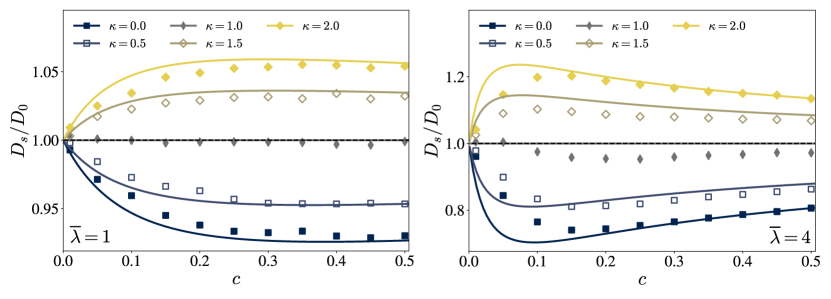
Figure 2: Analytical (perturbative) predictions (solid lines), see Eq. (35), and results of Brownian dynamics simulation results (symbols) for the long-time self-diffusion coefficient $D_{\mathrm{s}}/D_{0}$ of an odd tracer coupled to normally diffusive host particles as a function of the area fraction $c$ in two spatial dimensions, with interparticle potential $\mathcal{U}$ given by Eq. (33). (a) For an interaction coupling $\overline{\lambda}=1$ the self-diffusion $D_{\mathrm{s}}$ decreases upon increasing density $c$ of the medium for $\kappa<\kappa_{c}=1$, while it increases for $\kappa>\kappa_{c}$. Interestingly, at the critical value $\kappa_{c}$, the odd tracer diffuses at long times as in the absence of host particles, i.e., $D_{\mathrm{s}}=D_{0}$. (b) For a larger value of the coupling $\overline{\lambda}=4$, we observe that the enhancement of the self-diffusion for $\kappa>\kappa_{c}$ is much more pronounced (up to $20\%$), and the largest enhancement is obtained at a lower host medium density ($c\simeq 0.15$). The self-diffusion anomaly of the GCM model (i.e., the non-monotonic dependence of $D_{\mathrm{s}}$ on the host density) becomes evident for $\kappa<\kappa_{c}$ and is inverted for $\kappa>\kappa_{c}$. For the density getting higher, the GCM is known to exhibit a “high-density ideal gas”-like behaviour [57], a trend which we observe here as well. The simulation parameters used to obtain the two panels are the same as in figure 1. For further details on the simulations see D.

Using the evolution equations derived in the previous Section, we analyse the self-diffusion coefficient of the odd tracer and investigate how this is affected by the soft-core interactions with the host particles. Using a perturbative approach in the coupling strength $\lambda_{\mathrm{tr}}$ between the field $\phi(\bi{x},t)$ and the odd tracer, we compute the MSD of the latter and extract from its long-time behaviour the self-diffusivity defined as

$$D_{\mathrm{s}}=\lim_{(t-t_{0})\to\infty}\frac{\langle|\bi{X}_{0}(t)-\bi{X}_{0}(t_{0})|^{2}\rangle}{4(t-t_{0})}\,.$$ (21)

To this purpose, it is convenient to rewrite the stochastic dynamics of the field $\phi(\bi{x},t)$ in terms of its Fourier modes $\phi_{\bi{q}}(t)$, where the Fourier transform $f_{\bi{q}}$ of a function $f(\bi{x})$ is defined as $f_{\bi{q}}=\int\mathrm{d}\bi{x}\ f(\bi{x})\,\mathrm{exp}(-i\bi{x}\cdot\bi{q})$. The field dynamics of Eq. (18) becomes

$$\frac{\partial}{\partial t}\phi_{\bi{q}}=-\alpha_{\bi{q}}\phi_{\bi{q}}-\lambda_{\mathrm{tr}}\,\frac{\rho_{0}}{\gamma}q^{2}\mathcal{U}_{\bi{q}}\,\mathrm{e}^{-i\bi{q}\cdot\bi{X}_{0}}+\zeta_{\bi{q}}(t)\,,$$ (22)

where we introduced the inverse relaxation time

$$\alpha_{\bi{q}}=(\lambda_{\mathrm{ho}}\rho_{0}\,\mathcal{U}_{\bi{q}}+T)\,q^{2}/\gamma$$ (23)

of the $\bi{q}$-mode of the field and the Fourier transform of the noise $\zeta_{\bi{q}}(t)$ with correlation

$$\langle\zeta_{\bi{q}}(t)\zeta_{\bi{p}}(s)\rangle=\frac{2T\rho_{0}\,q^{2}}{\gamma}\delta(t-s)\,(2\pi)^{2}\delta(\bi{q}+\bi{p})\,.$$ (24)

Importantly, the relaxation time $1/\alpha_{\mathbf{q}}$ of $\phi_{\bi{q}}$ increases upon decreasing $q^{2}\to 0$, eventually diverging for the $\bi{q}=\mathbf{0}$ mode. This is in agreement with the fact that the field $\phi(\bi{x},t)$ is a locally conserved quantity, which evolves according to the continuity equation given by Eq. (18). Note that the field evolution in Eq. (22) is formally analogous to the one reported in Refs. [84, 85, 86, 87] for the case of model B dynamics. The coupling between the odd tracer and the field in Eq. (20) can also be rewritten in terms of the modes $\phi_{\bi{q}}(t)$ and becomes

$$\dot{\bi{X}}_{0}(t) =-\frac{\lambda_{\mathrm{tr}}}{m}\int_{t_{0}}^{t}\mathrm{d}s\,\bi{G}(t-s)\int\frac{\mathrm{d}\bi{q}}{(2\pi)^{2}}\,i\bi{q}\mathcal{U}_{\bi{q}}\,\phi_{\bi{q}}(s)\,\mathrm{e}^{i\bi{q}\cdot\bi{X}_{0}(s)}$$ (25)

$$\quad+\bi{G}(t-t_{0})\bi{V}_{0}(t_{0})+\boldsymbol{\eta}(t)\,.$$

In the next Section, we use Eqs. (25) and (22) as the starting point for the weak-coupling approximation.

3.1 Weak–coupling approximation

To compute the MSD, we formally expand the tracer position and the density field in powers of the coupling strength $\lambda_{\mathrm{tr}}$. This technique was put forward by Refs. [88, 85, 84] and adopted from a perturbative expansion of the generating functional of the dynamics within a path-integral formalism [89, 80, 90, 91]. The formal expansion of the tracer position and field reads

$$\bi{X}_{0}(t) =\sum_{n=0}^{\infty}\lambda_{\mathrm{tr}}^{n}\bi{X}_{0}^{(n)}(t)\,,$$ (26)

$$\phi_{\bi{q}}(t) =\sum_{n=0}^{\infty}\lambda_{\mathrm{tr}}^{n}\phi_{\bi{q}}^{(n)}(t).$$ (27)

Following Refs. [88, 85, 84] we use Eqs. (26) and (27) to obtain a series expansion for the MSD of the tracer,

$$\langle|\bi{X}_{0}(t)|^{2}\rangle =\left\langle\bi{X}_{0}^{(0)}(t)\cdot\bi{X}_{0}^{(0)}(t)\right\rangle$$ (28)

$$\quad+\lambda_{\mathrm{tr}}^{2}\left(\left\langle\bi{X}_{0}^{(1)}(t)\cdot\bi{X}_{0}^{(1)}(t)\right\rangle+2\left\langle\bi{X}_{0}^{(0)}(t)\cdot\bi{X}_{0}^{(2)}(t)\right\rangle\right)$$

$$\quad+\mathcal{O}(\lambda_{\mathrm{tr}}^{4}),$$

up to corrections of order $\mathcal{O}(\lambda_{\mathrm{tr}}^{4})$ and where we assumed that the initial position of the tracer is $\bi{X}_{0}(t_{0})=\mathbf{0}$ without loss of generality. However, the accuracy of the results obtained with the truncated series has to be checked a posteriori with numerical simulations. Importantly, all contributions related to odd powers of $\lambda_{\mathrm{tr}}$ vanish as the equations of motion are invariant under the transformation $(\lambda_{\mathrm{tr}},\phi)\leftrightarrow(-\lambda_{\mathrm{tr}},-\phi)$ [88, 84]. In order to evaluate the MSD we thus have to solve the set of coupled stochastic dynamics for the tracer and the field, Eqs. (25) and (22), respectively, at different orders of the expansion in $\lambda_{\mathrm{tr}}$. At the lowest order $\mathcal{O}(\lambda_{\mathrm{tr}}^{0})$ we find

$$\dot{\bi{X}}^{(0)}_{0}(t)=\bi{G}(t-t_{0})\bi{V}_{0}(t_{0})+\boldsymbol{\eta}(t)\,,$$ (29)

which determines the time evolution of the tracer particle in the absence of the interaction of the medium and is solved in B. The tracer evolution to linear order $\mathcal{O}(\lambda_{\mathrm{tr}}^{1})$ becomes

$$\dot{\bi{X}}_{0}^{(1)}(t) =-\frac{1}{m}\int_{t_{0}}^{t}\mathrm{d}s\ \bi{G}(t-s)\int\frac{\mathrm{d}\bi{q}}{(2\pi)^{2}}\,i\bi{q}\,\mathcal{U}_{\bi{q}}\,\phi_{\bi{q}}^{(0)}(s)\,\mathrm{e}^{i\bi{q}\cdot\bi{X}_{0}^{(0)}(s)},$$ (30)

which depends on the free field $\phi_{\bi{q}}^{(0)}$ and the free tracer $\bi{X}_{0}^{(0)}$. Similarly, at order $\mathcal{O}(\lambda_{\mathrm{tr}}^{2})$ we find

$$\dot{\bi{X}}_{0}^{(2)}(t)=-\frac{1}{m}\int_{t_{0}}^{t}\mathrm{d}s\ \bi{G}(t-s)\int\frac{\mathrm{d}\bi{q}}{(2\pi)^{2}}\,i\bi{q}\,\mathcal{U}_{\bi{q}}$$

$$\times\left[\phi_{\bi{q}}^{(1)}(s)+i\bi{q}\cdot\bi{X}_{0}^{(1)}(s)\,\phi_{\bi{q}}^{(0)}(s)\right]\mathrm{e}^{i\bi{q}\cdot\bi{X}_{0}^{(0)}(s)},$$

which, again, is related to the tracer position and the field at lower orders in the interaction coupling. The relevant correlations within the weak-coupling approximations, i.e., $\langle\bi{X}_{0}^{(1)}(t)\cdot\bi{X}_{0}^{(1)}(t)\rangle$ and $\langle\bi{X}_{0}^{(0)}(t)\cdot\bi{X}_{0}^{(2)}(t)\rangle$, are evaluated in C, Eqs. (C) and (C) respectively. In particular, in the overdamped regime $m\to 0$, the expressions for $\langle\bi{X}_{0}^{(1)}(t)\cdot\bi{X}_{0}^{(1)}(t)\rangle$ and $\langle\bi{X}_{0}^{(0)}(t)\cdot\bi{X}_{0}^{(2)}(t)\rangle$ simplify significantly, Eqs. (65) and (C) respectively. There our theoretical approach yields

$$\frac{D_{\mathrm{s}}}{D_{0}}=1-\frac{\lambda_{\mathrm{tr}}^{2}\rho_{0}}{2\gamma^{2}}\frac{1-\kappa^{2}}{1+\kappa^{2}}\int\frac{\mathrm{d}\bi{q}}{(2\pi)^{2}}\frac{q^{4}|\mathcal{U}_{\bi{q}}|^{2}}{\alpha_{\bi{q}}(\alpha_{\bi{q}}+D_{0}q^{2})}+\mathcal{O}(\lambda_{\mathrm{tr}}^{4})\,$$ (32)

for the self-diffusion coefficient, which constitutes the central result of the present work.

This equation predicts that the sign of the first non-trivial perturbative correction to the self-diffusion $D_{\mathrm{s}}$ is solely governed by the oddness parameter $\kappa$, due to the proportionality to the factor $(1-\kappa^{2})$. This implies that the critical value $\kappa_{c}=1$ separates two distinct regimes in which the interaction with the host medium suppresses ($\kappa<\kappa_{c}$) or enhances ($\kappa>\kappa_{c}$) the self-diffusion of the odd tracer; in particular, for $\kappa=\kappa_{c}$ we observe $D_{\mathrm{s}}=D_{0}$. Note that the specific value $\kappa_{c}=1$ of the critical oddness parameter, as well as the counter-intuitive independence of $\kappa_{c}$ on the density of the host medium, is expected to be accurate within the weak-coupling regime only. Furthermore, it is apparent from Eq. (32) that for some choices of the parameters the corrected self-diffusion $D_{s}$ becomes negative. This unphysical behaviour suggests that in those regions of the parameter space the weak-coupling approximation breaks down. Another important aspect to highlight is the fact that the derivation of Eq. (32) does not rely on the specific shape of the interaction potential $\mathcal{U}$.

3.2 Gaussian-core model

We proceed and specialise the predictions in Eq. (32) for the case of the Gaussian core model (GCM). Note that even though the host-host and host-tracer interactions can be different in principle, we restrict our analysis to identical interactions and coupling strengths $\lambda_{\mathrm{ho}}=\lambda_{\mathrm{tr}}=\lambda$. In the GCM, particles interact via the (bounded) Gaussian interaction potential

$$\mathcal{U}(\bi{x})=\frac{1}{2\pi\sigma^{2}}\exp\left(-\frac{\bi{x}^{2}}{2\sigma^{2}}\right).$$ (33)

The typical length scale of interaction is set by $\sigma$, which corresponds to the inter-particle distance at which the interaction force $\bi{F}(\bi{x})=-\lambda\nabla\mathcal{U}(\bi{x})$ is the strongest. Accordingly, we interpret $\sigma$ as an effective particle radius, which, in turn, defines a particle area of $\pi\sigma^{2}$ and thus an effective area fraction $c=\pi\sigma^{2}\rho_{0}=\pi\sigma^{2}N/L^{2}$. In the framework of the mesoscopic field theoretic description introduced in Sec. 2, the length scale $\sigma$ also determines the range of interaction between the odd tracer and the fluctuating density field $\phi(\bi{x},t)$. We note that, as apparent from Eq. (33), $\mathcal{U}$ has units $[\mathcal{U}]=1/\mathrm{m}^{2}$ and therefore $\lambda$ is dimensional with units $[\lambda]=\mathrm{Jm^{2}}$. For it to become an expansion parameter it thus needs to be made dimensionless by a typical energy and length scale of the system. To this aim, we use the length scale $\sigma$ and the thermal energy, obtaining

$$\lambda\to\overline{\lambda}=\frac{\lambda}{2\pi\sigma^{2}\,T},$$ (34)

such that $[\overline{\lambda}]=1$, defining $T$ to be measured in units such that the Boltzmann constant is unity. In related works, the phase diagram of the GCM is analysed and $1/\overline{\lambda}$ is used as an effective temperature [50, 58, 57]. The GCM, thereby, was found to exhibit an upper-freezing temperature at $1/\overline{\lambda}_{\mathrm{freez}}=0.0102$  [57], above which it behaves as a fluid for all densities. Our parameter choice in Figs. 1 and 2 ensures that the medium is in the fluid phase with $\overline{\lambda}\ll\overline{\lambda}_{\mathrm{freez}}$, see also D. The self-diffusion correction reported in Eq. (32) can now be expressed in terms of dimensionless quantities as

$$\frac{D_{\mathrm{s}}}{D_{0}}=1-2\pi\,\overline{\lambda}^{2}c\,\frac{1-\kappa^{2}}{1+\kappa^{2}}\int\frac{\mathrm{d}\bi{p}}{(2\pi)^{2}}\frac{|\mathcal{U}_{\bi{p}/\sigma}|^{2}}{\beta_{\bi{p}/\sigma}(\beta_{\bi{p}/\sigma}+\frac{1}{1+\kappa^{2}})}+\mathcal{O}(\overline{\lambda}^{4})\,,$$ (35)

where we introduced the rescaled wave vector $\bi{p}=\sigma\bi{q}$ and the dimensionless quantity $\beta_{\bi{q}}=(2\overline{\lambda}c\,\mathcal{U}_{\bi{q}}+1)$. Note that $\beta_{\bi{q}}$ is invariant under the transformation $(\overline{\lambda}\to a\overline{\lambda},c\to c/a)$ where $a>0$ is a constant coefficient, i.e., it assumes the same value if we consider a more diluted medium with stronger interaction coupling. Consequently, it is easy to verify that the first non-trivial correction to the self-diffusion depends linearly on $a$. Remember further that $D_{0}=T/(\gamma(1+\kappa^{2}))$ which leaves the factor of $1/(1+\kappa^{2})$ in the integrand of Eq. (35).

By specialising Eq. (35) to the GCM case and resorting to standard numerical integration schemes (see  C) for the evaluation of the momentum integral, we analyse the extent to which the long-time self-diffusion $D_{\mathrm{s}}$ of the odd tracer is affected by the interactions with the host medium. In Fig. 1(b) we show the behaviour of $D_{\mathrm{s}}$ as a function of the oddness parameter $\kappa$ and compare the theoretical predictions with Brownian dynamics simulations (see D for details). In particular, we observe that in the weak-coupling limit, when the oddness parameter $\kappa$ is smaller than its critical value $\kappa_{c}=1$, for all densities $c$ the self-diffusion of the odd tracer is suppressed compared to the value $D_{0}$, which characterises a single odd particle in the absence of interactions. This behaviour is expected and can be observed in various systems with repulsive interactions, e.g., in systems with hard-core [8, 9, 10, 11] or soft-core [16, 17] repulsion, but also for attractive Lennard-Jones particles [12, 13, 14, 15]. The decrease of the self-diffusion upon increasing the density of the particles in the medium reflects the intuition that in a crowded environment the motion of a diffusive tracer is hindered by the collisions with the other particles.

However, the combined effect of the particle interactions with the odd-diffusive motion of the tracer eventually results in an inversion of this tendency. For $\kappa>\kappa_{c}$, we observe an enhancement of the self-diffusion $D_{\mathrm{s}}$ compared to $D_{0}$, irrespective of the area fraction $c$. This phenomenology was first observed for the self-diffusion of odd-diffusive hard disks in Ref. [22] and since then was confirmed via theory and simulations for systems of particles with excluded volume [25, 24, 40]. Our finding proves that an enhancement of the self-diffusion is possible not only for systems of particles with hard-core repulsion, but also with generic bounded soft-core potentials, as shown in Eq. (32). At the same time, the fact of having soft-core interactions shifts the value of the critical oddness parameter to $\kappa_{c}=1$, while it was $\kappa_{c}=1/\sqrt{3}\approx 0.58$ in the case of hard disks [22]. This implies that in the case of soft-core interactions a more pronounced chirality is required to enhance the transport properties of the odd-tracer, as the effect of the collisions is “milder” in the presence of soft interactions.

One of the main advantages of the field-theoretic description adopted here compared to the geometric approach of Ref. [22], is that it allows us to extend the investigation to the case of dense systems. In particular, we show in Fig. 1(b) the dependence of $D_{\mathrm{s}}$ on $\kappa$ for very dilute ($c=5\%$, dark blue), moderately dense ($c=50\%$, grey), and very dense ($c=100\%$, yellow) systems of host particles. It appears that the behaviour of the self-diffusion as a function of the density is far from trivial. Focusing on values of $\kappa$ with $\kappa<\kappa_{c}$, $D_{\mathrm{s}}$ is larger when the tracer is dispersed in a very dense medium ($c=100\%$) than in the case of intermediate density ($c=50\%$). This seemingly counter-intuitive phenomenon of the GCM, referred to as the “self-diffusion anomaly”, is associated with the structural anomaly of the fluid GCM at high density [17, 64, 65, 66, 16, 92, 93]. Specifically, as the interaction potential is bounded, particles tend to overlap for sufficiently high densities, generating an entropic gain [17], and actually tend to display a “high-density ideal gas”-like behaviour for even higher densities [57], where $D_{\mathrm{s}}\uparrow D_{0}$. In the inset of Fig. 1(b), we show the emergence of this anomaly by investigating the dependence of $D_{\mathrm{s}}$ on $c$ over a wide range of densities up to $c=200\%$. For a normal diffusive tracer ($\kappa=0$), we confirm the non-monotonic anomalous behaviour of $D_{\mathrm{s}}$, which first sharply decreases and then slowly increases upon increasing $c$. However, $D_{\mathrm{s}}<D_{0}$ for all densities $c$. Surprisingly, however, for $\kappa>\kappa_{c}=1$, we observe a specular trend showing an initial increase of the self-diffusion $D_{\mathrm{s}}$ for sufficiently dilute systems, followed by a decrease as a function of $c$, when its value exceeds a certain threshold. Thus, for $\kappa>\kappa_{c}$, the self-diffusion anomaly of the GCM is inverted, $D_{\mathrm{s}}\downarrow D_{0}$, and remarkably $D_{\mathrm{s}}>D_{0}$ for all densities.

In Fig. 2 we plot the self-diffusion $D_{\mathrm{s}}$ as a function of the density $c$ up to $c=50\%$ for different values of the oddness parameter $\kappa$. In particular, panel (a) shows the predictions for a coupling parameter $\overline{\lambda}=1$ while panel (b) for $\overline{\lambda}=4$. Notably, the analytical predictions (solid lines) are in excellent agreement with the results of Brownian dynamics simulations (symbols), especially for denser systems. This is coherent with the fact that the linearisation of the Dean-Kawasaki equation in Eq. (15) provides more accurate results when the density fluctuations $\phi$ around the homogeneous bulk density $\rho_{0}$ are much smaller than $\rho_{0}$ itself. As anticipated by Fig. 1(b) and above, it turns out that $D_{\mathrm{s}}>D_{0}$ for $\kappa>\kappa_{\mathrm{c}}$, while $D_{\mathrm{s}}<D_{0}$ for $\kappa<\kappa_{\mathrm{c}}$. Particularly interesting in Fig. 2(a) is the critical case $\kappa=\kappa_{c}$, for which the self-diffusion appears to be insensitive to any variation of the medium density, and the tracer diffuses effectively as a free particle. This effect can be rationalised by noting that increasing the host density has a twofold effect on the tracer: on the one hand, it makes the surrounding environment more crowded, thus hindering the motion of the tracer; on the other hand, thanks to the mutual rolling mechanism analysed in Refs. [22, 24], the interaction with the host particles can speed up the dynamics of the odd tracer. At $\kappa=\kappa_{c}$ these two effects balance each other and the tracer effectively evolves as in the absence of interactions. Also in this case, Fig. 2(a) shows a remarkable agreement between analytical predictions and numerical data obtained from Brownian dynamics simulations. Importantly, the fact that $\kappa_{c}$ does not depend on the host medium density holds true only within the weak-coupling regime illustrated in panel (a) of Fig. 2, while it is not longer the case when the interaction strength $\overline{\lambda}$ is increased, as shown in panel (b) of Fig. 2.

With $\overline{\lambda}$ being chosen four times larger in Fig. 2(b) than in Fig. 2(a), the interaction-induced enhancement of $D_{\mathrm{s}}$ can reach $\approx 20\%$ of the free value $D_{0}$, compared to $\approx 5\%$ of Fig. 2(a), which agrees with the $\overline{\lambda}$ rescaling of the interaction-correction observed in Eq. (35). Upon increasing the value of the coupling $\overline{\lambda}$, the self-diffusion anomaly of the GCM is further observed starting from much lower densities ($c\approx 15\%$). In this case, the agreement between simulations and analytical predictions is slightly worse, specifically in the dilute regime due to the less accurate linearisation of Dean’s equation. Further, the matching is less accurate in the dense regime when the oddness parameter approaches $\kappa_{c}$. This observation can be rationalised by noting that when the interaction coupling $\overline{\lambda}$ is sufficiently large and $\kappa\approx\kappa_{c}$, the first non-trivial correction to $D_{\mathrm{s}}$ in Eq. (35) becomes comparable with higher-order terms $\mathcal{O}(\overline{\lambda}^{4})$, which are neglected in our analytical treatment.

4 Conclusions

In this work, we studied the self-diffusion coefficient $D_{\mathrm{s}}$ of an odd-diffusive tracer coupled to an ensemble of normally diffusive crowding host particles. The pairwise interaction between the particles was modelled by the bounded soft-core Gaussian potential, the so-called Gaussian core model (GCM), implying that distinct particles may partially overlap. From the microscopic picture of the GCM fluid, we moved to a field-theoretic description based on the Dean-Kawasaki equation [72, 73, 74] in which the host particles are coarse-grained into a thermally fluctuating density field $\rho(\bi{x},t)$. Under the assumption that the interaction coupling strength $\lambda$ between the density field and the odd tracer is sufficiently small, we obtained a perturbative expansion for the MSD of the latter, which we truncated at the first non-trivial order $\mathcal{O}(\lambda^{2})$. Based on this expansion we evaluated the field-induced correction to the self-diffusion of the odd tracer and compared it with Brownian dynamics simulations. In particular, we showed that, upon increasing the oddness parameter $\kappa$, the collisions with the host particles have a substantially different effect on the transport properties of the tracer. Specifically, there exists a critical value $\kappa_{c}$ of the oddness parameter $\kappa$ such that for $\kappa<\kappa_{c}$ the self-diffusion $D_{\mathrm{s}}$ is reduced by the crowding effect introduced by the host particles, i.e., $D_{\mathrm{s}}$ decreases upon increasing the overall host particle density $c$. In contrast, for $\kappa>\kappa_{c}$ the interaction with the host particles leads to an enhancement of the self-diffusion upon increasing $c$. Moreover, we showed that this enhancement reaches its maximum at a specific density of the system, whose value depends on the interaction coupling $\lambda$. Beyond that value, $D_{\mathrm{s}}$ starts decreasing upon increasing $c$. This non-monotonic behaviour of the self-diffusion as a function of the area fraction $c$ for $\kappa>\kappa_{c}$ is specular to that of normally diffusive Gaussian-core particles, for which the diffusion coefficient first sharply decreases and then slowly increases upon increasing the host density (see the self-diffusion anomaly of the GCM, discussed e.g., in Refs. [17, 64, 65, 66, 16]). Finally, we showed that at the critical value $\kappa=\kappa_{c}$ and within the weak-coupling regime, the self-diffusion of the odd tracer is not affected by the collisions with the crowding particles, irrespective of their density.

The model presented here can be extended to address a variety of related problems. For example, the Dean-Kawasaki equation has already been generalised to the underdamped regime, by including in the description a momentum density field [94, 95]. A potentially interesting direction is that of deriving the fluctuating hydrodynamic equations for a system of interacting odd-diffusive soft-core particles in the underdamped regime and then use it to study the dynamic behaviour of a tracer in such a medium. Moreover, the derivation presented here can be used for a systematic analysis of the role of mass on the transport properties of an odd tracer in a crowded environment, which we leave for future work.

The GCM is known to exhibit further anomalous properties beyond the self-diffusion anomaly discussed here, among which we mention a density anomaly (expansion upon isobaric cooling), a structural order anomaly (reduction of the short-range translational order upon isothermal compression) and a re-entrant melting transition for the solid GCM  [17, 66, 64, 67, 57]. As we showed here, the interplay between the odd diffusivity of the tracer and the self-diffusion anomaly (increase upon isothermal compression) of the underlying fluid gives rise to an interesting and unexpected behaviour of the self-diffusion coefficient (see Fig. 2(a)). It is therefore interesting to thoroughly investigate the influence of oddness on structural, transport and thermodynamic properties of the GCM.

For a binary mixture of GCM particles, previous work showed the existence of fluid-fluid phase separation [96, 97]. Coupling odd tracers to this kind of mixtures might show surprising behaviour in the dynamics of the transition. correlations on arbitrarily large length scales which could introduce fluctuation-induced forces between the odd-particles [98, 99, 100, 101, 85, 102]. Finally, in the formulation presented here, the odd tracer and the host particles (and thus the density field $\rho$) evolve according to an equilibrium dynamics. It may be interesting to analyse the transport properties of an (odd) tracer coupled to an active (odd) fluid featuring nonequilibrium fluctuations, in which the detailed balance condition is not fulfilled. The odd medium could be described by continuum models based on fluctuating density and polarity fields, as for example in Ref. [103], or with hydrodynamic theories characterised by odd viscosity [104], where already remarkable effects for tracers have been reported [105, 106, 43, 107, 108, 109, 110].

Appendix A Velocity marginalisation

In this Appendix we derive the equation of motion for the position of the odd tracer reported in Eq. (4) by integrating out the velocity variable $\bi{V}_{0}(t)$ from Eqs. (1) and (2). To this aim, we define the new variable $\bi{U}_{0}(t)=\bi{S}^{-1}\bi{V}_{0}(t)$, which is related to the velocity $\bi{V}_{0}(t)$ by a suitably chosen linear transformation $\bi{S}$. The latter has the property to diagonalise the friction tensor $\bi{\Gamma}$, and satisfies $\bi{S}^{-1}\,\bi{\Gamma}\bi{S}=\bi{L}$, with $\bi{L},\bi{S}\in\mathbb{C}^{2\times 2}$. In particular, $\bi{L}$ is diagonal and contains the eigenvalues of the friction tensor $L_{00}\equiv\ell_{0}=\gamma(1-i\kappa)$ and $L_{11}\equiv\ell_{1}=\gamma(1+i\kappa)$, where $i$ denotes the imaginary unit, while

$$\bi{S}=\frac{1}{\sqrt{2}}\left(\begin{array}[]{cc}-i&i\\ 1&1\end{array}\right).$$ (36)

Note that the emergence of complex eigenvalues is due to the oscillatory behaviour introduced by the oddness parameter $\kappa$. In the new variable $\bi{U}_{0}$, the dynamics of Eqs. (1) and (2) can be formally solved, yielding

$$\bi{U}_{0}(t) =\mathrm{e}^{-\frac{(t-t_{0})}{m}\bi{L}}\,\bi{U}_{0}(t_{0})-\frac{\lambda_{\mathrm{tr}}}{m}\int_{t_{0}}^{t}\mathrm{d}s\,\mathrm{e}^{-\frac{(t-s)}{m}\bi{L}}\sum_{j=0}^{N}\bi{S}^{-1}\,\nabla\mathcal{U}(\bi{X}_{0}(s)-\bi{X}_{j}(s))$$ (37)

$$\quad+\frac{1}{m}\int_{t_{0}}^{t}\mathrm{d}s\,\mathrm{e}^{-\frac{(t-s)}{m}\bi{L}}\,\bi{S}^{-1}\,\boldsymbol{\xi}_{0}(s).$$

The expression for $\bi{U}_{0}(t)$ can be inverted back into the original variables to find the stochastic dynamics of the position $\dot{\bi{X}}_{0}(t)=\bi{S}\bi{U}_{0}(t)$. Using the identity, obtained from straightforward computation,

$$S_{\alpha\beta}S^{-1}_{\beta\sigma}\,f_{\sigma}(s)\,\mathrm{exp}\left(-\frac{\ell_{\beta}}{m}(t-s)\right)=G_{\alpha\beta}(t-s)\,f_{\beta}(s)$$ (38)

where $\bi{f}(s)$ is a generic $2$-dimensional vector, $s<t$ and $\bi{G}(u)$ defined in Eq. (5) of the main text, Eq. (4) is finally obtained. Note that repeated indices imply summation according to the Einstein notation. As described in Eq. (9), the evolution of the position of the odd tracer depends on the colored noise $\boldsymbol{\eta}(t)$, which is given by the convolution of the function $\bi{G}(u)$ with the white noise $\boldsymbol{\xi}_{0}$. The correlation of $\boldsymbol{\eta}(t)$ can be computed as

$$\langle\boldsymbol{\eta}(t)\otimes\boldsymbol{\eta}(s)\rangle =\frac{2T\gamma}{m^{2}}\int_{t_{0}}^{t}\mathrm{d}t^{\prime}\int_{t_{0}}^{s}\mathrm{d}s^{\prime}\,\bi{G}(t-t^{\prime})\,\bi{G}^{\mathrm{T}}(s-s^{\prime})\,\delta(t^{\prime}-s^{\prime})$$ (39)

$$=\frac{2T\gamma}{m^{2}}\int_{t_{0}}^{\min{(t,s)}}\mathrm{d}t^{\prime}\,\bi{G}(t-t^{\prime})\,\bi{G}^{\mathrm{T}}(s-t^{\prime})$$

$$=\frac{T}{m}\left[\mathrm{e}^{-|t-s|/\tau_{\gamma}}-\mathrm{e}^{-(t+s-2t_{0})/\tau_{\gamma}}\right]\bi{M}(t-s),$$

which corresponds to the correlation reported in Eq. (10) of the main text, and $\bi{M}$ is given by Eq. (8). For the matrix product in the above calculation we used the relation

$$\bi{G}(t-t^{\prime})\,\bi{G}^{T}(s-t^{\prime})=\mathrm{e}^{-(t+s-2t^{\prime})/\tau_{\gamma}}\,\bi{M}(t-s),$$ (40)

which easily can be shown with the help of trigonometric identities.

Appendix B Tracer dynamics in the absence of interaction with the medium

We here analyse the case in which the coupling between the odd tracer and the density field of the particles in the medium is switched off. We denote the position of such a free odd tracer as $\bi{X}_{0}^{(0)}$, and the free field as $\phi_{\bi{q}}^{(0)}$.

B.1 Free dynamics of the odd tracer

In the absence of the coupling to the field, i.e., $\lambda_{\mathrm{tr}}=0$, the stochastic dynamics of the odd tracer in Eq. (29) can be exactly solved, and yields

$$\bi{X}^{(0)}_{0}(t)=\int_{t_{0}}^{t}\mathrm{d}s\,\bi{G}(s-t_{0})\,\bi{V}_{0}(t_{0})+\int_{t_{0}}^{t}\mathrm{d}s\,\boldsymbol{\eta}(s),$$ (41)

where we assumed that the odd tracer is initially at $\bi{X}^{(0)}_{0}(t_{0})=\mathbf{0}$, without loss of generality. Note that $\bi{V}_{0}(t_{0})$ is an assigned value and therefore does not need a perturbative expansion. As the position $\bi{X}^{(0)}_{0}$ of the tracer follows a Gaussian process, we can characterise it by its mean $\boldsymbol{\mu}_{0}(t)\equiv\langle\bi{X}^{(0)}_{0}(t)\rangle$ and two-time connected correlation function $\bi{C}(t,s)$. From Eq. (41) these quantities can be straightforwardly obtained, yielding

$$\boldsymbol{\mu}_{0}(t)=m\,\bi{A}(t-t_{0})\bi{V}_{0}(t_{0}),$$ (42)

and

$$\bi{C}(t,s) \equiv\left\langle\bi{X}_{0}^{(0)}(t)\otimes\bi{X}_{0}^{(0)}(s)\right\rangle-\left\langle\bi{X}_{0}^{(0)}(t)\right\rangle\,\otimes\left\langle\bi{X}_{0}^{(0)}(s)\right\rangle$$ (43)

$$=2D_{0}\,\left[\min(s,t)-t_{0}\right]\,\mathbf{1}-mT\left[\bi{\Gamma}^{-1}\bi{A}(t-t_{0})+(\bi{\Gamma}^{-1}\bi{A}(s-t_{0}))^{\mathrm{T}}\right]$$

$$\quad+mT\left[\Theta(t-s)\,\bi{\Gamma}^{-1}\bi{A}(t-s)+\Theta(s-t)\,(\bi{\Gamma}^{-1}\bi{A}(s-t))^{\mathrm{T}}\right]$$

$$\quad-mT\bi{A}(t-t_{0})\bi{A}^{\mathrm{T}}(s-t_{0}),$$

where we introduced the abbreviation $\bi{A}(u)=\bi{\Gamma}^{-1}[\mathbf{1}-\bi{G}(u)]$. We denoted by $\bi{a}\otimes\bi{b}=a_{\alpha}b_{\beta}$ the outer product between two vectors $\bi{a}$ and $\bi{b}$, and we introduced the bare diffusion coefficient $D_{0}=T/(\gamma(1+\kappa^{2}))$ of the odd tracer. Note that the connected correlation satisfies $\bi{C}(t,s)=\bi{C}^{\mathrm{T}}(s,t)$. Once $\boldsymbol{\mu}_{0}(t)$ and $\bi{C}(t,s)$ are known, we can compute the generating functional $\mathcal{Z}[\bi{j}]$ of the $n$-point correlations for the position of the odd tracer in the free case ($\lambda_{\mathrm{tr}}=0$),

$$\mathcal{Z}[\bi{j}]=\left\langle\exp\left\{\int\mathrm{d}t\,\bi{j}(t)\cdot\bi{X}^{(0)}_{0}(t)\right\}\right\rangle\,,$$ (44)

where $\bi{j}(t)$ is an auxiliary field and the average is taken with respect to the Gaussian path probability

$$\mathcal{P}_{0}[\bi{x}]\propto\exp \Bigg{\{}-\frac{1}{2}\int\mathrm{d}t\int\mathrm{d}s\,[\bi{x}(t)-\boldsymbol{\mu}_{0}(t)]\cdot\bi{C}(t,s)\,[\bi{x}(s)-\boldsymbol{\mu}_{0}(s)]\Bigg{\}}.$$ (45)

Solving the functional Gaussian integral in Eq. (44) leads to the expression

$$\mathcal{Z}[\bi{j}]=\exp \Bigg{\{}\frac{1}{2}\int\mathrm{d}t\int\mathrm{d}s\,\bi{j}(t)\cdot\bi{C}(t,s)\,\bi{j}(s)+\int\mathrm{d}t\,\bi{j}(t)\cdot\boldsymbol{\mu}_{0}(t)\Bigg{\}}$$ (46)

for the generating functional. The explicit expression of this generating functional will be particularly useful for deriving some of the expressions presented further below, see Eq. (53).

B.2 Free dynamics of the field

In the absence of interactions with the tracer particle, the dynamics of the free field in Fourier space $\phi^{(0)}_{\bi{q}}$ follows an Ornstein-Uhlenbeck process, solved by

$$\phi_{\bi{q}}^{(0)}(t)=\phi_{\bi{q}}^{(0)}(t_{0})\,\mathrm{e}^{-\alpha_{\bi{q}}(t-t_{0})}+\int_{t_{0}}^{t}\mathrm{d}s\,\mathrm{e}^{-\alpha_{\bi{q}}(t-s)}\,\zeta_{\bi{q}}(s).$$ (47)

Here, $\phi_{\bi{q}}(t)=\int\mathrm{d}\bi{x}\ \phi(\bi{x},t)\ \mathrm{exp}(-i\bi{x}\cdot\bi{q})$ denotes the (two-dimensional) Fourier transform of a field $\phi(\bi{x},t)$ with wave vector $\bi{q}$. From Eq. (47) we compute the two-point correlations of the free field as

$$\left\langle\phi_{\bi{q}}^{(0)}(t)\,\phi_{\bi{p}}^{(0)}(s)\right\rangle=\left\langle\phi_{\bi{q}}^{(0)}(t_{0})\,\phi_{\bi{p}}^{(0)}(t_{0})\right\rangle\,\mathrm{e}^{-\alpha_{\bi{q}}(t-t_{0})}\,\mathrm{e}^{-\alpha_{\bi{p}}(s-t_{0})}$$

$$\qquad\qquad+\frac{T}{\lambda_{\mathrm{ho}}\mathcal{U}_{\bi{q}}+T/\rho_{0}}\left[\mathrm{e}^{-\alpha_{\bi{q}}|t-s|}-\mathrm{e}^{-\alpha_{\bi{q}}(t+s-2t_{0})}\right]\,(2\pi)^{2}\delta(\bi{q}+\bi{p}),$$ (48)

where we used that $\mathcal{U}_{\bi{q}}=\mathcal{U}_{-\bi{q}}$ which holds for any symmetric interaction potential. When $t=s$ and the field had sufficient time to relax (formally $t_{0}\to-\infty$), the two-point correlator yields

$$\left\langle\phi_{\bi{q}}^{(0)}(t)\,\phi_{\bi{p}}^{(0)}(t)\right\rangle=\frac{T}{\lambda_{\mathrm{ho}}\mathcal{U}_{\bi{q}}+T/\rho_{0}}\,(2\pi)^{2}\delta(\bi{q}+\bi{p}).$$ (49)

Thus, if we assume that the field is distributed according to its equilibrium distribution before being put in contact with the odd tracer at time $t=t_{0}$, then $\langle\phi_{\bi{q}}^{(0)}(t_{0})\,\phi_{\bi{p}}^{(0)}(t_{0})\rangle$ is given by Eq. (49). Under this assumption, Eq. (B.2) can be written as

$$\left\langle\phi_{\bi{q}}^{(0)}(t)\,\phi_{\bi{q}^{\prime}}^{(0)}(s)\right\rangle =(2\pi)^{2}\delta(\bi{q}+\bi{p})\,\frac{T}{\lambda_{\mathrm{ho}}\mathcal{U}_{\bi{q}}+T/\rho_{0}}\mathrm{e}^{-\alpha_{\bi{q}}|t-s|}$$ (50)

$$\equiv(2\pi)^{2}\delta(\bi{q}+\bi{p})\,C_{\phi_{\bi{q}}}(t-s),$$

which defines the stationary time-translational invariant correlator $C_{\phi_{\bi{q}}}$ of the free field $\phi_{\bi{q}}^{(0)}$, which will be of importance later, see Eqs. (C) and (53).

Appendix C Weak-coupling approximation

In this Appendix, we compute the first non-trivial perturbative correction to the MSD which, due to the symmetry $(\lambda_{\mathrm{tr}},\phi)\leftrightarrow(-\lambda_{\mathrm{tr}},-\phi)$ is of second order in the interaction coupling $\lambda_{\mathrm{tr}}$. In the case in which the tracer is initialised at the origin, i.e., for $\bi{X}_{0}(t_{0})=\mathbf{0}$, this is formally given by Eq. (28). In order to evaluate this correction, we need to separately compute the correlations $\langle\bi{X}_{0}^{(1)}(t)\cdot\bi{X}_{0}^{(1)}(t)\rangle$ and $\langle\bi{X}_{0}^{(0)}(t)\cdot\bi{X}_{0}^{(2)}(t)\rangle$. To evaluate the first, we formally solve the stochastic dynamics in Eq. (30) to get

$$\left\langle\bi{X}_{0}^{(1)}(t)\cdot\bi{X}_{0}^{(1)}(t)\right\rangle=-\frac{1}{m^{2}}\int\frac{d\bi{q}}{(2\pi)^{2}}\int\frac{d\bi{p}}{(2\pi)^{2}}\,q_{\beta}p_{\gamma}\,\mathcal{U}_{\mathrm{t},\bi{q}}\,\mathcal{U}_{\mathrm{t},\bi{p}}$$

$$\qquad\times\int_{t_{0}}^{t}\mathrm{d}s\int_{t_{0}}^{s}\mathrm{d}u\int_{t_{0}}^{t}\mathrm{d}s^{\prime}\int_{t_{0}}^{t}\mathrm{d}u^{\prime}\,G_{\alpha\beta}(s-u)\,G_{\alpha\gamma}(s^{\prime}-u^{\prime})$$

$$\qquad\times\left\langle\phi_{\bi{q}}^{(0)}(u)\,\phi_{\bi{p}}^{(0)}(u^{\prime})\,\mathrm{e}^{i\bi{q}\cdot\bi{X}_{0}^{(0)}(u)+i\bi{p}\cdot\bi{X}_{0}^{(0)}(u^{\prime})}\right\rangle.$$ (51)

As the average in the last line only involves the position $\phi_{\bi{q}}^{(0)}$ of the free tracer $\bi{X}_{0}^{(0)}$ and the free field, it can be factorised as follows

$$\left\langle\phi_{\bi{q}}^{(0)}(u)\,\phi_{\bi{p}}^{(0)}(u^{\prime})\,\mathrm{e}^{i\bi{q}\cdot\bi{X}_{0}^{(0)}(u)+i\bi{p}\cdot\bi{X}_{0}^{(0)}(u^{\prime})}\right\rangle$$

$$\qquad=\left\langle\phi_{\bi{q}}^{(0)}(u)\,\phi_{\bi{p}}^{(0)}(u^{\prime})\right\rangle\left\langle\mathrm{e}^{i\bi{q}\cdot\bi{X}_{0}^{(0)}(u)+i\bi{p}\cdot\bi{X}_{0}^{(0)}(u^{\prime})}\right\rangle$$

$$\qquad=(2\pi)^{2}\delta(\bi{q}+\bi{p})\,C_{\phi_{\bi{q}}}(u-u^{\prime})\,\mathcal{Q}_{\bi{q}}(u,u^{\prime})$$ (52)

where we used Eq. (50) and we introduced the two-time quantity $\mathcal{Q}_{\bi{q}}$, which can be obtained from the generating functional as

$$\mathcal{Q}_{\bi{q}}(u,u^{\prime}) \equiv\mathcal{Z}[\bi{j}=i\bi{q}(\delta(t-u)-\delta(t-u^{\prime}))]$$ (53)

$$=\exp\Big{\{}-\frac{1}{2}\bi{q}\cdot[\bi{C}(u,u)+\bi{C}(u^{\prime},u^{\prime})]\bi{q}$$

$$\quad+\frac{1}{2}\bi{q}\cdot[\bi{C}(u^{\prime},u)+\bi{C}(u,u^{\prime})]\bi{q}+i\bi{q}\cdot[\boldsymbol{\mu}_{0}(u)-\boldsymbol{\mu}_{0}(u^{\prime})]\Big{\}}$$

Therefore, the correlation $\langle\bi{X}_{0}^{(1)}(t)\cdot\bi{X}_{0}^{(1)}(t)\rangle$ in Eq. (C) can be rewritten as

$$\left\langle\bi{X}_{0}^{(1)}(t)\cdot\bi{X}_{0}^{(1)}(t)\right\rangle=\frac{1}{m^{2}}\int\frac{d\bi{q}}{(2\pi)^{2}}\,q_{\beta}q_{\gamma}\,|\mathcal{U}_{\mathrm{t},\bi{q}}|^{2}$$

$$\qquad\times\int_{t_{0}}^{t}\mathrm{d}s\int_{t_{0}}^{s}\mathrm{d}u\int_{t_{0}}^{t}\mathrm{d}s^{\prime}\int_{t_{0}}^{s^{\prime}}\mathrm{d}u^{\prime}\,G_{\alpha\beta}(s-u)G_{\alpha\gamma}\,(s^{\prime}-u^{\prime})$$

$$\qquad\times C_{\phi_{\bi{q}}}(u-u^{\prime})\,\mathcal{Q}_{\bi{q}}(u,u^{\prime}).$$ (54)

Before calculating $\langle\bi{X}_{0}^{(0)}(t)\cdot\bi{X}_{0}^{(2)}(t)\rangle$ it is convenient to solve the dynamics of $\phi_{\bi{q}}^{(1)}$, obtaining

$$\phi_{\bi{q}}^{(1)}(t)=-q^{2}\mathcal{U}_{\bi{q}}\frac{\rho_{0}}{\gamma}\int_{t_{0}}^{t}\mathrm{d}s\,\mathrm{e}^{-\alpha_{\bi{q}}(t-s)}\,\mathrm{e}^{-i\bi{q}\cdot\bi{X}^{(0)}_{0}(s)}\,,$$ (55)

where we used that $\phi^{(n)}_{\bi{q}}(t_{0})=0$ for all $n\geq 1$. This is justified as we already assumed for Eq. (49) that the initial condition of the field is drawn from its equilibrium distribution in the absence of the coupling with the tracer. With the help of the identity (see Eq. (46) for the definition of $\mathcal{Z}$)

$$\left\langle X_{0}^{(0)}(t)\,\mathrm{e}^{-i\bi{q}\cdot[\bi{X}_{0}^{(0)}(u^{\prime})-\bi{X}_{0}^{(0)}(u)]}\right\rangle=\frac{\delta\mathcal{Z}[\{\bi{j}\}]}{\delta\bi{j}(t)}\Bigg{|}_{\bi{j}(t)=-i\bi{q}[\delta(t-u^{\prime})-\delta(t-u)]}$$

$$\qquad=\mathcal{Q}_{\bi{q}}(u,u^{\prime})\,\left[(\bi{C}(t,u)-\bi{C}(t,u^{\prime}))i\bi{q}+\boldsymbol{\mu}_{0}(t)\right],$$ (56)

the correlation $\langle\bi{X}_{0}^{(0)}(t)\cdot\bi{X}_{0}^{(2)}(t)\rangle$ can now be evaluated to be

$$\langle\bi{X}_{0}^{(0)}(t)\cdot\bi{X}_{0}^{(2)}(t)\rangle=\frac{i\rho_{0}}{\gamma m}\int\frac{\mathrm{d}\bi{q}}{(2\pi)^{2}}q_{\beta}q^{2}|\mathcal{U}_{\mathrm{t},\bi{q}}|^{2}$$

$$\qquad\int_{t_{0}}^{t}\mathrm{d}s^{\prime}\int_{t_{0}}^{s^{\prime}}\mathrm{d}u^{\prime}\int_{t_{0}}^{u^{\prime}}dv^{\prime}\ G_{\alpha\beta}(s^{\prime}-u^{\prime})\,\mathrm{e}^{-\alpha_{\bi{q}}(u^{\prime}-v^{\prime})}$$

$$\qquad\times\left[\left(C_{\alpha\gamma}(t,u^{\prime})-C_{\alpha\gamma}(t,v^{\prime})\right)iq_{\gamma}+\mu_{0}^{\alpha}(t)\right]\mathcal{Q}_{\bi{q}}(u^{\prime},v^{\prime})$$

$$\quad+\frac{i}{m^{2}}\int\frac{\mathrm{d}\bi{q}}{(2\pi)^{2}}q^{\beta}q^{\delta}q^{\epsilon}|\mathcal{U}_{\mathrm{t},\bi{q}}|^{2}$$

$$\qquad\int_{t_{0}}^{t}\mathrm{d}s^{\prime}\int_{t_{0}}^{s^{\prime}}\mathrm{d}u^{\prime}\int_{t_{0}}^{u^{\prime}}\mathrm{d}v^{\prime}\int_{t_{0}}^{v^{\prime}}\mathrm{d}w^{\prime}\ G_{\alpha\beta}(s^{\prime}-u^{\prime})\,G_{\delta\epsilon}(v^{\prime}-w^{\prime})$$

$$\qquad\times\left[\left(C_{\alpha\gamma}(t,u^{\prime})-C_{\alpha\gamma}(t,w^{\prime})\right)iq_{\gamma}+\mu_{0}^{\alpha}(t)\right]\,C_{\phi_{\bi{q}}}(u^{\prime}-w^{\prime})\,\mathcal{Q}_{\bi{q}}(u^{\prime},w^{\prime}).$$ (57)

The expression for the correlations given in Eqs. (C) and (57) are rather lengthy and do not admit an efficient numerical evaluation due to the nested time-integrals. However, these integrals can be analytically evaluated within the small-mass limit $m\to 0$ that characterises the overdamped regime. We can simplify the expression of $\mathcal{Q}_{\bi{q}}(t,s)$ given in Eq. (53) by neglecting all contributions proportional to $m$ in its exponent and find

$$\mathcal{Q}_{\bi{q}}(t,s)\to\mathrm{e}^{-q^{2}D_{0}|t-s|+i\bi{q}\cdot(\boldsymbol{\mu}_{0}(t)-\boldsymbol{\mu}_{0}(s))},\quad m\to 0,$$ (58)

according to which $\mathcal{Q}_{\bi{q}}$ is an exponential function of the two times $t$ and $s$ only. Since also the two-point correlator $\bi{C}(t,s)$ of Eq. (45), the function $\bi{G}(t)$ defined in Eq. (5) of the main text, and the free-field correlator $C_{\phi_{\bi{q}}}(t)$ in Eq. (50) can be rewritten as (complex) exponentials upon using suitable trigonometric identities, the nested time-integrals in Eqs. (C) and (57) can thus be solved analytically. Note that the validity of this seemingly uncontrolled approximation in Eq. (58) is checked a posteriori by comparing the analytical predictions with numerical simulations. By further specialising this analysis to the long-time limit $t_{0}\rightarrow-\infty$, we rewrite the correlation in Eq. (C) as

$$\left\langle\bi{X}_{0}^{(1)}(t)\cdot\bi{X}_{0}^{(1)}(t)\right\rangle=\frac{2T\rho_{0}}{\gamma m^{2}}(t-t_{0})\int\frac{\mathrm{d}\bi{q}}{(2\pi)^{2}}\,\frac{q^{4}|\mathcal{U}_{\mathrm{t},\bi{q}}|^{2}}{\alpha_{\bi{q}}}\mathrm{Re}[f_{\bi{q}}]\,,$$ (59)

where $\mathrm{Re}[f_{\bi{q}}]$ denotes the real part of the momentum-dependent complex number $f_{\bi{q}}$ defined as

$$f_{\bi{q}}= \frac{\tau^{2}_{\gamma}}{\tilde{\alpha}_{\bi{q}}\left[1-\left(i\kappa-\tau_{\gamma}\tilde{\alpha}_{\bi{q}}\right)^{2}\right]}-\frac{\tau^{4}_{\gamma}\,\tilde{\alpha}_{\bi{q}}}{\left(1+i\kappa\right)\left[\left(1+i\kappa\right)^{2}-(\tau_{\gamma}\tilde{\alpha}_{\bi{q}})^{2}\right]}\,.$$ (60)

To make the notation more compact, we further defined the new inverse time scale $\tilde{\alpha}_{\bi{q}}\equiv\alpha_{\bi{q}}+D_{0}q^{2}$ (compare with Eq. (22) for the definition of $\alpha_{\bi{q}}$). The correlation given in Eq. (57) can analogously be rewritten as

$$\left\langle\bi{X}_{0}^{(0)}(t)\cdot\bi{X}_{0}^{(2)}(t)\right\rangle =-\frac{2D_{0}\rho_{0}}{\gamma^{2}(1+\kappa^{2})}(t-t_{0})\int\frac{\mathrm{d}\bi{q}}{(2\pi)^{2}}\,\frac{q^{4}|\mathcal{U}_{\mathrm{t},\bi{q}}|^{2}}{\tilde{\alpha}^{2}_{\bi{q}}}$$ (61)

$$\quad-\frac{2\rho_{0}}{\gamma m}D_{0}^{2}(t-t_{0})\int\frac{\mathrm{d}\bi{q}}{(2\pi)^{2}}\,\frac{q^{6}|\mathcal{U}_{\mathrm{t},\bi{q}}|^{2}}{\alpha_{\bi{q}}}\mathrm{Re}[g_{\bi{q}}]\,,$$

where we introduced the complex number $g_{\bi{q}}$ defined as

$$g_{\bi{q}}=\frac{\tau_{\gamma}\,(2\tau_{\gamma}\,\tilde{\alpha}_{\bi{q}}+1-i\kappa)}{\tilde{\alpha}^{2}_{\bi{q}}\,\left(\tau_{\gamma}\,\tilde{\alpha}_{\bi{q}}+1-i\kappa\right)^{2}}\,.$$ (62)

The remaining momentum integrals of Eqs. (C) and (57) can be finally performed numerically (e.g., using Mathematica). For the numerical evaluation, we truncated the integration domain $\mathbb{R}^{2}$ of the momentum integral into $[-q_{b},q_{b}]^{2}$, by introducing the momentum cut-off $q_{b}=300$. The value of $q_{b}$, which guarantees an accurate estimate of the original integral, actually depends on the specific interaction potential, as well as on the other parameters of the model (see D for more details). Here, we use a Gaussian interaction potential which displays a Gaussian decay on a momentum scale much smaller than $q_{b}$. We checked the validity of this approximation by testing the numerical integration for insensitivity against a variation of $q_{b}$ around the chosen value. By combining the numerical evaluation of Eqs. (59) and (61) with the formal expression of the first non-trivial perturbative correction to the MSD given in Eq. (28), we obtain the results shown in panels (a) and (b) of Fig. 2. Note that Eqs. (59) and (61) can be rewritten, in the overdamped regime $m\to 0$, by using

$$\frac{\mathrm{Re}[f_{\bi{q}}]}{m^{2}}\stackrel{{\scriptstyle m\to 0}}{{\longrightarrow}}\frac{1}{\gamma^{2}\tilde{\alpha}_{\bi{q}}(1+\kappa^{2})}\,,$$ (63)

$$\frac{\mathrm{Re}[g_{\bi{q}}]}{m}\stackrel{{\scriptstyle m\to 0}}{{\longrightarrow}}\frac{1}{\gamma\tilde{\alpha}^{2}_{\bi{q}}(1+\kappa^{2})}\,.$$ (64)

Specifically, these expressions allow us to rewrite Eq. (59) as

$$\left\langle\bi{X}_{0}^{(1)}(t)\cdot\bi{X}_{0}^{(1)}(t)\right\rangle=\frac{2D_{0}\rho_{0}}{\gamma^{2}}(t-t_{0})\int\frac{\mathrm{d}\bi{q}}{(2\pi)^{2}}\,\frac{q^{4}|\mathcal{U}_{\mathrm{t},\bi{q}}|^{2}}{\tilde{\alpha}_{\bi{q}}}\frac{1}{\alpha_{\bi{q}}}\,,$$ (65)

and Eq. (61) as

$$\left\langle\bi{X}_{0}^{(0)}(t)\cdot\bi{X}_{0}^{(2)}(t)\right\rangle =-\frac{2D_{0}\rho_{0}}{\gamma^{2}}(t-t_{0})\int\frac{\mathrm{d}\bi{q}}{(2\pi)^{2}}\,\frac{q^{4}|\mathcal{U}_{\mathrm{t},\bi{q}}|^{2}}{\tilde{\alpha}_{\bi{q}}}\frac{1}{\tilde{\alpha}_{\bi{q}}(1+\kappa^{2})}$$

$$\quad-\frac{2D_{0}\rho_{0}}{\gamma^{2}}(t-t_{0})\int\frac{\mathrm{d}\bi{q}}{(2\pi)^{2}}\,\frac{q^{4}|\mathcal{U}_{\mathrm{t},\bi{q}}|^{2}}{\tilde{\alpha}_{\bi{q}}}\frac{D_{0}q^{2}}{\alpha_{\bi{q}}\tilde{\alpha}_{\bi{q}}(1+\kappa^{2})}\,.$$

The sum of these two expressions can be easily computed and gives the result reported in Eq. (32) of the main text.

Appendix D Simulations details

D.1 Brownian dynamics simulations.

The stochastic dynamics of the particles constituting the system can be conveniently cast in the general form of an underdamped Langevin equation for the $i$th particle,

$$\frac{\mathrm{d}\bi{X}_{i}(t)}{\mathrm{d}t} =\bi{V}_{i}(t),$$ (67)

$$m_{i}\frac{\mathrm{d}\bi{V}_{i}(t)}{\mathrm{d}t} =-\gamma_{i}(\mathbf{1}-\kappa_{i}\boldsymbol{\epsilon})\,\bi{V}_{i}(t)+\bi{F}_{i}(t)+\sqrt{2\gamma_{i}k_{\mathrm{B}}T}\,\boldsymbol{\xi}_{i}(t),$$ (68)

where $\bi{X}_{i}(t),\bi{V}_{i}(t)\in\mathbb{R}^{2}$ are the $i$th particle position and velocity, respectively, with $i=0,1,\ldots N$ and a suitable choice of the parameters $m_{i}$, $\gamma_{i}$, $\kappa_{i}$. $\mathbf{1}$ is the identity matrix and $\boldsymbol{\epsilon}$ the two-dimensional Levi-Civita symbol. In total, we simulate the dynamics of $N=200$ particles, where the particle $i=0$ models the odd-diffusive tracer $(\kappa_{0}=\kappa\neq 0$) and all other particles form the set of normal-diffusive host particles ($\kappa_{i}=0$ for $i=1,\ldots,N$). The coefficients $\gamma_{i}$, $m_{i}$ denote the particles’ friction and mass, respectively, and are assumed to be equal for the tracer and the host particles, i.e., $\gamma_{i}=1.0$ and $m_{i}=0.01$ for $i=0,\ldots,N$. In units where the Boltzmann constant $k_{\mathrm{B}}$ is set to unity, the temperature of the thermal bath is taken to be $T=1.0$. $\boldsymbol{\xi}_{i}(t)$ is a zero-mean Gaussian white noise with correlations $\langle\xi_{i,\alpha}(t)\xi_{j,\beta}(t^{\prime})\rangle=\delta_{ij}\,\delta_{\alpha\beta}\,\delta(t-t^{\prime})$. Note that Latin indices $i,j$ label the particles, while Greek indices $\alpha,\beta$ refer to the (two) spatial coordinates.

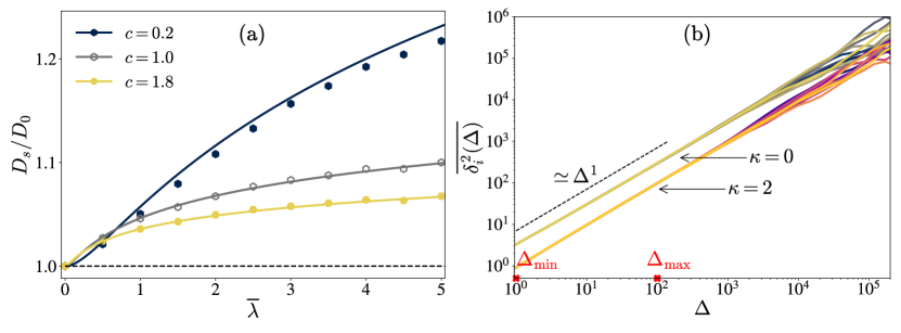
Figure 3: (a) Self-diffusion coefficient $D_{\mathrm{s}}/D_{0}$ as a function of the dimensionless coupling parameter $\overline{\lambda}$. The curves are computed with three different area fractions $c$, and with an oddness parameter $\kappa=2>\kappa_{c}$, such that we are in the enhancement regime and $D_{\mathrm{s}}>D_{0}$. (b) Typical TAMSD $\overline{\delta^{2}_{i}(\Delta)}$ curves as a function of lag-time $\Delta$ related to $i=1,\ldots,10$ trajectories of a total length of $T=4\times 10^{5}$ real-time steps in the case of $N=200$ interacting particles with density $c=0.1$ and $\kappa\in\{0,2\}$. The values $\Delta_{\mathrm{min}}=1$ and $\Delta_{\mathrm{max}}=100$ mark the interval of lag times $\Delta$ (in real-time units) used for ensemble averaging the TAMSDs.

The conservative force $\bi{F}_{i}(t)$ exerted on particle $i$ and appearing in Eq. (68) is given by the sum of pairwise interaction forces $\bi{F}_{i}(t)=\sum_{j=0}^{N}\bi{f}_{ij}(t)$, where $\bi{f}_{ij}$ derives from a (normalised) Gaussian interaction potential $\mathcal{U}$, i.e., $\bi{f}_{ij}=-\lambda\nabla\mathcal{U}(R_{ij})$ if $R_{ij}<\delta_{c}$ and $\bi{f}_{ij}=0$ if $R_{ij}>\delta_{c}$. Here, $R_{ij}=|\bi{X}_{i}(t)-\bi{X}_{j}(t)|$ is the inter-particle distance, and $\delta_{c}$ denotes a cut-off length scale that we use in order to truncate the interaction potential $\mathcal{U}(R_{ij})$ for reducing the computational time required by the Brownian dynamics simulations. In particular, if $\delta_{c}$ is sufficiently larger than the typical decay length of $\mathcal{U}(R_{ij})$, the error introduced by this truncation is negligible. For the Gaussian interaction potential reported in Eq. (33), we choose $\sigma=1.0$. Note that $\sigma$ is used as an effective particle radius, from where we deduce the effective concentration of particles $c=\pi\sigma^{2}\,N/L^{2}$, where $L$ is the length of the square simulation box. The cut-off distance of the interaction force is chosen to be $\delta_{c}=4\sigma$.

The dimensionless interaction scale $\overline{\lambda}=\lambda_{\mathrm{tr}}/(2\pi\sigma^{2}\,T)$ is given in terms of the coupling $\lambda_{\mathrm{tr}}$ compared with the thermal energy $T$ and the length scale $\sigma$ of the Gaussian potential. For a comparison between theoretical predictions and simulation results, see Fig. 3(a), where different couplings $\overline{\lambda}$ are tested. The analytical predictions are expected to be valid in a regime where the coupling between the tracer and the host particle is sufficiently small. However, from Fig. 3(a) it can be seen that at high densities ($c=1.0$ and $c=1.8$) the whole range of tested couplings produces very accurate results. At the low density $c=0.2$, instead, the mismatch between the analytical prediction and the numerical data increases upon increasing $\overline{\lambda}$. As a compromise between the accuracy of the analytical predictions and the magnitude of the effects shown in the figures of the main text (Section 3), we opt for $\overline{\lambda}=1$ and compare the results with $\overline{\lambda}=4$ in Fig. 2 of the main text. Note that $\overline{\lambda}=1$ is such that the maximum of the interaction energy $\overline{\lambda}\,\mathcal{U}(R_{ij})$ is equal to the thermal energy $T$.

To solve the first-order stochastic differential equation (68) we use the standard Euler-Maruyama scheme [22], where $\bi{X}_{i}(t_{n+1})$ and $\bi{V}_{i}(t_{n+1})$ are calculated from $\bi{X}_{i}(t_{n})$ and $\bi{V}_{i}(t_{n})$ and $t_{n+1}=t_{n}+\Delta t$ with $\Delta t=10^{-3}$. The thermal noise is accounted for by $\sqrt{2\gamma_{i}T\Delta t}\,\mathcal{N}(0,\mathbf{1})$, where $\mathcal{N}(0,\mathbf{1})$ is a two-dimensional random vector drawn from a multivariate normal distribution with zero mean and covariance matrix given by the identity matrix $\mathbf{1}$. Note that the discretised stochastic equations of motion are interpreted according to the Itô prescription, implying that the standard deviation of the noise is proportional to $\sqrt{\Delta t}$. To simulate Eq. (68) we use a square box of length $L$ with periodic boundary conditions, where the box length is determined so as to result into the desired density of particles $c$, i.e., $L=\sqrt{\pi\sigma^{2}N/c}$. As the interaction force does not diverge for $R_{ij}\rightarrow 0$ and particle overlaps are possible, we initialise the position of the $N=200$ particles according to a uniform distribution over the finite box. After an initial equilibration period of $n_{\mathrm{eq}}=10^{7}$ time steps, we start recording the stochastic trajectory for a total duration of $n_{\mathrm{tot}}=4\times 10^{8}$ time steps, which corresponds to a trajectory length of $T=4\times 10^{5}$ in real-time units. For an efficient computation, we used a neighbour-list implementation for the evaluation of the interaction forces, with a buffer radius $\delta_{\mathrm{buff}}$ which has been optimised in order to minimise the computational time. Over the broad range of densities simulated, a buffer-radius of $\delta_{\mathrm{buff}}\approx 2\delta_{c}$ turned out to be the most efficient.

D.2 MSD evaluation

In order to evaluate the diffusion coefficient of the tracer particle we calculate the time-averaged MSD (TAMSD) [111] for each (independent) trajectory $i$ according to

$$\overline{\delta^{2}_{i}(\Delta,T)}=\frac{1}{T-\Delta}\int_{0}^{T-\Delta}\mathrm{d}t\ |\bi{X}_{0}^{\{i\}}(t+\Delta)-\bi{X}_{0}^{\{i\}}(t)|^{2},$$ (69)

where $\bi{X}_{0}^{\{i\}}(t)$ is the the position of the tracer particle at time $t$ in trajectory $i$, $T$ is the trajectory length and $\Delta$ is the lag time. As the system under consideration is ergodic, we can ensemble-average over the $i=1,\ldots,i_{\mathrm{max}}$ independent trajectories to obtain the estimate for the MSD [112], which is formally defined as

$$\left\langle|\mathbf{X}_{0}(t)-\mathbf{X}_{0}(0)|^{2}\right\rangle =\lim_{T\to\infty}\left\langle\overline{\delta^{2}_{i}(\Delta=t,T)}\right\rangle$$ (70)

$$=\lim_{T\to\infty}\frac{1}{i_{\mathrm{max}}}\sum_{i=1}^{i_{\mathrm{max}}}\overline{\delta^{2}_{i}(t=\Delta,T)}.$$

By taking $T$ large enough one can assume that the initial conditions play no role in the evaluation of the long-time MSD. Hence, for the sake of simplicity, we impose $\mathbf{X}_{0}(t_{0})=\mathbf{0}$. We observe from Fig. 3(b) that the most reliable $\Delta$-range from which to extract the MSD is $1=\Delta_{\mathrm{min}}\leq\Delta\leq\Delta_{\mathrm{max}}=100$. The MSD is then used to deduce the self-diffusion coefficient $D_{\mathrm{s}}$ by fitting a linear time-dependence $\langle|\mathbf{X}_{0}(t)|^{2}\rangle=4\,D_{\mathrm{s}}\,t$, where we take $N_{\Delta}=40$ logarithmically equidistant lag-times to fit the MSD and ensemble average over $i_{\mathrm{max}}=10$ independent trajectories.

References

References

- [1] Höfling F and Franosch T 2013 Rep. Prog. Phys. 76 046602
- [2] Ramadurai S, Holt A, Krasnikov V, van den Bogaart G, Killian J A and Poolman B 2009 J. Am. Chem. Soc. 131 12650–12656
- [3] Scott S, Weiss M, Selhuber-Unkel C, Barooji Y F, Sabri A, Erler J T, Metzler R and Oddershede L B 2023 Phys. Chem. Chem. Phys. 25 1513–1537
- [4] Maxwell J C 1867 Philos. Trans. R. Soc. 49–88
- [5] Stefan J 1871 Sitzungsber. Kaiserl. Akad. Wiss. 63 63–124
- [6] Boltzmann L 1896 Vorlesungen über Gastheorie. 1. Theil: Theorie der Gase mit einatomigen Molekülen, deren Dimensionen gegen die mittlere Weglänge verschwinden (Verlag von Johannes Ambrosius Barth (Arthur Meiner)) URL https://www.deutschestextarchiv.de/boltzmann_gastheorie01_1896
- [7] Maxwell J C 1875 Nature 11 374–377
- [8] Hanna S, Hess W and Klein R 1982 Physica A 111 181–199
- [9] Imhof A and Dhont J K G 1995 Phys. Rev. E 52 6344
- [10] Felderhof B U and Jones R B 1983 Physica A 121 329–344
- [11] Löwen H and Szamel G 1993 J. Phys. Condens. Matter 5 2295
- [12] Kushick J and Berne B J 1973 J. Chem. Phys. 59 3732–3736
- [13] Bembenek S D and Szamel G 2000 J. Phys. Chem. B 104 10647–10652
- [14] Yamaguchi T, Matubayasi N and Nakahara M 2001 J. Chem. Phys. 115 422–432
- [15] Seefeldt K F and Solomon M J 2003 Phys. Rev. E 67 050402
- [16] Wensink H H, Löwen H, Rex M and Likos Christos N and van Teeffelen S 2008 Comp. Phys. Commun. 179 77–81
- [17] Krekelberg W P, Kumar T, Mittal J, Errington J R and Truskett T M 2009 Phys. Rev. E 79 031203
- [18] Weeks E R and Weitz D A 2002 Phys. Rev. Lett. 89 095704
- [19] Michailidou V, Petekidis G, Swan J and Brady J 2009 Phys. Rev. Lett. 102 068302
- [20] Peng Y, Chen W, Fischer T M, Weitz D A and Tong P 2009 J. Fluid Mech. 618 243–261
- [21] Thorneywork A L, Rozas R E, Dullens R P A and Horbach J 2015 Phys. Rev. Lett. 115 268301
- [22] Kalz E, Vuijk H D, Abdoli I, Sommer J U, Löwen H and Sharma A 2022 Phys. Rev. Lett. 129 090601
- [23] Hargus C, Epstein J M and Mandadapu K K 2021 Phys. Rev. Lett. 127 178001
- [24] Langer A, Sharma A, Metzler R and Kalz E 2024 Phys. Rev. Res. 6(4) 043036
- [25] Kalz E, Vuijk H D, Sommer J U, Metzler R and Sharma A 2024 Phys. Rev. Lett. 132 057102
- [26] Kurşunoǧlu B 1962 Ann. Phys. 17 259–268
- [27] Karmeshu 1974 Phys. Fluids 17 1828–1830
- [28] Chun H M, Durang X and Noh J D 2018 Phys. Rev. E 97 032117
- [29] Park J M and Park H 2021 Phys. Rev. Res. 3 043005
- [30] Muzzeddu P L, Vuijk H D, Löwen H, Sommer J U and Sharma A 2022 J. Chem. Phys. 157 134902
- [31] Chan C W, Wu D, Qiao K, Fong K L, Yang Z, Han Y and Zhang R 2024 Nat. Commun. 15 1406
- [32] Kalz E, Sharma A and Metzler R 2024 J. Phys. A 57 265002
- [33] Valecha B, Muzzeddu P L, Sommer J U and Sharma A 2024 arXiv:2409.18703
- [34] Koch D L and Brady J F 1987 Phys. Fluids 30 642650
- [35] Auriault J L, Moyne C and Amaral Souto H P 2010 Transport Porous Med. 85 771–783
- [36] Ghimenti F, Berthier L, Szamel G and van Wijland F 2024 Phys. Rev. E 110 034604
- [37] Ghimenti F, Berthier L, Szamel G and van Wijland F 2023 Phys. Rev. Lett. 131(25) 257101
- [38] Brown B L, Täuber U C and Pleimling M 2018 Phys. Rev. B 97 020405(R)
- [39] Gruber R, Brems M A, Rothörl J, Sparmann T, Schmitt M, Kononenko I, Kammerbauer F, Syskaki M A, Farago O, Virnau P and Kläui M 2023 Adv. Mater. 35 2208922
- [40] Schick D, Weißenhofer M, Rózsa L, Rothörl J, Virnau P and Nowak U 2024 Phys. Rev. Res. 6 013097
- [41] Wu P, Huang R, Tischer C, Jonas A and Florin E L 2009 Phys. Rev. Lett. 103 108101
- [42] Volpe G, Maragò O M, Rubinsztein-Dunlop H, Pesce G, Stilgoe A B et al. 2023 J. Phys. Photonics 5 022501
- [43] Reichhardt C J O and Reichhardt C 2022 Europhys. Lett. 137 66004
- [44] Cao X, Das D, Windbacher N, Ginot F, Krüger M and Bechinger C 2023 Nat. Phys. 19 1904–1909
- [45] Shalchi A 2011 Phys. Rev. E 83 046402
- [46] Effenberger F, Fichtner H, Scherer K, Barra S, Kleimann J and Strauss R D T 2012 Astrophys. J. 750 108
- [47] Likos C N 2001 Phys. Rep. 348 267–439
- [48] Vlassopoulos D and Cloitre M 2014 Curr. Opin. Colloid Interface Sci. 19 561–574
- [49] Stillinger F H 1976 J. Chem. Phys. 65 3968–3974
- [50] Stillinger F H and Weber T A 1978 J. Chem. Phys. 68 3837–3844
- [51] Stillinger F H 1979 J. Chem. Phys. 70 4067–4075
- [52] Stillinger F H 1979 Phys. Rev. B 20 299
- [53] Stillinger F H and Weber T A 1980 Phys. Rev. B 22 3790
- [54] Weber T A and Stillinger F H 1981 J. Chem. Phys. 74 4020–4028
- [55] Flory P J and Krigbaum W R 1950 J. Chem. Phys. 18 1086–1094
- [56] Louis A A, Finken R and Hansen J P 1999 Europhys. Lett. 46 741
- [57] Lang A, Likos C N, Watzlawek M and Löwen H 2000 J. Phys. Condens. Matter 12 5087
- [58] Likos C N, Lang A, Watzlawek M and Löwen H 2001 Phys. Rev. E 63 031206
- [59] Bolhuis P G, Louis A A, Hansen J P and Meijer E J 2001 J. Chem. Phys. 114 4296–4311
- [60] Louis A A, Bolhuis P G, Hansen J P and Meijer E J 2000 Phys. Rev. Lett. 85(12) 2522–2525
- [61] Bolhuis P G and Louis A A 2002 Macromolecules 35 1860–1869
- [62] Likos C N, Schmidt M, Löwen H, Ballauff M, Pötschke D and Lindner P 2001 Macromolecules 34 2914–2920
- [63] Stillinger F H and Stillinger D K 1997 Physica A 244 358–369
- [64] Mausbach P and May H O 2006 Fluid Ph. Equilib. 249 17–23
- [65] Mausbach P and May H O 2009 Z. Phys. Chem. 223 1035–1046
- [66] Shall L A and Egorov S A 2010 J. Chem. Phys. 132
- [67] Speranza C, Prestipino S and Giaquinta P V 2011 Mol. Phys. 109 3001–3013
- [68] Archer A J 2003 Statistical mechanics of soft core fluid mixtures Ph.D. thesis University of Bristol
- [69] Sposini V, Likos C N and Camargo M 2023 Soft Matter 19 9531–9540
- [70] Prestipino S, Saija F and Giaquinta P V 2011 Phys. Rev. Lett. 106 235701
- [71] Mendoza-Coto A, Mattiello V, Cenci R, Defenu N and Nicolao L 2024 Phys. Rev. B 109 064101
- [72] Dean D S 1996 J. Phys. A 29 L613
- [73] Kawasaki K 1994 Physica A 208 35–64
- [74] Illien P 2024 arXiv:2411.13467
- [75] Benois A, Jardat M, Dahirel V, Démery V, Agudo-Canalejo J, Golestanian R and Illien P 2023 Phys. Rev. E 108 054606
- [76] Jardat M, Dahirel V and Illien P 2022 Phys. Rev. E 106 064608
- [77] Marbach S, Dean D S and Bocquet L 2018 Nat. Phys. 14 1108–1113
- [78] Wang Y, Dean D S, Marbach S and Zakine R 2023 J. Fluid Mech. 972 A8
- [79] Vuijk H D, Brader J M and Sharma A 2019 J. Stat. Mech.: Theory Exp. 2019 063203
- [80] Démery V, Bénichou O and Jacquin H 2014 New J. Phys. 16 053032
- [81] Poncet A, Bénichou O, Démery V and Oshanin G 2017 Phys. Rev. Lett. 118 118002
- [82] Venturelli D, Illien P, Grabsch A and Bénichou O 2024 arXiv:2411.09326
- [83] Täuber U C 2014 Critical Dynamics: A Field Theory Approach to Equilibrium and Non-Equilibrium Scaling Behavior (Cambridge University Press)
- [84] Venturelli D, Ferraro F and Gambassi A 2022 Phys. Rev. E 105 054125
- [85] Venturelli D and Gambassi A 2022 Phys. Rev. E 106 044112
- [86] Venturelli D and Gambassi A 2023 New J. Phys. 25 093025
- [87] Venturelli D, Loos S A M, Walter B, Roldán É and Gambassi A 2024 Europhys. Lett. 146 27001
- [88] Basu U, Démery V and Gambassi A 2022 SciPost Phys. 13 078
- [89] Démery V and Dean D S 2011 Phys. Rev. E 84 011148
- [90] Démery V and Fodor É 2019 J. Stat. Mech.: Theory Exp. 2019 033202
- [91] Démery V and Gambassi A 2023 Phys. Rev. E 108 044604
- [92] Pond M J, Krekelberg W P, Shen V K, Errington J R and Truskett T M 2009 J. Chem. Phys. 131
- [93] Pond M J, Errington J R and Truskett T M 2011 J. Chem. Phys. 134
- [94] Nakamura T and Yoshimori A 2009 J. Phys. A 42 065001
- [95] Durán-Olivencia M A, Yatsyshin P, Goddard B D and Kalliadasis S 2017 New J. Phys. 19 123022
- [96] Archer A J and Evans R 2001 Phys. Rev. E 64 041501
- [97] Louis A A, Bolhuis P G and Hansen J P 2000 Phys. Rev. E 62 7961
- [98] Hertlein C, Helden L, Gambassi A, Dietrich S and Bechinger C 2008 Nature 451 172–175
- [99] Gambassi A, Maciołek A, Hertlein C, Nellen U, Helden L, Bechinger C and Dietrich S 2009 Phys. Rev. E 80 061143
- [100] Martínez I A, Devailly C, Petrosyan A and Ciliberto S 2017 Entropy 19 77
- [101] Magazzu A, Callegari A, Staforelli J P, Gambassi A, Dietrich S and Volpe G 2019 Soft Matter 15 2152–2162
- [102] Gambassi A and Dietrich S 2024 Soft Matter 20 3212–3242
- [103] Kuroda Y and Miyazaki K 2023 J. Stat. Mech.: Theory Exp. 2023 103203
- [104] Fruchart M, Scheibner C and Vitelli V 2023 Annu. Rev. Condens. Matter Phys. 14 471–510
- [105] Reichhardt C and Reichhardt C J O 2019 Phys. Rev. E 100 012604
- [106] Yang Q, Zhu H, Liu P, Liu R, Shi Q, Chen K, Zheng N, Ye F and Yang M 2021 Phys. Rev. Lett. 126 198001
- [107] Poggioli A R and Limmer D T 2023 Phys. Rev. Lett. 130 158201
- [108] Hosaka Y, Golestanian R and Daddi-Moussa-Ider A 2023 New J. Phys. 25 083046
- [109] Duclut C, Bo S, Lier R, Armas J, Surówka P and Jülicher F 2024 Phys. Rev. E 109 044126
- [110] Lier R, Duclut C, Bo S, Armas J, Jülicher F and Surówka P 2023 Phys. Rev. E 108 L023101
- [111] He Y, Burov S, Metzler R and Barkai E 2008 Phys. Rev. Lett. 101 058101
- [112] Burov S, Jeon J H, Metzler R and Barkai E 2011 Phys. Chem. Chem. Phys. 13 1800–1812