TESSELLATE: Piecing Together the Variable Sky With TESS

Abstract

We present TESSELLATE, a dedicated pipeline for performing an untargeted search documenting all variable phenomena captured by the TESS space telescope. Building on the TESSreduce difference imaging pipeline, TESSELLATE extracts calibrated and reduced photometric data for every full frame image in the TESS archive. Using this data, we systematically identify transient, variable and non-sidereal signals across timescales ranging from minutes to weeks. The high cadence and wide field of view of TESS enables us to conduct a comprehensive search of the entire sky to a depth of $\sim$17$\;m_{i}$. Based on the volumetric rates for known fast transients, we expect there to be numerous Fast Blue Optical Transients and Gamma Ray Burst afterglows present in the existing TESS dataset. Beyond transients, TESSELLATE can also identify new variable stars and exoplanet candidates, and recover known asteroids. We classify events using machine learning techniques and the work of citizen scientists via the Zooniverse Cosmic Cataclysms project. Finally, we introduce the TESSELLATE Sky Survey: a complete, open catalog of the variable sky observed by TESS.

1 Introduction

The Transiting Exoplanet Survey Satellite (TESS, Ricker et al., 2014) has imaged nearly the entire sky in the near-infrared since starting operations in late 2018. Its wide field of view (FoV) of $2160\rm\,deg^{2}$ and its continuous, high-cadence observation strategy have allowed TESS to fill a niche role in the transient community. While initially designed to hunt for exoplanets in the Milky Way, its science use has since expanded widely, including the study of variable stars (Bruch, 2022; Liu & Qian, 2023; Fetherolf et al., 2023), supernovae (SNe, Fausnaugh et al., 2021; Vallely et al., 2021; Fausnaugh et al., 2023; Wang et al., 2023, 2024), gamma-ray burst (GRB) afterglows (Smith et al., 2021; Fausnaugh et al., 2023; Roxburgh et al., 2023; Jayaraman et al., 2024), asteroids (Pál et al., 2018, 2020; Woods et al., 2021; McNeill et al., 2023), comets (Ridden-Harper et al., 2021a; Farnham et al., 2021), exocomets (Zieba et al., 2019; Dobrycheva et al., 2023), stellar flares (Günther et al., 2020; Pietras et al., 2022), and other transient phenomena.

As the TESS mission has evolved, the volume of data produced from each target field, known as a TESS ‘sector’, has greatly increased. Upon launch, it captured full-frame images (FFIs) at a cadence of 30 minutes; this interval was reduced to 10 minutes between 5^th July 2020 – 31^st August 2022, and has since been further shortened to just 200 seconds.

The data from each sector is released to the public through the MAST archive as a time-series of FFIs that are ‘calibrated’ but not background subtracted. As such, observers are required to perform their own photometric extraction for sources that are not automatically extracted through the SPOC pipeline (Caldwell et al., 2020). There are a number of successful reduction pipelines available to the public (e.g. Ridden-Harper et al., 2021b; Fausnaugh et al., 2021; Feinstein et al., 2020), each with advantages and disadvantages due to their choice of techniques. However, these pipelines are often small-scale, focusing on producing cutouts of TESS data around desired coordinates or sources. This means that captured information has been left unexamined in the gaps between targeted searches.

With TESS’s past success as a transient hunter across many time-domain fields, the motivation for a complete archival search of its images is clear. In particular, TESS is expected to be a powerful tool for observing fast extragalactic transients such as orphan GRB afterglows (Freeburn et al., 2024; Perley et al., 2025). Such events evolve on timescales of minutes to hours; the combination of TESS’s wide field of view and rapid temporal resolution make it capable of discovering and sampling fast events at high time resolution.

In this paper, we introduce TESSELLATE: the TESS Extensive Lightcurve Logging and Analysis of Transient Events pipeline, the first system capable of automatically searching every TESS frame to document all fast transient events captured by TESS. For this pipeline, we use TESSreduce to remove the scattered light background and create difference images. TESSELLATE is purpose-built for use on the OzSTAR supercomputing node held at Swinburne University, and is wrapped in a user-friendly python package that allows for simple but thorough control of the various processing steps.

We developed TESSELLATE to be agnostic of transient type, allowing it to detect a wide range of variable, transient and non-sidereal phenomena. Figure 1 shows an example difference image with detections and an array of assorted event detections. In this paper, all magnitudes are assumed to be AB unless stated otherwise, and magnitudes in TESS are represented by $m_{T}$. Furthermore, we take $m_{i}\approx m_{T}$ for stellar spectral energy distributions, where $m_{i}$ is the apparent $i$ band magnitude. Section 2 describes each stage of the pipeline; Section 3.1 provides detection efficiency estimates for a selection of TESS sectors; Section 4 highlights a variety of science cases to which TESSELLATE can be applied. Finally, Section 5 outlines the TESSELLATE Sky Survey made using TESSELATE, and how its data products are delivered.

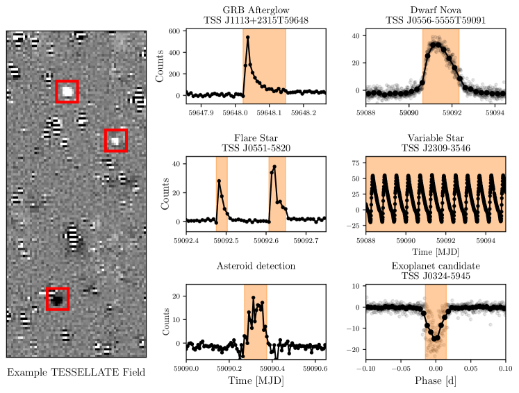
Figure 1: Event identification from TESS images with TESSELLATE. Left: Example image section that has been background subtracted and differenced. Sources identified with TESSELLATE are indicated with red boxes. Center & Right: Example TESS light curves with events detected by TESSELLATE highlighted. For the recovered exoplanet (lower right) we show the phase-folded light curve with raw data (gray) and 10 minute binned light curve (black). Similarly for the dwarf nova (top right) we show the raw data (gray) and 6 hour binned light curve (black). The asteroid detection (lower left) shows an individual detection at a position on the detector and time.

2 Pipeline Overview

The TESSELLATE pipeline runs a full reduction and transient event extraction process on individual TESS sectors, simultaneously operating on all 16 CCDs from the 4 cameras of TESS. This pipeline is built upon the process described in Roxburgh et al. (2023) to conduct an untargeted transient search. When executed, TESSELLATE calls sub-processes sequentially, as visualized in Figure 2.

We tested TESSELLATE using data from Sector 29, which observed from August 26^th to September 21^st 2020. This southern-pointing sector used the intermediate FFI cadence of 10 minutes and has significant complementary coverage with the DECam Local Volume Exploration Survey (DELVE, Drlica-Wagner et al., 2021).

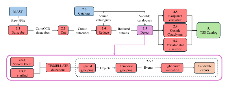
Figure 2: Schematic of the TESSELLATE pipeline. The detection workflow is expanded upon in the purple box. The section relevant to each step is indicated by the number at the top of the boxes.

2.1 TESS Datacube Generation

We acquire all TESS FFI data from the MAST archive. A full TESS image is constructed from four cameras with four CCDs. Each of the 16 CCDs form a 2048$\times$2048 pixel array with an angular resolution of 21” per pixel. Files are saved into hierarchical file structures based on the sector and camera information.

For each of the 16 CCDs, the FFIs are collated into three-dimensional datacubes termed ‘Target Pixel Files’ (TPFs) using astrocut (Brasseur et al., 2019). For sectors in the second extended mission, i.e. those with FFIs captured every 200 seconds, a single TPF datacube exceeds 300 GB. While they can be generated in this form, we divide these sectors into two datacubes. This split is made at the downlink time in TESS’s orbit, which generally occurs near the halfway mark of the time series but can vary by a week either side.

2.2 Cutting Datacubes

In this stage, each of the generated datacubes are further divided into a number of cutouts, also completed using the astrocut package. This division enables further parallel processing and decreases the size of individual reduction tasks. Furthermore, the TESSreduce package produces more reliable subtractions of the scattered light background for smaller regions with less dynamic range in the background. The number of cutouts is adjustable; by default each datacube is divided into 16 equal cutouts of $512\times 512\;$pixels.

2.3 Catalog Acquisition

TESSELLATE gathers a number of external source catalogs to be used in data reduction and source identification. Most catalogs are accessed through Vizier queries made using astroquery (Ginsburg et al., 2019). For a given cutout, each query is centered on the central coordinates of the cutout, with a radius to fully cover the cuts.

The reduction stage requires a source catalog to generate a source mask for image alignment. We use Gaia DR3 as the source catalog due to its complete coverage of the sky to magnitudes $>19\;G_{\rm mag}$.

To assist in object identification during the detection stage, TESSELLATE builds a unified variable star catalog from several catalogs: the Gaia DR3 variability catalog (Eyer et al., 2023) (I/358/varisum), DES RRyrae catalog (Stringer et al., 2019) (J/AJ/158/16/table11), ASAS-SN variable star catalog Jayasinghe et al. (2018), and ATLAS-VAR catalog (Heinze et al., 2018). The ATLAS-VAR catalog is accessed through MAST using the mastcasjobs package. In the final joined catalog, we consider sources to be duplicates if they are within 2″ and only retain the first instance.

2.4 Cutout Reduction

All cutouts are reduced using the TESSreduce package for python. This involves all the processing steps required to extract accurate photometry from TESS data: background modeling and subtraction, image alignment, and flux calibration, as described by (Ridden-Harper et al., 2021b). A few of the more rigorous steps normally applied by TESSreduce are omitted to reduce compute time, such as the secondary background correlation correction. This process produces a difference-imaged datacube, where static sources are subtracted. We show a result of this reduction process in Figure 1 (left). Additionally, we save output diagnostic files, including the calculated scattered light background, position offsets, and the reference image used in subtraction.

2.5 Transient Event Search & Isolation

The core of TESSELLATE is the detection and identification of events. The components of this source detection process are discussed in the following subsections. The low spatial resolution of TESS and artifacts from the scattered light background present challenges to reliably detect real sources while minimizing false detections. Detecting faint sources becomes particularly challenging as sources may only have significant flux in $\sim$3 pixels. For the detection process, we developed a two-stage process that uses information from individual differenced images in the first stage, and resultant event light curves for the second stage.

To maximize source detection in the first stage, we have developed two independent source detection pipelines. The first pipeline, SourceDetect, utilizes machine learning techniques to identify sources in images (§ 2.5.1), while the second pipeline uses conventional source detection (§ 2.5.2). These two methods rely on the effective PSF (ePSF) model for TESS, which is obtained through the TESS_PRF package (Bell & Higgins, 2022). Both methods are capable of detecting decreases and increases in flux which we refer to as negative and positive detections, respectively. This process allows us to identify transients, variable stars, exoplanet transits, and any other phenomena that changes the source brightness.

In the second stage we isolate spatially co-located detections into “objects”, which are then temporally isolated into “events”. This source detection process is agnostic of light curve shape, or object type. All detections are recorded and quality cuts applied in post-processing stages.

2.5.1 SourceDetect

The size and complexity of astronomical datasets have seen huge growth in recent years due to the deployment of large-scale surveys such as ZTF (Bellm et al., 2019), PS1 (Chambers et al., 2016), ATLAS (Tonry, 2011), and TESS. Such changes have required astronomers to develop automated tools to analyze these datasets. Machine learning algorithms are arguably the most popular example of innovations in this area and have already been applied to areas such as detection and classification (e.g. Baron, 2019). SourceDetect is a novel object detection method that searches for transient and variable star events. It employs a trained convolutional neural network (CNN, Hinton & Salakhutdinov, 2006; Benigo, 2009; LeCun et al., 2015) to identify candidate “PSF-like” events within TESS images or image cutouts of any shape.

The SourceDetect CNN was designed to identify both positive and negative-flux events and to differentiate between them and false objects such as overexposed regions or background artifacts. In the CNN architecture, nine parameters are extracted per detection: the likelihood that it is a real event, its dimensions, its pixel position, and its associated probability for four object classes. These classes are positive detections, negative detections, and two representing false objects such as background artifacts. The model was trained and tested using a dataset of 12,800, $16\times 16$ pixel images with a background generated from a Gaussian distribution to mimic the real reduced TESS images. Each image contained up to two objects from the four classes with varying brightnesses and pixel positions. Further details on SourceDetect will be presented in (Moore et al., in prep.).

2.5.2 Starfind

In addition to SourceDetect, we use conventional source finding methods using the TESS_PRF effective TESS PSF. The Starfind source detection method relies on the photutils (Bradley et al., 2024) starfind algorithm. With starfind, a kernel can be specified to represent the ePSF of sources in the image. We apply this detection method to every frame in the TESS sector.

As the TESS ePSF is under-sampled, the shape changes significantly under sub-pixel shifts. To account for the variety of appearances for the ePSF we run starfind five times with kernels that correspond to a perfectly centered source, then sources shifted by 0.25 pixels in x and y for each corner. While this combination of sources will not perfectly represent all possible TESS ePSF configurations, it is effective at identifying sources. We compress the results from the 5 searches into a single dataframe, dropping co-located duplicates.

At the detection stage we aim to identify all possible sources, so a low detection threshold of just 2$\sigma$ above the background is set. We remove obvious bad detections by cutting all detections with reported FWHM less than 0.8 and greater than 7 pixels. These FWHM cuts are effective at removing cosmic rays, and broad features, such as a region of poorly subtracted background. We also add a further cut on the standard deviation of the background as calculated by the TESSreduce reduction at the location of the detection. This check on the background limits contamination from poor scattered light subtractions.

This starfinding detection method outputs a dataframe similar to that produced by SourceDetect. If both SourceDetect and starfind are run on the data, as is default in TESSELLATE, the two dataframes are joined, retaining only the first instance of detections that are spatially located and occur in the same frame.

2.5.3 Event Isolation

Following the detection of point sources in each TESS FFI, we then group sources into spatially co-located “objects”, which can then have temporally continuous “events” associated with them. For each object, we consider negative and positive detections independently to create negative and positive events. As each event is separated we are able to identify and analyze independent events, such as multiple stellar flares (e.g. Figure 1 flare star example), or identify individual peaks and troughs of variable stars.

Detections are grouped spatially using the DBscan clustering algorithm through the scikit-learn package (Pedregosa et al., 2011), implemented with a minimum sample number of 1 and $\rm eps=0.5$. Each object is assigned a unique ID, and is then parsed through time to isolate temporally independent events. This process builds on the method used in the Kepler/K2: Background Survey (Ridden-Harper et al., 2020), where consecutive detections are considered as a single event. To limit random noise and missing detections breaking up continuous events we consider two independent detections to be of the same event, if there are fewer than 5 non-detection frames between them. While we record all detections, we require “events” to be constructed from 2 or more consecutive detections to limit contamination from cosmic rays. As we treat positive and negative flux triggers independently, we obtain a series of events that cover each maxima and minima of the light curve.

The times and durations of these events are refined through analysis of their light curves; in many cases, the undersampled ePSF of TESS is susceptible to being obscured by noise, while the cumulative signal in the light curve often remains significant. For each spatially resolved object, we extract light curves using the circle aperture method implemented in photutils, with a 1.5 pixel radius. We calculate a “significance light curve” by subtracting the local mean - 24 hours plus a buffer either side of the event - and then dividing by the standard deviation of the light curve near to the event. This buffer is set to half the duration of the event, defined to avoid biasing the light curve statistics with parts of the event which are not included in the preliminary event times. With the significance light curve for each event, we can identify accurate start and end times, which we consider to be when the event signal exceeds and returns within 3$\sigma$ of the median respectively. This refines the event times such that they fully encompass the interval within which the light curve exhibits significant flux.

We also use the significance light curve to define two additional detection quality metrics: the maximum and median significances of the light curve during the event. As the significance is calculated from the light curve near to the events, these metrics provide a means of removing spurious detections that are not statistically significant in the light curve, despite being identified from the images.

At the end of this, all events are collated into a single catalog. Coordinates are calculated at the object level from an average weighted by the detection significance, and are then crossmatched against the variable star catalog described in § 2.3. If the object is within 10″ of a source, they are assigned a “Type” taken from the catalogs. This type applies to all events that correspond to an object. For each object we also use Lomb-Scargle periodograms, as implemented in scipy to identify prominent frequencies and their power in the light curve.

At the end of this process we have a data frame containing all independent events and key parameters which can be used for event filtering. For each event we save the pipeline light curve, and generate figures to be used in § 2.9.

2.6 Targeted Search Functionality

While the primary pipeline workflow is designed as an untargeted survey, there are situations where it is beneficial to incorporate functionality for targeted searches as well. These can include attempts at cross-matching with known uncertainty regions of particular astrophysical events, such as gravitational wave detections or GRBs. As full TESSELLATE runs can be highly resource consuming, as outlined in § 2.10, it is convenient to quickly process smaller regions of interest.

To address this, we include an alternative TESSELLATE operational mode that allows for targeted observation of a known event. Taking an estimated coordinate, an associated one dimensional position uncertainty, and a time onset for the event, the pipeline determines its overlap with TESS imaging. If an overlap is found, the pipeline is called to process only the relevant sector and camera/CCD combinations.

Once the run is complete, three parameters are required: the maximum time duration of the transient, the maximum time delay between the initial event time and the event onset in TESS (to account for delays between emission mechanisms e.g. the gamma-ray emission and optical afterglow of GRBs), and a minimum light curve significance above the local median. The light curves and information of the brightest events that meet all the criteria will then be returned.

Figure 3 displays an example of this mode applied to the coordinates of the known TESS detection of GRB180807A. This shows the most significant event that coincides temporally and occurs within the GRB’s uncertainty region as reported by the Fermi space telescope. The left panel row presents the event’s light curve with respect to the GRB’s reported onset time in blue. The middle panel displays the CCD upon which the candidate was found (whose location is marked by the blue star), with the red grid representing the borders of each cutout; cutouts having overlap with the black localization region of the GRB are shaded. The right panel presents the brightest frame of the event.

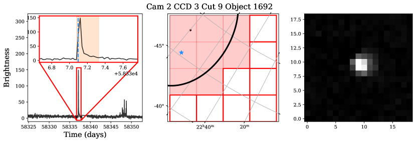
Figure 3: Targeted search for an optical counterpart to GRB180807A. Left: Event light curve for the detected event with the red insert zooming in on the detected transient. The transient is highlighted by the orange shaded region and the input trigger time is shown with the blue dashed line. Center: Plot of the spatial search area, where the central coordinates and uncertainty are shown with a black point and black line, respectively. Cuts of the TESS CCD that lie within the error region and are searched are highlighted in red, with the blue star representing the detected candidate. Right: Cutout of the difference image at the brightest point of the detected transient.

2.7 Candidate Selection

With TESSELLATE we can search all TESS data through both targeted and untargeted searches. Up to this point TESSELLATE uses a relaxed detection criteria to maximize detections of faint events. All detections are saved, and used to identify individual events. However, this process results in a large number of false detections which we then cut by imposing quality restrictions.

The main quality criteria include: image detection significance, light curve significance, flux sign of the event, event type, and standard deviation of the background. These options allow for high degrees of specification in the returned events, and can be chosen such that contamination is minimal.

For the general transient search we require that the event:

• is not matched to, or classified as a variable star,

• has an increase in flux,

• has an image significance greater than 2.5$\sigma$,

• has a mean light curve significance greater than 2.5$\sigma$,

• the standard deviation of the background of the calculated background at the position of the event is less than 50 counts.

These conditions reject most false positives while preserving faint events. The resulting sample can be cleaned of the remaining false positives through manual vetting. If stricter conditions, such as an increase in the signal significance are imposed, then contamination fraction becomes minimal at the expense of cutting faint events. Exoplanet candidates are identified through a similar procedure; however, the flux sign must be negative and the event duration must be less than a day.

2.8 Identifying Exoplanet Candidates

Since TESSELLATE can detect negative events, it can detect exoplanet candidates through dips in their light curves. As transits have expected shapes, they are readily disentangled from other events. We have augmented TESSELLATE with a post-processing pipeline to identify exoplanet candidates. This pipeline identifies negative events, and alters the light curve by flattening and normalizing it to the reference image counts. It then inspects transit characteristics such as depth and duration. We apply quality cuts on parameters such as signal-to-noise, the number of transits detected, and source crowding.

For each sector we run the exoplanet pipeline to identify all possible exoplanet candidates which then enter the planet vetting process. We fit the transits for each candidate transit with a simple parabolic model, filtering out candidates with low $\chi^{2}$ values. This step removes obvious outliers, such as detections of spurious noise. Furthermore, the processed light curve must still have a significant event at the times identified by TESSELLATE. We then identify the primary period and phase-fold the light curve.

We compute preliminary classifications for each phase-folded light curve with TRICERATOPS (Giacalone & Dressing, 2020; Giacalone et al., 2021). This pipeline identifies the best-fitting transit model from a suite of possible models, covering types of eclipsing binaries and exoplanet transits. Alongside light curve information, TRICERATOPS uses stellar parameters from the TESS Input Catalog and assess the potential impact of nearby sources. Candidates which are assigned high probability of being exoplanets are taken as TESSELLATE exoplanet candidates.

2.9 Cosmic Cataclysms: Citizen Science with Zooniverse

The enormous data volume of TESS produces tens of thousands of candidates per sector. While most false positives are removed by our triage steps, manual vetting is required for faint candidates. To produce a clean set of transients detected by TESSELLATE we have created the Cosmic Cataclysms citizen science project, hosted by Zooniverse. Zooniverse has hosted a wide variety of projects, and has been highly successful for transient searches such as the ‘Supernova Hunters’ project to detect supernovae observed by the Pan-STARRS 1.8m telescope (Fulton et al., 2020).

In Cosmic Cataclysms, citizen scientists are asked to classify transient candidates based on figures such as Figure 4. These figures contain the TESS light curve with the event detected by TESSELLATE highlighted in orange in the insert panel. We also include images showing the brightest frame centered on the event and another frame 1 hour later to identify movement of the source that might indicate that the event is an asteroid. Classifications by the citizen scientists are taken as a clean sample.

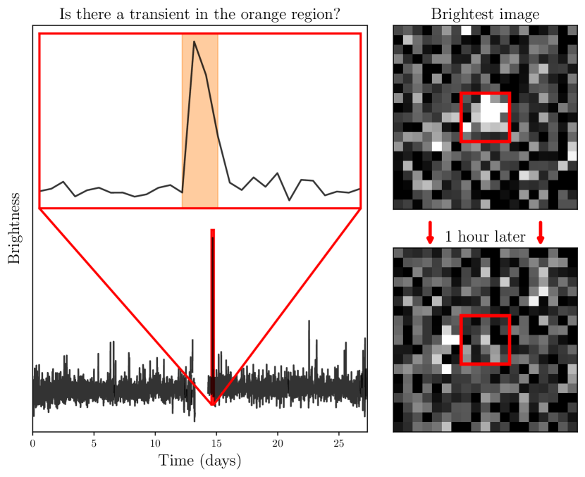
Figure 4: An example of a plot provided to the citizen scientists on Zooniverse. The upper-left shows a zoomed-in section of the difference image from the TESS light curve (lower-left). The upper-right displays an image from the brightest frame around the detected source, while the lower-right panel shows the frame one hour after the brightest observation. With this information citizen scientists are asked to classify the target.

2.10 Computational Resources

The TESSELLATE pipeline is designed to operate on SLURM based computational servers; we are primarily using the OzSTAR supercomputing node at Swinburne University. Each TESS sector is batched individually, with the primary processing steps spanning § 2.1 to § 2.5.3 all utilizing a single Standard Computer node with 32 cores. Each sub-process is initialized with memory and runtime limits specific to the task and sector; Table 1 displays the average requirements for 10 minute cadence data processing. These values are reduced for the 30 minute cadence data, and effectively doubled for the 200 second cadence data. As TESSELLATE has been constructed to be highly parallelized, multiple cuts are processed simultaneously.

Table 1: Average processing requirements for a 10 minute cadence sector for TESSELLATE sub-processes as deployed on an OzSTAR Standard Computer node with 32 cores. The data reduction and event detection steps run independently for each cut, so here we list the memory requirement to process a single cut. We exclude the time required for downloading the TESS data.

Sub-process	Memory (GB)	CCD runtime (CPU hours)	Sector runtime (CPU hours)
Cube Data	120	30	510
Cut Cubes	30	20	256
Data Reduction	110	770	12300
Event Detection	60	260	4100

3 Detection efficiency and event rates

3.1 Detection Efficiency

Understanding the detection efficiency of TESSELLATE is crucial for calculating its expected detection rate of real events. To this end, we inject simulated sources into the datacubes and compute recovery rates for each of TESS’s cameras. These sources are generated by TESS_PRF to match the variable ePSF of TESS, and are randomly assigned an $(x,y)$ position on the detector (at least 3 pixels from the image boundaries), a frame number between 0 and the total number of frames, and a brightness. The brightness is drawn from a log-uniform sample, ranging from 375 to 1.5 TESS counts; using the average TESS zeropoint of 20.44 (Vanderspek et al., 2018), this corresponds to an $m_{T}$ of between $14$ and $20$. We apply both detection methods independently, which allows us to compare their detection efficiencies.

The recovery rates for our test data for Sector 29 are shown in Figure 5. From both methods we have high recovery rates for all cameras until $\sim 17\;m_{T}$ at which point the recovery rate declines significantly. This decline coincides with a source brightness equivalent to a signal to noise ratio $<3$ when considering the average background. As the noise profile is not uniform across cuts, faint sources are only recoverable in areas with low noise.

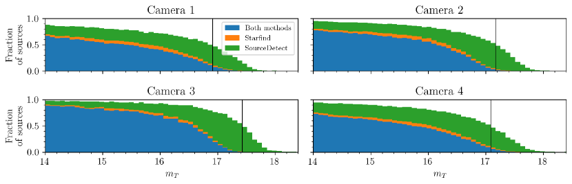
Figure 5: Mean recovery rates for the cameras in Sector 29. The recovered sources are flagged by their detection methods (Starfind and SourceDetect). The black line indicates the magnitude at which the recovery rate drops below 50% for each camera.

From Sector 29 we find that the cameras and CCDs are largely consistent in their recovery rates. The recovery rate depends on our ability to reliably model and subtract the scattered light background. This becomes particularly challenging for cameras with highly dynamic source scattered light backgrounds and crowding, such as cameras near the ecliptic and galactic plane. We see the impact of the scattered light background in Figure 5 where Camera 1 has a significantly worse recovery rate for all sources when compared to the cameras further from the ecliptic.

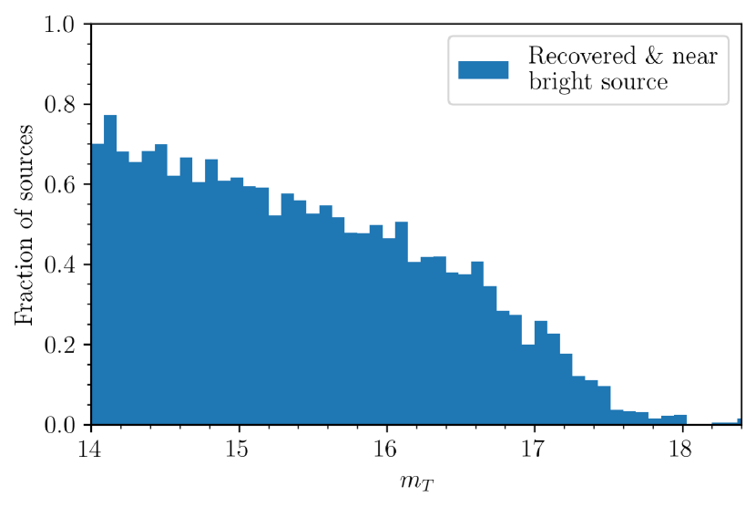
Figure 6: Mean recovery rates across Sector 29 of ePSFs injected within a one pixel radius of a bright source. These are flagged using the TESSELLATE source mask.

Source recovery is also limited by subtraction artifacts. Poorly subtracted bright sources can leave complex residuals which can obscure even bright injected events. Examples of these residuals can be seen in Figure 1 (left) which are often characterized by a checkerboard pattern of positive and negative fluxes. For Sector 29 we find that $\sim$20% of all injected sources are considered to be close to bright sources. In Figure 6 we show the recovery rate of the $\sim$20% of sources that were injected near a bright source. While it is clear that subtraction artifacts impact the recoverability of all sources, sources fainter than $16\;m_{T}$ are significantly impacted.

The results of our efficiency trials are consistent with other work, although in some instances our detection threshold is brighter. Fausnaugh et al. (2023) found that GRB230307A was undetectable when it reached a magnitude fainter than $m_{T}>17.79$. While TESSELLATE is able to recover sources to equivalent depths, the low recovery efficiency suggests that there may be room to improve sensitivity in our pipeline.

3.2 Event Rates

With these detection efficiencies, we can make estimates for the expected number of individual events of known transient classes that have been observed by TESS and will be recovered by TESSELLATE. For this rate estimation we use the average recovery rate from all cameras in Sector 29 and assume it to be representative of all sectors. While TESS has three distinctive observing cadences, we do not see significant changes in recovery rate tests between the data. The expected survey volume for a transient is given by:

$$V=\frac{\Omega}{3}\left(10^{\frac{1}{5}(m-M+5)}\right)^{3},$$ (1)

where $m$ is the apparent magnitude limit, $M$ is the absolute magnitude of the transient, and $\Omega$ is the solid angle of the Field of View. For this estimation we use the $i$, and $r$ magnitudes as approximations of the TESS band magnitude.

To account for the magnitude dependent recovery rates, we calculate the number of events by summing concentric volume segments. We create the volume segments by iterating through the apparent magnitude in steps of 0.1. Each volume segment is then multiplied by the event recovery rate for its corresponding apparent magnitude range. We then sum the scaled volume segments to obtain the effective survey volume.

Here we only consider extragalactic transients with shorter lifetimes, as this will be the primary discovery space for TESS. In particular we consider kilonovae, fast evolving luminous transients (FELTs), fast blue optical transients (FBOTs), and GRB afterglows. For the kilonovae rate, we use a value of $1540_{-1220}^{+3200}\text{Gpc}^{-3}\text{yr}^{-1}$, and an absolute magnitude of $-16$ based off the GW170817 light curves (Abbott et al., 2017; Villar et al., 2017). For the FELT rate, we use a value of $6400\pm 2400\text{Gpc}^{-3}\text{yr}^{-1}$, with an absolute magnitude that ranges from $-16.5$ to $-20$ (Drout et al., 2014). Using the rate derived for FBOTs similar to AT2018cow in Ho et al. (2023), we use a volumetric rate of $0.3-420\text{Gpc}^{-3}\text{yr}^{-1}$ with a peak absolute magnitudes ranging from $-16$ to $-22$ mag. For simplicity during our calculations, we can set the rate to be $210.15\pm 209.85\text{Gpc}^{-3}\text{yr}^{-1}$.

For our GRB afterglow rate calculation, we employ a more detailed approach due to the large variability that arises in the population from beaming angle effects. We adopt the population synthesis model described in Freeburn et al. (2024) which involves generating the synthetic population of GRBs described in Ghirlanda et al. (2013) based on their jet half-opening angles and Lorentz factors. afterglowpy (Ryan et al., 2020) is then used to construct their corresponding afterglow light curves. For off-axis events, we assume a power-law jet structure with a uniform core where $\gamma$-ray emission is restricted to the core. The angular power-law index is set to 0.8 and the half-opening angle of the jet’s wings are 1 radian. The peak luminosities of these light curves are then multiplied by TESSELLATE’s recovery rates to produce total rates for both on and off axis events. As these predictions are from a population synthesis model, the errors associated with them are simply Poisson noise.

We make a number of key simplifications in our calculations. While the observing strategy for a TESS sector consists of two $\sim$13 day continuous observing blocks separated by 1 day, we simplify this to 23 days per sector. We also exclude CCDs from the rate calculations if they are pointing within 15^o of the galactic plane. Most importantly, we do not consider the effects of TESSELLATE’s two-detection condition; as we are reporting rates based on the likelihood of detecting the single peak frame, many dim events are included in our rates that would be ignored by TESSELLATE as their second frame flux falls below the detection threshold. Without fully detailed population synthesis modeling for all transient classes, such a consideration would be highly biased by speculative expectations of the events’ evolution.

Table 2: Estimated event rates for kilonovae, FELTs, FBOTs, and GRB afterglows for Sector 29, and extrapolated to include all sectors from S01 to S78. For FELTs and FBOTs we list the expected range of absolute magnitudes. While TESS has a relatively bright limiting magnitude, the total survey volume make it likely for TESSELLATE to recover many fast extragalactic transients observed by TESS.

Sector	Kilonova (NS-NS)	FELT	FBOT	GRB
		$\left(-16.5\,\rightarrow\,-20\right)$	$\left(-16\,\rightarrow\,-22\right)$	On-axis	Off-axis
S29	$0.03^{+0.06}_{-0.02}$	$0.23\pm 0.09$ $\rightarrow$ $29\pm 11$	$0.004\pm 0.004$ $\rightarrow$ $15\pm 15$	$5\pm 3$	$14\pm 4$
S01-S78	$2^{+4}_{-2}$	$17\pm 6$ $\rightarrow$ $2102\pm 788$	$0.3\pm 0.3$ $\rightarrow$ $1093\pm 1092$	$381\pm 20$	$1026\pm 32$

The recovery rates are shown in Table 2, where we estimate the number of events for Sector 29, and extrapolate to all observed sectors, using the Sector 29 recovery rates. In this simple estimation, our Kilonvae rates are consistent with Mo et al. (2023), however, it is likely that we overestimate the number of events that TESSELLATE will recover. Regardless, this does indicate that TESS is likely to have observed a significant number of known faster transients which currently lie undiscovered in archival TESS data, even if just a single frame is present. As we do save single frame detections, studies on these cases will be conducted once a large population is obtained. Furthermore, after searching each sector of TESS data, we will be able to conduct detailed analysis of event recovery to create strong constraints on the rates of fast extragalactic transients in the local universe.

4 Science cases

Since TESSELLATE is an untargeted survey of the variable sky, we will detect phenomena that span many areas of astronomy. Our primary focus is fast extra-galactic transients. However, there are several science cases for which TESS data and TESSELLATE detections can provide significant benefit: we present a range of examples here.

4.1 Fast Transients

The primary focus of the TESSELLATE survey is to discover new transients. This designation covers all events which are one-off or irregular in nature, including GRB afterglows, dwarf novae, gravitational microlensing events, kilonovae, and other not-yet-cataloged fast phenomena. Longer-duration transients, such as supernovae, are outside the scope of this survey; while detectable by TESSELLATE, these events are routinely discovered from the ground and exist outside of the unique discovery space for TESS. Therefore, we do not discuss them here.

4.1.1 GRB Afterglows

To date, multiple GRB afterglows observed by TESS have been documented: Smith et al. (2021) presents the first GRB lightcurve observed by TESS; Roxburgh et al. (2023) finds 8 afterglow candidates from 79 poorly-localized GRBs; (Jayaraman et al., 2024) analyses the TESS light curves of 8 well-localized GRBs and identifies prompt emission in 3; Perley et al. (2025) identifies a GRB orphan afterglow observed by TESS. These high-cadence observations offer valuable insights into the physical processes that power GRBs. For example the mechanism which produces the prompt emission reported in Jayaraman et al. (2024) is not well understood. Furthermore, Roxburgh et al. (2023) identifies a delay time between GRB trigger and afterglow onset which is attributed to the travel time required for the GRB to excite the circumstellar material. Further high-cadence observations are needed to build a clearer understanding of GRBs and their afterglows, a role which TESS is poised to fill. Simple rate calculations, such as those in § 3.2 suggest that there may be many more in archival data.

A key science case for TESSELLATE is the search for “orphan afterglows”. While a GRB is a highly collimated jet with a small opening angle, optical afterglows are emitted at a wider angle and thus can be viewed off-axis. Since TESS has the time resolution to detect afterglows, and covers a large volume, it is possible for our untargeted search to detect these events.

Contamination from M-dwarf flares pose a challenge to GRB afterglow surveys. These two phenomena can follow very similar light curve profiles, as shown by the similarity between the GRB afterglow and the first flare from the flare star in Figure 1. It is particularly difficult to disentangle the two populations in monochromatic data such as TESS; thus, comparison with Legacy photometry is essential for the verification and characterization of afterglow candidates.

4.1.2 Cataclysmic Variables

Cataclysmic variables (CVs) are systems containing a primary white dwarf star accreting matter from a low-mass binary partner. These systems are known to outburst in a variety of ways, arising from different mechanisms related to the depositing of matter via an accretion disk. Most commonly, these outbursts manifest as episodic increases in luminosity that last for up to a week, known as classical or dwarf novae (for a review, see Warner, 1986).

High-cadence observations, such as those provided by TESS are essential for understanding the nature of CVs. In the case of dwarf novae, rapid oscillations can be present in super-outbursts that are linked to the orbital period and the binary mass ratio. Previous studies of dwarf novae with high cadence data from Kepler and TESS have resulted in discovery (Barclay et al., 2012; Ridden-Harper et al., 2019; Boyle et al., 2024), and the characterization of known dwarf novae (Kato & Osaki, 2013a, b; Bruch, 2022; Wei & Shengbang, 2023).

A significant discovery space still exists for CVs, particularly for high cadence photometry. Even the sample of nearby CVs that are within 150 pc is predicted to be only $77\pm 10$% complete (Pala et al., 2020). Due to the large survey volume and cadence, TESS is an ideal instrument for discovering new out-bursting CVs, such as the previously unidentified CV in Figure 1. With TESSELLATE we will add to the out-bursting CV population with high temporal resolution.

4.1.3 Microlensing Events

Gravitational microlensing events have been widely observed by dedicated surveys such as the Optical Gravitational Lensing Experiment (OGLE, Udalski et al., 1992, 2015). Rare chance alignments between background sources and foreground dark or non-emitting celestial bodies, such as free-floating planets (FFPs) or compact objects, can significantly magnify the light emitted by the background source. FFPs lensing events present two challenges for observation in that the magnification is small and will occur over a timescale of hours to days. High cadence and wide area surveys, such as TESSELLATE have the capability of detecting even the fastest lensed events.

To date, only one FFP lensing event has been proposed from TESS data (Kunimoto et al., 2024). This interpretation of the event, which occurred in in Sector 61, has been challenged by Mróz (2024) who suggest it is likely a symmetric stellar flare. Yang et al. (2024) performed a detailed occurrence rate calculation which suggests $\mathcal{O}(1)$ FFPs will exist in TESS data by the end of its second extension mission in 2025. This calculation was based on background sources brighter than 16th magnitude; the untargeted nature of our survey allow for dimmer stars as background sources, though with TESS’s low spatial resolution and with the maximum event likelihood region towards the galactic bulge, source crowding will present a significant challenge.

Larger lens masses, eg. brown dwarfs or compact objects, result in much longer microlensing durations. As each TESS sector lasts around 27 days, our survey will be sensitive to events that are weeks long. However, for timescales greater than 27 days, it will be difficult to distinguish the peak of a microlensing event from that of a long period variable star.

4.1.4 Kilonovae

Kilonovae are among the most highly sought after transient phenomena, with fewer than a dozen confirmed and candidate events documented in the literature - none of which have observed rises (for recent reviews, see Metzger, 2020; Troja, 2023). They arise during merger events between compact objects, eg. NS-NS or NS-BH; as these are also sources of detectable gravitational wave emission, kilonovae are highly desirable for multi-messenger event studies.

While current expectations are that kilonovae signatures are highly variable in their colors and luminosities, they are inherently dim events. This poses an issue for TESS’s capability to detect them; transients peaking fainter than 18th magnitude are largely indistinguishable from noise. Thus, we find it highly unlikely that this survey will detect any kilonovae except under extraordinary conditions.

4.2 Variable stars

TESSELLATE is also a powerful tool for discovering and documenting variable stars. Through the high-cadence observations of TESS we can distinguish key classes of variables using their light curves alone, even for fast variables such as $\delta$ Scuti stars. While we cross reference detections with multiple variable star catalogs, as outlined in § 2.5.1, we find numerous uncataloged variable stars in our early results.

Following recent work, we can assign classifications to these stars through machine learning techniques (Audenaert, 2021; Elizabethson, 2023). TESSELLATE performs such a classification during the detection stage using SourceDetect’s random forest classifier (RFC), which is trained on TESS light curves of cataloged variable stars. Figure 7 displays several examples of known variable stars, alongside three new classifications made with the RFC. The details of the variable star classifier will be discussed in Moore et al. (in prep.).

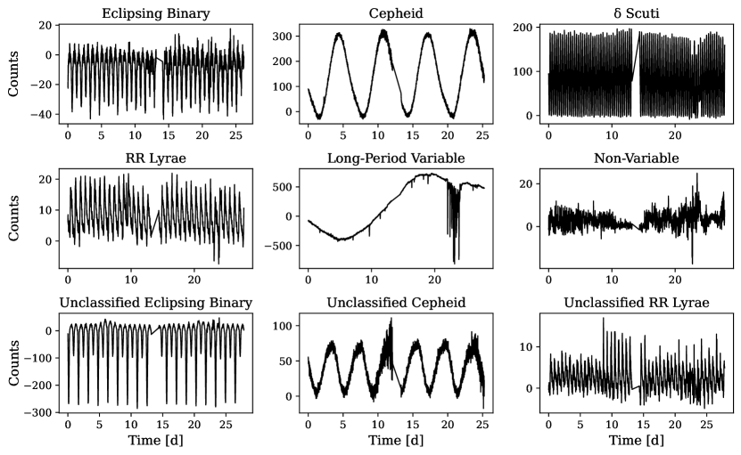
Figure 7: The light curves of eight variable stars characterized by the SourceDetect RFC. The top and middle rows contain previously discovered variable stars with classes matching the classifications made by the SourceDetect RFC. The bottom row has previously unclassified objects with variable classifications made by SourceDetect.

4.3 Minor Planets

TESS has an established history of bright $m_{r}<20$ minor planet detection and population analysis (Pál et al., 2018, 2020; Woods et al., 2021; McNeill et al., 2023). The high-cadence light curves enable shape fitting for asteroids (e.g. Humes & Hanuš, 2024) and characterization of comets (e.g. Ridden-Harper et al., 2021a). TESSELLATE provides asteroid detections as part of its transient pipeline; an example is shown in Figure 1 (lower center).

As TESSELLATE has a shallow magnitude limit of $\sim$17, only known minor planets will be recoverable. We identify all minor planets in a cut through SkyBoT queries (Berthier et al., 2006) and build ephemerides for all targets brighter than $m_{T}=18$ using information from the Minor Planet Center. Asteroid positions are cross referenced against TESSELLATE detections, which are then removed from the transient sample.

Although TESSELLATE only provides discrete detections of minor planets, we can perform forced photometry to extract lightcurves of all known objects. We stitch together lightcurves of asteroids that cross multiple cuts. The resulting high-cadence lightcurves of minor planets can be used to analyze object morphology and rotation/tumble periods. An example lightcurve segment for the asteroid (5254) Ulysses from Sector 29 is shown in Figure 8. With the Sector 29 light curve we identify a rotation period of $28.71\pm 0.01\;$hours, which is consistent with the asteroid Lightcurve Database (LCDB 2023 release, Warner et al., 2009). Population and individual target analysis with TESSELLATE will be released in upcoming work.

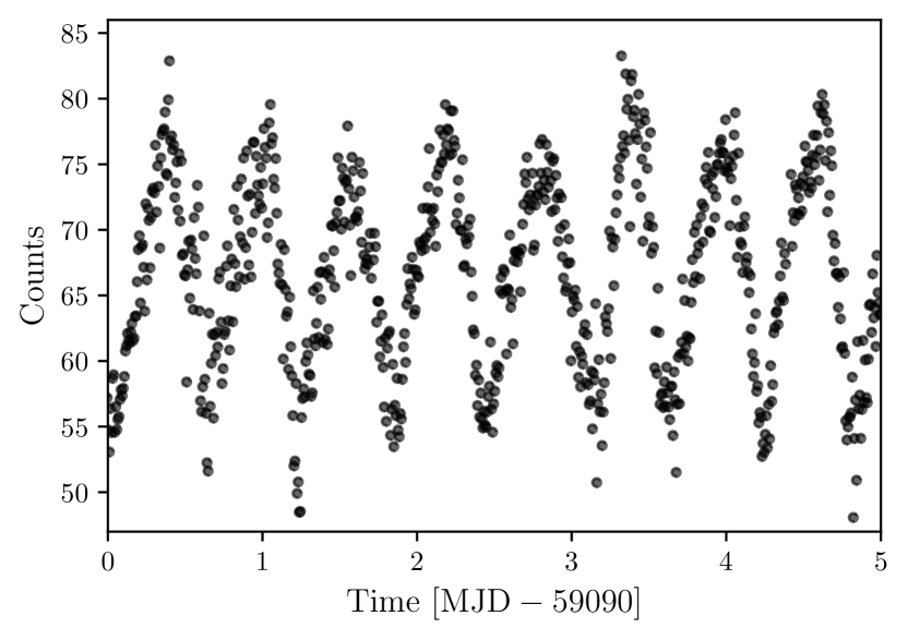
Figure 8: A section of the 10 minute cadence light curve of asteroid (5254) Ulysses from sector 29.

4.4 Flare Stars

Stellar flares are among the most common “transient” phenomena, and are the most numerous events in our sample. While they are contaminants for our fast extragalactic transient search, flare stars are valuable for understanding stellar processes, and atmospheric retention on exoplanets (Kowalski, 2024).

The complex nature of stellar flares produces a variety of different light curve profiles. While simple isolated flares appear as simple exponential declines, multiple flares can stack producing complex structures. For example, the flare star presented in Figure 1 exhibits first a simple and then a complex flare.

As flares evolve over minute timescales, high-cadence observations are required to study flare properties. While flares can be described with simple analytical models, only the 200 second cadence FFIs are fast enough to accurately recover flare parameters (Howard & MacGregor, 2021; Mendoza et al., 2022).

With TESSELLATE we can construct an all-sky catalog for flare stars. Once we process the 200 second data, we can also perform population statistics on flare properties.

4.5 Transiting Exoplanets

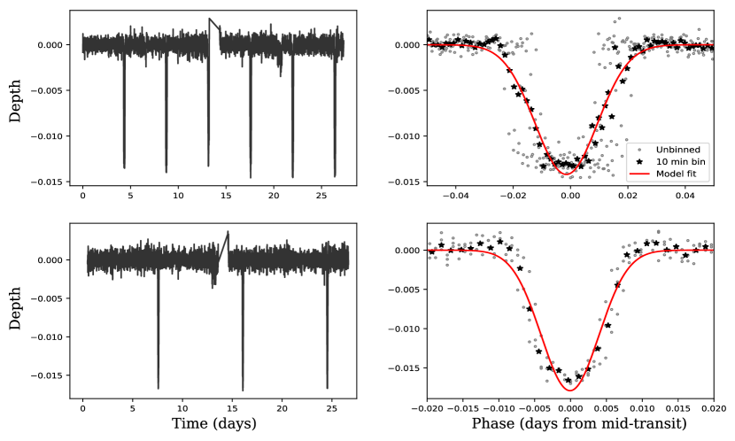
Figure 9: The light curves of known exoplanet host star WASP-62 (Top Panels) and a previously undiscovered exoplanet candidate (Bottom Panels). The left panels are replotted in their respective right panels after being phase-folded and fit with a standard Gaussian model (red line). Both of these objects were detected by SourceDetect.

Through our untargeted search, we are also able to detect transiting exoplanets. The post-processing pipeline that we discuss in § 2.8 has recovered known transiting exoplanets and produced tens of new candidates just from Sector 29 data. While other pipelines have conducted exoplanet searches of FFI data, they often impose magnitude limits. For example, the search described in Barclay et al. (2018) only considers stars with $I$ magnitudes $\leq 11$ for sun-like stars and $\leq 15$ for M-dwarfs. With TESSELLATE we impost no magnitude limit, and therefore are able to explore a new parameter space for identifying exoplanet candidates of faint stars.

For Cameras 3 and 4 in Sector 29, we recover 8 out of 27 known exoplanet host stars. Due to our search method, all known exoplanet candidates that we recover must have significant dips, therefore, we are unlikely to recover candidates with high contrast between stellar and planetary radii. In Figure 9 we show example light curves of the recovered exoplanet WASP-62 and a TESSELLATE exoplanet candidate.

As many of the host stars for TESSELLATE exoplanet candidates are faint, follow-up and confirmation will be challenging. As with transient detections, we will make all exoplanet candidates public as part of the TESS community target of interest program.

5 The TESSELLATE Sky Survey

TESS has observed $>90$% of the sky during its six years of operation, with most areas receiving multiple visits. With TESSELLATE, we can build an extensive catalog of variable sources that cover a broad range of astronomy. Following the vetting process outlined in § 2.7, we collate all targets and build the TESSELLATE Sky Survey (TSS).

The catalog will report all detected transient objects, including: flare stars, variable stars, exoplanet candidates, and all other transient phenomena. Minor planet detections will not be included in the catalog. These components each pass through their own vetting and classification processes: variable stars through the SourceDetect RFC, transient candidates through Zooniverse vetting, and negative-flux detections through the exoplanet pipeline.

The TSS catalog will be publicly available to support open science. Sources within the catalog are named with a convention that is dependent on their spatial and temporal coordinates. The base format we adopt for events is TSS JHHmm$\pm$DDddTttttt where TSS is the survey designation, HHmm is the hours & minutes components of the R.A., DDdd is the degrees and arcminutes component of the declination, and ttttt is the rounded MJD of the event. Sources that have numerous events per sector, such as active flare stars and variable stars, will follow a modified naming structure where the time component is dropped. Examples of this naming convention can be seen for the example light curves in Figure 1.

Once events are named, we build catalog profiles by cross referencing with existing source and transient catalogs. As the positional error for TESSELLATE events is $\sim$10^′′, multiple sources can be present inside the error region, complicating host identification. In such cases, we identify the most likely host though considering host position and color, which is then weighted by the morphology of the event light curve.

TSS data is processed per sector; we are starting with the 10 minute cadence data from Extended Mission 1, spanning sectors 27 to 55. This data finds a middle-ground between temporal resolution and data processing time. We will present the first catalog once data from the southern hemispheres has been processed.

6 Conclusion

We present TESSELLATE, the first pipeline capable of differencing and extracting transient events from all data stored in TESS FFIs. Using the TESSreduce difference imaging pipeline and a range of source detection techniques, the pipeline identifies variable sources in every frame across the entire detector. Since TESSELLATE is an untargeted search, there are no requirements placed on event or source type. It thus has the ability to discover new transient classes, new variable stars, and even new exoplanet candidates. These sources are compiled into a table of event candidates, which is subject to various quality cuts to produce a sample of variable and transient events.

Our pipeline is currently capable of detecting and distinguishing between variable stars, exoplanet candidates, and transients. These three main event classes are processed with specific vetting and characterization pipelines. Variable stars are classified by applying a random forest classifier to the light curves with the SourceDetect package. Exoplanet candidates are classified where possible with TRICERATOPS, however, many of our exoplanet candidates have faint host stars with insufficient data to reach a classification. Due to the complex and uncertain nature of fast transient lightcurves all TESSELLATE candidates are vetted by citizen scientists with the Cosmic Cataclysms project hosted by Zooniverse. Already we have thousands of transients classified through Cosmic Cataclysms, with which we are building a large labeled set of TESSlight curves which will be used to train a generalized fast transient classifier.

Events that pass our vetting criteria are included in the TESSELLATE sky survey catalog, which will contain information on likely hosts identified from deep imagining source catalogs with high spatial resolution. The catalog and pipeline light curves will be made open access for each of the two-year TESS missions; the first data release will be produced using the 10 minute cadence data from Extended Mission 1 covering sectors 27–55. Alongside supporting a multitude of science cases, this catalog could be cross-referenced by other surveys to readily remove repeating galactic transients such as flare stars.

The large search volume covered by TESS at high cadence allows us to search for unique rapid transients. Of the known fast transients we find it is unlikely that a kilonova will be observed by TESS, however, we expect a high number of FELTs, FBOTs and GRB afterglows to be present in the data. Since we do not impose any restrictions on the light curves of transient events, we will also search for new classes of fast transients. Alongside building a library of high cadence light curves for these events, we will be able to place strong constraints on their occurrence rates.

TESS observations now tile the sky multiple times, enabling an exploration of the rapid time domain. With TESSELLATE, we are able to piece together the variable sky and better understand our dynamic Universe.

References

- Abbott et al. (2017) Abbott, B. P., Abbott, R., Abbott, T., Acernese, F., et al. 2017, Physical review letters, 119, 161101
- Astropy Collaboration et al. (2013) Astropy Collaboration, Robitaille, T. P., Tollerud, E. J., et al. 2013, Astronomy and Astrophysics, 558, A33, doi: 10.1051/0004-6361/201322068
- Astropy Collaboration et al. (2018) Astropy Collaboration, Price-Whelan, A. M., Sipőcz, B. M., et al. 2018, AJ, 156, 123, doi: 10.3847/1538-3881/AABC4F
- Astropy Collaboration et al. (2022) Astropy Collaboration, Price-Whelan, A. M., Lim, P. L., et al. 2022, ApJ, 935, 167, doi: 10.3847/1538-4357/AC7C74
- Audenaert (2021) Audenaert, J. 2021, The Astronomical Journal, 162, doi: https://doi.org/10.3847/1538-3881/ac166a
- Barclay et al. (2018) Barclay, T., Pepper, J., & Quintana, E. V. 2018, The Astrophysical Journal Supplement Series, 239, 2, doi: 10.3847/1538-4365/aae3e9
- Barclay et al. (2012) Barclay, T., Still, M., Jenkins, J. M., Howell, S. B., & Roettenbacher, R. M. 2012, Monthly Notices of the Royal Astronomical Society, 422, 1219, doi: 10.1111/j.1365-2966.2012.20700.x
- Baron (2019) Baron, D. 2019, Machine Learning in Astronomy: a practical overview. https://arxiv.org/abs/1904.07248
- Bell & Higgins (2022) Bell, K. J., & Higgins, M. E. 2022, TESS_PRF: Display the TESS pixel response function, Astrophysics Source Code Library, record ascl:2207.008
- Bellm et al. (2019) Bellm, E. C., Kulkarni, S. R., Graham, M. J., et al. 2019, Publications of the Astronomical Society of the Pacific, 131, 018002, doi: 10.1088/1538-3873/aaecbe
- Benigo (2009) Benigo, Y. 2009, Foundations and Trends® in Machine Learning, 2, 1, doi: http://dx.doi.org/10.1561/2200000006
- Berthier et al. (2006) Berthier, J., Vachier, F., Thuillot, W., et al. 2006, ASPC, 351, 367. https://ui.adsabs.harvard.edu/abs/2006ASPC..351..367B/abstract
- Boyle et al. (2024) Boyle, R. S., Littlefield, C., Garnavich, P., et al. 2024, AJ, 167, 71, doi: 10.3847/1538-3881/acf718
- Bradley et al. (2024) Bradley, L., Sipőcz, B., Robitaille, T., et al. 2024, astropy/photutils: 1.13.0, Zenodo, doi: 10.5281/zenodo.12585239
- Brasseur et al. (2019) Brasseur, C. E., Phillip, C., Fleming, S. W., Thompson, S. E., & White, R. L. 2019, Astrophysics Source Code Library
- Bruch (2022) Bruch, A. 2022, Monthly Notices of the Royal Astronomical Society, 514, 4718, doi: 10.1093/mnras/stac1650
- Caldwell et al. (2020) Caldwell, D. A., Tenenbaum, P., Twicken, J. D., et al. 2020, Research Notes of the American Astronomical Society, 4, 201, doi: 10.3847/2515-5172/abc9b3
- Chambers et al. (2016) Chambers, K. C., Magnier, E. A., Metcalfe, N., et al. 2016. https://arxiv.org/abs/1612.05560v4
- Dobrycheva et al. (2023) Dobrycheva, D. V., Vasylenko, M. Y., Kulyk, I. V., et al. 2023, Kosmichna Nauka i Tekhnologiya, 29, 68, doi: 10.15407/knit2023.06.068
- Drlica-Wagner et al. (2021) Drlica-Wagner, A., Carlin, J. L., Nidever, D. L., et al. 2021, ApJS, 256, 2, doi: 10.3847/1538-4365/ac079d
- Drout et al. (2014) Drout, M. R., Chornock, R., Soderberg, A. M., et al. 2014, The Astrophysical Journal, 794, 23
- Elizabethson (2023) Elizabethson, A. 2023, The Astronomical Journal, 166, doi: https://doi.org/10.3847/1538-3881/acf865
- Eyer et al. (2023) Eyer, L., Audard, M., Holl, B., et al. 2023, A&A, 674, A13, doi: 10.1051/0004-6361/202244242
- Farnham et al. (2021) Farnham, T. L., Kelley, M. S. P., & Bauer, J. M. 2021, \psj, 2, 236, doi: 10.3847/PSJ/ac323d
- Fausnaugh et al. (2021) Fausnaugh, M. M., Vallely, P. J., Kochanek, C. S., et al. 2021, The Astrophysical Journal, 908, 51, doi: 10.3847/1538-4357/abcd42
- Fausnaugh et al. (2023) Fausnaugh, M. M., Vallely, P. J., Tucker, M. A., et al. 2023, The Astrophysical Journal, 956, 108, doi: 10.3847/1538-4357/aceaef
- Fausnaugh et al. (2023) Fausnaugh, M. M., Jayaraman, R., Vanderspek, R., et al. 2023, Research Notes of the American Astronomical Society, 7, 56, doi: 10.3847/2515-5172/acc4c5
- Feinstein et al. (2020) Feinstein, A. D., Montet, B. T., Ansdell, M., et al. 2020, AJ, 160, 219, doi: 10.3847/1538-3881/abac0a
- Fetherolf et al. (2023) Fetherolf, T., Pepper, J., Simpson, E., et al. 2023, The Astrophysical Journal Supplement Series, 268, 4, doi: 10.3847/1538-4365/acdee5
- Freeburn et al. (2024) Freeburn, J., Cooke, J., Möller, A., et al. 2024, MNRAS, 531, 4836, doi: 10.1093/mnras/stae1489
- Fulton et al. (2020) Fulton, M., Smith, K. W., Wright, D. E., et al. 2020, Transient Name Server AstroNote, 255, 1
- Garrison et al. (2024) Garrison, L. H., Foreman-Mackey, D., hsuan Shih, Y., & Barnett, A. 2024, Research Notes of the AAS, 8, 250, doi: 10.3847/2515-5172/ad82cd
- Ghirlanda et al. (2013) Ghirlanda, G., Ghisellini, G., Salvaterra, R., et al. 2013, MNRAS, 428, 1410, doi: 10.1093/mnras/sts128
- Giacalone & Dressing (2020) Giacalone, S., & Dressing, C. D. 2020, triceratops: Candidate exoplanet rating tool. http://ascl.net/2002.004
- Giacalone et al. (2021) Giacalone, S., Dressing, C. D., Jensen, E. L. N., et al. 2021, The Astronomical Journal, 161, 24, doi: 10.3847/1538-3881/abc6af
- Ginsburg et al. (2019) Ginsburg, A., Sipőcz, B. M., Brasseur, C. E., et al. 2019, AJ, 157, 98, doi: 10.3847/1538-3881/aafc33
- Günther et al. (2020) Günther, M. N., Zhan, Z., Seager, S., et al. 2020, The Astronomical Journal, 159, 60, doi: 10.3847/1538-3881/ab5d3a
- Harris et al. (2020) Harris, C. R., Millman, K. J., van der Walt, S. J., et al. 2020, Nature, 585, 357, doi: 10.1038/s41586-020-2649-2
- Heinze et al. (2018) Heinze, A. N., Tonry, J. L., Denneau, L., et al. 2018, AJ, 156, 241, doi: 10.3847/1538-3881/aae47f
- Hinton & Salakhutdinov (2006) Hinton, G. E., & Salakhutdinov, R. R. 2006, Science, 313, 504, doi: 10.1126/science.1127647
- Ho et al. (2023) Ho, A. Y., Perley, D. A., Gal-Yam, A., et al. 2023, The Astrophysical Journal, 949, 120
- Howard & MacGregor (2021) Howard, W. S., & MacGregor, M. A. 2021, ApJ, 926, 204, doi: 10.3847/1538-4357/ac426e
- Humes & Hanuš (2024) Humes, O. A., & Hanuš, J. 2024, arXiv, arXiv:2412.04123, doi: 10.48550/ARXIV.2412.04123
- Hunter (2007) Hunter, J. D. 2007, Computing in Science and Engineering, 9, 90, doi: 10.1109/MCSE.2007.55
- Jayaraman et al. (2024) Jayaraman, R., Fausnaugh, M., Ricker, G. R., Vanderspek, R., & Mo, G. 2024, The Astrophysical Journal, 972, 162, doi: 10.3847/1538-4357/ad5e7b
- Jayasinghe et al. (2018) Jayasinghe, T., Kochanek, C. S., Stanek, K. Z., et al. 2018, MNRAS, 477, 3145, doi: 10.1093/mnras/sty838
- Kato & Osaki (2013a) Kato, T., & Osaki, Y. 2013a, Publications of the Astronomical Society of Japan, 65, L13, doi: 10.1093/pasj/65.6.L13
- Kato & Osaki (2013b) —. 2013b, Publications of the Astronomical Society of Japan, 65, 97, doi: 10.1093/pasj/65.5.97
- Kowalski (2024) Kowalski, A. F. 2024, LRSP, 21, 1, doi: 10.1007/S41116-024-00039-4
- Kunimoto et al. (2024) Kunimoto, M., DeRocco, W., Smyth, N., & Bryson, S. 2024. http://arxiv.org/abs/2404.11666
- LeCun et al. (2015) LeCun, Y., Benigo, & Hinton, G. 2015, Nature, 521, 436, doi: https://doi.org/10.1038/nature14539
- Liu & Qian (2023) Liu, W., & Qian, S. 2023, The Astrophysical Journal, 954, 135, doi: 10.3847/1538-4357/acebdf
- McKinney (2010) McKinney, W. 2010, in Proceedings of the 9th Python in Science Conference, ed. Stéfan van der Walt & Jarrod Millman, 56 – 61, doi: 10.25080/Majora-92bf1922-00a
- McNeill et al. (2023) McNeill, A., Gowanlock, M., Mommert, M., et al. 2023, The Astronomical Journal, 166, 152, doi: 10.3847/1538-3881/ACF194
- Mendoza et al. (2022) Mendoza, G. T., Davenport, J. R. A., Agol, E., Jackman, J. A. G., & Hawley, S. L. 2022, The Astronomical Journal, 164, 17, doi: 10.3847/1538-3881/ac6fe6
- Metzger (2020) Metzger, B. D. 2020, Kilonovae, Springer, doi: 10.1007/s41114-019-0024-0
- Mo et al. (2023) Mo, G., Jayaraman, R., Fausnaugh, M., et al. 2023, ApJ, 948, L3, doi: 10.3847/2041-8213/acca70
- Moore et al. (in prep.) Moore, A., Ridden-Harper, R., et, & al. in prep.
- Mróz (2024) Mróz, P. 2024, Acta Astron., 73, 259, doi: 10.32023/0001-5237/73.4.1
- Pala et al. (2020) Pala, A. F., Gänsicke, B. T., Breedt, E., et al. 2020, MNRAS, 494, 3799, doi: 10.1093/mnras/staa764
- pandas development team (2020) pandas development team, T. 2020, pandas-dev/pandas: Pandas, latest, Zenodo, doi: 10.5281/zenodo.3509134
- Pedregosa et al. (2011) Pedregosa, F., Varoquaux, G., Gramfort, A., et al. 2011, Journal of Machine Learning Research, 12, 2825
- Perley et al. (2025) Perley, D. A., Ho, A. Y. Q., Fausnaugh, M., et al. 2025, Monthly Notices of the Royal Astronomical Society, staf125, doi: 10.1093/mnras/staf125
- Pietras et al. (2022) Pietras, M., Falewicz, R., Siarkowski, M., Bicz, K., & Preś, P. 2022, The Astrophysical Journal, 935, 143, doi: 10.3847/1538-4357/ac8352
- Pál et al. (2018) Pál, A., Molnár, L., & Kiss, C. 2018, Publications of the Astronomical Society of the Pacific, 130, 114503, doi: 10.1088/1538-3873/aae2aa
- Pál et al. (2020) Pál, A., Szakáts, R., Kiss, C., et al. 2020, The Astrophysical Journal Supplement Series, 247, 26, doi: 10.3847/1538-4365/ab64f0
- Ricker et al. (2014) Ricker, G. R., Winn, J. N., Vanderspek, R., et al. 2014, Journal of Astronomical Telescopes, Instruments, and Systems, 1, 014003, doi: 10.1117/1.jatis.1.1.014003
- Ridden-Harper et al. (2021a) Ridden-Harper, R., Bannister, M. T., & Kokotanekova, R. 2021a, Research Notes of the American Astronomical Society, 5, 161, doi: 10.3847/2515-5172/ac1512
- Ridden-Harper et al. (2021b) Ridden-Harper, R., Rest, A., Hounsell, R., et al. 2021b, arXiv e-prints, arXiv:2111.15006. https://arxiv.org/abs/2111.15006
- Ridden-Harper et al. (2020) Ridden-Harper, R., Tucker, B. E., Gully-Santiago, M., et al. 2020, Monthly Notices of the Royal Astronomical Society, 498, 33–43, doi: 10.1093/mnras/staa2247
- Ridden-Harper et al. (2019) Ridden-Harper, R., Tucker, B. E., Garnavich, P., et al. 2019, MNRAS, 490, 5551, doi: 10.1093/mnras/stz2923
- Roxburgh et al. (2023) Roxburgh, H., Ridden-Harper, R., Lane, Z. G., et al. 2023, arXiv e-prints, arXiv:2307.11294, doi: 10.48550/arXiv.2307.11294
- Ryan et al. (2020) Ryan, G., van Eerten, H., Piro, L., & Troja, E. 2020, ApJ, 896, 166, doi: 10.3847/1538-4357/ab93cf
- Smith et al. (2021) Smith, K. L., Ridden-Harper, R., Fausnaugh, M., et al. 2021, The Astrophysical Journal, 911, 43, doi: 10.3847/1538-4357/abe6a2
- Stringer et al. (2019) Stringer, K. M., Long, J. P., Macri, L. M., et al. 2019, AJ, 158, 16, doi: 10.3847/1538-3881/ab1f46
- Tonry (2011) Tonry, J. L. 2011, Publications of the Astronomical Society of the Pacific, 123, 58, doi: 10.1086/657997
- Troja (2023) Troja, E. 2023, doi: 10.3390/universe9060245
- Udalski et al. (2015) Udalski, A., Szymański, M. K., & Szymański, G. 2015, AcA, 65, 1, doi: 10.48550/ARXIV.1504.05966
- Udalski et al. (1992) Udalski, A., Szymanski, M., Kaluzny, J., et al. 1992, AcA, 42, 253. https://ui.adsabs.harvard.edu/abs/1992AcA....42..253U/abstract
- Vallely et al. (2021) Vallely, P. J., Kochanek, C. S., Stanek, K. Z., Fausnaugh, M., & Shappee, B. J. 2021, Monthly Notices of the Royal Astronomical Society, 500, 5639, doi: 10.1093/mnras/staa3675
- Vanderspek et al. (2018) Vanderspek, R., Doty, J., Fausnaugh, M., et al. 2018, TESS Instrument Handbook, Tech. rep., Kavli Institute for Astrophysics and Space Science, Massachusetts Institute of Technology.
- Villar et al. (2017) Villar, V. A., Guillochon, J., Berger, E., et al. 2017, The Astrophysical Journal Letters, 851, L21
- Virtanen et al. (2020) Virtanen, P., Gommers, R., Oliphant, T. E., et al. 2020, Nature Methods 2020 17:3, 17, 261, doi: 10.1038/s41592-019-0686-2
- Wang et al. (2023) Wang, Q., Armstrong, P., Zenati, Y., et al. 2023, ApJ, 943, L15, doi: 10.3847/2041-8213/acb0d0
- Wang et al. (2024) Wang, Q., Rest, A., Dimitriadis, G., et al. 2024, ApJ, 962, 17, doi: 10.3847/1538-4357/ad0edb
- Warner (1986) Warner, B. 1986, MNRAS, 222, 11, doi: 10.1093/mnras/222.1.11
- Warner et al. (2009) Warner, B. D., Harris, A. W., & Pravec, P. 2009, Icar, 202, 134, doi: 10.1016/J.ICARUS.2009.02.003
- Wei & Shengbang (2023) Wei, L., & Shengbang, Q. 2023, ApJ, 954, 135, doi: 10.3847/1538-4357/acebdf
- Woods et al. (2021) Woods, D. F., Ruprecht, J. D., Kotson, M. C., et al. 2021, PASP, 133, 014503, doi: 10.1088/1538-3873/ABC761
- Yang et al. (2024) Yang, H., Weicheng, Z., Tianjun, G., et al. 2024, The Astrophysical Journal Letters, 972, L12, doi: 10.3847/2041-8213/ad6c3c
- Zieba et al. (2019) Zieba, S., Zwintz, K., Kenworthy, M. A., & Kennedy, G. M. 2019, A&A, 625, L13, doi: 10.1051/0004-6361/201935552