Well-posedness of the initial boundary value problem
for the motion of an inextensible hanging string
Tatsuo Iguchi and Masahiro Takayama***Corresponding author
Abstract
We consider the motion of an inextensible hanging string of finite length under the action of the gravity. The motion is governed by nonlinear and nonlocal hyperbolic equations, which is degenerate at the free end of the string. We show that the initial boundary value problem to the equations of motion is well-posed locally in time in weighted Sobolev spaces at the quasilinear regularity threshold under a stability condition. This paper is a continuation of our preceding articles [1, 2].
1 Introduction
We consider the initial boundary value problem to the motion of an inextensible hanging string of finite length under the action of the gravity, where one end of the string is fixed and another one is free. We also consider the problem in the case without any external forces. After an appropriate scaling, the equations of motion have the form
| (1.1) |
under the boundary conditions
| (1.2) |
where is the position vector of the string at time with the arc length parametrization measured from the free end of the string, is the tension of the string, and is the acceleration of gravity vector, which is assumed to be a constant unit vector or the zero vector; see Figure 1.1.
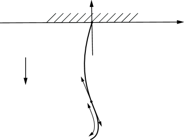
Here, and denote the derivatives of with respect to and , respectively. For details on these equations, we refer to Reeken [7], Yong [10], and Iguchi and Takayama [1]. We consider the initial boundary value problem of the above equations under the initial conditions
| (1.3) |
Our objective in this paper is to establish the well-posedness locally in time of the initial boundary value problem (1.1)–(1.3) under the stability condition
| (1.4) |
for in the class with , where is a weighted Sobolev space of order on the interval ; see Section 2 for the definition of the space . Here, we note that in this problem is an unknown quantity as well as . As is well-known, once and are given, is uniquely determined as a unique solution of the two-point boundary value problem
| (1.5) |
Therefore, can be regarded as a function of and , so that the first equation in (1.1) can be regarded as nonlinear wave equations for , which are degenerate at the free end where . However, this dependence is nonlocal in space and causes a nonlocal character of the equations.
Our main result in this paper is given by the following theorem.
Theorem 1.1.
For any integer and any positive constants and , there exists a small positive time such that if the initial data satisfy
| (1.6) |
where is the initial tension, and the compatibility conditions up to order in the sense of Definition 3.2, then the initial boundary value problem (1.1)–(1.3) has a unique solution satisfying and the stability condition (1.4). Moreover, we have in the case and for any in the case .
Remark 1.2.
-
(1)
The initial tension is uniquely determined from the initial data as a unique solution of the two-point boundary value problem (1.5) in the case . Moreover, as was shown in Iguchi and Takayama [1, Lemma 3.4], we have
if the right-hand side is non-negative. Therefore, if the string is in fact hanging initially, that is to say, if , then the stability condition is initially satisfied.
-
(2)
In the case , that is, in the case without any external forces, if , then the initial boundary value problem (1.1)–(1.3) has a unique global solution , which does not satisfy the stability condition (1.4); see [1, Theorem 2.4]. On the other hand, if , then the stability condition is initially and automatically satisfied.
- (3)
-
(4)
As was explained in [1, Remark 2.2], the requirement corresponds to the quasilinear regularity in the sense that is the minimal integer regularity index that ensures the embedding . Therefore, is a critical regularity index in the classical sense.
- (5)
As was shown in [1, Theorem 2.5], in the class of solutions stated in Theorem 1.1 the initial boundary value problem (1.1)–(1.3) is equivalent to
| (1.7) |
| (1.8) |
| (1.9) |
under the restrictions and on the initial data and the stability condition (1.4). In other words, we can remove the constraint from the equations. Therefore, it is sufficient to show the well-posedness of this transformed problem (1.7)–(1.9).
Well-posedness of a linearized problem to the nonlinear one (1.7)–(1.9) was established by Iguchi and Takayama [2] in the class of the weighted Sobolev space. However, the map reveals a loss of twice derivatives, where denote variations in the linearization to the nonlinear problem around , so that the standard Picard iteration cannot be applicable directly to show the existence of solution to the nonlinear problem. To overcome this difficulty, we implement a quasilinearization procedure and reduce the nonlinear problem into a quasilinear one equivalently introducing new unknowns by
| (1.10) |
Then, we can solve the quasilinear problem for unknowns by applying the existence theory established in [2] and by a standard fixed point argument. This procedure works well under the additional regularity assumption .
To show the well-posedness in the case , we approximate the initial data by regular ones, which must satisfy higher order compatibility conditions, and construct a sequence of solutions for the approximate initial data. Thanks to the a priori estimate of the solution obtained in Iguchi and Takayama [1], we obtain a uniform bound of the solutions. Then, by the standard compactness argument, we can extract a subsequence of solutions which converges the desired solution. However, we face a difficulty in the approximation process of the initial data due to the nonlocal character of the problem, so that we need to study the compatibility conditions in detail.
It is well-known that in the theory of the initial boundary value problem for hyperbolic systems with an unknown , if the boundary is non-characteristic, then the initial data satisfying compatibility conditions up to order can be approximated by a sequence of more regular data with a positive integer , which converges to in and satisfy the compatibility conditions up to order , where is the standard Sobolev space of order . See, for example, Rauch and Massay [6]. To construct such approximate data, we first approximate the initial data by , which converges to in . Generally, does not satisfy the compatibility conditions. Therefore, we need to modify the data by adding an appropriate function so that converges to in and that satisfies the compatibility conditions. To this end, we usually use the following structure of the system: are determined from the initial data through the hyperbolic system and have the form
where is an invertible matrix. In this situation, by adding with an appropriate constant vector to the initial data we can modify for whatever we want keeping the values of unchanged for . For our problem (1.7)–(1.8), roughly speaking, have the form
where are functionals defined in appropriate weighted Sobolev spaces, so that is not linear with respect to due to these nonlocal terms . This nonlocal character is caused by the tension of the string. Moreover, if we add to the initial data to modify the value of , then all the values of for would change due to the nonlocal terms. Therefore, the standard technique for approximation of the initial data cannot be applicable directly to our problem.
Our strategy to overcome this difficulty is to approximate the initial data in the form
where is a smooth approximation of the initial data , is defined for by with a cut-off function satisfying for , and are small positive parameters; this function is naturally extended for as . Then, we can regard the compatibility conditions as equations for , which are nonlinear contrary to the standard initial boundary value problems for nonlinear hyperbolic systems. However, the nonlinearity becomes as weak as we want by choosing the parameters and sufficiently small. Therefore, we can apply the implicit function theorem to solve the equations for if is sufficiently close to in an appropriate norm. To carry out this strategy, we use the continuity of the map as well as the discontinuity of the map at . We also need to study the nonlocal terms in detail.
The contents of this paper are as follows. In Section 2, which is a preliminary section, we introduce weighted Sobolev spaces and for non-negative integer and present basic properties of these spaces and related calculus inequalities. We also present estimates of solutions to a two-point boundary value problem related to (1.8). In Section 3 we state precisely the compatibility conditions for the initial boundary value problem (1.1)–(1.3) and for the problem (1.7)–(1.9). Then, we state Propositions 3.3 and 3.4, which ensure that the initial data for the problem (1.1)–(1.3) and for the problem (1.7)–(1.9) can be approximated by smooth initial data satisfying higher order compatibility conditions. Since our proofs of these propositions are technical and long, we postpone them until Sections 6 and 7. In Section 4 we derive a quasilinear system of equations for unknowns , where and are defined by (1.10), and state Proposition 4.2 which ensures the well-posedness locally in time of the initial boundary value problem for the quasilinear system in the class and with . The proposition is proved by applying our previous result [2, Theorem 2.8] on the well-posedness of the initial boundary value problem to a linearized system for the nonlinear problem (1.1)–(1.3) and by a standard fixed point argument. In Section 5 we prove our main result in this paper, that is, Theorem 1.1. The proof is divided into three cases: the case , the case , and the critical case . The case is proved by showing that the solution for the quasilinear system obtained in Section 4 with appropriately prepared initial data is in fact a solution of the reduced nonlinear problem (1.7)–(1.9) and satisfies the desired regularity. In order to show the theorem in the case and , we first approximate the initial data by regular ones satisfying higher order compatibility conditions by using Proposition 3.4 and then construct corresponding approximate solutions by using the result in the first case. Thanks to the a priori estimate obtained in [1, Theorem 2.1] with a slight improvement and a standard compactness argument, we can show that the approximate solutions converge to the desired solution. A difficulty in showing the strong continuity in time of the solution appears in the critical case . To overcome this difficulty, we make use of the energy estimate. In Section 6 we give a proof of Proposition 3.3 on an approximation of the initial data for the problem (1.7)–(1.9). In Section 7 we give a proof of Proposition 3.4 on an approximation of the initial data for the problem (1.1)–(1.3) by modifying the calculations in Section 6 in order that the approximate initial data also satisfy the constraints and for . Finally, in Section 8 we give a remark on the improvement of the a priori estimate of the solution.
Notation. For , we denote by the Lebesgue space on the open interval . For non-negative integer , we denote by the Sobolev space of order on . The norm of a Banach space is denoted by . The inner product in is denoted by . We put and . The norm of a weighted space with a weight is denoted by , so that for . It is sometimes denoted by , too. This would cause no confusion. For a map defined in an open set in a Banach space and with a value in a Banach space , we denote by the Fréchet derivative of at . The application of the linear bounded operator to is denoted by . denotes the commutator. We denote by a positive constant depending on . means that there exists a non-essential positive constant such that holds. means that and hold. .
Acknowledgement
T. I. is partially supported by JSPS KAKENHI Grant Number JP23K22404.
2 Preliminaries
In this preliminary section, we recall the definition of the weighted Sobolev spaces and and present basic properties of these spaces and related calculus inequalities. They were proved in Takayama [9] and Iguchi and Takayama [1, 2].
2.1 Function spaces and known properties
For a non-negative integer , following Reeken [7, 8], Takayama [9], and Iguchi and Takayama [1], we define a weighted Sobolev space as a set of all function equipped with a norm defined by
Preston [5] used a weighted Sobolev space equipped with a norm defined by . Apparently the weights of these norms and are different, they are actually equivalent so that we have . We will use another weighted Sobolev space equipped with a norm , which is defined so that holds. For more details, we refer to [1].
For a function depending also on time and for integers and satisfying , we introduce norms and by and , respectively, and put , , and , . Corresponding to these norms, we define the spaces , , , and similarly, , , . We will solve the initial boundary value problem (1.1)–(1.3) in the class . However, in the critical case , we need to use a weaker norm than to evaluate . For , we introduce norms for as
and put and . As we will see in Lemma 2.14, for each the norm satisfies the equivalence
| (2.1) |
The weighted Sobolev space is characterize as follows: Let be the unit disc in and the Sobolev space of order on . For a function defined in the open interval , we define which is a function on .
Lemma 2.1 ([9, Proposition 3.2]).
Let be a non-negative integer. The map is bijective and it holds that for any .
Lemma 2.2 ([1, Lemma 4.5]).
For a non-negative integer , we have , , and .
Lemma 2.3 ([1, Lemma 4.7]).
It holds that for .
Lemma 2.4 ([1, Lemma 9.1]).
If , then we have
Lemma 2.5 ([2, Lemma 3.9]).
Let and be integers such that . If , then we have
Lemma 2.6 ([1, Lemma 4.10]).
It holds that
Lemma 2.7 ([2, Lemma 3.13]).
For a positive integer , we have
Lemma 2.8 ([1, Lemma 4.11]).
If , then we have
Lemma 2.9 ([2, Lemma 3.15]).
Let be a positive integer. If , then we have
Lemma 2.10 ([2, Lemma 3.16]).
If , then we have
2.2 Further properties of the weighted Sobolev spaces
By the definition of the norms and , we see easily the following lemma.
Lemma 2.11.
For a non-negative integer , it holds that and .
In view of Lemma 2.1 together with the standard tame estimates in the Sobolev space , we have the following tame estimates in the weighted Sobolev space .
Lemma 2.12.
It holds that for .
Lemma 2.13.
Let be a non-negative integer, an open set in , a compact set in , and . There exists a positive constant such that if takes its value in , then we have .
Lemma 2.14.
For each , the equivalence (2.1) holds.
Proof.
For , we see that
Therefore, putting with we have
Plugging in the above inequality, we obtain . Here, by integration by parts we see that
These estimates together with the Sobolev embedding imply . Conversely, by integration by parts we see that
which implies . Therefore, we obtain the equivalence (2.1) in the case . The other cases can be proved in the same way so we omit it. ∎
By Lemma 2.3, the weighted Sobolev space is an algebra if . A similar algebraic property of the weighted Sobolev space can follow from Lemma 2.6. To show this, we first prepare the following lemma.
Lemma 2.15.
For , we have . Particularly, for any non-negative integer , we have .
Proof.
Since and , by integration by parts, we see that
which yields . Particularly, we have . This together with the identity implies the equivalence . ∎
Lemma 2.16.
Let be a non-negative integer. Then, we have
Proof.
By Lemmas 2.8 and 2.15, we can also obtain the following lemma. Since the proof is almost the same as that of Lemma 2.16, we omit it.
Lemma 2.17.
Let be a non-negative integer. If , then, we have
We will use an averaging operator introduced in [1], which is defined by
| (2.2) |
Lemma 2.18 ([1, Corollary 4.13]).
Let be a non-negative integer, , and . Then, we have . Particularly, holds for .
Lemma 2.19.
Let be a non-negative integer and . If , then we have
2.3 Two-point boundary value problem
In view of (1.5) we consider the two-point boundary value problem
| (2.3) |
where and are given functions and is a constant.
Lemma 2.20 ([1, Lemmas 3.5 and 3.7]).
For any there exists a constant such that if , then the solution to the two-point boundary value problem (2.3) satisfies
for any and any satisfying .
Lemma 2.21.
For any and any integer there exists a constant such that if , then the solution to the two-point boundary value problem (2.3) with satisfies
3 Compatibility conditions
Let be a smooth solution of the problem (1.7)–(1.9) and put and for . These initial values are determined, at least formally, from the initial data as follows. As was explained in Remark 1.2 (1), the initial tension is determined as a unique solution of the two-point boundary value problem (1.8) in the case . Then, putting in the first equation in (1.7) we have . Now, suppose that and with an integer . Differentiating (1.8) -times with respect to and then putting , we obtain
| (3.1) |
where has been already determined as
By solving this two-point boundary value problem, is uniquely determined. Then, differentiating the first equation in (1.7) -times with respect to and then putting , we obtain
| (3.2) |
so that is determined. This procedure can be continued up to a certain order depending on the regularity of the initial data . More precisely, we have the following lemma.
Lemma 3.1.
Proof.
The case is trivial. The case was proved in [1, Sections 8 and 9]. Therefore, it is sufficient to show the case . It follows from Lemma 2.20 together with and that
so that we have . By Lemmas 2.6 and 2.8, we see that
so that we have . By Lemma 2.4, we have
Moreover, for any we see also that
where we used which was shown in [1, Lemma 4.3] and also follows from a sharper estimate given in the proof of Lemma 2.14. These estimates imply . ∎
Differentiating the first boundary condition in (1.7) -times with respect to and then putting , we obtain
| (3.3) |
This is a compatibility condition at order for the problem (1.7)–(1.9). Under the assumptions in Lemma 3.1, the lemma and the Sobolev embedding theorem imply for , so that the traces are defined. Therefore, the compatibility conditions make sense for .
Definition 3.2.
The following propositions ensure that the initial data for the problem (1.7)–(1.9) and for the problem (1.1)–(1.3) can be approximated by smooth initial data satisfying higher order compatibility conditions. These propositions are a key to show our main result Theorem 1.1 in the case .
Proposition 3.3.
Proposition 3.4.
If, in addition to the assumptions of Proposition 3.3, and the initial data satisfies and for , then the approximated initial data can be constructed such that and holds for .
4 Quasilinear problem
As was shown in Iguchi and Takayama [2], a linearized problem for unknowns to the nonlinear problem (1.1)–(1.3) around can be solved uniquely in a weighted Sobolev space. However, the map reveals loss of twice derivatives. A standard procedure to overcome this difficulty is to reduce the nonlinear problem into a quasilinear problem introducing new quantities.
4.1 Derivation of the quasilinear problem
For our problem, it is convenient to introduce new unknowns by
| (4.1) |
Differentiating (1.1), (1.2), and (1.5) twice with respect to , we obtain
| (4.2) |
and
| (4.3) |
where
| (4.4) |
These equations are used to determine . On the other hand, to determine we use (4.1), that is,
| (4.5) |
In this section, we will show the well-posedness of the initial boundary value problem (4.2)–(4.5) for unknowns in a weighted Sobolev space.
4.2 Compatibility conditions for the quasilinear problem
Before going to show the well-posedness, we explain compatibility conditions for this problem. Let be a smooth solution of (4.2)–(4.5) and put for . These initial values are determined, at least formally, from the initial data . In fact, these initial values are determined inductively as follows: Suppose that and are determined for a non-negative integer . It follows from (4.5) that and so that and are determined. Differentiating (4.3) -times with respect to and then putting , we see that
where is a polynomial of , , and their derivatives, so that is already determined. This two-point boundary value problem for is uniquely solved so that and are determined. Differentiating (4.2) -times with respect to and then putting , we see that is a polynomial , , and their derivatives, so that is also determined. On the other hand, differentiating the boundary condition in (4.2) -times with respect to and then putting we have
| (4.6) |
This is the compatibility condition at order for the problem (4.2)–(4.5). As will be shown in Lemma 4.1, if and with , then is in fact determined as a function in for . Therefore, the compatibility conditions make sense up to order .
Lemma 4.1.
For any integer and any positive constants , there exists a positive constant such that if the initial data satisfy
| (4.7) |
then the initial values defined above satisfy .
Proof.
This lemma can be proved by a similar argument to that in [1, Sections 8 and 9]. Here, for completeness we give a proof. For simplicity, we omit the superscript “in” from the notation so that we write , and instead of , and , respectively, throughout the proof. For an integer , we put
Then, it is sufficient to show that . Since and , it is not difficult to see that holds for . Therefore, by Lemma 2.4 we see that
so that
| (4.8) |
for . On the other hand, for we have
where . Therefore, by Lemma 2.21 together with and , we obtain
for . To evaluate , note first that by Lemmas 2.6 and 2.8 we have
for , if . Therefore, we see that
so that . Particularly, we obtain
| (4.9) |
for . Now, using (4.8) and (4.9) inductively we obtain . In fact, by the assumptions of the lemma we have . Suppose that holds for some . Then, it follows from (4.9) that and then from (4.8) that . Therefore, by induction we obtain the desired estimates. ∎
4.3 Well-posedness of the quasilinear problem
Proposition 4.2.
For any integer and any positive constants and , there exists a small positive time such that if the initial data satisfy (4.7), the stability condition
| (4.10) |
and the compatibility conditions (4.6) up to order , then the initial boundary value problem (4.2)–(4.5) has a unique solution on the time interval satisfying , , and the stability condition (1.4).
Proof.
By Lemma 4.1, we can determine the initial values for and for , which satisfy for and for . For , we define the set of all satisfying
| (4.11) |
In view of Lemma 2.1, it is standard to check that there exist a small and large such that .
For given , we consider the initial boundary value problem (4.2) and (4.3) for unknowns , where and are defind by (4.4). By Lemma 2.5, we have
As for , we decompose it as with and . By Lemma 2.9, we have . By Lemma 2.7, we have also in the case ; and and in the case . Moreover, in the case , by Lemma 2.2 we have . Furthermore, by Lemmas 2.7 and 2.9 we have . Therefore,
Particularly, we have , , , and . On the other hand, it is straightforward to see that the data satisfy the compatibility conditions up to order . Therefore, we can apply the existence theorem [2, Theorem 2.8], which guarantees the unique existence of a solution to the initial boundary value problem (4.2) and (4.3) in the class and . Moreover, the solution satisfies
| (4.12) | ||||
where we denote the constants and . These constants may change from line to line. We have also
| (4.13) | ||||
We define a map by .
By using this solution , we define as a unique solution to (4.5). Obviously, satisfy the conditions in the first two lines in (4.11). By (4.12) and (4.13), we have also
where we denote the constants and and used Lemma 4.1 to evaluate initial values. Now, we define the constants as , , , and choose the time so small that , , and . Then, we see that satisfy all the conditions in (4.11). We define a map by . We have shown that there exist large constants and a small time such that the set is not empty and that maps into itself. In the following we fix these constants.
We first take arbitrarily. Then, we define inductively
for . is a sequence of approximate solutions to the initial value problem for the quasilinear system (4.2)–(4.5). We note that satisfy the uniform bounds in (4.11). We proceed to show that these approximate solutions converge to a solution of the problem. To this end, we put , , , and . Then, we see that satisfy
and
where
and are defined by (4.4) with replaced with . We see also that satisfy
In the same way as the previous evaluation for , by Lemmas 2.5–2.10 we see that
Moreover, since for and for , we have
Now, we apply the energy estimate obtained in [2, Theorem 2.8] to obtain
| (4.14) | ||||
This shows that converge in . Particularly, also converges in . Then, we see that and converge in and , respectively. Let be the limit of . Then, is a solution to (4.2)–(4.5) satisfying and , and the stability condition (1.4).
We next show that the solution satisfies the regularity and . Since the approximate solutions satisfy the uniform bounds in (4.11), by standard compactness arguments we have for , so that defined by (4.4) satisfy , , , , and . Now, we regard (4.2) and (4.3) as a linear problem for and apply the existence theorem [2, Theorem 2.8] to obtain and . Then, we see that . Therefore, by applying the existence theorem [2, Theorem 2.8] again to obtain . Moreover, in view of (4.5) we easily see that also satisfy the desired regularity. Finally, the uniqueness of solutions follows from an estimate similar to (4.14). ∎
5 Proof of Theorem 1.1
In this section, we will prove our main result, that is, Theorem 1.1. The proof is divided into three cases: the case , the case , and the critical case . In the following, we assume that the initial data satisfy (1.6).
5.1 The case
In this subsection, we will prove Theorem 1.1 in the case . Let and be the initial values determined from the initial data as in Section 3. Putting , we consider the initial boundary value problem to the quasilinear system (4.2)–(4.5) for unknown . Since the initial data are assumed to satisfy the compatibility conditions up to order and the stability condition (4.10), we see by Lemma 4.1 that , , and that the initial data for the problem (4.2)–(4.5) satisfy the compatibility conditions up to order . Therefore, we can apply Proposition 4.2 with replaced with to obtain a unique solution to the quasilinear system (4.2)–(4.5) on some time interval satisfying , , and the stability condition (1.4).
Moreover, we see that satisfy (1.7) and (1.8). In fact, putting we see from (4.2) and (4.5) that . Since we have set , it holds also that . Therefore, we obtain , which implies (1.7). Putting we see from (4.3) and (4.5) that and , so that , which implies the first equation in (1.8). Putting , we see that and , so that , which implies the third equation in (1.8). Similarly, we have and , so that , which implies the second equation in (1.8).
We proceed to show the regularity of the solution, that is, and . Since we already knew that and , it is sufficient to show that and for . To this end, we consider the following preliminary problem
| (5.1) |
Lemma 5.1.
Let be a non-negative integer and and assume that satisfies and and that . If solves (5.1), then we have .
Remark 5.2.
Let be the unit disc in centered at the origin. For a function defined in the open interval , we put for . Then, (5.1) is transformed into the boundary value problem
where and is the unit normal vector on , so that is a tangential derivative on . By Lemma 2.1, the condition is transformed into . Therefore, if we suppose a sufficient regularity on , then the result of this lemma follows from a standard elliptic regularity theorem. Here, we will give a direct proof of this lemma.
Proof of Lemma 5.1.
In view of the identity , it is sufficient to show that and . We introduce , where is an averaging operator defined by (2.2). By Lemma 2.18, we have . We note also that is strictly positive, that is, . We first evaluate . Integrating (5.1) over , we have , so that
To evaluate , we differentiate (5.1) -times with respect to to obtain , so that
where we used a commutator estimate given in [1, Lemma 4.9]. Summarizing the above estimates, we obtain
This shows that . To show the strong continuity in time, it is sufficient to evaluate as above. ∎
We go back to show the desired regularity of the solution obtained above by bootstrap arguments. We already knew that
| (5.2) |
so that by Lemma 5.1 we obtain . Differentiating the first equation in (1.1) with respect to and using Lemma 2.4, we see that
so that by Lemma 5.1 we obtain . Then, we evaluate . In view of the identity , it is sufficient to evaluate in the space . By the first equation in (1.5) and Lemmas 2.6 and 2.8, we see that , so that . This together with (5.2) and Lemma 5.1 implies . Then, by Lemmas 2.6 and 2.8 we see that , so that . Similarly, by Lemmas 2.6 and 2.8 we see that , so that .
We have shown the existence of a solution to the problem (1.7)–(1.9) satisfying , , and the stability condition (1.4). This solution is not necessarily a solution to the original problem (1.1)–(1.3) if the initial data does not satisfy the constraints and . However, we have assumed in Theorem 1.1 that the initial data satisfy these constraints, so that we can apply [1, Theorem 2.5] to ensure that the solution satisfies . Therefore, is in fact a solution to the original problem (1.1)–(1.3). The uniqueness of solutions has been shown in [1, Theorem 2.3]. Now, the proof is complete.
5.2 The case
In this subsection, we will prove Theorem 1.1 in the case . By Proposition 3.4, we can approximate the initial data by , which converge to in and satisfy and for , and the compatibility conditions up to order . Then, as in [1, Section 8] we see that the corresponding initial tensions satisfy in , so that without loss of generality we can assume that for . Therefore, by the result obtained in the previous subsection, for each the initial boundary value problem (1.1)–(1.3) with this initial data has a unique solution on some time interval satisfying , , and the stability condition (1.4). Now, we apply the following a priori estimate, which was essentially given in [1, Theorem 2.1].
Proposition 5.3.
For any integer and any positive constants , , and , there exist a positive time and a large constant such that if the initial data satisfy
| (5.3) |
where is the initial tension, then any regular solution to the initial boundary value problem (1.1)–(1.3) satisfies the stability condition (1.4), , and
for and , where the constant depends also on .
Remark 5.4.
By this proposition, there exist a positive time and a large constant independent of such that we can extend the solution up to and the solution satisfies the uniform bounds for . Here, by Lemma 2.1 we see that the embedding is compact so that by the Aubin–Lions lemma the embeddings and are also compact. Therefore, has a subsequence such that converges to a in and that to in . Obviously, is a unique solution to (1.1)–(1.3). As a result, without taking a subsequence, converge to in . Moreover, by standard compactness arguments we have also
| (5.4) |
It remains to show that the solution has the regularity and . We put , which satisfy (4.2) and (4.3), where and are defined by (4.4). By Lemma 3.1, we have . Since we have already knew that and that they satisfy (5.4), by Lemmas 2.4–2.6, 2.8, and 2.10, we have
Particularly, we have , , , , and . Therefore, we can apply the existence and uniqueness theorem [2, Theorem 2.8] to obtain and . Then, by Lemmas 2.7 and 2.9, we see that . Hence, we can apply [2, Theorem 2.8] again to obtain . We have already knew that
so that by Lemma 5.1 we obtain . Similarly, we have , so that by Lemma 5.1 again we obtain . Therefore, we get . As before, to evaluate in it is sufficient to evaluate in . By Lemmas 2.6 and 2.8, we see that , so that . We see also that , so that . Therefore, we get . Now, the proof is complete.
5.3 The case
In this last subsection, we will prove Theorem 1.1 in the critical case . By Proposition 3.4, we can approximate the initial data by , which converges to in and satisfies and for , and the compatibility conditions up to order . Then, as in [1, Section 8] we see that the corresponding initial tensions satisfy in , so that without loss of generality we can assume that for . Therefore, by the result obtained in the previous subsection, for each the initial value problem (1.1)–(1.3) with this initial data has a unique solution on some time interval satisfying , , and the stability condition (1.4). Then, by Proposition 5.3, there exist a positive time and a large constant independent of such that we can extend the solution up to and the solution satisfies the uniform bounds
| (5.5) |
for any , where is a positive constant depending on , but not on nor . We know that the embedding is compact. On the other hand, for any we have for any . Therefore, we have
for any . Particularly, as in the proof of [9, Proposition 3.2] we obtain
for any , where . Since the embedding is compact if , this estimate implies that the embedding is also compact. Therefore, has a subsequence such that converges to a in and that to in . Particularly, is a solution of (1.1)–(1.3) satisfying the stability condition (1.4). Moreover, by standard compactness arguments, without loss of generality we see also that converges to in in the weak- topology for . Therefore, we can apply the uniqueness theorem in [1, Theorem 2.3] to verify that is a unique solution of (1.1)–(1.3). As a result, without taking a subsequence, converge to in , which satisfies for and for any . We see also that for .
It remains to show the strong continuity in time, that is, the solution has the regularity and for any . In this critical case , we do not have enough regularity on to apply directly the existence and uniqueness theorem [2, Theorem 2.8] to obtain the regularity . Instead, we will apply the energy estimate obtained in [1, Section 6] by utilizing fully the constraint . We put , which solves (4.2) and (4.3) with replaced with , which are defined by (4.4) with replaced with . Moreover, we have the following almost orthogonality
where . Following [1, Section 6], we define an energy functional by
where is a unique solution to the initial value problem
Since we have the uniform bound (5.5) of the solution , as in the proof of [1, Proposition 6.2] with , we obtain
Since we have the uniform bound (5.5), we easily obtain . We evaluate the other terms as follows:
and
Therefore, we obtain , so that . Using this estimate together with the technique used in [3, 4], we see that the corresponding energy functional to the solution satisfies . Since and are both continuous in , we see that is also continuous in . This fact together with the weak continuity for implies the strong continuity, that is, for . Therefore, we have
so that by Lemma 5.1 we obtain . Then, we have , so that by Lemma 5.1 again we obtain . Therefore, we get . Once we obtain this regularity of , The regularity of , that is, can be obtained in the same way as the proof of [1, Lemma 8.2], so we omit it. Finally, from the first equation in (1.1), this regularity of implies , that is, . Now, the proof is complete.
6 Approximation of the initial data I
The objective in this section is to give a proof of Proposition 3.3, which ensure that the initial data for the problem (1.7)–(1.9) can be approximated by smooth initial data satisfying higher order compatibility conditions. The proof is divided into two steps. In the first step, we approximate the initial data by smooth data keeping the compatibility conditions up to the same order.
Lemma 6.1.
The second step is to compensate the smooth approximated initial data in order that they satisfy higher order compatibility conditions.
Lemma 6.2.
Once we obtain these two lemmas, we can easily show Proposition 3.3 by a standard technique. In the rest of this section, we prove these two lemmas.
6.1 Structure of the compatibility conditions
In order to prove Lemmas 6.1 and 6.2, we need to know the structure of the compatibility conditions in detail and to prepare several notations. Given initial data , we let be a smooth solution of the problem (1.7) and (1.8) under the initial conditions . Then, we put and for . As before, these initial values and are determined uniquely up to certain order depending on the regularity of initial data . We put for . We note that the initial data can be recovered from by for due to the compatibility conditions at order and . Therefore, and are determined from and . In fact, they are determined inductively from the following equations
| (6.1) |
where
and
| (6.2) |
for , where is the Kronecker delta. We proceed to express explicitly in terms of and .
Lemma 6.3.
For any non-negative integer , on we have
where is a polynomial in the indicated variables and .
Proof.
Throughout this proof, we denote polynomials by the same symbol , which may change from line to line. It follows from the first equation in (6.1) that , so that
Similarly, it follows from (6.2) that
Using these equations inductively on and the second boundary condition in (6.1), on we obtain
and
Since , these equations imply the desired ones. ∎
6.2 Analysis of the functional
We recall that is determined uniquely from and through solving the two-point boundary value problem (6.1), so that depends non-locally on . In view of this, we define functionals by
| (6.3) |
for . In order to show Proposition 3.3, we use the property of these functionals.
Lemma 6.4.
It holds that and for .
Remark 6.5.
In fact, we have and for . However, for our purpose, it is sufficient to show that they are of class .
In the rest of this subsection, we prove Lemma 6.4. Since satisfies (6.1) with , it follows from Lemma 2.20 together with and that
| (6.4) |
This shows that the functional is in fact defined on . To study the map for , we evaluate and .
Lemma 6.6.
For any integers and , we have
Proof.
Lemma 6.7.
For any integer , we have
Proof.
Lemma 6.7 implies that the functional is in fact defined on for .
We proceed to show the differentiability of the map for . To this end, we need to study the differentiability of the map . With a slight abuse of notation, we write and . This would cause no confusion. Assuming that these maps are Fréchet differentiable in appropriate spaces, we write and . Then, we see that and satisfy
| (6.7) |
where
and
| (6.8) |
for .
Since is defined as a unique solution to the two-point boundary value problem (6.7) with , by Lemma 2.20 together with the estimates , , and (6.4), we obtain
| (6.9) |
Therefore, we see that the map defines a linear bounded operator from to . Moreover, by considering a similar two-point boundary value problem to (6.7) for , we also obtain
This shows that the map is Fréchet differentiable and the derivative applied to is given by . Particularly, we can easily deduce that is Fréchet differentiable and is in fact given by . Similarly, a Lipschitz continuity of the linear bounded operator with respect to can be proved. Therefore, we have .
To show the differentiability of the map for , we proceed to evaluate and defined by (6.7) and (6.8).
Lemma 6.8.
For any integers and , we have
Proof.
The proof is almost the same as that of Lemma 6.6. We recall that is defined as a unique solution to the two-point boundary value problem (6.7). By Lemma 2.20, we have . Here, it follows from Lemmas 2.11 and 6.6 that
Therefore, by induction on together with (6.9) we obtain
| (6.10) |
Lemma 6.9.
For any integer , we have
Proof.
By this Lemma 6.9, we see that the map defines a linear operator from to for . Moreover, by a similar argument to the case we can also prove that the map is continuously differentiable and is in fact given by for . Since the proof is standard and straightforward, we omit it. The proof of Lemma 6.4 is complete. ∎
6.3 Proof of Lemma 6.1
The case . This case is trivial. In fact, the case can be proved as follows. As can be shown similarly to the proof of [9, Lemma 4.6], is dense in for any non-negative integer . Therefore, for any there exist such that . Then, we define the approximate data by and . Obviously, the data satisfy the compatibility condition at order , that is, . Since , we have . Moreover, by Lemma 2.15 we see that
Therefore, we obtain . This shows the lemma in the case . Similarly, we can prove the case .
The case with . We recall that for are determined uniquely from the initial data ; see Lemma 3.1. Taking this into account, we introduce a functional as
| (6.12) |
for . Then, we see that the initial data satisfy the compatibility condition at order if and only if holds.
Let be a cut-off function satisfying for and put
| (6.13) |
for and . Obviously, we have
| (6.14) |
where is the Kronecker delta and is a positive constant depending only on and . For , we are going to construct the approximate initial data in the form
| (6.15) |
With a slight abuse of notation, we write and . This would cause no confusion. Here, we note that will play as smooth approximation of the initial data and will be chosen so that satisfy the compatibility conditions up to order . Then, we define a map by
| (6.16) |
for . We proceed to solve the equation in terms of . To this end, we need to investigate the map in detail.
It follows from (6.14) and (6.15) that
for and that
for . Therefore, by Lemma 6.3 together with (6.3) and (6.12) we obtain
| (6.17) | ||||
for and
| (6.18) | ||||
for . These expressions together with Lemma 6.4 imply that
| (6.19) |
We proceed to evaluate the derivative of the map with respect to at , that is, . By (6.14) and (6.15), we see easily that
for and for , so that by Lemma 6.4 we obtain
Therefore, we get
where satisfies
for and for . This shows that for any positive constants and there exists a positive constant such that if and , then the map is invertible for any .
Let be the initial data stated in the lemma and put . Then, we have . Since the initial data satisfy the compatibility conditions up to order , we have for . Therefore, in view of (6.16), we see that
| (6.20) |
for any sufficiently small . Now, we fix the parameter so that (6.20) holds. By (6.19) and (6.20) we can apply the implicit function theorem to see that the equation for can be uniquely solved in a neighborhood of in and that the solution satisfies .
We are ready to construct the approximate initial data . By the density of the space , for any there exist such that . Put and . Then, we have . Therefore, for any small there exists a unique such that and . Now, we define the approximate initial data by and for . Then, by (6.15) we have
Therefore, we see that satisfy the desired properties.
6.4 Proof of Lemma 6.2
The proof is carried out in a similar way to the proof of Lemma 6.1. We recall that is defined by (6.13) for and . We extend these cut-off functions as for . Then, we see that for each , the map is continuous. We note however that the map is not continuous at .
The case . This case is trivial. In fact, for we define the approximate data by and . Obviously, the data satisfy the compatibility conditions up to order 1, that is, . Moreover, by (6.14) we have . This shows the lemma in the case .
The case with . We still use the functional defined by (6.12). For and , we are going to construct the approximate initial data in the form
| (6.22) |
instead of (6.15), where is a positive parameter and for as before. Again, with a slight abuse of notation, we write for . We will choose so that satisfy the compatibility conditions up to order . We define a map by
| (6.23) |
for and
| (6.24) | ||||
Remark 6.10.
By Lemma 6.3 together with (6.3) and (6.12) we have
| (6.25) |
for ; see also (6.17). However, this identity does not hold for . In fact, the left-hand side is continous in whereas the right-hand side has a discontinuity at due to the discontinuity of the map at . We will use this discontinuity to construct the approximate initial data stated in Lemma 6.2.
We see also that similar expressions to (6.17) and (6.18) holds by replacing with for , so that by Lemma 6.4 the map is continuous and partially differentiable with respect to . Moreover, the partial derivative is also continuous and
where satisfies for and . Therefore, there exists a positive constant such that for any the map is invertible. Now, we fix .
Since the initial data satisfy the compatibility conditions up to , we have for . We have also
Taking this into account, we put and . Then, we have
Therefore, we can apply the implicit function theorem to see that the equation for can be uniquely solved in a neighborhood of . We denote the solution by , which is continuous and satisfies .
7 Approximation of the initial data II
The objective in this section is to give a proof of Proposition 3.4, which ensure that the initial data for the problem (1.1)–(1.3) can be approximated by smooth initial data satisfying higher order compatibility conditions and the constraints and .
We recall that the approximate initial data for the problem (1.7)–(1.9) were constructed in the previous section in the form (6.15), (6.21), (6.22), and (6.26). However, these approximated data do not satisfy the constraints and , even if the original data satisfy them. Therefore, we need to modify these approximations. To this end, we introduce a map by
Then, we have , where is the projection onto the orthogonal complement of the one-dimensional space spanned by and defined by
Therefore, holds for any and . Our strategy of the modification is that we are going to construct the approximate initial data in the form
| (7.1) |
where and will be constructed in a similar form to (6.15), (6.21), (6.22), and (6.26). Then, the constraints and are automatically satisfied. Moreover, if and themselves satisfy these constraints, then are coincided with .
A drawback of this strategy is caused by the degeneracy of the map . In fact, if we use the maps and defined by (6.16) and (6.23)–(6.24), respectively, then the derivatives and are not invertible due to the degeneracy, so that we cannot apply the implicit function theorem for the maps. Therefore, we need to modify these maps in order that the implicit function theorem can be applied.
To illustrate the idea of the modification, we first consider the compatibility condition at order , that is, . In the following, we use the same notations as those in the previous section. Suppose that the initial data are given in the form (7.1). Then, we see that
Therefore, it is sufficient to define by
rather than . We note that if satisfies the constraint , then these two definitions coincide.
We proceed to consider the general case, that is, the compatibility condition at order with , that is, . As in the case , we are going to find an appropriate definition of , which would coincide with the definition in the previous section when and satisfy the constraints.
Lemma 7.1.
Remark 7.2.
If are defined by with a function satisfying , then we can easily obtain the identity of the lemma by differentiating -times with respect to and then by putting . However, we cannot use a priori the existence of such a function and were defined by (6.1) and (6.2), so that the lemma is not so trivial.
Proof of Lemma 7.1.
We recall that for was defined by (6.2).
Lemma 7.3.
Remark 7.4.
If , , and are defined by , , and with a solution of (1.1), then we can easily obtain the identity of the lemma as follows. Taking an inner product of the first equation in (1.1) with and using the second equation in (1.1), we obtain . Differentiating this -times with respect to and then putting , we get the identity of the lemma.
We go back to consider the compatibility condition at order with , that is, . It follows from Lemma 7.3 that so that . Therefore, we have
We recall that we are constructing the initial data in the form (7.1), so that we have
Therefore, by Lemma 6.3 we get
In view of these expressions, we define by
rather than for . We note that if and satisfy the constraints and , then these two definitions coincide. Moreover, if and are constructed so that for , then for the initial data given by (7.1) we have for .
Now, we have resolved the drawback caused by the degeneracy of the map , namely, if we use these modified functionals for , then the calculations given in the previous section still work to construct desired approximate initial data. The proof of Proposition 3.4 is complete.
8 Remark on the a priori estimate
In this last section, we sketch a proof of Proposition 5.3 on the improvement of the a priori estimate of the solutions. The proof is carried out by the induction on . The case was actually shown in [1, Theorem 2.1], so that there exists a positive time such that the solution satisfies the stability condition (1.4) and for and . Therefore, it is sufficient to show that holds for the same time interval in the case . In the following, we focus on the case , because the case can be handled similarly and more easily.
We note that the estimates in the case imply and for . By the embedding , we have also for , so that for . We will use these estimates in the following without any comments. We introduce an energy function by
Lemma 8.1.
It holds that .
Proof.
Integrating the hyperbolic equations for in (1.1) with respect to over and using the boundary condition in (1.2), we obtain , so that
where is the averaging operator defined by (2.2) and . By this expression, we obtain . Therefore, by following exactly the calculations in the proof of [1, Lemma 8.2], we get . To evaluate we follow the calculations in [1, Section 10.1], but this time we also use the tame estimates in Lemmas 2.12–2.13 to evaluate the nonlinear terms. Then, we obtain . ∎
Lemma 8.2.
For any , it holds that . Particularly, holds for .
Proof.
Differentiating (1.8) -times with respect to we obtain
where . Therefore, by Lemma 2.20 we get
for . By the Sobolev embedding theorem, the first term in the right-hand side can be easily evaluated by . The most subtle term in is , which can be evaluated as
The other terms in can be easily handled without the weight and we obtain . These estimates and Lemma 8.1 give the desired one. ∎
We proceed to evaluate the energy function . Differentiating (1.1), (1.2), and (1.7) -times with respect to , we see that and satisfy
and
where , , and . Here, denotes the symmetric commutator. We recall that . Therefore, by [1, Proposition 6.2], we obtain
where
with . By the analysis in [1, Section 9], under the assumption we have so that we obtain easily . The most subtle term in the evaluation of is in . Since , this term can be evaluated as
where we used Lemmas 2.18 and 8.2. The other terms in can be easily handled and we obtain . Thus, we get so that , which together with Lemma 8.1 implies for .
References
- [1] Iguchi, T., Takayama, M.: A priori estimates for solutions to equations of motion of an inextensible hanging string. Math. Ann. 390, 1919–1971 (2024).
- [2] Iguchi, T., Takayama, M.: Well-posedness of the initial boundary value problem for degenerate hyperbolic systems with a localized term and its application to the linearized system for the motion of an inextensible hanging string. arXiv:2404.05292.
- [3] Majda, A. J.: Compressible fluid flow and systems of conservation laws in several space variables. Applied Mathematical Science 53. Springer-Verlag, New York, 1984.
- [4] Majda, A. J., Bertozzi, A. L.: Vorticity and incompressible flow. Cambridge Texts in Applied Mathematics 27. Cambridge University Press, Cambridge, 2002.
- [5] Preston, S. C.: The motion of whips and chains. J. Differential Equations 251, 504–550 (2011).
- [6] Rauch, J. B., Massey, F. J. III: Differentiability of solutions to hyperbolic initial-boundary value problems. Trans. Amer. Math. Soc. 189, 303–318 (1974).
- [7] Reeken, M.: Classical solutions of the chain equation I. Math. Z. 165, 143–169 (1979).
- [8] Reeken, M.: Classical solutions of the chain equation II. Math. Z. 166, 67–82 (1979).
- [9] Takayama, M.: Initial-boundary value problem for the degenerate hyperbolic equation of a hanging string. Osaka J. Math. 55, 547–565 (2018).
- [10] Yong, D.: Strings, chains, and ropes. SIAM Rev. 48, 771–781 (2006).
Tatsuo Iguchi
Department of Mathematics
Faculty of Science and Technology, Keio University
3-14-1 Hiyoshi, Kohoku-ku, Yokohama, 223-8522, Japan
E-mail: iguchi@math.keio.ac.jp
Masahiro Takayama
Department of Mathematics
Faculty of Science and Technology, Keio University
3-14-1 Hiyoshi, Kohoku-ku, Yokohama, 223-8522, Japan
E-mail: masahiro@math.keio.ac.jp