Functional Bayesian Additive Regression Trees with Shape Constraints

Abstract

Motivated by the great success of Bayesian additive regression trees (BART) on regression, we propose a nonparametric Bayesian approach for the function-on-scalar regression problem, termed as Functional BART (FBART). Utilizing spline-based function representation and tree-based domain partition model, FBART offers great flexibility in characterizing the complex and heterogeneous relationship between the response curve and scalar covariates. We devise a tailored Bayesian backfitting algorithm for estimating the parameters in the FBART model. Furthermore, we introduce an FBART model with shape constraints on the response curve, enhancing estimation and prediction performance when prior shape information of response curves is available. By incorporating a shape-constrained prior, we ensure that the posterior samples of the response curve satisfy the required shape constraints (e.g., monotonicity and/or convexity). Our proposed FBART model and its shape-constrained version are the new advances of BART models for functional data. Under certain regularity conditions, we derive the posterior convergence results for both FBART and its shape-constrained version. Finally, the superiority of the proposed methods over other competitive counterparts is validated through simulation experiments under various settings and analyses of two real datasets.

Keywords: BART, Bayesian Nonparametrics, Function-on-Scalar Regression, Posterior Concentration, Shape Constrained Inference

1 Introduction

With the development of modern data collection techniques, complex data have been increasingly common nowadays. For data possessing a certain inner structure such as curves/trajectories, surfaces, or more general objects, functional data analysis (e.g., Ramsay and Dalzell, 1991; Ramsay and Silverman, 2005; Wang et al., 2016) provides a variety of rich and effective ways for analyzing such structured data. Examples include longitudinal data analysis (Yao et al., 2005; Müller, 2005), growth curve modeling (Tang and Müller, 2008), and spatio-temporal data analysis (Ray and Mallick, 2006; Martínez-Hernández and Genton, 2020).

One of the most classic models for analyzing functional data is the functional linear regression model, where one or both of the response and the covariates can be functions (Chiou et al., 2004; Yao et al., 2005; Morris, 2015; Greven and Scheipl, 2017). In this article, we consider function-on-scalar regression (FOSR) models, where the response is a function and the covariates are scalars. For the FOSR models, existing literature mainly focuses on functional linear models (Morris and Carroll, 2006; Rosen and Thompson, 2009; Morris, 2015; Chen et al., 2016; Kowal and Bourgeois, 2020; Ghosal et al., 2023), which assume a linear relationship between the response curve $Y$ and the covariate vector $\mathbf{x}$. This linear assumption is also commonly employed in quantile-on-scalar regression models, where the responses are quantile functions (Yang et al., 2020; Zhang et al., 2022).

While the class of functional linear models offers high interpretability and is conducive to in-depth theoretical analysis, the linear assumption concurrently imposes restrictions on expressive power. For functional data possessing heterogeneous and complex relationships with the related covariates, the aforementioned linear FOSR models may not be adequate for capturing such complex relationships, thus leading to inferior prediction results. The existing literature addressing nonparametric modeling for the FOSR problems is relatively sparse. Scheipl et al. (2015) proposed an extensive framework including both linear and nonlinear effects of functional and scalar covariates, where these effects are modeled via a tensor product representation for both covariates $\mathbf{x}$ and sampling point $t$. Fan and Müller (2022) aimed to estimate the conditional distribution of the functional response $Y$ given covariates $\mathbf{x}$; based on the idea of local kernel smoothing, the local Fréchet regression they proposed can yield consistent estimates without the linearity assumption. There is still a pressing need to develop new nonlinear methods for the FOSR problems.

The goal of the present paper is threefold:

1. Developing a flexible nonparametric Bayesian method for the FOSR problem that is capable of characterizing the complex nonlinear relationship between response function and its covariates;

2. Incorporating the prior shape information of response function into the modeling to enhance estimation efficiency/stability and increase the model’s interpretability;

3. Establishing posterior consistency results to back up the proposed methods.

Specifically, we introduce a fully nonparametric Bayesian tree model for the FOSR problem, termed as Functional Bayesian Additive Regression Trees (FBART). This is motivated by the great success of Bayesian Additive Regression Trees (BART, see Chipman et al., 2010; Hill et al., 2020) on regression problems. As an ensemble of single Bayesian regression trees (Chipman et al., 1998; Denison et al., 1998), the BART models have gained popularity due to their flexible nonparametric nature and easy accessibility to uncertainty measures. Recent developments of Bayesian tree models include constructing more flexible domain partition methods (Ge et al., 2019; Luo et al., 2021), achieving dimension reduction, variable selection and smoothness adaptation (Linero, 2018; Linero and Yang, 2018; Ročková and Van der Pas, 2020; Liu et al., 2021), and modeling data of complex structure (Li et al., 2023; Um et al., 2023). Our proposed FBART model is the new advance of BART models for functional data; by incorporating spline-based function representation and tree-based domain partition model, the proposed FBART can effectively depict complex functions and capture highly nonlinear regression relationships.

Moreover, we show the proposed FBART method can be extended to incorporate the shape constraints on response curves. In a diverse range of applications, prior knowledge on the shape of the response curve is frequently accessible, and incorporating such shape information into the model can enhance estimation efficiency and stability (Groeneboom and Jongbloed, 2014; Horowitz and Lee, 2017; Ghosal et al., 2023). For example, in economic studies, the call pricing function of a European option is required to be both decreasing and convex in strike price (Birke and Dette, 2007), and wages are expected to be concave in years of working (Hannah and Dunson, 2013). Driven by the needs of real applications, we develop the shape-constrained version of FBART (termed as S-FBART) and give its inference procedure. We adopt the basis representation approach for modeling shape-constrained functions (e.g., Abraham and Khadraoui, 2015; Pya and Wood, 2015). For properly chosen basis functions, it can be shown that shape constraints on real functions can be converted into linear constraints on the corresponding basis coefficients. Recently, Chipman et al. (2022) introduced a monotone BART model that allows the scalar response to be monotone in some predictors. Our proposed S-FBART differs in that it emphasizes the FOSR problem with a functional response and accommodates more general and intricate shape constraints, such as convexity and concavity. Our simulation results show that when the true responses possess a functional structure, ignoring the inner structure of responses will lead to inferior estimation and prediction performances.

Last, from the theoretical perspective, another contribution of this work is to establish the theoretical properties of the proposed models. To the best of our knowledge, the theoretical properties of Bayesian tree models for FOSR (and its shape-constrained version) haven’t been investigated in the literature. In particular, we have proposed a class of regression maps and demonstrated their approximation properties. By carefully exploring spline theory and Bayesian tree priors, we have constructed appropriate sieves that exhibit desirable model complexity and tail behavior, applicable to both unconstrained and shape-constrained scenarios. Under certain regularity conditions, we prove that the posterior distribution of FBART contracts towards the true regression map at a certain rate; the same convergence results hold for the S-FBART model when response functions are strictly shape-constrained (see Section 4). These theoretical results provide a solid foundation for applying our proposed methods to real datasets.

To summarize, we have provided theoretically backed-up Bayesian nonparametric models for the FOSR problems. The proposed FBART and S-FBART models can well capture the heterogeneous and potentially nonlinear relationship between response function and its covariates. As the merits of Bayesian approaches, both FBART and S-FBART offer finite-sample uncertainty quantification through posterior samples, despite the high-dimensional and constrained nature of the response data. Furthermore, the proposed methods allow for sampling points varying across different response curves, making them capable of handling functional data observed at misaligned sampling points.

The rest of the paper is organized as follows. In Sections 2 and 3, we introduce functional Bayesian additive regression trees (FBART) and its shape-constrained version, respectively. In Section 4, posterior concentration results of the proposed Bayesian methods are established. In Section 5, we conduct simulation studies to demonstrate the performances of FBART and S-FBART, with comparisons to other competitive FOSR methods; the proposed methods are then applied to two real datasets in Section 6. Finally, a brief summary and discussion are given in Section 7. Technical details and additional numerical results are given in the Supplementary Materials.

2 Methodology

We first introduce the mathematical notations used in this paper. Let the symbol $\|\cdot\|_{q}$ denote the $q$-norm of vectors and matrices, for $q\in[1,\infty]$. For a positive integer $j$, we use $[j]$ to denote the set of consecutive integers $\{1,2,\ldots,j\}$. For a vector $\mathbf{b}$, we use $\mathbf{b}(i)$ to represent its $i$-th entry. For a matrix $\mathbf{A}$, $\mathbf{A}(i,j)$ denotes its $(i,j)$-th element. We use $\mathbf{0}$ to denote the zero vector and $\mathbf{I}_{n}$ to denote the identity matrix of size $n$. We use $\mathcal{N}(\cdot,\cdot)$ to denote a (multivariate) normal distribution, and $\mathcal{N}(\cdot;\cdot,\cdot)$ to denote the corresponding density function. We use $\pi$ or $\pi_{n}$ to denote the prior distribution, and $\Pi$ or $\Pi_{n}$ for the posterior distribution. Given a set $A$, $\mathbb{I}_{A}(\cdot)$ denotes the indicator function on $A$.

Suppose for each subject $i=1,2,\ldots,n$, we observe a functional response $Y_{i}\in L_{2}(\mathbb{R})$ at a set of $m_{i}$ points, $\mathbf{t}_{i}=\{t_{i1},\ldots,t_{im_{i}}\}\subseteq\mathbb{R}$; let $\mathbf{x}_{i}\in\mathbb{R}^{p}$ denote the corresponding observed covariate vector. Let $\Xi_{0}(\cdot)=\mathbb{E}(Y\mid\cdot)$ denote the true regression map from the covariate space $\mathbb{R}^{p}$ to $\mathcal{F}\subseteq L_{2}(\mathbb{R})$, where $\mathcal{F}$ is a space of functions that may have certain shape constraints. We propose the following function-on-scalar regression model:

$$Y_{i}(t_{ij})=\Xi_{0}(t_{ij};\mathbf{x}_{i})+\epsilon_{ij},\quad\epsilon_{ij}\overset{\text{i.i.d.}}{\sim}\mathcal{N}(0,\sigma^{2}),$$ (1)

where $\Xi_{0}(t;\mathbf{x}):=\Xi_{0}(\mathbf{x})(t)$ and $\sigma^{2}\in\mathbb{R}^{+}$ is the noise variance. For notation simplicity, let $\mathbf{y}_{i}\equiv Y_{i}(\mathbf{t}_{i})=\big{(}Y_{i}(t_{i1}),Y_{i}(t_{i2}),\ldots,Y_{i}(t_{im_{i}})\big{)}^{\mathsf{T}}$ and $\Xi(\mathbf{t}_{i};\mathbf{x}_{i})\equiv\big{(}\Xi(t_{i,1};\mathbf{x}_{i}),\ldots,\Xi(t_{i,m_{i}};\mathbf{x}_{i})\big{)}^{\mathsf{T}}$, $i=1,\ldots,n$. Without loss of generality, we assume that the domain of the response functions is $[0,1]$, and the covariate space is $[0,1]^{p}$. The goal is to estimate the true map $\Xi_{0}$ based on the observations $\big{\{}\big{(}\mathbf{x}_{i},\{Y_{i}(t_{ij})\}_{j=1}^{m_{i}}\big{)}\big{\}}_{i=1}^{n}$.

2.1 Review of Bayesian Additive Regression Trees

We first briefly review the Bayesian Additive Regression Trees (BART, Chipman et al., 2010). Overall, the BART model consists of two components: a sum-of-trees model and a regularization prior.

In the spirit of boosting, BART models a real function $f(\cdot)$ on $\mathbb{R}^{p}$ by a sum of $K$ regression trees, denoted as $\sum_{k=1}^{K}g(\cdot;\mathbf{T}_{k},\mathcal{M}_{k})$, where each $g(\cdot;\mathbf{T}_{k},\mathcal{M}_{k})$ is a function parameterized by a binary decision tree $\mathbf{T}_{k}$ and its associated terminal node parameters $\mathcal{M}_{k}$. Specifically, a binary decision tree $\mathbf{T}_{k}$ with $L_{k}$ terminal nodes can be represented by a binary tree topology and a set of splitting rules for the internal nodes. The splitting rules are binary splits of the form $\{\mathbf{x}:\mathbf{x}(j)\leq z\}$ versus $\{\mathbf{x}:\mathbf{x}(j)>z\}$, where $\mathbf{x}(j)$ is the splitting variable with $j\in[p]$ and $z\in\{\mathbf{x}_{i}(j)\}_{i=1}^{n}$ is the splitting value selected from the observed values of the splitting variable. The terminal nodes (leaves) of $\mathbf{T}_{k}$ then yield a rectangular-shaped partition $\mathcal{D}_{k}=\{D_{k}^{1},\ldots,D_{k}^{L_{k}}\}$ of the covariate space. Given the node parameters $\mathcal{M}_{k}=\{\mu_{k1},\mu_{k2},\ldots,\mu_{kL_{k}}\}\subseteq\mathbb{R}$, the $k$-th regression tree function $g(\cdot;\mathbf{T}_{k},\mathcal{M}_{k})=\sum_{\ell=1}^{L_{k}}\mu_{k\ell}\times\mathbb{I}_{D_{k}^{\ell}}(\cdot)$ is piece-wise constant. Fig. 1 provides an illustrating example of a binary decision tree and its induced regression tree function.

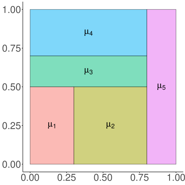
Figure 1: A binary decision tree $\mathbf{T}$ on $[0,1]^{2}$ with $5$ terminal nodes (left panel), and a regression tree function $g(\cdot;\mathbf{T},\mathcal{M})$ with $\mathcal{M}=\{\mu_{\ell}\}_{\ell=1}^{5}$ (right panel).

To avoid overfitting, a regularization prior is imposed on the model parameters. In particular, the prior takes the form $\pi\big{(}\{\mathbf{T}_{k},\mathcal{M}_{k}\}_{k=1}^{K}\big{)}=\prod_{k=1}^{K}\pi(\mathcal{M}_{k}\mid\mathbf{T}_{k})\pi(\mathbf{T}_{k})$. For the node parameters $\mathcal{M}_{k}$, conjugate normal priors are typically used to enable Gibbs sampling. The binary decision tree prior $\pi(\mathbf{T}_{k})$ is specified implicitly by the following tree-generating stochastic process. First, $\mathbf{T}_{k}$ is initialized with a single root node with depth $d=0$; the probability that a node at depth $d\geq 0$ splits (i.e., it is internal) is $p_{\text{split}}(d)$. For any internal node, its splitting rule is assigned by first sampling a splitting variable index $j$ uniformly from the available indices in $[p]$, and then sampling a splitting value $z$ uniformly from the available covariate values of the variable $\mathbf{x}(j)$. The splitting probability in Chipman et al. (1998, 2010) takes the form $p_{\mathrm{split}}(d)=a_{\mathrm{split}}(1+d)^{-b_{\mathrm{split}}}$, where $a_{\mathrm{split}}\in(0,1)$ and $b_{\mathrm{split}}\geq 0$ are hyperparameters. Apparently, this prior penalizes the splitting probabilities for nodes of large depths.

2.2 Functional BART via B-spline Representation

2.2.1 Functional Regression Tree Map

We first introduce a family of maps from $[0,1]^{p}$ to $L_{2}([0,1])$, termed as the functional regression tree maps. In particular, the response variable here is a real function, inherently existing in an infinite-dimensional space. Therefore, it is crucial to identify a suitable method for representing the functional data. Among various available approaches, the B-splines approach stands out due to its appealing theoretical properties and numerical advantages (de Boor, 1978; Unser et al., 1993).

The order-$q$ B-spline basis (de Boor, 1978) can be recursively defined as follows. Let $\{\xi_{j}\}_{j=1}^{J+q}$ be a knot sequence satisfying $\xi_{j+1}=\xi_{j}$ if $j\leq q-1$ or $j\geq J+1$, and $\xi_{j+1}>\xi_{j}$ otherwise. For $\underline{q}\leq q$, the B-spline basis functions $\{\phi_{j,\underline{q}}\}_{j=1}^{J+q-\underline{q}}$ of order $\underline{q}$ take the following form:

$$\phi_{j,\underline{q}}(t)=\left\{\begin{aligned} &\mathbb{I}_{[\xi_{j},\xi_{j+1})}(t),\quad\quad\underline{q}=1,\\ &\frac{t-\xi_{j}}{\xi_{j+\underline{q}-1}-\xi_{j}}\phi_{j,\underline{q}-1}(t)+\frac{\xi_{j+\underline{q}}-t}{\xi_{j+\underline{q}}-\xi_{j+1}}\phi_{j+1,\underline{q}-1}(t),\quad\underline{q}>1.\end{aligned}\right.$$ (2)

In the subsequent context, for simplicity, we may omit the order $q$ in the subscript of the B-spline basis functions.

Let $\{\phi_{j}\}_{j\in[J]}$ be a set of B-spline basis functions of order $q$ whose boundary knots are $\xi_{1}=0$ and $\xi_{J+q}=1$. Given a binary decision tree $\mathbf{T}$ with $L$ leaf nodes and node parameters $\mathcal{M}=\{\boldsymbol{\mu}_{1},\ldots,\boldsymbol{\mu}_{L}\}\subseteq\mathbb{R}^{J}$, we refer to the following map $\Xi_{\mathbf{T},\mathcal{M}}:[0,1]^{p}\to L_{2}([0,1])$ as a functional regression tree map:

$$\Xi_{\mathbf{T},\mathcal{M}}(\cdot)=\sum_{\ell=1}^{L}\boldsymbol{\phi}^{\mathsf{T}}\boldsymbol{\mu}_{\ell}\times\mathbb{I}_{D^{\ell}}(\cdot)=\sum_{\ell=1}^{L}\left[\sum_{j=1}^{J}\phi_{j}\boldsymbol{\mu}_{\ell}(j)\right]\times\mathbb{I}_{D^{\ell}}(\cdot),$$ (3)

where $\boldsymbol{\phi}=(\phi_{1},\phi_{2},\ldots,\phi_{J})^{\mathsf{T}}$ is the basis-function vector and $\mathcal{D}=\{D^{1},\ldots,D^{L}\}$ is the partition of $[0,1]^{p}$ induced by $\mathbf{T}$.

In the spirit of boosting, we define the functional additive regression tree map as follows. Let $\{\mathbf{T}_{k}\}_{k=1}^{K}$ denote a collection of $K\geq 1$ binary decision trees. For each $\mathbf{T}_{k}$ of $L_{k}$ leaf nodes, the induced partition is $\mathcal{D}_{k}=\{D_{k}^{\ell}\}_{\ell=1}^{L_{k}}$. Let $\mathcal{M}_{k}=\{\boldsymbol{\mu}_{k\ell}\}_{\ell=1}^{L_{k}}\subseteq\mathbb{R}^{J}$ be the node parameters associated with $\mathbf{T}_{k}$. By writing $\mathbb{T}=\{\mathbf{T}_{k}\}_{k=1}^{K}$ and $\mathbb{M}=\{\mathcal{M}_{k}\}_{k=1}^{K}$, the functional additive regression tree map is as follows:

$$\Xi_{\mathbb{T},\mathbb{M}}(\cdot)=\sum_{k=1}^{K}\Xi_{\mathbf{T}_{k},\mathcal{M}_{k}}(\cdot)=\sum_{k=1}^{K}\sum_{\ell=1}^{L_{k}}\boldsymbol{\phi}^{\mathsf{T}}\boldsymbol{\mu}_{k\ell}\times\mathbb{I}_{D_{k}^{\ell}}(\cdot).$$ (4)

We note that, although we focus on the axis-aligned partition induced by binary decision trees in this paper, the above treatment is generic and other space partitioning methods can be incorporated. Possible alternatives include random tessellation forests (Ge et al., 2019) and random spanning trees (Luo et al., 2021).

2.2.2 Prior Specification and Posterior Inference

According to the definition, the parameters involved in the functional additive regression tree map $\Xi_{\mathbb{T},\mathbb{M}}$ are $K$ binary decision trees $\{\mathbf{T}_{k}\}_{k=1}^{K}$ and $K$ sets of node parameters $\{\mathcal{M}_{k}\}_{k=1}^{K}$. To complete our Bayesian model, we need to specify the prior distributions of $\{\mathbf{T}_{k},\mathcal{M}_{k}\}_{k=1}^{K}$ and the noise variance $\sigma^{2}$.

In particular, the regularization prior of FBART is specified similarly to that of BART:

$$\pi\Big{(}\{\mathbf{T}_{k},\mathcal{M}_{k}\}_{k=1}^{K},\sigma^{2}\Big{)}=\pi(\sigma^{2})\prod_{k=1}^{K}\pi(\mathcal{M}_{k}\mid\mathbf{T}_{k})\pi(\mathbf{T}_{k}).$$ (5)

For the prior distributions of $\mathcal{M}_{k}$’s and $\sigma^{2}$, we use conjugate priors

$$\pi(\sigma^{2})\sim\nu\lambda/\chi^{2}_{\nu},\quad\pi\big{(}\mathcal{M}_{k}\mid\mathbf{T}_{k}\big{)}=\prod_{\ell=1}^{L_{k}}\mathcal{N}(\boldsymbol{\mu}_{k\ell};\boldsymbol{\mu}_{\mu},\mathbf{V}_{\mu}),$$ (6)

where $\chi^{2}_{\nu}$ stands for the Chi-square distribution with degrees of freedom $\nu$, and hyperparameters are $\boldsymbol{\mu}_{\mu}\in\mathbb{R}^{J}$, the covariance matrix $\mathbf{V}_{\mu}\in\mathbb{R}^{J\times J}$, $\lambda\in\mathbb{R}^{+}$, and $\nu\in\mathbb{N}^{+}$. For the prior distributions of $\mathbf{T}_{k}$’s, we employ the same tree prior described in Section 2.1 except for the splitting probability $p_{\text{split}}(d)$. Unlike the specification in Chipman et al. (1998, 2010), the splitting probability for constructing $\pi(\mathbf{T}_{k})$ takes the following form

$$p_{\text{split}}(d)=a\gamma^{d},$$ (7)

where $a\in(0,1]$ and $\gamma\in(0,1)$ are hyperparameters. This modification is motivated by Ročková and Saha (2019) to ensure that $\pi(\mathbf{T}_{k})$ exhibits certain tail behaviors.

We present the following Lemma 1 as the cornerstone for the subsequent posterior sampling algorithms. It basically shows that both the full conditional distributions of $\{\mathcal{M}_{k}\}$ and the marginal (conditional) likelihood over $\{\mathcal{M}_{k}\}$ have closed forms.

Lemma 1.

Consider the function-on-scalar regression problem in (1) with regression map $\Xi_{\mathbb{T},\mathbb{M}}$ and the FBART prior specified by (5)–(7). Let $\boldsymbol{\phi}(\mathbf{t}_{i})\in\mathbb{R}^{m_{i}\times J}$ denote the matrix of $\boldsymbol{\phi}$ evaluated at $\mathbf{t}_{i}$, whose $j$-th column is $(\phi_{j}(t_{i1}),\phi_{j}(t_{i2}),\ldots,\phi_{j}(t_{im_{i}}))^{\mathsf{T}}$, for $j\in[J]$. For each $k\in[K]$, let $\mathbf{T}_{(k)}=\{\mathbf{T}_{k^{\prime}}\}_{k^{\prime}\neq k}$, $\mathcal{M}_{(k)}=\{\mathbf{M}_{k^{\prime}}\}_{k^{\prime}\neq k}$, and define the partial residuals

$$\mathbf{r}_{i}=\mathbf{y}_{i}-\sum_{k^{\prime}=1,k^{\prime}\neq k}^{K}\Xi_{\mathbf{T}_{k^{\prime}},\mathcal{M}_{k^{\prime}}}(\mathbf{t}_{i};\mathbf{x}_{i}),\quad i=1,2,\ldots,n.$$

Then, it holds that

• The full conditional distribution of the node parameters $\mathcal{M}_{k}=\{\boldsymbol{\mu}_{k\ell}\}_{\ell=1}^{L_{k}}$ follows the normal distribution given below:

  $$\Pi_{n}\big{(}\mathcal{M}_{k}\mid\mathbf{y}_{1},\ldots,\mathbf{y}_{n},\mathbf{T}_{k},\mathbf{T}_{(k)},\mathcal{M}_{(k)},\sigma^{2}\big{)}=\prod_{\ell=1}^{L_{k}}\mathcal{N}(\boldsymbol{\mu}_{k\ell};\boldsymbol{\mu}_{\text{post}}^{k\ell},\mathbf{V}_{\text{post}}^{k\ell}),$$ (8)

  where

  $$\mathbf{V}_{\text{post}}^{k\ell}=\Big{[}\mathbf{V}_{\mu}^{-1}+\frac{1}{\sigma^{2}}\sum_{i:\mathbf{x}_{i}\in D_{k}^{\ell}}\boldsymbol{\phi}^{\mathsf{T}}(\mathbf{t}_{i})\boldsymbol{\phi}(\mathbf{t}_{i})\Big{]}^{-1}\ \ \textnormal{and}\ \ \boldsymbol{\mu}_{\text{post}}^{k\ell}=\mathbf{V}_{\text{post}}^{k\ell}\Big{[}\frac{1}{\sigma^{2}}\sum_{i:\mathbf{x}_{i}\in D_{k}^{\ell}}\boldsymbol{\phi}^{\mathsf{T}}(\mathbf{t}_{i})\mathbf{r}_{i}+\mathbf{V}_{\mu}^{-1}\boldsymbol{\mu}_{\mu}\Big{]}.$$ (9)

• Given other parameters, the marginal likelihood over $\mathcal{M}_{k}$ is

  $$p(\mathbf{y}_{1},\ldots,\mathbf{y}_{n}\mid\mathbf{T}_{k},\mathbf{T}_{(k)},\mathcal{M}_{(k)},\sigma^{2})=\prod_{\ell=1}^{L_{k}}p(\{\mathbf{r}_{i}\}_{i:\mathbf{x}_{i}\in D_{k}^{\ell}}\mid\sigma^{2}),$$

  where $p(\{\mathbf{r}_{i}\}_{i:\mathbf{x}_{i}\in D_{k}^{\ell}}\mid\sigma^{2})$ equals

  $$\frac{(2\pi\sigma^{2})^{-\frac{N_{k\ell}}{2}}|\mathbf{V}_{\mu}|^{-1/2}}{|\mathbf{V}_{\text{post}}^{k\ell}|^{-1/2}}\exp\Big{[}\frac{1}{2}(\boldsymbol{\mu}_{\text{post}}^{k\ell})^{\mathsf{T}}(\mathbf{V}_{\text{post}}^{k\ell})^{-1}\boldsymbol{\mu}_{\text{post}}^{k\ell}-\frac{1}{2\sigma^{2}}\sum_{i:\mathbf{x}_{i}\in D_{k}^{\ell}}\mathbf{r}_{i}^{\mathsf{T}}\mathbf{r}_{i}-\frac{1}{2}\boldsymbol{\mu}_{\mu}^{\mathsf{T}}\mathbf{V}_{\mu}^{-1}\boldsymbol{\mu}_{\mu}\Big{]},$$ (10)

  and $N_{k\ell}=\sum_{i:\mathbf{x}_{i}\in D_{k}^{\ell}}m_{i}$ is the total number of observations in the $\ell$-th subregion induced by $\mathbf{T}_{k}$.

To conduct posterior inference for FBART through Markov chain Monte Carlo (MCMC), we propose a Bayesian backfitting algorithm by tailoring the existing implementations of BART. The conjugate Gibbs sampling is used for updating $\sigma^{2}$ and $\{\mathcal{M}_{k}\}_{k=1}^{K}$, while the Metropolis–Hastings (MH) updates are employed for updating $\{\mathbf{T}_{k}\}_{k=1}^{K}$ . Specifically, the proposal distribution $q(\mathbf{T},\mathbf{T}^{*})$ includes four moves: Grow, Prune, Change and Prior, following the R packages bartMachine (Kapelner and Bleich, 2016) and SoftBART (Linero and Yang, 2018). The proposed MCMC procedure is summarized in Algorithm 1. Additional implementation details and hyperparameter specifications are given in Section S.1 of the Supplementary Materials.

Algorithm 1 Bayesian backfitting MCMC algorithm for FBART

Input: Data $\big{\{}(\mathbf{x}_{i},\{Y_{i}(t_{ij})\}_{j=1}^{m_{i}})\big{\}}_{i=1}^{n}$; B-splines $\{\boldsymbol{\phi}_{j}\}_{j=1}^{J}$; Hyperparameters $(K,\boldsymbol{\mu}_{\mu},\mathbf{V}_{\mu},\nu,\lambda,a,\gamma)$; Number of iterations $\text{MC}_{\text{iter}}$.

Result: Posterior samples.

for $i_{\text{iter}}\in[\text{MC}_{\text{iter}}]$ do

    for $k\in[K]$ do

       Calculate the partial residuals $\mathbf{r}_{i}=\mathbf{y}_{i}-\sum_{k^{\prime}=1,k^{\prime}\neq k}^{K}\Xi_{\mathbf{T}_{k^{\prime}},\mathcal{M}_{k^{\prime}}}(\mathbf{t}_{i};\mathbf{x}_{i})$ for $i=1,2,\ldots,n$. 1. Update $\mathbf{T}_{k}$: (i). Sample a new $\mathbf{T}^{*}_{k}$ from the proposal distribution $q(\mathbf{T}_{k},\mathbf{T}^{*}_{k})$. (ii). Accept the new sample and update $\mathbf{T}_{k}=\mathbf{T}^{*}_{k}$ with probability

$$\alpha\left(\mathbf{T}_{k},\mathbf{T}^{*}_{k}\right)=\min\left\{\frac{q\left(\mathbf{T}_{k}^{*},\mathbf{T}_{k}\right)}{q\left(\mathbf{T}_{k},\mathbf{T}_{k}^{*}\right)}\frac{p\big{(}\mathbf{y}_{1},\ldots,\mathbf{y}_{n}\mid\mathbf{T}_{k}^{*},\mathbf{T}_{(k)},\mathcal{M}_{(k)},\sigma^{2}\big{)}\pi\left(\mathbf{T}_{k}^{*}\right)}{p\big{(}\mathbf{y}_{1},\ldots,\mathbf{y}_{n}\mid\mathbf{T}_{k},\mathbf{T}_{(k)},\mathcal{M}_{(k)},\sigma^{2}\big{)}\pi\left(\mathbf{T}_{k}\right)},\quad 1\right\},$$ (11)

where the marginal likelihoods $p\big{(}\mathbf{y}_{1},\ldots,\mathbf{y}_{n}\mid\mathbf{T}_{k}^{*},\mathbf{T}_{(k)},\mathcal{M}_{(k)},\sigma^{2}\big{)}$ and $p\big{(}\mathbf{y}_{1},\ldots,\mathbf{y}_{n}\mid\mathbf{T}_{k},\mathbf{T}_{(k)},\mathcal{M}_{(k)},\sigma^{2}\big{)}$ are calculated according to Equation (10). 2. Update $\mathcal{M}_{k}$: For each $\ell\in[L_{k}]$,

$$\boldsymbol{\mu}_{k\ell}\sim\mathcal{N}(\boldsymbol{\mu}_{\text{post}}^{k\ell},\mathbf{V}_{\text{post}}^{k\ell}),$$ (12)

where $\boldsymbol{\mu}_{\text{post}}^{k\ell}$ and $\mathbf{V}_{\text{post}}^{k\ell}$ are calculated according to Equation (9).

    end for

   3. Update $\sigma^{2}$:

$$\sigma^{2}\sim\mathrm{InvGamma}\Big{(}\frac{\nu+N_{n}}{2},\quad\frac{\lambda\nu+\sum_{i=1}^{n}\|\mathbf{y}_{i}-\Xi_{\mathbb{T},\mathbb{M}}(\mathbf{t}_{i};\mathbf{x}_{i})\|_{2}^{2}}{2}\Big{)},$$ (13)

where $\mathrm{InvGamma}(a,b)$ stands for an inverse gamma distribution with density $p(x)\propto x^{-a-1}\exp(-b/x)$.

end for

3 Shape-Constrained FBART (S-FBART)

In this section, we extend our proposed FBART to its shape-constrained version that incorporates the prior knowledge of functional responses. By leveraging the properties of B-splines, we can manipulate the spline coefficient vector to control the shape of their linear combination (e.g., Abraham and Khadraoui, 2015; Pya and Wood, 2015; Wang and Yan, 2021). Here, we consider the commonly used shape constraints of response curves, including positivity, monotonicity, and convexity. The following Lemma 2 shows how to impose these shape constraints by imposing linear constraints on spline coefficients.

Lemma 2.

Let $\{\phi_{j}\}_{j=1}^{J}$ denote the B-spline basis functions with order $q\geq 1$ and knots $\xi_{1}=\xi_{2}=\ldots=\xi_{q}<\xi_{q+1}<\ldots<\xi_{J}<\xi_{J+1}=\xi_{J+2}=\ldots=\xi_{J+q}$. Given a basis coefficient vector $\boldsymbol{\mu}\in\mathbb{R}^{J}$ such that $\mathbf{D}\boldsymbol{\mu}\geq\mathbf{0}$ for some matrix $\mathbf{D}\in\mathbb{R}^{J^{\prime}\times J}$ with $J^{\prime}\leq J$, we have

• $\boldsymbol{\phi}^{\mathsf{T}}\boldsymbol{\mu}$ is positive (non-negative) if $\mathbf{D}=\mathbf{I}_{J}$;

• $\boldsymbol{\phi}^{\mathsf{T}}\boldsymbol{\mu}$ is increasing if the $j$-th row of $\mathbf{D}\in\mathbb{R}^{(J-1)\times J}$ is

  $$(0,\ldots,0,-1,1,0,\ldots,0),$$

  where the indices of nonzero entries are $j$ and $j+1$, for $j\in[J-1]$;

• $\boldsymbol{\phi}^{\mathsf{T}}\boldsymbol{\mu}$ is convex if the $j$-th row is of $\mathbf{D}\in\mathbb{R}^{(J-2)\times J}$ is

  $$\Big{(}0,\ldots,0,(\xi_{j+q}-\xi_{j+1})^{-1},-(\xi_{j+q}-\xi_{j+1})^{-1}-(\xi_{j+q+1}-\xi_{j+2})^{-1},(\xi_{j+q+1}-\xi_{j+2})^{-1},0,\ldots,0\Big{)},$$

  where the indices of nonzero entries are $j$, $j+1$ and $j+2$, for $j\in[J-2]$.

We refer to the matrix $\mathbf{D}$ in Lemma 2 as the constraint matrix for a given shape constraint. By combining different constraint matrices, we can impose more complex shape constraints on the fitted function $\boldsymbol{\phi}^{\mathsf{T}}\boldsymbol{\mu}$, such as both monotonicity and convexity. See Section S.1.4 of the Supplementary Materials for more details.

Next, we discuss the posterior inference of the S-FBART model. Based on the above discussion, we can extend the prior distribution of FBART given in Section 2.2.2 to the one ensuring a required shape constraint. This extension is based on a constrained version of normal distributions. Given a certain shape constraint in Lemma 2 and the corresponding constraint matrix $\mathbf{D}$, we say a random vector $\boldsymbol{\mu}\in\mathbb{R}^{J}$ follows a shape-constrained normal distribution $\mathcal{N}^{\mathbf{D}}(\boldsymbol{\mu}_{\mu},\mathbf{V}_{\mu})$, if its density has the following form:

$$p(\boldsymbol{\mu})=\frac{1}{\sqrt{(2\pi)^{J}|\mathbf{V}_{\mu}|}C_{\mathbf{D}}(\boldsymbol{\mu}_{\mu},\mathbf{V}_{\mu})}\exp\Big{[}-\frac{1}{2}(\boldsymbol{\mu}-\boldsymbol{\mu}_{\mu})^{\mathsf{T}}\mathbf{V}_{\mu}^{-1}(\boldsymbol{\mu}-\boldsymbol{\mu}_{\mu})\Big{]}\mathbb{I}_{\{\boldsymbol{\mu}:\mathbf{D}\boldsymbol{\mu}\geq\mathbf{0}\}}(\boldsymbol{\mu}),$$ (14)

where $C_{\mathbf{D}}(\boldsymbol{\mu}_{\mu},\mathbf{V}_{\mu})$ is a normalizing constant depending on the mean vector $\boldsymbol{\mu}_{\mu}$ and covariance matrix $\mathbf{V}_{\mu}$. The shape-constrained normal distribution is closely related to the truncated normal distribution. In particular, let $\bar{\mathbf{D}}\in\mathbb{R}^{J\times J}$ denote an invertible matrix whose first $J^{\prime}$ rows are $\mathbf{D}$. By writing $\boldsymbol{\eta}=\bar{\mathbf{D}}\boldsymbol{\mu}$, we have

$$\boldsymbol{\mu}\sim\mathcal{N}^{\mathbf{D}}(\boldsymbol{\mu}_{\mu},\mathbf{V}_{\mu})\Longleftrightarrow\boldsymbol{\eta}\sim\mathcal{N}^{+}_{1:J^{\prime}}(\bar{\mathbf{D}}\boldsymbol{\mu}_{\mu},\bar{\mathbf{D}}\mathbf{V}_{\mu}\bar{\mathbf{D}}^{\mathsf{T}}),$$ (15)

where $\mathcal{N}^{+}_{1:J^{\prime}}$ denotes the truncated normal distribution with positivity constraints on the first $J^{\prime}$ entries.

Let $\pi^{\mathbf{D}}(\cdot)$ denote the prior of S-FBART with a constraint matrix $\mathbf{D}$ corresponding to a certain shape constraint given in Lemma 2. The prior $\pi^{\mathbf{D}}(\cdot)$ is defined by simply replacing the priors of $\{\mathcal{M}_{k}\}$ in FBART with shape-constrained normal distributions:

$$\pi^{\mathbf{D}}\Big{(}\{\mathbf{T}_{k},\mathcal{M}_{k}\}_{k=1}^{K},\sigma^{2}\Big{)}=\pi(\sigma^{2})\prod_{k=1}^{K}\Big{[}\prod_{\ell=1}^{L_{k}}\mathcal{N}^{\mathbf{D}}(\boldsymbol{\mu}_{k\ell};\boldsymbol{\mu}_{\mu},\mathbf{V}_{\mu})\Big{]}\pi(\mathbf{T}_{k}).$$ (16)

Corollary 1.

In S-FBART, the induced prior and posterior distributions of $\Xi(\mathbf{x})$ satisfy the specified shape constraint for all $\mathbf{x}\in[0,1]^{p}$.

Similar to Lemma 1, we present some basic results for S-FBART in Lemma 3. To sample from the posterior, we again use Algorithm 1 with two modifications: i) To update $\mathbf{T}_{k}$, the marginal likelihood in Equation (11) is calculated according to Equation (18) instead of Equation (10); and ii) to update $\mathcal{M}_{k}$ in Equation (12), we sample from the shape-constrained normal distribution $\boldsymbol{\mu}_{k\ell}\sim\mathcal{N}^{\mathbf{D}}(\boldsymbol{\mu}_{\text{post}}^{k\ell},\mathbf{V}_{\text{post}}^{k\ell})$, for $\ell\in[L_{k}]$.

Lemma 3.

Given a certain shape constraint in Lemma 2 and the associated constraint matrix $\mathbf{D}$, consider the function-on-scalar regression problem in (1) with regression map $\Xi_{\mathbb{T},\mathbb{M}}$ and the S-FBART prior specified in Equation (16). For each $k\in[K]$, we have:

• The full conditional distribution of the node parameters $\mathcal{M}_{k}=\{\boldsymbol{\mu}_{k\ell}\}_{\ell=1}^{L_{k}}$ is

  $$\Pi_{n}\big{(}\mathcal{M}_{k}\mid\mathbf{y}_{1},\ldots,\mathbf{y}_{n},\mathbf{T}_{k},\mathbf{T}_{(k)},\mathcal{M}_{(k)},\sigma^{2}\big{)}=\prod_{\ell=1}^{L}\mathcal{N}^{\mathbf{D}}(\boldsymbol{\mu}_{k\ell};\boldsymbol{\mu}_{\text{post}}^{k\ell},\mathbf{V}_{\text{post}}^{k\ell}),$$ (17)

  where $\boldsymbol{\mu}_{\text{post}}^{k\ell}$ and $\mathbf{V}_{\text{post}}^{k\ell}$ are given in Equation (9);

• The marginal likelihood $p^{\mathbf{D}}(\mathbf{y}_{1},\ldots,\mathbf{y}_{n}\mid\mathbf{T}_{k},\mathbf{T}_{(k)},\mathcal{M}_{(k)},\sigma^{2})$ for S-FBART is

  $$p(\mathbf{y}_{1},\ldots,\mathbf{y}_{n}\mid\mathbf{T}_{k},\mathbf{T}_{(k)},\mathcal{M}_{(k)},\sigma^{2})\times\prod_{\ell=1}^{L_{k}}\frac{C_{\mathbf{D}}(\boldsymbol{\mu}_{\text{post}}^{k\ell},\mathbf{V}_{\text{post}}^{k\ell})}{C_{\mathbf{D}}(\boldsymbol{\mu}_{\mu},\mathbf{V}_{\mu})},$$ (18)

  where $p(\mathbf{y}_{1},\ldots,\mathbf{y}_{n}\mid\mathbf{T}_{k},\mathbf{T}_{(k)},\mathcal{M}_{(k)},\sigma^{2})$ is given in Equation (10).

As shown in Equation (15), the implementation of S-FBART involves sampling from truncated normal distributions and evaluating multivariate normal probabilities $C_{\mathbf{D}}(\cdot,\cdot)$. Sampling from a truncated normal distribution can be achieved through methods such as rejection sampling or Gibbs sampling (e.g., Kotecha and Djuric, 1999), while normal integrals can be numerically computed using Monte Carlo algorithms (e.g., Genz and Bretz, 2009). Recently, Botev (2017) introduced a minimax tilting method that offers exact sampling and accurate integral calculation for truncated normal distributions. We adopt this method in our implementation and find it works satisfactorily. Finally, it is worth noting that we focus on the case of moderately large dimension $J$ in this paper, which is typically around $10$. Hence, our sampling algorithms do not involve calculating high-dimensional truncated normal densities.

4 Posterior Concentration Results

In this section, we investigate the theoretical properties of FBART and S-FBART. We will show the proposed methods can provide consistent estimation and derive their posterior contraction rates.

In our setup, the observations $\big{\{}(\mathbf{x}_{i},\{Y_{i}(t_{ij})\}_{j=1}^{m_{i}})\big{\}}_{i=1}^{n}$ are generated according to the FOSR model in (1). We assume the true map $\Xi_{0}$ lives in the following space:

$$\mathcal{HC}^{\alpha,\beta}:=\Big{\{}\Xi:[0,1]^{p}\to C^{\alpha}[0,1];\ \ \sup_{\mathbf{x}\neq\mathbf{x}^{\prime}}\frac{\|\Xi(\mathbf{x})-\Xi(\mathbf{x}^{\prime})\|_{C^{\alpha}}}{\|\mathbf{x}-\mathbf{x}^{\prime}\|_{2}^{\beta}}<\infty\Big{\}},$$ (19)

where $\alpha>0$, $\beta\in(0,1]$, and $\|\cdot\|_{C^{\alpha}}$ denotes the Hölder norm of order $\alpha$. The convergence results will be derived with respect to the following metric:

$$d^{2}_{n}(\Xi,\Xi^{\prime}):=\frac{1}{N_{n}}\sum_{i=1}^{n}\|\Xi(\mathbf{t}_{i};\mathbf{x}_{i})-\Xi^{\prime}(\mathbf{t}_{i};\mathbf{x}_{i})\|_{2}^{2},$$ (20)

where $\Xi$ and $\Xi^{\prime}$ are two regression maps. Recall that $N_{n}=\sum_{i=1}^{n}m_{i}$, and $m_{i}$ is the number of observed points for subject $i$. Throughout this section, the error variance $\sigma^{2}$ is fixed at $1$ for simplicity, and relaxation to an unknown $\sigma^{2}$ is possible (Ghosal and Van der Vaart, 2017). We allow each $m_{i}$ to (implicitly) depend on $n$, and assume there exists a positive constant $\xi<\infty$ such that $(\max_{i=1}^{n}m_{i})/(\min_{i=1}^{n}m_{i})\leq\xi$ for all $n$. The covariate dimension $p$ is considered to be fixed for simplicity, and extension to high-dimensional regression is possible by introducing a sparsity-inducing prior (e.g., Linero, 2018). For any two sequences $A_{n}$ and $B_{n}$, we write $A_{n}\lesssim B_{n}$ if $A_{n}\leq cB_{n}$ for some constant $c>0$ independent of $n$, $A_{n}\gtrsim B_{n}$ if $B_{n}\lesssim A_{n}$, and $A_{n}\asymp B_{n}$ if $A_{n}\lesssim B_{n}$ and $B_{n}\lesssim A_{n}$.

Our proof focuses on the space partition induced by k-d trees. We call a binary decision tree $\mathbf{T}$ a k-d tree (Ročková and Van der Pas, 2020), if it satisfies the following properties: 1) All the terminal nodes have the same depth; 2) the splitting variable cycles over $[p]$, and the internal nodes at the same depth share the same splitting variable; 3) the splitting value at each node is the median observed value in the node along the splitting variable. Based on the definition of the k-d tree, after $s$ rounds of splitting cycles, the resulting k-d tree has $L=2^{sp}$ terminal nodes and each terminal node contains at least $\lfloor n/L\rfloor$ observations. The induced partition $\mathcal{D}=\{D^{1},\ldots,D^{L}\}$ by a k-d tree is referred to as a k-d tree partition.

To proceed, we assume the design points $\{\mathbf{x}_{i}\}_{i=1}^{n}$ are “regular” in the sense defined in Condition 1. Intuitively speaking, Condition 1 requires the design points $\{\mathbf{x}_{i}\}_{i=1}^{n}$ to be approximately uniform in the predictor space. For example, this condition is satisfied if $\{\mathbf{x}_{i}\}$ are on a regular grid of $[0,1]^{p}$.

Condition 1.

There exists a constant $M>0$, such that for any $s\geq 1$, the k-d tree partition $\mathcal{D}=\{D^{1},\ldots,D^{L}\}$ with $L=2^{sp}$ satisfies

$$\max_{1\leq\ell\leq L}\mathrm{diam}(D^{\ell})\leq M\sum_{\ell=1}^{L}\frac{n_{\ell}}{n}\mathrm{diam}(D^{\ell}),$$ (21)

where $\mathrm{diam}(D^{\ell})=\max\limits_{\mathbf{x}_{i},\mathbf{x}_{i^{\prime}}\in\mathcal{D}^{\ell}}\|\mathbf{x}_{i}-\mathbf{x}_{i^{\prime}}\|_{2}$ and $n_{\ell}=\sum\limits_{i=1}^{n}\mathbb{I}_{D^{\ell}}(\mathbf{x}_{i})$.

The following Lemma 4 gives the error bound of the k-d tree map for approximating the true functional regression map.

Lemma 4.

Assume $\Xi_{0}\in\mathcal{HC}^{\alpha,\beta}$ for some $\alpha>0$ and $\beta\in(0,1]$, and $\{\mathbf{x}_{i}\}_{i=1}^{n}$ satisfies Condition 1. Let $\boldsymbol{\phi}=(\phi_{1},\ldots,\phi_{J})^{\mathsf{T}}$ be a set of B-spline basis functions of order $q\geq\alpha$ with equally spaced knots. Then, for any k-d tree $\mathbf{T}$ with $L$ terminal nodes, there exists a set of node parameters $\widehat{\mathcal{M}}$ such that the tree-structured step map $\widehat{\Xi}=\Xi_{\mathbf{T},\widehat{\mathcal{M}}}$ satisfies

$$d_{n}(\widehat{\Xi},\Xi_{0})\lesssim J^{-\alpha}+L^{-\beta/p}.$$ (22)

Our posterior convergence results rely on three conditions to hold (e.g., see Ghosal and van der Vaart, 2007; Ročková and Van der Pas, 2020), which are presented in detail in Section S.4 of the Supplementary Materials. Specifically, let $\mathcal{G}=\{\sum_{k=1}^{K}\Xi_{\mathbf{T}_{k},\mathcal{M}_{k}}\}$ denote the space of all functional additive regression tree maps; the primary challenges for verifying these conditions are to derive the prior concentration rate at $\Xi_{0}$, and to properly construct subsets $\mathcal{G}_{n}\subseteq\mathcal{G}$ that can well approximate $\mathcal{G}$ with relatively low complexity.

The following main theorem shows the posterior consistency of our proposed FBART estimator:

Theorem 1.

Assume $\Xi_{0}\in\mathcal{HC}^{\alpha,\beta}$ for some $\alpha>0$ and $\beta\in(0,1]$, and Condition 1 is satisfied. Let $J_{n}\asymp N_{n}^{\frac{\beta}{\alpha(2\beta+p)+\beta}}$ and the space $\mathcal{G}$ be endowed with the FBART prior specified as follows:

$$\pi_{n}\Big{(}\{\mathbf{T}_{k},\mathcal{M}_{k}\}_{k=1}^{K}\Big{)}=\prod_{k=1}^{K}\pi_{n}(\mathbf{T}_{k})\prod_{\ell=1}^{L_{k}}\mathcal{N}(\boldsymbol{\mu}_{k\ell};\mathbf{0},\mathbf{I}_{J}/K),$$ (23)

where $\pi_{n}(\mathbf{T})$ follows the prior of decision tree in Chipman et al. (2010) with $p_{\mathrm{split}}(d)=\gamma^{J_{n}\log(J_{n})+d}$ for some $\gamma\in(0,\frac{1}{2})$. Then with $\varepsilon_{n}=N_{n}^{-\frac{\alpha\beta}{\alpha(2\beta+p)+\beta}}\log^{1/2}N_{n}$, we have

$$\Pi_{n}\Big{(}\Xi\in\mathcal{G}:d_{n}(\Xi,\Xi_{0})>C_{n}\varepsilon_{n}\mid Y_{1}(\mathbf{t}_{1}),\ldots,Y_{n}(\mathbf{t}_{n})\Big{)}\longrightarrow 0$$ (24)

for any $C_{n}\to\infty$ in $\mathbb{P}^{n}_{\Xi_{0}}$-probability, as $n\to\infty$.

For the shape-constrained FBART proposed in Section 3, we have similar convergence results. We first investigate how the linear constraint in Lemma 2 affects the approximation power of B-spline functions.

Lemma 5.

We define a function $Y(t)\in C^{\alpha}[0,1]$ to be $\kappa$-strictly shape-constrained for some $\kappa>0$, if $Y(t)$ satisfies one of the following conditions:

• $Y(t)$ is strictly positive, i.e., $Y(t)\geq\kappa$ for all $t\in[0,1]$;

• $Y(t)$ is strictly increasing with $\alpha>1$, i.e., $\frac{\mathrm{d}Y(t)}{\mathrm{d}t}\geq\kappa$ for all $t\in[0,1]$;

• $Y(t)$ is strictly convex with $\alpha>2$, i.e., $\frac{\mathrm{d}^{2}}{\mathrm{d}t^{2}}Y(t)\geq\kappa$ for all $t\in[0,1]$.

Let $\boldsymbol{\phi}=(\phi_{1},\ldots,\phi_{J})^{\mathsf{T}}$ be a set of B-spline basis functions of order $q\geq\alpha$ with equally spaced knots, and $\mathbf{D}$ be the associated constraint matrix for $Y(t)$. Then, for large enough $J$, we have

$$\inf_{\boldsymbol{\mu}\in\mathbb{R}^{J}:\mathbf{D}\boldsymbol{\mu}\geq\mathbf{0}}\|\boldsymbol{\phi}^{\mathsf{T}}\boldsymbol{\mu}-Y\|_{\infty}\lesssim J^{-\alpha}.$$ (25)

Lemma 5 shows that the approximation error of the constrained B-splines representation is of the same order as that of the unconstrained one, as long as the target function is strictly shape-constrained. When the shape constraints are not strict, the corresponding best approximation error can be sub-optimal (De Boor and Daniel, 1974). The following corollary establishes the consistency of our proposed S-FBART estimator for shape-constrained functional responses.

Corollary 2.

Under the same conditions and settings in Theorem 1, suppose in addition that there exists $\kappa>0$ such that $\Xi_{0}(\mathbf{x})$ is $\kappa$-strictly shape-constrained for all $\mathbf{x}\in[0,1]^{p}$ with constraint matrix $\mathbf{D}$. Then, the claim in Theorem 1 still holds for the posterior distribution of S-FBART when the space $\mathcal{G}$ is endowed with the S-FBART prior specified below:

$$\pi_{n}^{\mathbf{D}}\Big{(}\{\mathbf{T}_{k},\mathcal{M}_{k}\}_{k=1}^{K}\Big{)}=\prod_{k=1}^{K}\pi_{n}(\mathbf{T}_{k})\prod_{\ell=1}^{L_{k}}\mathcal{N}^{\mathbf{D}}(\boldsymbol{\mu}_{k\ell};\mathbf{0},\mathbf{I}_{J}/K),$$ (26)

where $\pi_{n}(\mathbf{T}_{k})$ is the tree prior specified in Theorem 1.

5 Numerical Studies

5.1 Simulation Setup

First, we evaluate the performance of the proposed FBART and S-FBART methods through simulation experiments. We consider the model given in (1) with $p=2$ covariates and functional responses defined on $[0,1]$. We independently sample $n=400$ covariate vectors uniformly over the covariate space. Each curve $\{Y_{i}(t_{ij})\}_{j\in[m_{i}]}$ contains $m_{i}=m=20$ observations at a regular grid of sampling points, $\{t_{ij}=\frac{j}{21}:j\in[m_{i}]\}$. We use $J=10$ cubic B-spline basis functions with equally spaced knots to approximate the true response function. We consider different noise levels with $\sigma\in\{0.1,1\}$. For the true regression map, we consider the following three cases:

Case 1: A piece-wise constant map

$$\Xi_{1}(t;\mathbf{x})=\big{\{}1+\mathbb{I}_{[0,0.5]}(\mathbf{x}(1))\big{\}}\tan\Big{(}4\pi\big{[}t+t^{2\mathbb{I}_{[0,0.5]}(\mathbf{x}(2))}-1\big{]}/9\Big{)};$$ (27)

Case 2: A map involving both smooth and non-smooth parts:

$$\Xi_{2}(t;\mathbf{x})=\frac{4\mathbf{x}(1)+1}{\mathbf{x}(2)+2}t+2\big{\{}\mathbf{x}(2)\mathbb{I}_{[0,0.5]}(\mathbf{x}(1))+\mathbf{x}(2)\big{\}}\tan\Big{(}4\pi\big{[}t+t^{4\mathbf{x}(2)}-1\big{]}/9\Big{)};$$ (28)

Case 3: A linear map:

$$\Xi_{3}(t;\mathbf{x})=\mathbf{x}(1)+\mathbf{x}(2)+\big{(}1+2\mathbf{x}(1)+4\mathbf{x}(2)\big{)}\Phi^{-1}(t),$$ (29)

where $\Phi^{-1}(\cdot)$ is the quantile function of the standard normal distribution. Note that in all three cases, the true regression map is monotonically increasing in $t$ for any $\mathbf{x}\in[0,1]^{2}$.

We compare the proposed FBART and S-FBART with several state-of-the-art competitive methods, including the classical BART (Chipman et al., 2010), the monotone BART (mBART, Chipman et al., 2022), the Bayesian FOSR method (BFOSR, Kowal and Bourgeois, 2020), and the local linear regression methods with functional responses (LLR, e.g., Petersen and Müller, 2019; Fan and Müller, 2022). For BART and mBART, we treat $Y_{i}(t_{ij})$ as the response value with the covariate vector $(t_{ij},\mathbf{x}_{i}^{\mathsf{T}})^{\mathsf{T}}$ of dimension $(p+1)$; and a monotonically increasing constraint in $t$ is imposed for mBART. For the proposed S-FBART method, we use the constraint matrix $\mathbf{D}$ corresponding to the monotonically increasing constraint defined in Lemma 5. The hyperparameters in the above approaches, if not specified, are chosen according to their respective default settings. For all the additive tree models, we set $K=20$. For LLR, we use the normal kernel function, with the bandwidth chosen to minimize the in-sample root-mean-squared error.

The prediction performance of different methods is quantified by three metrics. In particular, for each simulation setup, we independently generate $n^{*}=400$ test data following the respective data-generating process. The first metric is the root mean squared prediction errors (RMSPE) defined as $\text{RMSPE}=\sqrt{\frac{1}{mn^{*}}\sum_{i=1}^{n^{*}}\|\hat{\Xi}(\mathbf{t}^{*}_{i};\mathbf{x}^{*}_{i})-\Xi_{0}(\mathbf{t}^{*}_{i};\mathbf{x}^{*}_{i})\|_{2}^{2}}$, where $\mathbf{x}^{*}_{i}$ and $\mathbf{t}^{*}_{i}$ are the covariate vector and sampling points for the test data, respectively; for Bayesian approaches, we use the posterior mean for point estimation. In addition, we calculate the pointwise posterior $95\%$ credible interval for uncertainty quantification. The accuracy of the credible interval is evaluated via the mean negatively oriented interval score (MIS, Gneiting and Raftery, 2007), defined as $\text{MIS}=\frac{1}{mn^{*}}\sum_{i=1}^{n^{*}}\sum_{j=1}^{m_{i}}\Big{[}\hat{U}_{ij}-\hat{L}_{ij}+\frac{2}{5\%}\inf_{\eta\in[\hat{L}_{ij},\hat{U}_{ij}]}|\Xi_{0}(t^{*}_{ij};\mathbf{x}^{*}_{i})-\eta|\Big{]}$, where $\hat{U}_{ij}$ and $\hat{L}_{ij}$ are the $97.5\%$-quantile and $2.5\%$-quantile of the posterior samples of $\Xi(t^{*}_{ij};\mathbf{x}^{*}_{i})$, respectively; note that for the frequentist approach LLR, MIS is calculated by setting $\hat{U}_{ij}=\hat{L}_{ij}=\hat{\Xi}(t^{*}_{ij};\mathbf{x}^{*}_{i})$. Last, we use the mean continuous ranked probability score (MCRPS, Gneiting and Raftery, 2007) metric to evaluate the performance of probabilistic prediction. For all three metrics, a lower value indicates a better performance.

5.2 Simulation Results

The average RMSPE, MIS, and MCRPS values (over $20$ replicates) for all methods are shown in Table 1. For each metric, the first two best results are shown in bold. For both Case 1 and Case 2, where the true relationship between the functional response and the covariate exhibits non-linearity and lack of smoothness, our proposed FBART and S-FBART methods consistently outperform other methods in terms of prediction performance and uncertainty quantification. This is not very surprising because FBART and S-FBART account for both the functional nature of the responses and the non-linearity of the true regression map. The BART and mBART methods outperform BFOSR and LLR, which assume a linear relationship between the response and covariates, but they cannot capture the functional structure of the responses well, thus leading to inferior prediction results to those of FBART and S-FBART. For Case 3, where a linear regression map is assumed, both BFOSR and LLR outperform other methods. This outcome aligns with our expectations, since these two methods are specifically designed for (locally) linear regression maps. However, it is noteworthy that FBART and S-FBART still manage to achieve MISs and MCRPSs that are comparable to those of linear models, especially when the noise level is high ($\sigma=1$).

We note that across all simulation scenarios, FBART and S-FBART consistently outperform BART and mBART in terms of all three evaluation metrics. This superior performance can be attributed to the spline modeling of functional data employed by FBART and S-FBART, which effectively captures the inherent functional nature of the responses.

Table 1: Comparison results of different methods in terms of three metrics.

$\sigma$	Case	Metric	FBART	S-FBART	BART	mBART	BFOSR	LLR
$\sigma=1$	case 1	RMSPE	0.168	0.184	$0.473$	$0.306$	$0.893$	$0.529$
		MIS	0.577	0.899	$6.431$	$3.581$	$5.987$	$14.401$
		MCRPS	0.573	0.575	$0.622$	$0.588$	$0.771$	$0.641$
	case 2	RMSPE	0.229	0.215	$0.842$	$0.443$	$0.806$	$0.368$
		MIS	1.051	1.011	$14.616$	$8.342$	$10.780$	$9.517$
		MCRPS	0.580	0.578	$0.733$	$0.616$	$0.888$	$0.602$
	case 3	RMSPE	$0.182$	$0.168$	$0.625$	$0.281$	0.049	0.083
		MIS	0.926	0.923	$11.175$	$4.949$	${1.434}$	${2.609}$
		MCRPS	$0.575$	$0.574$	$0.668$	$0.587$	0.567	0.568
$\sigma=0.1$	case 1	RMSPE	0.165	0.176	$0.494$	$0.282$	$0.890$	$0.780$
		MIS	0.482	0.554	$8.715$	$3.980$	$7.160$	$9.347$
		MCRPS	0.073	0.076	$0.239$	$0.118$	$0.512$	$0.248$
	case 2	RMSPE	0.143	0.150	$0.811$	$0.393$	$0.803$	$0.294$
		MIS	0.742	0.741	$17.486$	$8.799$	$3.989$	$4.584$
		MCRPS	0.093	0.095	$0.453$	$0.206$	$0.401$	$0.130$
	case 3	RMSPE	$0.048$	$0.042$	$0.584$	$0.192$	0.007	0.008
		MIS	$0.284$	$0.313$	$14.061$	$5.209$	0.133	0.261
		MCRPS	$0.064$	$0.064$	$0.365$	$0.119$	0.057	0.057

Next, we compare FBART and BART with their respective shape-constrained counterparts. We observe significant improvements when transitioning from BART to mBART across all scenarios. On the other hand, S-FBART yields results that are comparable to those of FBART. A possible explanation is that incorporating the shape information (i.e., monotonicity) is particularly beneficial for BART, since it does not make use of the functional structure of the responses.

To further study the impact of the shape-constrained inference, we examine the performance of FBART and S-FBART under Case 2 with different noise levels $\sigma\in\{0.1,0.5,1,2\}$. In Fig. 2, we present ratios of the three metrics between FBART and S-FBART using side-by-side boxplots. We can see that S-FBART is superior over BART at moderate noise levels (e.g., $\sigma=0.5$ or $1$), while delivering comparable results when the noise level is either too small or too large. This may be because when the noise level is too small, the responses already contain sufficient information on inferring the shape so that further incorporating the shape constraint in the model does not help to improve the prediction results. On the other hand, when the noise level is too large, although S-FBART can stabilize the prediction, adding the shape constraint to the inference increases the prediction bias in the meantime. Additional numerical results and further discussion are deferred to Section S.2.2 in the Supplementary Materials.

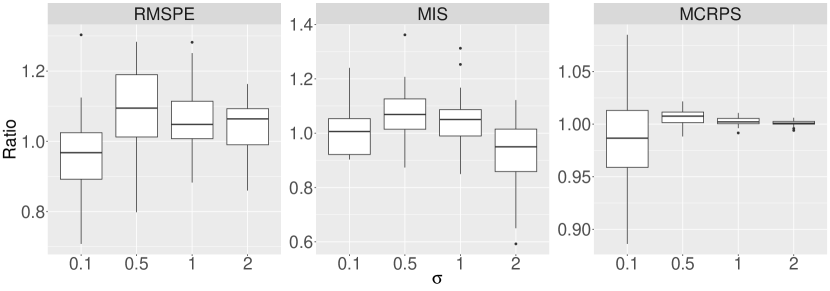
Figure 2: The boxplots of FBART to S-FBART ratios of RMSPEs, MISs and MCRPSs under different noise levels.

Last, we examine the performance of FBART under a variety of noise levels and tuning parameter selections. Specifically, we consider the true regression map in Case 2, with noise level $\sigma\in\{0.1,0.5,1,2\}$, the degree of B-spline basis $q\in\{2,3,4\}$, the number of trees $K\in\{10,20,50\}$, and the number of basis functions $J\in\{5,10,15\}$. Fig. 3 shows the average RMSPEs of FBART based on $10$ simulation runs. As expected, the resulting RMSPE scales approximately linearly with $\sigma$. In addition, we observe that choosing a larger $K$ can improve the prediction accuracy, and empirically using $K=10$ trees is sufficient to deliver comparable prediction results to those of using larger numbers of trees. With respect to the dimension $J$ of the basis functions, we find that a moderately large dimension ($J=10$) is adequate. In Section S.2.2 of the Supplementary Materials, it is shown that the MCRPS results of FBART are also quite robust to different specifications of tuning parameters.

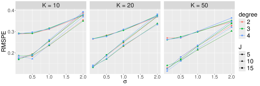
Figure 3: The performance of FBART under different tuning parameter specifications.

6 Real Data Illustrations

The proposed FBART and S-FBART methods are applied to two real datasets, each exhibiting a specific shape constraint on the response curves. For comparison, we also provide prediction results for BART and mBART as described in Section 5; note that the latter is only considered when the response curves appear to be monotonic. The BFOSR and LLR methods are not considered here because the real datasets contain curves observed at different sampling points, and their available implementations are not applicable to this case. The performance of all methods is evaluated using RMSPE, mean absolute prediction error (MAPE) and MCRPS on the test sets; the mean negatively oriented interval score (MIS) criterion is not considered here, since the true regression map is unknown for real datasets. Implementation details and additional results are given in Section S.3 of the Supplementary Materials.

6.1 Data Description

Given the significant concern of energy challenges in modern society, accurate prediction of battery performance is crucial for battery production and optimization. The first dataset, Battery, contains capacity values of $124$ lithium-ion batteries cycled under fast-charging conditions (Severson et al., 2019). Our target is to predict the battery’s capacity fade curve, where battery capacity is treated as a function of the number of charge-discharge cycles. Following Severson et al. (2019), the prediction starts from cycle $101$ onward, with $p=9$ features constructed from the early-cycle data (the data in the cycles from $1$ to $100$) as the covariates. We randomly select $93$ curves for training, with the remaining $31$ curves for testing. A Logit transformation is performed on the capacity values to make the Gaussian noise assumption more applicable. For the capacity fade curves, it is reasonable to assume that they are monotonically decreasing in cycle numbers (see Figure S.9 in the Supplementary Materials).

Economists have long been interested in studying the impact of various variables on individual incomes (e.g., Card, 1999; Rubinstein and Weiss, 2006). The second dataset, Wage, contains weekly wages of full-time working males in the United States in 1987 (see the data object ex2019 in the R package Sleuth2; Ramsey and Schafer, 2002). Our focus here is to explore the relationship between the wage curve (wages versus work experience) and workers’ features, including years of education, whether the person is black, whether the workplace is in a city, and the region of the person’s workplace (i.e., $p=4$). We randomly select $n=15,000$ samples for training and the remaining $10,437$ samples for testing. The prior studies (e.g., Hannah and Dunson, 2013; Chernina and Gimpelson, 2023) have suggested that it is reasonable to assume that wages exhibit a concave relationship with the years of experience variable (see Figure S.11 in the Supplementary Materials).

For FBART and S-FBART, we choose $J=10$, $q=4$, and $K=10$. In the case of S-FBART, a monotonically decreasing constraint is introduced for the Battery dataset, while a concavity constraint is applied to the Wage dataset. For BART and mBART, the numbers of trees are selected by a four-fold cross-validation.

6.2 Results

Table 2: The prediction results of different methods on the Battery and Wage datasets.

	Battery				Wage
Method	RMSPE	MAPE	MCRPS	Decreasing	RMSPE	MAPE	MCRPS	Concave
FBART	$0.039$	$0.022$	$0.163$	✗	369.049	235.364	180.355	✗
S-FBART	0.034	0.019	0.134	✓	$369.952$	$236.763$	$180.966$	✓
BART	$0.043$	$0.025$	$0.297$	✗	$371.970$	$239.588$	$181.410$	✗
mBART	$0.039$	$0.025$	$0.255$	✓	-	-	-	-

The prediction results of the two real datasets are summarized in Table 2, with the best results highlighted in bold font. We also include a “Decreasing” column for Battery and a “Concave” column for Wage to indicate whether a method accounts for the shape information of the response curves. We observe that for both datasets, the proposed FBART and S-FBART models consistently outperform the competing methods in terms of prediction accuracy and probabilistic prediction. This demonstrates the benefits of accounting for responses’ functional nature. Notably, S-FBART offers flexibility in incorporating various shape constraints, whereas mBART is limited to modeling monotone curves. When comparing S-FBART with FBART, we find that S-FBART is superior to FBART in terms of the three evaluation criteria for the Battery dataset, while delivering slightly inferior results than those of FBART on the Wage dataset. The advantage of FBART over S-FBART is likely due to the high noise level present in the Wage dataset, an evidence supported by our simulation results.

7 Conclusion

We have proposed a highly flexible Bayesian approach for the function-on-scalar regression (FOSR) problem with potential shape constraints on the response curves. To the best of our knowledge, FBART is the first Bayesian tree-based method for the FOSR problem, and S-FBART is the first theoretically backed-up Bayesian nonparametric approach for the shape-constrained FOSR. The proposed methods are especially preferred when dealing with a highly nonlinear regression map defined on a complex covariate space.

Our proposed methods can be extended in several ways. In this paper, we have assumed independent noises. To incorporate within-curve covariance structure, we may model $\{\epsilon_{ij}\}$ using a Gaussian process with a parametric covariance function. This can be implemented with a minor modification of Algorithm 1, where variance-covariance parameters could be sampled via an extra Metropolis-Hastings step. Another potential extension is to consider multivariate functional data. This could be achieved by introducing a multivariable B-spline basis via tensor product, or by constructing an additive model where each term depends on one or two variables. Lastly, we note that S-FBART could potentially be used for the quantile-on-scalar or distribution-on-scalar regression problems, since quantile functions are non-decreasing functions that are closely related to the $2$-Wasserstein space.

References

- Abraham and Khadraoui (2015) Abraham, C. and K. Khadraoui (2015). Bayesian regression with b-splines under combinations of shape constraints and smoothness properties. Statistica Neerlandica 69(2), 150–170.
- Birke and Dette (2007) Birke, M. and H. Dette (2007). Estimating a convex function in nonparametric regression. Scandinavian Journal of Statistics 34(2), 384–404.
- Botev (2017) Botev, Z. I. (2017). The normal law under linear restrictions: simulation and estimation via minimax tilting. Journal of the Royal Statistical Society Series B: Statistical Methodology 79(1), 125–148.
- Card (1999) Card, D. (1999). The causal effect of education on earnings. Handbook of labor economics 3, 1801–1863.
- Chen et al. (2016) Chen, Y., J. Goldsmith, and R. T. Ogden (2016). Variable selection in function-on-scalar regression. Stat 5(1), 88–101.
- Chernina and Gimpelson (2023) Chernina, E. and V. Gimpelson (2023). Do wages grow with experience? deciphering the russian puzzle. Journal of Comparative Economics 51(2), 545–563.
- Chiou et al. (2004) Chiou, J.-M., H.-G. Müller, and J.-L. Wang (2004). Functional response models. Statistica Sinica 14, 675–693.
- Chipman et al. (1998) Chipman, H. A., E. I. George, and R. E. McCulloch (1998). Bayesian cart model search. Journal of the American Statistical Association 93(443), 935–948.
- Chipman et al. (2010) Chipman, H. A., E. I. George, and R. E. McCulloch (2010). BART: Bayesian additive regression trees. The Annals of Applied Statistics 4(1), 266 – 298.
- Chipman et al. (2022) Chipman, H. A., E. I. George, R. E. McCulloch, and T. S. Shively (2022). mbart: multidimensional monotone bart. Bayesian Analysis 17(2), 515–544.
- de Boor (1978) de Boor, C. (1978). A Practical Guide to Splines (1 ed.). Applied Mathematical Sciences. Springer New York, NY. Published: 29 November 2001.
- De Boor and Daniel (1974) De Boor, C. and J. W. Daniel (1974). Splines with nonnegative B-spline coefficients. Mathematics of Computation 28(126), 565–568.
- Denison et al. (1998) Denison, D. G., B. K. Mallick, and A. F. Smith (1998). A bayesian cart algorithm. Biometrika 85(2), 363–377.
- Fan and Müller (2022) Fan, J. and H.-G. Müller (2022). Conditional distribution regression for functional responses. Scandinavian Journal of Statistics 49(2), 502–524.
- Ge et al. (2019) Ge, S., S. Wang, Y. W. Teh, L. Wang, and L. Elliott (2019). Random tessellation forests. Advances in Neural Information Processing Systems 32.
- Genz and Bretz (2009) Genz, A. and F. Bretz (2009). Computation of multivariate normal and t probabilities, Volume 195. Springer Science & Business Media.
- Ghosal et al. (2023) Ghosal, R., S. Ghosh, J. Urbanek, J. A. Schrack, and V. Zipunnikov (2023). Shape-constrained estimation in functional regression with bernstein polynomials. Computational Statistics & Data Analysis 178, 107614.
- Ghosal and van der Vaart (2007) Ghosal, S. and A. van der Vaart (2007). Convergence rates of posterior distributions for noniid observations. Annals of Statistics 35(1), 192–223.
- Ghosal and Van der Vaart (2017) Ghosal, S. and A. Van der Vaart (2017). Fundamentals of Nonparametric Bayesian Inference, Volume 44. Cambridge University Press.
- Gneiting and Raftery (2007) Gneiting, T. and A. E. Raftery (2007). Strictly proper scoring rules, prediction, and estimation. Journal of the American Statistical Association 102(477), 359–378.
- Greven and Scheipl (2017) Greven, S. and F. Scheipl (2017). A general framework for functional regression modelling. Statistical Modelling 17(1-2), 1–35.
- Groeneboom and Jongbloed (2014) Groeneboom, P. and G. Jongbloed (2014). Nonparametric estimation under shape constraints. Number 38. Cambridge University Press.
- Hannah and Dunson (2013) Hannah, L. A. and D. B. Dunson (2013). Multivariate convex regression with adaptive partitioning. The Journal of Machine Learning Research 14(1), 3261–3294.
- Hill et al. (2020) Hill, J., A. Linero, and J. Murray (2020). Bayesian additive regression trees: A review and look forward. Annual Review of Statistics and Its Application 7, 251–278.
- Horowitz and Lee (2017) Horowitz, J. L. and S. Lee (2017). Nonparametric estimation and inference under shape restrictions. Journal of Econometrics 201(1), 108–126.
- Kapelner and Bleich (2016) Kapelner, A. and J. Bleich (2016). bartmachine: Machine learning with bayesian additive regression trees. Journal of Statistical Software 70, 1–40.
- Kotecha and Djuric (1999) Kotecha, J. H. and P. M. Djuric (1999). Gibbs sampling approach for generation of truncated multivariate gaussian random variables. In 1999 IEEE international conference on acoustics, speech, and signal processing. Proceedings. ICASSP99 (Cat. No. 99CH36258), Volume 3, pp. 1757–1760. IEEE.
- Kowal and Bourgeois (2020) Kowal, D. R. and D. C. Bourgeois (2020). Bayesian function-on-scalars regression for high-dimensional data. Journal of Computational and Graphical Statistics 29(3), 629–638.
- Li et al. (2023) Li, Y., A. R. Linero, and J. Murray (2023). Adaptive conditional distribution estimation with bayesian decision tree ensembles. Journal of the American Statistical Association 118(543), 2129–2142.
- Linero (2018) Linero, A. R. (2018). Bayesian regression trees for high-dimensional prediction and variable selection. Journal of the American Statistical Association 113(522), 626–636.
- Linero and Yang (2018) Linero, A. R. and Y. Yang (2018). Bayesian regression tree ensembles that adapt to smoothness and sparsity. Journal of the Royal Statistical Society Series B: Statistical Methodology 80(5), 1087–1110.
- Liu et al. (2021) Liu, Y., V. Ročková, and Y. Wang (2021). Variable selection with abc bayesian forests. Journal of the Royal Statistical Society Series B: Statistical Methodology 83(3), 453–481.
- Luo et al. (2021) Luo, Z. T., H. Sang, and B. Mallick (2021). Bast: Bayesian additive regression spanning trees for complex constrained domain. Advances in Neural Information Processing Systems 34, 90–102.
- Martínez-Hernández and Genton (2020) Martínez-Hernández, I. and M. G. Genton (2020). Recent developments in complex and spatially correlated functional data. Brazilian Journal of Probability and Statistics 34, 204–229.
- Morris (2015) Morris, J. S. (2015). Functional regression. Annual Review of Statistics and Its Application 2, 321–359.
- Morris and Carroll (2006) Morris, J. S. and R. J. Carroll (2006). Wavelet-based functional mixed models. Journal of the Royal Statistical Society Series B: Statistical Methodology 68(2), 179–199.
- Müller (2005) Müller, H.-G. (2005). Functional modelling and classification of longitudinal data. Scandinavian Journal of Statistics 32, 223–240.
- Petersen and Müller (2019) Petersen, A. and H.-G. Müller (2019). Fréchet regression for random objects with euclidean predictors. The Annals of Statistics 47(2), 691–719.
- Pya and Wood (2015) Pya, N. and S. N. Wood (2015). Shape constrained additive models. Statistics and computing 25, 543–559.
- Ramsay and Dalzell (1991) Ramsay, J. and C. Dalzell (1991). Some tools for functional data analysis. Journal of the Royal Statistical Society: Series B (Methodological) 53(3), 539–561.
- Ramsay and Silverman (2005) Ramsay, J. O. and B. W. Silverman (2005). Functional Data Analysis (2 ed.). Springer Series in Statistics. Springer New York, NY. Published: 08 June 2005, Softcover Published: 10 November 2010, eBook Published: 28 June 2006.
- Ramsey and Schafer (2002) Ramsey, F. L. and D. W. Schafer (2002). The Statistical Sleuth: A Course in Methods of Data Analysis (2nd ed.). Duxbury/Thomson Learning.
- Ray and Mallick (2006) Ray, S. and B. Mallick (2006). Functional clustering by Bayesian wavelet methods. Journal of the Royal Statistical Society: Series B (Statistical Methodology) 68, 305–332.
- Ročková and Saha (2019) Ročková, V. and E. Saha (2019). On theory for bart. In The 22nd international conference on artificial intelligence and statistics, pp. 2839–2848. PMLR.
- Ročková and Van der Pas (2020) Ročková, V. and S. Van der Pas (2020). Posterior concentration for bayesian regression trees and forests. The Annals of Statistics 48(4), 2108–2131.
- Rosen and Thompson (2009) Rosen, O. and W. K. Thompson (2009). A bayesian regression model for multivariate functional data. Computational statistics & data analysis 53(11), 3773–3786.
- Rubinstein and Weiss (2006) Rubinstein, Y. and Y. Weiss (2006). Post schooling wage growth: Investment, search and learning. Handbook of the Economics of Education 1, 1–67.
- Scheipl et al. (2015) Scheipl, F., A.-M. Staicu, and S. Greven (2015). Functional additive mixed models. Journal of Computational and Graphical Statistics 24(2), 477–501.
- Severson et al. (2019) Severson, K. A., P. M. Attia, N. Jin, N. Perkins, B. Jiang, Z. Yang, M. H. Chen, M. Aykol, P. K. Herring, D. Fraggedakis, et al. (2019). Data-driven prediction of battery cycle life before capacity degradation. Nature Energy 4(5), 383–391.
- Tang and Müller (2008) Tang, R. and H.-G. Müller (2008). Pairwise curve synchronization for functional data. Biometrika 95, 875–889.
- Um et al. (2023) Um, S., A. R. Linero, D. Sinha, and D. Bandyopadhyay (2023). Bayesian additive regression trees for multivariate skewed responses. Statistics in Medicine 42(3), 246–263.
- Unser et al. (1993) Unser, M., A. Aldroubi, and M. Eden (1993). B-spline signal processing. ii. efficiency design and applications. IEEE transactions on signal processing 41(2), 834–848.
- Wang et al. (2016) Wang, J.-L., J.-M. Chiou, and H.-G. Müller (2016). Functional data analysis. Annual Review of Statistics and its application 3, 257–295.
- Wang and Yan (2021) Wang, W. and J. Yan (2021). Shape-restricted regression splines with r package splines2. Journal of Data Science 19(3), 498–517.
- Yang et al. (2020) Yang, H., V. Baladandayuthapani, A. U. Rao, and J. S. Morris (2020). Quantile function on scalar regression analysis for distributional data. Journal of the American Statistical Association 115(529), 90–106.
- Yao et al. (2005) Yao, F., H.-G. Müller, and J.-L. Wang (2005). Functional linear regression analysis for longitudinal data. Annals of statistics 33(6), 2873–2903.
- Zhang et al. (2022) Zhang, Z., X. Wang, L. Kong, and H. Zhu (2022). High-dimensional spatial quantile function-on-scalar regression. Journal of the American Statistical Association 117(539), 1563–1578.