Minimum Copula Divergence for Robust Estimation
Abstract
This paper introduces a robust estimation framework based solely on the copula function. We begin by introducing a family of divergence measures tailored for copulas, including the -, -, and -copula divergences, which quantify the discrepancy between a parametric copula model and an empirical copula derived from data independently of marginal specifications. Using these divergence measures, we propose the minimum copula divergence estimator (MCDE), an estimation method that minimizes the divergence between the model and the empirical copula. The framework proves particularly effective in addressing model misspecifications and analyzing heavy-tailed data, where traditional methods such as the maximum likelihood estimator (MLE) may fail. Theoretical results show that common copula families, including Archimedean and elliptical copulas, satisfy conditions ensuring the boundedness of divergence-based estimators, thereby guaranteeing the robustness of MCDE, especially in the presence of extreme observations. Numerical examples further underscore MCDE’s ability to adapt to varying dependence structures, ensuring its utility in real-world scenarios.
keywords: Divergence, Long tail, Influence function, Model misspecification
1 Introduction
Copulas are mathematical functions that capture the dependence structure between random variables, allowing for the construction of multivariate distributions by combining univariate marginal distributions with a copula that describes their interdependencies. This separation is particularly useful in modeling complex relationships where variables exhibit nonlinear or asymmetric dependencies.
In finance, copulas are extensively used to model and manage risks associated with multiple financial assets. They enable the assessment of joint default probabilities in credit risk management, the pricing of complex derivatives like collateralized debt obligations, and the evaluation of portfolio risk by capturing tail dependencies that traditional correlation measures might miss. For instance, copulas have been applied to monitor market risk in basket products and to measure credit risk in large pools of loans, cf. McNeil et al., (2015); Patton, (2006). In engineering, copulas facilitate the analysis of systems where component dependencies significantly impact overall reliability. They have been applied in structural engineering to assess the reliability of tower and tower-line systems under varying loads, such as wind or earthquakes. In environmental sciences, copulas are employed to model and analyze dependencies between various environmental factors. For example, they have been used to study the joint distribution of temperature and precipitation in the Mediterranean region, providing insights into climate patterns. See, for example, Bevilacqua et al., (2024) for an application to spatial copula modeling.
Despite these successful applications, several challenges remain. Traditional estimation methods such as the maximum likelihood estimator (MLE) often prove highly sensitive to model misspecifications and extreme observations, particularly in high-dimensional settings or when data exhibit heavy tails. In many cases, the accuracy of copula-based models is compromised by the need to correctly specify marginal distributions, which can be difficult in practice and may lead to biased dependence estimates. These issues underscore the need for robust methodologies that can isolate and accurately capture the underlying dependence structure even under adverse conditions. Our proposed framework, based on copula divergence, can directly address these challenges by bypassing marginal assumptions and mitigating the influence of outliers, thereby enhancing the reliability of dependence modeling across diverse fields.
For this, we introduce a family of divergence functionals defined on the space of copula functions, called copula divergence. Specifically, as variants of copula divergence, the -copula, -copula, and -copula divergences are presented, where the parameters , and represent the respective power exponents characterizing each divergence. For a parametric copula model, the estimator is proposed by minimization for the copula divergence between the model copula and the empirical copula with respect to the parameter, which is called the minimum copula divergence estimator (MCDE). In this way, MCDE is a rank statistic as a functional of the empirical copula function like Kendall’s and Spearman’s , and it differs fundamentally from the MLE. Thus, MCDE can exhibit greater robustness to extreme observations, while the log-likelihood (even the pseudo-likelihood) can be more sensitive if the copula density blows up near corners or edges. MLE is often asymptotically efficient if the model is correctly specified (it achieves the Cramér-Rao bound). However, it can suffer from large bias or variance in smaller samples, especially under heavy tails. MCDE might lose a bit of asymptotic efficiency relative to MLE in the perfect-model scenario, but can be more robust under misspecification or contamination. In computational aspects, MLE, for many copula families, requires evaluating and differentiating the copula density. Some integrals or boundary terms can complicate the process, especially in higher dimensions. MCDE typically only needs to evaluate values of the copula model function, and an associated divergence functional. For many Archimedean or elliptical copulas, the model function is simpler to handle without requiring partial derivatives than the corresponding density function.
The rest of this paper is organized as follows. Section 2 discusses common copula models and the power-boundedness. Section 3 formalizes the MCDE and its properties. Section 4 explores influence functions and robustness. Section 5 provides examples of Archimedean copula.
2 Copula models
Let us consider statistical inference about copula functions. Copulas are functions that describe the dependence structure between random variables. They separate the joint distribution of random variables into two parts: the marginal distributions of each random variable and the copula function capturing dependence. Sklar’s theorem states that for a vector of random variables with joint distribution and marginals , there exists a copula such that
In particular, for continuous marginals, is unique. See Nelsen, (2006) for a comprehensive introduction. We consider a copula model
where is an unknown parameter of a parameter space that is an open subset of . See Joe, (2014) for detailed treatment of copulas to model complex dependence structures.
2.1 Common copula models
We highlight two important families of copula models: Archimedean copulas and elliptical copulas.
Archimedean Copulas: They form a widely used class characterized by a generator function , see Genest and Rivest, (1993). They are often appealing due to their analytic simplicity and ability to model both tail dependence and asymmetry (depending on the generator). An Archimedean copula in dimensions is defined by
where is a continuous, strictly decreasing generator function with , and is the (generalized) inverse function of . Crucially, to ensure the required properties. Many well-known one-parameter Archimedean copulas can be written in terms of their generator .
-
•
Clayton Copula:
-
•
Gumbel Copula:
-
•
Frank Copula:
-
•
Joe Copula:
Elliptical Copulas
Elliptical distributions induce to copula functions arisen from such as the multivariate normal (Gaussian) or multivariate -distribution. They are useful for modeling symmetric dependence structures.
-
•
Gaussian Copula: Derived from the multivariate normal distribution, the Gaussian copula is defined using the standard normal cumulative distribution function (CDF) and the multivariate normal CDF (with mean and correlation matrix ):
Here, is the standard normal quantile function.
-
•
Student- Copula: Arising from the multivariate -distribution, the Student- copula uses the univariate -distribution CDF (with degrees of freedom) and its multivariate counterpart :
Its heavier tails facilitate modeling of data that exhibit stronger tail dependence.
2.2 Power-bounded copula model
We introduce a plausible assumption regarding the lower tail behavior of copula models. For simplicity, we suppose a bivariate copula model , and the discussion will be easily extended to multivariate cases. We say a copula model is power-bounded if satisfies
| (1) |
for any , where denotes a gradient vector for . Usually, may blow up near , where . See Charpentier and Segers, (2009) for related discussion for copula behaviors near the corners of the unit square. The condition (1) indicates that multiplying by effectively controls the potential blow-up of the log-derivative near the boundaries. In fact, this power-boundedness condition is satisfied for many popular Archimedean copula families. Table 1 summarizes the supremum values of these powered log-derivatives for several typical copula functions. Although the derivations in Appendix A involve intricate calculus, the essential idea is straightforward: one can show that
near . This bounded behavior is also clearly illustrated in Figure 1, which displays the log-derivative function for the specific case .
| Clayton | |||
|---|---|---|---|
| Gumbel | |||
| Frank | |||
| Joe |

We next consider a Gaussian copula model that is defined as:
where is a bivariate standard normal cumulative distribution function with correlation parameter , and is the inverse of the univariate standard normal cumulative distribution function. Then, as , the following limits hold:
The proof is given in Appendix B. We remark that diverging property for the log-derivative of the Gaussian copula comes from the exponential decay of the Gaussian distribution in the left tail. On the other hand, the Student t-copula function has only a polynomial decay. Hence, becomes bounded.
Building on these models and their properties, the remainder of this work investigates divergence-based methods for estimating copula parameters. In particular, we explore how divergences can yield robust and efficient procedures for a variety of copula families, including both Archimedean and elliptical. For this we introduce copula divergence, typically the power copula divergence and its variants.
3 Copula divergence
We introduce a family of copula-based divergences. This differs from standard density-based divergences like the Kullback-Leibler divergence and other density divergences. See Csiszár, (1967); Basu et al., (1998); Jones et al., (2001); Fujisawa and Eguchi, (2008); Eguchi and Komori, (2022) for many variants of density divergence. In principle, copula divergences focus exclusively on the dependence structure among variables, while density divergences measure discrepancies in the entire joint distribution–including both dependence and marginals. Copula divergences remove the influence of marginal distributions and directly quantify how the shape of the dependence structures differs. This can be more robust when the margins are unknown or contaminated, and it directly addresses questions such as “How does the association (e.g., tail dependence) differ between two copulas?”
Let be the set of all the copula functions defined on a hypercube . A functional defined on is called a divergence if satisfies
with equality if and only if for almost all of . Let us discuss three types of power divergence as follows.
-
•
-copula divergence:
-
•
-copula divergence:
-
•
-copula divergence:
Here ‘’ in the above equations represents integration with respect to the measure induced by . For the -copula divergence, if , then it reduces to the Hellinger squared distance
| (2) |
If , then it reduces to the extended KL-divergence
Let be a strictly convex function defined on with and . Then, -divergence is defined by
If we choose as
then the -divergence is nothing but the -copula divergence. See Csiszár, (1967) for the case of density divergence.
For the -copula divergence, if , it reduces to the Cramér-von-Mises divergence
| (3) |
If , it reduces to the extended KL-divergence . If , it reduces to the Itakura-Saito divergence
Moreover, the -copula divergence has a natural extension from the power function to a convex function as a generator function. Let be a strictly increasing and convex function defined on . Then, -divergence is defined by
where is the inverse of the derivative function of . It is noted that with equality if and only if since from the assumption of . If , then , so that the -divergence is reduced to the -power divergence.
For the -copula divergence, if ,
This is associated with the Cauchy-Schwartz inequality. See Fujisawa and Eguchi, (2008); Eguchi et al., (2011); Eguchi, (2024) for the -density divergence and the geometric perspectives.
We remark that, if is taken a limit to , then the -copula diagonal entropy is written as
This is nothing but the geometric mean of , say . Thus,
which is called the geometric-mean divergence. For , then the -copula diagonal entropy is a half of the harmonic mean of :
and hence the harmonic mean divergence is given by
In general, copula divergences focus only on differences in dependence structures. Their derivation is often numerically simpler for many copula models, since they require evaluating the copula function rather than integrating the copula density function. Naturally, we expect that copula divergences are robust to marginal misspecification, since they measure the dependence structure on pseudo-observations. In this work, we explore the estimation methods based on copula divergences.
3.1 Minimum copula divergence
We apply copula divergences to estimate a parameter in a copula model . Copula divergences are specifically designed to measure how two dependence structures differ, irrespective of marginal changes discussed in the preceding section. Hence, the advantageous property can be transferred to such copula-based estimators. Let us give a mathematical formulation for proposed estimators.
For a random sample , the pseudo vector is defined by
| (4) |
and the empirical copula function is defined by
| (5) |
where represents the indicator function. Let be a copula divergence. Thus, the minimum copula divergence estimator (MCDE) for is defined by
| (6) |
The empirical copula converges weakly to a mean-zero Gaussian process:
where is a general Gaussian process with the mean and covariance given by
where denotes the coordinatewise minimum . See Segers, (2012) for rigorous discussion and wide perspectives. Hence the limit is a kind of multivariate Brownian bridge governed by the true copula , one might call it a copula-based Brownian sheet.
We define a functional
Under regularity conditions (identifiability, interior solution, differentiability of , etc.), it can be applied to the functional delta method for at noting . By the continuous mapping theorem, since in probability in , see Segers, (2012); Vaart and Wellner, (2023); Billingsley, (2013). Moreover, weakly converges to a normal distribution with mean and covariance . The covariance matrix is derived by the sandwich formula as a typical example for the M-estimator. The concrete form will be given for specific examples of copula divergence . We will use a learning algorithm to find the numerical minimizer for a MCDE. Routinely, a stochastic gradient algorithm is suggested as
The computational complexity is usually reasonable rather than that for the MLE accompanied by the evaluation of the copula density functions as discussed later.
One advantage of MCDE is that, when defining divergences purely in terms of copulas (rather than their densities), one avoids complicated integrals. The construction of the empirical copula bypasses the need to integrate or differentiate a parametric copula density, benefiting numerical stability and computational efficiency, especially in high-dimensional settings. It is worthwhile to emphasize how the pseudo-observations come from the empirical distribution of each margin, making MCDE a purely rank-based approach. Thus, MCDE has an advantage such that any scaling or monotonic transformations of the original data do not affect the estimated copula parameter. The present proposal is closely related to the copula divergence discussed in De Keyser and Gijbels, (2024), which relies on the copula density functions. It can be referred to as the kernel-based divergence to estimate copulas, see Alquier et al., (2023) for statistical performance.
By working with directly, the estimation has a semiparametric flavor: the marginals are replaced by their empirical distributions , and only the dependence structure is modeled parametrically. We focus on the loss function defined by a copula divergence , i.e., . Typically, there are loss functions by three type of copula divergences as follows:
-
•
-power loss:
and is called -MCDE, where are observed pseudo vectors defined in (4). The -estimating equation is given by , where
(7) -
•
-power loss:
and is called -MCDE. The -estimating equation is given by , where
(8) -
•
-power loss:
and is called -MCDE. The estimating equation is given by , where
(9) Here
The -estimating function (7) consists of three multiplicative factors: gives a weight to each observation according to the model’s own predicted copula value; is the difference between the model value and the empirical value in the power sense; gives the direction or the gradient for the estimating function. When is small, there is less penalty imposed in regions where is very small, which can yield a degree of robustness near the boundary . When is larger, the function places more importance on getting the model’s values correct even in small-copula regions, potentially improving efficiency under ideal conditions but also becoming more sensitive to boundary outliers. Similarly, the -loss function is associated with the -divergence:
up to the constant. The estimating equation is given by
On the other hand, the -estimating equation is a linear functional of the empirical copula function and is decomposed into three factors similar to -estimating equation. In particular, can be negative to give more weight to points where the copula value is small and less weight otherwise. This can sometimes be beneficial if one wants to place emphasis on tail regions. Similarly, the -loss function is given by
and the estimating function is given by
The -estimating function (9) is the same as -copula estimating function (8) except for the extra weight if the power exponents and match. The extra weight is the ratio of the cross and diagonal entropy, , in which it provides an additional global scale adaptation noting when . See Fujisawa and Eguchi, (2008) for detailed discussion of the super robustness as density divergence.
We explore the asymptotic distributions of three types of power MCDEs under a correctly specified model.
Proposition 1.
Assume that is the empirical copula defined in (5) generated from a copula model . Let , , and be the -MCDE, the -MCDE, and the -MCDE, respectively. Then,
-
. ,
-
. ,
-
. .
Here, for , where
| (10) | ||||
| (11) | ||||
Proof.
By the definition of -MCDE ,
The Taylor theorem yields
Hence multiplying both sides by yields
We observe that
and hence
By the continuous mapping theorem,
which is equal to a normal distribution with mean and covariance , where is defined in (11) with . This is because the empirical copula converges weakly to a mean-zero Gaussian process:
where is a general Gaussian process with the mean and covariance given by
where . We observe, as
in probability, which is equal to in (10). In accordance with these, noting
An argument for the -MCDE similar to that for the -MCDE yields
noting
in probability. Hence, . Similarly, for the -MCDE,
since coverges to in probability. This concludes . The proof is complete. ∎
The proof is based on the standard discussion for deriving the asymptotics of M-estimators such as the sandwich formula and Slutsky’s theorem. We note the asymptotic distribution for the -MCDE does not depend on . This is closely related with such a property that the minimum -density divergent estimator has a unique asymptotic distribution independent of , see Eguchi, (1983). As for the -MCDE, when , the asymptotic variance equals that of the -MCDE. When the power exponents and equal, then the asymptotic variance for the -MCDE equals that of the -MCDE. This is because the extra weight converges to in probability.
3.2 Robust minimum copula divergence
We discuss how the class of MCDEs can be framed and compared with both the MLE and minimum density divergence estimators. We focus on the methodological motivations, theoretical implications, and practical ways to strengthen the argument in favor of MCDE. The copula-based approach, justified by Sklar’s theorem, naturally separates a joint distribution into marginal distributions and a copula capturing dependence. The MCDE is appealing because it focuses solely on the copula component-marginal distributions (and their densities) need not be explicitly specified or estimated. In contrast, density-based approaches such as the MLE or minimum density divergence estimators often involve specifying or approximating the full joint density . For clarifying this, we give a foundational assumption for the copula model, which could correspond to that for the density model such as exponential family. The key idea is to allow sufficiently flexible behaviors for of the copula functions in the tail.
As introduced in the preceding section, we have discussed a few forms of power copula divergences with power exponents , , and and the asymptotic distributions under a correctly specified model. Each choice yields a different copula-based loss function and estimating equation. This unifies common metrics (e.g., Hellinger, Kullback–Leibler, Itakura–Saito) under a single umbrella and provides a range of options for balancing robustness and efficiency. An important aspect of choosing a suitable divergence is controlling the estimator’s sensitivity to outliers, particularly in the tails. Let us investigate statistical properties for MCDEs: All three estimating functions for -, -, and -MCDEs have the following properties:
Proposition 2.
Proof.
By the definition (7),
If , then
due to . This implies is uniformly bounded in from the assumption of the power-boundedness for . Similarly, for ,
This implies the uniform boundedness for from the assumption. Finally, for ,
since . This implies the uniform boundedness for from the assumption. ∎
This implies the influence functions of the three MCDEs with are all bounded, and hence their MCDEs are led to be qualitatively robust. To compare the usual estimators including the maximum likelihood estimator we will have numerical experiments in several settings of simulated data generations. The behaviors of MCDEs should be investigated in the presence of misspecification, in particular, outliers in the upper or lower tail.
By selecting different , , or parameters, one can tune how the estimator reacts to misspecification or extreme observations. Here is a natural question about which value of the power exponent is optimal? For this, we discuss a data-driven selection of the exponent by cross-validation for a practical situation, where it is not known whether the underlying distribution follows a correctly specified model, or a misspecified model. Consider a selection for the optimal value of to get good estimator in the family of -MCDEs. Let , and is randomly divided into folds:
Each fold contains approximately samples. We use as the training set and use as the validation set recursively in in the -fold cross validation. Let , where is in a grid set of candidates, say . Here
where is the empirical copula based on . Finally, for the empirical copula is based on we evaluate as a predictor for by the Cramér-von-Mises divergence defined in (3). Note is a fixed -copula divergence with . In this way, we define the optimal as
It is worthwhile to note that and are statistically independent by construction of ’s. The optimal can escape from over-leaning thanks to the partition of and . A simple numerical experiment will be given in a subsequent discussion.
We discuss the characteristics for MCDEs to compare the usual estimators under a copula model. Typically, the MLE is defined on the model of probability density functions induced from the copula model: The density function of is given by
where ’s are the cumulative distribution functions (CDFs) with the probability density functions ’s, and
| (12) |
In this way, the negative log-likelihood function can be written as if the CDF ’s are known. In effect, there are a few variants of MLEs depending on the way to estimate for marginal CDFs. The approach to imposes parametric forms on both margins and the copula is guaranteed to be more efficient if everything is correctly specified. However, it is more susceptible to misspecification errors in either the margins or copula leading to bias, especially in heavy-tailed scenarios.
We focus on the semiparametric MLE defined by minimization of
where ’s are pseudo observation vectors defined in (4). This approach ignores direct parametric assumptions on the margins. Instead, it uses empirical distribution functions to transform to . It is more flexible than fully parametric MLE because we do not impose parametric forms on each marginal distribution. The estimation function is given by
The semiparametric MLEs are widely used for estimating the parameter for the asymptotic efficiency with a technically complicated correction, however, it has a weak point for the robustness. This is because the function is often unbounded in in common copula models. For example, consider the Clayton copula model, in which the density function is given by
This implies
up to a constant. Hence, we observe as since the log-derivative can involve terms such as , , , and so on.
Alternatively, density-based divergences can capture full differences between two distributions encompassing both marginals and dependence. Even if one needs to focus only on dependence, then a density divergence can be a comprehensive choice–but often at the expense of more complexity and potentially less robustness if the marginals are uncertain. For example, the -copula loss functions for a parametric copula density function can be considered as
| (13) |
It can provide a robust estimation, however, the multiple integral in the second term has no closed form even for common copula models. For this, there needs numerical integration procedures like MCMC sampling each step in the learning algorithm to find the minimum of the loss function in . Furthermore, a condition of the robustness for this estimator is suggested in more complicated than that for the MCDE as given in a subsequent discussion. In this way, we will explore further aspects for MCDE rather than the minimum density divergence estimator.
With MCDE, the parametric copula distribution function is required rather than its density . Numerically, this is often much simpler since we only need to evaluate at pseudo-observations, without having to differentiate or integrate the copula function over . The MLE for copulas often comes from assuming both marginal distributions and a parametric form for the dependence structure, or from a pseudo-likelihood approach if marginals are nonparametric. This can be quite sensitive to tail misspecification. Under correct specification, the MLE may be asymptotically efficient. However, it can fail badly under heavy tails or outlier contamination. Divergence-based estimators (particularly those that are robust) may exhibit smaller bias or variance under model misspecification, at the cost of a small efficiency loss in the ideal case.
4 Numerical experiments
Let us have small-scale numerical experiments. Consider a Clayton copula model:
| (14) |
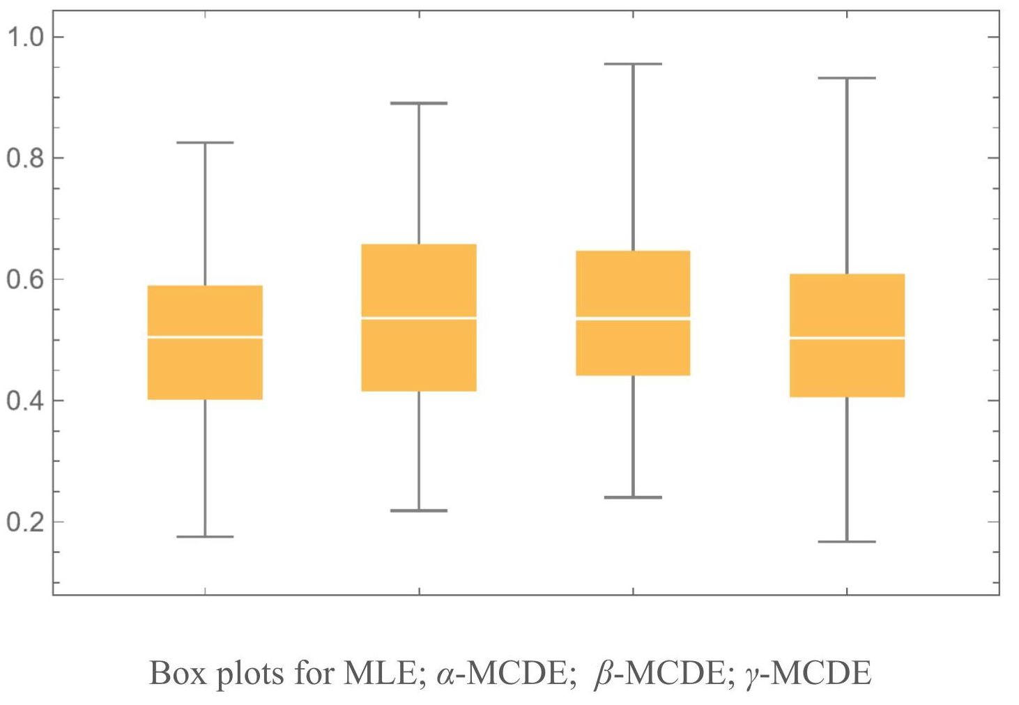
for . First, data is generated from the correctly specified Clayton copula model with observations, where is set as . Thus, we find four estimators: the semiparametric MLE, -MCDE (), -MCDE () and -MCDE (). The result of the numerical evaluation for these estimators with repetitions is given in Table 2 and Figure 2. The semiparametric MLE has the best performance among four estimators in the sense of the root mean squared error (RMSE), in which three MCDEs are almost equivalent performance. The tendency can be observed for other choice for these power exponents , , and .
| Mean | RMSE | |
|---|---|---|
| MLE | 0.5016 | 0.1410 |
| -MCDE | 0.5311 | 0.1514 |
| -MCDE | 0.5424 | 0.1679 |
| -MCDE | 0.5043 | 0.1654 |
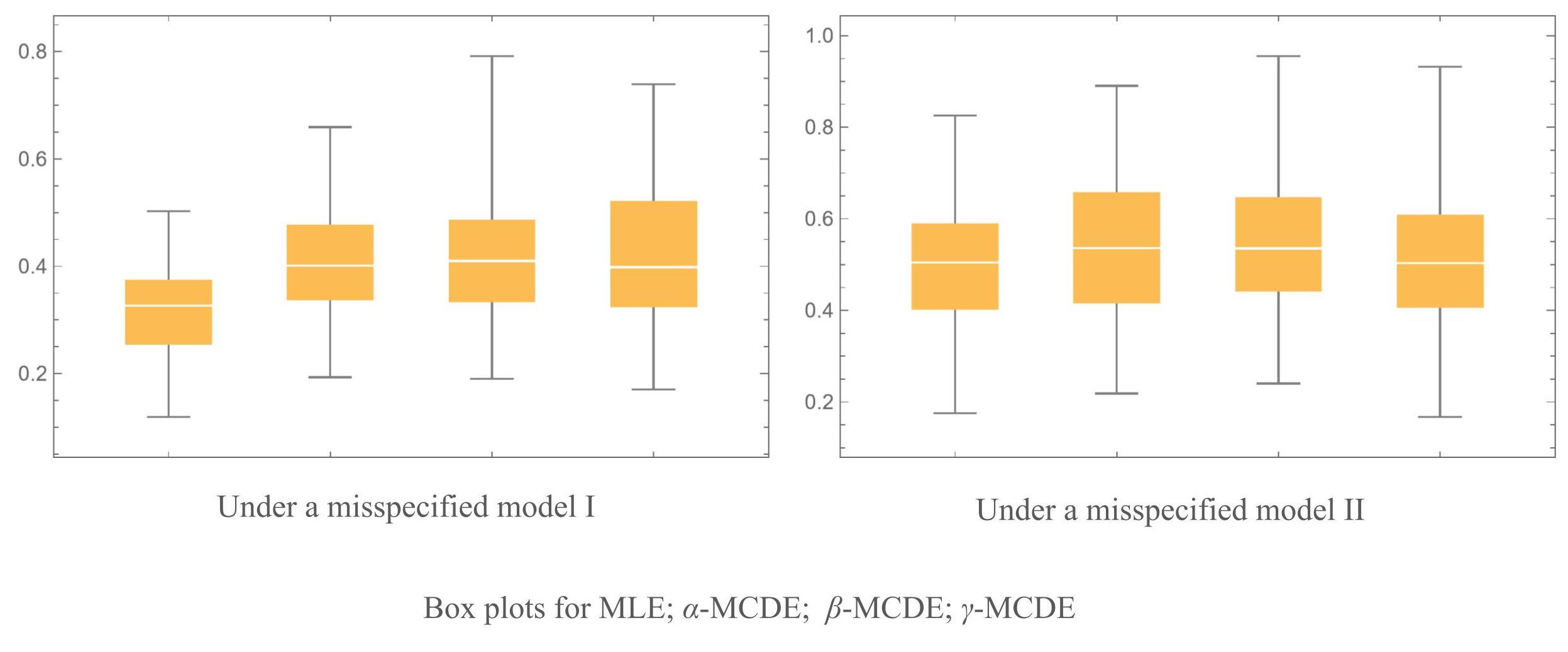
Secondly, we now consider a type I of the model misspecified as
| (15) |
where is set as and is a Student t-copula function with correlation and degrees of freedom. Data is generated from the misspecified model with observations with the true . The result of the numerical evaluation for these estimators with repetitions is given in Table 3 and Figure 3. Under the misspecified model, the semiparametric MLE still tries to fit a single Clayton copula to data that partly come from a Student t-copula. Consequently, its estimate of is pulled away from the nominal truth . This results in a bias (e.g., in Table 2, the MLE mean is 0.1652 vs. the true 0.5 and a larger RMSE of 0.3467. In contrast, the robust estimators -, -, and -MCDEs downweight (in different ways) outliers or small subsets of data that do not follow the assumed model. As a result, these estimators exhibit: Smaller bias relative to MLE and significantly smaller RMSE. We next consider a type II of misspecification with a distribution
where is set as and is a bivariate normal distribution function with mean and covariance . This setting introduces another type of misspecification in the marginal distributions, causing the MLE to collapse: its mean estimate is 0.3167, distant from the true 0.5, and the RMSE increases to 0.2065. By contrast, all variants of the MCDE estimators remain stable against this severe misspecification, and their performance remains comparable to that under the correctly specified model (see Table 3).
| Misspecified case I | Misspecified case II | |||
|---|---|---|---|---|
| Mean | RMSE | Mean | RMSE | |
| MLE | 0.1652 | 0.3467 | 0.3167 | 0.2065 |
| -MCDE | 0.2722 | 0.2471 | 0.4122 | 0.1397 |
| -MCDE | 0.2629 | 0.2592 | 0.4199 | 0.1621 |
| -MCDE | 0.2993 | 0.2297 | 0.4200 | 0.1593 |
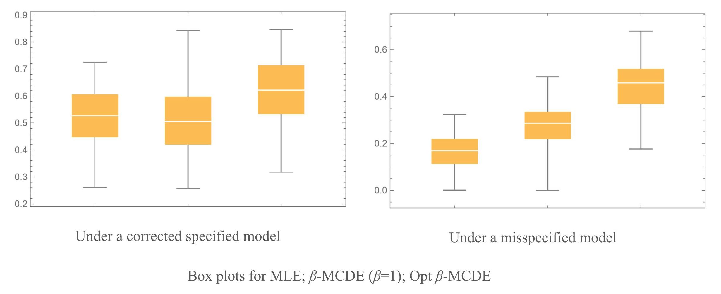
Next, we investigate a numerical performance for the data-driven selection for the exponent discussed in the preceding section. For this, we conduct a five-fold cross validation to get cross-validated errors. Similarly, we consider the corrupted copula (15) for the Clayton model with a heavy contamination such as and degrees of freedom for the Student t-copula. Thus, comparison among MLE, the -MCDE fixed as and the optimal -MCDE was conducted with repetitions : The outputs are given in Table 4 and Figure 4 for the correctly specified model and the misspecified model. The semiparametric MLE and the fixed -MCDE perform better than the optimal -MCED in the correctly specified model, in which the optimal -MCED has a bit worse performance compared to the fixed -MCDE due to the effect of the selection for . On the other hand, the MLE performs the worst in the misspecified model, and the data-driven “optimal” -MCDE has better performance than the fixed -MCDE.
| Correctly specified case | Misspecified case | |||
|---|---|---|---|---|
| Mean | RMSE | Mean | RMSE | |
| MLE | 0.5280 | 0.1084 | 0.1571 | 0.3510 |
| -MCDE | 0.5118 | 0.1261 | 0.2722 | 0.2519 |
| Opt -MCDE | 0.6207 | 0.1687 | 0.3378 | 0.1866 |
Finally, to illustrate the practical relevance of our methods, we apply them to a real-world bivariate dataset consisting of 251 daily log-returns for Microsoft and Apple during 2024, using data obtained from Google Finance, (2024). This smaller-scale sample provides a concrete setting in which to evaluate how the proposed estimators handle the pronounced tail risk often found in financial returns. The conditional lower tail (CLT) probability is defined as
where is the pseudo vector derived from the log-return data and is the empirical probability measure.
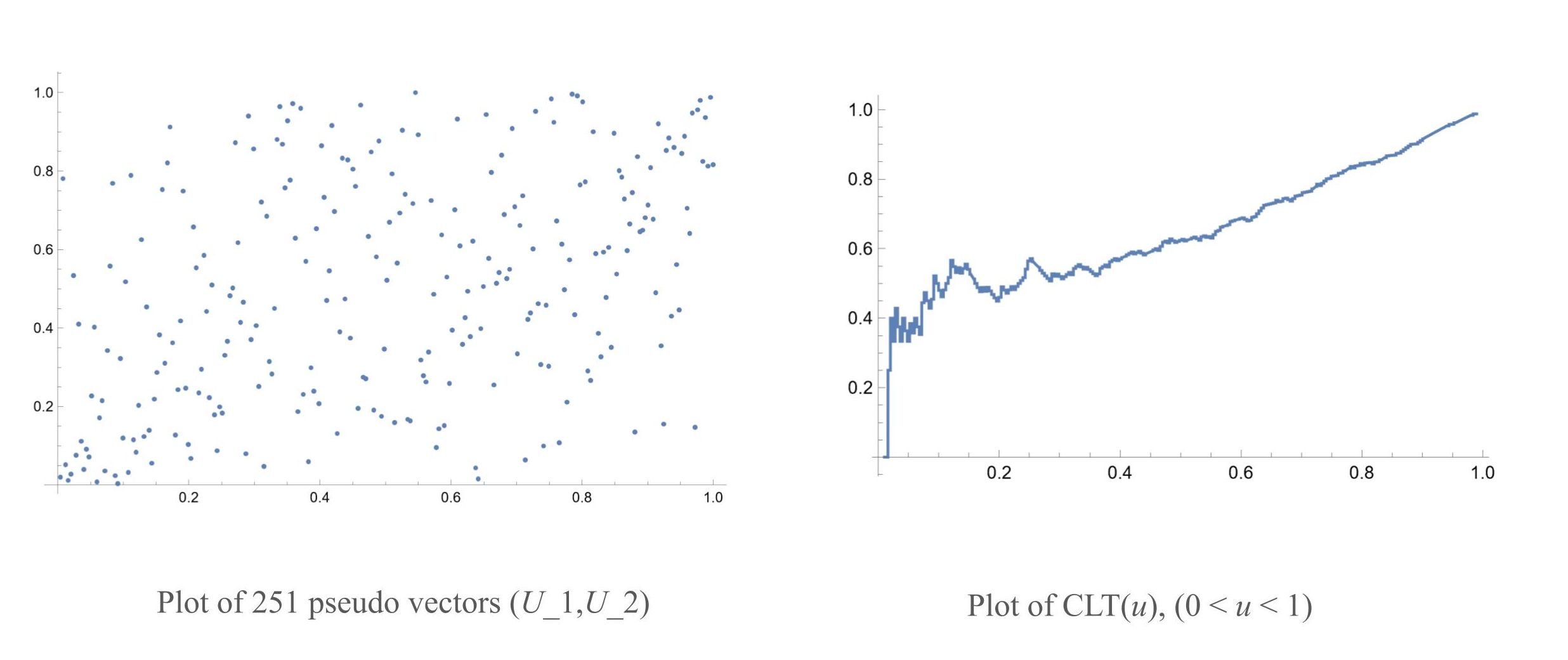
There is a heavy lower tail dependence as seen in Figure 5. Hence, we adopt the Clayton copula model (14) with a parameter , and four estimators suggested reasonable values between 0.70 and 0.85 in Table 5
| no. of outliers | MLE | -MCDE | -MCDE | -MCDE |
|---|---|---|---|---|
| 0 | 0.7687 | 0.8063 | 0.8401 | 0.7195 |
| 10 | 0.4188 | 0.5406 | 0.5774 | 0.5217 |
| 20 | 0.1768 | 0.3689 | 0.3853 | 0.3611 |
| 30 | 0.0296 | 0.2464 | 0.2390 | 0.2373 |
| 35 | 0.0060 | 0.1967 | 0.1760 | 0.1829 |
Let us examine the influence adding to the outliers generated from a bivariate normal distribution with mean and covariance . Here
are the sample mean and covariance of the daily log-returns, respectively. In this way, we adopt the normal distribution with artificially a shifted mean to act as an outlier-generating distribution in the analysis. This large mean shift ensures that any samples drawn from this distribution will appear as ‘extreme’ points (outliers) relative to the main data. This leads to outliers that lie in opposite directions (e.g., large with small ).
Table 5 clearly shows how the semiparametric MLE estimate collapses as even modest numbers of outliers are introduced, whereas the various MCDE-based estimators degrade much more gracefully. This is a compelling demonstration of the practical robustness properties of MCDE: With zero noise, all estimators are fairly close, lying between 0.71 and 0.84; As outliers increase, MLE suddenly falls down from 0.77 down to 0.01, while the MCDE variants still yield plausible (though smaller) estimates, reflecting their reduced sensitivity to contamination. From a methodological standpoint, these results illustrate that heavy-tailed financial data combined with outliers or data contamination can severely bias the classical likelihood-based estimate. In contrast, robust estimators such as -MCDE, -MCDE, and -MCDE can retain stability in tail-dependence estimation. This discrepancy might underscore the importance of adopting robust estimation procedures in risk, however, it needs a more comprehensive examination across different time spans and under additional parametric copula models in tail analysis. In summary, these results illustrate that if tail outliers are plausible in financial data (especially in daily returns where market jumps occur), then robust estimation methods can be quite valuable.
5 Concluding remarks
This paper introduces and develops the concept of minimum copula divergence as a robust estimation framework for analyzing dependence structures among variables. By isolating the copula component from marginal distributions, the proposed method effectively addresses challenges posed by non-linear or asymmetric relationships. This approach is not only theoretically sound but also highly versatile, as demonstrated through its potential applications in diverse fields such as finance, machine learning, and ecology.
One of the primary contributions of this study is the formulation of a robust estimator that is resilient to outliers and model misspecifications. Theoretical results, coupled with numerical experiments, underscore the superiority of MCDE over conventional estimation methods under various contamination scenarios. The use of divergence-based metrics provides a flexible and robust alternative for modeling dependence structures, particularly in high-dimensional or noisy data environments.
An additional advantage of the MCDE framework lies in its nonparametric nature, which leverages rank statistics to estimate dependence structures. By relying on rank-based measures, MCDE avoids assumptions about specific parametric forms of the marginal distributions, thereby enhancing its robustness and generalizability. This nonparametric property also makes MCDE particularly suitable for datasets where parametric assumptions are difficult to justify or validate. The implications of MCDE extend beyond its immediate statistical applications. Its ability to model intricate dependency patterns opens doors for innovations in areas where understanding complex relationships is critical. For example, in financial risk management, MCDE can improve portfolio optimization by accurately capturing tail dependencies. Similarly, in ecological studies, it can facilitate more reliable predictions of species distributions under uncertain conditions.
MCDE’s relationship with optimal transport theory presents another intriguing avenue for exploration. Optimal transport, a framework rooted in information geometry, provides a powerful tool for analyzing the geometry of probability distributions. See Amari and Nagaoka, (2000); Eguchi, (1983, 1992); Eguchi and Copas, (2006) for extensive discussion and statistical applications. By aligning the objectives of MCDE with those of optimal transport, such as minimizing divergence in the distributional sense, future work could further enhance the theoretical foundation of robust dependency modeling. The coupling of MCDE with concepts from information geometry could yield deeper insights into the structure of dependence and improve its adaptability to complex, real-world data scenarios.
Despite its strengths, the framework is not without limitations. The computational complexity of estimating divergence measures in high-dimensional settings warrants further optimization. Moreover, the choice of divergence function and its impact on estimator performance require additional investigation. Addressing these issues will enhance the practical applicability of MCDE. Future research directions include exploring alternative divergence measures and extending the methodology to dynamic or time-varying copula models. Additionally, integrating MCDE with machine learning techniques could provide novel insights and improve predictive capabilities in data-intensive applications.
In conclusion, this study establishes MCDE as a promising tool for robust estimation in dependency modeling. By bridging theoretical advancements and practical applications, it lays the groundwork for future innovations in robust statistical methods and their interdisciplinary applications.
Appendix A Power-boundedness for common copulas
A.1 Clayton copula
By definition,
and hence the partial derivative with respect to :
We then consider the limit as . By setting , we simplify the expression:
and
Thus, the expression becomes:
| (16) |
where . As , for , so the LHS in (16) tends to 0. Considering different paths, such as , we find that the limit is consistent across different paths and tends to 0. This simplifies to analyzing the behavior in a neighborhood of (0,0) along a particular path. Therefore, the limit is:
A.2 Gumbel copula
By definition,
Hence,
where . By setting , we simplify the expression:
and
Therefore, the limit expression of is:
as , , and the exponential term decays to 0 for , while the polynomial and logarithmic terms grow slower than the exponential decay. For , the expression simplifies to:
which tends to infinity as . Therefore, the limit is:
A.3 Frank copula
Since
we approximate for small and :
This implies
Now, we observe
for small and . Therefore,
A.4 Joe copula function
Since
we approximate for small and :
Therefore,
now, consider the product :
as , for , and remains 1 for . In summary,
Appendix B Power-boundedness for Gaussian copula
The Gaussian copula can be written as where . For large negative , is very small, a standard Laplace-type asymptotic for the bivariate normal CDF shows that
up to polynomial factors in , where
Then, for , Thus, we obtain:
which is unbounded in absolute value as . Therefore,
and hence
Noting from the previous asymptotic,
Therefore the product remains dominated by an exponentially decaying factor for any , while the derivative factor grows only polynomially. Hence
References
- Alquier et al., (2023) Alquier, P., Chérief-Abdellatif, B.-E., Derumigny, A., and Fermanian, J.-D. (2023). Estimation of copulas via maximum mean discrepancy. Journal of the American Statistical Association, 118(543):1997–2012.
- Amari and Nagaoka, (2000) Amari, S.-i. and Nagaoka, H. (2000). Methods of information geometry, volume 191. American Mathematical Soc.
- Basu et al., (1998) Basu, A., Harris, I. R., Hjort, N. L., and Jones, M. C. (1998). Robust and efficient estimation by minimising a density power divergence. Biometrika, 85(3):549–559.
- Bevilacqua et al., (2024) Bevilacqua, M., Alvarado, E., and Caamaño-Carrillo, C. (2024). A flexible clayton-like spatial copula with application to bounded support data. Journal of Multivariate Analysis, 201:105277.
- Billingsley, (2013) Billingsley, P. (2013). Convergence of probability measures. John Wiley & Sons.
- Charpentier and Segers, (2009) Charpentier, A. and Segers, J. (2009). Tails of multivariate archimedean copulas. Journal of Multivariate Analysis, 100(7):1521–1537.
- Csiszár, (1967) Csiszár, I. (1967). On information-type measure of difference of probability distributions and indirect observations. Studia Sci. Math. Hungar., 2:299–318.
- De Keyser and Gijbels, (2024) De Keyser, S. and Gijbels, I. (2024). Parametric dependence between random vectors via copula-based divergence measures. Journal of Multivariate Analysis, 203:105336.
- Eguchi, (1983) Eguchi, S. (1983). Second order efficiency of minimum contrast estimators in a curved exponential family. The Annals of Statistics, pages 793–803.
- Eguchi, (1992) Eguchi, S. (1992). Geometry of minimum contrast. Hiroshima Mathematical Journal, 22(3):631–647.
- Eguchi, (2024) Eguchi, S. (2024). Minimum gamma divergence for regression and classification problems. arXiv preprint arXiv:2408.01893.
- Eguchi and Copas, (2006) Eguchi, S. and Copas, J. (2006). Interpreting kullback–leibler divergence with the neyman–pearson lemma. Journal of Multivariate Analysis, 97(9):2034–2040.
- Eguchi and Komori, (2022) Eguchi, S. and Komori, O. (2022). Minimum Divergence Methods in Statistical Machine Learning: From an Information Geometric Viewpoint. Springer, Tokyo.
- Eguchi et al., (2011) Eguchi, S., Komori, O., and Kato, S. (2011). Projective power entropy and maximum tsallis entropy distributions. Entropy, 13(10):1746–1764.
- Fujisawa and Eguchi, (2008) Fujisawa, H. and Eguchi, S. (2008). Robust parameter estimation with a small bias against heavy contamination. J. Multivar. Anal., 99(9):2053–2081.
- Genest and Rivest, (1993) Genest, C. and Rivest, L.-P. (1993). Statistical inference procedures for bivariate archimedean copulas. Journal of the American statistical Association, 88(423):1034–1043.
- Google Finance, (2024) Google Finance (2024). Historical price data for microsoft (msft) and apple (aapl). Accessed January 20, 2025.
- Joe, (2014) Joe, H. (2014). Dependence modeling with copulas. CRC press.
- Jones et al., (2001) Jones, M., Hjort, N. L., Harris, I. R., and Basu, A. (2001). A comparison of related density-based minimum divergence estimators. Biometrika, pages 865–873.
- McNeil et al., (2015) McNeil, A. J., Frey, R., and Embrechts, P. (2015). Quantitative risk management: concepts, techniques and tools-revised edition. Princeton university press.
- Nelsen, (2006) Nelsen, R. B. (2006). An introduction to copulas. Springer.
- Patton, (2006) Patton, A. J. (2006). Modelling asymmetric exchange rate dependence. International economic review, 47(2):527–556.
- Segers, (2012) Segers, J. (2012). Asymptotics of empirical copula processes under non-restrictive smoothness assumptions. Bernoulli, 18(3):764–782.
- Vaart and Wellner, (2023) Vaart, A. v. d. and Wellner, J. A. (2023). Empirical processes. In Weak Convergence and Empirical Processes: With Applications to Statistics, pages 127–384. Springer.