Effect of thermal conduction on accretion shocks in relativistic magnetized flows around rotating black holes

Abstract

We examine the effects of thermal conduction on relativistic, magnetized, viscous, advective accretion flows around rotating black holes considering bremsstrahlung and synchrotron cooling processes. Assuming the toroidal component of magnetic fields as the dominant one, we self-consistently solve the steady-state fluid equations to derive the global transonic accretion solutions for a black hole of spin $a_{\rm k}$. Depending on the model parameters, the magnetized accretion flow undergoes shock transitions and shock-induced global accretion solutions persist over a wide range of model parameters including the conduction parameter ($\Upsilon_{\rm s}$), plasma-$\beta$, and viscosity parameter ($\alpha_{\rm B}$). We find that the shock properties—such as shock radius ($r_{\rm s}$), compression ratio ($R$), and shock strength ($S$)—are regulated by $\Upsilon_{\rm s}$, plasma $\beta$, and $\alpha_{\rm B}$. Furthermore, we compute the critical conduction parameter ($\Upsilon_{\rm s}^{\rm cri}$), a threshold beyond which shock formation ceases to exist, and investigate its dependence on plasma-$\beta$ and $\alpha_{\rm B}$ for both weakly rotating ($a_{\rm k}\rightarrow 0$) and rapidly rotating ($a_{\rm k}\rightarrow 1$) black holes. Finally, we examine the spectral energy distribution (SED) of the accretion disc and observe that increased thermal conduction and magnetic field strength lead to more luminous emission spectra from black hole sources.

I Introduction

Black holes are believed to be the central to some of the most energetic phenomena in the universe, such as active galactic nuclei (AGNs) and X-ray binaries (XRBs) (Remillard and McClintock, 2006; Netzer, 2013, and references therein). The accretion process plays a key role in driving black hole dynamics, offering essential insights into the observational signatures of these enigmatic objects. Recent groundbreaking images of Sgr A^∗ Event Horizon Telescope Collaboration et al. (2022) and M87 Event Horizon Telescope Collaboration et al. (2021) have revealed these supermassive black holes are surrounded by a hot, magnetized plasma. These AGNs are generally powered by advection-dominated accretion flows Narayan and Yi (1994, 1995); Yuan and Narayan (2014), which exhibit a low-density profile that results in their characteristic low luminosity Ho (2008); Netzer (2013). This behavior is due to the inability of low-density plasma to cool efficiently through radiation, leading to flow temperatures that approach the virial temperature. Such high temperature and low density accretion flows are well-suited to explain the observational features of accreting super massive black hole systems Yuan and Narayan (2014). Moreover, ubiquitous magnetic fields in accreting system plays pivotal role in describing the structure of the accretion flow as well Oda et al. (2007); Sarkar and Das (2016); Das and Sarkar (2018); Jana and Das (2024).

In the hot, low density plasma of magnetized advective accretion flows, where the particle mean free path are significantly long, thermal conduction emerges as a crucial mechanism for energy transport. Hence, Thus, thermal conduction exerts a significant influence on the structure,and thermodynamic properties of hot accretion flows. Meanwhile, Tanaka and Menou (2006) estimated the mean free path using Chandra Observatory data from Sgr A* and proposed that accretion in this system occurs under weakly collisional conditions. In such regimes, the mean free path exceeds the characteristic length scale of the system, such as the gravitational radius ($r_{g}$). They also suggested that thermal conduction plays a pivotal role in driving the formation of outflows and winds. Furthermore, Johnson and Quataert (2007) and Sharma et al. (2008) carried out comprehensive studies on the influence of electron thermal conduction in spherical hot accretion flows. Afterwards, numerous efforts were made using self-similar approach to emphasize the significant role of thermal conduction in shaping the behavior of black hole accretion systems in presence of bipolar outflows Tanaka and Menou (2006); Shadmehri (2008); Faghei (2012); Khajenabi and Shadmehri (2013); Ghoreyshi and Shadmehri (2020). Recently, Mitra et al. (2023) studied the global accretion solutions and showed that the inclusion of thermal conduction notably modifies their transonic characteristics.

Accretion flow around black hole is inherently transonic as subsonic flow from the outer edge of the accretion disc eventually crosses the black hole horizon at supersonic speed. Such smooth transition happens at the critical points ($r_{\rm c}$). As the accretion progresses, rotating supersonic flow experiences centrifugal repulsion and flow is decelerated causing matter to accumulate in the vicinity of the black hole. When this accumulation exceeds a critical threshold, centrifugal barrier triggers a shock transition, provided Rankine-Hugoniot shock conditions are satisfied Landau and Lifshitz (1959). The second law of thermodynamics further favors the formation of shock in a magnetized viscous advective accretion flows around black hole that naturally drives the accreting mater toward the state of higher entropy Becker and Kazanas (2001); Mitra and Das (2024). The phenomenon of shock formation in accretion around black holes has been extensively studied by various group of researchers, both theoretically and numerically considering hydrodynamics as well as magnetohydrodynamic scenarios Fukue (1987); Chakrabarti (1989); Chakrabarti and Molteni (1993); Molteni et al. (1994); Yang and Kafatos (1995); Chakrabarti (1996); Molteni et al. (1996); Ryu et al. (1997); Lanzafame et al. (1998); Lu et al. (1999); Das et al. (2001); Becker and Kazanas (2001); Chakrabarti and Das (2004); Le and Becker (2004); Fukumura and Tsuruta (2004); Takahashi et al. (2006); Das (2007); Fukumura et al. (2007); Becker et al. (2008); Das et al. (2009); Kumar et al. (2013); Das et al. (2014); Okuda and Das (2015); Suková and Janiuk (2015); Fukumura et al. (2016); Sarkar and Das (2016); Suková et al. (2017); Aktar et al. (2017); Dihingia et al. (2018, 2019); Kim et al. (2019); Okuda et al. (2019); Dihingia et al. (2020); Sen et al. (2022); Singh and Das (2024a, b); Mitra and Das (2024); Debnath et al. (2024); TianLe-Zhao et al. (2024); Patra et al. (2024); Singh and Das (2024a); Jana and Das (2024). The shock-induced accretion solutions offer a compelling explanation for the spectro-temporal properties commonly observed in black hole candidates Chakrabarti and Titarchuk (1995); Chakrabarti and Manickam (2000); Mandal and Chakrabarti (2005); Nandi et al. (2012); Iyer et al. (2015); Das et al. (2021); Majumder et al. (2022); Nandi et al. (2024). However, the role of thermal conduction in shock-induced, magnetized, viscous, advective accretion flows in presence of radiative cooling processes remains unexplored in the astrophysical literature.

Inspired by this, in the present study, we investigate the structure of a steady, magnetized, viscous, advective accretion flows around rotating black holes incorporating the effects of thermal conduction along with bremsstrahlung and synchrotron cooling mechanisms. We consider that accretion flow is threaded by toroidal magnetic fields surrounding a Kerr black hole, with the gravitational field approximated using the pseudo-potential formulation Dihingia et al. (2018). Moreover, we employ a relativistic equation of state (REoS) that effectively accounts for the thermodynamic variables of the accretion flow. Using this framework, we derive the shock-induced global accretion solutions and investigate key shock properties, such as shock location ($r_{\rm s}$), compression ratio ($R$), and shock strength ($S$), while examining their dependence on thermal conduction and magnetic fields. Finally, we analyze the influence of model parameters on the emission spectrum of supermassive black holes.

The plan of this paper is as follows: In Section II, we outline the basic assumptions, governing equations and solution methodology. Obtained results are presented in Section III. Finally, in Section IV, we summarize our results.

II Governing equations and methodology

We begin with a magnetized, viscous, advective, and axisymmetric low angular momentum accretion flows around a rotating black hole in the presence of thermal conduction. We utilize a cylindrical coordinate system ($r,\phi,z$) and assume that the flow maintains hydrostatic equilibrium in the vertical ($z$) direction. We choose $G=M_{\rm{BH}}=c=1$ to express the flow variables in dimensionless form, where $G$ is the gravitational constant, $M_{\rm{BH}}$ is mass of the black holes, and $c$ is the speed of light. In this unit system, length, angular momentum, and energy are expressed in units of $GM_{\rm{BH}}/c^{2}$, $GM_{\rm{BH}}/c$, and $c^{2}$, respectively. With this, we write the governing equations that describe the motion of the accretion flow around rotating black holes as Dihingia et al. (2018):

$$\upsilon\frac{d\upsilon}{dr}+\frac{1}{h\rho}\frac{dP}{dr}+\frac{d\Psi_{\textrm{e}}^{\textrm{eff}}}{dr}+\frac{\langle B_{\phi}^{2}\rangle}{4\pi r\rho}=0,$$ (1)

$$\dot{M}=2\pi\upsilon\Sigma\sqrt{\Delta},$$ (2)

$$\upsilon\frac{d\lambda}{dr}+\frac{1}{\Sigma r}\frac{d}{dr}(r^{2}T_{r\phi})=0,$$ (3)

$$\frac{\upsilon}{\rho(\Gamma-1)}\left(\frac{dP_{\rm gas}}{dr}-\frac{\Gamma P_{\rm gas}}{\rho}\frac{d\rho}{dr}\right)=\Lambda-\frac{1}{r\rho}\frac{d(rF_{\rm s})}{dr}$$

$$\qquad\qquad\qquad\qquad\qquad\qquad-\alpha_{\rm B}r(P/\rho+\upsilon^{2})\frac{d\Omega}{dr},$$ (4)

$$\frac{\partial\langle B_{\phi}\rangle\hat{\phi}}{\partial t}=\nabla\times\left(\vec{\upsilon}\times\langle B_{\phi}\rangle\hat{\phi}-\frac{4\pi}{c}\eta\vec{j}\right),$$ (5)

where $\upsilon$ is the radial velocity, $\rho$ is the mass density, $h~[=(\epsilon+P_{\rm gas})/\rho]$ is the enthalpy, $B_{\phi}$ denotes the azimuthal component of magnetic fields, and ‘$\langle~\rangle$’ represents the azimuthal average. The total isotropic pressure $P$ is the sum of the gas pressure ($P_{\rm gas}$) and magnetic pressure ($P_{\rm mag}$) with $P_{\rm gas}=R\rho T/\mu$, $R$, $T$ and $\mu$ being the universal gas constant, local flow temperature and mean molecular weight, respectively. In this work, we choose $\mu=0.5$ for fully ionized plasma. Further, we calculate $P_{\rm{mag}}=\frac{\langle B_{\phi}^{2}\rangle}{8\pi}$ and rewrite the total pressure as $P=P_{\rm{gas}}(1+1/\beta)$ where the plasma-$\beta$ parameter is defined as $\beta=P_{\rm{gas}}/P_{\rm{mag}}$. In equation (1), $\Psi_{\rm e}^{\rm eff}$ is the effective potential on the equatorial plane due to a rotating black hole, which is given by Dihingia et al. (2018),

$$\Psi_{\rm e}^{\rm eff}=1+\frac{1}{2}\ln\left[\frac{r\Delta}{a_{\rm k}^{2}(r+2)-4a_{\rm k}\lambda+r^{3}-\lambda^{2}(r-2)}\right],$$ (6)

where $\lambda$ and $a_{\rm k}$ denote the specific angular momentum of the flow and spin of the black hole, respectively, and $\Delta=r^{2}-2r+a_{\rm k}^{2}$.

In equation (2), $\dot{M}$ denotes the mass accretion rate, which remains constant throughout the flow. We express mass accretion rate as ${\dot{m}}={\dot{M}}/{\dot{M}}_{\rm Edd}$, where ${\dot{M}}_{\rm Edd}~(=1.44\times 10^{17}(M_{\rm BH}/M_{\odot})$ gm s${}^{-1})$, $M_{\odot}$ being solar mass. Here, $\Sigma$ refers to the vertically integrated surface mass density of the accreting matter, given by $\Sigma=2\rho H$ Matsumoto et al. (1984), where $H$ is the local half-thickness of the . We calculate $H$ as described in Riffert and Herold (1995); Peitz and Appl (1997) and is given by,

$$H=\sqrt{\frac{Pr^{3}(1-\lambda\Omega)}{\rho}\times\frac{(r^{2}+a_{\rm k}^{2})^{2}-2\Delta a_{\rm k}^{2}}{(r^{2}+a_{\rm k}^{2})^{2}+2\Delta a_{\rm k}^{2}}},$$ (7)

where $\Omega$ is angular velocity of the flow and is given by,

$$\Omega=\frac{2a_{\rm k}+\lambda(r-2)}{a_{\rm k}^{2}(r+2)-2a_{\rm k}\lambda+r^{3}}.$$

In equation (3), we consider the vertically integrated total stress, which is predominantly dominated by the $r\phi$ component of the Maxwell stress $T_{r\phi}$, outweighing the contributions from the other components. For an advective flow with substantial radial velocity, we calculate $T_{r\phi}$ as Machida et al. (2006), $T_{r\phi}=\frac{\langle B_{r}B_{\phi}\rangle}{4\pi}H=-\alpha_{\rm B}(W+\Sigma\upsilon^{2})$, where $W$ is the vertically integrated pressure and $\alpha_{\rm B}$ is a constant that regulates the viscous effect inside the .

In this work, we assume that the flow is cooled through both bremsstrahlung and synchrotron processes. The bremsstrahlung and synchrotron rates (in units of erg cm^-3 s^-1) are given by Shapiro and Teukolsky (1983); Rybicki and Lightman (1986); Wardziński and Zdziarski (2000),

$$Q^{\rm brem}=1.4\times 10^{-27}n_{e}^{2}T_{e}^{1/2}(1+4.4\times 10^{-10}T_{e}),$$

$$Q^{\rm syn}=\frac{16}{3}\frac{n_{e}e^{2}}{c}\left(\frac{eB}{m_{e}c}\right)^{2}\left(\frac{k_{B}T_{e}}{m_{e}c^{2}}\right)^{2},$$

where, $n_{e}$ is electron number density, $T_{e}$ is the electron temperature, $e$ is the electron charge, $m_{e}$ is the electron mass, $k_{B}$ is the Boltzmann constant and $B$ is the magnetic fields. With this, we obtain the dimensionless total cooling rate as $\Lambda=(Q^{\rm brem}+Q^{\rm syn})/\rho~\times~(GM_{\rm BH}/c^{5})$. Following Cowie and McKee (1977); Tanaka and Menou (2006), we estimate the saturated conduction flux as $F_{\rm s}=5\Upsilon_{\rm s}\rho\left(\frac{P_{\rm gas}}{\rho}\right)^{3/2}$, where $\Upsilon_{\rm s}$ is the dimensionless saturated conduction parameter (hereafter conduction parameter) lies in the range $0\leq\Upsilon_{\rm s}<1$. And, $\Gamma$ is the adiabatic index of the accreting gas.

The advection rate of the toroidal magnetic field is described using the induction equation, with its azimuthally averaged form presented in equation 5. Here, $\vec{v}$ denotes the velocity vector, $\eta$ represents the resistivity, and $j$ is current density, respectively Oda et al. (2007). Due to the large scale of the accretion , the Reynolds number is typically high, allowing us to neglect the magnetic diffusion term. Furthermore, we disregard the dynamo term and assume that the azimuthally averaged toroidal magnetic fields approach zero at the surface. As a result, the toroidal magnetic flux rate can be expressed as:

$$\dot{\Phi}=-4\pi\upsilon HB_{0}(r),$$ (8)

where, $B_{0}(r)$ is the azimuthally averaged toroidal magnetic field confined to the disc’s equatorial plane. The magnetic flux $\dot{\Phi}$ is not conserved in the accretion flow and may vary inversely with the radial distance $r$. Following Machida et al. (2006); Oda et al. (2007), we consider $\dot{\Phi}\propto r^{-\zeta}$, where $\zeta$ is a parameter representing the magnetic flux advection rate. Taking all these factors into account, the parametric relation for the magnetic flux rate is:

$$\dot{\Phi}(r,\zeta,\dot{M})=\dot{\Phi}_{\rm{edge}}(\dot{M})\left(\frac{r}{r_{\rm{edge}}}\right)^{-\zeta},$$

where $\Phi_{\rm{edge}}$ is the advection rate of toroidal magnetic flux obtained at the outer edge of the ($r_{\rm{edge}}$). In this work, we consider $\zeta=1$ unless stated otherwise.

The flow equations are closed using the relativistic equation of state (REoS) that relates the internal energy $(\epsilon)$, $P_{\rm{gas}}$ and $\rho$ of the accretion flow. To this end, we adopt the REoS proposed by Chattopadhyay and Ryu (2009), which is given by,

$$\epsilon=\frac{\rho f}{\left(1+\frac{m_{p}}{m_{e}}\right)},$$ (9)

with

$$f=\left[1+\Theta\left(\frac{9\Theta+3}{3\Theta+2}\right)\right]+\left[\frac{m_{p}}{m_{e}}+\Theta\left(\frac{9\Theta m_{e}+3m_{p}}{3\Theta m_{e}+2m_{p}}\right)\right],$$ (10)

where $m_{\rm p}$ is the mass of the ions and $\Theta(=k_{B}T/m_{e}c^{2})$ is the dimensionless temperature. Using the REoS, we have the polytropic index as $N=(1/2)(df/d\Theta)$ and adiabatic index $\Gamma=(1+N)/N$. Subsequently, we define the sound speed as $C_{\rm s}=\sqrt{\Gamma P_{\rm gas}/(\epsilon+P_{\rm gas})}=\sqrt{2\Gamma\,\Theta/(f+2\Theta)}$.

We simplify equations (1)- (5) to obtian the wind equation along with the radial gradients of $\Theta$, $\lambda$ and $\beta$ as

$$\frac{d\upsilon}{dr}=\frac{\mathcal{N}(r,\upsilon,\lambda,\Theta)}{\mathcal{D}(r,\upsilon,\lambda,\Theta)},$$ (11)

$$\frac{d\Theta}{dr}=\Theta_{\textrm{1}}+\Theta_{\textrm{2}}\frac{d\upsilon}{dr},$$ (12)

$$\frac{d\lambda}{dr}=\lambda_{\textrm{1}}+\lambda_{\textrm{2}}\frac{d\upsilon}{dr},$$ (13)

$$\frac{d\beta}{dr}=\beta_{\textrm{1}}+\beta_{\textrm{2}}\frac{d\upsilon}{dr}.$$ (14)

In equations (11, 12, 13, 14), the explicit expressions for the quantities $\mathcal{N}$, $\mathcal{D}$, $\Theta_{1}$, $\Theta_{2}$, $\lambda_{1}$, $\lambda_{2}$, $\beta_{1}$, and $\beta_{2}$ are mathematically extensive. Therefore, we provide them in the Appendix.

In order to obtain the global accretion solutions, we simultaneously solve equations (11, 12, 13, 14) (Das, 2007; Sarkar and Das, 2016; Das and Sarkar, 2018; Singh and Das, 2024a, and references therein). In doing so, we consider mass accretion rate ($\dot{m}$), viscosity parameter ($\alpha_{\rm{B}}$), black hole spin ($a_{\rm k}$), and conduction parameter ($\Upsilon_{\rm s}$) as global parameters, since these quantities remain constant throughout. During accretion, the subsonic flow begins its journey from the outer edge of the ($r_{\rm edge}$) and gradually moves toward the black hole. As it progresses, the flow reaches the critical point ($r_{\rm c}$), where it makes smooth transition to supersonic state before entering the black hole. Due to the inherently transonic nature of black hole accretion, the flow must pass through the critical point ($r_{\rm c}$). Hence, we choose $r_{\rm c}$ as reference radius ($r_{\rm ref}$) and supply angular momentum ($\lambda_{c}$) and plasma-$\beta$ ($\beta_{c}$) at $r_{\rm c}$ as local flow parameters. Employing the model parameters, we carry out the critical point analysis and apply l^′Hôpital’s rule to calculate the radial velocity gradient, which takes the form $(dv/dr)_{\rm c}=0/0$ at $r_{\rm c}$. We then solve $\mathcal{N}(r,\upsilon,\lambda,\Theta)=0$ and $\mathcal{D}(r,\upsilon,\lambda,\Theta)=0$ to find radial velocity ($\upsilon_{c}$) and temperature ($\Theta_{c}$) at $r_{\rm c}$. Subsequently, using these flow variables at $r_{\rm c}$, we integrate equations (11), (12), (13), (14) up to horizon ($r_{\rm h}$) and then to the outer edge of the ($r_{\rm edge}$). Finally, we join these two parts of the solution to obtain the global accretion solution, noting the flow variables at $r_{\rm edge}$ as energy $\mathcal{E}_{\rm edge}$, angular momentum $\lambda_{\rm edge}$, plasma-$\beta_{\rm edge}$, radial velocity $\upsilon_{\rm edge}$, and temperature $\Theta_{\rm edge}$. It is important to note that the same global accretion solution can also be derived using the outer boundary flow variables. In the following sections, we will continue to present our results based on these outer boundary flow variables.

Depending on the model parameters, the flow may exhibit either single or multiple critical points. Critical points located near the horizon ($r_{\rm h}$) are referred to as inner critical points ($r_{\rm{in}}$), while those formed at a large distance are known as outer critical points ($r_{\rm{out}}$). Notably, accretion flows with multiple critical points are of particular interest, as they can undergo shock transitions provided Rankine-Hugoniot shock conditions (RHCs) are satisfied. In reality, rotating accreting matter experiences centrifugal repulsion in the vicinity of the black hole, resulting in an accumulation of matter that forms an effective boundary layer around it. However, this accumulation cannot continue indefinitely, as it leads to the ontinuous transitions in the flow variables, manifesting as shock waves at its threshold. This shock transition is in accordance with the second law of thermodynamics, as it is characterized by a higher entropy state of the accreting matter Becker and Kazanas (2001). Due to shock compression, the density and temperature of the convergent flow sharply increase downstream, just after the shock transition, resulting in a hot and dense post-shock flow (hereafter referred to as the post-shock corona, PSC). As a result, the PSC serves as an ideal location for reprocessing soft photons from the pre-shock flow into high energy X-ray radiation through the inverse Comptonization process. These high energy X-rays are commonly observed from black hole X-ray binary (BH-XRB) sources (Chakrabarti and Titarchuk, 1995; Mandal and Chakrabarti, 2005; Nandi et al., 2012; Iyer et al., 2015; Nandi et al., 2018; Majumder et al., 2022, and references therein).

III Result

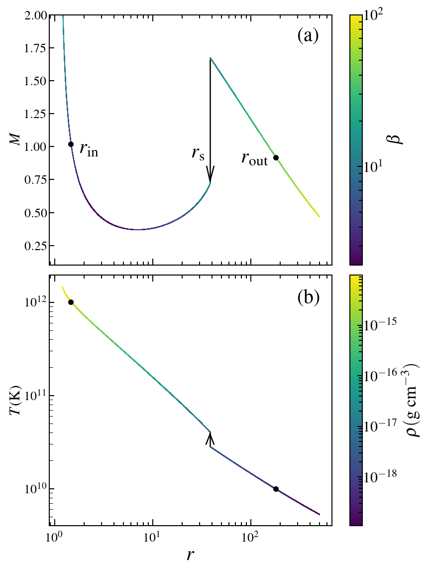
Figure 1: Example of a global shocked-induced accretion solution, where in panel (a) we plot the variation of Mach number ($M=\upsilon/C_{\rm{s}}$) and plasma-$\beta$ (in color) with radial coordinate ($r$), and panel (b) illustrates the temperature ($T$) of the flow along with the density ($\rho$, in color). Here, flow is injected from the outer edge of the $r_{\rm{edge}}=500$ with $\lambda_{\rm{edge}}=2.266$, $\mathcal{E}_{\rm{edge}}=1.00105$, $\beta_{\rm{edge}}=80$, $\alpha_{\rm{B}}=0.01$, $\dot{m}=0.0001$, $\Upsilon_{\rm s}=0.01$, and $a_{\rm{k}}=0.99$. Flow experiences shock transition at $r_{\rm s}=38.37$ indicated by the vertical arrow. Filled circles denote the critical points ($r_{\rm in}$ and $r_{\rm out}$). Color bars in panel (a) and (b) refer the ranges of $\beta$ and $\rho$. See the text for details.

In Fig. 1, we depict an example of a shock-induced global magnetized accretion solution around a rotating black hole in presence of thermal conduction. In panel (a), we show the variation of Mach number ($M=\upsilon/C_{\rm{s}}$) with radius ($r$). Here, we choose $\dot{m}=0.0001$, $\alpha_{\rm{B}}=0.01$ and $\Upsilon_{\rm s}=0.01$, and inject flow subsonically from the outer edge of the at $r_{\rm{edge}}=500$, with angular momentum $\lambda_{\rm{edge}}=2.266$, energy $\mathcal{E}_{\rm{edge}}=1.00105$, plasma-$\beta_{\rm{edge}}=80$ on to a super massive black hole of mass $M_{\rm{BH}}=4.3\times 10^{6}\>\mathrm{M}_{\odot}$ and spin $a_{\rm{k}}=0.99$. The flow becomes supersonic after passing the outer critical point at $r_{\rm{out}}=180.28$ with angular momentum $\lambda_{\rm{out}}=2.056$, and continues to accrete toward the horizon. Meanwhile, RHCs become favorable, and the supersonic upstream flow undergoes a shock transition to the subsonic branch at $r_{\rm{s}}=38.37$, indicated by the vertical arrow. In this work, we consider the shock to be thin and non-dissipative Frank et al. (2002). After the shock, the temperature of the downstream flow is increased as the kinetic energy of the upstream flow is converted into thermal energy in the downstream. Furthermore, due to shock compression, the convergent flow becomes compressed, resulting in an increase in density in the downstream flow (PSC). In Fig. 1b, we show the temperature ($T$) profile of the global shocked accretion solution presented in Fig 1a, with density ($\rho$) variation indicated by colors. The range of the flow density is displayed in the color bar on the right side of panel (b). The density compression across the shock front is characterized by the compression ratio, defined as $R=\Sigma_{+}/\Sigma_{-}$, whereas the temperature jump is quantified by the shock strength, which is defined as $S=M_{-}/M_{+}$. For the shocked solution presented in Fig. 1, we obtain $R=1.93$ and $S=2.31$.

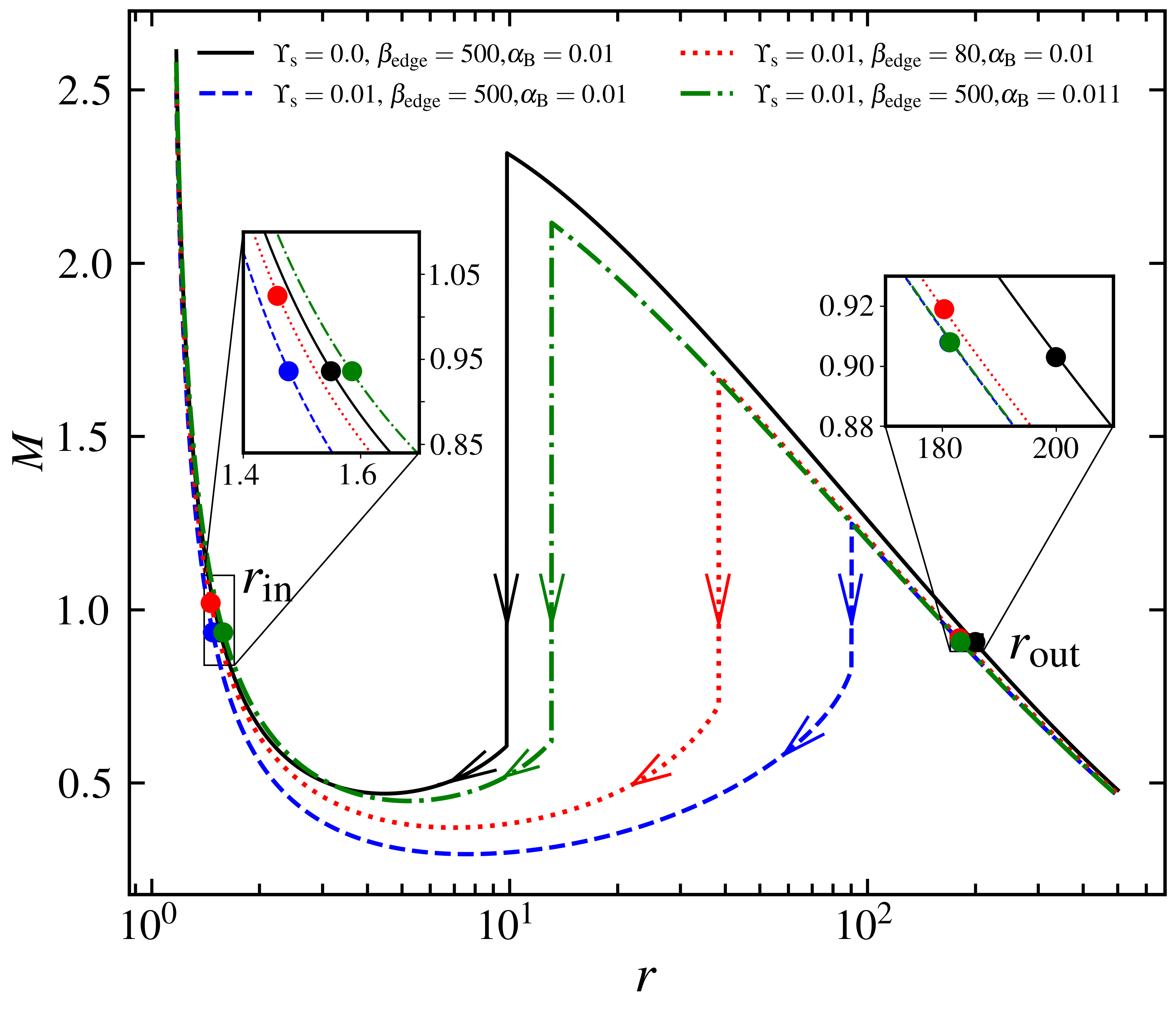
Figure 2: Plot of Mach number $M=\upsilon/C_{\rm s}$ with the radial distance $r$. Flows of fixed $\mathcal{E}_{\rm edge}=1.00105$, $\lambda_{\rm edge}=2.266$ are injected from $r_{\rm{edge}}=500$ with different $\Upsilon_{\rm s}$, $\beta_{\rm edge}$ and $\alpha_{\rm B}$ values. Here, $a_{\rm{k}}=0.99$ and $\dot{m}=0.0001$. Vertical arrows indicate the corresponding shock radii at $r_{\rm s}=9.82$ (solid), $90.24$ (dashed), $38.37$ (dotted) and $13.09$ (dot-dashed). Inner ($r_{\rm in}$) and outer ($r_{\rm out}$) critical points are zoomed at the insets for clarity. See the text for details.

We now investigate the combined influence of viscosity, thermal conduction, and magnetic fields on the shock transition in accretion flows with a fixed outer boundary. In this analysis, we inject matter towards the black hole from the outer edge at $r_{\rm edge}=500$ with a local energy $\mathcal{E}_{\rm edge}=1.00105$ and angular momentum $\lambda_{\rm edge}=2.266$. The mass accretion rate is set to ${\dot{m}}=10^{-4}$, and the Kerr parameter is chosen as $a_{\rm k}=0.99$. For the set of parameters ($\alpha_{\rm B},~\beta_{\rm edge},~\Upsilon_{\rm s})~=~(0.01,~500,~0.0)$, a shock is formed at $r_{\rm s}=9.82$, as indicated by the vertical arrow and the shocked accretion flow solution is shown by the solid (black) curve in Fig. 2. For this solution, we obtain the compression ratio $R=2.74$ and $S=3.81$. The flow passes through both inner and outer critical points at $r_{\rm in}=1.549$ and $r_{\rm out}=199.91$ which are marked using filled circles. When thermal conduction is introduced ($\Upsilon_{\rm s}=0.01$) while keeping the other model parameters fixed, the shock front moves outward to $r_{\rm s}=90.24$. This happens because thermal conduction enhances the local thermal pressure, which in turn pushes the shock to settle at a larger radius Singh and Das (2024b). For this case, we find the inner and outer critical points at $r_{\rm in}=1.477$, and $r_{\rm out}=188.25$, and $(R,~S)~=~(1.39,1.50)$, with the resulting solution represented by the dashed (blue) curve. As the magnetic field strength is increased to $\beta_{\rm edge}=80$ with $\Upsilon_{\rm s}=0.01$ and $\alpha_{\rm B}=0.01$, we observe that the shock front moves toward the horizon as indicated by the dotted red vertical arrow at $r_{\rm s}=38.37$. Here, the inner and outer critical points are at $r_{\rm in}=1.458$, and $r_{\rm out}=180.28$, and $(R,~S)~=~(1.93,2.31)$. This inward movement of the shock is expected, as the density and temperature in the post-shock region (PSC) are higher than in the upstream flow. This results in more intense cooling, which reduces the thermal pressure, ultimately causing the shock to move inward. Overall, it is evident that thermal conduction induces effect opposite to the magnetic fields in determining the shock transitions. Finally, when viscosity is increased ($\alpha_{\rm B}=0.011$), while maintaining $\Upsilon_{\rm s}=0.01$ and $\beta_{\rm edge}=500$, we observe that the shock moves further inward to $r_{\rm s}=13.09$, as indicated by the dot-dashed (green) vertical arrow. The increased viscosity facilitates more efficient angular momentum transport, weakening the centrifugal repulsion and causing the shock to move inward. For this solution, we find the inner and outer critical points at $r_{\rm in}=1.582$, and $r_{\rm out}=180.36$, and $(R,~S)~=~(2.55,3.40)$. We tabulate the model parameters and shock properties in Table 1. With these findings, we point out that the combined effects of thermal conduction, viscosity, and magnetic fields regulate the shock properties, including the size of the post-shock corona ($r_{\rm s}$), density compression ($R$) and temperature jump ($S$).

Table 1: Model parameters, flow variables and shock properties for shock-induced global accretion solutions presented in Fig. 2 are tabulated. In columns $1-9$, conduction parameter ($\Upsilon_{\rm s}$), plasma-$\beta_{\rm edge}$, viscosity parameter ($\alpha_{\rm B}$), inner critical point ($r_{\rm in}$), angular momentum ($\lambda_{\rm in}$) at $r_{\rm in}$, plasma-$\beta_{\rm in}$, outer critical point ($r_{\rm out}$), angular momentum ($\lambda_{\rm out}$) at $r_{\rm out}$, plasma-$\beta_{\rm out}$, shock radius ($r_{\rm s}$), compression ratio ($R$), and shock strength ($S$) are presented. See text for the details.

$\Upsilon_{\rm s}$	$\beta_{\rm{edge}}$	$\alpha_{\rm{B}}$	$r_{\textrm{in}}$	$\lambda_{\textrm{in}}$	$\beta_{\rm{in}}$	$r_{\textrm{out}}$	$\lambda_{\textrm{out}}$	$\beta_{\rm{out}}$	$r_{\textrm{s}}$	$R$	$S$
			($r_{\textrm{g}}$)	($r_{\textrm{g}}c$)		($r_{\textrm{g}}$)	($r_{\textrm{g}}c$)		($r_{\textrm{g}}$)
0	500	0.01	1.549	1.944	20.195	199.91	2.070	274.711	9.82	2.74	3.81
0.01	500	0.01	1.477	1.947	27.328	181.25	2.054	266.812	90.24	1.39	1.50
0.01	80	0.01	1.458	1.949	4.531	180.28	2.056	42.512	38.37	1.93	2.31
0.01	500	0.011	1.582	1.915	25.770	181.36	2.039	267.013	13.09	2.55	3.40

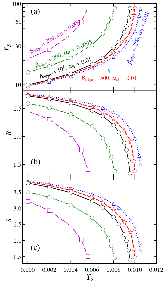
Figure 3: Variations of the shock properties with $\Upsilon_{\rm s}$ for various values of the $\beta_{\rm edge}$ and $\alpha_{\rm B}$. In panel (a), we plot the shock radius ($r_{\rm s}$); in panel (b), the compression ratio ($R$), and in panel (c), we illustrate the shock strength ($S$). We choose $\alpha_{\rm B}=0.01$, and $a_{\rm{k}}=0.99$. See the text for details.

Next, we compare the size of the post-shock corona (PSC) by examining the shock radius ($r_{\rm s}$) as a function of conduction parameter ($\Upsilon_{\rm s}$) for flows with varying viscosity ($\alpha_{\rm B}$) and magnetic field strengths ($\beta_{\rm edge}$). Here, matter is injected from $r_{\rm edge}=500$ with $\mathcal{E}_{\rm edge}=1.00105$ and $\lambda_{\rm edge}=2.266$ onto a black hole with spin $a_{\rm k}=0.99$. Initially, we fix $\beta_{\rm edge}=200$ at $r_{\rm edge}=500$ and vary $\alpha_{\rm B}$. The obtained results are presented in Fig. 3(a), where open squares, circles and triangles connected with lines correspond to $\alpha_{\rm B}=0.009$, $0.0095$ and $0.01$, respectively. We observe that for a fixed $\beta_{\rm{edge}}$ and $\alpha_{\rm B}$, the shock radius $r_{\rm{s}}$ moves away from the horizon as $\Upsilon_{\rm s}$ is increased. However, when thermal conduction exceeds its critical value ($\Upsilon_{\rm s}>\Upsilon^{\rm cri}_{\rm s}$), the shock disappears as RHCs are not favorable. Furthermore, for a fixed $\Upsilon_{\rm s}$, as $\alpha_{\rm B}$ increases, the shock settles down to a smaller radius due the weakening of the centrifugal repulsion, that results because of the more efficient angular momentum transport. Thereafter, we examine the effect of magnetic field on shock formation. We observe that for gas pressure dominated flow ($i.e.$, $\beta_{\rm edge}=10^{4}$) with $\alpha_{\rm B}=0.01$, the shock forms further from the black hole at a given $\Upsilon_{\rm s}$. As the magnetic field strength increases ($i.e.$ as $\beta_{\rm edge}$ decreases), the shock radius $r_{\rm s}$ proceeds towards the black hole. The open circles and asterisks joined with solid and dashed lines represent the variation of $r_{\rm s}$ with $\Upsilon_{\rm s}$ for $\beta_{\rm edge}=10^{4}$ and $\beta_{\rm edge}=500$, respectively. Indeed, the disc’s high energy radiation flux is primarily determined by radiative cooling processes, which are strongly dependent on the density $\rho$ and temperature $T$ distributions across the shock front Chakrabarti and Titarchuk (1995) Mandal and Chakrabarti (2005). Accordingly, in Fig. 3b, we illustrate the variation of the compression ratio $(R)$, which quantifies density compression across the shock, as a function of $\Upsilon_{\rm s}$ for the shock-induced accretion solutions presented in Fig. 3a. As $\Upsilon_{\rm s}$ increases, the shock generally moves away from the black hole horizon, causing the post-shock region (PSC) to experience less compression and leading to a decrease in the compression ratio $R$. In a way, the shock becomes weaker in the presence of thermal conduction. In contrast, when $\beta_{\rm edge}$ decreases, the shock front moves inward toward the black hole, which results in greater compression of the PSC and, consequently, an increase in $R$. In addition, we also examine the variation of shock strength $S$ as a function of $\Upsilon_{\rm s}$ for the solutions presented in Fig. 3a and observe that $S$ decreases as thermal conduction is increased, as shown in Fig. 3c. Based on these finding, it is evident that shock-induced global accretion solutions exist across a wide range of $\Upsilon_{\rm s}$ for various values of $\beta_{\rm edge}$ and $\alpha_{\rm B}$. Notably, these shock-driven accretion solutions have been successful in explaining the observed spectro-temporal characteristics of black hole X-ray binary sources, as demonstrated in numerous studies Chakrabarti and Titarchuk (1995); Chakrabarti and Manickam (2000); Mandal and Chakrabarti (2005); Nandi et al. (2012); Iyer et al. (2015); Das et al. (2021); Majumder et al. (2022); Nandi et al. (2024).

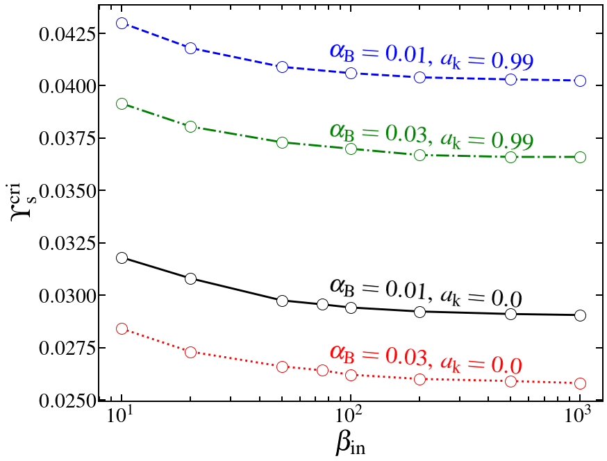
Figure 4: Plot of $\Upsilon_{\rm s}^{\rm{cri}}$ with the $\beta_{\rm{in}}$ for various values of $\alpha_{\rm{B}}$ for non-rotating ($a_{\rm{k}}=0.0$) and maximally rotating ($a_{\rm{k}}=0.99$) BHs. Here, $\Upsilon_{\rm s}^{\rm{cri}}$ is the limiting value of the $\Upsilon_{\rm s}$ beyond which shock solutions cease to exist; see text for details.

It is evident that global shock-induced accretion solutions exist within a specific range of the conduction parameter $\Upsilon_{\rm s}$ which is bounded by its critical value $\Upsilon^{\rm cri}_{\rm s}$. Notably, $\Upsilon^{\rm cri}_{\rm s}$ does not have a universal value; instead, it depends on the other model parameters. To explore this, we calculate $\Upsilon^{\rm cri}_{\rm s}$ for both weakly rotating ($a_{\rm k}\rightarrow 0$) and rapidly rotating ($a_{\rm k}\rightarrow 1$)black holes, and investigate how it varies with the magnetic field strength at the inner critical point. Since the inner critical points ($r_{\rm in}$) are located close to the horizon, it is reasonable to assume that the flow enters into the black hole with magnetic fields ($\beta$) similar to those at the inner critical point $\beta_{\rm in}$. Hence, we examine the variation of $\Upsilon^{\rm cri}_{\rm s}$ with $\beta_{\rm in}$ for different $\alpha_{\rm B}$ values and depict the obtained results in Fig. 4. It is important to note that while calculating $\Upsilon^{\rm cri}_{\rm s}$, we freely vary the remaining model parameters. We observe that $\Upsilon^{\rm cri}_{\rm s}$ increases as the magnetic field strength increaes ($i.e.$ as $\beta_{\rm in}$ decreases) regardless of the black hole spin ($a_{\rm k}$). In addition, higher viscosity leads to lower values of $\Upsilon^{\rm cri}_{\rm s}$. Furthermore, we notice that for a given set of ($\beta_{\rm in},\alpha_{\rm B}$), $\Upsilon^{\rm cri}_{\rm s}$ is larger for higher black hole spin $a_{\rm k}$ and smaller for lower $a_{\rm k}$.

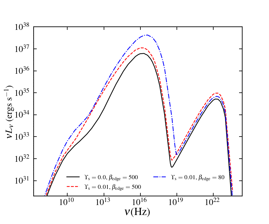
Figure 5: Spectral energy distribution (SED) of accretion solutions for different conduction parameter ($\Upsilon_{\rm s}$) and plasma-$\beta$. Solid (black), dashed (red) and dot-dashed curves denote results for ($\Upsilon_{\rm s},\beta_{\rm edge}$) $=(0.0,500)$, $(0.01,500)$ and $(0.01,80)$, respectively. See the text for details.

Furthermore, we put efforts to calculate the monochromatic luminosity. For a convergent shocked accretion flow, we obtain,

$$L_{\nu}=2\int_{r_{\rm edge}}^{r_{\rm h}}\int_{0}^{2\pi}Q^{-}_{\nu}Hr\thickspace drd\phi\thickspace\thickspace{\rm erg}\thickspace{\rm s}^{-1}{\rm Hz}^{-1},$$ (15)

where $Q^{-}_{\nu}$ refers the total emissivity from at a emission frequency $\nu$. We calculate total emissivity by combining both bremsstrahlung and synchrotron emissivities Novikov and Thorne (1973); Rybicki and Lightman (1986); Wardziński and Zdziarski (2000) as $Q^{-}_{\nu}=Q_{\nu}^{\rm syn}+Q_{\nu}^{\rm brem}$, which are given by,

$$Q_{\nu}^{\rm brem} =6.8\times 10^{-38}n_{e}^{2}T_{e}^{-1/2}$$

$$\times(1+4.4\times 10^{-10}T_{e})\exp\left(\frac{h\nu}{k_{B}T_{e}}\right)\quad{\rm and}$$

$$Q_{\nu}^{\rm syn} =\frac{2^{1/6}\pi^{3/2}e^{2}n_{e}\nu}{3^{5/6}cK_{2}(1/\Theta)u^{1/6}}\exp\left[-\left(\frac{9u}{2}\right)^{1/3}\right],$$

where $u=2\pi m_{e}c\nu/(eB\Theta^{2})$, and $K_{2}(1/\Theta)$ is modified Bessel function of order two.

In this work, we consider strong coupling between electrons and ions, that results in single temperature accretion flow. However, in a realistic scenario, since electrons are much lighter than ions, the electron temperature ($T_{e}$) must be lower than the ion temperature ($T_{i}=T$), at least near the vicinity of the black hole. To account this, we follow the work of Chattopadhyay and Chakrabarti (2000) and estimate the electron temperature as $T_{e}=\sqrt{(m_{e}/m_{i})}T$, where $m_{i}$ and $m_{e}$ are the masses of ions and electrons, respectively. Using Eq. (15), we calculate the spectral energy distribution (SED) for three different shock-induced accretion solutions with varying $\Upsilon_{\rm s}$ and $\beta_{\rm edge}$ values. The results are shown in Fig. 5, where the variation of $\nu L_{\nu}$ with frequency $\nu$ is plotted. Solid (black), dashed (red), and dot-dashed (blue) curves represent the results corresponds to $(\Upsilon_{\rm s},\beta_{\rm edge})=(0.0,500)$, $(0.01,500)$, and $(0.01,80)$, respectively. We observe that for all cases, synchrotron photons dominate the lower energy part of the spectrum, peaking around $\nu\sim 10^{16}$ Hz, while bremsstrahlung photons contribute to the high-energy part, peaking at $\nu\sim 10^{22}$ Hz. The spectra exhibit a sharp cutoff at $\nu\approx 10^{23}$ Hz, corresponding to an electron temperature $T_{e}\approx 10^{10}$ K at the inner edge ($r\sim r_{\rm h}$) of the . We find that the peaks of the SEDs are largely insensitive to effect of the thermal conduction ($\Upsilon_{\rm s}$); however, the synchrotron peaks shift to higher frequencies as the becomes more magnetized ($i.e.$, smaller $\beta_{\rm edge}$). We also observe that the SED is influenced by thermal conduction ($\Upsilon_{\rm s}$), which eventually enhances the disc luminosity. Interestingly, as the magnetic activity increases within the disc, the hot accreting plasma produces more luminous power spectra compared to a weakly magnetized disc.

IV Conclusion

In this study, we examine the impact of thermal conduction and plasma-$\beta$ on global, transonic, magnetized, viscous, advective accretion flows around rotating black holes in presence of bremsstrahlung and synchrotron cooling processes. In this formalism, accretion disc is threaded by the toroidal magnetic fields and the spacetime geometry is mimicked by the effective potential introduced by Dihingia et al. (2018). Furthermore, we adopt relativistic equation of state (REoS) to describe the thermodynamical flow variables. With this, we solve the governing equations that describe the flow motion in accretion disc and obtain the shock-induced global transonic accretion for set of model parameters, namely accretion rate ($\dot{m}$), viscosity parameter ($\alpha_{\rm{B}}$), black hole spin ($a_{\rm k}$), conduction parameter ($\Upsilon_{\rm s}$), plasma-$\beta$, energy and angular momentum of the flow. Our results establish that magnetic fields and thermal conduction play crucial role in regulating the shock phenomena, influencing shock location ($r_{\rm{s}}$), compression ratio ($R$), and shock strength ($S$), which in turn alters the emission spectrum of the disc. The key findings of this study are outlined as follows:

• We find that global transonic magnetized accretion flows undergo shock transitions when thermal conduction is active within the disc. This shock triggering naturally leads to the formation of a hot and dense post-shock flow, which resembles a post-shock corona (PSC) (see Fig. 1). At the PSC, soft photons from the pre-shock flow can be reprocessed, resulting in the production of hard X-rays, which are commonly observed from black hole sources Chakrabarti and Titarchuk (1995); Mandal and Chakrabarti (2005).

• We observe that both thermal conduction and magnetic fields play a pivotal role in shock formation. In particular, thermal conduction exerts an effect opposite to that of magnetic fields in determining the shock transition (see Fig. 2). In addition, we find that shocks continue to form in the accretion flow across a wide range of conduction parameter $\Upsilon_{\rm s}$ and plasma-$\beta$, including the viscosity parameter $\alpha_{\rm B}$. In a way, shock transitions are driven by the synergistic interplay between thermal conduction, viscosity, and magnetic fields. These factors collectively influence the shock properties and determine the disc structure of the accretion flow. Moreover, we notice that for all cases, strong shocks are formed when $\Upsilon_{\rm s}$ is small, with shock strength diminishing as $\Upsilon_{\rm s}$ increases (see Fig. 3).

• We calculate the critical conduction parameter $\Upsilon^{\rm cri}_{\rm s}$ that renders global shocked magnetized accretion solutions around both weakly rotating ($a_{\rm k}\rightarrow 0$) as well as rapidly rotating ($a_{\rm k}\rightarrow 1$) black holes. Our results reveal that accretion flows around rapidly rotating black holes can sustain higher values of $\Upsilon^{\rm cri}_{\rm s}$ compared to weakly rotating black holes, independent of magnetic field strengths in the inner disc region ($i.e.$, plasma-$\beta$). Furthermore, for a fixed $a_{\rm k}$ and $\beta_{\rm in}$, we find that $\Upsilon^{\rm cri}_{\rm s}$ is larger for weakly viscous flows and decreases with increasing viscosity (see Fig. 4).

• We examine the impact of the conduction parameter $\Upsilon_{\rm s}$ and plasma-$\beta$ on the disc emission spectrum (SEDs) resulted due to the bremsstrahlung and synchrotron cooling processes. Our findings indicate that the inclusion of thermal conduction noticeably enhances the emission spectrum. Moreover, we observe that increased magnetic activity also leads to more luminous emission spectrum (see Fig. 5).

Finally, we wish to emphasize that the current formalism is developed under several simplifying assumptions. We approximate the spacetime geometry adopting an effective pseudo-potential instead of a full general relativistic treatment. Our analysis focuses exclusively on the toroidal component of the magnetic field, neglecting the poloidal components and the effects of anisotropic thermal conduction in complex magnetic field configurations. Moreover, we neglect mass loss from the disc, even though thermal conduction may play a significant role in driving outflows and/or winds. While all these processes are relevant in accretion dynamics, their inclusion is beyond the scope of this paper and will be explored in future studies.

Data Availability

The data underlying this paper will be available with reasonable request.

Appendix A Calculation of wind equation

After some algebraic manipulation, the equations for radial momentum, azimuthal momentum, and entropy generation are expressed as follows:

$$R_{0}+R_{\Theta}\frac{d\Theta}{dr}+R_{\lambda}\frac{d\lambda}{dr}+R_{\beta}\frac{d\beta}{dr}+R_{\upsilon}\frac{d\upsilon}{dr}=0,$$ (16)

$$L_{0}+L_{\Theta}\frac{d\Theta}{dr}+L_{\lambda}\frac{d\lambda}{dr}+L_{\beta}\frac{d\beta}{dr}+L_{\upsilon}\frac{d\upsilon}{dr}=0,$$ (17)

$$B_{0}+B_{\Theta}\frac{d\Theta}{dr}+B_{\lambda}\frac{d\lambda}{dr}+B_{\beta}\frac{d\beta}{dr}+B_{\upsilon}\frac{d\upsilon}{dr}=0,$$ (18)

$$E_{0}+E_{\Theta}\frac{d\Theta}{dr}+E_{\lambda}\frac{d\lambda}{dr}+E_{\beta}\frac{d\beta}{dr}+E_{\upsilon}\frac{d\upsilon}{dr}=0.$$ (19)

Simplifying the above equations, we have,

$$\frac{d\upsilon}{dr}=\frac{\mathcal{N}(r,\upsilon,\lambda,\Theta)}{\mathcal{D}(r,\upsilon,\lambda,\Theta)}$$ (20)

$$\frac{d\Theta}{dr}=\Theta_{\textrm{1}}+\Theta_{\textrm{2}}\frac{d\upsilon}{dr}$$ (21)

$$\frac{d\lambda}{dr}=\lambda_{\textrm{1}}+\lambda_{\textrm{2}}\frac{d\upsilon}{dr}$$ (22)

$$\frac{d\beta}{dr}=\beta_{\textrm{1}}+\beta_{\textrm{2}}\frac{d\upsilon}{dr},$$ (23)

where,

$$\mathcal{N}(r,\upsilon,\lambda,\Theta)=-E_{\beta}R_{\lambda}B_{\Theta}B_{0}+E_{\beta}R_{\Theta}B_{\lambda}L_{0}$$

$$+E_{0}R_{\lambda}B_{\Theta}L_{\beta}-E_{0}R_{\Theta}B_{\lambda}B_{\beta}+E_{\beta}R_{\lambda}B_{0}L_{\Theta}$$

$$-E_{0}R_{\lambda}B_{\beta}L_{\Theta}-E_{\beta}R_{0}B_{\lambda}L_{\Theta}+E_{0}R_{\beta}B_{\lambda}L_{\Theta}$$

$$+E_{\lambda}[R_{\beta}B_{\Theta}L_{0}-R_{0}B_{\Theta}L_{\beta}+R_{\Theta}(-B_{\beta}L_{0}+B_{0}L_{\beta})$$

$$-R_{\beta}B_{0}L_{\Theta}+R_{0}B_{\beta}L_{\Theta}]-E_{\beta}R_{0}B_{0}L_{\lambda}+E_{0}R_{\Theta}B_{\beta}L_{\lambda}$$

$$+E_{\beta}R_{0}B_{\Theta}B_{\lambda}-E_{0}R_{\beta}B_{\Theta}L_{\lambda}+E_{\Theta}[R_{\lambda}B_{\beta}L_{0}$$

$$-R_{\beta}B_{\lambda}L_{0}-R_{\lambda}B_{0}L_{\beta}+R_{0}B_{\lambda}L_{\beta}+R_{\beta}B_{0}L_{\lambda}$$

$$-R_{0}B_{\beta}L_{\lambda}],$$

$$\mathcal{D}(r,\upsilon,\lambda,\Theta)=E_{\beta}R_{\lambda}B_{\theta}L_{\upsilon}-E_{\beta}R_{\Theta}B_{\lambda}L_{\upsilon}$$

$$-E_{\upsilon}R_{\lambda}B_{\Theta}L_{\beta}+E_{\upsilon}R_{\Theta}B_{\lambda}L_{\beta}-E_{\beta}R_{\lambda}B_{\upsilon}L_{\Theta}$$

$$+E_{\upsilon}R_{\lambda}B_{\beta}L_{\Theta}+E_{\beta}R_{\upsilon}B_{\lambda}L_{\Theta}-E_{\upsilon}R_{\beta}B_{\lambda}L_{\Theta}$$

$$+E_{\lambda}[-R_{\beta}B_{\Theta}L_{\upsilon}+R_{\upsilon}B_{\Theta}L_{\beta}+R_{\Theta}(B_{\beta}L_{\upsilon}$$

$$-B_{\upsilon}L_{\beta})+R_{\beta}B_{\upsilon}L_{\Theta}-R_{\upsilon}B_{\beta}L_{\Theta}]+E_{\beta}R_{\Theta}B_{\upsilon}L_{\lambda}$$

$$-E_{\upsilon}R_{\Theta}B_{\beta}L_{\lambda}-E_{\beta}R_{\upsilon}B_{\Theta}L_{\lambda}+E_{\upsilon}R_{\beta}B_{\Theta}L_{\lambda}$$

$$+E_{\Theta}[-R_{\lambda}B_{\beta}L_{\upsilon}+R_{\beta}B_{\lambda}L_{\upsilon}+R_{\lambda}B_{\upsilon}L_{\beta}$$

$$-R_{\upsilon}B_{\lambda}L_{\beta}-R_{\beta}B_{\upsilon}L_{\lambda}+R_{\upsilon}B_{\beta}L_{\lambda}]$$

$$\Theta_{1} =\frac{\Theta_{11}}{\Theta_{33}},\thickspace\Theta_{2}=\frac{\Theta_{22}}{\Theta_{33}},\thickspace\lambda_{1}=\frac{\lambda_{11}}{\lambda_{33}},\thickspace\lambda_{2}=\frac{\lambda_{22}}{\lambda_{33}},$$

$$\beta_{1} =\frac{\beta_{11}}{\beta_{33}},\thickspace\beta_{2}=\frac{\beta_{22}}{\beta_{33}},$$

$$\Theta_{11} =-[(E_{\beta}L_{0}-E_{0}L_{\beta})(E_{\lambda}B_{\beta}-E_{\beta}B_{\lambda})$$

$$+(-E_{\lambda}L_{\beta}+E_{\beta}L_{\lambda})(E_{\beta}B_{0}-E_{0}B_{\beta})],$$

$$\Theta_{22} =-[(E_{\beta}L_{\upsilon}-E_{\upsilon}L_{\beta})(E_{\lambda}B_{\beta}-E_{\beta}B_{\lambda})$$

$$+(E_{\beta}\beta_{\upsilon}-E_{\upsilon}B_{\beta})(-E_{\lambda}L_{\beta}+E_{\beta}L_{\lambda})],$$

$$\Theta_{33} =(E_{\lambda}B_{\beta}-E_{\beta}B_{\lambda})(-E_{\Theta}L_{\beta}+E_{\beta}L_{\Theta})$$

$$+(-E_{\Theta}B_{\beta}+E_{\beta}\beta_{\Theta})(-E_{\lambda}L_{\beta}+E_{\beta}L_{\lambda}),$$

$$\lambda_{11} =-E_{\Theta}B_{\beta}L_{0}+E_{\beta}B_{\Theta}L_{0}+E_{\Theta}B_{0}L_{\beta}-E_{0}B_{\Theta}L_{\beta},$$

$$-E_{\beta}B_{0}L_{\Theta}+E_{0}B_{\beta}L_{\Theta},$$

$$\lambda_{22} =-E_{\Theta}B_{\beta}L_{\upsilon}+E_{\beta}B_{\Theta}L_{\upsilon}+E_{\Theta}B_{\upsilon}L_{\beta}-E_{\upsilon}B_{\Theta}L_{\beta},$$

$$-E_{\beta}B_{\upsilon}L_{\Theta}+E_{0}B_{\beta}L_{\Theta},$$

$$\lambda_{33} =E_{\lambda}B_{\Theta}L_{\beta}-E_{\Theta}B_{\lambda}L_{\beta}-E_{\lambda}B_{\beta}L_{\Theta}+E_{\beta}B_{\lambda}L_{\Theta}$$

$$+E_{\Theta}B_{\beta}L_{\lambda}-E_{\beta}B_{\Theta}L_{\lambda},$$

$$\beta_{11} =-E_{\lambda}B_{\Theta}L_{0}+E_{\Theta}B_{\lambda}L_{0}+E_{\lambda}B_{0}L_{\Theta}-E_{0}B_{\lambda}L_{\Theta}$$

$$-E_{\Theta}B_{0}L_{\lambda}+E_{0}B_{\Theta}L_{\lambda},$$

$$\beta_{22} =-E_{\lambda}B_{\Theta}L_{\upsilon}+E_{\Theta}B_{\lambda}L_{\upsilon}+E_{\lambda}B_{\upsilon}L_{\Theta}-E_{\upsilon}B_{\lambda}L_{\Theta}$$

$$-E_{\Theta}B_{\upsilon}L_{\lambda}+E_{\upsilon}B_{\Theta}L_{\lambda},$$

$$\beta_{33} =\lambda_{33},$$

$$R_{0} =\frac{4\Theta}{r\beta\tau}+\frac{2\Theta(1+\beta^{-1})}{\tau h}\left(-\frac{3}{2r}+\frac{F_{3}}{2F_{2}}-\frac{1}{2\Delta}\frac{d\Delta}{dr}\right)$$

$$+\frac{d\Psi_{\rm{e}}^{\rm{eff}}}{dr},R_{\upsilon}=\upsilon-\frac{2\Theta}{\tau h\upsilon}(1+\beta^{-1}),$$

$$R_{\Theta} =\frac{(1+\beta^{-1})}{\tau h},R_{\lambda}=\frac{F_{4}\Theta(1+\beta^{-1})}{\tau hF_{2}},R_{\beta}=-\frac{\Theta}{\tau h\beta^{2}},$$

$$L_{0} =-2\alpha_{\rm{B}}\upsilon^{2}-\frac{4\alpha_{\rm{B}}\Theta(1+\beta^{-1})}{\tau}$$

$$+\frac{d\Delta}{dr}\left(\frac{r\alpha_{\rm{B}}(\tau\upsilon^{2}\beta+2\Theta(1+\beta^{-1}))}{2\tau\beta}\right),$$

$$L_{\upsilon} =-r\alpha_{\rm{B}}\upsilon+\frac{2r\alpha_{\rm{B}}\Theta(1+\beta^{-1})}{\tau\upsilon},$$

$$L_{\Theta} =-\frac{2r\alpha_{\rm{B}}(1+\beta^{-1})}{\tau},$$

$$L_{\lambda} =\upsilon,\thickspace L_{\beta}=\frac{2r\alpha\Theta}{\tau\beta^{2}},$$

$$E_{0} =-\frac{Q^{-}}{\rho H}+\frac{5\Upsilon_{\rm s}\Theta}{\tau}\sqrt{\frac{2\Theta}{\tau}}\left(\frac{1}{r}-\frac{F_{3}}{F_{2}}+\frac{1}{\Delta}\frac{d\Delta}{dr}\right)$$

$$+\frac{3\upsilon\Theta}{r\tau}-\frac{F_{3}\upsilon\Theta}{\tau F_{2}}-\frac{2r\alpha_{\rm{B}}\Theta\omega_{1}(1+\beta^{-1})}{\tau}$$

$$-r\alpha_{\rm{B}}\upsilon^{2}\omega_{1}+\frac{\upsilon\Theta}{\tau\Delta}\frac{d\Delta}{dr},$$

$$E_{\upsilon} =\frac{2\Theta}{\tau}+\frac{10\sqrt{2}\Upsilon_{\rm s}}{\upsilon}\left(\frac{\Theta}{\tau}\right)^{3/2},$$

$$E_{\Theta} =-\frac{5\Upsilon_{\rm s}}{\Theta}\left(\frac{2\Theta}{\tau}\right)^{3/2}+\frac{\left(1+2N\right)\upsilon}{\tau},$$

$$E_{\lambda} =-\frac{F_{4}\upsilon\Theta}{\tau F_{2}}-\frac{5\sqrt{2}\Upsilon_{\rm s}F_{4}}{F_{2}}\left(\frac{\Theta}{\tau}\right)^{3/2}$$

$$-r\alpha_{\rm{B}}\left(\upsilon^{2}+\frac{2\Theta(1+\beta^{-1})}{\tau}\right)\omega_{2},$$

$$E_{\beta}=-\frac{1}{\beta(1+\beta)}\left(\frac{\upsilon\Theta}{\tau}+\frac{5\Upsilon_{\rm s}\Theta}{\tau}\sqrt{\frac{2\Theta}{\tau}}\right),$$

$$B_{0}=\frac{3}{4r}+\frac{\zeta}{r}-\frac{F_{3}}{4F_{2}}-\frac{1}{4\Delta}\frac{d\Delta}{dr},\thickspace B_{\upsilon}=\frac{1}{2\upsilon},B_{\Theta}=\frac{3}{4\Theta},$$

$$B_{\lambda}=-\frac{F_{4}}{4F_{2}},\thickspace B_{\beta}=-\frac{1}{(1+\beta)}\left(\frac{1}{2}+\frac{3}{4\beta}\right),$$

$$F_{3}=\frac{F_{1}\lambda\omega_{1}}{(1-\lambda\Omega)^{2}}+\frac{1}{1-\lambda\Omega}\frac{dF_{1}}{dr},$$

$$F_{4}=\frac{F_{1}\Omega}{(1-\lambda\Omega)^{2}}+\frac{F_{1}\lambda\omega_{2}}{(1-\lambda\Omega)^{2}},$$

$$F_{2}=\frac{1}{(1-\lambda\Omega)}F_{1},$$

$$F_{1}=\frac{\left((r^{2}+a_{\textrm{k}}^{2})^{2}+2\Delta a_{\textrm{k}}^{2}\right)}{\left((r^{2}+a_{\textrm{k}}^{2})^{2}-2\Delta a_{\textrm{k}}^{2}\right)},$$

$$\frac{dF_{2}}{dr}=F_{3}+F_{4}\frac{d\lambda}{dr},\thickspace\frac{d\Omega}{dr}=\omega_{1}+\omega_{2}\frac{d\lambda}{dr},$$

$$\omega_{1}=-\frac{2\left(a_{\textrm{k}}^{3}+3a_{\textrm{k}}r^{2}+\lambda(a_{\textrm{k}}\lambda-2a_{\textrm{k}}^{2}+r^{2}(r-3))\right)}{\left(r^{3}+a_{\textrm{k}}^{2}(r+2)-2a_{\textrm{k}}\lambda\right)^{2}},$$

$$\omega_{2}=\frac{r^{2}\left(a_{\textrm{k}}^{2}+r(r-2)\right)}{\left(r^{3}+a_{\textrm{k}}^{2}(r+2)-2a_{\textrm{k}}\lambda\right)^{2}}.$$

References

- Remillard and McClintock (2006) R. A. Remillard and J. E. McClintock, ARA&A 44, 49 (2006), eprint astro-ph/0606352.
- Netzer (2013) H. Netzer, The Physics and Evolution of Active Galactic Nuclei (2013).
- Event Horizon Telescope Collaboration et al. (2022) Event Horizon Telescope Collaboration, K. Akiyama, A. Alberdi, W. Alef, J. C. Algaba, R. Anantua, K. Asada, R. Azulay, U. Bach, A.-K. Baczko, et al., ApJ 930, L16 (2022).
- Event Horizon Telescope Collaboration et al. (2021) Event Horizon Telescope Collaboration, K. Akiyama, J. C. Algaba, A. Alberdi, W. Alef, R. Anantua, K. Asada, R. Azulay, A.-K. Baczko, D. Ball, et al., ApJ 910, L13 (2021), eprint 2105.01173.
- Narayan and Yi (1994) R. Narayan and I. Yi, ApJ 428, L13 (1994), eprint astro-ph/9403052.
- Narayan and Yi (1995) R. Narayan and I. Yi, ApJ 452, 710 (1995), eprint astro-ph/9411059.
- Yuan and Narayan (2014) F. Yuan and R. Narayan, ARA&A 52, 529 (2014), eprint 1401.0586.
- Ho (2008) L. C. Ho, ARA&A 46, 475 (2008), eprint 0803.2268.
- Oda et al. (2007) H. Oda, M. Machida, K. E. Nakamura, and R. Matsumoto, PASJ 59, 457 (2007), eprint astro-ph/0701658.
- Sarkar and Das (2016) B. Sarkar and S. Das, MNRAS 461, 190 (2016), eprint 1606.00526.
- Das and Sarkar (2018) S. Das and B. Sarkar, MNRAS 480, 3446 (2018), eprint 1807.11417.
- Jana and Das (2024) C. Jana and S. Das, Journal of Cosmology and Astroparticle Physics 2024, 075 (2024), URL https://dx.doi.org/10.1088/1475-7516/2024/07/075.
- Tanaka and Menou (2006) T. Tanaka and K. Menou, ApJ 649, 345 (2006), eprint astro-ph/0604509.
- Johnson and Quataert (2007) B. M. Johnson and E. Quataert, ApJ 660, 1273 (2007), eprint astro-ph/0608467.
- Sharma et al. (2008) P. Sharma, E. Quataert, and J. M. Stone, MNRAS 389, 1815 (2008), eprint 0804.1353.
- Shadmehri (2008) M. Shadmehri, Astrophysics and Space Science 317, 201 (2008), eprint 0808.0245.
- Faghei (2012) K. Faghei, MNRAS 420, 118 (2012), eprint 1111.3569.
- Khajenabi and Shadmehri (2013) F. Khajenabi and M. Shadmehri, MNRAS 436, 2666 (2013), eprint 1309.5710.
- Ghoreyshi and Shadmehri (2020) S. M. Ghoreyshi and M. Shadmehri, Monthly Notices of the Royal Astronomical Society 493, 5107 (2020), eprint 2003.04752.
- Mitra et al. (2023) S. Mitra, S. M. Ghoreyshi, A. Mosallanezhad, S. Abbassi, and S. Das, Monthly Notices of the Royal Astronomical Society 523, 4431 (2023), eprint 2306.02453.
- Landau and Lifshitz (1959) L. D. Landau and E. M. Lifshitz, Fluid mechanics (1959).
- Becker and Kazanas (2001) P. A. Becker and D. Kazanas, ApJ 546, 429 (2001), eprint astro-ph/0101020.
- Mitra and Das (2024) S. Mitra and S. Das, ApJ 971, 28 (2024), eprint 2405.16326.
- Fukue (1987) J. Fukue, PASJ 39, 309 (1987).
- Chakrabarti (1989) S. K. Chakrabarti, ApJ 347, 365 (1989).
- Chakrabarti and Molteni (1993) S. K. Chakrabarti and D. Molteni, ApJ 417, 671 (1993), eprint astro-ph/9310042.
- Molteni et al. (1994) D. Molteni, G. Lanzafame, and S. K. Chakrabarti, ApJ 425, 161 (1994), eprint astro-ph/9310047.
- Yang and Kafatos (1995) R. Yang and M. Kafatos, A&A 295, 238 (1995).
- Chakrabarti (1996) S. K. Chakrabarti, ApJ 464, 664 (1996), eprint astro-ph/9606145.
- Molteni et al. (1996) D. Molteni, D. Ryu, and S. K. Chakrabarti, ApJ 470, 460 (1996), eprint astro-ph/9605116.
- Ryu et al. (1997) D. Ryu, S. K. Chakrabarti, and D. Molteni, ApJ 474, 378 (1997), eprint astro-ph/9607051.
- Lanzafame et al. (1998) G. Lanzafame, D. Molteni, and S. K. Chakrabarti, MNRAS 299, 799 (1998), eprint astro-ph/9706248.
- Lu et al. (1999) J.-F. Lu, W.-M. Gu, and F. Yuan, ApJ 523, 340 (1999), eprint astro-ph/9905099.
- Das et al. (2001) S. Das, I. Chattopadhyay, and S. K. Chakrabarti, ApJ 557, 983 (2001), eprint astro-ph/0107046.
- Chakrabarti and Das (2004) S. K. Chakrabarti and S. Das, MNRAS 349, 649 (2004), eprint astro-ph/0402561.
- Le and Becker (2004) T. Le and P. A. Becker, ApJ 617, L25 (2004), eprint astro-ph/0411801.
- Fukumura and Tsuruta (2004) K. Fukumura and S. Tsuruta, ApJ 611, 964 (2004), eprint astro-ph/0405269.
- Takahashi et al. (2006) M. Takahashi, J. Goto, K. Fukumura, D. Rilett, and S. Tsuruta, ApJ 645, 1408 (2006), eprint astro-ph/0511217.
- Das (2007) S. Das, MNRAS 376, 1659 (2007), eprint astro-ph/0610651.
- Fukumura et al. (2007) K. Fukumura, M. Takahashi, and S. Tsuruta, ApJ 657, 415 (2007), eprint astro-ph/0602568.
- Becker et al. (2008) P. A. Becker, S. Das, and T. Le, ApJ 677, L93 (2008), eprint 0907.0872.
- Das et al. (2009) S. Das, P. A. Becker, and T. Le, ApJ 702, 649 (2009), eprint 0907.0875.
- Kumar et al. (2013) R. Kumar, C. B. Singh, I. Chattopadhyay, and S. K. Chakrabarti, MNRAS 436, 2864 (2013), eprint 1310.0144.
- Das et al. (2014) S. Das, I. Chattopadhyay, A. Nandi, and D. Molteni, MNRAS 442, 251 (2014), eprint 1405.4415.
- Okuda and Das (2015) T. Okuda and S. Das, MNRAS 453, 147 (2015), eprint 1507.04326.
- Suková and Janiuk (2015) P. Suková and A. Janiuk, MNRAS 447, 1565 (2015), eprint 1411.7836.
- Fukumura et al. (2016) K. Fukumura, D. Hendry, P. Clark, F. Tombesi, and M. Takahashi, ApJ 827, 31 (2016), eprint 1606.01851.
- Suková et al. (2017) P. Suková, S. Charzyński, and A. Janiuk, MNRAS 472, 4327 (2017), eprint 1709.01824.
- Aktar et al. (2017) R. Aktar, S. Das, A. Nandi, and H. Sreehari, MNRAS 471, 4806 (2017), eprint 1707.07511.
- Dihingia et al. (2018) I. K. Dihingia, S. Das, D. Maity, and S. Chakrabarti, Phys. Rev. D 98, 083004 (2018), eprint 1806.08481.
- Dihingia et al. (2019) I. K. Dihingia, S. Das, and A. Nandi, Monthly Notices of the Royal Astronomical Society 484, 3209 (2019), eprint 1901.04293.
- Kim et al. (2019) J. Kim, S. K. Garain, S. K. Chakrabarti, and D. S. Balsara, MNRAS 482, 3636 (2019), eprint 1810.12469.
- Okuda et al. (2019) T. Okuda, C. B. Singh, S. Das, R. Aktar, A. Nandi, and E. M. d. G. Dal Pino, PASJ 71, 49 (2019), eprint 1902.02933.
- Dihingia et al. (2020) I. K. Dihingia, S. Das, G. Prabhakar, and S. Mandal, MNRAS 496, 3043 (2020), eprint 1911.02757.
- Sen et al. (2022) G. Sen, D. Maity, and S. Das, J. Cosmology Astropart. Phys 2022, 048 (2022), eprint 2204.02110.
- Singh and Das (2024a) M. Singh and S. Das, Astrophysics and Space Science 369, 1 (2024a), eprint 2312.16001.
- Singh and Das (2024b) M. Singh and S. Das, arXiv e-prints arXiv:2408.02256 (2024b), eprint 2408.02256.
- Debnath et al. (2024) S. Debnath, I. Chattopadhyay, and R. K. Joshi, MNRAS 528, 3964 (2024), eprint 2401.07786.
- TianLe-Zhao et al. (2024) TianLe-Zhao, XiaoFeng-Li, ZeYuan-Tang, and R. Kumar, arXiv e-prints arXiv:2407.01859 (2024), eprint 2407.01859.
- Patra et al. (2024) S. Patra, B. R. Majhi, and S. Das, J. Cosmology Astropart. Phys 2024, 060 (2024), eprint 2308.12839.
- Chakrabarti and Titarchuk (1995) S. Chakrabarti and L. G. Titarchuk, ApJ 455, 623 (1995), eprint astro-ph/9510005.
- Chakrabarti and Manickam (2000) S. K. Chakrabarti and S. G. Manickam, ApJ 531, L41 (2000), eprint astro-ph/9910012.
- Mandal and Chakrabarti (2005) S. Mandal and S. K. Chakrabarti, A&A 434, 839 (2005).
- Nandi et al. (2012) A. Nandi, D. Debnath, S. Mandal, and S. K. Chakrabarti, A&A 542, A56 (2012), eprint 1204.5044.
- Iyer et al. (2015) N. Iyer, A. Nandi, and S. Mandal, ApJ 807, 108 (2015), eprint 1505.02529.
- Das et al. (2021) S. Das, A. Nandi, V. K. Agrawal, I. K. Dihingia, and S. Majumder, MNRAS 507, 2777 (2021), eprint 2108.02973.
- Majumder et al. (2022) S. Majumder, H. Sreehari, N. Aftab, T. Katoch, S. Das, and A. Nandi, MNRAS 512, 2508 (2022), eprint 2203.02710.
- Nandi et al. (2024) A. Nandi, S. Das, S. Majumder, T. Katoch, H. M. Antia, and P. Shah, MNRAS 531, 1149 (2024), eprint 2404.17160.
- Matsumoto et al. (1984) R. Matsumoto, S. Kato, J. Fukue, and A. T. Okazaki, PASJ 36, 71 (1984).
- Riffert and Herold (1995) H. Riffert and H. Herold, ApJ 450, 508 (1995).
- Peitz and Appl (1997) J. Peitz and S. Appl, MNRAS 286, 681 (1997), eprint astro-ph/9612205.
- Machida et al. (2006) M. Machida, K. E. Nakamura, and R. Matsumoto, PASJ 58, 193 (2006), eprint astro-ph/0511299.
- Shapiro and Teukolsky (1983) S. L. Shapiro and S. A. Teukolsky, Black holes, white dwarfs and neutron stars. The physics of compact objects (1983).
- Rybicki and Lightman (1986) G. B. Rybicki and A. P. Lightman, Radiative Processes in Astrophysics (1986).
- Wardziński and Zdziarski (2000) G. Wardziński and A. A. Zdziarski, MNRAS 314, 183 (2000), eprint astro-ph/9911126.
- Cowie and McKee (1977) L. L. Cowie and C. F. McKee, ApJ 211, 135 (1977).
- Chattopadhyay and Ryu (2009) I. Chattopadhyay and D. Ryu, ApJ 694, 492 (2009), eprint 0812.2607.
- Nandi et al. (2018) A. Nandi, S. Mandal, H. Sreehari, D. Radhika, S. Das, I. Chattopadhyay, N. Iyer, V. K. Agrawal, and R. Aktar, Ap&SS 363, 90 (2018), eprint 1803.08638.
- Frank et al. (2002) J. Frank, A. King, and D. J. Raine, Accretion Power in Astrophysics: Third Edition (Cambridge, UK: Cambridge University Press, 2002).
- Novikov and Thorne (1973) I. D. Novikov and K. S. Thorne, in Black Holes (Les Astres Occlus), edited by C. Dewitt and B. S. Dewitt (1973), pp. 343–450.
- Chattopadhyay and Chakrabarti (2000) I. Chattopadhyay and S. K. Chakrabarti, International Journal of Modern Physics D 9, 717 (2000).