Splitting Regularized Wasserstein Proximal Algorithms
for Nonsmooth Sampling Problems

Abstract.

Sampling from nonsmooth target probability distributions is essential in various applications, including the Bayesian Lasso. We propose a splitting-based sampling algorithm for the time-implicit discretization of the probability flow for the Fokker-Planck equation, where the score function defined as the gradient logarithm of the current probability density function, is approximated by the regularized Wasserstein proximal. When the prior distribution is the Laplace prior, our algorithm is explicitly formulated as a deterministic interacting particle system, incorporating softmax operators and shrinkage operations to efficiently compute the gradient drift vector field and the score function. The proposed formulation introduces a particular class of attention layers in transformer structures, which can sample sparse target distributions. We verify the convergence towards target distributions regarding Rényi divergences under suitable conditions. Numerical experiments in high-dimensional nonsmooth sampling problems, such as sampling from mixed Gaussian and Laplace distributions, logistic regressions, image restoration with $L_{1}$-TV regularization, and Bayesian neural networks, demonstrate the efficiency and robust performance of the proposed method.

1. Introduction

Solving the Bayesian Lasso problem [28] involves sampling from the target distribution

$$\rho^{*}(x)=\frac{1}{Z}\exp\left(-\beta(f(x)+g(x))\right),$$

where $x\in\mathbb{R}^{d}$, $f:\mathbb{R}^{d}\to\mathbb{R}$ is the negative log-likelihood, $g(x)=\lambda\|x\|_{1}$ is the log-density of the Laplace prior for $\lambda>0$, $\beta>0$ is a known parameter, and $Z$ is an unknown normalization constant. The Bayesian Lasso is widely used as it simultaneously conducts parameter estimation and variable selection. It has broad applications in high-dimensional real-world data analysis, including cancer prediction [10], depression symptom diagnosis [27], and Bayesian neural networks [34].

Most algorithms for sampling from $\rho^{*}$ rely on discretizing the overdamped Langevin dynamics. In each iteration, these algorithms evaluate the gradient of the logarithm of target distribution once and plus a Brownian motion perturbation to generate diffusion. However, the time-discretized overdamped Langevin dynamics presents several challenges. First, the gradient of $g$ may not be well-defined, as in the case of $g$ being a $L_{1}$ norm. Second, overdamped Langevin dynamics often perform inefficiently in high-dimensional sampling problems due to the fact that the variance of Brownian motion linearly depends on the dimension.

To address the first challenge, many proximal sampling algorithms, often with splitting techniques, have been extensively studied. [29, 13, 31] use proximal operators to approximate the gradient of nonsmooth log-density. Extended works include methods leveraging a restricted Gaussian oracle (RGO) [22, 8, 24], incorporating both sub-gradient and proximal operators [16], and solving an inexact proximal map at each iteration [2]. For a recent review, see [21]. In these works, the proximal map is often interpreted as a semi-implicit discretization of the Langevin dynamics with respect to the drift term. The present study also employs the proximal operator to approximate the gradient of nonsmooth terms, however, the proposed algorithm is fully deterministic as described below.

Furthermore, to handle the second challenge, instead of considering the time discretization of the Langevin dynamic, we will analyze a deterministic interacting particle system obtained by the time-discretized probability flow ODE. Here, the ODE involves the drift function and the gradient logarithm of the current probability density function, named the score function, which induces the diffusion. Since this approach avoids simulating Brownian motion, it is independent of the sample space dimension. However, accurately approximating the score function presents a challenge of its own.

To approximate the evolution of the score function, [32] derived a closed-form formula using the regularized Wasserstein proximal operator (RWPO). The RWPO is defined as the Wasserstein proximal operator with a Laplacian regularization term (see Section 2 for details). By applying Hopf–Cole transformations, the operator admits a closed-form kernel formula. It has been shown that the RWPO provides a first-order approximation to the evolution of the Fokker–Planck equation [17], leading to an effective score function approximation. The sampling algorithm based on RWPO named backward regularized Wasserstein proximal (BRWP), has been implemented in several studies [32, 18] with different computational strategies. Its backward nature comes from the implicit time discretization of the probability flow ODE for the score function term. However, a key challenge in implementing the BRWP kernel lies in approximating an integral over $\mathbb{R}^{d}$ to compute the denominator term.

In this work, we derive a computationally efficient closed-form update for BRWP without evaluating a high dimensional integral for special nonsmooth functions, such as the $L_{1}$ norm. Following the restricted Gaussian oracle of BRWP with $L_{1}$ function, we derive an explicit formula of the sampling algorithm, in which samples interact with each other following an interacting kernel function. In particular, this kernel function is constructed by shrinkage operators and the softmax functions. Moreover, we also apply the splitting method and proximal updates for sampling problems with nonsmooth target density.

We sketch the algorithm below. For particles $\{x_{i}^{k}\}_{i=1}^{N}$ in the $k$ iteration, when $g(x)=\lambda\|x\|_{1}$, the proposed iterative sampling scheme is

$$x_{i}^{k+\frac{1}{2}}=x_{i}^{k}-h\nabla f(x_{i}^{k})\,,\quad x_{i}^{k+1}=x_{i}^{k+\frac{1}{2}}+\frac{1}{2}\left(S_{\lambda h}(x_{i}^{k+\frac{1}{2}})-\sum_{j=1}^{N}\text{softmax}(U(i,j)_{j})x_{j}^{k+\frac{1}{2}}\right)\,,$$

where $h>0$ is the time step size. The interacting kernel is defined as

$$U(i,j):=-\frac{\beta}{2}\left(\frac{\|x_{i}^{k+\frac{1}{2}}-x_{j}^{k+\frac{1}{2}}\|_{2}^{2}-\|S_{\lambda h}(x_{i}^{k+\frac{1}{2}})-x_{j}^{k+\frac{1}{2}}\|_{2}^{2}}{2h}-\lambda\|S_{\lambda h}(x_{j}^{k+\frac{1}{2}})\|_{1}\right)\,,$$

with

$$\textrm{softmax}(x)=\left(\frac{\exp(x_{j})}{\sum_{\ell=1}^{N}\exp(x_{\ell})}\right)_{1\leq j\leq N}\,,\quad x\in\mathbb{R}^{d}\,.$$

The shrinkage operator $S_{\lambda h}$ takes the form

$$S_{\lambda h}(x):=\operatorname{sign}(x)\operatorname{ReLU}(|x|-\lambda h)\,,$$

with the rectified linear unit (ReLU) function $\operatorname{ReLU}(z)=\max\{z,0\}$ for $z\in\mathbb{R}$. We remake that the shrinkage operator is the proximal map of the $L_{1}$ norm, i.e., $S_{\lambda h}(x)=\operatorname{prox}_{\lambda\|x\|_{1}}^{h}(x)$.

The iterative scheme exhibits an intriguing connection to recent AI methods, particularly transformer architectures, as explored in [6, 15]. The proposed sampling algorithms can be viewed as analogs of multi-attention transformers, incorporating generalized attention layers and the ReLU function. In this framework, each sample $x^{k}_{i}$ acts as a token, while the matrix operator $U$ defines the attention mechanism. A more detailed discussion of the connection between the proposed scheme and attention mechanisms in transformer architectures is provided in Section 2.4.

Compared to algorithms based on splitting the overdamped Langevin dynamics with Brownian motion, as studied in [29, 13, 31, 22, 8, 24], the proposed deterministic approach generally provides a better approximation to the target density empirically, particularly with a small number of particles. It also demonstrates faster convergence in high-dimensional sample spaces, benefiting from adapting the deterministic score function, as established in [17]. Several other works have investigated deterministic interacting particle systems for sampling, including Stein variational gradient descent methods [25] and blob methods [11]. The proposed approach, however, leverages a kernel formulation derived directly from the solution of the Fokker–Planck equation, naturally incorporating information about the underlying dynamics, as reflected in the definition of $U(i,j)$ above. Furthermore, the proposed kernel is closely related to the restricted Gaussian oracle [22] due to the definition of the kernel formula for RWPO and our computational implementation provides an approximation to the restricted Gaussian oracle.

The structure of this paper is as follows. Section 2 presents the derivation of the BRWP-splitting sampling scheme with a detailed algorithm description. In particular, we introduce several kernels, each corresponding to a different particle-based approximation of the initial density. Section 3 demonstrates the convergence of the BRWP-splitting algorithm towards the target density for the Rényi divergence under the Poincaré inequality and suitable conditions. This analysis is based on an interpolation argument and provides a term-by-term bound on the discretization error. Section 4 extends our approach to other regularization terms, specifically $L_{1}$-TV regularization, which integrates primal-dual hybrid gradient descent with the BRWP-splitting algorithm. Finally, Section 5 presents numerical experiments on mixture distributions, Bayesian logistic regression, several imaging applications, and Bayesian neural network training. Proofs and detailed derivations are included in the supplementary material.

2. Regularized Wasserstein Proximal and Splitting Methods for Sampling

We are aiming to draw samples from probability distributions of the form

$$\rho^{*}(x)=\frac{1}{Z}\exp(-\beta(f(x)+\lambda\|x\|_{1}))\,,$$ (1)

where $x\in\mathbb{R}^{d}$, $f:\mathbb{R}^{d}\rightarrow\mathbb{R}$ is $L$-smooth, $\beta=(k_{B}T)^{-1}$ with a temperature constant $T>0$ and the Boltzmann constant $k_{B}$, $\lambda$ is a regularization parameter, and $Z=\int_{\mathbb{R}^{d}}\exp(-\beta(f(y)+\lambda\|y\|_{1}))dy<+\infty$ is an unknown normalization constant.

Sampling from such a distribution is widely used in parameter estimation, particularly under the framework of the Bayesian Lasso problem [28], which simultaneously performs estimation and variable selection. However, the nonsmoothness of the $L_{1}$ norm poses significant challenges in developing theoretically sound and numerically efficient sampling algorithms. Beyond the Bayesian Lasso setting, we are also interested in more general cases where $g(x)$ is a nonsmooth function whose proximal operator is easy to compute. In this case, we consider sampling from the distribution

$$\rho^{*}(x)=\frac{1}{Z}\exp(-\beta(f(x)+g(x)))\,.$$ (2)

2.1. Langevin dynamic and regularized Wasserstein proximal operator

In this section, we review the time discretization of the overdamped Langevin dynamic and regularized Wasserstein proximal operator to motivate the proposed algorithm.

Denote $V=f+g$ for simplicity. To sample from $\rho^{*}$ in (2), a classical approach involves the overdamped Langevin dynamics at time $t$

$$dX_{t}=-\nabla V(X_{t})dt+\sqrt{2\beta^{-1}}dB_{t}\,,$$ (3)

where $X_{t}\in\mathbb{R}^{d}$ is a stochastic process, and $B_{t}$ is the standard Brownian motion in $\mathbb{R}^{d}$. Denote $\rho_{t}$ as the probability density function of $X_{t}$. It is well known that the Kolmogorov forward equation of stochastic process $X_{t}$ satisfies the following Fokker–Planck equation:

$$\frac{\partial\rho_{t}}{\partial t}=\nabla\cdot(\rho_{t}\nabla V)+\beta^{-1}\Delta\rho_{t}=\beta^{-1}\nabla\cdot\left(\rho_{t}\nabla\log\frac{\rho_{t}}{\rho^{*}}\right)\,$$ (4)

where we use the fact that $\rho_{t}\nabla\log\rho_{t}=\nabla\rho_{t}$ and $\nabla\log\rho^{*}=\nabla\log e^{-\beta V}=-\beta\nabla V$.

From the stationary solution of the Fokker–Planck equation, we observe that the invariant distribution of the Langevin dynamics coincides with the target distribution $\rho^{*}$. However, directly applying the overdamped Langevin dynamics (3) to sample from (1) presents several challenges. Firstly, the function $V$ is nonsmooth which creates difficulties in the gradient computation. Secondly, the variance of the Brownian motion depends on the sample space dimension linearly which slows down convergence, posing challenges for high-dimensional sampling tasks.

To address the first issue, for a small stepsize $h>0$, one often utilizes the Moreau envelope

$$g_{h}(x)=\inf_{y\in\mathbb{R}^{d}}\left\{g(y)+\frac{1}{2h}\|x-y\|_{2}^{2}\right\}\,,$$ (5)

which provides a smooth approximation to the nonsmooth function $g$; and the proximal operator

$$\text{prox}_{g}^{h}(x)=\operatorname*{arg\,min}_{y\in\mathbb{R}^{d}}\left\{g(y)+\frac{1}{2h}\|x-y\|_{2}^{2}\right\}\,,$$ (6)

which provides a smooth approximation to the gradient of $g$ based on the relation

$$\nabla g_{h}(x)=\frac{x-\text{prox}_{g}^{h}(x)}{h},\quad\text{for a convex function }g\,.$$ (7)

These tools have been widely applied in nonsmooth sampling problems [24, 36, 13]. In this work, we also employ the proximal operator to approximate the gradient of nonsmooth functions.

Furthermore, to tackle the second challenge which arises from the linear dependence of the variance of Brownian motion and the dimension, we aim to avoid the simulation of Brownian motions in the sampling algorithm. Instead, we consider the evolution of particles $x_{t}\in\mathbb{R}^{d}$ governed by the probability flow ODE:

$$dx_{t}=-\nabla V(x_{t})dt-\beta^{-1}\nabla\log\rho_{t}(x_{t})dt\,.$$ (8)

Here, the diffusion is induced by the score function $\nabla\log\rho_{t}$. While the individual particle trajectories of equation (8) differ from those of stochastic dynamics (3), the Liouville equation of (8) is still the Fokker–Planck equation (4).

The primary challenge in discretizing the probability flow ODE (8) in time is the accurate approximation of the score function. For each discretized time point, since we can only access $N$ particles obtained from the previous iteration, kernel density estimation-based particle methods can be unstable and sensitive to the choice of bandwidth. To mitigate this, we consider a semi-implicit discretization of (8), where the score function at the next time step is utilized. This results in the following iterative sampling scheme.

Denote the time steps as $t_{k}$ for $k=1,2,\dots$, with a step size $h=t_{k+1}-t_{k}>0$. Let $x^{k}$ represent a particle at time $t_{k}$, distributed according to the density $\rho_{k}$, i.e., $x^{k}\sim\rho_{k}$. Similarly, let $x^{k+1}\sim\rho_{k+1}$, where $\rho_{k+1}$ is the density at the next time step $t_{k+1}=t_{k}+h$. Then the semi-implicit discretization of probability flow ODE in time is

$$x^{k+1}=x^{k}-h\nabla V(x^{k})-h\beta^{-1}\nabla\log\rho_{k+1}(x^{k})\,.$$ (9)

To compute $\rho_{k+1}$, one must approximate the evolution of density function following the Fokker–Planck equation (4). A classical approach is the JKO scheme [19]:

$$\rho_{k+1}=\operatorname*{arg\,min}_{\rho\in\mathcal{P}_{2}(\mathbb{R}^{d})}\,\,\beta^{-1}\mathrm{D}_{\mathrm{KL}}(\rho\|\rho^{*})+\frac{1}{2h}W_{2}(\rho,\rho_{k})^{2}\,,$$ (10)

where $\mathcal{P}_{2}(\mathbb{R}^{d})$ is the set of probability measures in $\mathbb{R}^{d}$ with a finite second-order moment and $\mathrm{D}_{\mathrm{KL}}(\rho\|\rho^{*})$ denotes the Kullback–Leibler (KL) divergence defined as

$$\mathrm{D}_{\mathrm{KL}}(\rho\|\rho^{*}):=\int_{\mathbb{R}^{d}}\rho\log\frac{\rho}{\rho^{*}}dx\,.$$

Moreover, $W_{2}(\rho,\rho_{k})^{2}$ represents the squared Wasserstein-2 distance, which can be defined using Benamou-Brenier formula [1]:

$$\frac{W_{2}(\rho_{0},\rho_{h})^{2}}{2h}:=\inf_{v}\int_{0}^{h}\int_{\mathbb{R}^{d}}\frac{1}{2}\|v(t,x)\|^{2}\rho(t,x)dxdt\,,$$

where the minimization is taken over vector fields $v\colon[0,h]\times\mathbb{R}^{d}\rightarrow\mathbb{R}^{d}$ subject to the continuity equation with fixed initial and terminal conditions:

$$\frac{\partial\rho}{\partial t}+\nabla\cdot(\rho v)=0\,,\quad\rho(0,x)=\rho_{0}(x)\,,\quad\rho(h,x)=\rho_{h}(x)\,.$$

However, solving the JKO-type implicit scheme often requires high-dimensional optimization, which can be computationally expensive. We remark that many existing sampling algorithms exploit certain splitting of the JKO scheme [24, 31, 3] and employ the implicit gradient descent for the drift vector fields. This work considers the implicit update regarding both drift and the score functions simultaneously.

To derive a closed-form update for the evolution of the Fokker–Planck equation, we start with the Wasserstein proximal operator with linear energy, as introduced in [23]. By incorporating a Laplacian regularization term into the Wasserstein proximal operator and applying the Benamou–Brenier formula, we obtain the following regularized Wasserstein proximal operator (RWPO)

$$\text{WProx}_{V}^{h,\beta}(\rho_{k}):=\operatorname*{arg\,min}_{q\in\mathcal{P}_{2}(\mathbb{R}^{d})}\inf_{v}\left\{\int_{0}^{h}\int_{\mathbb{R}^{d}}\frac{1}{2}\|v(t,x)\|_{2}^{2}\rho(t,x)\,dx\,dt+\int_{\mathbb{R}^{d}}V(x)q(x)\,dx\right\}\,,$$ (11)

where the minimization is taken over all vector fields $v$ and terminal density $q$, subject to the continuity equation with an additional Laplacian term and the initial condition:

$$\frac{\partial\rho}{\partial t}+\nabla\cdot(\rho v)=\beta^{-1}\Delta\rho\,,\quad\rho(0,x)=\rho_{k}(x)\,,\quad\rho(h,x)=q(x)\,.$$ (12)

After introducing a Lagrange multiplier function $\Phi:[0,h]\times\mathbb{R}^{d}\rightarrow\mathbb{R}$, the RWPO is equivalent to the following system of coupled PDEs consisting of a forward Fokker–Planck equation and a backward Hamilton–Jacobi equation

$$\begin{cases}&\partial_{t}\rho+\nabla\cdot(\rho\nabla\Phi)=\beta^{-1}\Delta\rho\,,\\ &\partial_{t}\Phi+\frac{1}{2}||\nabla\Phi||_{2}^{2}=-\beta^{-1}\Delta\Phi\,,\\ &\rho(0,x)=\rho_{k}(x)\,,\quad\Phi(h,x)=-V(x)\,.\end{cases}$$ (13)

By applying the Hopf-Cole transformation and using the heat kernel, one can derive a closed-form solution for the RWPO:

$$\text{WProx}_{V}^{h,\beta}(\rho_{k})=\int_{\mathbb{R}^{d}}\frac{\exp\big{[}-\frac{\beta}{2}\big{(}V(x)+\frac{\|x-y\|_{2}^{2}}{2h}\big{)}\big{]}}{\int_{\mathbb{R}^{d}}\exp\big{[}-\frac{\beta}{2}\big{(}V(z)+\frac{\|z-y\|_{2}^{2}}{2h}\big{)}\big{]}dz}\rho_{k}(y)dy=K^{h}_{V}\rho_{k}(x)\,,$$ (14)

where the kernel $K_{V}^{h}$ applied on the initial density $\rho_{k}$ depends on $V$ and step size $h$. The more detailed derivation of (14) can be found in [23].

From (13), we observe that since $\Phi(T,x)=-V(x)$ and $\rho$ satisfies a Fokker–Planck equation with drift vector field $\nabla\Phi$, the solution of RWPO approximates the evolution of the Fokker–Planck equation (4) when $h$ is small. Furthermore, [17] rigorously justifies that $K_{V}^{h}\rho_{k}$ approximates $\rho_{k+1}$ with an error of order $\mathcal{O}(h^{2})$ when $V$ is smooth. In summary, we use the kernel formula (14) to approximate the the evolution of the Fokker–Planck equation (4) with $V=f+g$ which further approximates the score function in (9).

2.2. Splitting with regularized Wasserstein proximal algorithms

We now return to the composite sampling problem and examine the JKO scheme (10) again to derive the splitting scheme. For the case where $\rho^{*}=\frac{1}{Z}\exp(-\beta(f+g))$, we observe that

$$\mathrm{D}_{\mathrm{KL}}(\rho\|\rho^{*})=\beta\int_{\mathbb{R}^{d}}f\rho\;dx+\int_{\mathbb{R}^{d}}\rho\log\frac{\rho}{\exp(-\beta g)}dx+\log Z\,.$$

Thus, the JKO scheme (10) can be written as

$$\rho_{k+1}=\arg\min_{\rho\in\mathcal{P}_{2}(\mathbb{R}^{d})}\int_{\mathbb{R}^{d}}f\rho\;dx+\beta^{-1}\int_{\mathbb{R}^{d}}\rho\log\frac{\rho}{\exp(-\beta g)}dx+\frac{1}{2h}W_{2}(\rho,\rho_{k})^{2}\,,$$

where we omit the normalization constant $\log Z$ in the minimization step.

The idea of splitting JKO scheme is to introduce an intermediate density $\rho_{k+\frac{1}{2}}$ and consider a two-step squared Wasserstein distance. Then $\rho_{k+1}$ is given by the following optimization problem

$$\rho_{k+1}=\arg\min_{\rho\in\mathcal{P}_{2}(\mathbb{R}^{d})}\min_{\rho_{k+\frac{1}{2}}\in\mathcal{P}_{2}(\mathbb{R}^{d})} \int_{\mathbb{R}^{d}}f\rho_{k+\frac{1}{2}}dx+\int_{\mathbb{R}^{d}}g\rho dx+\beta^{-1}\int_{\mathbb{R}^{d}}\rho\log\rho dx$$ (15)

$$+\frac{1}{2h}W_{2}(\rho_{k+\frac{1}{2}},\rho_{k})^{2}+\frac{1}{2h}W_{2}(\rho,\rho_{k+\frac{1}{2}})^{2}\,.$$

Next, we proceed by decomposing the optimization problem into two steps

$$\begin{cases}{\rho}_{k+{\frac{1}{2}}}=\arg\min_{\rho\in\mathcal{P}_{2}(\mathbb{R}^{d})}\int_{\mathbb{R}^{d}}f\rho\;dx+\frac{1}{2h}W_{2}(\rho,\rho_{k})^{2}\,,\\ {\rho}_{k+1}=\arg\min_{\rho\in\mathcal{P}_{2}(\mathbb{R}^{d})}\int_{\mathbb{R}^{d}}g\rho\;dx+\beta^{-1}\int_{\mathbb{R}^{d}}\rho\log\rho dx+\frac{1}{2h}W_{2}(\rho,\rho_{k+\frac{1}{2}})^{2}\,.\end{cases}$$ (16)

When $\rho_{k}(x)=\frac{1}{N}\sum_{j=1}^{N}\delta_{x_{j}^{k}}(x)$ and $\rho$ is also approximated by a sum of delta measures, the two-step Wasserstein proximal operators yield the following particle update scheme:

$$\begin{cases}x^{k+\frac{1}{2}}=\arg\min_{x\in\mathbb{R}^{d}}\{f(x)+\frac{1}{2h}\|x-x^{k}\|_{2}^{2}\}\,,\\ x^{k+1}=\arg\min_{x\in\mathbb{R}^{d}}\{g(x)+\beta^{-1}\log\rho(x)+\frac{1}{2h}\|x-x^{k+\frac{1}{2}}\|_{2}^{2}\}\,,\end{cases}$$ (17)

where the subindex $j$ is omitted for the simplicity of notation.

For the first step, when $h$ is small, we approximate the implicit proximal step for $f$ by an explicit gradient descent

$$x^{k+\frac{1}{2}}=x^{k}-h\nabla f(x^{k})\,.$$

For the second step in (16), we note that it corresponds to a single-step JKO scheme for the Fokker–Planck equation with drift term $\nabla g$. Thus, we approximate $\rho_{k+1}$ using the regularized Wasserstein proximal operator $\text{WProx}_{g}^{h,\beta}$ in (14). Moreover, when $K^{h}_{g}\rho_{k+\frac{1}{2}}$ is convex, the second step in (17) is equivalent to the implicit update:

$$x^{k+1}=x^{k+\frac{1}{2}}-h\nabla g(x^{k+1})-h\beta^{-1}\nabla\log K_{g}^{h}\rho_{k+\frac{1}{2}}(x^{k+1})\,.$$ (18)

Finally, we replace the first two terms in (18) with the proximal operator of $g$ to circumvent the need to compute the gradient of a nonsmooth function. We also approximate the implicit update of the score function with an explicit step by using $K_{g}^{h}\rho_{k+\frac{1}{2}}(x^{k})$, which retains a semi-implicit nature since $K_{g}^{h}\rho_{k+\frac{1}{2}}\approx\rho_{k+1}$. This results in the following iterative formula

$$x^{k+1}=\text{prox}_{g}^{h}(x^{k+\frac{1}{2}})-h\beta^{-1}\nabla\log K_{g}^{h}\rho_{k+\frac{1}{2}}(x^{k+\frac{1}{2}})\,.$$ (19)

We remark that the convergence of the above splitting scheme under smooth assumption will be demonstrated in Section 3.

2.3. Algorithm

To summarize the derivation in the previous section, the iterative formula for particles $\{x^{k+1}\}$ at the $k+1$ iteration is expressed as

$$\begin{cases}x^{k+\frac{1}{2}}=x^{k}-h\nabla f(x^{k})\,,\\ x^{k+1}=\operatorname{prox}_{g}^{h}(x^{k+\frac{1}{2}})-h\beta^{-1}\nabla\log K_{g}^{h}\rho_{k+\frac{1}{2}}(x^{k+\frac{1}{2}})\,.\end{cases}$$ (20)

Next, we shall derive an explicit and computationally efficient formula for the second step in (20). We first replace $x_{i}^{k+\frac{1}{2}}$ by $x_{i}^{k}$ for notational simplicity. Recalling that when $g(x)=\lambda\|x\|_{1}$, the proximal operator is given by the shrinkage operator

$$S_{\lambda h}(x):=\text{prox}_{\lambda\|x\|_{1}}^{h}(x)=\text{sign}(x)\max\{|x|-\lambda h,0\}\,.$$

Then, we simplify the expression for $K_{\lambda\|\cdot\|_{1}}^{h}\rho_{k}$ defined in (14). We recall the Laplace method: for any smooth function $\phi\in C^{\infty}(\mathbb{R}^{d};\mathbb{R})$ and a domain $A\subset\mathbb{R}^{d}$,

$$\lim_{h\rightarrow 0}\int_{A}\exp\left(-\frac{\phi(x)}{h}\right)dx=\tilde{C}\exp\left(-\min_{x\in A}\frac{\phi(x^{*})}{h}\right),$$ (21)

where $\tilde{C}$ is a constant depending on $h$, $d$, and the Hessian of $\phi$. The domain $A$ can be extended to $\mathbb{R}^{d}$ if the integral is well-defined over the entire space. Applying this to the normalization term inside the integral (14), recalling the definition of the proximal operator, and noting that the Hessian of the exponent is $1$ almost everywhere, we obtain the following approximation for sufficiently small $h$:

$$\int_{\mathbb{R}^{d}}\exp\left[-\frac{\beta}{2}\left(\lambda\|z\|_{1}+\frac{\|z-y\|_{2}^{2}}{2h}\right)\right]dz\approx C\exp\left[-\frac{\beta}{2}\left(\lambda\|S_{\lambda h}(y)\|_{1}+\frac{\|S_{\lambda h}(y)-y\|_{2}^{2}}{2h}\right)\right],$$ (22)

where $C$ is a constant depending on $h$ and $d$ almost everywhere, except at points where the exponent is nonsmooth.

For the numerator of $K_{\lambda\|\cdot\|_{1}}^{h}\rho_{k}$, we approximate $\rho_{k}(x)$ by kernel density estimation with the sum of delta measures

$$\rho_{k}(x)\approx\frac{1}{N}\sum_{j=1}^{N}\delta_{x_{j}^{k}}(x)\,.$$

In this case, the approximated density function at time $t_{k+1}$ in (14) becomes

$$K_{g}^{h}\rho_{k}(x)\approx\frac{\exp\left(-\frac{\beta}{2}\lambda\|x\|_{1}\right)}{CN}\sum_{j=1}^{N}\exp\left[-\frac{\beta}{2}\left(\frac{\|x-x_{j}^{k}\|_{2}^{2}-\|S_{\lambda h}(x_{j}^{k})-x_{j}^{k}\|_{2}^{2}}{2h}-\lambda\|S_{\lambda h}(x_{j}^{k})\|_{1}\right)\right]\,.$$ (23)

Using $\nabla\log K_{g}^{h}\rho_{k}=\nabla K_{g}^{h}\rho_{k}/K_{g}^{h}\rho_{k}$, the normalization constant $CN$ cancels out and we arrive

$$\nabla\log K_{g}^{h}\rho_{k}(x)\approx-\frac{\beta}{2}\left(\frac{x-S_{\lambda h}(x)}{h}+\frac{\sum_{j=1}^{N}(x-x_{j}^{k})\exp(U(x,x_{j}^{k}))}{h\sum_{j=1}^{N}\exp(U(x,x_{j}^{k}))}\right),$$ (24)

where $U$ is given by

$$U(x,x_{j}^{k}):=-\frac{\beta}{2}\left(\frac{\|x-x^{k}_{j}\|_{2}^{2}-\|S_{\lambda h}(x^{k}_{j})-x^{k}_{j}\|_{2}^{2}}{2h}-\lambda\|S_{\lambda h}(x^{k}_{j})\|_{1}\right)\,.$$

We then define the matrix operator $A_{i,j}$ and the normalized version $M_{i,j}$ as

$$A_{i,j}=\exp(U(x_{i}^{k},x_{j}^{k}))\,,\qquad M_{i,j}=\frac{A_{i,j}}{\sum_{j=1}^{N}A_{i,j}}\,.$$ (25)

With this notation, the second step of the iterative scheme (20) can be rewritten as

$$x_{i}^{k+1}=x_{i}^{k}+\frac{1}{2}\left(S_{\lambda h}(x_{i}^{k})-\sum_{j=1}^{N}M_{i,j}x^{k}_{j}\right)\,.$$ (26)

The above derivation leads to a deterministic sampling algorithm for the composite density function

$$\rho^{*}(x)=\frac{1}{Z}\exp\big{(}-\beta(f(x)+\lambda\|x\|_{1})\big{)}\,,$$

which is described below.

Algorithm 1 Splitting Regularized Wasserstein Proximal Algorithm (BRWP-splitting)

1:Initial particles $\{x^{0}_{i}\}_{i=1}^{N}$, step size $h$.

2:for iteration $k=1,2,\dots$ and each particle $i=1,\dots,N$ do

3:  Step 1: Compute the gradient descent with respect to smooth function $f$:

$$x^{k+\frac{1}{2}}_{i}=x_{i}^{k}-h\nabla f(x_{i}^{k})\,.$$

4:  Step 2: Perform the proximal update on $g$ with the score function

$$x_{i}^{k+1}=x^{k+\frac{1}{2}}_{i}+\frac{1}{2}\left(S_{\lambda h}(x^{k+\frac{1}{2}}_{i})-\sum_{j=1}^{N}M_{i,j}x^{k+\frac{1}{2}}_{j}\right).$$

Here, $M_{i,j}$ is defined as in (25), replacing $x^{k}$ with $x^{k+\frac{1}{2}}$.

5:end for

For a more general target density function $\rho^{*}$ as in (2) containing a nonsmooth function $g$, the Step 2 in Algorithm 1 is replaced by

$$x_{i}^{k+1}=x_{i}^{k+\frac{1}{2}}+\frac{1}{2}\left(\text{prox}_{g}^{h}(x_{i}^{k+\frac{1}{2}})-\sum_{j=1}^{N}M_{i,j}x^{k+\frac{1}{2}}_{j}\right),$$ (27)

where

$$A_{i,j}=\exp\left[-\frac{\beta}{2}\left(\frac{\|x_{i}^{k}-x_{j}^{k}\|_{2}^{2}-\|\text{prox}_{g}^{h}(x_{j}^{k})-x_{j}^{k}\|_{2}^{2}}{2h}-g(\text{prox}_{g}^{h}(x_{j}^{k}))\right)\right]\,,$$

and $M_{i,j}$ is defined as in (25). Intuitively, we note that the proximal term in (27) corresponds to a half-step of gradient descent depending on $x_{i}^{k}$. The first exponent $\|x_{i}^{k}-x_{j}^{k}\|_{2}^{2}$ in $A_{i,j}$ induces diffusion as a heat kernel, while the last exponent involves $g$ performs the second half-step of gradient descent via a weighted average of $x_{j}^{k}$ similar to the idea used in consensus-based optimization [5]. This mechanism ensures that the set of points will concentrate in a high-probability region of the target density and will not collapse to the local minimum of the log-density $f+g$.

2.4. Connections with attention functions in transformers

We now recall the interacting particle system formulation for transformers, as discussed in [6, 15]. In a transformer, each data point, represented as a vector, namely a token, is processed iteratively through a series of layers with attention functions. A key component of each layer is the self-attention mechanism, which enables interactions among all tokens.

More specifically, in the simplified single-headed softmax self-attention mechanism, define $V\in\mathbb{R}^{d\times d}$ (value), $Q\in\mathbb{R}^{m\times d}$ (query), and $K\in\mathbb{R}^{m\times d}$ (key) as learnable matrices, and define the softmax function for $\omega\in\mathbb{R}^{N}$ as

$$\textrm{softmax}(\omega)=\left(\frac{\exp(\omega_{j})}{\sum_{\ell=1}^{N}\exp(\omega_{\ell})}\right)_{1\leq j\leq N}\,.$$

The tokens are updated as

$$x^{k+1}_{i}=x^{k}_{i}+h\sum_{j=1}^{N}\text{softmax}((Qx_{i}^{k}\cdot Kx_{j}^{k})_{j})Vx^{k}_{j}\,,$$

where the softmax function is evaluated at index $j$.

This formulation naturally represents the transformer as an interacting particle system, where the interaction kernel is given by $Qx_{i}^{k}\cdot Kx_{j}^{k}$. Various types of interaction kernels have been studied and applied in different contexts; see [6] for a more detailed discussion. Leveraging this perspective, we rewrite the proposed iterative sampling scheme in (27) as

$$x_{i}^{k+1} =x_{i}^{k+\frac{1}{2}}+\frac{1}{2}\left(\text{prox}_{g}^{h}(x_{i}^{k+\frac{1}{2}})-\sum_{j=1}^{N}\text{softmax}(U(i,j))x_{j}^{k+\frac{1}{2}}\right),$$ (28)

$$U(i,j) =-\frac{\beta}{2}\left(\frac{\|x_{i}^{k+\frac{1}{2}}-x_{j}^{k+\frac{1}{2}}\|_{2}^{2}-\|\text{prox}_{g}^{h}(x_{j}^{k+\frac{1}{2}})-x_{j}^{k+\frac{1}{2}}\|_{2}^{2}}{2h}-g(\text{prox}_{g}^{h}(x_{j}^{k+\frac{1}{2}}))\right)\,,$$

where $x_{i}^{k+\frac{1}{2}}=x_{i}^{k}-h\nabla f(x_{i}^{k})$.

Here, the interaction kernel is modified by the new matrix operator $U$, while the value matrix is replaced by gradient descent updates regarding $f$. Additionally, the proximal term integrates target distribution information into the dynamics, allowing convergence to the target distribution. Especially, when $g=\lambda\|x\|_{1}$, the shrinkage operator automatically promotes the sparsity of the variables. Since particle interactions are computed via the softmax function, the system (28) can be efficiently implemented on modern GPUs, making it well-suited for high-dimensional sampling applications.

2.5. Different choices of kernels for particle interaction

In this section, we explore alternative formulations of the matrix operator $M_{i,j}$, previously defined in (25), based on different density approximations of $\rho_{k}$ from particles. These alternatives may lead to improved numerical performance in high-dimension sampling problems. Similar to the notation in the previous section, we continuously replace $x_{i}^{k+\frac{1}{2}}$ with $x_{i}^{k}$ to simplify notation.

Proposition 1.

Suppose the density function at the $k$-th iteration is approximated using Gaussian kernels as

$$\rho_{k}(x)=\frac{1}{N(2\pi\sigma^{2})^{d/2}}\sum_{j=1}^{N}\exp\left(-\frac{\|x-x_{j}^{k}\|_{2}^{2}}{2\sigma^{2}}\right)\,,$$

with bandwidth $\sigma>0$. Then, for the particle update scheme given by (26), let $c=2h/(\sigma^{2}\beta)$ and $x_{i,\ell}^{k}$ be the $\ell$-th component of the particle $x_{i}^{k}$, the matrix operator $A_{i,j}$ and $M_{i,j}$ will be

$$A_{i,j}=\exp\left(-\frac{\|x_{j}^{k}\|_{2}^{2}}{2\sigma^{2}}\right)\prod_{\ell=1}^{d}\left[S_{1}(x_{i,\ell}^{k},x_{j,\ell}^{k})+S_{2}(x_{i,\ell}^{k},x_{j,\ell}^{k})+S_{3}(x_{i,\ell}^{k},x_{j,\ell}^{k})\right]\,,$$ (29)

$$M_{i,j}=\frac{A_{i,j}}{\sum_{j=1}^{N}\left\{\exp\left(-\frac{\|x_{j}^{k}\|_{2}^{2}}{2\sigma^{2}}\right)\prod_{\ell=1}^{d}\left[T_{1}(x_{i,\ell}^{k},x_{j,\ell}^{k})+T_{2}(x_{i,\ell}^{k},x_{j,\ell}^{k})+T_{3}x_{i,\ell}^{k},(x_{j,\ell}^{k})\right]\right\}}\,,$$ (30)

where the terms $T_{1},T_{2},T_{3}$ and $S_{1},S_{2},S_{3}$ are given by

$$\begin{cases}T_{1}(x,z)=\sqrt{\frac{4h}{\beta(1+c)}}\int_{\sqrt{\frac{\beta(1+c)}{4h}}\left[\lambda h-\frac{x+cz+\lambda h}{1+c}\right]}^{\infty}\exp(-y^{2})dy\exp\left(-\frac{\beta}{4h}\left(\lambda^{2}h^{2}-\frac{(x+cz+\lambda h)^{2}}{1+c}\right)\right),\\ T_{2}(x,z)=\sqrt{\frac{4h}{\beta(1+c)}}\int^{\sqrt{\frac{\beta(1+c)}{4h}}\left[-\lambda h-\frac{x+cz-\lambda h}{(1+c)}\right]}_{-\infty}\exp(-y^{2})dy\exp\left(-\frac{\beta}{4h}\left(\lambda^{2}h^{2}-\frac{(x+cz-\lambda h)^{2}}{1+c}\right)\right),\\ T_{3}(x,z)=\sqrt{\frac{4h}{c\beta}}\int_{\sqrt{\frac{c\beta}{4h}}\left[-\lambda h-\frac{(x+cz)}{c}\right]}^{\sqrt{\frac{c\beta}{4h}}\left[\lambda h-\frac{(x+cz)}{c}\right]}\exp(-y^{2})dy\exp\left(\frac{\beta}{4h}\frac{(x+cz)^{2}}{c}\right),\\ S_{1}(x,z)=\frac{\beta}{2}\frac{(x+cz+\lambda h)}{h(1+c)}T_{1}(x,z)+\frac{1}{1+c}\exp\left(-\frac{\beta(1+c)}{4h}\left(\lambda h-\frac{x+cz+\lambda h}{1+c}\right)^{2}\right)\exp\left(-\frac{\beta}{4h}\left(\lambda^{2}h^{2}-\frac{(x+cz+\lambda h)^{2}}{1+c}\right)\right),\\ S_{2}(x,z)=\frac{\beta}{2}\frac{(x+cz-\lambda h)}{h(1+c)}T_{2}(x,z)-\frac{1}{1+c}\exp\left(-\frac{\beta(1+c)}{4h}\left(-\lambda h-\frac{x+cz-\lambda h}{1+c}\right)^{2}\right)\exp\left(-\frac{\beta}{4h}\left(\lambda^{2}h^{2}-\frac{(x+cz-\lambda h)^{2}}{1+c}\right)\right),\\ S_{3}(x,z)=\frac{\beta}{2}\frac{(x+cz)}{hc}T_{3}(x,z)-\frac{1}{c}\left[\exp\left(-\frac{c\beta}{4h}\left(\lambda h-\frac{(x+cz)}{c}\right)^{2}\right)-\exp\left(-\frac{c\beta}{4h}\left(-\lambda h-\frac{(x+cz)}{c}\right)^{2}\right)\right]\exp\left(\frac{\beta(x+cz)^{2}}{4hc}\right),\end{cases}$$

after replacing all $x_{i}^{k}$ with $x_{i}^{k+1/2}$. Here, the integral of $\exp(-y^{2})$ can be obtained by the value of the error function

$$\text{erf}(z)=\frac{2}{\sqrt{\pi}}\int_{0}^{z}\exp(-y^{2})\,dy\,.$$

The derivation of Proposition 1 can be found in supplementary material A. The Gaussian kernel used in [18] has been applied to eliminate asymptotic bias in the discretization of the probability flow ODE when the target distribution is Gaussian. Moreover, Gaussian kernels with adaptively computed bandwidths based on particle variance are also helpful for approximating density functions in high dimensions. For further discussion in this direction, see [35].

Next, by comparing the results in Proposition 1 with the expression in (25), we observe that the matrix operator $M_{i,j}$ simplifies significantly when the kernel is approximated by delta measures. However, in high-dimensional settings, kernel density estimation with delta measures suffers from the curse of dimensionality, as the number of particles required to maintain a given level of accuracy grows exponentially [14]. To address this issue, we propose an alternative and heuristic method for efficiently approximating the score function while maintaining its representation as a sum of delta measures. Specifically, we approximate the density function with an auxiliary set of points:

$$\rho_{k}(x)\approx\frac{1}{N^{d}}\sum_{j_{1},\cdots,j_{d}=1}^{N}\delta_{\tilde{x}^{k}_{j_{1},\cdots,j_{d}}}(x),\quad\tilde{x}^{k}_{j}=\tilde{x}^{k}_{j_{1},\cdots,j_{d}}=[x^{k}_{j_{1}}(1),\cdots,x^{k}_{j_{d}}(d)]^{T}.$$ (31)

Here, $\rho_{k}$ can be regarded as approximated by a separable density function. Due to the separability of the $L_{1}$ norm and the shrinkage operator, the proposed matrix operator takes the following form, with its derivation provided in the supplementary material A.

Proposition 2.

If the density function at the $k$-th iteration is approximated by (31), then for the particle update scheme given by (26), the operator $M_{i,j}$ will be

$$(M_{i,j})_{\ell}=\frac{\exp\left[-\frac{\beta}{2}\left(\frac{(x^{k}_{i,\ell}-x^{k}_{j,\ell})^{2}-(S_{\lambda h}(x^{k}_{j,\ell})-x^{k}_{j,\ell})^{2}}{2h}-\lambda|S_{\lambda h}(x^{k}_{j,\ell})|\right)\right]}{\sum_{j}\exp\left[-\frac{\beta}{2}\left(\frac{(x^{k}_{i,\ell}-x^{k}_{j,\ell})^{2}-(S_{\lambda h}(x^{k}_{j,\ell})-x^{k}_{j,\ell})^{2}}{2h}-\lambda|S_{\lambda h}(x^{k}_{j,\ell})|\right)\right]}\,,$$ (32)

for $\ell=1,\cdots,d$ where $x_{i,\ell}^{k}$ denotes the $\ell$-th component of the particle $x_{i}^{k}$. The Step 2 in Algorithm 1 now becomes

$$x_{i}^{k+1}=x_{i}^{k}+\frac{1}{2}\left(S_{\lambda h}(x_{i}^{k})-\sum_{j=1}^{N}M_{i,j}\cdot x_{j}^{k}\right)\,,$$ (33)

after replacing all $x_{i}^{k}$ with $x_{i}^{k+1/2}$.

Our numerical experiments in Section 5 show that the kernel in Proposition 2 usually has faster convergence and more accurate estimation of the model variance than the kernel in (25) in high dimensional sampling problems.

Moreover, we remark that for more general log-density functions $g$ and other choices of kernels used to estimate $\rho_{k}$ that are not separable, tensor train approaches can be employed. Once the density at time $t_{k}$ and the target density $\rho^{*}$ are approximated in tensor train format, an analog of Algorithm (1) remains computationally efficient. For further details, see [18].

3. Convergence Analysis

In this section, we analyze the convergence of the proposed Algorithm 1 for sampling from the target distribution. For notational sake, we write $\rho_{h}^{*}$ to be the regularized density function defined as

$$\rho_{h}^{*}(x)=\frac{1}{Z_{h}}\exp(-\beta(f(x)+g_{h}(x)))\,,$$ (34)

where $g_{h}$ is the Moreau envelope of $g$ and $Z_{h}=\int_{\mathbb{R}^{d}}\exp(-\beta(f(y)+g_{h}(y)))dy$.

We assume that the following conditions hold:

• The function $f$ is convex and $L_{f}$ smooth, meaning its gradient $\nabla f$ is $L_{f}$ Lipschitz continuous.

• The function $g$ is convex and $L_{g}$ Lipschitz. Also, $g_{h}$ is $L_{g_{h}}$ smooth.

• $\rho_{h}^{*}$ satisfies the Poincare inequality with constant $\alpha_{d}>0$, i.e., for any bounded smooth function $\psi$,

  $$\int_{\mathbb{R}^{d}}\psi^{2}\rho_{h}^{*}\,dx-\left(\int_{\mathbb{R}^{d}}\psi\rho_{h}^{*}\,dx\right)^{2}\leq\alpha_{d}\int_{\mathbb{R}^{d}}\|\nabla\psi\|^{2}\rho_{h}^{*}\,dx\,.$$

• The score function at time $t$, i.e., $\nabla\log\rho_{t}$ where $\rho_{t}$ satisfies the Fokker Plank equation at time $t$ is convex and $\beta L_{\rho}$ Lipshitz continuous.

We remark that the second condition ensures the proximal operator of $g$ is single-valued and the smooth assumption ensures the Hessian of $g_{h}$ is bounded to derive the asymptotic expression of the kernel formula (14). Regarding the Poincaré inequality in the third assumption, we note that it follows from both the log-Sobolev inequality and the Talagrand inequality. Furthermore, it remains valid even in cases where the log-Sobolev inequality does not apply, such as when $g$ has a tail of the form $\|x\|_{1}$. Moreover, both the log-Sobolev and Poincaré inequalities are special cases of the Latała–Oleszkiewicz inequality for $\alpha=2$ and $\alpha=1$, respectively. These inequalities characterize concentration properties for densities of the form $\exp(-\|x\|^{\alpha})$, as discussed in [20]. Finally, the last condition is an assumption that appeared frequently in the analyses of the probability flow ODE [9, 8].

Recalling the definition of the Moreau envelope of $g$ in (5), we first state two key properties of the Moreau envelope.

Lemma 3 ([13]).

If $g$ is convex and $L_{g}$ Lipschitz continuous, then the following properties hold:

1. For any $x\in\mathbb{R}^{d}$,

   $$0\leq g(x)-g_{h}(x)\leq L_{g}^{2}h\,.$$

2. $g_{h}$ is convex, and the function $\frac{1}{Z_{g_{h}}}\exp(-\beta g_{h})$ defines a valid probability density function, where

   $$Z_{g_{h}}=\int_{\mathbb{R}^{d}}\exp(-\beta g_{h}(y))\,dy\,.$$

Next, we show that the kernel formula for the regularized Wasserstein proximal operator used in Section 2 approximates the evolution of the Fokker–Planck equation. We denote $\rho_{k+\frac{1}{2}}$ as the density function of $x^{k+\frac{1}{2}}=x^{k}-h\nabla f(x^{k})$, which can be obtained via kernel density estimation, provided a sufficiently large number of particles. Then the following can be proved.

Lemma 4.

For the approximation to the score function based on the kernel formula (14), when $h<1/(L_{g_{h}}d^{2})$, we have

$$\nabla\log K_{g}^{h}\rho_{k+\frac{1}{2}}(x)= -\frac{\beta}{2}\bigg{\{}\frac{x-\textup{prox}_{g}^{h}(x)}{h}$$

$$+\frac{\int_{\mathbb{R}^{d}}\frac{x-y}{h}\exp\left[-\frac{\beta}{2}\left(\frac{\|x-y\|_{2}^{2}-\|y-\textup{prox}_{g}^{h}(y)\|_{2}^{2}}{2h}-g(\textup{prox}_{g}^{h}(y))\right)\right]\rho_{k+\frac{1}{2}}(y)dy}{\int_{\mathbb{R}^{d}}\exp\left[-\frac{\beta}{2}\left(\frac{\|x-y\|_{2}^{2}-\|y-\textup{prox}_{g}^{h}(y)\|_{2}^{2}}{2h}-g(\textup{prox}_{g}^{h}(y))\right)\right]\rho_{k+\frac{1}{2}}(y)dy}\bigg{\}}\,,$$ (35)

which provides an approximation to the score function as follows

$$\nabla\log K_{g}^{h}\rho_{k+\frac{1}{2}}(x)=\nabla\log\rho(x,t_{k}+h)+\mathcal{O}(h^{2})$$

almost everywhere, where $\rho(x,t)$ satisfies the Fokker–Planck equation with the initial condition at $t_{k}$:

$$\frac{\partial\rho}{\partial t}=\nabla\cdot(\rho\nabla g_{h})+\beta^{-1}\Delta\rho,\quad\rho(x,t_{k})=\rho_{k+\frac{1}{2}}(x)\,.$$

The proof is provided in the supplementary material B. Next, recalling the proposed particle evolution scheme in (20), the first step consists of a gradient descent step with respect to $f$. By applying the change of variable formula for the probability density function, we obtain

$$\rho_{k+\frac{1}{2}}=\rho_{k}+h\nabla\cdot(\rho_{k}\nabla f)+\mathcal{O}(h^{2})\,.$$

Consequently, after applying the kernel $K_{g}^{h}$ and using the result in Lemma 4, we have the approximation formula

$$K_{g}^{h}\rho_{k+\frac{1}{2}}=\rho_{k}+h\nabla\cdot(\rho_{k}\nabla(f+g_{h}))+h\beta^{-1}\Delta\rho_{k}+\mathcal{O}(h^{2})\,.$$ (36)

Thus, the density function $K_{g}^{h}\rho_{k+\frac{1}{2}}$ obtained from the kernel formula (14) provides a first-order approximation to the evolution of the Fokker–Planck equation with drift term $\nabla(f+g_{h})$.

Next, the iterative sampling scheme in (20) can be rewritten more compactly as

$$x^{k+1}= x^{k}-h\nabla f(x^{k})-h\nabla g_{h}(x^{k}-h\nabla f(x^{k}))-h\beta^{-1}\nabla\log K_{g}^{h}\rho_{k+\frac{1}{2}}(x^{k}-h\nabla f(x^{k}))\,.$$ (37)

Our convergence analysis will examine the convergence of the density $\rho_{k}$ to $\rho^{*}$ in terms of the Rényi divergence $R_{q}$ for $q\in[2,\infty)$. The Rényi divergence is defined as

$$R_{q}(\mu\|\nu):=\frac{1}{q-1}\log\left(F_{q}(\mu\|\nu)\right),\,\text{ where }\,F_{q}(\mu\|\nu)=\int_{\mathbb{R}^{d}}\frac{\mu^{q}}{\nu^{q-1}}\,dx\,.$$

Next, we define the Rényi information $G_{q}(\mu\|\nu)$ as the time derivative of $F_{q}(\mu\|\nu)$

$$G_{q}(\mu\|\nu)=\int_{\mathbb{R}^{d}}\left(\frac{\mu}{\nu}\right)^{q}\left\|\nabla\log\frac{\mu}{\nu}\right\|_{2}^{2}\nu\,dx\,.$$ (38)

A key consequence of the Poincaré inequality is the following relationship regarding the time derivative of the Rényi divergence along the Langevin dynamics.

Lemma 5 ([33]).

Suppose $\rho_{h}^{*}$ satisfies the Poincaré inequality with constant $\alpha_{d}>0$. Then, for any $q\geq 2$, we have

$$\frac{G_{q}(\rho\|\rho_{h}^{*})}{F_{q}(\rho\|\rho_{h}^{*})}\geq\frac{4\alpha_{d}}{q^{2}}\left[1-\exp(-R_{q}(\rho\|\rho_{h}^{*}))\right]\,.$$ (39)

By employing the interpolation argument and establishing bounds for the discretization error, we can prove the convergence of the proposed sampling scheme to the target density as follows.

Theorem 6.

Let $x^{0}\sim\rho_{0}$ be initial particles and $L=L_{f}+L_{g_{h}}+L_{\rho}$. When $h\leq\min\{(\sqrt{2}-1)/L,\,1/(L_{g_{h}}d^{2})\}$, we have the following convergence of Algorithm 1 with respect to the Rényi divergence.

1. For the convergence towards the regularized target density $\rho_{h}^{*}$:

   $$R_{q}(\rho_{k}\|\rho_{h}^{*})$$ (40)

   $$\leq \begin{cases}R_{q}(\rho_{0}\|\rho_{h}^{*})-kh\left(\frac{\alpha_{d}}{q}\left(1-\frac{2L^{2}h^{2}}{(1-hL)^{2}}\right)-qL^{2}(L+L_{f})^{2}h^{2}d\right)+\mathcal{O}(h^{3})\,,&R_{q}(\rho_{0}\|\rho_{h}^{*})\geq 1\,;\\ R_{q}(\rho_{0}\|\rho_{h}^{*})\exp\left[-kh\frac{\alpha_{d}}{q}\left(1-\frac{2L^{2}h^{2}}{(1-hL)^{2}}\right)\right]+\frac{q^{2}L^{2}(L+L_{f})^{2}h^{2}d}{\alpha_{d}}+\mathcal{O}(h^{3})\,,&R_{q}(\rho_{0}\|\rho_{h}^{*})<1\,.\end{cases}$$

2. For the convergence towards the target density $\rho^{*}$:

   $$R_{q}(\rho_{k}\|\rho^{*})\leq \begin{cases}R_{2q-1}(\rho_{0}\|\rho_{h}^{*})-t_{k}\left[\frac{\alpha_{d}}{(2q-1)}\left(1-\frac{2L^{2}h^{2}}{(1-hL)^{2}}\right)-(2q-1)L^{4}h^{2}d\right]\\ \qquad\qquad+c(q)L_{g}^{2}h+\mathcal{O}(h^{3}),&R_{q}(\rho_{0}\|\rho_{h}^{*})\geq 1\,;\\ R_{2q-1}(\rho_{0}\|\rho_{h}^{*})\exp\left[-t_{k}\frac{\alpha_{d}}{(2q-1)}\left(1-\frac{2L^{2}h^{2}}{(1-hL)^{2}}\right)\right]\\ \qquad\qquad+\frac{(2q-1)^{2}L^{4}h^{2}d}{\alpha_{d}}+c(q)L_{g}^{2}h+\mathcal{O}(h^{3}),&R_{q}(\rho_{0}\|\rho_{h}^{*})<1\,;\end{cases}$$ (41)

   where $c(q)=\frac{q(2q-1)}{(2q-1)^{2}}$.

The proof is provided in the supplementary material B. We remark that for the convergence to $\rho_{h}^{*}$, when $R_{q}(\rho_{0}\|\rho_{h}^{*})<1$, the asymptotic bias induced by the discretization is of order $\mathcal{O}(h^{2})$, which is smaller than that of sampling methods with Brownian motion, where the bias is of order $\mathcal{O}(h)$.

We note that the condition $hL_{g_{h}}<1/d^{2}$ in Lemma 4 and the second assumption in this section are quite strong, restricting many nonsmooth cases. When $g$ is merely Lipschitz continuous, one can still establish that $\nabla\log K_{g}^{h}\rho_{k+\frac{1}{2}}=\rho_{k+\frac{1}{2}}+\mathcal{O}(h)$, but the $\mathcal{O}(h^{2})$ term is lost due to the lack of smoothness. If a rigorous approximation result for the kernel formula can be obtained, one could follow the analysis in [3] to study the convergence of the gradient flow in the $W_{2}$ metric, which remains valid for general nonsmooth functions and does not require the Poincaré inequality. Another approach to achieving exponential-type convergence is to use a strategy similar to that in [13], where the proximal operator $\text{prox}_{g}^{\gamma}$ is applied with $\gamma\neq h$. This ensures that the Lipschitz constant $g_{\gamma}$ remains independent of $h$, allowing for a rigorous convergence result toward the regularized density. However, our numerical experiments suggest that the proposed algorithm performs better than using an alternative regularization parameter $\gamma$. Given the challenges in rigorously verifying the kernel formula, we present our analysis in a smooth setting to illustrate the effectiveness of the proposed approach while leaving a broader discussion of nonsmooth cases for future work.

4. Generalization to Sampling with TV Regularization

An important practical application of $L_{1}$-norm regularization is its combination with total variation (TV) regularization for image denoising and restoration [30]. In this context, we consider sampling from the distribution

$$\rho^{*}(u)=\frac{1}{Z}\exp(-V(u))\,,\quad V(u)=\|\phi-Fu\|_{2}^{2}+\lambda\|Du\|_{1}\,,$$ (42)

where $u\in\mathbb{R}^{d}$ represents the image or signal, $\phi\in\mathbb{R}^{m}$ is the noisy observation, and $F\in\mathbb{R}^{d\times m}$ is a known forward operator with $m\leq d$. The matrix $D\in\mathbb{R}^{d\times 2d}$ denotes the discretized gradient operator for two-dimensional images. This formulation extends naturally to the more general setting where $V(u)=f(u)+\|Ku\|_{1}$ for an arbitrary function $f$ and a linear operator $K$. For clarity, we focus on sampling from (42). Compared to direct optimization of $V(u)$, sampling-based algorithms provide a means to quantify uncertainty in the recovered image and facilitate Bayesian inference, as demonstrated in Section 5.

A common approach to sampling from $\rho^{*}$ in (42) is to compute the proximal operator of the TV norm using Chambolle’s algorithm [7], as in [13]. However, this requires solving an optimization problem at each iteration. Instead, we seek a more deterministic method by combining the BRWP-splitting scheme with the primal-dual hybrid gradient (PDHG) method.

Since the proximal operator of the TV norm lacks a closed-form expression, we introduce an auxiliary variable $p=Du\in\mathbb{R}^{2d}$ and reformulate the log-density as

$$V(u,p)=\|\phi-Fu\|_{2}^{2}+\lambda\|p\|_{1}+\gamma\|p-Du\|_{1}\,,$$ (43)

where $\gamma>0$ is a large regularization parameter enforcing $p\approx Du$. This transforms the sampling problem in $u$ into a sampling task over $u$ and $p$ simultaneously. The last term in $V(u,p)$ still involves the $L_{1}$ norm of $p-Du$, whose proximal operator is not explicit. To address this, we use the dual formulation of the $L_{1}$ norm:

$$V(u,p)=\|\phi-Fu\|_{2}^{2}+\lambda\|p\|_{1}+\max_{y\in\mathbb{R}^{2d}}\left\{\gamma y\cdot(p-Du)-\delta_{\|y\|_{\infty}\leq 1}(y)\right\}\,,$$ (44)

where $y$ is the dual variable and the last term is the convex conjugate of the $L_{1}$ norm.

Writing $x=[u,p]^{T}$, $G(x)=\|\phi-Fu\|_{2}^{2}+\lambda\|p\|_{1}$, and $L=[I,-D]^{T}$ to simplify notation, we recall the generalized PDHG scheme for sampling proposed in [16]:

$$\begin{cases}X^{k+1}=\operatorname{prox}^{h}_{G}\{X^{k}-h\gamma L^{T}Y^{k}\}+\sqrt{2\beta^{-1}}\zeta^{k}\,,\\ Y^{k+1}=\operatorname{prox}^{\tau}_{\delta_{\|\cdot\|_{\infty}\leq 1}}\{Y^{k}+\tau\gamma LX^{k+1}\}\,,\end{cases}$$ (45)

where $\zeta^{k}$ is a $3d$-dimensional Brownian motion added to the primal update, and $\tau,h>0$ are step sizes for the primal and dual update. It is shown in [4] that this scheme has a unique invariant distribution in continuous time. Moreover, coupling $h$ and $\tau$ such that $\tau/h\to\infty$ as $h,\tau\to 0$ ensures convergence to the target distribution $\frac{1}{Z}\exp(-\beta V(u,p))$.

Next, we consider the discretization of the probability flow ODE for the primal variable. Replacing the Brownian motion by the score function to have

$$\begin{cases}x^{k+1}=x^{k}-h\gamma L^{T}y^{k}-h\nabla G_{h}(x^{k}-\gamma L^{T}y^{k})-h\beta^{-1}\nabla\log\rho_{k+1}(x^{k})\,,\\ y^{k+1}=\operatorname{prox}^{\tau}_{\delta_{\|\cdot\|_{\infty}\leq 1}}\{y^{k}+\gamma Lx^{k+1}\}\,.\end{cases}$$ (46)

For the gradient of the Moreau envelope of $G$, we approximate it using an explicit gradient descent for the smooth term of $G_{h}$ and a proximal step for the $L_{1}$ norm term as

$$\nabla G_{h}(x^{k}-\gamma K^{T}y^{k})\approx\bigg{[}\nabla\|\phi-F(u^{k}-h\gamma y^{k})\|_{2}^{2}\,,\;\frac{p^{k}-\gamma D^{T}y^{k}-S_{\lambda h}(p^{k}-\gamma D^{T}y^{k})}{h}\bigg{]}^{T}\,,$$ (47)

which holds as $h\to 0$.

Finally, as in Section 2, we apply the two-step splitting strategy to update the primal variables:

$$\begin{cases}u^{k+\frac{1}{2}}=u^{k}-h\gamma y^{k},\\ u^{k+1}=u^{k+\frac{1}{2}}-h\nabla\|\phi-Fu^{k+\frac{1}{2}}\|_{2}^{2}-h\beta^{-1}\nabla\log K_{\|\phi-F\cdot\|_{2}^{2}}^{h}\rho^{u}_{k+\frac{1}{2}}(u^{k+\frac{1}{2}})\,.\end{cases}$$ (48)

$$\begin{cases}p^{k+\frac{1}{2}}=p^{k}-h\gamma(-Dy^{k}),\\ p^{k+1}=S_{\lambda h}(p^{k+\frac{1}{2}})-h\beta^{-1}\nabla\log K_{\lambda\|\cdot\|_{1}}^{h}\rho^{p}_{k+\frac{1}{2}}(p^{k+\frac{1}{2}})\,.\end{cases}$$ (49)

Here, $u^{k+\frac{1}{2}}\sim\rho^{u}_{k+\frac{1}{2}}$ and $p^{k+\frac{1}{2}}\sim\rho^{p}_{k+\frac{1}{2}}$.

Moreover, the score functions $\nabla\log K_{\|\phi-F\cdot\|_{2}^{2}}^{h}$ and $\nabla\log K_{\lambda\|\cdot\|_{1}}^{h}$ are defined analogously to (24). The proximal operator $\text{prox}_{\|\phi-F\cdot\|_{2}^{2}}^{h}$ can be computed explicitly as

$$\text{prox}_{\|\phi-F\cdot\|_{2}^{2}}^{h}(v)=(I+hF^{T}F)^{-1}(v+hF^{T}\phi)\approx(I-hF^{T}F)(v+hF^{T}\phi)+\mathcal{O}(h^{2})\,.$$ (50)

This splitting scheme decomposes the primal update into two sequential steps: (i) a gradient descent step involving the inner product with $y$, and (ii) a gradient descent step for the smooth part and a proximal step for the nonsmooth part of $G_{h}$ with explicit score functions.

The full algorithm, incorporating the dual update and primal splitting, is summarized in Algorithm 2. We remark that the last step in the Algorithm is a common step used in the PDHG scheme that takes an over-relaxation on the primal variable. Numerical experiments are presented in Section 5.

Algorithm 2 Sampling Algorithm for Posterior Distribution with TV Regularization

1:Initial particles $\{u^{0}_{i},\,p^{0}_{i},\,y^{0}_{i}\}_{i=1}^{N}$, step size $h$, $\tau$, parameters $\gamma,\lambda$

2:for iteration $k=1,2,\dots$ and each particle $i=1,\dots,N$ do

3:  Gradient descent for the inner product term:

$${u}^{k+\frac{1}{2}}_{i}=u^{k}_{i}+h\gamma D^{T}y^{k}_{i}\,,\quad{p}^{k+\frac{1}{2}}_{i}=p^{k}_{i}-h\gamma y^{k}_{i}\,.$$

4:  Semi-implicit discretization of the probability flow ODE for the data fitting term:

$$u^{k+1}_{i}={u}^{k+\frac{1}{2}}_{i}+\frac{1}{2}\left(u_{i}^{k+\frac{1}{2}}-hF^{T}(F{u}^{k+\frac{1}{2}}_{i}-g)-\sum_{j=1}^{N}u_{j}^{k+\frac{1}{2}}M_{i,j}^{u}\right)\,,$$

where $M^{u}_{i,j}$ is defined in (27) with $g(v)=\|\phi-Fv\|_{2}^{2}$, $\text{prox}_{g}^{h}$ given in (50), and $x^{k+\frac{1}{2}}$ replaced by $u^{k+\frac{1}{2}}$.

5:  Semi-implicit discretization of the probability flow ODE for $L_{1}$ norm:

$$p^{k+1}_{i}={p}^{k+\frac{1}{2}}_{i}+\frac{1}{2}\left(S_{h\lambda}(p^{k+\frac{1}{2}}_{i})-\sum_{j=1}^{N}p^{k+\frac{1}{2}}_{j}M^{p}_{i,j}\right)\,,$$

where $M^{u}_{i,j}$ is defined in (27) is defined in (25) with $x^{k+\frac{1}{2}}$ replaced by $p^{k+\frac{1}{2}}$.

6:  Gradient ascent for the dual variable:

$$y^{k+1}_{i}=P_{\|\cdot\|_{\infty}\leq 1}\left\{y^{k}_{i}+\tau\gamma[I,-D]\begin{bmatrix}2p^{k+1}_{i}-p^{k}_{i}\\ 2u^{k+1}_{i}-u^{k}_{i}\end{bmatrix}\right\};$$

where $P_{\|\cdot\|_{\infty}\leq 1}$ is the projection to the $L_{\infty}$ ball defined as

$$P_{\|\cdot\|_{\infty}\leq 1}(x_{j})=\frac{x_{j}}{\max\{|x_{j}|,1\}}\,.$$

7:end for

5. Numerical Experiments

In this section, we numerically verify the performance of the proposed sampling algorithm based on the splitting of the regularized Wasserstein proximal operator (BRWP-splitting, or BRWP for short). Specifically, we use the matrix operator constructed in Proposition 2 for the first four examples, and the one defined in (25) for the last example to achieve better numerical performance. Numerical experiments include examples of sampling from mixture distribution, Bayesian logistic regression, image restoration with $L_{1-2}$ TV regularization, uncertainty quantification with Bayesian inference, and Bayesian neural network training. In particular, the performance of the proposed algorithm will be compared with the Moreau-Yosida Unadjusted Langevin Algorithm (MYULA) [13] and the Metropolis-adjusted Proximal Algorithm (PRGO) [26] where the appeared restricted Gaussian oracle is sampled by the accelerated gradient method employed in [24].

5.1. Example 1

We consider the sampling from a mixture of Gaussian distribution and Laplace distribution, where

$$\rho^{*}(x)=\frac{1}{Z}\exp(-(f(x)+\lambda\|x\|_{1}))\,,\quad\exp(-f(x))=\sum_{n=1}^{M}\exp\left(-\frac{(x-y_{n})^{2}}{2\sigma^{2}}\right)\,,$$

with $\sigma=4$ and centers $y_{n}$ randomly distributed in $[-10,10]^{d}$. To quantify the performance of sampling algorithms, we consider the decay of KL divergence of the one-dimensional marginal distribution, i.e., we plot $\mathrm{D}_{\mathrm{KL}}(\rho_{j}\|\rho^{*}_{j})$ where

$$\rho_{j}(x_{j})=\int_{\mathbb{R}^{d-1}}\rho(x)dx_{1}\cdots dx_{j-1}dx_{j+1}\cdots dx_{d}\,.$$

The explicit marginal distribution is detailed in the supplementary material.

We conduct numerical experiments for sampling from the mixture distribution in $d=20$ and $50$, $\lambda=0.1$, and $M=4$. Results of the BRWP-splitting are compared with MYULA and PRGO. In Fig. 1 and Fig. 2, the decay of KL divergence of the marginal distribution when $j=1$ and $d$, and the kernel density estimation using Gaussian kernel from generated samples are plotted.

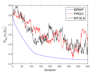
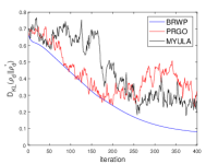
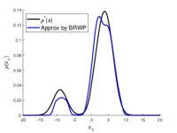
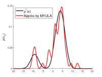
Figure 1. Example 1: Results in $d=20$, step size $h=0.02$, and $50$ particles. From left to right: the decay of KL divergence in the first and the last dimension, density approximated by particles generated by BRWP-splitting and MYULA in the first spatial variable.

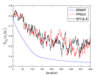
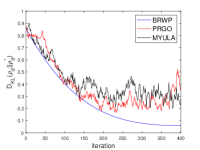
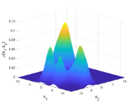
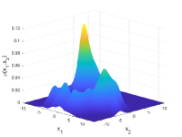
Figure 2. Example 1: Results in $d=50$, step size $h=0.02$, and $100$ particles. From left to right: the decay of KL divergence in the first and the last dimension, density approximated by particles generated by BRWP-splitting and MYULA in the first two spatial variables.

Both experiments in Fig. 1 and Fig. 2 showed that the proposed BRWP-splitting scheme provides a more accurate approximation to the target distribution in terms of KL divergence and the density obtained from kernel density estimation.

5.2. Example 2

The next experiment concerns the Bayesian logistic regression motivated by [12]. The task is to estimate unknown parameter $\theta\in\mathbb{R}^{d}$. Given binary variable (label) $y=\{0,1\}$ under features (covariate) $x\in\mathbb{R}^{n}$, the logistic model for $y$ given $x$ can be modeled as

$$p(y=1|\theta,x)=\frac{\exp(\theta^{T}x)}{1+\exp(\theta^{T}x)}\,,$$ (51)

for some parameter $\theta$ that we try to estimate.

Suppose now we obtain a set of data pairs $\{(x_{i},y_{i})\}_{i=1}^{n}$ where each $y_{i}$ conditioned on $x_{i}$ is drawn from a logistic distribution with parameters $\theta^{*}$. Then using the Bayes rule, we can construct the posterior distribution of parameter $\theta$ in terms of data $\{y_{i}\}$. Denoting $Y=[y_{1},\cdots,y_{n}]$, $X=[x_{1},\cdots,x_{n}]$ and writing $\pi_{0}(x)=\exp(-\lambda\|x\|_{1})$ to be the prior distribution, then the posterior distribution for parameters $\theta$ is computed as

$$p(\theta|y)=p(y|\theta,x)p_{0}(\theta)=\frac{1}{Z}\exp\left(Y^{T}X\theta-\sum_{i=1}^{N}\log(1+\exp(\theta^{T}x_{i}))-\lambda\|\theta\|_{1}\right)\,.$$

For our numerical experiments, $x_{i}$ is normalized where each component is sampled from Rademacher distribution, i.e., which takes the values $\pm 1$ with probability $\frac{1}{2}$. Given $x_{i}$, we then draw $y_{i}$ from the logistic model (51) with $\theta=\theta^{*}$. The parameter $\theta^{*}\in\mathbb{R}^{d}$ contains only $d/4$ non-zero components with value $1$. We examine the performance of the algorithm by computing the $L_{1}$ distance between sample mean $\overline{\theta}$ and the true parameter $\theta^{*}$

$$\frac{1}{d}\|\overline{\theta}-\theta^{*}\|_{1}\,.$$

The regularization parameter is chosen as $\lambda=3d/(2\pi^{2})$, and the results are presented in Fig. 3.

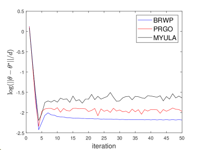
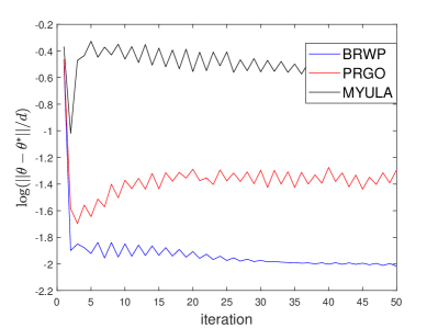
Figure 3. Example 2: Logarithm of relative $L_{1}$ error $\log\left(\|\overline{\theta}-\theta^{*}\|_{1}/d\right)$ in Bayesian logistic regression for 100 particles and $h=0.05$ with $d=20$ (left) and $d=50$ (right).

From Fig. 3, it is clear that the proposed BRWP-splitting method provides a more accurate estimate of the mean parameter in this Bayesian logistic regression.

5.3. Example 3

In this example, we apply the proposed sampling algorithm in image denoising with $L_{1-2}$ regularization as proposed in [37].

The posterior distribution under consideration is

$$\rho^{*}(u)=\frac{1}{Z}\exp\left(-\left(\frac{1}{2}\|Au-y\|_{2}^{2}+\lambda(\|Du\|_{1}-\|Du\|_{2})\right)\right)\,,$$ (52)

the first term in the exponent is a data-fitting term and the second term is the difference between $L_{1}$ and $L_{2}$ norm with the discrete gradient operator defined in section 4 which promotes the sparsity of the image variation. Here, each $u$ corresponds to one single image. To tackle this, the log-density is split as

$$f=\|Au-y\|_{2}^{2}-\lambda\|Du\|_{2}\,,\quad g=\lambda\|Du\|_{1}\,.$$ (53)

To handle the second terms with $L_{1}$-TV norm, we apply the algorithm proposed in Algorithm 2. We consider the case that $A$ is a noisy measurement operator such that

$$A=I+\epsilon\,,$$

where $\epsilon$ is a sparse Gaussian noise with mean $0$, variance $0.1$, that has $3d$ non-zero entries. For the exact image $z_{ex}$, the noisy image $z$ is taken as $Az_{ex}+\eta$ where $\eta$ is a Gaussian noise with mean $0$ and variance $0.2$. The results obtained with $20$ samples and $h=0.1$ are plotted in Fig. 4 and Fig. 5.

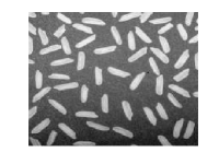
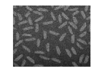
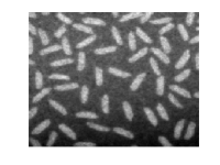
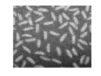
Figure 4. Example 3: Left to right: exact image, noisy image, mean of all samples after 100 iterations by BRWP-splitting and MYULA.

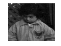
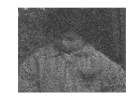
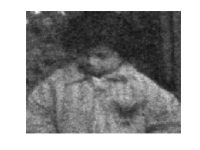
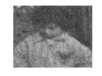
Figure 5. Example 3: Left to right: exact image, noisy image, mean of all samples after 100 iterations by BRWP-splitting and MYULA.

From both Fig. 4 and Fig. 5, the proposed sampling method recovers the original image from noisy data properly with $L_{1-2}$ TV regularization.

5.4. Example 4

In the next example, we examine the application of the proposed sampling algorithm for a compressive sensing application with $L_{1}$ regularization. The target function for this problem is defined as

$$\rho^{*}(x)=\frac{1}{Z}\exp(-\left(\|Ax-z\|_{2}^{2}+\lambda\|x\|_{1}\right))\,,$$ (54)

where $x\in\mathbb{R}^{d}$, $A$ is a $m\times d$ circulant blurring matrix with $m=d/4$.

To quantify the uncertainty in the measurement data, we consider the concept of the highest posterior density (HPD). For a given confidence level $\alpha\in[0,1]$, the HPD region $C_{\alpha}$ is defined as

$$\int_{C_{\alpha}}\rho(x)\,dx=1-\alpha\,,\quad C_{\alpha}:=\{x\in\mathbb{R}^{d}:V(x)\leq\eta_{\alpha}\}\,,$$

where $\eta_{\alpha}$ is a threshold corresponding to the confidence level. The integral can be numerically approximated using samples we get from the BRWP-splitting algorithm. For an arbitrary test image $\tilde{x}$, by comparing $V(\tilde{x})$ with $\eta_{\alpha}$ for various $\alpha$, we can assess the confidence that $\tilde{x}$ belongs to the high-probability region of the posterior distribution. In particular, with the set of particles generated from the BRWP-splitting scheme, the integral is computed numerically as

$$\int_{C_{\alpha}}\rho(x)\,dx\approx\frac{\sum_{j}\mathcal{\chi}_{V(x_{j})<\eta_{\alpha}}}{N}\,,$$

where $N$ is the total number of samples, and $\mathcal{\chi}_{V(x_{j})<\eta_{\alpha}}$ is the indicator function equals to 1 if $V(x_{j})<\eta_{\alpha}$ and 0 otherwise.

We test the algorithm on a brain MRI image of size $d=128^{2}$. The measurement model is assumed to be $Ax+\epsilon$, where $\epsilon$ represents Gaussian noise with mean 0 and variance 0.2. The reconstruction is estimated using a step size $h=0.02$, with 100 samples and 100 iterations. Additionally, we compute the HPD region threshold and plot the graph of $\eta_{\alpha}$ versus $\alpha$, which is estimated using 1000 samples.

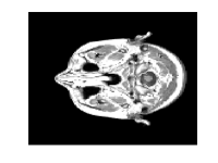
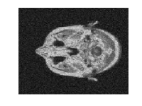
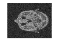
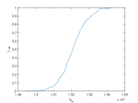
Figure 6. Example 4: From left to right: exact MRI image, reconstructed MRI image with BRWP-splitting, reconstructed MRI image with MYULA, HDP region thresholds $\eta_{\alpha}$.

From Fig.6, we observe that the proposed algorithm yields a better reconstruction compared with MYULA. Furthermore, the sampling approach allows us to compute the HPD region threshold, facilitating practical Bayesian inference analysis.

5.5. Example 5

In this example, we apply the proposed method to Bayesian neural network training. Specifically, the likelihood function is modeled as an isotropic Gaussian, and the prior distribution is Laplace prior. We consider a two-layer neural network, where each layer consists of 50 hidden units with a ReLU activation function. For each dataset, $90\%$ of the data is used for training, while the remaining $10\%$ is reserved for testing. Each algorithm is simulated using 200 particles over 500 iterations.

We compare the BRWP-splitting against MYULA, the original BRWP (non-splitting, without proximal computation), and SVGD (Stein variational gradient descent). The step size for each method is selected via grid search to achieve the best performance, and it remains consistent across all experiments.

Dataset	BRWP-splitting	BRWP	MYULA	SVGD
Boston	$\mathbf{3.78_{\pm 1.93\times 10^{-1}}}$	$4.27_{\pm 2.09\times 10^{-2}}$	$6.29_{\pm 6.00\times 10^{-3}}$	$4.05_{\pm 6.93\times 10^{-2}}$
Wine	$\mathbf{0.53_{\pm 2.54\times 10^{-1}}}$	$0.61_{\pm 2.47\times 10^{-1}}$	$0.72_{\pm 1.13\times 10^{-1}}$	$0.54_{\pm 3.64\times 10^{-1}}$
Concrete	$\mathbf{3.25_{\pm 1.37\times 10^{-1}}}$	$4.11_{\pm 1.02\times 10^{-1}}$	$4.71_{\pm 3.14\times 10^{-1}}$	$3.32_{\pm 1.47\times 10^{-1}}$
Kin8nm	${0.093_{\pm 7.99\times 10^{-4}}}$	$0.135_{\pm 2.15\times 10^{-3}}$	$0.294_{\pm 1.56\times 10^{-3}}$	$\mathbf{0.092_{\pm 7.93\times 10^{-4}}}$
Power	$\mathbf{4.13_{\pm 3.21\times 10^{-2}}}$	$5.25_{\pm 8.42\times 10^{-2}}$	$8.49_{\pm 2.87\times 10^{-1}}$	$4.15_{\pm 1.63\times 10^{-2}}$
Protein	$\mathbf{4.23_{\pm 2.17\times 10^{-2}}}$	$4.74_{\pm 4.32\times 10^{-2}}$	$5.12_{\pm 7.32\times 10^{-2}}$	$4.61_{\pm 1.93\times 10^{-2}}$
Energy	$\mathbf{1.54_{\pm 2.37\times 10^{-2}}}$	$3.06_{\pm 6.06\times 10^{-2}}$	$4.52_{\pm 2.42}$	$2.00_{\pm 4.13\times 10^{-2}}$

Table 1. Example 5: Root-mean-square error for different datasets in Bayesian neural network training with $\lambda=1/d$.

From Table 1, we observe that, for most datasets tested, the proposed BRWP-splitting approach achieves a lower root-mean-square error compared to the other methods.

6. Discussions

In this work, we propose a sampling algorithm based on splitting methods and regularized Wasserstein proximal operators for sampling from nonsmooth distributions. When the log-density of the prior distribution is the $L_{1}$ norm, the scheme is formulated as an interacting particle system incorporating shrinkage operators and the softmax function. The resulting iterative sampling scheme is simple to implement and naturally promotes sparsity. Theoretical convergence of the proposed scheme is established under suitable conditions and the algorithm’s efficiency is demonstrated through extensive numerical experiments.

For future directions, we aim to extend our theoretical analysis to investigate the algorithm’s convergence in the finite-particle approximation and explore its applicability beyond log-concave sampling. On the computational side, we seek to enhance efficiency through GPU-based parallel implementations and examine the impact of different kernel choices on the performance. Additionally, as discussed in Section 2.4, regularized Wasserstein proximal operators share a close structural connection with transformer architectures, motivating our interest in analyzing the self-attention mechanism through the lens of interacting particle systems. More importantly, building on the proposed algorithm, we plan to develop tailored transformer models for learning sparse data distributions, which are only known by samples.

Acknowledgement: F. Han’s work is partially supported by AFOSR YIP award No. FA9550 -23-10087. F. Han and S. Osher’s work is partially supported by ONR N00014-20-1-2787, NSF-2208272, STROBE NSF-1554564, and NSF 2345256. W. Li’s work is supported by AFOSR YIP award No. FA9550-23-10087, NSF RTG: 2038080, and NSF DMS-2245097.

Appendix A Derivation in Section 2

Proof of proposition 1.

For the case $\rho_{k}$ is approximated with Gaussian kernel, writing $x_{\ell}$ as the $\ell$-th component of $x\in\mathbb{R}^{d}$, we note (14) becomes

$$K_{g}^{h}\rho_{k}(x) =\frac{1}{N(2\pi\sigma^{2})^{d/2}}\exp\left(-\frac{\beta}{2}\lambda\|x\|_{1}\right)\cdot$$

$$\sum_{j=1}^{N}\prod_{\ell=1}^{d}\int_{\mathbb{R}}\exp\left[-\frac{\beta}{2}\left(\frac{(x_{\ell}-y_{\ell})^{2}-(y_{\ell}-S_{\lambda h}(y_{\ell}))^{2}}{2h}-\lambda|S_{\lambda h}(y_{\ell})|\right)-\frac{(y_{\ell}-x_{j,\ell})^{2}}{2\sigma^{2}}\right]dy_{\ell}\,.$$

Hence, obtaining the closed-form formula reduces to evaluating a one-dimensional exponential integral. This integral can be decomposed into three parts: $[\lambda h,\infty)$, $(-\lambda h,\lambda h)$, and $(-\infty,-\lambda h]$, following the definition of the shrinking operator $S_{\lambda h}(y)$. Defining $c=2h/(\sigma^{2}\beta)$, denoting $\psi(x,x_{j})=\exp\left(-\frac{\beta}{2}\left(\frac{x^{2}+cx_{j}^{2}}{2h}\right)\right)$ to simplify notation, and omitting the index $\ell$ for simplicity, the integral over $[\lambda h,\infty)$ is given by

$$\psi(x,x_{j})\int_{\lambda h}^{\infty}\exp\left(-\frac{\beta}{4h}\left[(1+c)y^{2}-2y(x+cx_{j}+\lambda h)\right]\right)dy\exp\left(-\frac{\beta\lambda^{2}h}{4}\right)$$

$$= \psi(x,x_{j})\sqrt{\frac{4h}{\beta(1+c)}}$$

$$\int_{\sqrt{\frac{\beta(1+c)}{4h}}\left[\lambda h-\frac{x+cx_{j}+\lambda h}{1+c}\right]}^{\infty}\exp(-y^{2})dy\exp\left(-\frac{\beta}{4h}\left(\lambda^{2}h^{2}-\frac{(x+cx_{j}+\lambda h)^{2}}{1+c}\right)\right)\,.$$

Similarly, the integral on $(-\infty,-\lambda h]$ will be

$$\psi(x,x_{j})\int_{-\infty}^{-\lambda h}\exp\left(-\frac{\beta}{4h}\left[(1+c)y^{2}-2y(x+cx_{j}-\lambda h)\right]\right)dy\exp\left(-\frac{\beta\lambda^{2}h}{4}\right)$$

$$= \psi(x,x_{j})\sqrt{\frac{4h}{\beta(1+c)}}$$

$$\int^{\sqrt{\frac{\beta(1+c)}{4h}}\left[-\lambda h-\frac{x+cx_{j}-\lambda h}{(1+c)}\right]}_{-\infty}\exp(-y^{2})dy\exp\left(-\frac{\beta}{4h}\left(\lambda^{2}h^{2}-\frac{(x+cx_{j}-\lambda h)^{2}}{1+c}\right)\right)\,.$$

Finally the integral on $[-\lambda h,\lambda h]$ can be computed as

$$\psi(x,x_{j})\int_{-\lambda h}^{\lambda h}\exp\left(-\frac{\beta}{4h}\left(cy^{2}-2y(x+cx_{j})\right)\right)dy$$

$$= \psi(x,x_{j})\int_{-\lambda h}^{\lambda h}\exp\left(-\frac{c\beta}{4h}\left[y-\frac{(x+cx_{j})}{c}\right]^{2}\right)dy\exp\left(\frac{\beta}{4h}\frac{(x+cx_{j})^{2}}{c}\right)$$

$$= \psi(x,x_{j})\sqrt{\frac{4h}{c\beta}}\int_{\sqrt{\frac{c\beta}{4h}}\left[-\lambda h-\frac{(x+cx_{j})}{c}\right]}^{\sqrt{\frac{c\beta}{4h}}\left[\lambda h-\frac{(x+cx_{j})}{c}\right]}\exp(-y^{2})dy\exp\left(\frac{\beta}{4h}\frac{(x+cx_{j})^{2}}{c}\right)\,.$$

Next, to compute the score function, we need to evaluate $\nabla K_{g}^{h}\rho_{k}$ on each sub-integral. For the integral on $[\lambda h,\infty)$, omitting the $\psi$ term, direct computation implies the following

$$\nabla\left\{\sqrt{\frac{4h}{\beta(1+c)}}\int_{\sqrt{\frac{\beta(1+c)}{4h}}\left[\lambda h-\frac{x+cx_{j}+\lambda h}{1+c}\right]}^{\infty}\exp(-y^{2})dy\exp\left(-\frac{\beta}{4h}\left(\lambda^{2}h^{2}-\frac{(x+cx_{j}+\lambda h)^{2}}{1+c}\right)\right)\right\}$$

$$= \Bigg{\{}\sqrt{\frac{\beta}{h(1+c)}}(x+cx_{j}+\lambda h)\int_{\sqrt{\frac{\beta(1+c)}{4h}}\left[\lambda h-\frac{x+cx_{j}+\lambda h}{1+c}\right]}^{\infty}\exp(-y^{2})dy$$

$$+\exp\left[-\frac{\beta(1+c)}{4h}\left(\lambda h-\frac{x+cx_{j}+\lambda h}{1+c}\right)^{2}\right]\Bigg{\}}\cdot\frac{\exp\left(-\frac{\beta}{4h}\left(\lambda^{2}h^{2}-\frac{(x+cx_{j}+\lambda h)^{2}}{1+c}\right)\right)}{1+c}\,.$$

The gradient for the integral on $(-\infty,-\lambda h]$ can be evaluated similarly to the above by replacing $x+cx_{j}+\lambda h$ with $x+c_{j}-\lambda h$ and change of signs. Finally, the gradient for the integral on $(-\lambda h,\lambda h)$ can be evaluated as

$$\nabla\left\{\sqrt{\frac{4h}{c\beta}}\int_{\sqrt{\frac{c\beta}{4h}}\left[-\lambda h-\frac{(x+cx_{j})}{c}\right]}^{\sqrt{\frac{c\beta}{4h}}\left[\lambda h-\frac{(x+cx_{j})}{c}\right]}\exp(-y^{2})dy\exp\left(\frac{\beta}{4h}\frac{(x+cx_{j})^{2}}{c}\right)\right\}$$

$$= \exp\left(\frac{\beta}{4h}\frac{(x+cx_{j})^{2}}{c}\right)\cdot\Bigg{\{}\sqrt{\frac{4h}{c\beta}}\frac{\beta}{2h}\frac{(x+cx_{j})}{c}\int_{\sqrt{\frac{c\beta}{4h}}\left[-\lambda h-\frac{(x+cx_{j})}{c}\right]}^{\sqrt{\frac{c\beta}{4h}}\left[\lambda h-\frac{(x+cx_{j})}{c}\right]}\exp(-y^{2})dy$$

$$-\frac{1}{c}\left[\exp\left(-\frac{c\beta}{4h}\left(\lambda h-\frac{x+cx_{j}}{c}\right)^{2}\right)-\exp\left(-\frac{c\beta}{4h}\left(-\lambda h-\frac{x+cx_{j}}{c}\right)^{2}\right)\right]\Bigg{\}}\,.$$

Combining the above gives the desired result. ∎

Proof of proposition 2.

For the sum of $A_{i,j}$ defined in (25), we have

$$\sum_{j=1}^{N^{d}}A_{i,j}=\sum_{j=1}^{N^{d}}\exp\left(-\frac{\beta}{2}\left(\frac{\|x^{k}_{i}-\tilde{x}^{k}_{j}\|_{2}^{2}}{2h}\right)\right)\exp\left(\frac{\beta}{2}\left(\frac{\|S_{\lambda h}(\tilde{x}^{k}_{j})-\tilde{x}^{k}_{j}\|_{2}^{2}}{2h}+\lambda\|S_{\lambda h}(\tilde{x}^{k}_{j})\|_{1}\right)\right)$$

$$= \sum_{j=1}^{N^{d}}\prod_{\ell=1}^{d}\exp\left(-\frac{\beta}{2}\left(\frac{(x^{k}_{i,\ell}-\tilde{x}^{k}_{j,\ell})^{2}}{2h}\right)\right)\exp\left(\frac{\beta}{2}\left(\frac{(S_{\lambda h}(\tilde{x}^{k}_{j,\ell})-\tilde{x}^{k}_{j,\ell})^{2}}{2h}+\lambda|S_{\lambda h}(\tilde{x}^{k}_{j,\ell})|\right)\right)$$

$$= \sum_{j_{1}=1}^{N}\cdots\sum_{j_{d-1}=1}^{N}\prod_{\ell=1}^{d-1}\sum_{j_{d}=1}^{N}\exp\left(-\frac{\beta}{2}\left(\frac{(x^{k}_{i,\ell}-x^{k}_{j_{\ell},\ell}}{2h}\right)\right)\cdot$$

$$\hskip 170.71652pt\exp\left(\frac{\beta}{2}\left(\frac{(S_{\lambda h}(x^{k}_{j_{\ell},\ell})-x^{k}_{j_{\ell},\ell})^{2}}{2h}+\lambda|S_{\lambda h}(x^{k}_{j_{\ell},\ell})|\right)\right)\,.$$

Then, we can rearrange the terms to get

$$\sum_{j=1}^{N^{d}}A_{i,j}=\prod_{\ell=1}^{d}\sum_{j=1}^{N}\exp\left(-\frac{\beta}{2}\left(\frac{(x^{k}_{i,\ell}-x^{k}_{j,\ell})^{2}}{2h}\right)\right)\exp\left(\frac{\beta}{2}\left(\frac{(S_{\lambda h}(x^{k}_{j,\ell})-x^{k}_{j,\ell})^{2}}{2h}+\lambda|S_{\lambda h}(x^{k}_{j,\ell})|\right)\right)\,,$$

which is the desired formula in the proposition. ∎

Appendix B Postponed Proof in Section 3

Proof of Lemma 4.

The proximal term in (4) can be rewritten using the property of the proximal operator as

$$\frac{x-\text{prox}_{g}^{h}(x)}{h}=\nabla g_{h}(x)\,.$$

Thus, the formula (4) is equivalent to

$$K_{g}^{h}\rho_{k+\frac{1}{2}}(x)$$ (55)

$$= \frac{\nabla\exp\left(-\frac{\beta}{2}g_{h}(x)\right)\int\exp\left[-\frac{\beta}{4h}\left(\|x-y\|_{2}^{2}-\|y-\text{prox}_{g}^{h}(y)\|_{2}^{2}-hg(\text{prox}_{g}^{h}(y))\right)\right]\rho_{k+\frac{1}{2}}(y)dy}{\exp\left(-\frac{\beta}{2}g_{h}(x)\right)\int\exp\left[-\frac{\beta}{4h}\left(\|x-y\|_{2}^{2}-\|y-\text{prox}_{g}^{h}(y)\|_{2}^{2}-hg(\text{prox}_{g}^{h}(y))\right)\right]\rho_{k+\frac{1}{2}}(y)dy}\,.$$

Since $g_{h}$ is gradient-Lipschitz, its Hessian exists and is bounded almost everywhere. Additionally, as $g_{h}(x)=g(x)+\mathcal{O}(h)$ by Lemma 3, we can substitute $g_{h}$ for $g$ in (55), introducing an additional error term of $\mathcal{O}(h)$ in the exponent. Moreover, since the dominating term in the exponent is of order $1/h$, the error resulting from replacing $g$ with $g_{h}$ will be of order $\mathcal{O}(h^{2})$ after taking the quotient.

Applying the Laplace method (see [17] for details), we obtain

$$\int_{\mathbb{R}^{d}}\exp\left(-\frac{\beta}{2}\left(g_{h}(z)+\frac{\|y-z\|_{2}^{2}}{2h}\right)\right)dz$$ (56)

$$= C\frac{\exp\left(-\frac{\beta}{2}\left(g_{h}(\text{prox}^{h}_{g_{h}}(y))+\frac{\|\text{prox}_{g_{h}}^{h}(y)-y\|_{2}^{2}}{2h}\right)\right)}{1+\frac{h}{2}\Delta g_{h}(\text{prox}_{g_{h}}^{h}(y))}+\mathcal{O}(h^{2})\,,$$

for constant $C=(2\pi h)^{d/2}$ almost everywhere. We note that the Laplacian term in the denominator will be concealed after taking the quotient in (55).

Substituting (56) into (55) leads to

$$K_{g}^{h}\rho_{k+\frac{1}{2}}(x)=\int_{\mathbb{R}^{d}}\frac{\exp\big{[}-\frac{\beta}{2}\big{(}g_{h}(x)+\frac{||x-y||_{2}^{2}}{2h}\big{)}\big{]}}{\int_{\mathbb{R}^{d}}\exp\big{[}-\frac{\beta}{2}\big{(}g_{h}(z)+\frac{||z-y||_{2}^{2}}{2h}\big{)}\big{]}dz}\rho_{k+\frac{1}{2}}(y)dy+\mathcal{O}(h^{2})\,.$$ (57)

Thus, it remains to verify that $K_{g}^{h}\rho_{k+\frac{1}{2}}$ approximates the evolution of the Fokker–Planck equation with drift term $\nabla g_{h}$ from $t_{k}$ to $t_{k}+h$. This follows from the assumption on $\rho_{k+\frac{1}{2}}$, $g_{h}$, and Theorem 4 in [17]. ∎

Our proof of the convergence of Rényi divergence will rely on the interpolation argument by considering the continuity equation of (37) in time $t\in[kh,(k+1)h]$. The particle at time $t$ is written as

$$x_{t}-x_{kh}$$ (58)

$$= -(t-kh)\left[\nabla f(x_{kh})+\nabla g_{h}(x_{kh}-h\nabla f(x_{kh}))+\beta^{-1}\nabla\log K_{g}^{(t-kh)}\rho_{k+\frac{1}{2}}(x_{kh}-h\nabla f(x_{kh}))\right]$$

$$= -(t-kh)\left[\nabla f(x_{t})+\nabla g_{h}(x_{t})+\beta^{-1}\nabla\log\rho_{t}(x_{t})+\Lambda(x_{t},x_{kh})\right]\,,$$

where

$$\Lambda(x_{t},x_{kh}):= -\beta^{-1}\nabla\log\frac{\rho_{t}}{\rho_{h}^{*}}(x_{t})+\beta^{-1}\nabla\log\frac{\rho_{t}}{\rho_{h}^{*}}(x_{kh}-h\nabla f(x_{kh}))$$

$$+\nabla f(x_{kh})-\nabla f(x_{kh}-h\nabla f(x_{kh}))$$

$$-\beta^{-1}\nabla\log\rho_{t}(x_{kh}-h\nabla f(x_{kh}))+\beta^{-1}\nabla\log K_{g}^{t-kh}\rho_{k+\frac{1}{2}}(x_{kh}-h\nabla f(x_{kh}))\,.$$

We note that when $t=(k+1)h$, we have $x_{t}=x^{k+1}$, i.e., the location of the particle in the next time step.

Then the Fokker Planck equation corresponds to (58) for $t\in[kh,(k+1)h]$ will be

$$\frac{\partial\rho_{t}}{\partial t}(x_{t})=\beta^{-1}\nabla\cdot\left(\rho_{t}(x_{t})\nabla\log\frac{\rho_{t}}{\rho_{h}^{*}}(x_{t})\right)+\nabla\cdot\left(\rho_{t}(x_{t})\Lambda(x_{t},x_{kh})\right).$$ (59)

We now state the following lemma on the time derivative of Rényi divergence along (59).

Lemma 7.

For $t\in[kh,(k+1)h]$, the time derivative of the Rényi divergence between $\rho_{t}$ along (59) and $\rho_{h}^{*}$ satisfies

$$\frac{\partial}{\partial t}R_{q}(\rho_{t}\|\rho_{h}^{*})\leq-\frac{q}{2}\frac{G_{q}(\rho_{t}\|\rho_{h}^{*})}{F_{q}(\rho_{t}\|\rho_{h}^{*})}+\frac{q}{2F_{q}(\rho_{t}\|\rho_{h}^{*})}\int_{\mathbb{R}^{d}}\|\Lambda(x_{t},x_{kh})\|_{2}^{2}\left(\frac{\rho_{t}}{\rho_{h}^{*}}\right)^{q}\rho_{h}^{*}\,dx_{t}\,.$$ (60)

Proof.

By the definition of the Rényi divergence, we have

$$\frac{\partial}{\partial t}R_{q}(\rho_{t}\|\rho_{h}^{*})=\frac{q}{q-1}\frac{\int_{\mathbb{R}^{d}}\left(\frac{\rho_{t}}{\rho_{h}^{*}}\right)^{q-1}\partial_{t}\rho_{t}\,dx_{t}}{F_{q}(\rho_{t}\|\rho_{h}^{*})}$$

$$= \frac{q}{(q-1)F_{q}(\rho_{t}\|\rho_{h}^{*})}\int_{\mathbb{R}^{d}}\left(\frac{\rho_{t}}{\rho_{h}^{*}}\right)^{q-1}\nabla\cdot\left[\left(\rho_{t}\nabla\log\frac{\rho_{t}}{\rho_{h}^{*}}\right)+\Lambda(x_{t},x_{kh})\rho_{t}\right]dx_{t}$$

$$= -\frac{q}{F_{q}(\rho_{t}\|\rho_{h}^{*})}\int_{\mathbb{R}^{d}}\left(\frac{\rho_{t}}{\rho_{h}^{*}}\right)^{q-2}\nabla\frac{\rho_{t}}{\rho_{h}^{*}}\cdot\left[\left(\rho_{t}\nabla\log\frac{\rho_{t}}{\rho_{h}^{*}}\right)+\Lambda(x_{t},x_{kh})\rho_{t}\right]dx_{t}$$

$$= -\frac{q}{F_{q}(\rho_{t}\|\rho_{h}^{*})}\left[\int_{\mathbb{R}^{d}}\left\|\nabla\frac{\rho_{t}}{\rho_{h}^{*}}\right\|_{2}^{2}\left(\frac{\rho_{t}}{\rho_{h}^{*}}\right)^{q-2}\rho_{h}^{*}\,dx_{t}+\int_{\mathbb{R}^{d}}\left(\frac{\rho_{t}}{\rho_{h}^{*}}\right)^{q-1}\nabla\frac{\rho_{t}}{\rho_{h}^{*}}\cdot\Lambda(x_{t},x_{kh})\rho_{h}^{*}\,dx_{t}\right]\,.$$

The first term is precisely the Rényi information term defined in (38), and the second term represents the discretization error, which we need to bound. The second term can be further simplified as follows:

$$\int_{\mathbb{R}^{d}}\left(\frac{\rho_{t}}{\rho_{h}^{*}}\right)^{q-1}\nabla\frac{\rho_{t}}{\rho_{h}^{*}}\cdot\Lambda(x_{t},x_{kh})\rho_{h}^{*}\,dx_{t}=\int_{\mathbb{R}^{d}}\nabla\frac{\rho_{t}}{\rho_{h}^{*}}\cdot\left[\Lambda(x_{t},x_{kh})\frac{\rho_{t}}{\rho_{h}^{*}}\right]\left(\frac{\rho_{t}}{\rho_{h}^{*}}\right)^{q-2}\rho_{h}^{*}\,dx_{t}$$

$$\geq -\frac{1}{2}\int_{\mathbb{R}^{d}}\left\|\nabla\frac{\rho_{t}}{\rho_{h}^{*}}\right\|_{2}^{2}\left(\frac{\rho_{t}}{\rho_{h}^{*}}\right)^{q-2}\rho_{h}^{*}\,dx_{t}-\frac{1}{2}\int_{\mathbb{R}^{d}}\|\Lambda(x_{t},x_{kh})\|_{2}^{2}\left(\frac{\rho_{t}}{\rho_{h}^{*}}\right)^{q}\rho_{h}^{*}\,dx_{t}\,.$$

The final result is obtained by combining the above relations. ∎

Next, we will bound the discretization error using the Lipschitz continuity of the score function and $(f+g_{h})$.

Lemma 8.

The discretization error term $\Lambda(x_{t},x_{kh})$ satisfies

$$\int_{\mathbb{R}^{d}}\|\Lambda(x_{t},x_{kh})\|_{2}^{2}\left(\frac{\rho_{t}}{\rho_{h}^{*}}\right)^{q}\rho_{h}^{*}dx_{t}\leq\frac{2L^{2}h^{2}}{(1-hL)^{2}}G_{q}(\rho_{t}\|\rho_{h}^{*})+2L_{f}^{2}(L+L_{f})^{2}h^{2}dF_{q}(\rho_{t}\|\rho_{h}^{*})+\mathcal{O}(h^{3})\,,$$ (61)

where $L=L_{f}+L_{g_{h}}+L_{\rho}$.

Proof.

Firstly, using the gradient Lipschitz condition on $f$, $g_{h}$, and $\log\rho_{t}$, and also the approximation result in Lemma 4, we can bound the discretization error as

$$\|\Lambda(x_{t},x_{kh})\|_{2}\leq \,L\|x_{t}-x_{kh}+h\nabla f(x_{kh})\|_{2}+L_{f}h\|\nabla f(x_{kh})\|_{2}+\mathcal{O}(h^{2})$$

$$\leq \,L\|x_{t}-x_{kh}\|_{2}+(L+L_{f})h\|\nabla f(x_{kh})\|_{2}+\mathcal{O}(h^{2})$$ (62)

$$\leq \,L\|x_{t}-x_{kh}\|_{2}+h(L+L_{f})L_{f}\sqrt{d}+\mathcal{O}(h^{2})\,.$$

For the first term of (B), by the formula for $x_{t}$ in (58), we obtain

$$\left\|x_{t}-x_{kh}\right\|_{2}\leq \,h\left\|\nabla\log\frac{\rho_{t}}{\rho_{h}^{*}}(x_{kh})\right\|_{2}+\mathcal{O}(h^{2})$$

$$\leq \,h\left\|\nabla\log\frac{\rho_{t}}{\rho_{h}^{*}}(x_{t})\right\|_{2}+h\left\|\nabla\log\frac{\rho_{t}}{\rho_{h}^{*}}(x_{t})-\nabla\log\frac{\rho_{t}}{\rho_{h}^{*}}(x_{kh})\right\|_{2}+\mathcal{O}(h^{2})$$

$$\leq \,h\left\|\nabla\log\frac{\rho_{t}}{\rho_{h}^{*}}(x_{t})\right\|_{2}+Lh\left\|x_{t}-x_{kh}\right\|_{2}+\mathcal{O}(h^{2})\,.$$

The above leads to

$$\|x_{t}-x_{kh}\|_{2}\leq\frac{h}{1-hL}\left\|\nabla\log\frac{\rho_{t}}{\rho_{h}^{*}}(x_{t})\right\|+\mathcal{O}(h^{2})\,.$$

Substituting this back into $\Lambda(x_{t},x_{kh})$, we get

$$\int_{\mathbb{R}^{d}}\|\Lambda(x_{t},x_{kh})\|_{2}^{2}\left(\frac{\rho_{t}}{\rho_{h}^{*}}\right)^{q}\rho_{h}^{*}dx_{t}$$

$$\leq \,\frac{2L^{2}h^{2}}{(1-hL)^{2}}\int_{\mathbb{R}^{d}}\left\|\nabla\log\frac{\rho_{t}}{\rho_{h}^{*}}\right\|_{2}^{2}\left(\frac{\rho_{t}}{\rho_{h}^{*}}\right)^{q}\rho_{h}^{*}dx_{t}+2L_{f}^{2}(L+L_{f})^{2}h^{2}d\int_{\mathbb{R}^{d}}\left(\frac{\rho_{t}}{\rho_{h}^{*}}\right)^{q}\rho_{h}^{*}dx_{t}+\mathcal{O}(h^{3})$$

$$= \,\frac{2L^{2}h^{2}}{(1-hL)^{2}}G_{q}(\rho_{t}\|\rho_{h}^{*})+2L_{f}^{2}(L+L_{f})^{2}h^{2}dF_{q}(\rho_{t}\|\rho_{h}^{*})+\mathcal{O}(h^{3})\,.$$

∎

Next, we are ready to prove Theorem 6.

Proof of Theorem 6 part (1).

By combining Lemma 7 and 8, we have

$$\frac{\partial}{\partial t}R_{q}(\rho_{t}\|\rho_{h}^{*})=\,-\frac{q}{2}\frac{G_{q}(\rho_{t}\|\rho_{h}^{*})}{F_{q}(\rho_{t}\|\rho_{h}^{*})}+\frac{q}{2F_{q}(\rho_{t}\|\rho_{h}^{*})}\int_{\mathbb{R}^{d}}\|\Lambda(x_{t},x_{kh})\|_{2}^{2}\left(\frac{\rho_{t}}{\rho_{h}^{*}}\right)^{q}\rho_{h}^{*}dx_{t}$$

$$\leq \,\frac{q}{2}\left(-1+\frac{2L^{2}h^{2}}{(1-hL)^{2}}\right)\frac{G_{q}(\rho_{t}\|\rho_{h}^{*})}{F_{q}(\rho_{t}\|\rho_{h}^{*})}+qL_{f}^{2}(L+L_{f})^{2}h^{2}d+\mathcal{O}(h^{3})\,.$$

Using the result in Lemma 5, i.e., when $\rho_{h}^{*}$ satisfies the Poincaré inequality with constant $\alpha_{d}$, we have

$$\frac{G_{q}(\rho\|\rho_{h}^{*})}{F_{q}(\rho\|\rho_{h}^{*})}\geq\frac{4\alpha_{d}}{q^{2}}\left(1-\exp(-R_{q}(\rho\|\rho_{h}^{*}))\right)\,.$$

Hence, we arrive at

$$\frac{\partial}{\partial t}R_{q}(\rho_{t}\|\rho_{h}^{*})\leq\frac{2\alpha_{d}}{q}\left(1-\exp(-R_{q}(\rho_{t}\|\rho_{h}^{*}))\right)\left(-1+\frac{2L^{2}h^{2}}{(1-hL)^{2}}\right)+qL^{2}(L+L_{f})^{2}h^{2}d+\mathcal{O}(h^{3})\,,$$

when $h\leq(\sqrt{2}-1)/L$.

Writing $\rho_{k}=\rho_{kh}$. Then when $R_{q}(\rho_{0}\|\rho_{h}^{*})\geq 1$, it follows $1-\exp(-R_{q}(\rho_{k}\|\rho_{h}^{*}))\geq\frac{1}{2}$. In this case, we can derive the linear convergence given by

$$R_{q}(\rho_{k}\|\rho_{h}^{*})\leq R_{q}(\rho_{0}\|\rho_{h}^{*})-kh\left(\frac{\alpha_{d}}{q}\left(1-\frac{2L^{2}h^{2}}{(1-hL)^{2}}\right)-qL^{2}(L+L_{f})^{2}h^{2}d\right)+\mathcal{O}(h^{3})\,.$$

For the case $R_{q}(\rho_{0}\|\rho_{h}^{*})<1$, we note that

$$1-\exp(-R_{q}(\rho_{0}\|\rho_{h}^{*}))\geq R_{q}(\rho_{0}\|\rho_{h}^{*})-\frac{R_{q}(\rho_{0}\|\rho_{h}^{*})^{2}}{2}\geq\frac{1}{2}R_{q}(\rho_{0}\|\rho_{h}^{*})\,.$$

In this scenario, by integration with respect to $t$ from $0$ to $kh$, we have

$$R_{q}(\rho_{k}\|\rho_{h}^{*})\leq R_{q}(\rho_{0}\|\rho_{h}^{*})\exp\left[-kh\frac{\alpha_{d}}{q}\left(1-\frac{2L^{2}h^{2}}{(1-hL)^{2}}\right)\right]+\frac{q^{2}L^{2}(L+L_{f})^{2}h^{2}d}{\alpha_{d}}+\mathcal{O}(h^{3})\,.$$

∎

Proof of Theorem 6 part (2).

The bound of Rényi divergence between $\rho^{*}$ and $\rho_{h}^{*}$ can be derived using approximation results (b) in Lemma 3 and Taylor expansion of $\log$ function which lead to

$$R_{q}(\rho^{*}\|\rho_{h}^{*})=\frac{1}{q-1}\log\left(\int_{\mathbb{R}^{d}}\left(\frac{\rho^{*}}{\rho_{h}^{*}}\right)^{q}\rho_{h}^{*}\,dx\right)\leq\frac{qL_{g}^{2}h}{q-1}+\mathcal{O}(h^{2})\,.$$

Additionally, we recall the following decomposition theorem for Rényi divergence

$$R_{q}(\rho_{k}\|\rho^{*})\leq\left(\frac{q-\frac{1}{2}}{q-1}\right)R_{2q}(\rho^{*}\|\rho_{h}^{*})+R_{2q-1}(\rho_{k}\|\rho_{h}^{*})\,.$$

Plug in the above two relations into part (1) of Theorem 6, and the desired result can be proved. ∎

Appendix C Details about Numerical Experiments

Evaluation of marginal distribution in Example 1. We can integrate the mixture of Gaussian and Laplace models exactly. If $\Sigma_{i}^{-1}=1/(2\sigma^{2})I_{d}$, the integral is given by

$$\int_{\mathbb{R}^{d}}\rho^{*}(x)\,dx$$

$$= \sum_{n=1}^{N}\prod_{j=1}^{d}\int_{\mathbb{R}}\exp\left(-\frac{(x_{j}-y_{n,j})^{2}}{2\sigma_{n}^{2}}-\lambda|x_{j}|\right)dx_{j}$$

$$= \sum_{n=1}^{N}\prod_{j=1}^{d}\left[\int_{-(y_{n,j}-\lambda\sigma_{n}^{2})}^{\infty}\exp\left(-\frac{z_{j}^{2}}{2\sigma_{n}^{2}}\right)dz_{j}\exp\left(-\frac{y_{n,j}^{2}-(y_{n,j}-\lambda\sigma_{n}^{2})^{2}}{2\sigma_{n}^{2}}\right)\right.$$

$$\quad+\left.\int_{-\infty}^{-(y_{n,j}+\lambda\sigma_{n}^{2})}\exp\left(-\frac{z_{j}^{2}}{2\sigma_{n}^{2}}\right)dz_{j}\exp\left(-\frac{y_{n,j}^{2}-(y_{n,j}+\lambda\sigma_{n}^{2})^{2}}{2\sigma_{n}^{2}}\right)\right]$$

$$= \frac{1}{(\sqrt{2}\sigma_{n})^{d}}\sum_{n=1}^{N}\prod_{j=1}^{d}\left[\int_{-\frac{(y_{n,j}-\lambda\sigma_{n}^{2})}{\sqrt{2}\sigma_{n}}}^{\infty}\exp\left(-z_{j}^{2}\right)dz_{j}\exp\left(-\frac{y_{n,j}^{2}-(y_{n,j}-\lambda\sigma_{n}^{2})^{2}}{2\sigma_{n}^{2}}\right)\right.$$

$$\quad+\left.\int_{-\infty}^{-\frac{(y_{n,j}+\lambda\sigma_{n}^{2})}{\sqrt{2}\sigma_{n}}}\exp\left(-z_{j}^{2}\right)dz_{j}\exp\left(-\frac{y_{n,j}^{2}-(y_{n,j}+\lambda\sigma_{n}^{2})^{2}}{2\sigma_{n}^{2}}\right)\right]\,.$$

The above computation provides the normalization constant $Z$. By replacing the integration over $\mathbb{R}^{d}$ with an integration over $\mathbb{R}^{d-1}$, we obtain the formula for the marginal distribution $\rho_{1}^{*}$.

References

• [1] L. Ambrosio, N. Gigli, and G. Savaré. Gradient flows: in metric spaces and in the space of probability measures. Springer Science & Business Media, 2008.
• [2] M. Benko, I. Chlebicka, J. Endal, and B. Miasojedow. Langevin Monete Carlo beyond lipschitz gradient continuity. arXiv preprint arXiv:2412.09698, 2024.
• [3] E. Bernton. Langevin Monete Carlo and JKO splitting. In Conference on Learning Theory, pages 1777–1798. PMLR, 2018.
• [4] M. Burger, M. J. Ehrhardt, L. Kuger, and L. Weigand. Analysis of primal-dual Langevin algorithms, 2024.
• [5] J. A. Carrillo, F. Hoffmann, A. M. Stuart, and U. Vaes. Consensus-based sampling. Studies in Applied Mathematics, 148(3):1069–1140, 2022.
• [6] V. Castin, P. Ablin, J. A. Carrillo, and G. Peyré. A unified perspective on the dynamics of deep transformers. arXiv preprint arXiv:2501.18322, 2025.
• [7] A. Chambolle. An algorithm for total variation minimization and applications. Journal of Mathematical Imaging and Vision, 20:89–97, 2004.
• [8] H. Chen, H. Lee, and J. Lu. Improved analysis of score-based generative modeling: User-friendly bounds under minimal smoothness assumptions. In International Conference on Machine Learning, pages 4735–4763. PMLR, 2023.
• [9] S. Chen, S. Chewi, H. Lee, Y. Li, J. Lu, and A. Salim. The probability flow ODE is provably fast. Advances in Neural Information Processing Systems, 36, 2024.
• [10] J. Chu, N. A. Sun, W. Hu, X. Chen, N. Yi, and Y. Shen. The application of Bayesian methods in cancer prognosis and prediction. Cancer Genomics & Proteomics, 19(1):1–11, 2022.
• [11] K. Craig, K. Elamvazhuthi, M. Haberland, and O. Turanova. A blob method for inhomogeneous diffusion with applications to multi-agent control and sampling. Mathematics of Computation, 92(344):2575–2654, 2023.
• [12] A. S. Dalalyan. Theoretical guarantees for approximate sampling from smooth and log-concave densities. Journal of the Royal Statistical Society Series B: Statistical Methodology, 79(3):651–676, 2017.
• [13] A. Durmus, E. Moulines, and M. Pereyra. Efficient Bayesian computation by proximal Markov chain Monete Carlo: when Langevin meets Moreau. SIAM Journal on Imaging Sciences, 11(1):473–506, 2018.
• [14] N. Fournier and A. Guillin. On the rate of convergence in Wasserstein distance of the empirical measure. Probability Theory and Related Fields, 162(3):707–738, 2015.
• [15] B. Geshkovski, C. Letrouit, Y. Polyanskiy, and P. Rigollet. A mathematical perspective on transformers. arXiv preprint arXiv:2312.10794, 2023.
• [16] A. Habring, M. Holler, and T. Pock. Subgradient Langevin methods for sampling from nonsmooth potentials. SIAM Journal on Mathematics of Data Science, 6(4):897–925, 2024.
• [17] F. Han, S. Osher, and W. Li. Convergence of noise-free sampling algorithms with regularized Wasserstein proximals. arXiv preprint arXiv:2409.01567, 2024.
• [18] F. Han, S. Osher, and W. Li. Tensor train based sampling algorithms for approximating regularized Wasserstein proximal operators. arXiv preprint arXiv:2401.13125, 2024.
• [19] R. Jordan, D. Kinderlehrer, and F. Otto. The variational formulation of the Fokker-Planck equation. SIAM Journal on Mathematical Analysis, 29(1):1–17, 1998.
• [20] R. Latała and K. Oleszkiewicz. Between Sobolev and Poincaré. In Geometric Aspects of Functional Analysis: Israel Seminar 1996–2000, pages 147–168. Springer, 2000.
• [21] T. T.-K. Lau, H. Liu, and T. Pock. Non-log-concave and nonsmooth sampling via Langevin Monete Carlo algorithms. In INdAM Workshop: Advanced Techniques in Optimization for Machine learning and Imaging, pages 83–149. Springer, 2022.
• [22] Y. T. Lee, R. Shen, and K. Tian. Structured logconcave sampling with a restricted Gaussian oracle. In Proceedings of Thirty Fourth Conference on Learning Theory, pages 2993–3050. PMLR, 2021.
• [23] W. Li, S. Liu, and S. Osher. A kernel formula for regularized Wasserstein proximal operators. Research in the Mathematical Sciences, 10(4):43, 2023.
• [24] J. Liang and Y. Chen. A proximal algorithm for sampling from non-smooth potentials. In 2022 Winter Simulation Conference (WSC), pages 3229–3240. IEEE, December 2022.
• [25] Q. Liu and D. Wang. Stein variational gradient descent: A general purpose Bayesian inference algorithm. Advances in Neural Information Processing Systems, 29, 2016.
• [26] W. Mou, N. Flammarion, M. J. Wainwright, and P. L. Bartlett. An efficient sampling algorithm for non-smooth composite potentials. Journal of Machine Learning Research, 23(233):1–50, 2022.
• [27] J. Pan, E. H. Ip, and L. Dubé. An alternative to post hoc model modification in confirmatory factor analysis: The Bayesian Lasso. Psychological Methods, 22(4):687, 2017.
• [28] T. Park and G. Casella. The Bayesian Lasso. Journal of the American Statistical Association, 103(482):681–686, 2008.
• [29] M. Pereyra. Proximal Markov chain Monete Carlo algorithms. Statistics and Computing, 26:745–760, 2016.
• [30] L. I. Rudin, S. Osher, and E. Fatemi. Nonlinear total variation based noise removal algorithms. Physica D: Nonlinear Phenomena, 60(1-4):259–268, 1992.
• [31] A. Salim, D. Kovalev, and P. Richtárik. Stochastic proximal Langevin algorithm: Potential splitting and nonasymptotic rates. Advances in Neural Information Processing Systems, 32, 2019.
• [32] H. Y. Tan, S. Osher, and W. Li. Noise-free sampling algorithms via regularized Wasserstein proximals. Research in the Mathematical Sciences, 11(4):65, 2024.
• [33] S. Vempala and A. Wibisono. Rapid convergence of the unadjusted Langevin algorithm: Isoperimetry suffices. Advances in Neural Information Processing Systems, 32, 2019.
• [34] M. Vladimirova, J. Verbeek, P. Mesejo, and J. Arbel. Understanding priors in Bayesian neural networks at the unit level. In International Conference on Machine Learning, pages 6458–6467. PMLR, 2019.
• [35] Y. Wang and W. Li. Accelerated information gradient flow. Journal of Scientific Computing, 90:1–47, 2022.
• [36] A. Wibisono. Proximal Langevin algorithm: Rapid convergence under isoperimetry. arXiv preprint arXiv:1911.01469, 2019.
• [37] P. Yin, Y. Lou, Q. He, and J. Xin. Minimization of $\ell_{1-2}$ for compressed sensing. SIAM Journal on Scientific Computing, 37(1):A536–A563, 2015.