Abstract

A tenet of reinforcement learning is that rewards are always observed by the agent. However, this is not true in many realistic settings, e.g., a human observer may not always be able to provide rewards, a sensor to observe rewards may be limited or broken, or rewards may be unavailable during deployment. Monitored Markov decision processes (Mon-MDPs) have recently been proposed as a model of such settings. Yet, Mon-MDP algorithms developed thus far do not fully exploit the problem structure, cannot take advantage of a known monitor, have no worst-case guarantees for “unsolvable” Mon-MDPs without specific initialization, and only have asymptotic proofs of convergence. This paper makes three contributions. First, we introduce a model-based algorithm for Mon-MDPs that addresses all of these shortcomings. The algorithm uses two instances of model-based interval estimation, one to guarantee that observable rewards are indeed observed, and another to learn the optimal policy. Second, empirical results demonstrate these advantages, showing faster convergence than prior algorithms in over two dozen benchmark settings, and even more dramatic improvements when the monitor process is known. Third, we present the first finite-sample bound on performance and show convergence to an optimal worst-case policy when some rewards are never observable.

1 Introduction

Reinforcement learning (RL) is founded on trial-and-error: instead of being directly shown what to do, an agent receives consistent numerical feedback for its decisions in reward. However, this assumption is not always realistic as the feedback often comes from an exogenous entity such as humans (Shao et al., 2020; Hejna and Sadigh, 2024) or monitoring instrumentation (Vu et al., 2021). Assuming the reward is available at all times is not reasonable in such settings, e.g., due to time constraints of humans (Pilarski et al., 2011), hardware failure (Bossev et al., 2016; Dixit et al., 2021), or inaccessible rewards during deployment (Andrychowicz et al., 2020). Hence, relaxing the assumption that rewards are always observable would mark a significant step towards agents continually and autonomously operating in the real world. Monitored Markov decision processes (Mon-MDPs) (Parisi et al., 2024b) have been proposed as an extension of MDPs to model such situations, with algorithms for Mon-MDPs still in their infancy Parisi et al. (2024a). Existing algorithms do not take advantage of the structure of Mon-MDPs, typically focusing exploration on the state-action space, and only have asymptotic guarantees rather than finite sample complexity bounds. Furthermore, they have focused on solvable Mon-MDPs where it is possible to observe every reward under some circumstances. The original introduction of Mon-MDPs also considered unsolvable Mon-MDPs, proposing a minimax formulation as optimal behavior, but no algorithms have explored this setting.

In this paper we introduce Monitored Model-Based Interval Estimation with Exploration Bonus (Monitored MBIE-EB), a model-based algorithm for Mon-MDPs with a number of advantages over previous algorithms. Monitored MBIE-EB exploits the Mon-MDP structure to consider its uncertainty on each of the unknown components separately. This approach also makes it the first algorithm that can take advantage of situations where the monitoring process is known by the agent in advance. Furthermore, Monitored MBIE-EB balances optimism in uncertain quantities with pessimism for rewards that have never been observed, reaching minimax-optimal behavior in unsolvable Mon-MDPs. This is challenging as pessimism may dissuade agents from exploring sufficiently in solvable Mon-MDPs. We address this by having a second instance of MBIE to force the agent to efficiently observe all rewards that can be observed. Building off of MBIE Strehl and Littman (2008), we prove the first polynomial sample complexity bounds, which applies equally to solvable and unsolvable Mon-MDPs. We then explore the efficacy of Monitored MBIE-EB empirically. We show its efficient exploration in practice, outperforming the recent Directed-E² Parisi et al. (2024a) on two dozen benchmark environments, including all of the environments from Parisi et al. (2024b). We show that it indeed converges to optimal policies in solvable Mon-MDPs and minimax-optimal policies unsolvable Mon-MDPs, and is able to separate the two. Finally, we show that it can exploit knowledge of the monitoring process to learn even faster.

2 Preliminaries

Traditionally the RL agent-environment interaction is modeled as a Markov decision process (MDPs) (Puterman, 1994; Sutton and Barto, 2018): at every timestep $t$ the agent performs an action $A_{t}$ according to the environment state $S_{t}$; in turn, the environment transitions to a new state $S_{t+1}$ and generates a bounded numerical reward $R_{t}$. Rewards are assumed to be observable by the agent at all times, and any partial observability is only considered for states, resulting in partially observable MDPs (POMDPs) (Kaelbling et al., 1998; Chadès et al., 2021). Until recently, prior work on partially observable rewards was limited to active RL (Schulze and Evans, 2018; Krueger et al., 2020) and RL from human feedback (RLHF) (Kausik et al., 2024). However, these frameworks lack the complexity to formalize situations where the reward observability stems from stochastic processes — in active RL, the reward can always be observed by simply paying a cost; in RLHF the reward is either never observable (and all guidance comes from the human) or always observable (and the human provides additional guidance). In neither of these settings are there rewards that the agent can only sometimes see and whose observability can be predicted and possibly controlled.

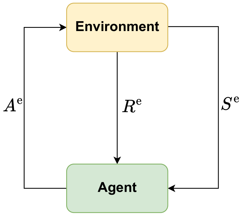
(a) MDP framework

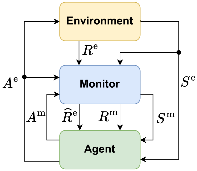
(b) Mon-MDP framework

Figure 1: In MDPs (left) the agent interacts only with the environment and observes rewards at all times. In Mon-MDPs (right), the agent also interacts with the monitor, which dictates what rewards the agent observes.

Recently, inspired by partial monitoring (Bartók et al., 2014), Parisi et al. (2024b) extended the MDP framework to also consider partially observable rewards by proposing the Monitored MDP (Mon-MDP) framework. In Mon-MDPs, the observability of the reward is dictated by a “Markovian entity” (the monitor), thus actions can have either immediate or long-term effects on the reward observability. For example, rewards may become observable only after pressing a button in the environment, or as long as the agent carries some special item, or only in areas where instrumentation is present. This opens avenues for model-based methods that try to model the process governing the reward observability, in order to plan what rewards to observe or to plan visits to states where rewards are more likely to be observed. In the next sections, we 1) define Mon-MDPs as an extension of MDPs, 2) define optimality when some rewards may never be observable, and 3) highlight how our algorithm addresses current limitations and open challenges.

(a) LEFT’s outcome cannot be observed and will always be unknown.

(b) A pessimistic agent assumes the worst (snake) for LEFT.

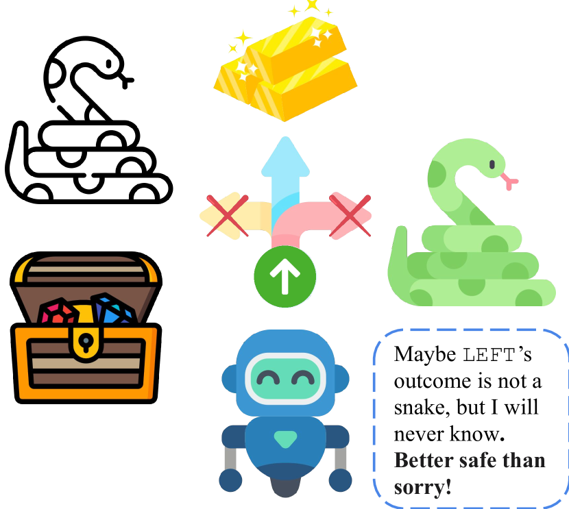
(c) The agent would be pessimistic even if LEFT’s true outcome is not the snake.

Figure 2: Example of a pessimistic agent in Mon-MDPs. (a) The agent has to choose between LEFT, UP, and RIGHT. RIGHT leads to a snake, UP to gold bars, and LEFT to either a snake or a treasure chest (more valuable than gold bars), but the agent can never observe the result of executing LEFT. (b) After sufficient attempts, the agent excludes LEFT because its outcome is unknown and the agent assumes the worst. (c) LEFT is ruled out even though it could actually yield the treasure chest. However, since this cannot be known, acting pessimistically complies with minimax-optimality in Equation 3. In the end, the agent explores new actions but it is also wary because some actions may never yield a reward. Thus, after enough exploration, it assumes the worst if the action outcome is still unknown.

2.1 Monitored Markov Decision Processes

MDPs are represented by the tuple $\left\langle\mathcal{S},\mathcal{A},r,P,\gamma\right\rangle$, where $\mathcal{S}$ is the finite state space, $\mathcal{A}$ is the finite action space, $r:\mathcal{S}\times\mathcal{A}\to[r_{\text{min}}^{\text{e}},r_{\text{max}}^{\text{e}}]$ is the mean of the reward function, $P:\mathcal{S}\times\mathcal{A}\to\Delta(\mathcal{S})$ is the Markovian transition dynamics, and $\gamma\in[0,1)$ is the discount factor describing the trade-off between immediate and future rewards. Mon-MDPs extend MDPs by introducing the monitor, another entity that the agent interacts with, and is also governed by Markovian transition dynamics. Intuitively, Mon-MDPs incorporate two MDPs — one for the environment and one for the monitor — and we differentiate quantities associated with each of them using superscripts “e” and “m”, respectively.

In Mon-MDPs, the state and the action spaces are composed of the environment and the monitor spaces, i.e., $\mathcal{S}\coloneq\mathcal{S}^{\text{e}}\times\mathcal{S}^{\text{m}}$ and $\mathcal{A}\coloneq\mathcal{A}^{\text{e}}\times\mathcal{A}^{\text{m}}$. At every timestep, the agent observes the state of both the environment and the monitor, and performs two actions, one for the environment and one for the monitor. The monitor also has Markovian dynamics, i.e., $P^{\text{m}}:\mathcal{S}^{\text{m}}\times\mathcal{A}^{\text{m}}\times\mathcal{S}^{\text{e}}\times\mathcal{A}^{\text{e}}\to\Delta(\mathcal{S}^{\text{m}})$, and the joint transition dynamics is denoted by $P\coloneq P^{\text{e}}\otimes P^{\text{m}}:\mathcal{S}\times\mathcal{A}\to\Delta(\mathcal{S})$. Note the monitor transition depends on the environment state and action, highlighting the interplay between the monitor and the environment.

Mon-MDPs have two rewards as well, $r\coloneq\left(r^{\text{e}},r^{\text{m}}\right)$, where $r^{\text{m}}:\mathcal{S}^{\text{m}}\times\mathcal{A}^{\text{m}}\to[r_{\text{min}}^{\text{m}},r_{\text{max}}^{\text{m}}]$ is also bounded. However, unlike MDPs, the environment rewards are not directly observable. Instead, the agent observes proxy rewards $\widehat{R}^{\text{e}}\sim f^{\text{m}}$, where $f^{\text{m}}:\mathbb{R}\times\mathcal{S}^{\text{m}}\times\mathcal{A}^{\text{m}}\to\mathbb{R}\cup\{\bot\}$ is the monitor function and $\bot$ denotes an “unobserved reward”, i.e., the agent does not receive any numerical reward. Using the above notation, Mon-MDPs can be compactly denoted by the tuple $M=\left\langle\mathcal{S},\mathcal{A},P,r,f^{\text{m}},\gamma\right\rangle$. Figure 1 illustrates the agent-environment-monitor interaction.

In Mon-MDPs, the agent executes joint actions $A_{t}\coloneqq(A^{\text{e}}_{t},A^{\text{m}}_{t})$ at the joint state $S_{t}\coloneqq(S^{\text{e}}_{t},S^{\text{m}}_{t})$. In turn, the environment and monitor states change and produce a joint reward $(R^{\text{e}}_{t},R^{\text{m}}_{t})$, but the agent observes $(\widehat{R}^{\text{e}},R^{\text{m}}_{t})$. The agent’s goal is to learn a policy $\pi:\mathcal{S}\to\Delta(\mathcal{A)}$ selecting joint actions to maximize the discounted return ${\sum}_{t=1}^{\infty}\gamma^{t-1}\left(R^{\text{e}}_{t}+R^{\text{m}}_{t}\right)$ even though the agent observes $\widehat{R}^{\text{e}}_{t}$ instead of $R^{\text{e}}_{t}$. This is the crucial difference between MDPs and Mon-MDPs: the immediate environment reward $R^{\text{e}}_{t}$ is always generated by the environment, i.e., desired behavior is well-defined as the reward is sufficient to fully describe the agent’s task (Bowling et al., 2023). However, the monitor may “hide it” from the agent, possibly even always yielding “unobservable reward” $\widehat{R}^{\text{e}}_{t}=\bot$ at all times for some states. For example, consider a task where the reward is given by a human supervisor (the monitor): if the supervisor must leave, the agent will not observe any reward; yet, the task has not changed, i.e., the human — if present — would still give the same rewards.

2.2 Learning Objective in Mon-MDPs

Following MDP notation, we define the V-function $V^{M}_{\pi}$ and the Q-function $Q^{M}_{\pi}$ as the expected sum of the discounted rewards, and an optimal policy $\pi^{*}$ as their maximizer:

$$V^{M}_{\pi}(s) \coloneqq\mathbb{E}_{\pi}\left[{\sum_{k=t}^{\infty}\gamma^{k-t}(R^{\text{e}}_{k}+R^{\text{m}}_{k})\mid S_{t}=s}\right],$$

$$Q^{M}_{\pi}(s,a) \coloneqq\mathbb{E}_{\pi}\left[{\sum_{k=t}^{\infty}\gamma^{k-t}(R^{\text{e}}_{k}+R^{\text{m}}_{k})\mid S_{t}=s,A_{t}=a}\right],$$

$$\pi^{*} \in\operatorname*{argmax}_{\pi\in\Pi}V_{\pi}^{M}(s)\quad\quad\forall s\in\mathcal{S},$$ (1)

where $R^{\text{e}}_{k}$ and $R^{\text{m}}_{k}$ are the immediate environment and monitor rewards at timestep $k$. We stress once more that the agent cannot observe $R^{\text{e}}$ directly and observes $\widehat{R}^{\text{e}}$, even though the environment still assigns rewards to the agent’s actions.

Parisi et al. (2024b) showed it is possible to asymptotically converge to an optimal policy if the monitor function $f^{\text{m}}$ is ergodic, i.e., if for all environment pairs $(s^{\text{e}},a^{\text{e}})$ the proxy reward will be observable ($\widehat{R}^{\text{e}}\neq\bot$) given infinite exploration. Intuitively, this means the agent will be always able to observe every environment reward (infinitely many times, given infinite exploration). However, if even one environment reward is never observable, the Mon-MDP is unsolvable and we cannot guarantee convergence to an optimal policy. Intuitively, if the agent can never know that a certain state yields the highest (or lowest) environment reward, then it can never learn to visit (or avoid) it. Nonetheless, we argue that assuming every environment reward is observable (sooner or later) is a very stringent condition, not suitable for real-world tasks — reward instrumentation may have limited coverage, human supervisors may never be available in the evening, or training before deployment may not guarantee full state coverage.

We follow Parisi et al. (2024b, Appendix B.3) in defining reasonable behavior in an unsolvable Mon-MDP. First, let $[M]_{\mathbb{I}}$ be the set of all Mon-MDPs the agent cannot distinguish based on the reward observability in $M$. If $M$ is solvable, all rewards can be observed and $[M]_{\mathbb{I}}=\{M\}$. Otherwise, from the agent’s perspective, there are possibly infinitely many Mon-MDPs in $[M]_{\mathbb{I}}$ because never-observable rewards could be any real number withing their bounded range. Second, let $M_{\downarrow}$ be the worst-case Mon-MDP, i.e., the one where all never-observable rewards are $-r_{\text{max}}^{\text{e}}$:

$$\vskip-3.0ptM_{\downarrow}\in\operatorname*{argmin}_{M^{\prime}\in[M]_{\mathbb{I}}}V_{\pi^{*}}^{M^{\prime}}(s)\quad\quad\forall s\in\mathcal{S}$$ (2)

i.e., $M_{\downarrow}$ is a Mon-MDP whose optimal value function is minimized over all Mon-MDPs indistinguishable from $M$. Then, we define the minimax-optimal policy of $M$ as the optimal policy of the worst-case Mon-MDP, i.e.,

$$\pi^{*}_{\downarrow}\coloneq\operatorname*{argmax}_{\pi}\,V_{\pi}^{M_{\downarrow}}(s).$$ (3)

If $M$ is solvable then $[M]_{\mathbb{I}}=\{M\}$, and Equation 3 is equivalent to Equation 1. So the minimax-optimal policy is simply the optimal policy. Footnote 3 shows an example of an unsolvable Mon-MDP and the minimax-optimal policy.

3 Monitored Model-Based Interval Estimation

We propose a novel model-based algorithm to exploit the structure of Mon-MDPs, show how to apply it on solvable and unsolvable Mon-MDPs, and provide sample complexity bounds. As our algorithm builds upon MBIE and MBIE-EB Strehl and Littman (2008), we first briefly review both.

3.1 MBIE and MBIE-EB

MBIE is an algorithm for learning an optimal policy in MDPs with polynomial sample complexity bounds. MBIE maintains confidence intervals on all unknown quantities (e.g., rewards and transition dynamics) and then solves the set of corresponding MDPs to produce an optimistic value function. Greedy actions with respect to this value function direct the agent toward state-action pairs that have not been sufficiently visited to be certain whether they are part of the optimal policy or not. MBIE-EB is a simpler variant that constructs one model of the MDP with exploration bonuses to be optimistic with respect to the uncertain quantities.

Let $\tilde{R}$ and $\tilde{P}$ be maximum likelihood estimates of the MDP’s unknown reward and transition dynamics based on the agent’s experience, and let $N(s,a)$ count the number of times action $a$ has been taken in state $s$. MBIE-EB constructs an optimistic MDP,

$$\bar{R}(s,a)=\tilde{R}(s,a)+\underbrace{\frac{\beta}{\sqrt{N(s,a)}}}_{\text{bonus for $R,P$}},\quad\quad\bar{P}=\tilde{P},$$ (4)

where $\beta$ is a parameter chosen to be sufficiently large. It then solves this MDP to find $\bar{Q}_{*}$, the optimal Q-function under the model, and acts greedily with respect to this value function to gather more data to update its MDP model.

3.2 Monitored MBIE-EB

Monitored MBIE-EB can be considered an extension of MBIE-EB to the Mon-MDP setting with three important innovations. First, we adapt MBIE-EB to model each of the vital unknown components of the Mon-MDP (reward and transition dynamics of both the environment and the monitor), each with their own exploration bonuses. Second, observing that the optimism for unobservable environment state-action pairs in an unsolvable Mon-MDP will never vanish — the agent will try forever to observe rewards that are actually unobservable — we further adapt the algorithm to make worst-case assumptions on all unobserved environment rewards. Unfortunately, this creates an additional problem: environment state-action pairs whose rewards are hard to observe may never be sufficiently tried because they are dissuaded by the pessimistic model. Third, Monitored MBIE-EB balances this minimax objective by interleaving a second MBIE-EB instance that ensures sufficient exploration of unobserved environment state-actions. We describe these innovations in order.

First Innovation: Extend MBIE-EB to Mon-MDPs. Let $\tilde{R}^{\text{e}},\tilde{R}^{\text{m}},\tilde{P}$ be maximum likelihood estimates of the environment reward, monitor reward, and the joint transition dynamics, respectively, all based on the agent’s experience. Let $N(s^{\text{m}},a^{\text{m}})$ count the number of times action $a^{\text{m}}$ has been taken in $s^{\text{m}}$, $N(s,a)$ count the same joint state-action pairs, and $N(s^{\text{e}},a^{\text{e}})$ count environment state-action pairs, but only if the environment reward was observed. We can then construct the following optimistic MDP using reward bonuses for the unknown estimated quantities,

$$\bar{R}_{\text{basic}}(s,a)=\, \tilde{R}^{\text{e}}(s^{\text{e}},a^{\text{e}})+\overbrace{\frac{\beta^{\text{e}}}{\sqrt{N(s^{\text{e}},a^{\text{e}})}}}^{\text{bonus for $R^{\text{e}}$}}+$$

$$\,\tilde{R}^{\text{m}}(s^{\text{m}},a^{\text{m}})+\underbrace{\frac{\beta^{\text{m}}}{\sqrt{N(s^{\text{m}},a^{\text{m}})}}}_{\text{bonus for $R^{\text{m}}$}}+\underbrace{\frac{\beta}{\sqrt{N(s,a)}}}_{\text{bonus for $P$}},$$

$$\bar{P}=\, \tilde{P},$$ (5)

where $\beta$, $\beta^{\text{e}}$, $\beta^{\text{m}}$ are hyperparameters for the confidence level of our optimistic MDP. As with MBIE-EB, this optimistic model is solved to find $\bar{Q}_{*}$ and actions are selected greedily. For solvable Mon-MDPs, we can apply MBIE-EB’s theoretical result directly to the joint MDP to get a sample complexity bound for this approach. But, this algorithm fails to make any guarantees for unsolvable Mon-MDPs, where some environment rewards are never-observable. In such situations, $N(s^{e},a^{e})$ never grows for some state-action pairs, thus optimism will direct the agent to seek out these state-actions, for which it can never reduce its uncertainty.

Second Innovation: Pessimism Instead of Optimism. We fix this excessive optimism in Equation 5 by creating a new reward model that is pessimistic, rathter than optimistic, about unobserved environment state-action rewards:

$$\bar{R}_{\text{optimize}}(s,a)= \,\begin{cases}\bar{R}_{\text{basic}}(s,a)&\text{if $N(s^{\text{e}},a^{\text{e}})>0$}\\ \bar{R}_{\text{min}}(s,a)&\text{otherwise},\end{cases}$$ (6)

where,

$$\bar{R}_{\text{min}}(s,a)= \,r^{\text{e}}_{\min}+\tilde{R}^{\text{m}}(s^{\text{m}},a^{\text{m}})\,+$$

$$\frac{\beta^{\text{m}}}{\sqrt{N(s^{\text{m}},a^{\text{m}})}}+\frac{\beta}{\sqrt{N(s,a)}}.$$ (7)

We call an episode where we take greedy actions according to $\bar{Q}_{*,\text{optimize}}$ an optimize episode, as this ideally produces a minimax-optimal policy for all Mon-MDPs. The reader may have already realized this pessimism will introduce a new problem — dissuading the agent from exploring to observe previously unobserved environment rewards. Instead, we aim to observe all rewards but not too frequently that we prevent the agent from following the minimax-optimal policy when the Mon-MDP is actually unsolvable.

Third Innovation: Explore to Observe Rewards. We fix this now excessive pessimism by introducing a separate MBIE-guided exploration aimed at discovering previously unobserved environment rewards. The following reward model does exactly that.

$$\bar{R}_{\text{observe}}(s,a) =\begin{array}[t]{l}\frac{\beta^{\text{observe}}}{\sqrt{N(s,a)}}+\\[10.0pt] \text{KL-UCB}(N(s,a))\mathds{1}\scriptstyle{\{N(s^{\text{e}},a^{\text{e}})=0\}},\end{array}$$ (10)

where $\mathds{1}\scriptstyle{\{N(s^{\text{e}},a^{\text{e}})=0\}}$ is an indicator function returning 1 if $N(s^{\text{e}},a^{\text{e}})=0$ and 0 otherwise. Therefore, the KL-UCB Garivier and Cappé (2011) term is only included for environment state-action pairs whose rewards have not been observed. We are using KL-UCB to estimate an upper-confidence bound (with confidence $\beta^{\text{KL-UCB}}$) on the probability of observing the environment reward from joint state-action $(s,a)$ given that we tried $N(s,a)$ times already and have not succeeded. As we are constructing a bound on a Bernoulli random variable (whether the reward is observed or not), KL-UCB is ideally suited and provides tight bounds. The result is an optimistic model for an MDP that rewards the agent for observing previously unobserved environment rewards (if they can be observed). An episode where we take greedy actions with respect to $\bar{Q}_{*,\text{observe}}$ we call an observe episode. If we have enough observe episodes, we can guarantee that all observable environment rewards are observed with high probability. If we have enough optimize episodes we can learn and follow the minimax-optimal policy. We balance between the two by switching the model we optimize according to the following condition

$$\bar{R}(s,a) =\left\{\begin{array}[]{ll}\bar{R}_{\text{observe}}(s,a)&\text{if $\kappa\leq\kappa^{*}(k)$}\\ \bar{R}_{\text{optimize}}(s,a)&\text{otherwise},\end{array}\right.$$ (13)

where $\kappa^{*}$ is a sublinear function returning how many episodes of the $k$ total episodes should have been used to observe and $\kappa$ is the number of episodes that have been used to observe. The choice of $\kappa^{*}$ is a hyperparameter. Monitored MBIE-EB then constructs the $\{\bar{R}(s,a),\bar{P}(s,a)\}$ MDP model and selects greedy actions with the respect to its optimal Q-function $\bar{Q}_{*}$. The choice to hold the policy fixed throughout the course of an episode is a matter of simplicity, giving easier analysis that observe episodes will observe environment rewards, as well as computational convenience.

3.3 Theoretical Guarantees

Monitored MBIE-EB has a polynomial sample complexity even in unsolvable Mon-MDPs. There exists parameters where the algorithm guarantees with high probability ($1-\delta$) of being arbitrarily close to minimax-optimal ($\varepsilon$) for all but a finite number of time steps, which is a polynomial of $\nicefrac{{1}}{{\varepsilon}}$, $\nicefrac{{1}}{{\delta}}$, and other quantities characterizing the Mon-MDP. This gives the first sample complexity bound for Mon-MDPs.

Theorem 3.1.

For any $\varepsilon,\delta>0$, and Mon-MDP $M$ where $\rho$ is the minimum non-zero probability of observing the environment reward in $M$ and $H$ is the maximum episode length, there exists constants $m_{1}$, $m_{2}$, and $m_{3}$ where

$$m_{1} =\tilde{\mathcal{O}}\left(\frac{|\mathcal{S}|}{\varepsilon^{2}(1-\gamma)^{4}}\right)$$

$$m_{2} =\tilde{\mathcal{O}}\left(\frac{r_{\text{max}}^{\text{e}}(r_{\text{max}}^{\text{e}}+r_{\text{max}}^{\text{m}})^{2}}{\rho\varepsilon^{2}(1-\gamma)^{4}}\right)$$

$$m_{3} =\tilde{\mathcal{O}}\left(\frac{\left\lvert\mathcal{S}\right\rvert^{2}\left\lvert\mathcal{A}\right\rvert}{\varepsilon^{3}(1-\gamma)^{5}}\right)$$

such that Monitored MBIE-EB with parameters,

$$\beta =\gamma(r_{\text{max}}^{\text{e}}+r_{\text{max}}^{\text{m}})\sqrt{2\ln{(12\left\lvert\mathcal{S}\right\rvert\left\lvert\mathcal{A}\right\rvert m_{2}/\delta)}}\big{/}(1-\gamma)$$

$$\beta^{\text{m}} =r_{\text{max}}^{\text{m}}\sqrt{2\ln{(12\left\lvert\mathcal{S}\right\rvert\left\lvert\mathcal{A}\right\rvert m_{2}/\delta)}}$$

$$\beta^{\text{e}} =r_{\text{max}}^{\text{e}}\sqrt{2\ln{(12\left\lvert\mathcal{S}\right\rvert\left\lvert\mathcal{A}\right\rvert m_{2}/\delta)}}$$

$$\beta^{\text{observe}} =\left({1}\big{/}{(1-\gamma)}\sqrt{\ln{\left(\nicefrac{{8\left\lvert\mathcal{S}\right\rvert\left\lvert\mathcal{A}\right\rvert m_{1}}}{{\delta}}\right)}\big{/}{2}}\right)$$

$$\beta^{\text{KL-UCB}} =\ln(\nicefrac{{8\left\lvert\mathcal{S}\right\rvert\left\lvert\mathcal{A}\right\rvert m_{1}}}{{\delta}})$$

$$\kappa^{*}(k) =m_{3}\quad\quad\text{(constant function)}$$

provides the following bounds for $M$. Let $\pi_{t}$ denote Monitored MBIE-EB’s policy and $s_{t}$ denote the state at time $t$. With probability at least $1-\delta$, $V^{M_{\downarrow}}_{\pi_{t}}(s_{t})\geq V^{M_{\downarrow}}_{\pi^{*}}-\varepsilon$ for all but $\tilde{\mathcal{O}}\left(\dfrac{r_{\text{max}}^{\text{e}}(r_{\text{max}}^{\text{e}}+r_{\text{max}}^{\text{m}})\left\lvert\mathcal{S}\right\rvert\left\lvert\mathcal{A}\right\rvert H}{\varepsilon^{3}(1-\gamma)^{5}\rho}\right)$ timesteps.

The reader may refer to Appendix F for the proof.

An interesting addition to the bound over MBIE bounds for traditional MDPs is the dependence on $\rho$, which bounds how difficult it is to observe the observable environment rewards. If a Mon-MDP does reveal all rewards (it is solvable) but only does so with infinitesimal probability, an algorithm must be suboptimal for many more time steps.

3.4 Practical Implementation

The theoretically justified parameters for Monitored MBIE-EB present a couple of challenges in practice. First off, we rarely have a particular $\epsilon$ and $\delta$ in mind, preferring algorithms that produce ever-improving approximations with ever-improving probability. Second, the bound, while polynomial in the relevant values, does not suggest practical parameters. The most problematic in this regard is the constant $\kappa^{*}$, which places all observe episodes at the start of training. Third, solving an MDP model exactly and from scratch each episode to compute $\bar{Q}_{*}$ is computationally wasteful.

In practice, we slowly increase the confidence levels used in the exploration bonuses over time. We follow the pattern of Lattimore and Szepesvári (2020), with the confidence growing slightly faster than logarithmically. The scale parameters $\beta$, $\beta^{\text{m}}$, $\beta^{\text{e}}$, $\beta^{\text{observe}}$, $\beta^{\text{KL-UCB}}$ were then tuned manually for each environment. For $\kappa^{*}$ we also grow it slowly over time allowing the agent to interleave observe and optimize episodes: $\kappa^{*}(k)=\log k$, where the log base was also tuned manually for each environment. Finally, rather than exactly solving the models every episode, we maintain two value functions: $\bar{Q}_{\text{observe}}$ and $\bar{Q}_{\text{optimize}}$, both initialized optimistically. we do 50 steps of synchronous value iteration before every episode to improve $\bar{Q}_{\text{optimize}}$, and before observe episodes to improve $\bar{Q}_{\text{observe}}$.

(a) River Swim

(b) Bottleneck

Figure 3: Environments

Discounted Test Return

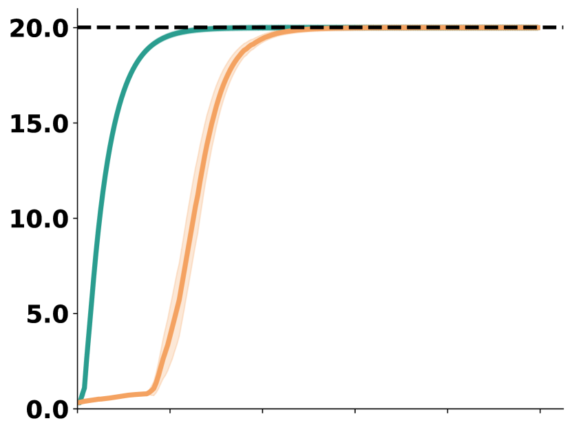
Training Steps ($\times 10^{3}$)

(c) River Swim

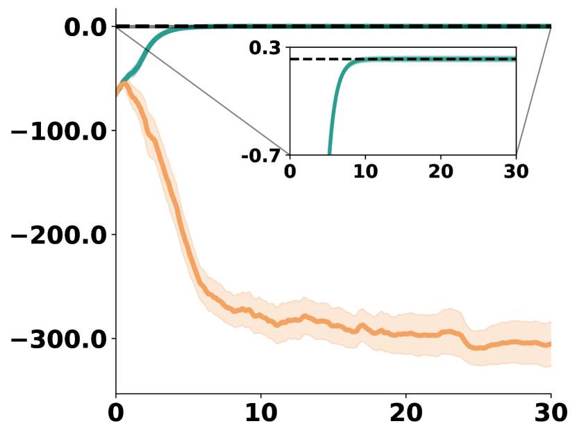
Training Steps ($\times 10^{3}$)

(d) Bottleneck (100%)

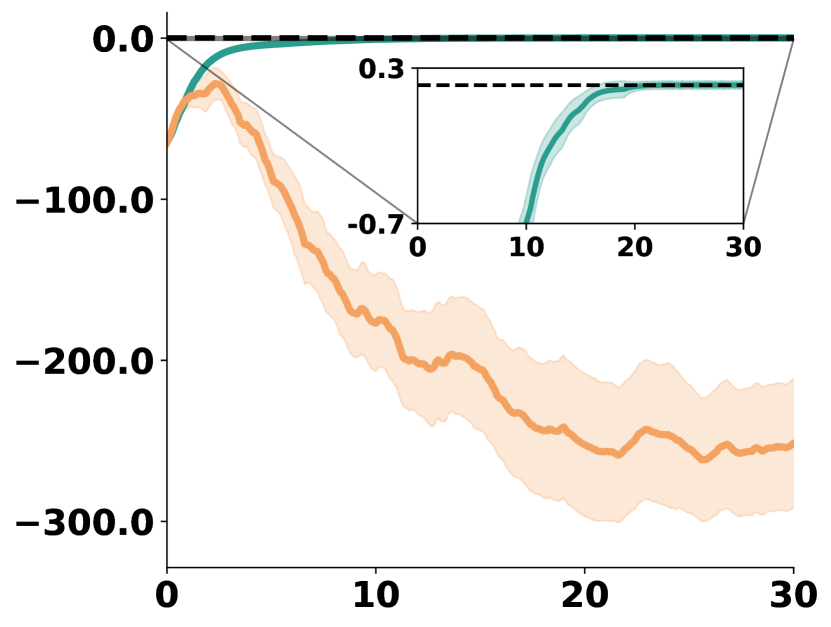
Training Steps ($\times 10^{3}$)

(e) Bottleneck (5%)

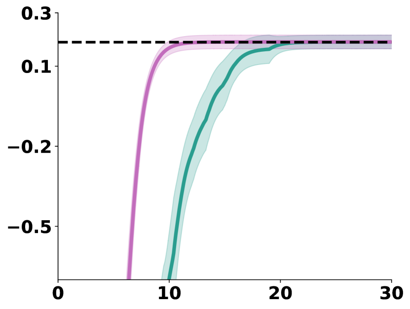
Training Steps ($\times 10^{3}$)

(f) Bottleneck (5%)

Figure 4: Discounted return at test time, averaged over 30 seeds (shaded areas denote 95% confidence intervals). Monitored MBIE-EB (in green) outperforms Directed-E² (in orange) and always converges to the minimax-optimal policy (the dashed black line). (c) and (d) both show results in the Bottleneck with the 5% Button Monitor, but with different axis ranges to highlight the improvement if Monitored MBIE-EB already knows details of the monitor (in purple).

4 Empirical Evaluation

This paper began by detailing limitations in prior work not taking advantage of the Mon-MDP structure, the possibility of a known monitor, nor dealing with unsolvable Mon-MDPs with unobservable rewards. This section breaks down this claim into four research questions (RQ) to investigate if Monitored MBIE-EB can:

1. Explore efficiently in hard-exploration tasks?

2. Act pessimistically when rewards are unobservable?

3. Identify and learn about difficult to observe rewards?

4. Take advantage of a known model of the monitor?

To directly address these questions, we first show results on two tasks with two monitors. Then, we show results on 24 benchmarks to strengthen our claims.

4.1 Environment and Monitor Description

River Swim (Figure 3(a)) is a well-known difficult exploration task with two actions. Moving LEFT always succeeds, but moving RIGHT may not — the river current may cause the agent to stay at the same location or even be pushed to the left. There is a goal state on the far right, where $R^{\text{e}}=1$. However, the leftmost tile yields $R^{\text{e}}=0.1$ and it is much easier to reach. Other states have zero rewards. Agents often struggle to find the optimal policy (always move RIGHT), and instead converge to always move LEFT. In our experiments, we pair River Swim with the Full Monitor where environment rewards are always freely observable, allowing us to focus on an algorithm’s exploration ability.

Bottleneck (Figure 3(b)) has five deterministic actions: LEFT, UP, RIGHT, DOWN, STAY, which move the agent around the grid. Episodes end when the agent executes STAY in either the gold bars state ($R^{\text{e}}=0.1$) or in the treasure chest state ($R^{\text{e}}=1$). Reaching the snake state yields $R^{\text{e}}=-10$, and other states yield $R^{\text{e}}=0$. However, states denoted by $\bot$ have never-observable rewards of -10, i.e., $R^{\text{e}}=-10$ but $\widehat{R}^{\text{e}}=\bot$ at all times. In our experiments, we pair Bottleneck with the Button Monitor, where the monitor state can be ON or OFF (initialized at random) and can be switched if the agent executes DOWN in the button state. When the monitor is ON, the agent receives $R^{\text{m}}=-0.2$ at every timestep, but also observes the current environment reward (unless the agent is in a $\bot$ state). The optimal policy follows the shortest path to the treasure chest, while avoiding the snake and $\bot$ states, and turning the monitor OFF if it was ON at the beginning of the episode. To evaluate how Monitored MBIE-EB performs when observability is stochastic, we consider two versions of the Button Monitor: one where the monitor works as intended and rewards are observable with 100% probability if ON, and a second where the rewards are observable only with 5% probability if ON.

Visitation Count

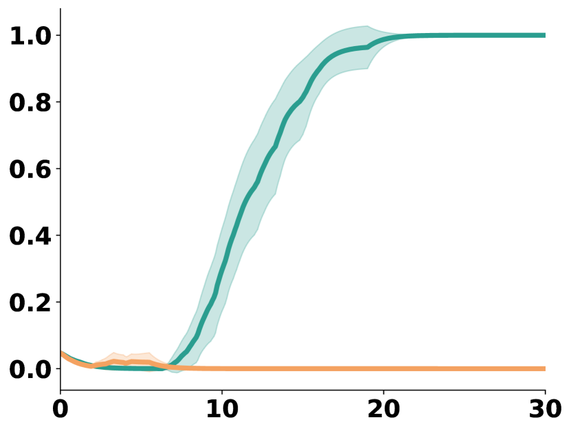
Training Steps ($\times 10^{3}$)

(a) Visits to the goal

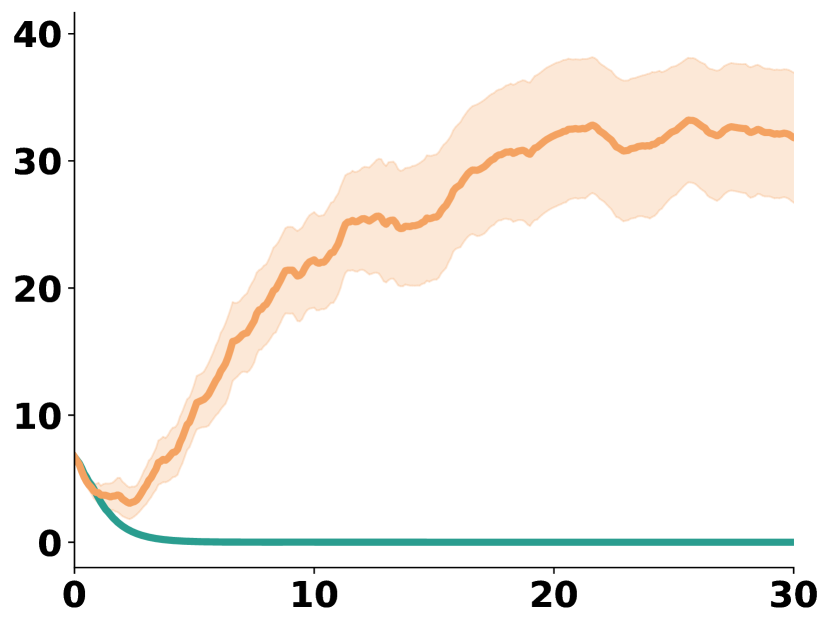
Training Steps ($\times 10^{3}$)

(b) Visits to $\bot$

Figure 5: Visits to important states at test time in the Bottleneck with 5% Button Monitor. Results are averaged over 30 trials, and shaded areas denote 95% confidence interval. Directed-E² fails to focus on the goal and instead keeps visiting $\bot$ states, whereas Monitored MBIE-EB reduces its visitation frequency instead, ultimately visiting only the goal.

4.2 Results

We compare Monitored MBIE-EB against Directed Exploration-Exploitation (Directed-E²) (Parisi et al., 2024a), which is, to the best of our knowledge, currently the most performant algorithm in Mon-MDPs. In all benchmarks, the discount factor is $\gamma=0.99$. The full set of hyperparameters are in Appendix C are full evaluation details (e.g., episodes lengths, evaluation frequencies) are in Appendix B. Results shown in Figures 4 and 5 are at test time, i.e., when the agent follows the current greedy policy without exploring.

To answer RQ1, consider the results in Figure 3(c). In this case, the performance of Monitored MBIE-EB significantly outperforms that of Directed-E². This task is difficult for any $\epsilon$-greedy exploration strategy (such as the one of Directed-E²) and highlights the first innovation: taking a model-based approach in Mon-MDPs (i.e., extending MBIE-EB) allows Monitored MBIE-EB to have more efficient exploration.

To answer RQ2, consider Figure 3(d). In this case, states marked with $\bot$ are never observable by the agent, regardless of the monitor state. Because the minimum reward in this task is $r_{\text{min}}=-10$, the minimax-optimal policy is to avoid states marked by $\bot$ while reaching the goal state ($R^{\text{e}}=1$). Monitored MBIE-EB is able to find this optimal policy, whereas Directed-E² does not because it does not learn to avoid unobservable rewards. This result highlights the impact of the second innovation: unsolvable Mon-MDPS require pessimism when the reward cannot be observed.

To answer RQ3, consider Figure 3(e), where the Button Monitor provides a reward only 5% of the time when ON (and 0% of the time when OFF). Despite how difficult it is to observe rewards, Monitored MBIE-EB is able to learn the minimax-optimal policy. This shows that Monitored MBIE-EB is still appropriately pessimistic, successfully avoiding $\bot$ states and the snake, and reaching the better goal state. Since rewards are only visible one out of twenty times (when the monitor is ON), learning is much slower than in Figure 3(d), matching the appearance of $\rho$ in Theorem 3.1’s bound. This result also shows the impact of the third innovation: it is important to explore just enough to guarantee that the agent will learn about observable rewards, but no more. This result highlights the impact of the third innovation.

To answer RQ4, now consider the performance of Known Monitor in Figure 3(f), showing the performance of Monitored MBIE-EB when provided the model of the Button Monitor 5%. Results show that its convergence speed increases significantly, as Monitored MBIE-EB takes (on average) 30% fewer steps to find the optimal policy. This feature of Monitored MBIE-EB is particularly important in settings where the agent has already learned about the monitor previously or the practitioner can provide the agent with an accurate model of the monitor. The agent, then, needs only to learn about the environment, and does not need to explore the monitor component of the Mon-MDP.

Discounted Test Return
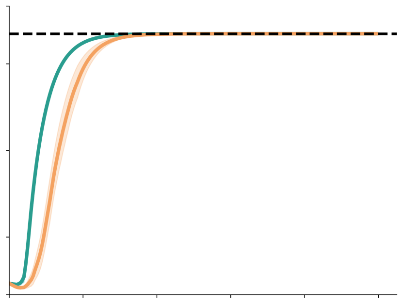
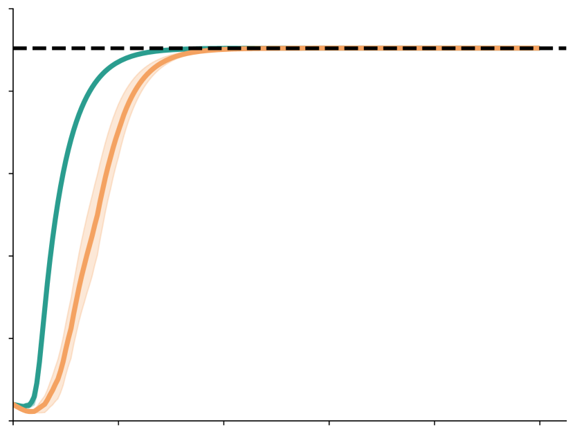
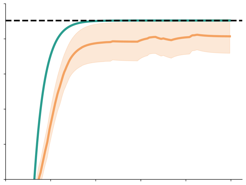
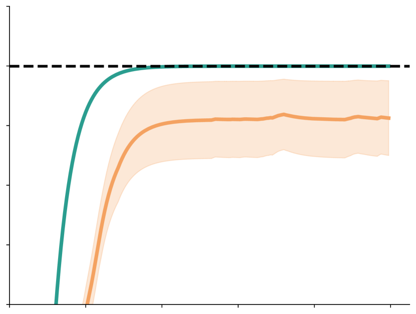
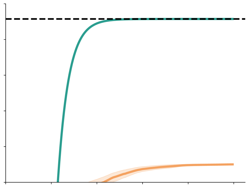
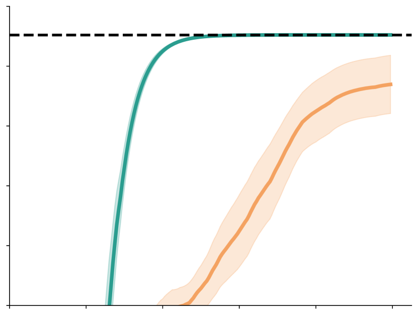
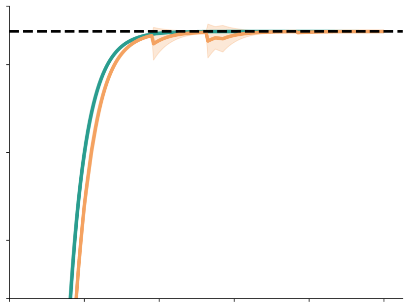
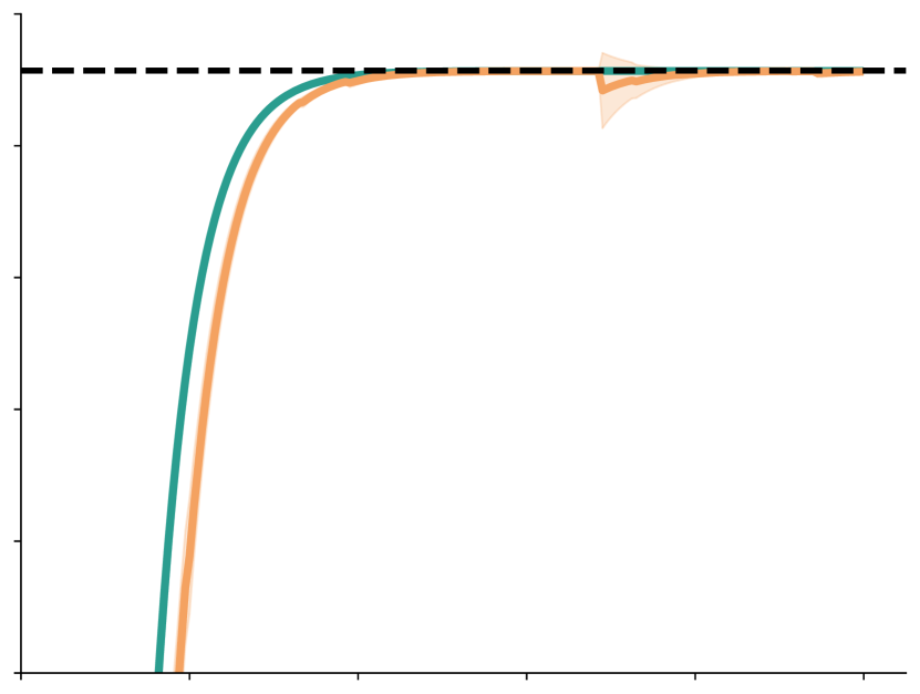
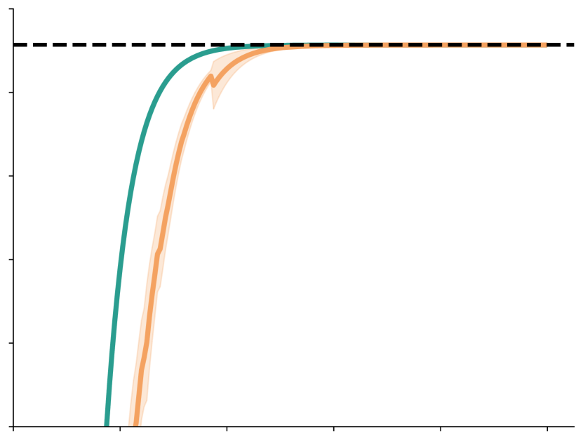
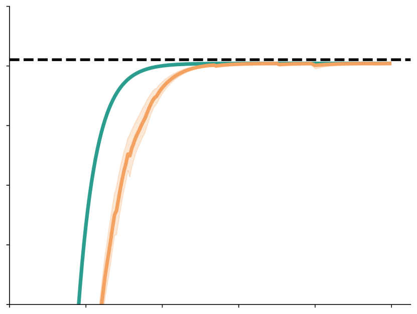
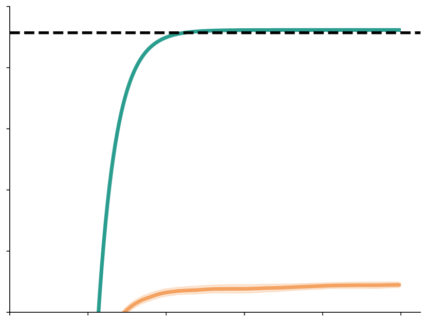
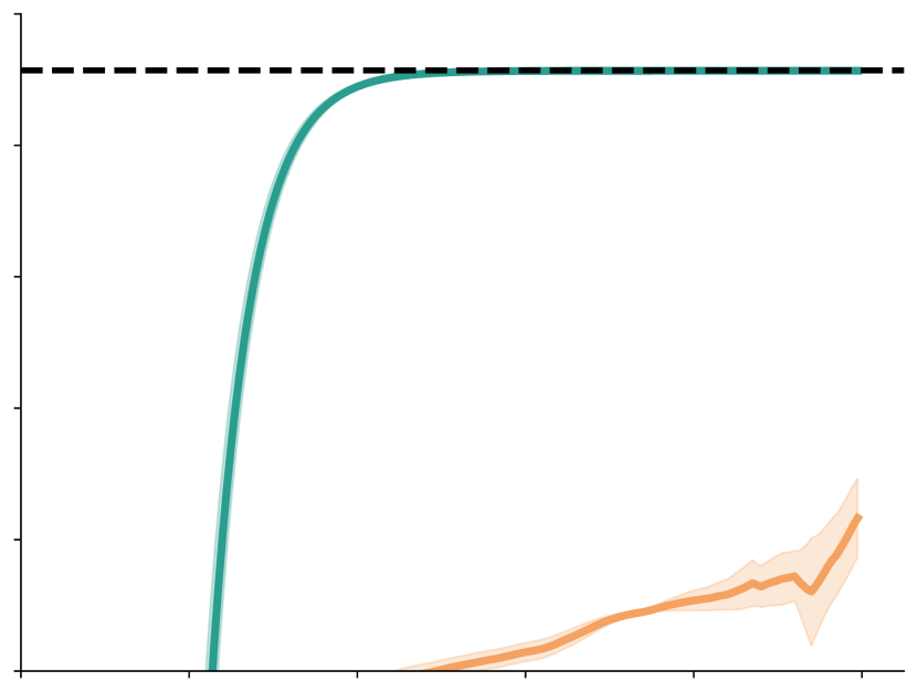
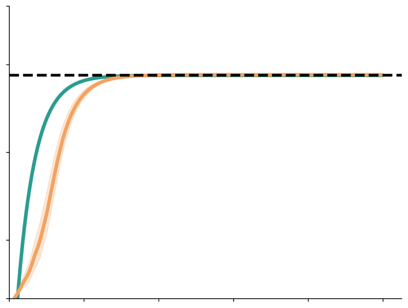
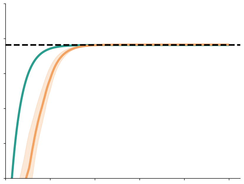
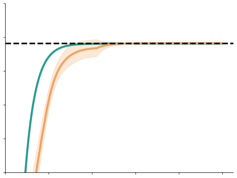
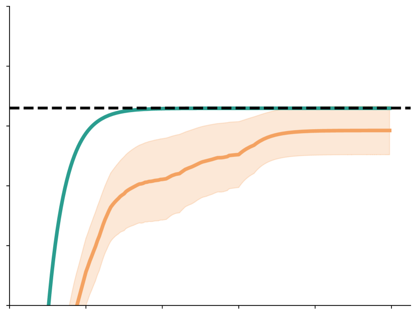
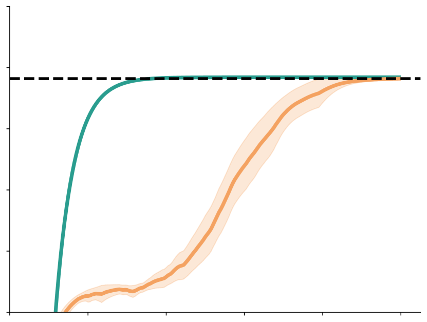
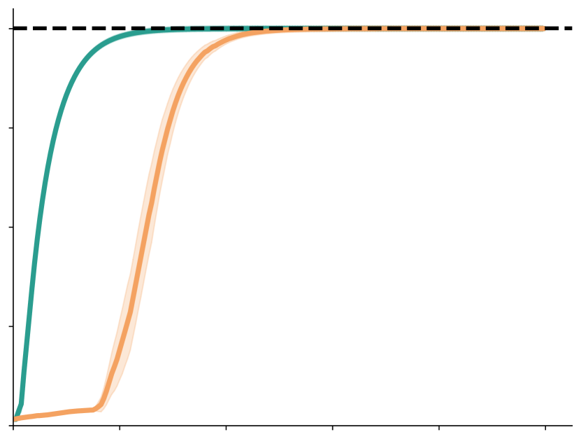
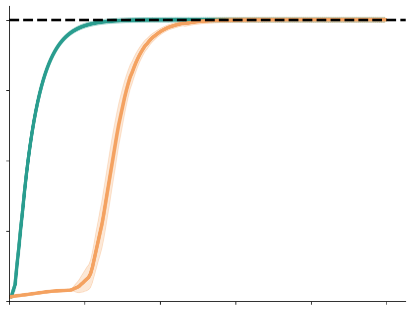
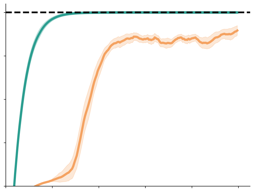
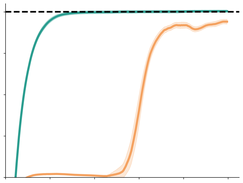
 Training Steps

Figure 6: Performance on 24 benchmark environments from Parisi et al. (2024a). Monitored MBIE-EB clearly outperforms Directed-E² in 22 of them and performs on par in the remainder two. Full-size graphs with details of all 24 benchmarks are in Section B.3.

To better understand the above results, Figure 5 shows how many times the agent visits the goal state and $\bot$ states per testing episode. Both algorithms initially visit the goal state (Figure 5(a)) during random exploration (i.e., when executing the policy after 0 timesteps of training). Monitored MBIE-EB appropriately explores for some training episodes (recall that rewards are only observed in ON and even then only 5% of the time), and then learns to always go to the goal. Both also initially visit $\bot$ states (Figure 5(b)). However, while Monitored MBIE-EB learns to be appropriately pessimistic over time and avoids them, Directed-E² never updates its (random) initial estimate of the value of $\bot$ states and incorrectly believes they should continue to be visited. This also explains why Directed-E² performs even worse in Figure 3(e).

Finally, Figure 6 presents results comparing Monitored MBIE-EB across all of the domains and monitor benchmarks from Parisi et al. (2024a). In these 24 benchmarks, Monitored MBIE-EB significantly outperforms Directed-E² in all but 2 of them, where they perform similarly.

5 Discussion

There are a number of limitations to our approach that suggest directions for future improvements. First, Mon-MDPs contain an exploration-exploitation dilemma, but with an added twist — the agent needs to treat never observed rewards pessimistically in order to achieve a minimax-optimal solution; however, it should continue exploring those states to get more confident about their unobservability. Much like early algorithms for the exploration-exploitation dilemma in MDPs (Kearns and Singh, 2002), our approach separately optimizes a model for exploring and one for seeking a minimax-optimal solution. A more elegant approach would be to simultaneously optimize for both. Second, our approach uses explicit counts to drive its exploration, which limits it to enumerable Mon-MDPs. Adapting psuedocount-based methods (Bellemare et al., 2016; Martin et al., 2017; Tang et al., 2017; Machado et al., 2020) can help making Monitored MBIE-EB more applicable to large or continuous state spaces. Finally, the decision of when to stop trying to observe rewards and instead optimize is essentially an optimal stopping time problem (Lattimore and Szepesvári, 2020), and there may be considerable innovations that could improve the bounds along with empirical performance.

6 Conclusion

We introduced a new algorithm, Monitored MBIE-EB, for Mon-MDPs that addresses many of the shortcomings of previous algorithms. It gives the first finite-time sample complexity bounds for Mon-MDPs, while being applicable to both solvable and unsolvable Mon-MDPs, for which it is also the first. Furthermore, it both exploits the structure of the Mon-MDP and can take advantage of knowledge of the monitor process, if available. These features are not just theoretical, as we see these innovations resulting in empirical improvements in Mon-MDP benchmarks, comprehensively outperforming the previous best learning algorithms.

Impact Statement

This paper presents work whose goal is to advance the fundamental understanding of reinforcement learning. Our work is mostly theoretical and experiments are conducted on simple environments that do not involve human participants or concerning datasets, and it is not tied to specific real-world applications. We believe that our contribution has little to no potential for harmful impact.

In this Appendix we provide the full proof of the sample complexity bound of Monitored MBIE-EB, additional details about the algorithm, the full set of experiments (including description of more environment and monitors, full details of the hyperparameters, and an outline of Directed-E²).

Appendix A Table of Notation

Symbol	Explanation
$\Delta(\mathcal{X})$	$\Delta(\mathcal{X})$ denotes the set of distributions over the finite set $\mathcal{X}$
$M$	An instance of a Mon-MDP
$\mathcal{S}$	State space (environment-only in MDPs, joint environment-monitor in Mon-MDPs)
$\mathcal{A}$	Action space (environment-only in MDPs, joint environment-monitor in Mon-MDPs)
$r(s,a)$	Expected reward from taking action $a$ from state $s$
$P$	Transition probabilities in MDPs / Joint transition probabilities in Mon-MDPs
$\tilde{P}$	maximum likelihood estimate of $P$
$\gamma$	Discount factor
$r_{\text{max}}^{\text{e}}$	Maximum expected environment reward; $-r_{\text{max}}^{\text{e}}$ is the minimum
$\mathcal{S}^{\text{e}}$	Environment state space
$\mathcal{A}^{\text{e}}$	Environment action space
$R^{\text{e}}$	Immediate environment reward
$\widehat{R}^{\text{e}}$	Immediate environment proxy reward
$\tilde{R}^{\text{e}}$	Maximum likelihood estimate of $r^{\text{e}}$
$P^{\text{e}}$	Environment transition probabilities
$\mathcal{S}^{\text{m}}$	Monitor state space
$P^{\text{m}}$	Monitor transition probabilities
$f^{\text{m}}$	Monitor function
$r_{\text{max}}^{\text{m}}$	Maximum expected monitor reward; $-r_{\text{max}}^{\text{m}}$ is the minimum
$N(s,a)$	Number of times $a$ has been taken from $s$
$N(s^{\text{m}},a^{\text{m}})$	Number of times $a^{\text{m}}$ has been taken from $s^{\text{m}}$
$N(s^{\text{e}},a^{\text{e}})$	Number of times $s^{\text{e}}$ has been taken from $s^{\text{e}}$ and the reward observed
$\kappa$	Number of explore episodes
$\kappa^{*}(k)$	Desired number of explore episodes through episode $k$
$\rho$	The minimum non-zero probability of observing the environment reward

Appendix B Empirical Evaluation

Our baseline is Directed-E² as the precursor of our work that Parisi et al. [2024a] showed its superior performance on Mon-MDPs against many well-established algorithms. Directed-E² uses two action-values, one as the ordinary action-values that uses a reward model in place of the environment reward to update action-values (this sets the agent free from the partial observability of the environment reward once the reward model is learned). Second action value function denoted by $S$ is dubbed as visitation-values that tries to maximized the successor representations. Directed-E² uses visitation-values to visit every joint state-action pairs but in the limit of infinite exploration it becomes greedy with respect to the main action-values for maximizing the expected sum of discounted rewards.

Evaluations are based on the discounted test return and the results are averaged across 30 independent random seeds with their corresponding $95\%$ confidence intervals. To measure the discounted test return, after every 100 steps of the interaction, the learning is paused and the agent is tested for 100 episodes and the mean over the obtained return is used as a data point, then the learning carries on.

Empty

Hazard

Bottleneck

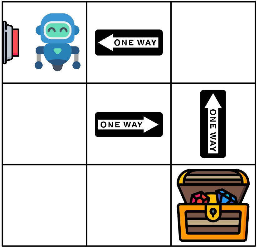
Loop

River Swim

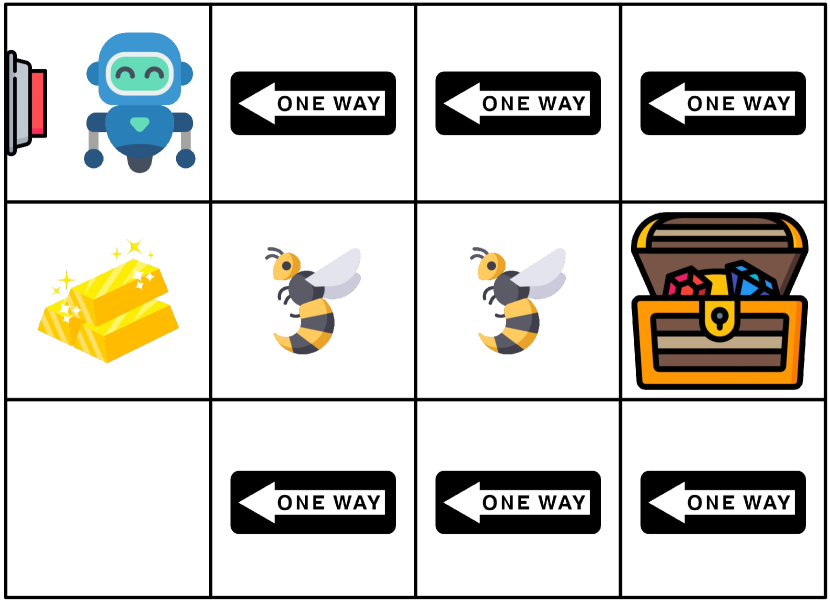
One-Way

Two-Room-2x11

Corridor

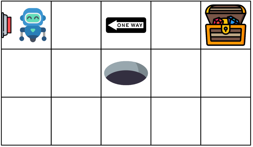
Two-Room-3x5

Figure 7: Full set of environments

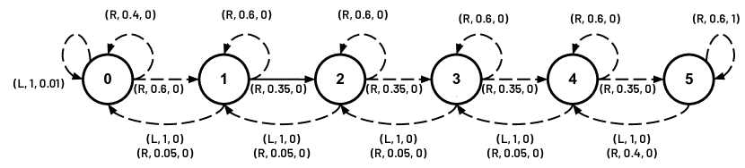
Figure 8: Dynamics of River Swim. Each tuple represents (action, transition probability, reward).

B.1 Full Environments’ Details

Environments that comprise the experiments are: Empty, Hazard, Bottleneck, Loop, River Swim, One-Way, Corridor, Two-Room-3x5 and Two-Room-2x11 shown in Figure 7. In all of them (except River Swim) the agent, represented by the robot, has 5 actions including 4 cardinal movement {LEFT, DOWN, RIGHT, UP} and an extra STAY action. its goal is get to the treasure chest as fast as possible it should STAY there to get a reward of +1 and this terminates the episode. it should not STAY at gold bars as they are distractors because it would get a reward of 0.1 and the episode gets terminated too. Snakes should be avoided as any action leading to their states results in rewards of -10. Cells with a one-way sign transition the agent only to their unique direction and if the agent stumbles on a hole, it would spend the whole episode in it, unless with probability 10% its action is effective and it gets transitioned. When a button monitor is configured on top of the environment, the location of the button is metaphorically is indicated by a push button placed on a cell’s border. It shows the button is pushed if agent bump herself into that cell’s wall. The episode’s time limit in River Swim, corridor and Two-Room-2x11 is 200 steps, and other environment it is 50 steps. In River Swim the agent has two actions L $\equiv$ LEFT and R $\equiv$ RIGHT. There is no termination except the episode’s time limit. In this environment gold bars have a reward of 0.01. And It is the only environment in our experiment suite that has stochastic transitions as in Figure 8.

B.2 Full Monitors’ Details

Monitors that comprise the experiments are: Full-Monitor (MDP), Semi-Random, Full-Random, Ask, Button, N-Supporters, N-Experts and Level-Up. For any of the monitors, except Full-Monitor, if a cell in the environment is marked with $\bot$, then under no circumstances and at no time step, the monitor would reveal the environment reward to agent for the action that led agent to that cell. For the rest of the environment state-action pairs the behavior of monitors, by letting $X_{t}\sim\mathcal{U}[0,1]$, where $\mathcal{U}$ is the uniform distribution and $\rho\in[0,1]$, is as follows :

• Full-Monitor. This corresponds to MDP setting. Monitor shows the environment reward for all environment state-action pairs. State space and action state space of the monitor are singletons and the monitor reward is zero:

  $$\mathcal{S}^{\text{m}}\coloneq\{\texttt{ON}\}, \mathcal{A}^{\text{m}}\coloneq\{\texttt{NO-OP}\}, S^{\text{m}}_{t+1}\coloneq\texttt{ON}$$

  $$\widehat{R}^{\text{e}}_{t}\coloneq R^{\text{e}}_{t},\forall t\geq 0, R^{\text{m}}_{t}\coloneq 0$$

• Semi-Random. It is similar to Full-Monitor except that non-zero environment rewards are stashed with 50% chance:

  $$\mathcal{S}^{\text{m}}\coloneq\{\texttt{ON}\}, \mathcal{A}^{\text{m}}\coloneq\{\texttt{NO-OP}\}, S^{\text{m}}_{t+1}\coloneq\texttt{ON}$$

  $$\widehat{R}^{\text{e}}_{t}\coloneq\begin{cases}R^{\text{e}}_{t}&\textbf{if }R^{\text{e}}_{t}=0\\ R^{\text{e}}_{t}&\textbf{if }X_{t}\leq 0.5\\ \bot&\text{Otherwise}\end{cases}, R^{\text{m}}_{t}\coloneq 0$$

• Full-Random. It is similar to Semi-Random except any environment reward is stashed with a predefined probability $\rho$:

  $$\mathcal{S}^{\text{m}}\coloneq\{\texttt{ON}\}, \mathcal{A}^{\text{m}}\coloneq\{\texttt{NO-OP}\}, S^{\text{m}}_{t+1}\coloneq\texttt{ON}$$

  $$\widehat{R}^{\text{e}}_{t}\coloneq\begin{cases}R^{\text{e}}_{t}&\textbf{if }X_{t}\leq\rho\\ \bot&\text{Otherwise}\end{cases} R^{\text{m}}_{t}\coloneq 0$$

• Ask. The state space is a singleton but the action space has two actions: {ASK, NO-OP}. Agent gets to see the environment reward with probability $\rho$ if it ASKs. Upon asking agent pays -0.2 as the monitor reward:

  $$\mathcal{S}^{\text{m}}\coloneq\{\texttt{ON}\}, \mathcal{A}^{\text{m}}\coloneq\{\texttt{ASK, NO-OP}\}, S^{\text{m}}_{t+1}\coloneqq\texttt{ON}$$

  $$\widehat{R}^{\text{e}}_{t}\coloneq\begin{cases}R^{\text{e}}_{t}&\textbf{if }X_{t}\leq\rho\textbf{ and }A^{\text{m}}_{t}=\texttt{ASK}\\ \bot&\text{Otherwise}\end{cases}, R^{\text{m}}_{t}\coloneq\begin{cases}-0.2&\textbf{if }A^{\text{m}}_{t}=\texttt{ASK}\\ 0&\text{Otherwise}\end{cases},$$

• Button. The state space is binary $\{\texttt{ON, OFF}\}$. The action space is a singleton. Agent gets to see the environment reward with probability $\rho$ if it manages to have the monitor be ON. The state is flipped if agent bumps herself to the wall that the button is placed on. As long as the button is ON agent pays -0.2:

  $$\mathcal{S}^{\text{m}}\coloneq\{\texttt{OFF, ON}\},$$

  $$\mathcal{A}^{\text{m}}\coloneq\{\texttt{NO-OP}\},$$

  $$\widehat{R}^{\text{e}}_{t}\coloneq\begin{cases}R^{\text{e}}_{t}&\textbf{if }X_{t}\leq\rho\textbf{ and }S^{\text{m}}_{t}=\texttt{ON}\\ \bot&\text{Otherwise}\end{cases},$$

  $$S^{\text{m}}_{t+1}\coloneq\begin{cases}\texttt{ON}&\textbf{if }S^{\text{m}}_{t}=\texttt{OFF}\textbf{ and }S^{\text{e}}_{t}=\texttt{"BUTTON-CELL"}\textbf{ and }A^{\text{e}}_{t}=\texttt{"BUMP-INTO-BUTTON"}\\ \texttt{OFF}&\textbf{if }S^{\text{m}}_{t}=\texttt{ON}\textbf{ and }S^{\text{e}}_{t}=\texttt{"BUTTON-CELL"}\textbf{ and }A^{\text{e}}_{t}=\texttt{"BUMP-INTO-BUTTON"}\\ S^{\text{m}}_{t}&\text{Otherwise}\end{cases}$$

  $$S^{\text{m}}_{1}\coloneqq\text{Random uniform from }\mathcal{S}^{\text{m}}$$

  $$R^{\text{m}}_{t}\coloneq\begin{cases}-0.2&\textbf{if }S^{\text{m}}_{t}=\texttt{ON}\\ 0&\text{Otherwise}\end{cases},$$

• N-Supporters. The state space is consisted of $N$ states that each represents the presence of a supporter. The action space is also consisted of $N$ actions. At each time step one of the supporters is randomly present and if agent could choose the action that matches the index of the supporter, then it gets to see the environment reward with probability $\rho$. Upon observing the environment reward agent pays a penalty of $-0.2$ as the monitor reward. However if it chooses a wrong supporter, then it will be rewarded $0.001$ as the monitor reward:

  $$\mathcal{S}^{\text{m}}\coloneq\{0,\cdots,N-1\}, \mathcal{A}^{\text{m}}\coloneq\{0,\cdots,N-1\}$$

  $$\widehat{R}^{\text{e}}_{t}\coloneq\begin{cases}R^{\text{e}}_{t}&\textbf{if }X_{t}\leq\rho\textbf{ and }S^{\text{m}}_{t}=A^{\text{m}}_{t}\\ \bot&\text{Otherwise}\end{cases}, R^{\text{m}}_{t}\coloneq\begin{cases}-0.2&S^{\text{m}}_{t}=A^{\text{m}}_{t}\\ 0.001&\text{Otherwise}\end{cases}$$

  $$S^{\text{m}}_{t+1}\coloneq\text{Random uniform from }\mathcal{S}^{\text{m}}$$

  Parisi et al. [2024a] introduced this monitor as being difficult due to its bigger spaces; however, the encouraging nature of the monitor regarding the agent’s mistakes makes the monitor easy for reward-respecting algorithms e.g. Monitored MBIE-EB.

• N-Experts. Similar to N-Supporter the state space has $N$ states, each corresponding the presence of $N$ experts. However getting experts’ advice is costly, hence the action space has $N+1$ action where the last action corresponds to not pinging any experts. At each time step one of the experts is randomly present and if the agent selects the action that matches the present expert’s id, it gets to see the environment reward with probability $\rho$. Upon observing the environment reward agent pays a penalty of $-0.2$ as the monitor reward. However if it chooses a wrong expert it will be penalized by $-0.001$ as the monitor reward. Since the last action does not inquire any of the experts its monitor reward is $0$:

  $$\mathcal{S}^{\text{m}}\coloneq\{0,\cdots,N-1\}, \mathcal{A}^{\text{m}}\coloneq\{0,\cdots,N\}$$

  $$\widehat{R}^{\text{e}}_{t}\coloneq\begin{cases}R^{\text{e}}_{t}&\textbf{if }X_{t}\leq\rho\textbf{ and }S^{\text{m}}_{t}=A^{\text{m}}_{t}\\ \bot&\text{Otherwise}\end{cases}, R^{\text{m}}_{t}\coloneq\begin{cases}-0.2&\textbf{if }S^{\text{m}}_{t}=A^{\text{m}}_{t}\\ 0&\textbf{if }A^{\text{m}}_{t}=N\\ -0.001&\text{Otherwise}\end{cases}$$

  $$S^{\text{m}}_{t+1}\coloneq\text{Random uniform from }\mathcal{S}^{\text{m}}$$

• Level-Up. This monitor tries to test the agent’s capabilities of performing deep exploration [Osband et al., 2019]. The state space has $N$ states corresponding to $N$ levels. The action space has $N+1$ actions. The initial state of the monitor is 0 and if at each time step agent selects the action that matches the state of the monitor, the state increases by one. If agent selects the wrong action the state is reset back to 0. Agent only gets to observe the environment reward with probability $\rho$ if it manages to get the state of the monitor to the max level. Agent is penalized with $-0.2$ as the monitor reward every time it does not select the last action which does nothing and keeps the state as it is:

  $$\mathcal{S}^{\text{m}}\coloneq\{0,\cdots,N-1\}, \mathcal{A}^{\text{m}}\coloneq\{0,\cdots,N\}$$

  $$\widehat{R}^{\text{e}}_{t}\coloneq\begin{cases}R^{\text{e}}_{t}&\textbf{if }X_{t}\leq\rho\textbf{ and }S^{\text{m}}_{t}=N-1\\ \bot&\text{Otherwise}\end{cases}, R^{\text{m}}_{t}\coloneq\begin{cases}0&\textbf{if }A^{\text{m}}_{t}=N\\ -0.2&\text{Otherwise}\end{cases}$$

  $$S^{\text{m}}_{t+1}\coloneq\begin{cases}S^{\text{m}}_{t}&\textbf{if }A^{\text{m}}_{t}=N\\ \max\left\{S^{\text{m}}_{t}+1,N-1\right\}&\textbf{if }S^{\text{m}}_{t}=A^{\text{m}}_{t}\\ 0&\text{Otherwise}\end{cases}$$

In the experiments $\rho=1$ unless otherwise states. Experiments that include N-Supporters or N-Experts, $N=4$ and the number of levels for Level-Up is 3.

B.3 Performance on Domains of Directed-E²

To validate the strength of Monitored MBIE-EB, we benchmark its performance against Directed-E² on domains that Directed-E² outperformed other baselines [Parisi et al., 2024a]. Results are shown in Figure 9. The top four rows are results on Mon-MDPs that Parisi et al. [2024a] used in the main body of their paper and we also had showed them in small scale in Figure 6. The bottom four rows are results on Mon-MDPs that Parisi et al. [2024a] used in their supplemental matrial. Due to being a model-based algorithm and considering the structure of Mon-MDPs to concentrate the exploration on parts of the state space that has the most potential to reveal information, Monitored MBIE-EB comfortably and comprehensively outperforms Directed-E² even on the domains designed for the latter.

Empty
Hazard
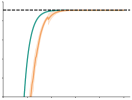
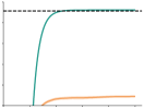
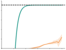
One-Way
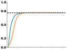
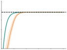
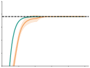
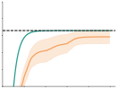
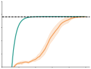
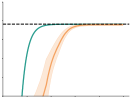
River Swim
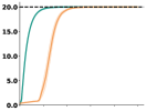
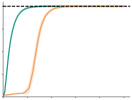
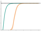
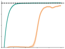
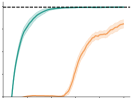
Loop
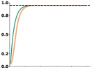
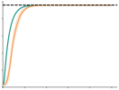
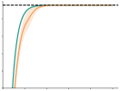
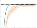
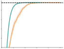
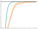
Corridor
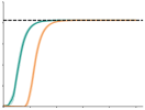
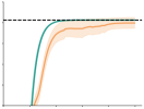
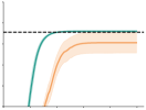
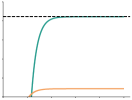
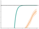
Two-Room-3x5
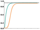
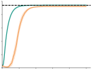
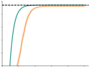
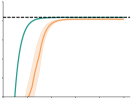
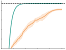
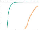
Two-Room-2x11
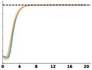
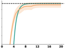
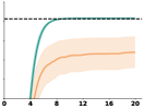
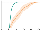
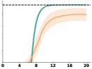
Training Steps ($\times 10^{3}$)

MDP

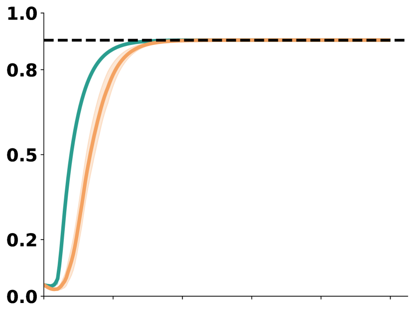
Semi-Random

Ask

Button

N-Supporters

Level Up

Figure 9: Monitored MBIE-EB comprehensively outperforms Directed-E². The y-axis represents the discounted test return. Solid lines are the average performance across 30 seeds. Shaded areas represent 95% confidence intervals.

B.4 When There Are Never-Observable Rewards

Mon-MDPs designed by Parisi et al. [2024a] do not have non-ergodic monitors, which give rise to unsolvable Mon-MDPs. Hence we introduce Bottleneck to investigate the performance of Monitored MBIE-EB compared to Directed-E².

As noted in footnote 8, Directed-E²’s performance in these settings depends critically on its reward model initialization. In order to see minimax-optimal performance from that algorithm, we need to initialize it pessimistically. Using the recommended random initialization saw essentially no learning in these domains. The algorithm would believe the never-observable rewards were at their initialized value, and so seek them out rather than treat their value pessimistically.

In Bottleneck the underlying reward of cells marked by $\bot$ is the same as being a snake (-10). In these experiments we use Full-Random monitor since it is more stochastic than Semi-Random to increase the challeng. Results are shown in Section G.2.1. The location of the button is chosen to test deep exploration capabilities of the agents to do a long sequence of costly actions in order to obtain the highest return. As a result the range of returns that the agent obtains with Button monitor is naturally lower than the rest of the Mon-MDPs.

One of the weaknesses of Directed-E² is the explicit dependency on the size of the state space in its objective. Since it tries to visit every joint state-action pair infinitely often without paying attention to their importance on maximizing the return, as the state space gets larger, the performance of Directed-E² deteriorates. To highlight this issue we use N-Experts monitor as an extension of Ask monitor; Ask is a special case when $N=1$. We see in Figure G.2.1 Directed-E²’s performance is hindered considerably when the agent faces N-Experts compared to Ask, while Monitored MBIE-EB suffers to a lesser degree.

Bottleneck
Training Steps ($\times 10^{3}$)

Full-Random

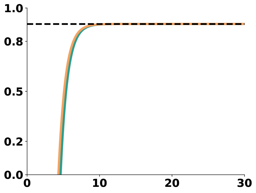
Ask

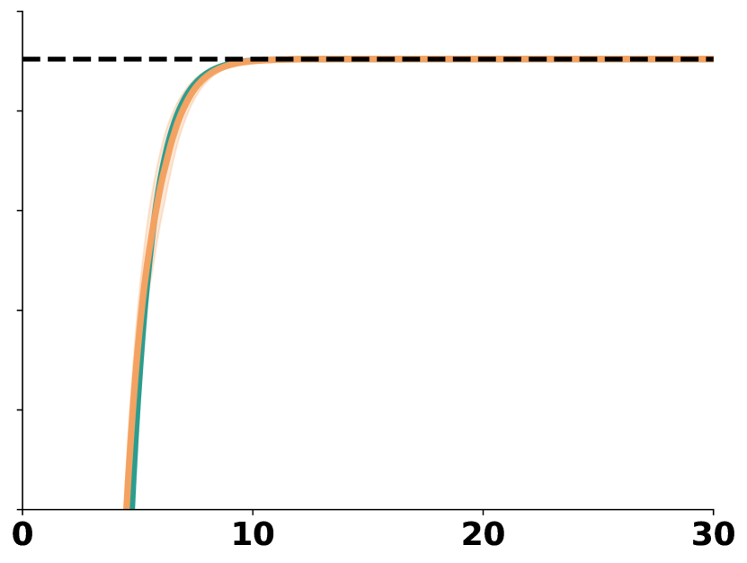
N-Supporters

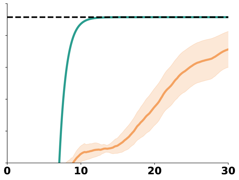
N-Experts

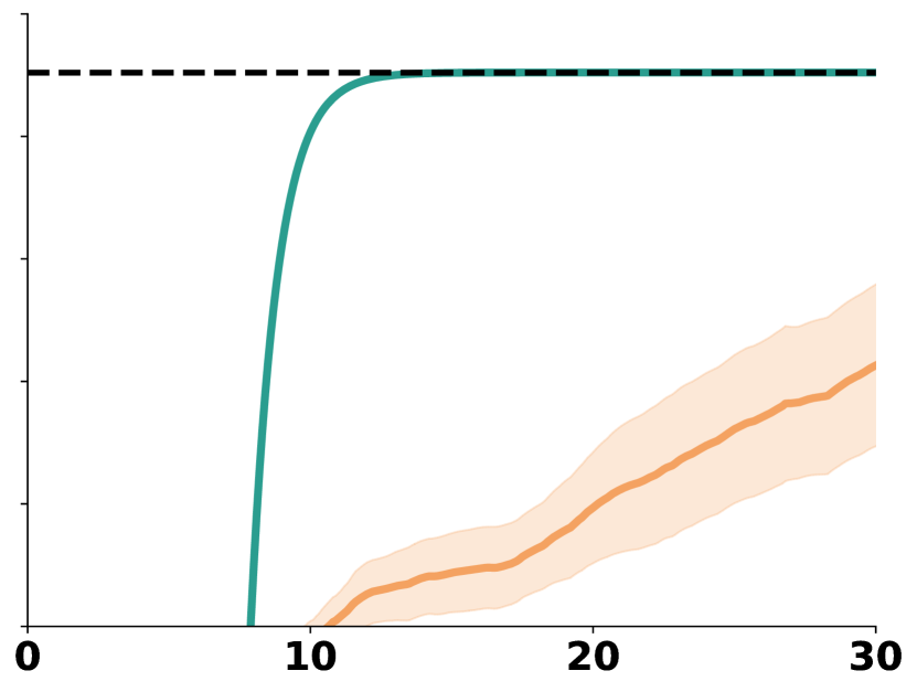
Level Up

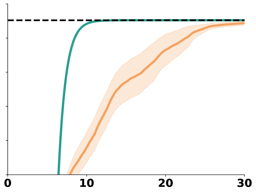
Button

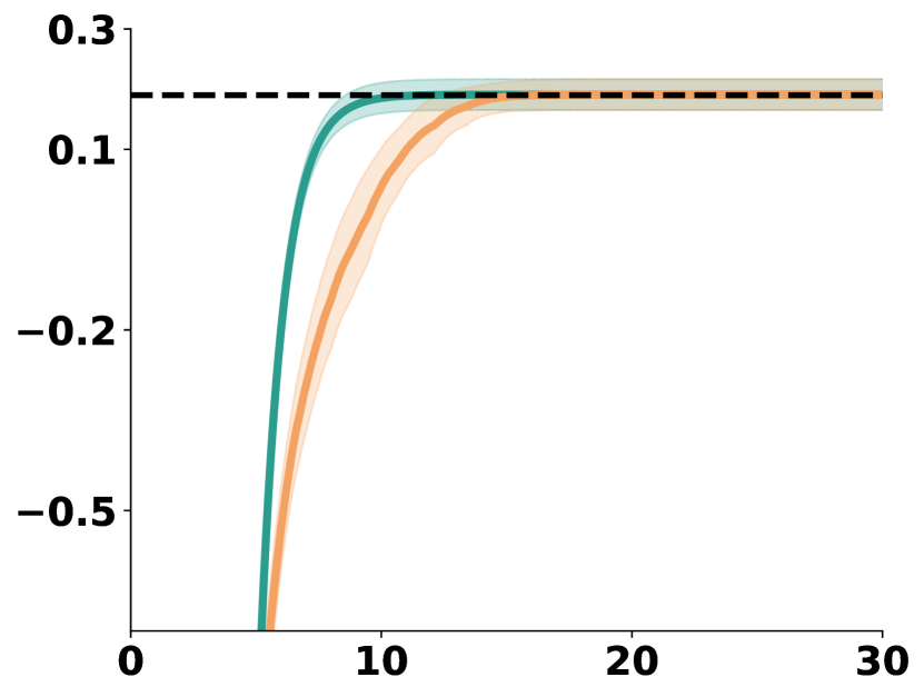
Figure 10: Monitored MBIE-EB outperforms Directed-E² on Bottleneck with non-ergodic monitor. The y-axis represents the discounted test return. Solid lines are the average performance across 30 seeds. Shaded areas represent 95% confidence intervals.

B.5 When There Are Stochastically-Observable Rewards

In all of the previous experiments had agent done the action that would have revealed the environment reward, such as asking in Ask monitor, by paying the cost it would have seen the reward with 100% certainty. But even if the probability is not 100% and yet bigger than 0, then upon enough attempts to observe the reward and paying the cost even if a portion of them are fruitless, it is possible to observe and learn the environment reward. In the following experiments, in addition to have environment state-action pairs that their reward is permanently unobservable, we make the monitor stochastic for other pairs such that even if the agent pays the cost, it would only observe the reward with probability $\rho$. In Figure 12, it can be seen that albeit the challenge of having stochastically and permanently unobservable rewards, Monitored MBIE-EB has not become prematurely pessimistic about the rewards that can be observed, even the probability goes down as low as 5%, and still outperforms Directed-E².

(80%)
(20%)
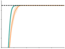
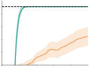
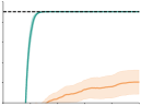
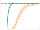
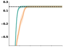
(5%)
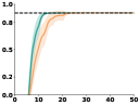
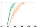
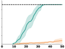
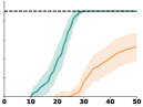
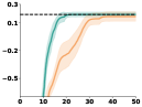
Training Steps ($\times 10^{3}$)

Full-Random

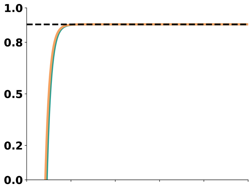
Ask

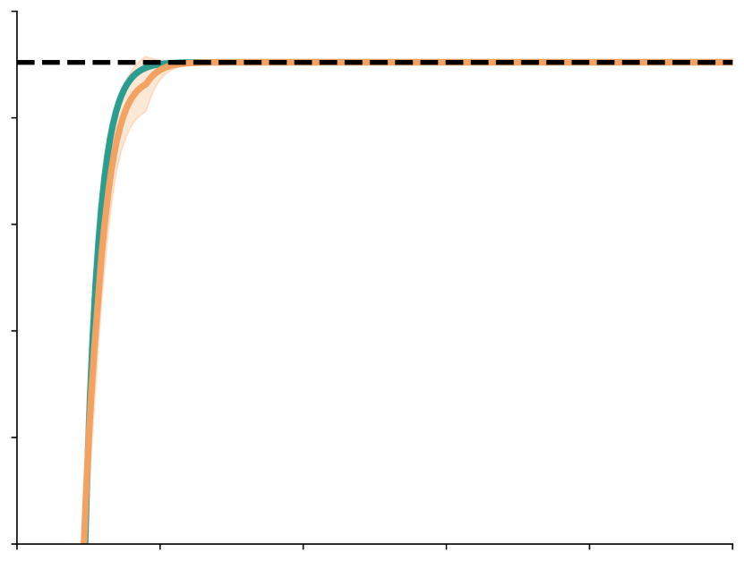
N-Supporters

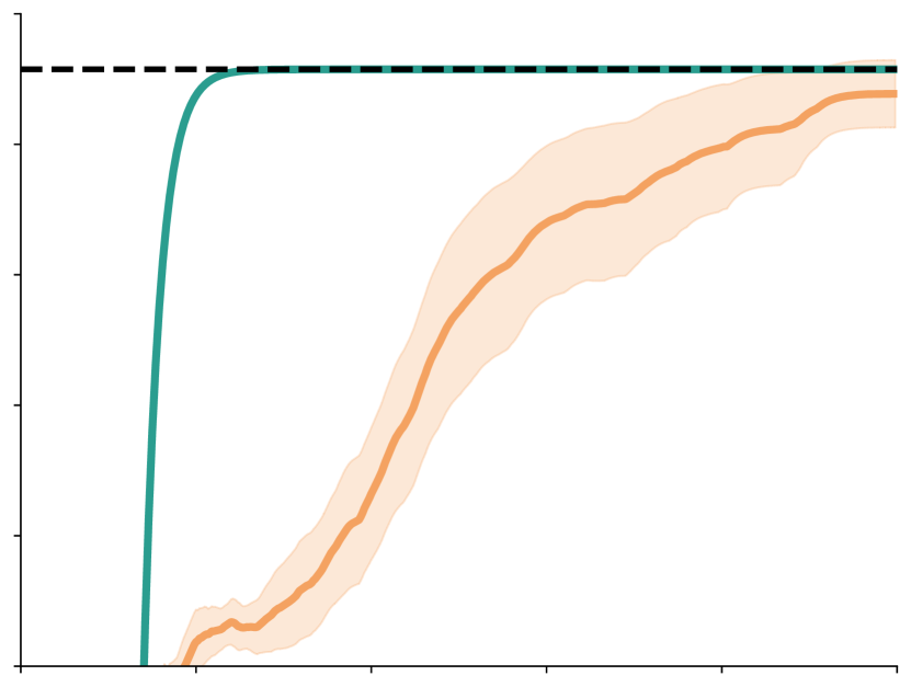
N-Experts

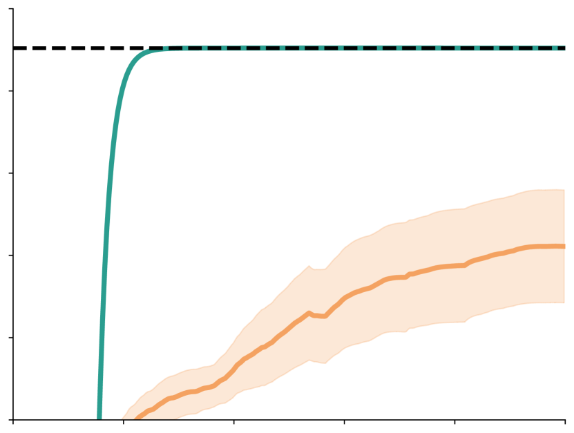
Level Up

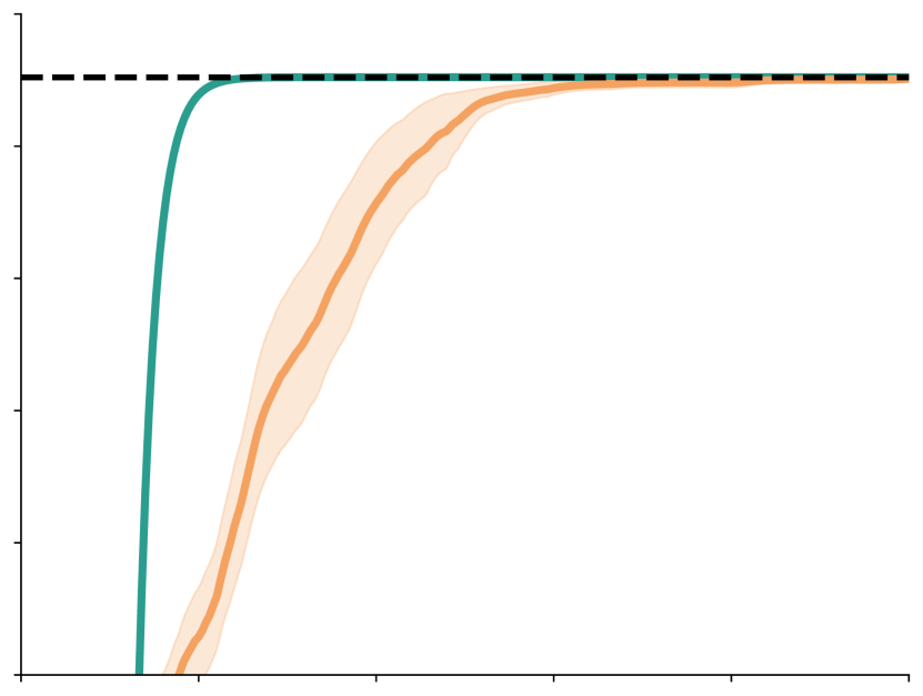
Button

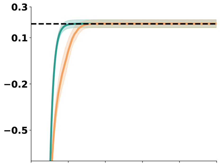
Figure 12: Monitored MBIE-EB outperforms Directed-E² even if environment rewards are stochastically observable. The y-axis represents the discounted test return. Solid lines are the average performance across 30 seeds. Shaded areas represent 95% confidence intervals.

B.6 When the Monitor is Known

We have shown the superior performance of Monitored MBIE-EB compared to Directed-E², now we investigate how much of the difficulty of learning in Mon-MDPs comes from the monitor being unknown. The unknown quantities of the monitor to the agent are $r^{\text{m}},P^{\text{m}}$, and $f^{\text{m}}$ so in the following experiments we make all of them known to the agent in advance. The only remaining unknown quantities are $r^{\text{e}}$ and $P^{\text{e}}$. So following the rationale of Section 3.1, it is enough to definite $\frac{\beta^{\text{e}}}{\sqrt{N(s^{\text{e}},a^{\text{e}})}}$ as the bonus for $R^{\text{e}}$, the same way it was defined before, and $\frac{\beta}{\sqrt{N(s^{\text{e}},a^{\text{e}})}}$ as the bonus for $P^{\text{e}}$ with the difference that in the latter $N(s^{\text{e}},a^{\text{e}})$ denotes the visitation count of $(s^{\text{e}},a^{\text{e}})$. Both of these bonuses should be used for $\bar{R}_{\text{optimize}}$, and $N(s^{\text{e}},a^{\text{e}})$ should be used for $\bar{R}_{\text{observe}}$ as well. Note that since the monitor is known there is no to use KL-UCB as the agent already know which rewards of which state-action pairs are observable (with what probability) and which ones are not.

As shown in Figure 14, the prior knowledge of the monitor’s quantities boosts the speed of Monitored MBIE-EB’s learning and make it substantially robust even in the low probability regimes.

(80%)
(20%)
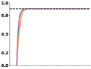
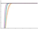
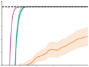
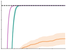
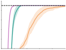
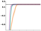
(5%)
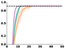
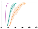
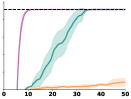
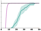
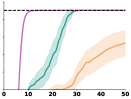
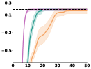
Training Steps ($\times 10^{3}$)

Full-Random

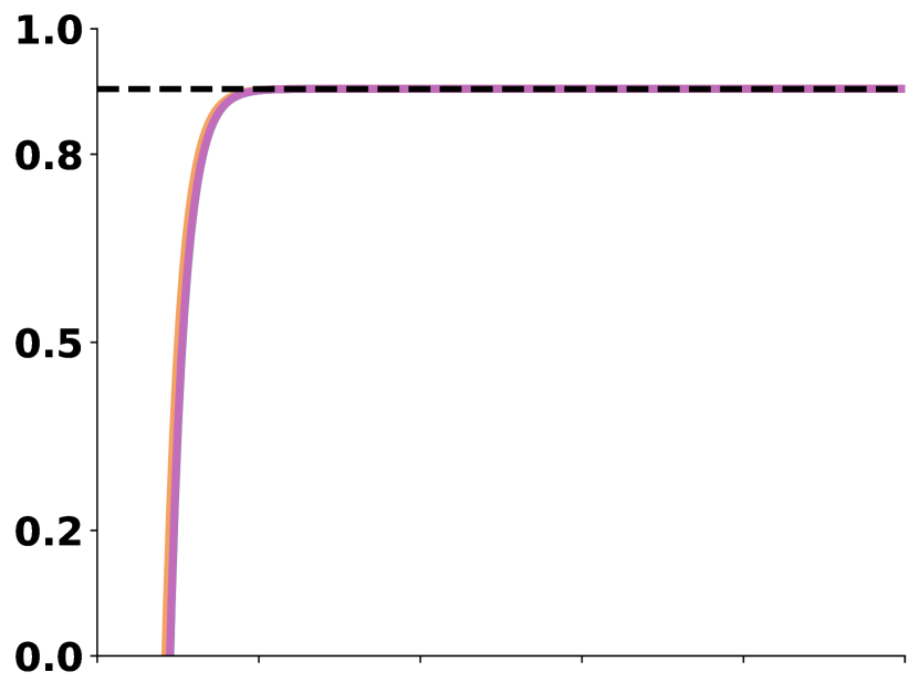
Ask

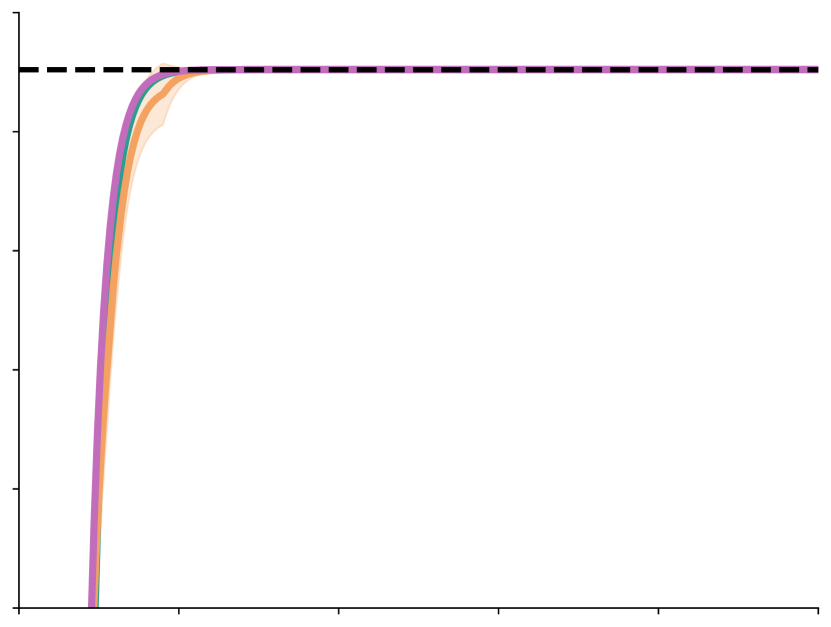
N-Supporters

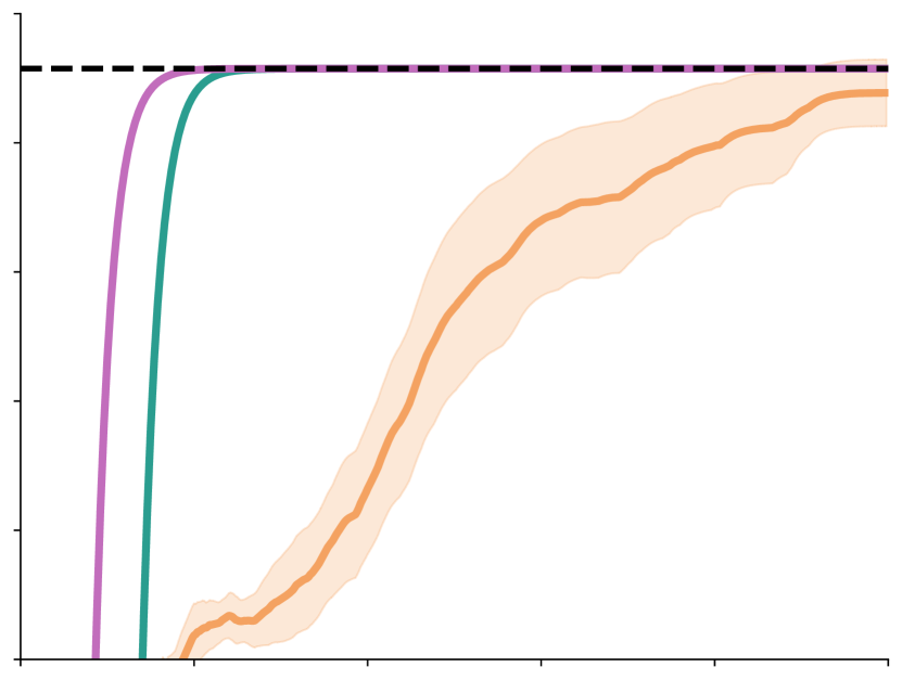
N-Experts

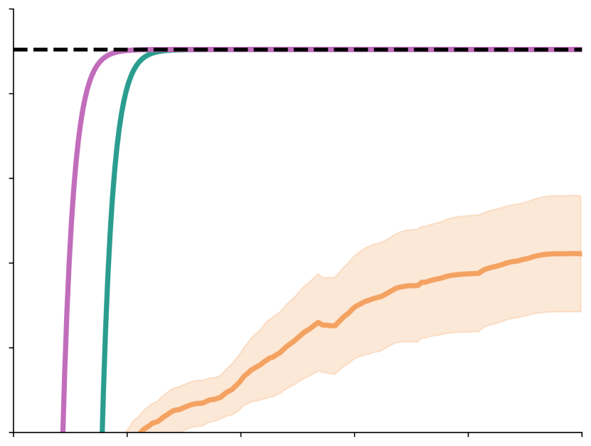
Level Up

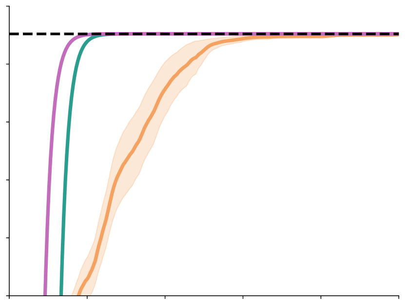
Button

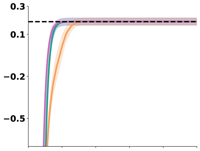
Figure 14: Knowing the monitor considerably accelerate learning in Mon-MDPs.The y-axis represents the discounted test return. Solid lines are the average performance across 30 seeds. Shaded areas represent 95% confidence intervals.

Appendix C Hyperparameters

Let $\mathcal{U}$ denote the uniform distribution and $x\mapsto y$ denote the linear annealing of a quantity taking initially the value of $x$ and ends with $y$.

Table 1: Hyperparameters of Monitored MBIE-EB across experiments.

Unknown monitor
Experiment	Environment	$\bar{Q}_{\text{optimize-init}}$	$\bar{Q}_{\text{observe-init}}$	$\kappa^{*}(k)$	$\beta^{\text{obs}}$	$\beta^{\text{KL-UCB}}$	$\beta$	$\beta^{\text{m}}$	$\beta^{\text{e}}$
Section B.3	Empty	1	100	$\log_{1.005}k$	$5\times 10^{-4}$	$5\times 10^{-2}$	$5\times 10^{-4}$	$5\times 10^{-4}$	$5\times 10^{-4}$
	Hazard	1	100	$\log_{1.005}k$	$5\times 10^{-4}$	$5\times 10^{-2}$	$5\times 10^{-4}$	$5\times 10^{-4}$	$5\times 10^{-4}$
	One-Way	1	100	$\log_{1.005}k$	$5\times 10^{-4}$	$5\times 10^{-2}$	$5\times 10^{-4}$	$5\times 10^{-4}$	$5\times 10^{-4}$
	River-Swim	30	100	$\log_{1.005}k$	$5\times 10^{-4}$	$5\times 10^{-2}$	$5\times 10^{-4}$	$5\times 10^{-4}$	$5\times 10^{-4}$
Section B.4	Bottleneck	1	100	$\log_{1.005}k$	$5\times 10^{-4}$	$5\times 10^{-2}$	$5\times 10^{-4}$	$5\times 10^{-4}$	$5\times 10^{-4}$
Section B.5	Bottleneck	1	100	$\log_{1.005}k$	$5\times 10^{-4}$	$5\times 10^{-2}$	$5\times 10^{-4}$	$5\times 10^{-4}$	$5\times 10^{-4}$
Appendix G	Bottleneck	50	100	$\log_{1.005}k$	$5\times 10^{-4}$	$5\times 10^{-2}$	$5\times 10^{-4}$	$5\times 10^{-4}$	$5\times 10^{-4}$

Known monitor
Experiment	Environment	$\bar{Q}_{\text{optimize-init}}$	$\bar{Q}_{\text{observe-init}}$	$\kappa^{*}(k)$	$\beta^{\text{e}}$	$\beta$
Section B.6	Bottleneck	1	100	$\log_{1.005}k$	$5\times 10^{-4}$	$5\times 10^{-4}$

Table 2: Hyperparameters of Directed-E² across experiments.

(Annealing for $N$-Supporters and $N$-Experts)
Experiment	Environment	$Q_{\text{int}}$	$S_{0}$	$r_{0}$	$\bar{\beta}$	$\upalpha$
Section B.3	Empty	-10	0	$\mathcal{U}[-0.1,0.1]$	$10^{-2}$	$1(1\mapsto 0.1)$
	One-Way	-10	0	$\mathcal{U}[-0.1,0.1]$	$10^{-2}$	$1(1\mapsto 0.1)$
	Hazard	-10	0	$\mathcal{U}[-0.1,0.1]$	$10^{-2}$	$0.5(0.5\mapsto 0.1)$
	River-Swim	-10	0	$\mathcal{U}[-0.1,0.1]$	$10^{-2}$	$0.5\mapsto 0.05$
Section B.5	Bottleneck	-10	0	$-10$	$10^{-2}$	$1(1\mapsto 0.1)$
Section B.5	Bottleneck	-10	0	$-10$	$10^{-2}$	$1(1\mapsto 0.1)$

C.1 Considerations

• Directed-E² uses two action-values, one as the ordinary action-values that uses a reward model in place of the environment reward to update action-values (this sets the agent free from the partial observability of the environment reward once the reward model is learned). Second action value function denoted by $S$ is dubbed as visitation-values that tries to maximized the successor representations. Directed-E² uses visitation-values to visit every joint state-action pairs but in the limit of infinite exploration it becomes greedy with respect to the main action-values for maximizing the expected sum of discounted rewards.

• Hyperparameters of Directed-E² consist of: $Q_{\text{int}}$ the initial action-values, $S_{0}$ the initial visitation-values, $r_{0}$ the initial values of the environment reward model, $\bar{\beta}$ goal-conditioned threshold specifying when a joint state-action pair should be visited through the use of visitation-values, $\upalpha$ the learning rate to update each $Q$ or $S$ incrementally and discount factor $\gamma$ that is held fixed $0.99$. These values are directly reported from Parisi et al. [2024a].

• Monitored MBIE-EB’s hyperparameters are set per environment and do not change across monitors. The same applies to Directed-E², but Parisi et al. [2024a] recommend to tune an ad-hoc learning rate once N-Supporters or N-Experts are used as monitors.

• In experiments ofSection B.5, observability is stochastic thus we make $\kappa^{*}(k)$ grow slowly. This makes the agent spend time more frequently at the observe episodes to deal with low probability of 5% for observing the reward more aggressively. Even if in higher probabilities of 20% and 80% faster rates for $\kappa^{*}(k)$ are also applicable we kept $\kappa^{*}(k)$ universal for those experiments.

• KL-UCB does not have a closed form solution, we compute it using the Newton’s method. The stopping condition for the Newton’s method is chosen 50 iterations or the accuracy of at least $10^{-5}$ between successive iterative solutions, which one happens first.

• Due to knowledge of the monitor, agent should would not need to spend a lot of time in the observe episodes, although probability of observing the reward could go as low as $5\%$, we set the $\kappa^{*}(k)$ with faster rate than when the monitor is unknown. Due to this agent wastes less of its efforts in the observe episodes.

Appendix D Compute

We ran all experiments on a SLURM-based cluster, using 32 Intel E5-2683 v4 Broadwell @ 2.1GHz CPUs. 30 runs took about an hour on a 32 core CPU. Runs were parallelized whenever possible across cores.

Appendix E Propositions

Lemma E.1.

For any $a,x>0$, $x\geq 2a\ln{a}$ implies $x\geq a\ln{x}$.

Proof.

First we prove that for $\forall x>0$, $x>2\ln{x}$.

Consider the function $y=x-2\ln{x}$. It is enough to prove that $y>0$ is always true on its domain. we have that

$$\frac{dy}{dx}=1-\frac{2}{x}$$

$$\frac{d^{2}y}{d^{2}x}=\frac{2}{x^{2}}>0$$

So $y=x-\ln{x}$ is convex. Also by:

$$\frac{dy}{dx}=1-\frac{2}{x}=0\Rightarrow x=2$$

The minimum of $y=x-\ln{x}=2-\ln{2}>0$. Thus $x>2\ln{x},\forall x>0$.

Back to the inequalities in the lemma, let $z=\frac{x}{a}$, then we need to prove that $z\geq 2\ln{a}$ implies $z\geq\ln{(za)}$.

• If $a\geq z$, then:

  $$\ln{za}=\ln{z}+\ln{a}\leq 2\ln{a}\leq z$$

  Which is by the assumption of $z\geq 2\ln{a}$.

• If $a<z$, then:

  $$\ln{a}<\ln{z}\Rightarrow\ln{za}\leq 2\ln{z}<z$$

  which is by our proof in the beginning that $z\geq 2\ln{z},\forall z>0$. ∎

Lemma E.2.

Let $\Omega$ be an outcome space, and each of $(A_{i})^{n}_{i=1}$ and $(B_{i})^{n}_{i=1}$ be $n$ random variables on $\Omega$. It holds that:

$$\left\{\sum_{i=1}^{n}A_{i}\geq\sum_{i=1}^{n}B_{i}\right\}\subseteq\left\{\bigcup^{n}_{i=1}(A_{i}\geq B_{i})\right\}$$

Proof.

Proof by contradiction.

Suppose $\left\{\sum_{i=1}^{n}A_{i}\geq\sum_{i=1}^{n}B_{i}\right\}\supset\left\{\bigcup^{n}_{i=1}(A_{i}\geq B_{i})\right\}$, then it means there exists an $\omega\in\Omega$ such that $\sum_{i=1}^{n}A_{i}(\omega)\geq\sum_{i=1}^{n}B_{i}(\omega)$ but $A_{1}(\omega)<B_{1}(\omega),A_{2}(\omega)<B_{2}(\omega),\cdots A_{n}(\omega)<B_{n}(\omega)$ that results in $\sum_{i=1}^{n}A_{i}(\omega)<\sum_{i=1}^{n}B_{i}(\omega)$ which is a contradiction. ∎

Corollary E.3.

Let $(A_{i})^{n}_{i=1}$ and $(B_{i})^{n}_{i=1}$ be $n$ random variables on probability space $(\Omega,\mathcal{F},\mathbb{P})$. It holds that:

$$\mathbb{P}\left[{\sum_{i=1}^{n}A_{i}\geq\sum_{i=1}^{n}B_{i}}\right]\leq\sum_{i=1}^{n}\mathbb{P}\left[{A_{i}\geq B_{i}}\right]$$

Proof.

Using Lemma E.2 and due to monotonicity of measures we have:

$$\mathbb{P}\left[{\sum_{i=1}^{n}A_{i}\geq\sum_{i=1}^{n}B_{i}}\right]\leq\mathbb{P}\left[{\bigcup^{n}_{i=1}(A_{i}\geq B_{i})}\right]$$

By applying the union bound the inequality is obtained. ∎

Lemma E.4.

Let $M_{1}=\left\langle\mathcal{S},\mathcal{A},P_{1},r_{1},f^{\text{m}},\gamma\right\rangle$ and $M_{2}=\left\langle\mathcal{S},\mathcal{A},P_{2},r_{2},f^{\text{m}},\gamma\right\rangle$ be two Mon-MDPs where $r_{1}=(r^{\text{e}}_{1},r^{\text{m}}_{1})$, $R_{2}=(r^{\text{e}}_{2},r^{\text{m}}_{2})$. Assume the following bounds hold:

$$-r_{\text{max}}^{\text{e}}\leq r^{\text{e}}_{1},r^{\text{e}}_{2}\leq r_{\text{max}}^{\text{e}}\text{ and }-r_{\text{max}}^{\text{m}}\leq r^{\text{m}}_{1},r^{\text{m}}_{2}\leq r_{\text{max}}^{\text{m}}$$

Additionally assume the following conditions hold for all joint state-action pairs $(s,a)\equiv(s^{\text{e}},s^{\text{m}},a^{\text{e}},a^{\text{m}})$:

$$\left\lvert r^{\text{e}}_{1}(s^{\text{e}},a^{\text{e}})-r^{\text{e}}_{2}(s^{\text{e}},a^{\text{e}})\right\rvert \leq\varphi^{\text{e}}$$

$$\left\lvert r^{\text{m}}_{1}(s^{\text{m}},a^{\text{m}})-r^{\text{m}}_{2}(s^{\text{m}},a^{\text{m}})\right\rvert \leq\varphi^{\text{m}}$$

$$\left\lVert P_{1}(\cdot\mid s,a)-P_{2}(\cdot\mid s,a)\right\rVert_{1} \leq\varphi$$

then for any stationary deterministic policies $\pi$ it holds that:

$$\left\lvert Q^{M_{1}}_{\pi}(s,a)-Q^{M_{2}}_{\pi}(s,a)\right\rvert\leq\frac{\varphi^{\text{e}}+\varphi^{\text{m}}+2\varphi\gamma(r_{\text{max}}^{\text{e}}+r_{\text{max}}^{\text{m}})}{(1-\gamma)^{2}}$$

Proof.

Let
$\Delta\coloneqq\max_{(s,a)}\left\lvert Q^{M_{1}}_{\pi}(s,a)-Q^{M_{2}}_{\pi}(s,a)\right\rvert,\\ \Delta_{1}\coloneqq r^{\text{e}}_{1}(s^{\text{e}},a^{\text{e}})-r^{\text{e}}_{2}(s^{\text{e}},a^{\text{e}}),\\ \Delta_{2}\coloneqq r^{\text{m}}_{1}(s^{\text{m}},a^{\text{m}})-r^{\text{m}}_{2}(s^{\text{m}},a^{\text{m}})$ and
$\Delta_{3}\coloneqq\gamma\sum_{s^{\prime}}P_{1}(s^{\prime}\mid s,a)V^{M_{1}}_{\pi}(s^{\prime})-\gamma\sum_{s^{\prime}}P_{2}(s^{\prime}\mid s,a)V^{M_{2}}_{\pi}(s^{\prime})$.

Then:

$$\left\lvert Q^{M_{1}}_{\pi}(s,a)-Q^{M_{2}}_{\pi}(s,a)\right\rvert=\left\lvert\Delta_{1}+\Delta_{2}+\Delta_{3}\right\rvert\leq\left\lvert\Delta_{1}\right\rvert+\left\lvert\Delta_{2}\right\rvert+\left\lvert\Delta_{3}\right\rvert$$

$$\leq\varphi^{\text{e}}+\varphi^{\text{m}}+\gamma\left\lvert\sum_{s^{\prime}}\left(P_{1}(s^{\prime}\mid s,a)V^{M_{1}}_{\pi}(s^{\prime})-P_{2}(s^{\prime}\mid s,a)V^{M_{2}}_{\pi}(s^{\prime})\right)\right\rvert$$

$$=\varphi^{\text{e}}+\varphi^{\text{m}}+\gamma\left\lvert\sum_{s^{\prime}}\left(P_{1}(s^{\prime}\mid s,a)V^{M_{1}}_{\pi}(s^{\prime})-P_{1}(s^{\prime}\mid s,a)V^{M_{2}}_{\pi}(s^{\prime})+P_{1}(s^{\prime}\mid s,a)V^{M_{2}}_{\pi}(s^{\prime})-P_{2}(s^{\prime}\mid s,a)V^{M_{2}}_{\pi}(s^{\prime})\right)\right\rvert$$

$$=\varphi^{\text{e}}+\varphi^{\text{m}}+\gamma\left\lvert\sum_{s^{\prime}}\left(P_{1}(s^{\prime}\mid s,a)\left(V^{M_{1}}_{\pi}(s^{\prime})-V^{M_{2}}_{\pi}(s^{\prime})\right)+\left(P_{1}(s^{\prime}\mid s,a)-P_{2}(s^{\prime}\mid s,a)\right)V^{M_{2}}_{\pi}(s^{\prime})\right)\right\rvert$$

$$\leq\varphi^{\text{e}}+\varphi^{\text{m}}+\gamma\left\lvert\sum_{s^{\prime}}P_{1}(s^{\prime}\mid s,a)\left(V^{M_{1}}_{\pi}(s^{\prime})-V^{M_{2}}_{\pi}(s^{\prime})\right)\right\rvert+\gamma\left\lvert\sum_{s^{\prime}}\left(P_{1}(s^{\prime}\mid s,a)-P_{2}(s^{\prime}\mid s,a)\right)V^{M_{2}}_{\pi}(s^{\prime})\right\rvert$$

$$\leq\varphi^{\text{e}}+\varphi^{\text{m}}+\gamma\left\lvert\sum_{s^{\prime}}P_{1}(s^{\prime}\mid s,a)\left(V^{M_{1}}_{\pi}(s^{\prime})-V^{M_{2}}_{\pi}(s^{\prime})\right)\right\rvert+\frac{2\gamma\varphi\left(r_{\text{max}}^{\text{e}}+r_{\text{max}}^{\text{m}}\right)}{1-\gamma}$$

By taking the $\max_{(s,a)}$ from the both sides we have:

$$\Delta \leq\varphi^{\text{e}}+\varphi^{\text{m}}+\gamma\Delta+\frac{2\gamma\varphi\left(r_{\text{max}}^{\text{e}}+r_{\text{max}}^{\text{m}}\right)}{1-\gamma}$$

$$(1-\gamma)\Delta \leq\varphi^{\text{e}}+\varphi^{\text{m}}+\frac{2\gamma\varphi\left(r_{\text{max}}^{\text{e}}+r_{\text{max}}^{\text{m}}\right)}{1-\gamma}$$

$$\Delta \leq\frac{\varphi^{\text{e}}+\varphi^{\text{m}}}{1-\gamma}+\frac{2\gamma\varphi\left(r_{\text{max}}^{\text{e}}+r_{\text{max}}^{\text{m}}\right)}{(1-\gamma)^{2}}$$

$$\Delta \leq\frac{\varphi^{\text{e}}+\varphi^{\text{m}}+2\gamma\varphi(r_{\text{max}}^{\text{e}}+r_{\text{max}}^{\text{m}})}{(1-\gamma)^{2}}$$

And since $\left\lvert Q^{M_{1}}_{\pi}(s,a)-Q^{M_{2}}_{\pi}(s,a)\right\rvert\leq\Delta$, the proof is completed. ∎

For the following lemma without loss of generality assume $r_{\text{max}}^{\text{e}}=r_{\text{max}}^{\text{m}}=1$.

Lemma E.5.

Let $M_{1}=\left\langle\mathcal{S},\mathcal{A},P_{1},r_{1},f^{\text{m}},\gamma\right\rangle$ and $M_{2}=\left\langle\mathcal{S},\mathcal{A},P_{2},r_{2},f^{\text{m}},\gamma\right\rangle$ be two Mon-MDPs where $r_{1}=(r^{\text{e}}_{1},r^{\text{m}}_{1})$, $r_{2}=(r^{\text{e}}_{2},r^{\text{m}}_{2})$. Assume the following bounds hold:

$$-r_{\text{max}}^{\text{e}}\leq r^{\text{e}}_{1},r^{\text{e}}_{2}\leq r_{\text{max}}^{\text{e}}\text{ and }-r_{\text{max}}^{\text{m}}\leq r^{\text{m}}_{1},r^{\text{m}}_{2}\leq r_{\text{max}}^{\text{m}}$$

Suppose further that for all joint state-action pairs $(s,a)\equiv(s^{\text{e}},s^{\text{m}},a^{\text{e}},a^{\text{m}})$ the following conditions are satisfied:

$$\left\lvert r^{\text{e}}_{1}(s^{\text{e}},a^{\text{e}})-r^{\text{e}}_{2}(s^{\text{e}},a^{\text{e}})\right\rvert \leq\varphi^{\text{e}}$$

$$\left\lvert r^{\text{m}}_{1}(s^{\text{m}},a^{\text{m}})-r^{\text{m}}_{2}(s^{\text{m}},a^{\text{m}})\right\rvert \leq\varphi^{\text{m}}$$

$$\left\lVert P_{1}(\cdot\mid s,a)-P_{2}(\cdot\mid s,a)\right\rVert_{1} \leq\varphi$$

There exists a constant $C$ such that for any $0\leq\varepsilon\leq\nicefrac{{(r_{\text{max}}^{\text{e}}+r_{\text{max}}^{\text{m}})}}{{1-\gamma}}$, and any stationary policy $\pi$, if $\varphi^{\text{e}}=\varphi^{\text{m}}=\varphi=C\frac{\varepsilon(1-\gamma)^{2}}{r_{\text{max}}^{\text{e}}+r_{\text{max}}^{\text{m}}}$, then

$$\left\lvert Q^{M_{1}}_{\pi}(s,a)-Q^{M_{2}}_{\pi}(s,a)\right\rvert\leq\varepsilon$$

Proof.

Using Lemma E.4, we should show that:

$$\frac{\varphi^{\text{e}}+\varphi^{\text{m}}+2\varphi\gamma(r_{\text{max}}^{\text{e}}+r_{\text{max}}^{\text{m}})}{(1-\gamma)^{2}}=2\varphi\frac{1+\gamma(r_{\text{max}}^{\text{e}}+r_{\text{max}}^{\text{m}})}{(1-\gamma)^{2}}\leq\varepsilon$$

which yields:

$$\varphi\leq\frac{\varepsilon(1-\gamma)^{2}}{2\left(1+\gamma(r_{\text{max}}^{\text{e}}+r_{\text{max}}^{\text{m}})\right)}$$

And by our assumption that $r_{\text{max}}^{\text{e}}=r_{\text{max}}^{\text{m}}=1$:

$$\varphi\leq\frac{\varepsilon(1-\gamma)^{2}}{6(r_{\text{max}}^{\text{e}}+r_{\text{max}}^{\text{m}})}$$

By choosing $C=6$ the proof is completed. ∎

Lemma E.6 (Chernoff-Hoeffding’s inequality).

For $(V_{i})_{i=1}^{n}$ independent samples on probability space $(\Omega,\mathcal{F},\mathbb{P})$ where $V_{i}\in[a_{i},b_{i}]$ for all $i$ and $\epsilon>0$, we have:

$$\mathbb{P}\left[{\mathbb{E}\left[{V_{1}}\right]-\frac{1}{n}\sum_{i=1}^{n}V_{i}\geq\epsilon}\right]\leq\exp{\left(-\frac{2n^{2}\epsilon^{2}}{\sum_{i=1}^{n}(b_{i}-a_{i})^{2}}\right)}$$

Appendix F Proof of Theorem 3.1

We present the proof in 5 stages, each holds with high probability.

1. Specifying the number of samples required to estimate the observability of the environment reward in observe episodes

2. Optimism of $\bar{Q}_{*,\text{observe}}$

3. Specifying the number of samples required to find a near minimax optimal policy in optimize episodes

4. Optimism of $\bar{Q}_{*,\text{optimize}}$

5. Determining the sample complexity

For the first 2 stage of the proof let $b(s,a)=\mathbb{E}\left[{\mathds{1}\scriptstyle{\{\widehat{R}^{\text{e}}(s,a)\neq 0\}}}\right]$ denote the expected observability of the environment reward for the joint state-action $(s,a)$. And define $\tilde{B}$ to be the maximum likelihood estimation of $b$.

1. Specifying the number of samples required to estimate the observability of reward in observe episodes.

According to Lemma 2 of Strehl and Littman [2008], to find a policy in observation episodes that its action-values, computed using $\tilde{B}$ and $\tilde{P}$, are $\varepsilon_{1}$-close to their true values, $\tilde{B}$ and $\tilde{P}$ should be $\tau$-close to their true mean for all states $s$ and actions $a$ where $\tau=\varepsilon_{1}(1-\gamma)^{2}\big{/}2$. So in order to specify the least number of visits $m_{1}$ to $(s,a)$ to fulfill the $\tau$-closeness:

$$\begin{split}\left\lVert\tilde{P}(\cdot\mid s,a)-P(\cdot\mid s,a)\right\rVert_{1}&\leq\tau\end{split}$$ (14)

$$\begin{split}\left\lvert\tilde{B}(s,a)-b(s,a)\right\rvert&\leq\tau\end{split}$$ (15)

On the other hand we know if $(s,a)$ has been visited $m_{1}$ times, with probabilities at least $1-\delta_{P}$, and $1-\delta_{B}$:

$$\left\lVert\tilde{P}(\cdot\mid s,a)-P(\cdot\mid s,a)\right\rVert_{1} \leq\sqrt{\frac{2\left[\ln{(2^{|\mathcal{S}|}-2)-\ln{\delta_{P}}}\right]}{m_{1}}}$$

$$\left\lvert\tilde{B}(s,a)-b(s,a)\right\rvert \leq\sqrt{\frac{\ln{\nicefrac{{2}}{{\delta_{B}}}}}{2m_{1}}}$$

So for Equation 14 and Equation 15 to hold simultaneously with probability at $1-\delta_{1}$ until $(s,a)$ is visited $m_{1}$ times, by setting $\delta_{p}=\delta_{B}=\delta_{1}\big{/}2\left\lvert\mathcal{S}\right\rvert\left\lvert\mathcal{A}\right\rvert m_{1}$ to split the failure probability equally for all state-action pairs until each of them have been visited $m_{1}$ times, it is enough ensure $\tau$ is bigger than the length of the confidence intervals, so:

$$m_{1} \geq\max\left\{\frac{8\left[\ln{(2^{\left\lvert\mathcal{S}\right\rvert}-2)-\ln{\delta_{P}}}\right]}{\tau^{2}},\frac{2\ln{\nicefrac{{2}}{{\delta_{B}}}}}{\tau^{2}}\right\}$$

$$\geq\max\left\{\frac{8\left[\ln{(2^{\left\lvert\mathcal{S}\right\rvert}-2)-\ln{\nicefrac{{\delta_{1}}}{{2\left\lvert\mathcal{S}\right\rvert\left\lvert\mathcal{A}\right\rvert m_{1}}}}}\right]}{\tau^{2}},\frac{2\ln{\nicefrac{{4\left\lvert\mathcal{S}\right\rvert\left\lvert\mathcal{A}\right\rvert m_{1}}}{{\delta_{1}}}}}{\tau^{2}}\right\}$$

$$=\frac{8\left[\ln{(2^{|\mathcal{S}|}-2)+\ln{\nicefrac{{2\left\lvert\mathcal{S}\right\rvert\left\lvert\mathcal{A}\right\rvert m_{1}}}{{\delta_{1}}}}}\right]}{\tau^{2}}$$

Lemma E.1 helps us to bring $m_{1}$ out of the right-hand side of the above inequality. Hence:

$$m_{1}=\mathcal{O}\left(\frac{\left\lvert\mathcal{S}\right\rvert}{\tau^{2}}+\frac{1}{\tau^{2}}\ln{\frac{\left\lvert\mathcal{S}\right\rvert\left\lvert\mathcal{A}\right\rvert}{\tau\delta_{1}}}\right)=\mathcal{O}\left(\frac{|\mathcal{S}|}{\varepsilon_{1}^{2}(1-\gamma)^{4}}+\frac{1}{\varepsilon_{1}^{2}(1-\gamma)^{4}}\ln{\frac{\left\lvert\mathcal{S}\right\rvert\left\lvert\mathcal{A}\right\rvert}{\varepsilon_{1}(1-\gamma)^{2}\delta_{1}}}\right)$$

The bound shows the fact that regardless of how infinitesimal the probability of observing the reward is, the difficulty of learning good estimates lies in learning the transition dynamics [Kakade, 2003, Szita and Szepesvári, 2010]; by the time that the transition dynamics are approximately learned, the agent has approximately figured out the what the probability of observing the environment reward for taking any joint action is.

2. Optimism of $\bar{Q}_{*,\text{observe}}$.

Optimism is needed to make sure the agent has enough incentives to visit state-action pairs that their statistics are not close enough to their true values. Suppose $m_{1}$ is least number of samples required to ensure $\tilde{B}$ and $\tilde{P}$ are close to their true mean. Then the agent should be optimistic about the action-values of state-action pairs that have not been visited $m_{1}$ times so far.

Let:

$$Q_{*,\text{observe}}(s,a)=b(s,a)\mathds{1}\{N(s^{\text{e}},a^{\text{e}})=0\}+\gamma\sum_{s^{\prime}}P(s^{\prime}\mid s,a)\max_{a^{\prime}}Q_{\text{*, \text{observe}}}(s^{\prime},a^{\prime})$$

Now consider the first $v$ visits to $(s,a)$ during observation episodes, where $v<m_{1}$ and the corresponding action values:

$$\bar{Q}_{*,\text{observe}}(s,a)=\tilde{B}(s,a)\mathds{1}\{N(s^{\text{e}},a^{\text{e}})=0\}+\gamma\sum_{s^{\prime}}\tilde{P}(s^{\prime}\mid s,a)\max_{a^{\prime}}\bar{Q}_{*,\text{observe}}(s^{\prime},a^{\prime})+\frac{\beta^{\text{obs}}}{\sqrt{v}}$$ (16)

$\tilde{B}(s,a)\mathds{1}\{N(s^{\text{e}},a^{\text{e}})=0\}=0$ for all state-action pairs. Because if $\mathds{1}\{N(s^{\text{e}},a^{\text{e}})=0\}$ returns 1, then it means environment reward of $(s,a)$ has not been observed so far and $\tilde{B}(s,a)=0$. So Equation 16 turns into:

$$\bar{Q}_{*,\text{observe}}(s,a)=\gamma\sum_{s^{\prime}}\tilde{P}(s^{\prime}\mid s,a)\max_{a^{\prime}}\bar{Q}_{*,\text{observe}}(s^{\prime},a^{\prime})+\frac{\beta^{\text{obs}}}{\sqrt{v}}$$ (17)

According to Lemma 7 of Strehl and Littman [2008], by choosing $\beta^{\text{obs}}=\left({1}\big{/}{(1-\gamma)}\sqrt{\ln{\left(\nicefrac{{4\left\lvert\mathcal{S}\right\rvert\left\lvert\mathcal{A}\right\rvert m_{1}}}{{\delta_{1}}}\right)}\big{/}{2}}\right)$:

$$\bar{Q}_{*,\text{observe}}(s,a)=\gamma\sum_{s^{\prime}}\tilde{P}(s^{\prime}\mid s,a)\max_{a^{\prime}}\bar{Q}_{*,\text{observe}}(s^{\prime},a^{\prime})+\frac{\beta^{\text{obs}}}{\sqrt{v}}\geq Q_{*,\text{observe}}(s,a)$$

with probability at least $1-{\delta_{1}}\big{/}{4\left\lvert\mathcal{S}\right\rvert\left\lvert\mathcal{A}\right\rvert m_{1}}$. On the other hand by choosing $\beta^{\text{KL-UCB}}=\ln(4\left\lvert\mathcal{S}\right\rvert\left\lvert\mathcal{A}\right\rvert m_{1}\big{/}\delta_{1})$:

$$\text{KL-UCB}(v)=\max\{\mu\in[0,1]:d(0,\mu)\leq\frac{\beta^{\text{KL-UCB}}}{v}\}\geq b(s,a)\mathds{1}\{N(s^{\text{e}},a^{\text{e}})=0\}$$

holds with probability at least $1-{\delta_{1}}\big{/}{4\left\lvert\mathcal{S}\right\rvert\left\lvert\mathcal{A}\right\rvert m_{1}}$, where $d$ is the relative entropy distance appropriate for building the confidence interval of Bernoulli random variables [Lattimore and Szepesvári, 2020, Garivier and Cappé, 2011, Maillard et al., 2011].

Now consider the following random variables:

$$X=Q_{*,\text{observe}}(s,a)-\gamma\sum_{s^{\prime}}\tilde{P}(s^{\prime}\mid s,a)\max_{a^{\prime}}\bar{Q}_{*,\text{observe}}(s^{\prime},a^{\prime}), Y=\tilde{B}(s,a)\mathds{1}\{N(s^{\text{e}},a^{\text{e}})=0\}=0$$

We have that:

$$\mathbb{P}\left[{X\geq\underbrace{\frac{\beta^{\text{obs}}}{\sqrt{v}}}_{B_{1}}}\right]\leq\frac{\delta_{1}}{4\left\lvert\mathcal{S}\right\rvert\left\lvert\mathcal{A}\right\rvert m_{1}}, \mathbb{P}\left[{Y\geq\underbrace{\max\left\{\mu\in[0,1]:d(0,\mu)\leq\frac{\beta^{\text{KL-UCB}}}{v}\right\}}_{B_{2}}}\right]\leq\frac{\delta_{1}}{4\left\lvert\mathcal{S}\right\rvert\left\lvert\mathcal{A}\right\rvert m_{1}}$$

Using Corollary E.3 we have:

$$\mathbb{P}\left[{X+Y\geq B_{1}+B_{2}}\right]\leq\frac{\delta_{1}}{2\left\lvert\mathcal{S}\right\rvert\left\lvert\mathcal{A}\right\rvert m_{1}}$$

Thus with probability at least $1-{\delta_{1}}\big{/}{2\left\lvert\mathcal{S}\right\rvert\left\lvert\mathcal{A}\right\rvert m_{1}}$ we must have that $X+Y\leq B_{1}+B_{2}$. By replacing the explicit values of $X$ and $Y$, we have:

$$Q_{*,\text{observe}}(s,a)-\gamma\sum_{s^{\prime}}\tilde{P}(s^{\prime}\mid s,a)\max_{a^{\prime}}\bar{Q}_{*,\text{observe}}(s^{\prime},a^{\prime})\leq B_{1}+B_{2}$$

$$Q_{*,\text{observe}}(s,a)\leq\gamma\sum_{s^{\prime}}\tilde{P}(s^{\prime}\mid s,a)\max_{a^{\prime}}\bar{Q}_{*,\text{observe}}(s^{\prime},a^{\prime})+B_{1}+B_{2}$$

$$Q_{*,\text{observe}}(s,a)\leq\bar{Q}_{*,\text{observe}}(s,a)+\max\left\{\mu\in[0,1]:d(0,\mu)\leq\frac{\beta^{\text{KL-UCB}}}{v}\right\}$$

And by abusing the notation for $\bar{Q}_{*,\text{observe}}$ to incorporate the KL-UCB term, we have:

$$Q_{*,\text{observe}}(s,a)\leq\bar{Q}_{*,\text{observe}}(s,a)$$

By using the union bound over $\mathcal{S},\mathcal{A}$ and $m_{1}$ the above inequality holds for all state-action pairs until they are visited $m_{1}$ times with probability at least $1-\frac{\delta_{1}}{2}$.

3. Specifying the number of samples required to find a near minimax optimal policy in optimize episodes.

During optimize episodes agent can face two kinds of joint state-action pairs: 1) state-action pairs that lead to observing the environment reward e.g., moving and asking for reward 2) state -action pairs that do not lead to observing the environment reward e.g., moving and not asking for reward. Let us denote these sets as the observable and the unobservable respectively.

Number of samples for the observable set

In contrast to what was explained for the stage 1 of the proof, which was an off-the-shelf application of the analysis done by Strehl and Littman [2008], since in optimize episodes we have three unknown quantities $r^{\text{e}},r^{\text{m}}$, and $P$ –that are mappings from different input spaces– we need Lemmas E.4 and E.5 that are straight adaptations of Lemmas 1 and 2 in Strehl and Littman [2008].

Using Lemma E.5 if we want to find an $\varepsilon_{2}-$minimax-optimal policy for the state-action pairs that are in the observable set, by choosing $\tau=\frac{\varepsilon_{2}(1-\gamma)^{2}}{6(r_{\text{max}}^{\text{e}}+r_{\text{max}}^{\text{m}})}$ we must have:

$$\left\lvert\tilde{R}^{\text{e}}(s^{\text{e}},a^{\text{e}})-r^{\text{e}}(s^{\text{e}},a^{\text{e}})\right\rvert\leq\tau$$

$$\left\lvert\tilde{R}^{\text{m}}(s^{\text{m}},a^{\text{m}})-r^{\text{m}}(s^{\text{m}},a^{\text{m}})\right\rvert\leq\tau$$

$$\left\lVert\tilde{P}(\cdot\mid s,a)-P(\cdot\mid s,a)\right\rVert_{1}\leq\tau$$

On the other hand, we know that if $(s,a)\equiv(s^{\text{e}},s^{\text{m}},a^{\text{e}},a^{\text{m}})$ has been visited $v_{1}$ times, its monitor reward has been observed $v_{2}$ times, and its environment reward has been observed $v_{3}$ times, with probabilities at least $1-\delta_{R^{\text{e}}},1-\delta_{R^{\text{m}}}$, and $1-\delta_{P}$:

$$\left\lVert\tilde{P}(\cdot\mid s,a)-P(\cdot\mid s,a)\right\rVert_{1}\leq\sqrt{\frac{2\left[\ln{(2^{|\mathcal{S}|}-2)-\ln{\delta_{P}}}\right]}{v_{1}}}$$ (18)

$$\left\lvert\tilde{R}^{\text{m}}(s^{\text{m}},a^{\text{m}})-r^{\text{m}}(s^{\text{m}},a^{\text{m}})\right\rvert\leq\sqrt{\frac{2r_{\text{max}}^{\text{m}}\ln(2/\delta_{R^{\text{m}}})}{v_{2}}}$$ (19)

$$\left\lvert\tilde{R}^{\text{e}}(s^{\text{e}},a^{\text{e}})-r^{\text{e}}(s^{\text{e}},a^{\text{e}})\right\rvert\leq\sqrt{\frac{2r_{\text{max}}^{\text{e}}\ln(2/\delta_{R^{\text{e}}})}{v_{3}}}$$ (20)

So in order to find $m_{2}$, the least number of visits to $(s,a)$, we make connections between $m_{2},v_{1},v_{2}$, and $v_{3}$. If a joint state-action pair is visited $m_{2}$ times, then we have:

$$m_{2} =v_{1}$$

$$m_{2} \leq v_{2}\leq\sum_{s^{\text{e}}\in\mathcal{S}^{\text{e}}}\sum_{a^{\text{e}}\in\mathcal{A}^{\text{e}}}m_{2}=|\mathcal{S}^{\text{e}}||\mathcal{A}^{\text{e}}|m_{2}$$

$$m_{2}\cdot\rho \leq v_{3}$$

where the last inequality follows from the fact that the environment reward is observed with probability $\rho$ upon occurrence of the joint state-action pair.

So if we want Equation 20, Equation 19 and Equation 18 to hold simultaneously with probability at $1-\delta_{2}$ until $(s,a)$ is visited $m_{2}$ times, by setting $\delta_{p}=\delta_{R^{\text{m}}}=\delta_{2}\big{/}3\left\lvert\mathcal{S}\right\rvert\left\lvert\mathcal{A}\right\rvert m_{2}$ and $\delta_{R^{\text{e}}}=\delta_{2}\big{/}3\left\lvert\mathcal{S}\right\rvert\left\lvert\mathcal{A}\right\rvert\rho m_{2}$ to split the failure probability equally for rewards and transitions of all state-action pairs until each of them have been visited $m_{2}$, it is enough ensure $\tau$ is bigger than the length of the confidence intervals:

$$m_{2} \geq\max\left\{\frac{8\left[\ln{(2^{|\mathcal{S}|}-2)}-\ln{\delta_{P}}\right]}{\tau^{2}},\frac{8r_{\text{max}}^{\text{m}}\ln{(2/\delta_{R^{\text{m}}})}}{\tau^{2}},\frac{8r_{\text{max}}^{\text{e}}\ln{(2/\delta_{R^{\text{e}}})}}{\tau^{2}}\right\}$$

$$\geq\max\left\{\frac{8\left[\ln{(2^{|\mathcal{S}|}-2)}-\ln{\delta_{P}}\right]}{\tau^{2}},\frac{8r_{\text{max}}^{\text{e}}\ln{(2/\delta_{R^{\text{e}}})}}{\rho\tau^{2}}\right\}$$

$$\geq\max\left\{\frac{8\left[\ln{(2^{|\mathcal{S}|}-2)}+\ln{\frac{3\left\lvert\mathcal{S}\right\rvert\left\lvert\mathcal{A}\right\rvert m_{2}}{\delta_{2}}}\right]}{\tau^{2}},\frac{8r_{\text{max}}^{\text{e}}\ln{\frac{6\left\lvert\mathcal{S}\right\rvert\left\lvert\mathcal{A}\right\rvert\rho m_{2}}{\delta_{2}}}}{\rho\tau^{2}}\right\}$$

If $\frac{1}{\rho}\geq\mathcal{O}(\left\lvert\mathcal{S}\right\rvert)$, then:

$$m_{2}\geq\frac{8r_{\text{max}}^{\text{e}}\ln{\frac{6\left\lvert\mathcal{S}\right\rvert\left\lvert\mathcal{A}\right\rvert\rho m_{2}}{\delta_{2}}}}{\rho\tau^{2}}$$

which by Lemma E.1:

$$m_{2}=\mathcal{O}\left(\frac{r_{\text{max}}^{\text{e}}}{\rho\tau^{2}}\ln{\frac{r_{\text{max}}^{\text{e}}\left\lvert\mathcal{S}\right\rvert\left\lvert\mathcal{A}\right\rvert}{\tau\delta_{2}}}\right)=\mathcal{O}\left(\frac{r_{\text{max}}^{\text{e}}(r_{\text{max}}^{\text{e}}+r_{\text{max}}^{\text{m}})^{2}}{\rho\varepsilon_{2}^{2}(1-\gamma)^{4}}\ln{\frac{r_{\text{max}}^{\text{e}}(r_{\text{max}}^{\text{e}}+r_{\text{max}}^{\text{m}})\left\lvert\mathcal{S}\right\rvert\left\lvert\mathcal{A}\right\rvert}{\varepsilon_{2}(1-\gamma)^{2}\delta_{2}}}\right)$$ (21)

If $\frac{1}{\rho}\leq\mathcal{O}(\left\lvert\mathcal{S}\right\rvert)$:

$$m_{2}\geq\frac{8\left[\ln{(2^{|\mathcal{S}|}-2)}+\ln{\frac{3\left\lvert\mathcal{S}\right\rvert\left\lvert\mathcal{A}\right\rvert m_{2}}{\delta_{2}}}\right]}{\tau^{2}}$$

which by Lemma E.1 implies:

$$m_{2}=\mathcal{O}\left(\frac{\left\lvert\mathcal{S}\right\rvert}{\tau^{2}}+\frac{1}{\tau^{2}}\ln{\frac{\left\lvert\mathcal{S}\right\rvert\left\lvert\mathcal{A}\right\rvert}{\tau\delta_{2}}}\right)=\mathcal{O}\left(\frac{(r_{\text{max}}^{\text{e}}+r_{\text{max}}^{\text{m}})^{2}\left\lvert\mathcal{S}\right\rvert}{\varepsilon_{2}^{2}(1-\gamma)^{4}}+\frac{(r_{\text{max}}^{\text{e}}+r_{\text{max}}^{\text{m}})^{2}}{\varepsilon_{2}^{2}(1-\gamma)^{4}}\ln{\frac{(r_{\text{max}}^{\text{e}}+r_{\text{max}}^{\text{m}})\left\lvert\mathcal{S}\right\rvert\left\lvert\mathcal{A}\right\rvert}{\varepsilon_{2}(1-\gamma)^{2}\delta_{2}}}\right)$$ (22)

Number of samples for the unobservable set

These state-action pairs cannot change the sample estimate of the environment reward and the only quantities updated upon visitation are the transition dynamics and the monitor reward. It is enough to have:

$$m_{2}\geq\max\left\{\frac{8\left[\ln{(2^{|\mathcal{S}|}-2)}-\ln{\delta_{P}}\right]}{\tau^{2}},\frac{8r_{\text{max}}^{\text{m}}\ln{(2/\delta_{R^{\text{m}}})}}{\tau^{2}}\right\}$$

Hence similar to the above case when $\frac{1}{\rho}\leq\mathcal{O}(\left\lvert\mathcal{S}\right\rvert)$, the dominant factor around learning the sample estimates would be the transitions and the required sample size would be :

$$m_{2}=\mathcal{O}\left(\frac{(r_{\text{max}}^{\text{e}}+r_{\text{max}}^{\text{m}})^{2}\left\lvert\mathcal{S}\right\rvert}{\varepsilon_{2}^{2}(1-\gamma)^{4}}+\frac{(r_{\text{max}}^{\text{e}}+r_{\text{max}}^{\text{m}})^{2}}{\varepsilon_{2}^{2}(1-\gamma)^{4}}\ln{\frac{(r_{\text{max}}^{\text{e}}+r_{\text{max}}^{\text{m}})\left\lvert\mathcal{S}\right\rvert\left\lvert\mathcal{A}\right\rvert}{\varepsilon_{2}(1-\gamma)^{2}\delta_{2}}}\right)$$ (23)

So overall the interplay between $\nicefrac{{1}}{{\rho}}$ and $\mathcal{O}(\left\lvert\mathcal{S}\right\rvert)$ determines the value of $m_{2}$. In the worst case $\frac{1}{\rho}\geq\mathcal{O}(\left\lvert\mathcal{S}\right\rvert)$ and:

$$m_{2}=\mathcal{O}\left(\frac{r_{\text{max}}^{\text{e}}(r_{\text{max}}^{\text{e}}+r_{\text{max}}^{\text{m}})^{2}}{\rho\varepsilon_{2}^{2}(1-\gamma)^{4}}\ln{\frac{r_{\text{max}}^{\text{e}}(r_{\text{max}}^{\text{e}}+r_{\text{max}}^{\text{m}})\left\lvert\mathcal{S}\right\rvert\left\lvert\mathcal{A}\right\rvert}{\varepsilon_{2}(1-\gamma)^{2}\delta_{2}}}\right)$$ (24)

4. Optimism of $\bar{Q}_{*,\text{optimize}}$.

The same as it is the case in observe episodes, optimism is needed to make sure that the agent has enough incentives to visit state-action pairs that their statistics are not close enough to their true values. Suppose $m_{2}$ is least number of samples required to ensure $\tilde{R}^{\text{m}}$, $\tilde{P}$, and, if possible, $\tilde{R}^{\text{e}}$ are close to their true mean.

To be pessimistic in cases that $\tilde{R}^{\text{e}}$ cannot be computed due to its ever-lasting unobservability, we need to investigate the optimism in two cases where $\tilde{R}^{\text{e}}$ can be computed and when it cannot. Consider $v$ experiences of a joint state-action $(s,a)\equiv(s^{\text{e}},s^{\text{m}},a^{\text{e}},a^{\text{m}})$ and the first $v^{\text{e}}$ experiences of the environment state-action $(s^{\text{e}},a^{\text{e}})$ where the environment reward has been observed. Also let $\tilde{V}_{*,\text{optimize}}$ denote the value function computed with $\tilde{R}^{\text{e}},\tilde{R}^{\text{m}}$ and ${\tilde{P}}$.

Case 1. $v^{\text{e}}>0$.

Let $Y_{i},Z_{i}$, and $W_{i}$ be random variables defined at the $i$th visit as below, where $s^{\prime}_{i}$ is the next state visited after the the $i$th visit:

$$Y_{i}=R^{\text{e}}_{i}(s^{\text{e}},a^{\text{e}}),Z_{i}=R^{\text{m}}_{i}(s^{\text{m}},a^{\text{m}}),W_{i}=\gamma\tilde{V}^{{M}_{\downarrow}}_{*,\text{optimize}}(s^{\prime}_{i})$$

If $(s,a)$ has been visited $v$ times and $R^{e}(s^{e},a^{e})$ has been observed $v^{\text{e}}$ times, then:

• The set $(Y_{i})_{i=1}^{v^{\text{e}}}$ is available.

• The set $(W_{i})_{i=1}^{v}$ is available.

• At least the set $(Z_{i})_{i=1}^{v}$ is available. (At most $(Z_{i})_{i=1}^{|\mathcal{S}^{\text{e}}||\mathcal{A}^{\text{e}}|v}$)

Let $(Y_{i})_{i=1}^{v^{\text{e}}},(Z_{i})_{i=1}^{v}$, and $(W_{i})_{i=1}^{v}$ be random variables on joint probability space $(\Omega,\mathcal{F},\mathbb{P})$. By applying the Chernoff-Hoeffding’s inequality separately on them:

For $W_{i}$ we have that $\gamma\frac{-r_{\text{max}}^{\text{e}}-r_{\text{max}}^{\text{m}}}{1-\gamma}\leq W_{i}\leq\gamma\frac{r_{\text{max}}^{\text{e}}+r_{\text{max}}^{\text{m}}}{1-\gamma}$ hence:

$$\mathbb{P}\left[{\mathbb{E}\left[{W_{1}}\right]-\frac{1}{v}\sum_{i=1}^{v}W_{i}\geq B_{1}}\right]\leq\exp{\left(-\frac{vB_{1}^{2}(1-\gamma)^{2}}{2\gamma^{2}(r_{\text{max}}^{\text{e}}+r_{\text{max}}^{\text{m}})^{2}}\right)}$$

For $Z_{i}$ we have:

$$\mathbb{P}\left[{\mathbb{E}\left[{Z_{1}}\right]-\frac{1}{v}\sum_{i=1}^{v}Z_{i}\geq B_{2}}\right]\leq\exp{\left(-\frac{vB_{2}^{2}}{2(r_{\text{max}}^{\text{m}})^{2}}\right)}$$

Similarly for $Y_{i}$ we have:

$$\mathbb{P}\left[{\mathbb{E}\left[{Y_{1}}\right]-\frac{1}{v^{\text{e}}}\sum_{i=1}^{v^{\text{e}}}Y_{i}\geq B_{3}}\right]\leq\exp{\left(-\frac{v^{\text{e}}B_{3}^{2}}{2(r_{\text{max}}^{\text{e}})^{2}}\right)}$$

Define the following random variables on $(\Omega,\mathcal{F},\mathbb{P})$:

$$W =\mathbb{E}\left[{W_{1}}\right]-\frac{1}{v}\sum_{i=1}^{v}W_{i}$$

$$Z =\mathbb{E}\left[{Z_{1}}\right]-\frac{1}{v}\sum_{i=1}^{v}Z_{i}$$

$$Y =\mathbb{E}\left[{Y_{1}}\right]-\frac{1}{v^{\text{e}}}\sum_{i=1}^{v^{\text{e}}}W_{i}$$

By choosing $B_{1}=\frac{\beta}{\sqrt{v}},B_{2}=\frac{\beta^{\text{m}}}{\sqrt{v}}$, and $B_{3}=\frac{\beta^{\text{e}}}{\sqrt{v^{\text{e}}}}$ where:

$$\beta=\frac{\gamma(r_{\text{max}}^{\text{e}}+r_{\text{max}}^{\text{m}})\sqrt{2\ln{(6\left\lvert\mathcal{S}\right\rvert\left\lvert\mathcal{A}\right\rvert m_{2}/\delta_{2})}}}{1-\gamma}$$

$$\beta^{\text{m}}=r_{\text{max}}^{\text{m}}\sqrt{2\ln{(6\left\lvert\mathcal{S}\right\rvert\left\lvert\mathcal{A}\right\rvert m_{2}/\delta_{2})}}$$

$$\beta^{\text{e}}=r_{\text{max}}^{\text{e}}\sqrt{2\ln{(6\left\lvert\mathcal{S}\right\rvert\left\lvert\mathcal{A}\right\rvert m_{2}/\delta_{2})}}$$

And using Corollary E.3, we have:

$$\mathbb{P}\left[{Y+Z+W\geq B_{1}+B_{2}+B_{3}}\right]\leq\exp{\left(-\frac{vB_{1}^{2}(1-\gamma)^{2}}{2\gamma^{2}(r_{\text{max}}^{\text{e}}+r_{\text{max}}^{\text{m}})^{2}}\right)}+\exp{\left(-\frac{vB_{2}^{2}}{2(r_{\text{max}}^{\text{m}})^{2}}\right)}+\exp{\left(-\frac{v^{\text{e}}B_{3}^{2}}{2(r_{\text{max}}^{\text{e}})^{2}}\right)}$$

Thus:

$$\mathbb{P}\left[{Y+Z+W\geq\frac{\beta}{\sqrt{v}}+\frac{\beta^{\text{m}}}{\sqrt{v}}+\frac{\beta^{\text{e}}}{\sqrt{v^{\text{e}}}}}\right]\leq\frac{\delta_{2}}{2\left\lvert\mathcal{S}\right\rvert\left\lvert\mathcal{A}\right\rvert m_{2}}$$ (25)

So with probability $1-\nicefrac{{\delta_{2}}}{{2\left\lvert\mathcal{S}\right\rvert\left\lvert\mathcal{A}\right\rvert m_{2}}}$ it must hold that:

$$Y+Z+W\leq\left(\frac{\beta}{\sqrt{v}}+\frac{\beta^{\text{m}}}{\sqrt{v}}+\frac{\beta^{\text{e}}}{\sqrt{v^{\text{e}}}}\right)$$

which is equal to:

$$\frac{1}{v^{\text{e}}}\sum_{i=1}^{k}R^{\text{e}}_{i}(s^{\text{e}},a^{\text{e}})+\frac{1}{v}\sum_{j=1}^{v}\left(R^{\text{m}}_{j}(s^{\text{m}},a^{\text{m}})+\tilde{V}^{{M}_{\downarrow}}_{*,\text{optimize}}(s_{j}^{\prime})\right)+\left(\frac{\beta}{\sqrt{v}}+\frac{\beta^{\text{m}}}{\sqrt{v}}+\frac{\beta^{\text{e}}}{\sqrt{v^{\text{e}}}}\right)\geq$$

$$\mathbb{E}\left[{R^{\text{e}}_{1}(s^{\text{e}},a^{\text{e}})+R^{\text{m}}_{1}(s^{\text{m}},a^{\text{m}})+\gamma V^{M_{\downarrow}}_{*,\text{optimize}}(s_{1}^{\prime})}\right]=Q^{M_{\downarrow}}_{*,\text{optimize}}(s,a)$$

So:

$$\tilde{R}^{\text{e}}(s^{\text{e}},a^{\text{e}})+\tilde{R}^{\text{m}}(s^{\text{m}},a^{\text{m}})+\gamma\sum_{s^{\prime}}\tilde{P}(s^{\prime}\mid s,a)\tilde{V}^{{M}_{\downarrow}}_{*,\text{optimize}}(s^{\prime})+\left(\frac{\beta}{\sqrt{v}}+\frac{\beta^{\text{m}}}{\sqrt{v}}+\frac{\beta^{\text{e}}}{\sqrt{v^{\text{e}}}}\right)\geq Q^{M_{\downarrow}}_{*}(s,a)$$ (26)

By using the union bound over $\mathcal{S},\mathcal{A}$ and $m_{2}$ the above inequality holds for all state-action pairs until they are visited $m_{2}$ times with probability at least $1-\frac{\delta_{2}}{2}$. But Instead of left-hand side of Equation 26, Monitored MBIE-EB the following action values:

$$\bar{Q}^{M_{\downarrow}}_{*,\text{optimize}}(s,a)=\tilde{R}^{\text{e}}(s^{\text{e}},a^{\text{e}})+\tilde{R}^{\text{m}}(s^{\text{m}},a^{\text{m}})+\gamma\sum_{s^{\prime}}\tilde{P}(s^{\prime}\mid s,a)\bar{V}^{{M}_{\downarrow}}_{*,\text{optimize}}(s^{\prime})+\left(\frac{\beta}{\sqrt{v}}+\frac{\beta^{\text{m}}}{\sqrt{v}}+\frac{\beta^{\text{e}}}{\sqrt{v^{\text{e}}}}\right)$$ (27)

So by following the exact induction of Lemma 7 of Strehl and Littman [2008], we prove that $\bar{Q}_{*,\text{optimize}}^{M_{\downarrow}}(s,a)\geq Q^{M_{\downarrow}}_{*,\text{optimize}}(s,a)$. Let:

$$C=\left(\frac{\beta}{\sqrt{v}}+\frac{\beta^{\text{m}}}{\sqrt{v}}+\frac{\beta^{\text{e}}}{\sqrt{v^{\text{e}}}}\right)$$

Proof by induction is on the number of value iteration steps. Let $\bar{Q}^{{M}_{\downarrow}}_{i,\text{optimize}}$ be the $i$th iterate of the value iteration for $(s,a)$. By the optimistic initialization we have that $\bar{Q}^{{M}_{\downarrow}}_{0,\text{optimize}}\geq Q^{M_{\downarrow}}_{*,\text{optimize}}(s,a)$ for all state-action pairs. Now suppose the claim holds for $\bar{Q}^{{M}_{\downarrow}}_{i,\text{optimize}}$, we have:

$$\bar{Q}^{{M}_{\downarrow}}_{i+1,\text{optimize}}(s,a) =\tilde{R}^{\text{e}}(s^{\text{e}},a^{\text{e}})+\tilde{R}^{\text{m}}(s^{\text{m}},a^{\text{m}})+\gamma\sum_{s^{\prime}}\tilde{P}(s^{\prime}\mid s,a)\max_{a^{\prime}}\bar{Q}^{{M}_{\downarrow}}_{i,\text{optimize}}(s^{\prime},a^{\prime})+C$$

$$=\tilde{R}^{\text{e}}(s^{\text{e}},a^{\text{e}})+\tilde{R}^{\text{m}}(s^{\text{m}},a^{\text{m}})+\gamma\sum_{s^{\prime}}\tilde{P}(s^{\prime}\mid s,a)\bar{V}^{{M}_{\downarrow}}_{i,\text{optimize}}(s^{\prime})+C$$

$$\geq\tilde{R}^{\text{e}}(s^{\text{e}},a^{\text{e}})+\tilde{R}^{\text{m}}(s^{\text{m}},a^{\text{m}})+\gamma\sum_{s^{\prime}}\tilde{P}(s^{\prime}\mid s,a)Q^{{M}_{\downarrow}}_{*,\text{optimize}}(s^{\prime})+C$$ (Using induction)

$$\geq Q^{M_{\downarrow}}_{*}(s,a)$$ (Using Equation 26)

Case 2. $v^{\text{e}}=0$.

If $v^{\text{e}}=0=0$ for $(s,a)$, then Monitored MBIE-EB assigns $-r_{\text{max}}^{\text{e}}$ to $\tilde{R}(s^{\text{e}},a^{\text{e}})$ deterministically. So the previously random variable $Y$ in Case1 is deterministically 0 and there would be no randomness around it. Consequently Equation 25 is turned into:

$$\mathbb{P}\left[{Z+W\geq\frac{\beta}{\sqrt{v}}+\frac{\beta^{\text{m}}}{\sqrt{v}}}\right]\leq\frac{\delta_{2}}{3\left\lvert\mathcal{S}\right\rvert\left\lvert\mathcal{A}\right\rvert m_{2}}$$

Where $\beta$ and $\beta^{\text{m}}$ are as before. Then with probability $1-\nicefrac{{\delta_{2}}}{{3\left\lvert\mathcal{S}\right\rvert\left\lvert\mathcal{A}\right\rvert m_{2}}}$ it must hold that:

$$Z+W\leq\left(\frac{\beta}{\sqrt{v}}+\frac{\beta^{\text{m}}}{\sqrt{v}}\right)$$

which is equal to:

$$\frac{1}{v}\sum_{j=1}^{v}\left(R^{\text{m}}_{j}(s^{\text{m}},a^{\text{m}})+\gamma\tilde{V}^{{M}_{\downarrow}}_{*,\text{optimize}}(s_{j}^{\prime})\right)+\left(\frac{\beta}{\sqrt{v}}+\frac{\beta^{\text{m}}}{\sqrt{v}}\right) \geq\mathbb{E}\left[{R^{\text{m}}_{1}(s^{\text{m}},a^{\text{m}})+\gamma V^{{M}_{\downarrow}}_{*,\text{optimize}}(s_{1}^{\prime})}\right]$$

$$=Q^{{M}_{\downarrow}}_{*,\text{optimize}}(s,a)-(-r_{\text{max}}^{\text{e}})$$

So:

$$-r_{\text{max}}^{\text{e}}+\tilde{R}^{\text{m}}(s^{\text{m}},a^{\text{m}})+\gamma\sum_{s^{\prime}}\tilde{P}(s^{\prime}\mid s,a)\tilde{V}^{{M}_{\downarrow}}_{*,\text{optimize}}(s^{\prime})+\left(\frac{\beta}{\sqrt{v}}+\frac{\beta^{\text{m}}}{\sqrt{v}}\right)\geq Q^{M_{\downarrow}}_{*}(s,a)$$ (28)

And the rest of the proof is identical to the induction steps as in case 1, but with probability at least $1-\frac{\delta_{2}}{3}$.

Hence considering both cases, with probability at least $1-\frac{\delta_{2}}{2}-\frac{\delta_{2}}{3}=1-\frac{5\delta_{2}}{6}$:

$$\bar{Q}_{*,\text{optimize}}^{M_{\downarrow}}(s,a)\geq Q^{M_{\downarrow}}_{*,\text{optimize}}(s,a)$$

5. Sample Complexity.

An algorithm is PAC-MDP if for any MDP $M=\langle\mathcal{S},\mathcal{A},\mathcal{R},P,\gamma\rangle$ and any $\delta,\varepsilon>0$ it finds an $\varepsilon$-optimal policy in $M$, in time polynomial to $(|\mathcal{S}|,|\mathcal{A}|,\frac{1}{\varepsilon},\log\frac{1}{\delta},\frac{1}{1-\gamma},r_{\text{max}}^{\text{e}})$. In Mon-MDPs partial observability of the environment reward naturally makes any algorithm take more time, as the lower the probability is, the more samples are required to confidently approximate the statistics of the environment reward. As a result we extent the definition of PAC in MDPs to Mon-MDPs such that an algorithm is PAC-Mon-MDP minimax-optimal if for any Mon-MDP $M=\left\langle\mathcal{S},\mathcal{A},P,\mathcal{R},f^{\text{m}},\gamma\right\rangle$ and any $\delta,\varepsilon>0$ it finds an $\varepsilon$-optimal policy in $M_{\downarrow}$, in time polynomial to $(|\mathcal{S}|,|\mathcal{A}|,\frac{1}{\varepsilon},\log\frac{1}{\delta},\frac{1}{1-\gamma},r_{\text{max}}^{\text{e}}+r_{\text{max}}^{\text{m}},\frac{1}{\rho})$, where $\rho$ is the minimum non-zero probability of observing the environment reward baked into $f^{\text{m}}$.

Monitored MBIE operates in slices of episodes of maximum length of $H$, and computes its action-values at the beginning of each episode. To derive the sample complexity we make use of the result of Theorem 2 by Strehl and Littman [2008]. Let $\delta_{1}=\delta_{2}=\delta^{\prime}/2,\varepsilon_{1}=\varepsilon_{2}=\varepsilon/2$:

During observe episodes, as was discussed in the stage 1 of the proof learning transition dynamics is the challenge. Reward are also between in $[0,1]$ hence it identically follows the procedure of MBIE-EB and its sample complexity during these episodes with probability at least $1-\nicefrac{{\delta^{\prime}}}{{4}}$ is:

$$\tilde{\mathcal{O}}\left(\frac{m_{1}\left\lvert\mathcal{S}\right\rvert\left\lvert\mathcal{A}\right\rvert H}{\varepsilon_{1}(1-\gamma)}\right)=\tilde{\mathcal{O}}\left(\frac{\left\lvert\mathcal{S}\right\rvert^{2}\left\lvert\mathcal{A}\right\rvert H}{\varepsilon^{3}(1-\gamma)^{5}}\right)$$

That is in the worst-case scenario in each episode only one unknown state-action is visited with probability $\varepsilon_{1}(1-\gamma)$ and this visitation should be repeated $m_{1}$ times. This specifies the order of $m_{3}$ and $\kappa^{*}(k)$ in the theorem statement:

$$\kappa^{*}(k)=m_{3}=\tilde{\mathcal{O}}\left(\frac{m_{1}\left\lvert\mathcal{S}\right\rvert\left\lvert\mathcal{A}\right\rvert}{\varepsilon_{1}(1-\gamma)}\right)=\tilde{\mathcal{O}}\left(\frac{\left\lvert\mathcal{S}\right\rvert^{2}\left\lvert\mathcal{A}\right\rvert}{\varepsilon^{3}(1-\gamma)^{5}}\right)$$

During optimize episodes, as is discussed in stage 3, the bottleneck of learning models depends on $\rho$. If $\nicefrac{{1}}{{\rho}}<\mathcal{O}(\left\lvert\mathcal{S}\right\rvert)$ then the bottleneck is transition dynamics. With probability at least $1-\nicefrac{{5\delta^{\prime}}}{{12}}$, the sample complexity would be:

$$\tilde{\mathcal{O}}\left(\frac{m_{2}\left\lvert\mathcal{S}\right\rvert\left\lvert\mathcal{A}\right\rvert H}{\varepsilon_{2}(1-\gamma)(r_{\text{max}}^{\text{e}}+r_{\text{max}}^{\text{m}})}\right)$$

where $(r_{\text{max}}^{\text{e}}+r_{\text{max}}^{\text{m}})$ in the denominator is due to Lemma 3 of Strehl and Littman [2008] that requires normalized rewards with maximum value of one to compute the probability of visiting unknown state-action pairs.

If that $m_{2}\big{/}(r_{\text{max}}^{\text{e}}+r_{\text{max}}^{\text{m}})\geq m_{1}$, the overall sample complexity is:

$$\tilde{\mathcal{O}}\left(\frac{m_{2}\left\lvert\mathcal{S}\right\rvert\left\lvert\mathcal{A}\right\rvert H}{\varepsilon_{2}(1-\gamma)(r_{\text{max}}^{\text{e}}+r_{\text{max}}^{\text{m}})}\right)=\tilde{\mathcal{O}}\left(\frac{(r_{\text{max}}^{\text{e}}+r_{\text{max}}^{\text{m}})\left\lvert\mathcal{S}\right\rvert^{2}\left\lvert\mathcal{A}\right\rvert H}{\varepsilon^{3}(1-\gamma)^{5}}\right)$$

Otherwise:

$$\tilde{\mathcal{O}}\left(\frac{m_{1}\left\lvert\mathcal{S}\right\rvert\left\lvert\mathcal{A}\right\rvert H}{\varepsilon_{1}(1-\gamma)}\right)=\tilde{\mathcal{O}}\left(\frac{\left\lvert\mathcal{S}\right\rvert^{2}\left\lvert\mathcal{A}\right\rvert H}{\varepsilon^{3}(1-\gamma)^{5}}\right)$$

But if $\nicefrac{{1}}{{\rho}}>\mathcal{O}(\left\lvert\mathcal{S}\right\rvert)$, then the bottleneck is learning the environment reward model. The sample complexity in this stage with probability at least $1-\nicefrac{{5\delta^{\prime}}}{{12}}$ is:

$$\tilde{\mathcal{O}}\left(\frac{m_{2}\left\lvert\mathcal{S}\right\rvert\left\lvert\mathcal{A}\right\rvert H}{\varepsilon_{2}(1-\gamma)(r_{\text{max}}^{\text{e}}+r_{\text{max}}^{\text{m}})}\right)=\tilde{\mathcal{O}}\left(\frac{r_{\text{max}}^{\text{e}}(r_{\text{max}}^{\text{e}}+r_{\text{max}}^{\text{m}})\left\lvert\mathcal{S}\right\rvert\left\lvert\mathcal{A}\right\rvert H}{\varepsilon^{3}(1-\gamma)^{5}\rho}\right)$$

Thus we conclude that the worst-case scenario is when $\nicefrac{{1}}{{\rho}}>\mathcal{O}(\left\lvert\mathcal{S}\right\rvert)$ and the eventual sample complexity is dominated by the optimize episodes which holds with probability at least $1-\nicefrac{{5\delta^{\prime}}}{{12}}$:

$$\tilde{\mathcal{O}}\left(\frac{r_{\text{max}}^{\text{e}}(r_{\text{max}}^{\text{e}}+r_{\text{max}}^{\text{m}})\left\lvert\mathcal{S}\right\rvert\left\lvert\mathcal{A}\right\rvert H}{\varepsilon^{3}(1-\gamma)^{5}\rho}\right)$$

Defining $\delta=\frac{5\delta^{\prime}}{12}$ completes the proof. ∎

Appendix G Ablation

G.1 Extending MBIE-EB to Mon-MDPs

G.1.1 Solvable Mon-MDPs

Bottleneck
Training Steps ($\times 10^{3}$)

Full-Random

Ask

N-Supporters

N-Experts

Level Up

Button

G.1.2 Unsolvable Mon-MDPs

(100%)
Training Steps ($\times 10^{3}$)

Full-Random

Ask

N-Supporters

N-Experts

Level Up

Button

G.2 Pessimistic MBIE-EB

G.2.1 Solvable Mon-MDPs

Bottleneck
Training Steps ($\times 10^{3}$)

Full-Random

Ask

N-Supporters

N-Experts

Level Up

Button

G.2.2 Unsolvable Mon-MDPs

(100%)
(5%)
Training Steps ($\times 10^{3}$)

Full-Random

Ask

N-Supporters

N-Experts

Level Up

Button

References

- Andrychowicz et al. [2020] O. M. Andrychowicz, B. Baker, M. Chociej, R. Jozefowicz, B. McGrew, J. Pachocki, A. Petron, M. Plappert, G. Powell, A. Ray, et al. Learning dexterous in-hand manipulation. The International Journal of Robotics Research, 2020.
- Bartók et al. [2014] G. Bartók, D. P. Foster, D. Pál, A. Rakhlin, and C. Szepesvári. Partial monitoring—classification, regret bounds, and algorithms. Mathematics of Operations Research, pages 967–997, 2014.
- Bellemare et al. [2016] M. Bellemare, S. Srinivasan, G. Ostrovski, T. Schaul, D. Saxton, and R. Munos. Unifying count-based exploration and intrinsic motivation. Advances in Neural Information Processing Systems, 2016.
- Bossev et al. [2016] D. P. Bossev, A. R. Duncan, M. J. Gadlage, A. H. Roach, M. J. Kay, C. Szabo, T. J. Berger, D. A. York, A. Williams, K. LaBel, et al. Radiation Failures in Intel 14nm Microprocessors. In Military and Aerospace Programmable Logic Devices (MAPLD) Workshop, 2016.
- Bowling et al. [2023] M. Bowling, J. D. Martin, D. Abel, and W. Dabney. Settling the reward hypothesis. In International Conference on Machine Learning, 2023.
- Chadès et al. [2021] I. Chadès, L. V. Pascal, S. Nicol, C. S. Fletcher, and J. Ferrer-Mestres. A primer on partially observable Markov decision processes POMDPs. Methods in Ecology and Evolution, 2021.
- Dixit et al. [2021] H. D. Dixit, S. Pendharkar, M. Beadon, C. Mason, T. Chakravarthy, B. Muthiah, and S. Sankar. Silent data corruptions at scale. arXiv preprint arXiv:2102.11245, 2021.
- Garivier and Cappé [2011] A. Garivier and O. Cappé. The KL-UCB algorithm for bounded stochastic bandits and beyond. In Proceedings of the 24th annual conference on learning theory, 2011.
- Hejna and Sadigh [2024] J. Hejna and D. Sadigh. Inverse preference learning: Preference-based RL without a reward function. Advances in Neural Information Processing Systems, 2024.
- Kaelbling et al. [1998] L. P. Kaelbling, M. L. Littman, and A. R. Cassandra. Planning and acting in partially observable stochastic domains. Artificial Intelligence, 1998.
- Kakade [2003] S. M. Kakade. On the sample complexity of reinforcement learning. University of London, University College London (United Kingdom), 2003.
- Kausik et al. [2024] C. Kausik, M. Mutti, A. Pacchiano, and A. Tewari. A Framework for Partially Observed Reward-States in RLHF. arXiv preprint arXiv:2402.03282, 2024.
- Kearns and Singh [2002] M. Kearns and S. Singh. Near-optimal reinforcement learning in polynomial time. Machine learning, 2002.
- Krueger et al. [2020] D. Krueger, J. Leike, O. Evans, and J. Salvatier. Active Reinforcement Learning: Observing Rewards at a Cost. arXiv:2011.06709, 2020.
- Lattimore and Szepesvári [2020] T. Lattimore and C. Szepesvári. Bandit algorithms. Cambridge University Press, 2020.
- Machado et al. [2020] M. C. Machado, M. G. Bellemare, and M. Bowling. Count-based exploration with the successor representation. In Proceedings of the AAAI Conference on Artificial Intelligence, 2020.
- Maillard et al. [2011] O.-A. Maillard, R. Munos, and G. Stoltz. A finite-time analysis of multi-armed bandits problems with Kullback-Leibler divergences. In Proceedings of the 24th annual Conference On Learning Theory, 2011.
- Martin et al. [2017] J. Martin, S. N. Sasikumar, T. Everitt, and M. Hutter. Count-based exploration in feature space for reinforcement learning. arXiv preprint arXiv:1706.08090, 2017.
- Osband et al. [2019] I. Osband, B. V. Roy, D. J. Russo, and Z. Wen. Deep Exploration via Randomized Value Functions. Journal of Machine Learning Research, 2019.
- Parisi et al. [2024a] S. Parisi, A. Kazemipour, and M. Bowling. Beyond Optimism: Exploration With Partially Observable Rewards. In Advances in Neural Information Processing Systems, 2024a.
- Parisi et al. [2024b] S. Parisi, M. Mohammedalamen, A. Kazemipour, M. E. Taylor, and M. Bowling. Monitored Markov Decision Processes. In International Conference on Autonomous Agents and Multiagent Systems (AAMAS), 2024b.
- Pilarski et al. [2011] P. M. Pilarski, M. R. Dawson, T. Degris, F. Fahimi, J. P. Carey, and R. S. Sutton. Online human training of a myoelectric prosthesis controller via actor-critic reinforcement learning. In 2011 IEEE International Conference on Rehabilitation Robotics, 2011.
- Puterman [1994] M. L. Puterman. Discounted Markov Decision Problems. Markov Decision Processes. John Wiley & Sons, Ltd, pages 142–276, 1994.
- Schulze and Evans [2018] S. Schulze and O. Evans. Active Reinforcement Learning with Monte-Carlo Tree Search. arXiv:1803.04926, 2018.
- Shao et al. [2020] L. Shao, T. Migimatsu, Q. Zhang, K. Yang, and J. Bohg. Concept2Robot: Learning manipulation concepts from instructions and human demonstrations. The International Journal of Robotics Research, 2020.
- Strehl and Littman [2008] A. L. Strehl and M. L. Littman. An analysis of model-based interval estimation for Markov decision processes. Journal of Computer and System Sciences (JCSS), 2008.
- Sutton and Barto [2018] R. S. Sutton and A. G. Barto. Reinforcement Learning: An Introduction. MIT Press, 2018.
- Szita and Szepesvári [2010] I. Szita and C. Szepesvári. Model-based reinforcement learning with nearly tight exploration complexity bounds. In Proceedings of the 27th International Conference on International Conference on Machine Learning, 2010.
- Tang et al. [2017] H. Tang, R. Houthooft, D. Foote, A. Stooke, O. Xi Chen, Y. Duan, J. Schulman, F. DeTurck, and P. Abbeel. # Exploration: A study of count-based exploration for deep reinforcement learning. Advances in Neural Information Processing Systems, 2017.
- Vu et al. [2021] T. L. Vu, S. Mukherjee, R. Huang, and Q. Huang. Barrier Function-based Safe Reinforcement Learning for Emergency Control of Power Systems. In 2021 60th IEEE Conference on Decision and Control (CDC), 2021.