Regulators and derivatives of Vologodsky functions with respect to $\log(p)$

Abstract.

We describe several instances of the following phenomenon: In bad reduction situations the $p$-adic regulator has a continuous and a discrete component. The continuous component is computed using Vologodsky integrals. These depend on a choice of the branch of the $p$-adic logarithm, determined by $\log(p)$. They can be differentiated with respect to this parameter and the result is related to the discrete component.

1. Introduction

Let $p$ be a finite prime. Let $K$ be a finite extension of the field ${\mathbb{Q}}_{p}$ of $p$-adic numbers and let $X/K$ be a smooth variety.

The $p$-adic analogue of the Beilinson regulator into Deligne cohomology is the syntomic regulator

$$\textup{reg}_{\textup{syn}}:H_{\mathcal{M}}^{i}(X,{\mathbb{Q}}(j))\to H_{\textup{syn}}^{i}(X,j)$$

[41].

The syntomic regulator $\textup{reg}_{\textup{syn}}$ can sometimes be computed using Coleman or Vologodsky integration. Let us consider a concrete example of the second algebraic K-theory group $K_{2}(X)$ of a proper curve $X$. In this case the regulator takes the form

(1.1) $$\textup{reg}_{\textup{syn}}:H_{\mathcal{M}}^{2}(X,{\mathbb{Q}}(2))\to H_{\textup{syn}}^{2}(X,2)\;.$$

Elements of the left-hand side of (1.1) are represented by formal sums of symbols $\{f,g\}$ for rational functions $f,g$ on $X$, such that all their tame symbols are $0$ at all points of $X$. When $X$ has good reduction the group $H_{\textup{syn}}^{2}(X,2)$ is isomorphic to the first algebraic de Rham cohomology group $H_{\textup{dR}}^{1}(X/K)$. In this case we proved in [5] the following result.

Theorem 1.1.

To $\omega\in H_{\textup{dR}}^{1}(X/K)$ associate $r_{\omega}=\omega\cup\textup{reg}_{\textup{syn}}$. Then, for $\omega\in\Omega^{1}(X)$,

(1.2) $$r_{\omega}(\{f,g\})=\int_{(f)}\log(g)\omega\;.$$

The expression on the right-hand side of (1.2) is the Coleman integral (see Section 2) of the form $\log(g)\cdot\Omega$ evaluated on the divisor $(f)$ of the rational function $f$. We note that this theorem is a special case of a more general formula for a general $\omega\in H_{\textup{dR}}^{1}(X/K)$.

When $X$ only has semi-stable reduction over $K$, we have an isomorphism

(1.3) $$H_{\textup{syn}}^{2}(X,2)\cong H_{\textup{dR}}^{1}(X/K)\oplus B\;,$$

where $B$ is a subset of the weight $2$ part of $H_{\textup{dR}}^{1}(X/K)$ (weight with respect to Frobenius, see Section 3). Focusing for the moment on the first summand in (1.3) (though the second component will be our main focus) we proved in [9] an almost identical result by replacing Coleman integration with Vologodsky integration.

Theorem 1.2 ([9, Corollary 1.3]).

Under some technical assumptions on the form $\omega$, the first component of the syntomic regulator is computed by (1.2), replacing the Coleman integral with a Vologodsky integrals

See Theorem 3.10 for a more precise statement.

Vologodsky [49] integration extend Coleman integration to varieties with bad reduction. Vologodsky integrals have, built into them, a branch of the $p$-adic logarithm, determined by the branch parameter $\log(p)$. In fact, in Theorem 1.2 the regulator also depends on (essentially) the branch parameter.

One can wonder about the dependency of the Vologodsky integral on the branch of the logarithm. We may even take the derivative of the integral with respect to the branch parameter $\log(p)$. We can ask what can we say about this derivative. The goal of this note it to argue that this is an interesting question since the resulting derivative holds valuable arithmetic information.

The fundamental example of this phenomenon is the $p$-adic logarithm $\log(z)$, which is the Vologodsky integral of the differential form $dz/z$ on the punctured affine line. Recall that the $p$-adic logarithm (sometimes called the Iwasawa logarithm) of $z\in K$ with $|z|=1$ is uniquely determined by requiring that it has the usual power series expansion near $1$ and that it satisfies $\log(ab)=\log(a)+\log(b)$. However, to extend it to a homomorphism $\log:K^{\times}\to K$ one needs to make a choice of $\log(p)$. Once such a choice has been made the extension of the logarithm to $K^{\times}$ is given as follows: If $\nu$ is the $p$-adic valuation normalized in such a way that $\nu(p)=1$, then

$$\log(z)=\log\left(\frac{z}{p^{\nu(z)}}\right)+\nu(z)\log(p)\;.$$

By differentiating with respect to $\log(p)$ we get the fundamental observation of this entire note:

(1.4) $$\frac{d}{d\log(p)}\log(z)=\nu(z)\;.$$

To see how this observation relates to the theory of $p$-adic regulators, let us consider the simplest such (log syntomic) regulator, namely the one for $K_{1}$ of a field $K$, $H_{\mathcal{M}}^{1}(K,1)$. This takes the form of the map

$$K^{\times}\to H_{\textup{st}}^{1}(K,{\mathbb{Q}}_{p}(1))=K\oplus{\mathbb{Q}}_{p}$$

where $H_{\textup{st}}$ is semi-stable Galois cohomology [40]. By [40, 1.35] this regulator is given by

$$x\mapsto(\log(x),\nu(x))\;.$$

We immediately observe the main theme of this note: The regulator has 2 components, one “continuous” and one “discrete”. The former is computed using Vologodsky integration, The latter is the derivative of the former with respect to $\log(p)$. We will try to convince the reader that the phenomena that we point out is not only interesting on its own, but is potentially useful as a tool, mostly for computing discrete invariants using continuous tools.

To our knowledge, the first place this idea appears in any form is the work of Colmez [25, Théorème II.2.18], where the local height at a prime is found as the derivative with respect to $\log(p)$ of the appropriate Green function. We will prove something similar in Proposition 4.5. See Remark 4.6 for the difference between the two approaches.

We will survey a number of examples where a similar picture emerges. In Section 2 we recall in brief the theories of Coleman and Vologodsky, including its dependency on $\log(p)$. Then, in Section 3 We show, under fairly general conditions, that the syntomic regulator for varieties with semi-stable reduction splits into a continuous and discrete components, and that the discrete one is the derivative of the continuous one with respect to $\log(p)$. In Section 4 we explain how to compute the derivative with respect to $\log(p)$ of a Vologodsky integral in some cases, and give an application to local height pairings on curves. Section 5 is mostly based on [12] and we explain the theory of $p$-adic heights associated to adelic line bundles and how the local heights can be computed using derivatives of Vologodsky functions. In Section 6 we do a non-abelian analogue of Section 3, compute the continuous component of the unioptent Albanese map using Vologodsky integrals and the discrete part using their derivatives with respect to $\log(p)$. Finally, in Section 7 we explain the relation with the theory of the toric regulator developed in [14].

The presentation is not meant to be complete, and we will sometimes refer to future work for details.

Notation: $K$ is a finite extension of $\mathbb{Q}_{p}$, unless stated otherwise. In this case, its residue field $\kappa$ is finite and has $q=p^{f}$ elements. We denote by $K_{0}$ the maximal unramified extension of ${{\mathbb{Q}}_{p}}$ inside $K$.

I would like to thank the organizers of the Regulators V conference in Pisa, who gave me the opportunity to present this material, both at the conference and in writing. I would also like to thank Steffen Müller and Padma Srinivasan, my coauthors on [12, 13], where the inspiration for the ideas presented here grew, and for allowing me to report on some results that will appear in [13]. The author’s research is supported by grant number 2958/24 from the Israel Science foundation.

2. Review of Coleman and Vologodsky integration

Coleman integration is a theory of $p$-adic integration invented by Robert Coleman and developed by him in [23, 19, 20]. It is an integration theory (what of? A bit later) on certain “overconvergent” domains with good reduction. Coleman called these: basic wide open spaces, but a consistent theory of Dagger spaces, associated to the Dagger algebras of Monsky and Washnitzer [39], was later developed by Grosse-Klönne [27] and is the right “home” for this theory. If $X$ is a smooth variety over $K$, then the associated rigid analytic space can often be covered by such domains. These domains can be chosen with good reduction even if $X$ has bad reduction, and therefore one can sometimes glue integrals over different domains. In general, there will be some monodromy for the covering (see [4] for a very general theory along those lines). The Tannakian interpretation of Coleman integration [6] allows, among other things, an extension of the theory to more general domains without the need for covering, in particular to complete varieties, but still assuming good reduction.

In the bad reduction case covering by overconvergent domains, if they exist, will in general produce some monodromy. Nevertheless, Vologodsky [49] defines an integration theory for general varieties with arbitrary reduction.

The integrals appearing in the theories of Coleman and Vologodsky are of the following form: Let $X$ be either an “overconvergent domain” for Coleman integration or a smooth $K$ variety for Vologodsky integration. Let $\omega$ be a closed one-form on $X$. These would be overconvergent analytic for Coleman or algebraic for Vologodsky. Then the theory provides a primitive, A “function” $F=\int\omega$ on $X$ in an appropriate sense, so that $dF=\omega$. The function $F$ is a locally analytic function on the $\overline{K}$-points, so that the equation $dF=\omega$ makes sense, and it is Galois equivariant. It is a function on $X$ in the Vologodsky case but is only a function on the “underlying affinoid” in Coleman’s terminology (or the associated rigid spaces in Grosse-Klönne’s terminology). Now, we can further multiply $F$ by a second form $\eta$ and the theory gives an integral $\int(F\eta)$, again unique up to a constant, and so on (to be more precise, we can only integrate a combination of such expressions which is again closed. The underlying theory was developed in [6] as Coleman originally only considered one dimensional spaces, where this issue does not arise). More concretely, the integration theory gives a $K$-algebra $\mathcal{O}_{\textup{Col}}(X)\supset\mathcal{O}(X)$ of locally analytic functions on $X$ such that there is a short exact sequence

$$0\to K\to\mathcal{O}_{\textup{Col}}(X)\xrightarrow{d}\mathcal{O}_{\textup{Col}}(X)\cdot\Omega^{1}(X)^{d=0}\to 0$$

and everything is functorial with respect to morphisms of “spaces”. All earlier described integrals are easily obtained as a consequence of this short exact sequence. Definite, or more generally iterated integrals, are obtained from this theory just as in first year calculus. For example

$$\int_{x}^{y}\omega=F(y)-F(x)\;,\quad F=\int\omega\;.$$

Both Coleman integration, in its Tannakian interpretation [6], and Vologodsky integration [49], have very similar constructions. Given the space $X$ one considers the category $\operatorname{Un}(X)$ of unipotent connections on $X$. Each point $x\in X(K)$ gives a fiber functor $\omega_{x}$ on $\operatorname{Un}(X)$ associating with the connection the fiber of the underlying vector bundle at $x$. For each two points $x,y\in X(K)$ one has a Tannakian path space $P_{x,y}$ of paths from $x$ to $y$, whose $A$-valued points, for any $K$-algebra $A$, are the tensor isomorphisms between $\omega_{x}\otimes A$ and $\omega_{y}\otimes A$. It turns out that this path space has a canonical ($K$-linear) automorphism $\varphi$ (Frobenius) and, in the case of algebraic varieties over $K$, also a canonical “monodromy” $N$, which is a derivation of the associated algebra of regular functions. In both cases one proves ([6, Corollary 3.2] and [49, Theorem B]) the existence of a canonical path $\gamma_{x,y}\in P_{x,y}(K)$. In both cases this path is Frobenius invariant. In the overconvergent case this property completely characterizes it. In the algebraic case this property is not sufficient and one needs an additional property involving monodromy, which we do not describe. The canonical paths are both invariant under composition, and functorial in an obvious sense.

Following [6] we can now define Coleman, respectively Vologodsky functions. These are represented by fourtuples $F=(M,\nabla,v=v_{x},s)$ where $(M,\nabla)\in\operatorname{Un}(X)$, $v\in M_{x}$ and $s:M\to\mathcal{O}_{X}$ is a morphism from the underlying vector bundle. Here $v_{x}$ is either chosen at one fixed point $x\in X(K)$ and transported via the canonical path to all other points, or we can avoid a choice of a point by choosing at each point in a way compatible with the $\gamma$’s. Obviously both ways give the same thing. The function $F$ can be evaluated at a point $y$,

$$F(y)=s(v_{y})=s(\gamma_{x,y}v_{x})\;.$$

A morphism $F\to F^{\prime}$ is a morphism $(M,\nabla)\to(M^{\prime},\nabla^{\prime})$ compatible with $s,v$ in the obvious way. If such a morphism exists, the values of $F$ and $F^{\prime}$ are identical at each point, and we identify them.

One key difference between Coleman and Vologodsky integration, is the dependency of the latter on a branch of the $p$-adic logarithm. This is manifested by having $\gamma_{x,y}$ defined over the algebra $K[\log(p)]$ of polynomials in a formal variable $\log(p)$ over $K$. We can fix the branch by evaluating at one particular value for $\log(p)$, but our interest is rather to study the dependency on $\log(p)$. This makes Vologodsky functions have values in $K[\log(p)]$ We will use the notation $d/d\log(p)F$ to mean, more precisely, the value of the derivative of the Vologodsky function $F$ with respect to $\log(p)$ evaluated at $\log(p)=0$. Often, with $\pi$ a fixed uniformizer for $K$, it will make more sense to consider the derivative $d/d\log(\pi)F$.

In the non-iterated case, Vologodsky integration can be described purely using its functoriality properties. It was in fact defined before [50, 25]. The following is well known.

Proposition 2.1.

If $X$ is an abelian variety and let $0$ be the identity element. Then, $\int_{0}^{x}\omega$ is the logarithm of $X$ to its Lie algebra, paired with the value of the invariant differential $\omega$ at $0$. This suffices to determine $\int\omega$. If $X$ is a proper variety, and $\alpha:X\to A=\operatorname{Alb}(X)$ the map to its Albanese variety, then any $\omega\in\Omega^{1}(X)$ is $\alpha^{\ast}\omega^{\prime}$ for some invariant differential $\omega^{\prime}$ on $A$. and $\int\omega=\alpha^{\ast}\int\omega^{\prime}$.

This way of obtaining the integral is independent of $\log(p)$. Therefore, we obtain our second result on the derivative of Vologodsky integrals with respect to $\log(p)$.

Corollary 2.2 ([12][Proposition 9.14]).

Let $\omega$ be a holomorphic form on a proper variety $X$. Let $x_{0}\in X(K)$. Then,

$$\frac{d}{d\log(p)}\int_{x_{0}}^{x}\omega=0\;.$$

Both Zarhin and Colmez extend their (non-iterated) theory to varieties which are non-proper. In this case, just as for the logarithm, there is indeed a dependency on $\log(p)$. These theories coincide with Vologodsky’s more general integration theory.

3. Syntomic regulators

We approach syntomic regulators via étale regulators. This has the advantage of being able to treat, for the type of situations we are considering, varieties with arbitrary reduction, without the need for the sophisticated machinery of [41]. We stress that for proving some important results about syntomic regulatos, as well as for computations, one is forced to get a much closer understanding of their theory.

We assume that $X$ is a proper smooth variety over $K$. For every finite prime $\ell$ we have étale regulator maps

$$r_{\ell}:H_{\mathcal{M}}^{i}(X,{\mathbb{Q}}(j))\to H_{\text{\'{e}t}}^{i}(X,{\mathbb{Q}}_{\ell}(j))\;,$$

where the cohomology on the right-hand side is continuous étale cohomology as defined by Jannsen [31]. By a theorem of Jannsen [44, Theorem 1.1] The Hochschild-Serre spectral sequence,

(3.1) $$E_{2}^{r,s}=H^{r}(K,H_{\text{\'{e}t}}^{s}(X\otimes\bar{K},{\mathbb{Q}}_{\ell}(j)))\Rightarrow H_{\text{\'{e}t}}^{r+s}(X,\mathbb{Q}_{\ell}(j))\;,$$

degenerates at $E_{2}$ Let $H_{\mathcal{M}}^{i}(X,{\mathbb{Q}}(j))_{0}$ be the kernel of the composition

(3.2) $$H_{\mathcal{M}}^{i}(X,{\mathbb{Q}}(j))\to H_{\text{\'{e}t}}^{i}(X,\mathbb{Q}_{\ell}(j))\to H^{0}(K,H_{\text{\'{e}t}}^{i}(X\otimes\bar{K},{\mathbb{Q}}_{\ell}(j)))\;.$$

We get an induced map

(3.3) $$H_{\mathcal{M}}^{i}(X,{\mathbb{Q}}(j))_{0}\to H^{1}(K,H_{\text{\'{e}t}}^{i-1}(X\otimes\bar{K},{\mathbb{Q}}_{\ell}(j)))\;.$$

At this point we restrict attention to the case $\ell=p$. One important consequence of [41] is that the map (3.3) is actually into the subgroup of so called semi-stable classes,

(3.4) $$\textup{reg}_{\textup{syn}}:H_{\mathcal{M}}^{i}(X,{\mathbb{Q}}(j))_{0}\to H_{\textup{st}}^{1}(K,H_{\text{\'{e}t}}^{i-1}(X\otimes\bar{K},{{\mathbb{Q}}_{p}}(j)))\;.$$

Here, $V:=H_{\text{\'{e}t}}^{i-1}(X\otimes\bar{K},{{\mathbb{Q}}_{p}}(j))$ is regarded as a potentially semi-stable representation of $G=\operatorname{Gal}(\bar{K}/K)$ and $H_{\textup{st}}^{1}(K,V)$ is semi-stable cohomology which may be interpreted as the group of extensions in the category of potentially semi-stable representation and may be computed in terms of the complex $C_{\textup{st}}^{\bullet}(V)$ of [40, 1.19] which we recall shortly. The map $\textup{reg}_{\textup{syn}}$ in (3.4) is our syntomic regulator. Notice that so far this map is independent of any choice of branch.

Remark 3.1.

For use in Section 7 we point out that when $\ell\neq p$ the étale regulator lands in the group $H_{g}^{1}$ of unramified classes. Furthermore, there is an integral version.

$$\textup{reg}_{\ell}:H_{\mathcal{M}}^{i}(X,{\mathbb{Z}}(j))_{0}\to H_{g}^{1}(K,H_{\text{\'{e}t}}^{i-1}(X\otimes\bar{K},{\mathbb{Z}}_{\ell}(j)))\;.$$

We now analyze more carefully the target of the syntomic regulator using the complex $C_{\textup{st}}^{\bullet}(V)$. At this stage, $V$ can be any de Rham representation. Recall the Fontaine functors $\operatorname{D}_{\textup{st}}$ and $\operatorname{DR}$. For the Galois representation $V$, $\operatorname{D}_{\textup{st}}(V)$ is a $K_{0}$-vector space, equipped with a linear nilpotent operator $N$ (called monodromy) and a semi-linear (with respect to the unique lift of Frobenius on $K_{0}$ operator $\varphi$ (Frobenius), satisfying the relation

(3.5) $$N\varphi=p\varphi N\;.$$

$\operatorname{DR}(V)$ is a $K$ vector space with a descending filtration $F^{\bullet}$, and these two functors are related by an isomorphism,

$$I_{\pi}:\operatorname{D}_{\textup{st}}(V)\otimes_{K_{0}}K\to\operatorname{DR}(V)\;,$$

which depends on a choice of a uniformizer $\pi$ of $K$. The dependency of the uniformizer is such that if $\pi^{\prime}$ is another uniformizer, then

(3.6) $$I_{\pi^{\prime}}=I_{\pi}\circ\exp(\log(\pi^{\prime}/\pi)N)$$

The collection of data $(D=\operatorname{D}_{\textup{st}}(V),D_{K}=\operatorname{DR}(V),I_{\pi})$ with the above conditions form a category, called the category of filtered Frobenius monodromy modules, $M_{\varphi,N,F^{\bullet}}(K)$. The subcategory of $M_{\varphi,N,F^{\bullet}}(K)$ coming from semi-stable Galois representations is the abelian category of admissible filtered Frobenius monodromy modules. The category $M_{\varphi,N,F^{\bullet}}(K)$ has a canonical object $\boldsymbol{1}$ corresponds to the trivial one dimensional representation and objects $D\in M_{\varphi,N,F^{\bullet}}(K)$ have Tate twists $D(n)$ corresponding to shifting the filtration by $n$ and multiplying $\varphi$ by $p^{-n}$. The Fontaine functors give an obvious functor

(3.7) $$\mathbb{D}:\operatorname{Rep}_{\mathbb{Q}_{p}}(\operatorname{Gal}(\overline{K}/K))\to M_{\varphi,N,F^{\bullet}}(K)\;.$$

For a de Rham representation $V$ The complex $C_{\textup{st}}^{\bullet}(V)$ of [40, 1.19] computing $H_{\textup{st}}^{\bullet}(K,V)$ is given as follows:

(3.8) $$D\xrightarrow{(\varphi-1,N,-I_{\pi})}D\oplus D\oplus D_{K}/F^{0}\xrightarrow{N+1-p\varphi+0}D\;.$$

Similarly, we have a complex $C_{\textup{st}}^{\prime\bullet}(V)$ given by

(3.9) $$D\xrightarrow{(\varphi-1,N)}D\oplus D\xrightarrow{N+1-p\varphi}D\;.$$

A short exact sequence in $M_{\varphi,N,F^{\bullet}}(K)$ is a sequence of morphisms, which gives an exact sequence on the $D$’s and a strict exact sequence on the $D_{K}$’s. The collection of isomorphism classes of extensions of two fixed such objects form a group under the Baer sum.

Lemma 3.2.

The group $H^{1}(C_{\textup{st}}^{\bullet}(V))$ classifies Yoneda exts of $\boldsymbol{1}$ by $\mathbb{D}(V)$, where $\mathbb{D}$ is the Fontaine functor from (3.7). Similarly, the group $H^{1}(C_{\textup{st}}^{\prime\bullet}(V))$ classifies Yoneda exts of $\boldsymbol{1}$ by $\operatorname{D}_{\textup{st}}(V)$.

Proof.

Let

(3.10) $$0\to\mathbb{D}(V)\to\mathbb{D}^{\prime}\to\boldsymbol{1}\to 0.$$

be an extension in $M_{\varphi,N,F^{\bullet}}(K)$. We can find lifts, $A\in D^{\prime}$ of $1\in\boldsymbol{1}$ and $B\in F^{0}D_{K}^{\prime}$ of $1\in\boldsymbol{1}_{K}$, the latter since $1\in F^{0}\boldsymbol{1}_{K}$ and the morphisms are strict. We associate with the pair $(A,B)$ the triple

$$(x,y,z)=((\varphi-1)A,NA,B-I_{\pi}(A))\in D\oplus D\oplus D_{K}/F^{0}\;.$$

We quotient by $F^{0}$ to account for the fact that $B$ is only determined up to an element of $F^{0}D_{K}$. This element is clearly in the kernel of $N+1-p\varphi$. When we add to $A$ an element $w\in D$ we add to $(x,y,z)$ the element $(\varphi-1,N,-I_{\pi})(w)$. Thus, an extension gives a well-defined element of $H^{1}(C_{\textup{st}}^{\bullet}(V))$. Conversely, it is easy to construct an extension from such an element. The second statement follows similarly (and more easily). ∎

Proposition 3.3.

Suppose $D^{\varphi=1,N=0}=0$. Then we have a short exact sequence,

(3.11) $$0\to D_{K}/F^{0}\xrightarrow{\iota}H^{1}(C_{\textup{st}}^{\bullet}(V))\xrightarrow{\rho}H^{1}(C_{\textup{st}}^{\prime\bullet}(V))\to 0\;,$$

given by $\iota(z)=(0,0,z)$ and $\rho(x,y,z)=(x,y)$.

Proof.

This is more or less clear. The only point to note is that since $D^{\varphi=1,N=0}$ is the kernel of the first two coordinates of the first differential, the assumptions imply that an element $(0,0,z)$ can not be in the image of the first differential. ∎

Remark 3.4.

It is easy to interpret the short exact sequence (3.11) as follows: The projection forgets the $D_{K}$ data leaving an extension of Frobenius monodromy modules. The injection gives all possible filtration on the trivial extension of Frobenius monodromy modules.

In order to split the short exact sequence (3.11) we now restrict attention to $V:=H_{\text{\'{e}t}}^{i-1}(X\otimes\bar{K},{{\mathbb{Q}}_{p}}(j))$ for $X$ with semi-stable reducton. By the semi-stable conjecture of Fontaine, proved by Tsuji [48] the associated $D=\operatorname{D}_{\textup{st}}(V)$ is isomorphic to Hyodo-Kato cohomology of the special fiber (viewed as a log-scheme) while $D_{K}=\operatorname{DR}(V)$ is isomorphic to the de Rham cohomology $H_{\textup{dR}}^{i-1}(X/K)$, both twisted by $j$. Consequently, by [38] there is a weight decomposition,

$$D=\oplus_{k}D^{k}\;,$$

where the linear Frobenius $\phi=\varphi^{f}$ operates on $D^{i}$ with eigenvalues which are Weil numbers of weight $i$. The relation (3.5) immediately implies that $ND^{i}\subset D^{i-2}$.

Proposition 3.5.

Suppose either $D^{0}=0$ or that $N:D^{0}\to D^{-2}$ is an isomorphism. Then, the sequence (3.11) canonically splits and we have $H^{1}(C_{\textup{st}}^{\prime\bullet}(V))\cong D^{-2}$ if $D^{0}=0$ or $0$ if $N$ is an isomorphism.

Proof.

Consider a triple $(x,y,z)$ representing a class in $H^{1}(C_{\textup{st}}^{\bullet}(V))$. It satisfies the relation $Nx=(p\varphi-1)y$. Decompose

$$x=\sum x_{k},\quad x_{k}\in D^{k}\;.$$

It is easy to see, by weight considerations, that $\varphi-1$ is invertible on $D^{k}$ when $k\neq 0$. Let then, for $k\neq 0$, $w_{k}=(\varphi-1)^{-1}x_{k}$ Suppose first that $D^{0}=0$. Then, $x_{0}=0$ and we see that by subtracting the differential of $w=\sum w_{k}$, we can make $x=0$. This makes $H^{1}(C_{\textup{st}}^{\bullet}(V)$ isomorphic to $H^{1}$ of the complex

$$D^{\varphi=1}\xrightarrow{(N,-I_{\pi})}D\oplus D_{K}/F^{0}\xrightarrow{1-p\varphi+0}D$$

and, since $D^{\varphi=1}\subset D^{0}=0$, to just $D^{p\varphi=1}\oplus D_{K}/F^{0}$ and the map $\iota$ is just the embedding of the first factor, and is clearly canonically split. Suppose now that $N:D^{0}\to D^{-2}$ is an isomorphism. Since we are not assuming that $D^{0}=0$ we can only assume that $x\in D^{0}$, hence $y\in D^{-2}$. By the assumption on $N$ we can now modify by the differential of $w^{\prime}$ to make $y=0$, but then $Nx=0$ so that $x=0$, again by assumption. This proves the result in the second case. ∎

Remark 3.6.

In terms of of the proof of Lemma 3.2 the splitting in the case $D^{0}=0$ is given as follows: Given an extension $\varepsilon$ as in (3.10) Lift $1\in\boldsymbol{1}$ to the unique $A\in D^{\prime}$ which is Frobenius invariant (this is equivalent to having $x=0$ in the proof of Proposition 3.5). Then send the extension to $B-I_{\pi}(A)$ as before. Note that since $A$ is Frobenius invariant we have $\rho(\varepsilon)=NA$

Definition 3.7.

Suppose $D^{0}=0$ and let $\text{\ss}_{\pi}:H_{\textup{st}}^{1}(G,V)\to D_{K}/F^{0}$ be the canonical splitting of (3.11). For a variety $X$, with $V=H_{\text{\'{e}t}}^{i-1}(X\otimes\bar{K},{{\mathbb{Q}}_{p}}(j))$, let

$$\textup{reg}_{\textup{syn}}^{c,\pi} :H_{\mathcal{M}}^{i}(X,{\mathbb{Q}}(j))_{0}\to D_{K}/F^{0}$$

$$\textup{reg}_{\textup{syn}}^{d} :H_{\mathcal{M}}^{i}(X,{\mathbb{Q}}(j))_{0}\to D^{-2}\;,$$

called the continuous and discrete component of the syntomic regulator respectively, be the compositions of the syntomic regulator $\textup{reg}_{\textup{syn}}$ from (3.4) followed by the splitting $\text{\ss}_{\pi}$ and the projection $\rho$ respectively.

Theorem 3.8.

For any extension $\varepsilon$ we have

$$\frac{d}{d\log(\pi)}\text{\ss}_{\pi}(\varepsilon)=-I_{\pi}\circ\rho(\varepsilon)\;.$$

Consequently, we have $\frac{d}{d\log(\pi)}\textup{reg}_{\textup{syn}}^{c,\pi}=-\textup{reg}_{\textup{syn}}^{d}$

Proof.

Following Remark 3.6 we see that, in the notation there,

$$\frac{d}{d\log(\pi)}\text{\ss}_{\pi}(\varepsilon)=\frac{d}{d\log(\pi)}B-I_{\pi}(A)=-\frac{d}{d\log(\pi)}I_{\pi}(A)\;,$$

and (3.6) immediately shows that

$$\frac{d}{d\log(\pi)}I_{\pi}(A)=I_{\pi}NA\;.$$

Finally, by Remark 3.6 again, we have $NA=\rho(\varepsilon)$. ∎

There are two cases where it is known that syntomic regulators in the bad reduction case is given by Vologodsky integration. The first is that of zero-cycles on a proper variety $X$ of dimension $n$. In this case we have $j=n,i=2n$ and the regulator takes the form of a map

$$CH^{n}(X)_{0}\to H_{\textup{st}}^{1}(K,H_{\text{\'{e}t}}^{2n-1}(X\otimes\bar{K},{{\mathbb{Q}}_{p}}(n)))\;.$$

Note that in this case $D^{0}$ and $D^{-2}$ for $V$ correspond to weights $2n$ and $2n-2$ of $\operatorname{D}_{\textup{st}}(H_{\text{\'{e}t}}^{2n-1}(X\otimes\overline{K},\mathbb{Q}_{p}))$. Thus, if the monodromy weight conjecture holds for $X$, then $N:D^{0}\to D^{-2}$ is an isomorphism. Therefore, by Proposition 3.5, the discrete component of the regulator is $0$. The syntomic regulator is therefore equal to its continuous component

$$\textup{reg}_{\textup{syn}}:CH^{n}(X)_{0}\to H_{\textup{dR}}^{2n-1}(X/K)/F^{n}\;.$$

The target of the regulator is Poincare dual to $F^{1}H_{\textup{dR}}^{1}(X/K)$, the space of holomorphic one forms on $X$. The following is well known.

Proposition 3.9.

The vector space $CH^{n}(X)_{0}$ consists of zero cycles of degree $0$ on $X$, and for such a cycle $z$ and a holomorphic form $\omega$ one has

$$\textup{reg}_{\textup{syn}}(z)(\omega)=\int_{z}\omega\;.$$

As we saw in Corollary 2.2, the Vologodsky integral of a holomorphic form $\omega$ on a proper $X$ is independent of the choice of the branch of the logarithm. This is consistent with the syntomic regulator having no discrete part in this case.

The second case is the regulator for $K_{2}$ of curves. In [9] we proved the following result.

Theorem 3.10 ([9, Corollary 1.3]).

Let $X$ be a proper curve with arbitrary reduction over $K$. Then, with respect to a fixed uniformizer $\pi$, the result of Theorem 1.1 continues to hold provided we replace the syntomic regulator with its continuous part with this choice of uniformizer, assume that the form $\omega$ is in the kernel of the monodromy operator and replace Coleman integration with Vologodsky integration with respect to the branch of logarithm determined by $\pi$.

This is a special case of a more general result where one does not assume that the form $\omega$ is holomorphic, but only that it is in the kernel of monodromy. We will say more about this generalization in Section 7. The monodromy operator $N$ is transported from $\operatorname{D}_{\textup{st}}$ to $\operatorname{DR}$ via the comparison isomorphism. We will look at this operator for the special case of curves later in the paper.

4. The derivative of a Vologodsky function with respect to $\log(p)$

In this section we study the universal log variant of Vologodsky integration, as introduced in Section 2, and its derivative with respect to $\log(p)$.

The simplest result on this derivative was already mentioned in the introduction. The universal logarithm $\log$ on $\mathbb{G}_{m}$. We proved in the introduction that

$$\frac{d}{d\log(p)}\log(z)=v_{p}(z)\;.$$

Before continuing it is worth pointing out the obvious functoriality property,

(4.1) $$\frac{d}{d\log(p)}(\alpha^{\ast}F)=\alpha^{\ast}\left(\frac{d}{d\log(p)}F\right)\;,$$

valid for any Vologodsky function $F$ on $X$ and any morphism $\alpha:Y\to X$ [12, Lemma 9.13]. In particular, for any rational function on $X$ we get

$$\left(\frac{d}{d\log(p)}\log(f)\right)(x)=v_{p}(f(x))\;.$$

There is one particular version of Coleman integration that has some dependency on the branch of the logarithm. Let $X$ be the generic fiber of a smooth proper $\mathcal{O}_{K}$-curve $\mathcal{X}$ and let $T=\mathcal{X}_{\kappa}$. There is a reduction map $\operatorname{red}:X\to T$, where we abuse notation to write $X$ for its rigid analytification. the preimages of $\kappa$-rational points in $T$ are rigid analytic open discs in $X$ called residue discs. Let $S\subset T(\kappa)$ be a finite subset and let us, for each $y\in S$, pick a strictly smaller rigid analytic disc $D_{y}\subset\operatorname{red}^{-1}(y)$. The space $U=X-\cup_{y\in S}D_{y}$ is a wide open space, and the underlying affinoid is $A=X-\operatorname{red}^{-1}(S)$. Their difference is a disjoint union of annuli, $e_{y}=\operatorname{red}^{-1}(y)-D_{y}$. if $\omega$ is a rigid one form on $U$, its Coleman integral, which by standard theory is only defined on $A$, extends to the annuli $e_{y}$. On these annuli $\omega$ is given by a convergent Laurent series and integration is done term by term, with the residual term integrating to $(\operatorname{res}_{e_{y}}\omega)\cdot\log(z)$, with $z$ some local parameter. Note that multiplying the parameter by a constant will change the constant of integration, which is anyhow a degree of freedom. To fix the constants of integration, the Tannakian interpretation of Coleman integration is extended to fiber functors associated with the $y$’s [6, Section 5]. The theory easily extend to meromorphic forms on $U$ by successively removing smaller and smaller discs around the singular points, and we have a similar local expansion: If $x$ is a singular point for $\omega$ and $\operatorname{res}_{x}\omega\neq 0$, then the integral has a logarithmic term $(\operatorname{res}_{x}\omega)\log(z_{x})$, for a local parameter $z_{x}$ at $x$, and this will clearly depend on $\log(p)$. By the above, we see that if $\operatorname{res}_{x}\omega=1$ and $\pi$ is a uniformizer for $K$,

(4.2) $$\left(\frac{d}{d\log(\pi)}\int\omega\right)(x^{\prime})=v_{\pi}(z_{x}(x^{\prime}))\;.$$

This almost proves the following.

Lemma 4.1.

Suppose $D=\sum n_{i}P_{i}$ is a divisor on $X$ with $P_{i}\in A(K)$, with $A$ the underlying affinoid of a wide open space $U\subset X$. Let $x_{0}\in A(K)$ be a point whose reduction is disjoint from the reduction of the points $P_{i}$ and let $\omega$ be a meromorphic form on $U$, regular on the residue disc of $x_{0}$, whose residue divisor is $D$ and choose $\int\omega$ to be a Coleman integral vanishing on $x_{0}$. Let $P\in A(K)$. Then

$$\frac{d}{d\log(\pi)}\int\omega(P)=P\cdot D\;,$$

the intersection multiplicity of $P$ with $D$ on $\mathcal{X}$, where $P$ and $D$ are considered divisors on $\mathcal{X}$ by extending them to section and considering the associated sections.

Proof.

By linearity we may assume that $D=P_{1}$ is a single point. Since the integral of a holomorphic form does not depend on the branch, it does not matter which form $\omega$ we pick. By removing additional residue discs we may assume that $\omega=d\log(f)$ for a rational function $f$ which is regular on $U-P_{1}$, with $f(x_{0})=1$. This implies that $T$ is not in the divisor of $f$ and clearly $P_{1}\cdot P=v_{\pi}(f(P))$. The result follows from (4.2). ∎

Results for more general integrals are known only for curves with semi-stable reduction, as this is the only case where the relation between Vologodsky integration and Coleman integration is known, first, in the non-iterated case by [15], and then, in general, by [32].

We recall the setup of [10, Section 4]. We assume that the curve $X$ is the generic fiber of a proper regular flat $\mathcal{O}_{K}$ scheme $\mathcal{X}$ of relative dimension $1$ with semi-stable reduction $T$ which decomposes into smooth irreducible components

(4.3) $$T=\cup_{i}T_{i}\;.$$

For simplicity we will assume that components $T_{i}$ and $T_{j}$ intersect at at most one point.

Let $\Gamma(X)$ be the dual graph of $T$ with vertices $V$ and edges $E$ (this is of course an abuse of notation as it really depends on the particular model). The vertices correspond to the components $T_{v}$ while the edges are ordered pairs of intersecting components $(T_{v},T_{w})$ oriented from $v$ to $w$, so that an edge $e$ has tail $e^{+}=v$ and head $e^{-}=w$.

The reduction map $\operatorname{red}:X\to T$ allows us to cover $X$ with rigid analytic domains $U_{v}=\operatorname{red}^{-1}T_{v}$ which are basic wide open spaces. These then intersect along annuli corresponding bijectively to the unoriented edges of $\Gamma(X)$ (see Figure 1) . An orientation of an annulus fixes a sign for the residue along this annulus, and we match oriented edges with oriented annuli as in [10, Definition 4.7]. We use the same notation for the edge and for the associated oriented annulus.

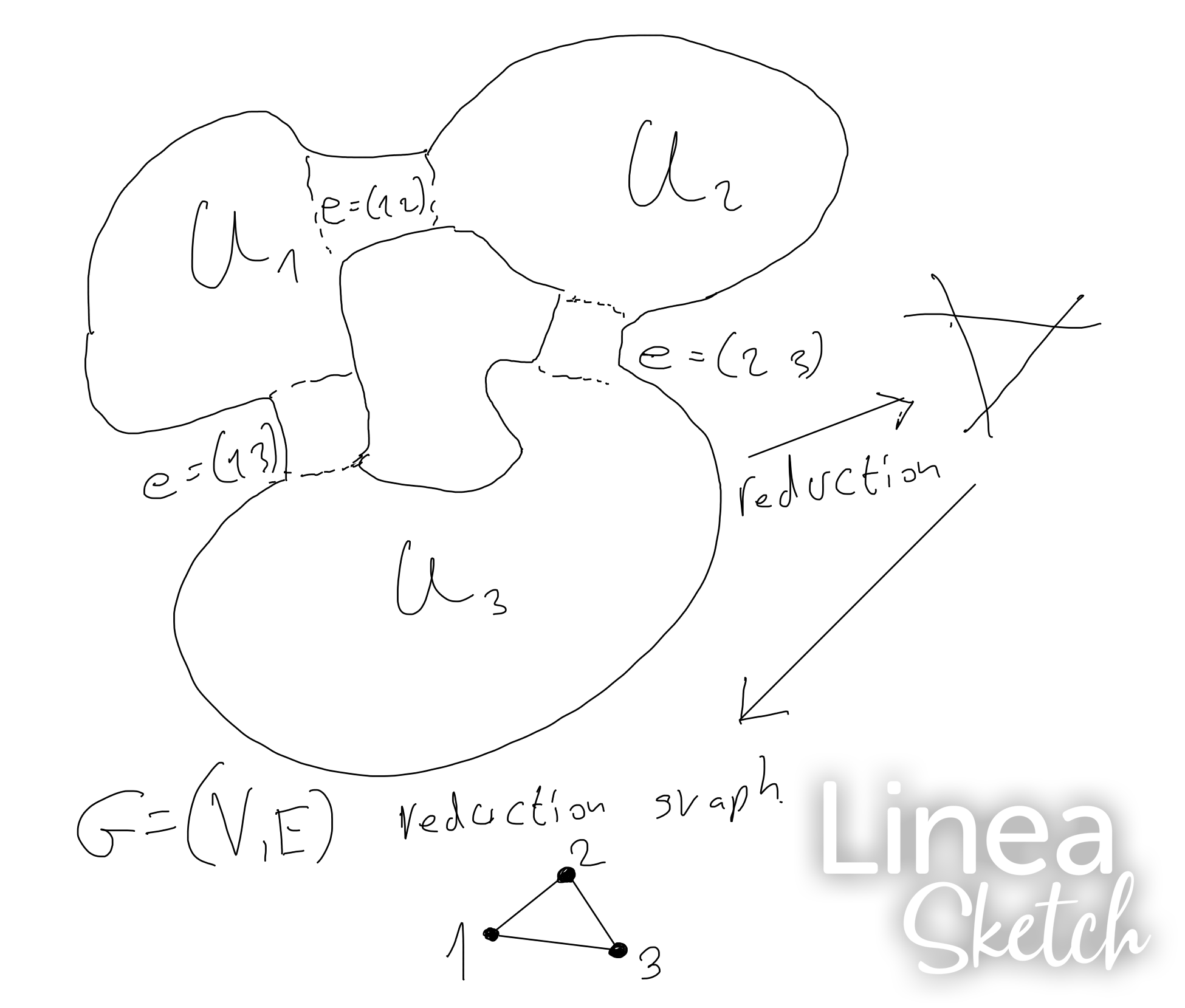
Figure 1. semi-stable curve and its reduction graph.

We give a Crash course on graph cohomology. All of this material is well known. For us, a graph $\Gamma$ has a set $V$ of vertices and $E$ of oriented edges. Each edge $e\in E(\Gamma)$ has a tail and head, $e^{+},e^{-}\in V(\Gamma)$ respectively, and for each edge we have the edge with reverse orientation $-e$ such that $(-e)^{+}=e^{-}$ and $(-e)^{-}=e^{+}$ and $K$ any field, let $K^{V}$ denote as usual the vector space of functions from $V$ to $K$, and $K_{-}^{E}$ the set of functions $E\to K$ which are antisymmetric with respect to orientation-reversing: $f(-e)=-f(e)$. There is a differential $d:K^{V}\to K_{-}^{E}$, $df(e)=f(e^{+})-f(e^{-})$ and we define graph cohomology by

$$H^{1}(\Gamma,K)=K_{-}^{E}/dK^{V}\;.$$

Both $K^{V}$ and $k_{-}^{E}$ have obvious scalar products and the dual operator to $d$ with respect to these, $d^{\ast}:K_{-}^{E}\to K^{V}$, is given by $d^{\ast}g(v)=\sum_{e^{+}=v}g(e)$. The space of harmonic cochains is defined as $\mathcal{H}(\Gamma,K)=\operatorname{Ker}d^{\ast}$.

For a connected $\Gamma$ the harmonic decomposition

(4.4) $$K_{-}^{E}=dK^{V}\oplus\mathcal{H}(\Gamma,K)$$

follows by observing that the kernel of the Laplacian $\Delta=d^{\ast}\circ d:K^{V}\to K^{V}$ is the space of constant functions and its image is its orthogonal complement. We note the following easy observation.

Lemma 4.2.

The projection on $dK^{V}$ coming from the harmonic decomposition (4.4) is simply

$$d\circ\Delta^{-1}\circ d^{\ast}\;.$$

One source of harmonic cochains is the monodromy operator $N$. For a meromorphic form on $X$ with no singularities on the annuli it is defined as

$$N\omega(e):=\operatorname{res}_{e}(\omega)\;,$$

where the residue of an analytic form on an oriented annulus is defined in [24, Lemma 2.1]. The residue theorem for wide open spaces [24, Proposition 4.3] immediately shows that

(4.5) $$d^{\ast}N\omega(v)=\operatorname{res}_{U_{v}}\omega\;,$$

where the right-hand side means the sum of the residues of $\omega$ on $U_{v}$. Recall that a meromorphic form on a curve is said to be of the second kind if all its residues are $0$. For such a form $\omega$ we immediately get from (4.5) that $N\omega$ is harmonic. The monodromy operator as defined here is essentially the same as the one coming from Fontaine’s theory. Indeed, by [22] the space $\mathcal{H}(\Gamma,K)$ embeds into $H_{\textup{dR}}^{1}(X/K)$ and the Fontaine monodromy operator is just the composition of $N$ as defined here with this embedding.

The results of [15] are for a Vologodsky integral with respect to a fixed branch, so at this point we fix such a branch. To state the main result of [15] we point out that as the domains $U_{v}$ are basic wide open spaces with good reduction, forms on them can be Coleman integrated. These integrals extend, once a branch of the logarithm is fixed, to the annuli $e$. This is not part of the general theory and needs to be argued separately (see [6, Section 5]).

Theorem 4.3 ([15]).

Let $\omega$ be a meromorphic form on $X$ and let $F_{\omega}$ be a Vologodsky integral of $\omega$. Then, for each vertex $v$ of $\Gamma(X)$ there exist Coleman integrals $F_{\omega}^{v}$ of $\omega|_{U_{v}}$ such that $F_{\omega}$ equals $F_{\omega}^{v}$ on $U_{v}(K)$. For an oriented edge $e$ let $c_{\omega}(e)=F_{\omega}^{e^{-}}|_{e}-F_{\omega}^{e^{+}}|_{e}\in K$. Then $c_{\omega}$ is a harmonic cochain on $\Gamma(X)$ with values in $K$, $c_{\omega}\in\mathcal{H}(\Gamma(X),K)$.

It is important to observe that $F_{\omega}$ is not a function on the annuli. It is only a function on $K$-rational points and the annuli do not have any such points. This is why the single valued function $F_{\omega}$ can be defined on the $U_{v}$ by Coleman functions that do not match on the intersections. Obviously, one can extend $F_{\omega}$ to the annuli by extending the base field, but this will force a change in the semi-stable model and no contradiction arises (see [15]).

Theorem 4.3 gives a way of recovering Vologodsky integrals on curves, provided one knows how to compute Coleman integrals. Namely, to compute $F_{\omega}$ first choose Coleman integrals $G^{v}$ for $\omega$ on the corresponding $U_{v}$. There is a choice of a constant of integration for each $v$ and one makes such a choice arbitrarily. Then one computes the cochain $c(e)=G^{e^{-}}-G^{e^{+}}$. This cochain has a unique decomposition, by (4.4),

$$c=c_{\omega}+d\gamma\;,\quad c_{\omega}\text{ harmonic, }\gamma\in K^{V}\;,$$

where $\gamma$ is uniquely determined by $d\gamma$ up to an additive constant. The required $F_{\omega}^{v}$ computing a Vologodsky integral of $\omega$ are then clearly given by

$$F_{\omega}^{v}=G^{v}-\gamma(v)\;.$$

Note that by the discussion above we have

$$\gamma=\Delta^{-1}d^{\ast}c\;.$$

To give a flavor of the type of results one might prove using this type of analysis, let us begin by reproving Corollary 2.2 (The reader might find it useful to look first at the very simple case of a Tate elliptic curves considered in Section 3 of [15]). The key to understanding how the description of Vologoksky integration affects the dependency on $\log(p)$ is to analyze what happens at an annulus. Suppose an annulus $e$ is mapped, via a coordinate $z$, to the annulus $|\pi|<|z|<1$ and a form $\omega$ is given, whose local expansion on $e$ is

$$\omega=\sum_{k}a_{k}z^{k}\frac{dz}{z}$$

so that $\operatorname{res}_{e}\omega=a_{0}$ The integral of $\omega$ on the domain which connects to the inner side of $e$ is given by integrating term by term

$$F_{1}=\sum_{k\neq 0}\frac{a_{k}}{k}z^{k}+a_{0}\log(z)+C_{1}$$

for some constant $C_{1}$. To get the integral on the domain connecting to the outer side we first make the change of variables $z=\pi/w$,

$$\omega=-\sum_{k}a_{k}(\frac{\pi}{w})^{k}\frac{dw}{w}\;,$$

giving an integral

$$F_{2}=\sum_{k\neq 0}\frac{a_{k}\pi^{k}}{k}w^{-k}-a_{0}\log(w)+C_{2}\;.$$

Substituting back $z=\pi/w$ we get

$$F_{1}-F_{2}=C_{1}-C_{2}+a_{0}\log(\pi)=C_{1}-C_{2}+\operatorname{res}_{e}\omega\log(\pi)\;.$$

Suppose that $F$ is a Vologoksky integral of $\omega$ with respect to a certain branch $\log(\pi)$. On each $U_{v}$ it is represented by a Coleman integral with a choice of constant of integration, and the chain of differences $c_{\omega}(e)$ is harmonic. It is better to write here $c_{\omega,\log(\pi)}$ to stress the dependency on $\log(\pi)$ According to the above computation, for the same choices of constants of integration, with respect to a different branch of the logarithm $\log^{\prime}(\pi)$, the chain of differences is

(4.6) $$c_{\omega,\log^{\prime}(\pi)}=c_{\omega,\log(\pi)}+(\log^{\prime}(\pi)-\log(\pi))N\omega\;.$$

But since $N\omega$ is harmonic, this chain is harmonic as well, hence the same constants of integration give again the Vologoksky integral. Therefore, the integral is independent of the choice of the branch.

The advantage of this proof is that it applies verbatim for integrals of forms of the second kind, which are therefore also independent of the branch of the logarithm. For general meromorphic forms we have the following easy generalization.

Proposition 4.4.

Let $\omega$ be a meromorphic form on $X$ with no singularites on the annuli. Let $F_{\omega}$ be a Vologodsky integral of $\omega$ with respect to the universal branch. Then, the function $d/d\log(\pi)F_{\omega}$ is constant on each domain $U_{v}$ except near the logarithmic singularities of $\omega$, and associating this constant with the vertex $v$ one gets a function on the dual graph which satisfies

$$\Delta\frac{d}{d\log(\pi)}F_{\omega}(v)=\operatorname{res}_{U_{v}}\omega\;.$$

Proof.

The same analysis as before together with Lemma 4.2 gives that the derivative is

$$-\Delta^{-1}d^{\ast}N\omega$$

and we are done by (4.5). ∎

Note that the above result determines the derivative only up to an additive constant. This is unavoidable since one could in theory have a different constant of integration associated with $F_{\omega}$ for each branch of the logarithm. To avoid this make the integral independent of $\log(\pi)$ at some point, e.g., by setting it to $0$ at that point. However, there are cases where we have the constant built in. For example, if $f$ is a rational function on $X$ and $\omega=d\log(f)$, then it is natural to pick $F_{\omega}=\log(f)$ and this might have a constant of integration which is a multiple of $\log(\pi)$. In fact, we clearly have

$$\frac{d}{d\log(\pi)}\log(f)(v)=\operatorname{ord}_{T_{v}}f\;.$$

Note that this is consistent with [15, Lemma 2.1].

As a particular case, and as a prelude to the discussion in Section 5, let us use Proposition 4.4 to recover local height pairings on curves. In [10] we extended the Coleman-Gross $p$-adic height pairing on curves [21] using Vologodsky integration instead of Coleman integration at primes above $p$, and proved its compatibility with the Nekovář $p$-adic height pairing. When $X$ is a smooth complete curve over a number field $F$, and $D,E$ are two divisors of degree $0$ on $X$, their $p$-adic height pairing $h(D,E)$ is a sum of local terms corresponding to the different finite completions of $F$. if $K$ is such a completion, with respect to a prime above $p$, the local term for $K$ is the trace down to $\mathbb{Q}_{p}$ (we do not discuss this trace here, see Section 5), of the expression

$$(D,E)=\int_{E}\omega_{D}\;.$$

Here, the integral is a Vologodsky integral evaluated at the divisor $E$ while the form $\omega_{D}$ is a specially chosen meromorphic form of the third kind whose residue divisor $\sum_{x}\operatorname{res}_{x}(\omega)\cdot x$ is $D$ (recall that a meromorphic one-form on a curve is of the third kind if it only has simple poles and all of its residues are integers). The determination of a canonical such $\omega_{D}$ is one of the key elements in the construction, but fortunately for us, we do not need to discuss it here, as we will only be interested in

$$\frac{d}{d\log(\pi)}(D,E)=\frac{d}{d\log(\pi)}\int_{E}\omega_{D}\;,$$

and, since $\omega_{D}$ is well-defined up to the addition of a holomorphic form, this quantity is independent of the precise choice by Corollary 2.2.

Proposition 4.5.

The expression

$$\frac{d}{d\log(\pi)}(D,E)$$

equals, up to a fixed multiple, the local height pairing as defined in the proof of  [21, Proposition 1.2].

Proof.

For simplicity, we assume that $D$ and $E$ are formal sum of $K$-rational points and skip the formal argument to show that this is sufficient. The relevant, “rational part”, of the local height pairing is defined in [21] as the intersection product on a regular model $\mathcal{X}$ of $X$, of divisors extending the divisors $D$ and $E$, to divisors which have a zero intersection with each component of the special fiber. In other words, we extend the points in $D$ and $E$ to sections and then add rational multiples of the components of the special fiber to satisfy the requirement. Clearly, it suffices to do this for only one of the divisors. So let $D$ and $E$ denote also the divisor on $\mathcal{X}$ obtained by extending the points in $D$ and $E$ to sections over $\mathcal{O}_{K}$ and let $\tilde{D}=D+\sum_{v}a_{v}T_{v}$ be the required extension, so that we need to compute

(4.7) $$\tilde{D}\cdot E=D\cdot E+\sum_{v}a_{v}D\cdot T_{v}\;.$$

Using Lemma 4.1 it is easy to see that we only need to account for the second term on the right-hand side of (4.7) Clearly, $\operatorname{res}_{U_{v}}\omega_{D}=\deg_{U_{v}}D$, where the right-hand side indicates the degree of the part of $D$ inside $U_{v}$. If $f=\Delta^{-1}(v\mapsto\deg_{U_{v}}D)$ then we easily see that the “global” contribution to the derivative is

$$\sum_{v\in V}\deg_{U_{v}}Ef(v)=E\cdot\sum f(v)T_{v}$$

and we are left with showing that $f(v)=a_{v}+\textup{const}$. The condition on $\tilde{D}$ is that for every $w\in V$ we have

$$0=(D+\sum_{v}a_{v}T_{v})\cdot T_{w}=\deg_{U_{w}}D+\sum_{v}a_{v}T_{v}\cdot T_{w}\;.$$

The sum on the right is clearly only over $v$ for which there exist an edge $(v,w)$, and over $v=w$. Our assumptions about the reduction imply that for $v\neq w$ in the sum we have $T_{v}\cdot T_{w}=1$. Furthermore, since the special fiber is just $\sum_{v}T_{v}$ and its intersection with each $T_{w}$ is $0$, we see that

$$T_{w}\cdot T_{w}=-\sum_{(v,w)\in E}1$$

so that we have

$$0=\deg_{U_{w}}D+\sum_{(v,w)\in E}a_{v}-a_{w}\;.$$

This gives on $v\to a_{v}$ the same condition as the condition on $f$, making them equal up to a constant as required. ∎

Remark 4.6.

As mentioned in the introduction, a similar observation has been made by Colmez [25], in the proof of Théorème II.2.18. The method is quite different. Colmez simply notes that the derivative satisfies the basic list of properties which uniquely characterize the height pairing. Here on the other hand, we directly show that the result is the same as the construction of the local height pairing in terms of intersection theory.

In order to treat iterated integrals we need the work of Katz and Litt [32]. We will present it in an equivalent way (the equivalence with the original formulation was proved by Katz in a private communication). The new formulation is a direct generalization of [15].

To describe the result, choose for simplicity a $K$ rational point $x_{v}$ in each domain $U_{v}$. Let $(M,\nabla)$ be a unipotent connection on $X$. We have “monodromy matrices” corresponding to the following “loops” associated with each edge $e=(v,w)$: Start with $x_{v}$, use Vologodsky parallel transport to go to $x_{w}$, use Coleman parallel transport to go to the side of the annulus $e$ on the $U_{w}$ side, cross to the $U_{v}$ side of $e$ and finally Coleman parallel transport back to $x_{v}$ (see Figure 2).

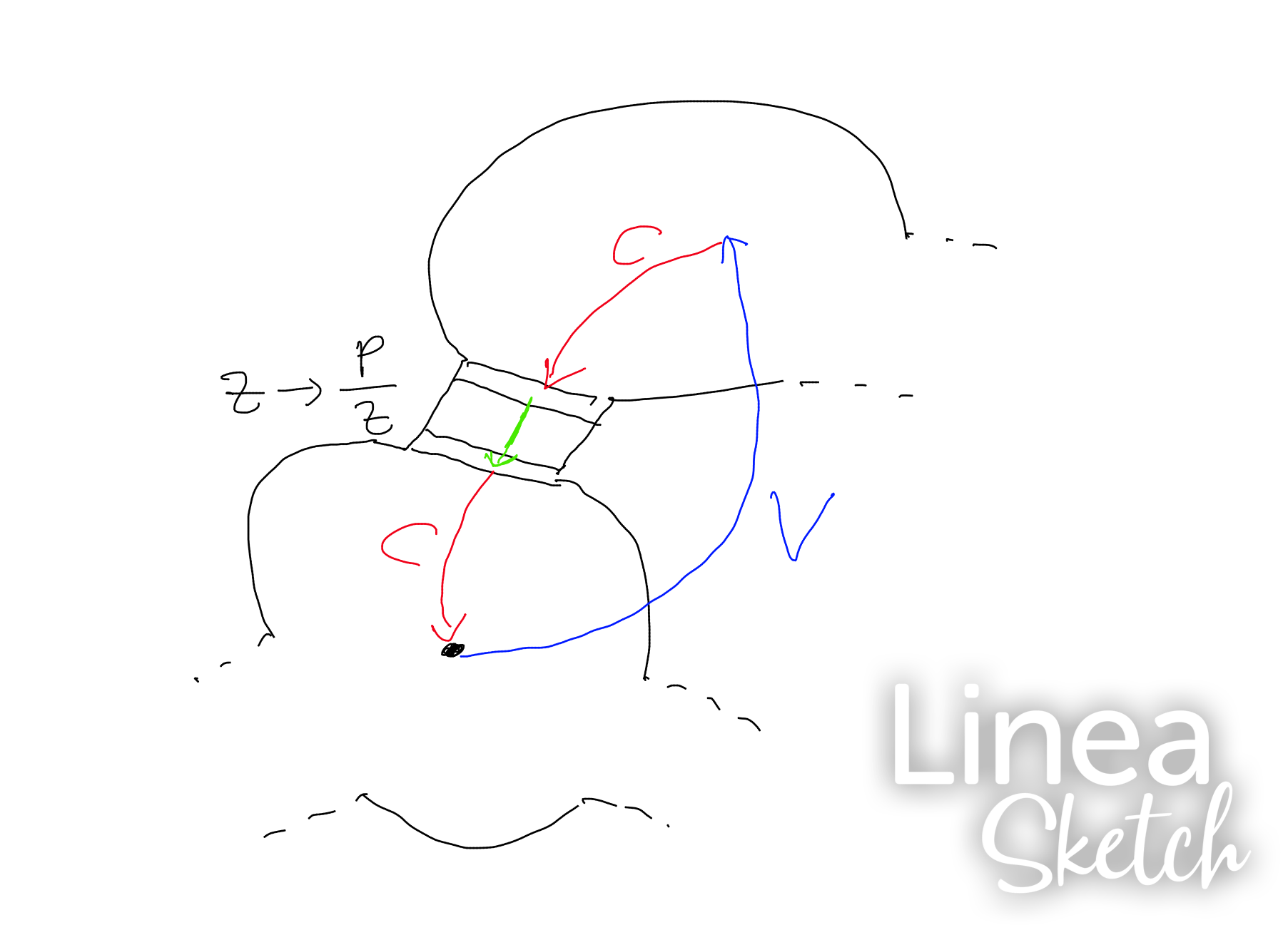
Figure 2. The loop determining $A(e)$.

This gives an operator on the fiber at $x_{v}$ of $M$. Up to conjugacy it is independent of the choice of $x_{v}$. Denote it by $A(e)$.

Theorem 4.7 (Reinterpreted Katz-Litt).

The association $e\to A(e)$ is harmonic in the sense that for each $v\in V$, $\sum_{e^{+}=v}\log(A(e))=0$.

In [13] we use this result to derive a formula for the derivative with respect to $\log\pi$ of certain iterated Vologodsky integrals.

Theorem 4.8 ([13]).

Suppose $\omega$ and $\eta$ are two forms of the second kind on $X$. Let

$$F=\int(\omega\int\eta)$$

with respect to the universal branch. The funcion

$$\frac{d}{d\log(\pi)}F$$

is constant on each domain $U_{v}$ except near the singularities of $\omega$ or $\eta$, and associating this constant with the vertex $v$ one gets a function on the dual graph which satisfies

$$\Delta\frac{d}{d\log(\pi)}F_{\omega}(v)=\frac{1}{2}\sum_{e^{+}=v}c_{\eta}(e)\operatorname{res}_{e}\omega-c_{\omega}(e)\operatorname{res}_{e}\eta-\sum_{e^{+}=v}\langle\int\eta,\int\omega\rangle_{e}\;.$$

Here, $c_{\omega}$ and $c_{\eta}$ are the harmonic cochains associated with $\omega$ and $\eta$ in Theorem 4.3 (with respect to the canonical branch) and the last term is the local index on an annulus (see [5]).

5. $p$-adic heights

In this section we report on work with Müller and Srinivasan [12]. In this work we describe a $p$-adic analogue to the theory of heights associated to line bundles with adelic metrics [51]. Our main interest is in applications to the problem of finding rational point on curves through the method known as “Quadratic Chabauty” [3, 1, 2], but the theory of heights we develop is of independent interest. For analogy, let us first quickly review the classical theory.

Let $F$ be a number field with a system of absolute values $|~|_{\nu}$ satisfying the product formula. Let $X$ be a smooth complete variety over $F$.

Definition 5.1.

An adelic line bundle on $X$ is a line bundle $\mathcal{L}$ over $X$ together with a collection of norms, $\|~\|_{\nu}$ on the line bundle $\mathcal{L}\otimes F_{\nu}$, for each place, finite or infinite, $\nu$ of $F$. This collection needs to satisfy certain conditions, which guarantee, among other things, that the associated height

$$h_{\hat{L}}:X(F)\to\mathbb{R},\quad h_{\hat{L}}(x)=\sum_{\nu}\log\|w\|_{\nu}$$

is a finite sum, where $w$ is any vector in the fiber of $L$ over $x$.

From the product formula it is immediate to see that the height indeed depends only on $x$ and not on the particular choice of $w$. We avoid discussing conditions on the norms for ease of presentation, since we will mostly be concerned with the $p$-adic theory, and since canonical norms that we want to study satisfy these automatically.

Following Tate’s definition of canonical heights for Abelian varieties, one can attempt to obtain canonical heights in various situations. The following scenario, which we dub “the dynamical situation”, is considered by Zhang [51](see also [17]). Suppose that $f\colon X\to X$ is an endomorphism $X$ and the line bundle $\mathcal{L}$ is such that there exists an integer $d>1$ and an isomorphism

(5.1) $$\beta\colon\mathcal{L}^{\otimes d}\to f^{\ast}\mathcal{L}\;.$$

Zhang constructs, at each place $\nu$, a canonical norm on $\mathcal{L}_{v}$ for which $\beta$ is an isometry (we will say that the metric is compatible with the dynamical situation), by starting with any norm $\|\cdot\|_{\nu}$ and repeatedly replacing $\|\cdot\|_{\nu}$ with $(\beta^{-1}f^{\ast}\|\cdot\|_{\nu})^{\frac{1}{d}}$ and taking a limit. The resulting local metrics turn out to give an adelic metric. In the case where $X$ is an abelian variety, $f:X\to X$ is the multiplication by $2$ map and $\mathcal{L}$ is a symmetric line bundle on $X$, one gets the Tate canonical height associated with $\mathcal{L}$.

The $p$-adic analogue of the above picture is considered in [12]. The $p$-adic analogue of the system of absolute values satisfying the product formula is a continuous idèle class character

$$\chi=\sum_{\nu}\chi_{\nu}\colon\mathbb{A}_{F}^{\times}/F^{\times}\to{\mathbb{Q}}_{p}\;.$$

The local components $\chi_{\nu}$ are the analogues of the logs of the absolute values and the fact that the character vanishes on $F^{\times}$ is the analogue of the product formula. Note the important difference from the classical case: The primes above $\infty$ play no role.

For $\nu\mid p$, there is a decomposition

(5.2)

for some ${\mathbb{Q}}_{p}$-linear trace map $t_{\nu}$ and some choice of a branch $\log_{\nu}$ of the $p$-adic logarithm. In analogy with the classical case we can define local norms, or rather, logs of local norms, on a line bundle $L$, to be functions $\ell_{\nu}$ on the total space of $L$ minus the zero section, which satisfy the relation

$$\ell_{\nu}(\alpha w)=\chi_{\nu}(\alpha)+\ell_{\nu}(w)\;.$$

However, at all places $\nu$ not above $p$ one has the property $\chi_{\nu}(\alpha)=\nu(\alpha)\chi(\pi_{\nu})$, where $\pi_{\nu}$ is a uniformizer at $\nu$ and we write $\nu$ also for the associated valuation, so that it makes sense to divide the function by $\chi_{\nu}(\pi_{\nu})$. With this in mind we make the following.

Definition 5.2.

Let $K$ be a finite extension of $\mathbb{Q}_{q}$, for some finite prime $q$. Let $X$ be a variety over $K$ and let $\mathcal{L}$ be a line bundle over $X$. Then, a $p$-adic metric on $\mathcal{L}$ is:

• For $q=p$ a log function

  $$\log:\mathcal{L}^{\times}:\mathcal{L}-0\to\overline{K}$$

  A function satisfying $\log(\alpha w)=\log_{\nu}(\alpha)+\log(w)$, $\alpha\in K^{\times}$, $w\in\mathcal{L}_{x}$, where $\log_{\nu}$ is the branch of the $p$-adic logarithm determined by (5.2).

• For $q\neq p$ a valuation

  $$\operatorname{val}:\mathcal{L}^{\times}\to{\mathbb{Q}}$$

  satisfying $\operatorname{val}(\alpha w)=\nu(\alpha)+\operatorname{val}(w)$ where $\nu$ is the valuation on $K^{\times}$, normalized so that $\nu(\pi_{\nu})=1$.

Let $F$ be a number field, $X$ a variety over $F$ and $\mathcal{L}$ a line bundle over $X$. An adelic metric on $\mathcal{L}$ is a collection of metrics for the completions of $\mathcal{L}$ over all finite places of $F$, satisfying a certain technical condition (that the valuation is almost always a “model valuation”). A line bundle $\mathcal{L}$ over $X$ together with an adelic metric will be called an adelically metrized line bundle, usually denoted $\hat{\mathcal{L}}$. The $p$-adic height $h_{\hat{\mathcal{L}}}:X(F)\to{\mathbb{Q}}_{p}$ associated to the adelically metrized line bundle $\hat{\mathcal{L}}$ is given by the formula

$$h_{\hat{L}}(x)=\sum_{\nu|p}t_{\nu}\log_{\nu}(w)+\sum_{\nu\nmid p}\operatorname{val}_{\nu}(w)\cdot\chi_{\nu}(\pi_{\nu})$$

where $w$ is any vector in the fiber of $\mathcal{L}$ over $x$.

As in the classical case, it is obvious that the definition of the height is independent of the choice of $w$.

Remark 5.3.

One can define valuations that take values in other groups. This will be useful later on (see Proposition 5.6). For the global theory and the construction of heights, only $\mathbb{Q}$-valued valuations are useful.

The part of the theory which involves finite primes different from $p$, is in many respects joint between the $p$-adic and the classical case. Indeed, given a valuation $\operatorname{val}_{\nu}$, where $\nu$ is a place above a finite prime $q\neq p$, such that the associated absolute value is $|~|_{\nu}=c^{\nu(~)}$ for some $c\in(0,1)$, the function

$$\|~\|_{\nu}=c^{\operatorname{val}_{\nu}(~)}$$

is a norm in the classical sense. Clearly, it is not the most general type of norm. However, it turns out that in many situations the norms one considered are in fact of this form. Conversely, if we obtain a norm taking values in $c^{{\mathbb{Q}}}$, then taking the log with respect to $c$ gives us a valuation.

Let us turn now to the situation above $p$. As we mentioned for the classical theory, defining heights using metrics can be done without any serious restrictions on the type of metric used. However, in practice one imposes some restrictions on the norms. In the $p$-adic situation, this is both a restriction and a good way of constructing metrics. Recall that if $K$ is a finite extension of $\mathbb{Q}_{p}$, and $\mathcal{L}/X$ is a line bundle over a smooth variety over $K$, then a $p$-adic metric on $\mathcal{L}$ consists of a log function on the total space of $\mathcal{L}$ minus the zero section. It is natural to ask that this log function is a Vologodsky function. We in fact ask for a far stronger condition: that log is at most a second iterated Vologodsky integral. Let us call such log functions admissible (note, in [7] we called these log functions and what we now call log functions we called there Pseudo log functions). The key result concerning these functions, allows their characterization as well as construction using the notion of curvature. This is described in the following Theorem.

Theorem 5.4 ([7, Proposition 4.4]).

Suppose $X$ is proper and let

$$\cup:H_{\textup{dR}}^{1}(X/K)\otimes\Omega^{1}(X)\to H_{\textup{dR}}^{1}(X/K)$$

be the cup product map. Suppose $ch_{1}(\mathcal{L})$ is in the image of $\cup$. Then one can associate to each admissible log function on $\mathcal{L}$ a curvature form, $\alpha\in H_{\textup{dR}}^{1}(X/K)\otimes\Omega^{1}(X)$, such that $\cup(\alpha)=ch_{1}(\mathcal{L})$ Conversely, any curvature form $\alpha$ cupping to $ch_{1}(\mathcal{L})$ is the curvature of an admissible log function on $\mathcal{L}$, unique up to an integral of $\omega\in\Omega^{1}(X)$.

We will not explain the construction of the curvature or the proof of the theorem. An explicit description of a log function with a given curvature is not so easy in general. However, for the case of curves, a fairly easy description can be given as follows.

Theorem 5.5 ([12, Section 3]).

Let $\mathcal{L}$ be a line bundle over a complete curve $X$ over $K$ and let $\alpha$ be a curvature form cupping to $ch_{1}(\mathcal{L})$. Fix a rational section $s$ of $\mathcal{L}$. To determine a log function on $\mathcal{L}$ it suffices to determine $\log(s)$. Let $\alpha=\sum_{i}\omega_{i}\otimes[\eta_{i}]\in\Omega^{1}(X)\otimes H_{\textup{dR}}^{1}(X)$ for some holomorphic forms $\omega_{i}\in\Omega^{1}(C)$ and forms of the second kind $\eta_{i}$ with corresponding cohomology classes $[\eta_{i}]\in H_{\textup{dR}}^{1}(C)$. Then, the formula

(5.3) $$d\log_{\mathcal{L}}(s)=\sum\omega_{i}\int\eta_{i}+\gamma,$$

determines a log function on $\mathcal{L}$ with curvature $\alpha$. Here, $\gamma$ is any meromorphic form with the property that the right-hand side has only simple poles on $X$ and its residue divisor is exactly $\operatorname{div}(s)$

We observe that the degree of freedom in choosing $\gamma$ is exactly adding a holomorphic form, so the degree of freedom in the log function is exactly adding the integral of a holomorphic form, which is exactly the degree of freedom in Theorem 5.4.

If we try to copy the construction of canonical norms in Dynamical situations to the $p$-adic setting, we immediately observe a problem: The limiting procedure defining the norms will not converge $p$-adically. Thus, another idea is required for finding canonical metrics.

For $q\neq p$, one can hope that a canonical norm obtained through the limiting procedure over $\mathbb{R}$ actually takes values in some $c^{\mathbb{Q}}$, hence a valuation may be obtained from it. This will not work for $q=p$, where the log function is truly $p$-adic.

Instead of using limiting methods, one may use the theory of the curvature, Theorem 5.4. Consider then $K$ a finite extension of $\mathbb{Q}_{p}$, a complete smooth variety $X$ over $K$, a line bundle $\mathcal{L}$ over $X$, an endomorphism $f:X\to X$ and an isomorphism (5.1). If the log function $\log_{\mathcal{L}}$ with curvature $\alpha$ makes $\beta$ an isometry, then we have

(5.4) $$f^{\ast}\alpha=d\alpha$$

This is consistent with the fact that $f^{\ast}ch_{1}(\mathcal{L})=dch_{1}(\mathcal{L})$, which needs to hold since $\alpha$ cups to $ch_{1}(\mathcal{L})$. Conversely, suppose that (5.4) holds with $\alpha$ a curvature form cupping to $ch_{1}(\mathcal{L})$. Then, for any log function on $\mathcal{L}$ with curvature $\alpha$, which exists by Theorem 5.4, The two log functions, $d\log_{\mathcal{L}}$ and $\beta^{-1}f^{\ast}\log_{\mathcal{L}}$, on $\mathcal{L}^{\otimes d}$, have the same curvature and therefore, again by Theorem 5.4, defer by the integral of a holomorphic form on $X$. At this point one can study how this form is changed when $\log_{\mathcal{L}}$ is changed by the integral of a holomorphic form, and, depending on the action of $f^{\ast}$ on $\Omega^{1}(X)$, it’s often possible to make $\beta$ an isometry as required.

One case of the above was key to [12]. There we construct canonical metrics on a symmetric line bundle $\mathcal{L}$ on an abelian variety $X$. In this case $f$ is the multiplication by $2$ map and $d=4$. For further details see [12, 4.2.1].

At this point we apply the general theme of this work. Up to now we defined the $p$-adic metric above $p$ with a fixed choice of a branch, dictated by the idèle class character $\chi$. Now, instead, we will consider the metric as a Vologodsky function with respect to the universal branch of the logarithm, and differentiate with respect to $\log(p)$. As we will see, this gives valuations, in the more general sense of Remark 5.3, i.e., with values in more general groups than the additive group of the rationals.

Proposition 5.6.

Let $\log_{\mathcal{L}}$ be a log function with the universal branch of the logarithm. Then $d/d\log(\pi)\log_{\mathcal{L}}$ is a $\overline{K}$-valued valuation on $\mathcal{L}$. We call it the Vologodsky valuation associated with the log function.

Proof.

This is immediate from (1.4). ∎

Proposition 5.7.

The Vologodsky valuation associated with a log function on $\mathcal{L}$ depends only on the associated curvature $\alpha$. Thus, we may denote it $\operatorname{val}_{\alpha}$. This valuation is defined for every curvature form $\alpha$ cupping to $ch_{1}(\mathcal{L})$.

Proof.

This is clear from Corollary 2.2. ∎

The following is obvious.

Proposition 5.8.

Let $\mathcal{L}$ be a line bundle on $X$ and let $\alpha$ be a curvature form cupping to $ch_{1}(\mathcal{L})$. If $g:Y\to X$ is a morphism, then $g^{\ast}\operatorname{val}_{\alpha}=\operatorname{val}_{g^{\ast}\alpha}$

Corollary 5.9.

In the dynamical situation, suppose $\alpha$ is a curvature form cupping to $ch_{1}(\mathcal{L})$ and satisfying $f^{\ast}\alpha=d\alpha$. Then, $\beta$ is an isometry (up to a constant) for the valuation $\operatorname{val}_{\alpha}$.

Proof.

The two valuations one obtains on $\mathcal{L}^{\otimes d}$ have the same curvature. ∎

Thus, in dynamical situation, there are (at least) two ways to construct a compatible valuation locally at a place above the prime $q$. One method is via limiting procedures using norms over $\mathbb{R}$, hoping that the resulting norm has values in some $c^{\mathbb{Q}}$. The other is via $q$-adic analysis and curvature forms. The former method has several advantages

• It does not need to assume the existence of a well-behaved curvature form

• The latter method may not produce $\mathbb{Q}$-valued valuations. The former method may produce norms which are not coming from valuations, but these may still be used in the theory of heights while non- $\mathbb{Q}$-valued valuations are useless there.

We note though that for any line bundle $\mathcal{L}$ on an abelian variety $X$ the Vologodsky valuation associated with any curvature form for $\mathcal{L}$ is $\mathbb{Q}$-valued. In fact, it does not depend on the curvature but only on the line bundle itself and is the canonical valuation so may be used for the computation of the canonical height. This is proved in [12, Theorem 9.24].

The method of Vologodsky valuations has one very important advantage. If a valuation is constructed in a dynamical situation for the line bundle $\mathcal{L}$ over $X$ using the limiting procedure, then there would be some way to control, compute or approximate it over $X$. However, if we pull back via $g:Y\to X$, there will be no obvious way to compute the pulled back valuation over $Y$. On the other hand, using Vologodsky valuations, the pulled back valuation is associated with the pulled back curvature, and is therefore, at least in principle, computable. This is especially true if $Y$ is a curve, as Theorem 5.5 provides an explicit description of the log function in terms of the curvature, and Theorem 4.8 provides a way of computing the associated valuation. In [13] we use this to explicitly compute the pullback to a curve of the canonical valuation on a symmetric line bundle on the Jacobian of the curve, with applications to Quadratic Chabauty.

6. The unipotent Albanese map

The classical Albanese map between a variety and its Albanese variety has a non-abelian analogue, the Unipotent Albanese map first appearing in its Hodge incarnation in the work of Hain [29] and later becoming a cornerstone of Kim’s non-abelian Chabauty’s method [33, 34].

Our Goal is to discuss the case of curves with semi-stable reduction, but doing so in a rather informal manner. In particular, we do not claim any relation with the étale theory.

Let us discuss things first is some generality. Suppose $X$ is a variety over a field $K$, which for the moment can be any field. We assume that we can define for $x_{0}\in X(K)$ some sort of fundamental group $G=\pi_{1}(X,x_{0})$, possibly with some extra structure, and, given another rational point $x\in X(K)$, a fundamental path space $\pi_{1}(X,x_{0},x)$, again with some extra structure, which is a right torsor for $G$ with compatible structures (using the theory of Tannakian categories one can often streamline the meaning of these compatible structures).

Definition 6.1.

Let $\operatorname{Alb}(G)$ be the set of isomorphism classes of $G$-torsors with compatible structure and define the abstract Albanese map as the map

$$\alpha_{X}:X(K)\to\operatorname{Alb}(\pi_{1}(X,x_{0}))$$

sending $x\in X(K)$ to the isomorphism class of the torsor $\pi_{1}(X,x_{0},x)$.

Perhaps the most obvious example of an abstract Albanese map is the one for which $\pi_{1}$ is the étale fundamental group (respectively étale path space) of $\overline{X}:=X\otimes_{K}\overline{K}$, which is a group (respectively a torsor) with an action of $\operatorname{Gal}(\overline{K}/K)$. In this case we clearly have

$$\operatorname{Alb}(\pi_{1}(X,x_{0}))=H^{1}(\operatorname{Gal}(\overline{K}/K),\pi_{1}(\overline{X},x_{0}))\;,$$

the non-abelian cohomology of $\operatorname{Gal}(\overline{K}/K)$ with coefficients in $\pi_{1}(\overline{X},x_{0})$.

In the second example $K$ is a finite extenion of $\mathbb{Q}_{p}$, $X$ is a proper variety over $K$ with good reduction and the fundamental group is the unipotent de Rham one, the pro-algebraic group associated by Tannakian duality to the category of unipotent integrable connections on $X$ with the fiber functor of taking the fiber at $x_{0}$. This has a filtration and an action of a Frobenius automorphism (we take the linear Frobenius and not the semi-linear one for convenience), and path spaces have the same structure. In [8] we proved the following result.

Theorem 6.2.

We have a canonical isomorphism

(6.1) $$\operatorname{Alb}(\pi_{1}^{dR}(X,x_{0}))\cong F^{0}\backslash\pi_{1}^{dR}(X,x_{0})(K)$$

Furthermore, there exists a correspondence between regular functions on $\pi_{1}^{dR}(X,x_{0})$, left invariant under $F^{0}$, and Coleman functions on $X$ such that if the function $f$ corresponds to the Coleman function $F$ on $X$, then

$$f(\alpha_{x}(x))=F(x),\quad x\in X(K)\;.$$

For the proof we need to recall that function on an affine group scheme $G$ over a field $K$ can be given by “matrix coefficients”. These are defined by triple $(V,v,s)$, where $V$ is a finite dimensional representation of $G$, $v\in V$ and $s\in V^{\ast}$. Such a triple defines a function on $G$ by the formula

$$(V,v,s)(g)=s(gv)\;.$$

There are obvious relations between such triple that produce the same function. In particular, if $T:V\to V^{\prime}$ is a $G$-map, then the triple $(V,v,T^{\ast}s^{\prime})$ and $(V^{\prime},Tv,s^{\prime})$ produce the same function. If $G$ is the fundamental group of a neutral Tannakian category $\mathbb{T}$, with fiber functor $\omega$, then these triple are given in terms of $\mathbb{T},\omega$ as $(V,v,s)$ where $V\in\mathbb{T}$, $v\in\omega(V)$ and $s\in\omega(V)^{\ast}$. This allows a direct construction of the underlying Hopf algebra. In the standard definition one uses in the construction $\omega(V)\otimes\omega(V)^{\ast}$ but it is easy to see that simple tensors suffice.

Lemma 6.3.

Let $\delta:H\to G$ be a homomorphism of affine group schemes over $K$. A function $f:G\to K$ is $\delta(H)$ left invariant if and only if it can be represented by a triple $(V,v,s)$ where $s$ is an $H$-homomorphism $V\to K$, with $K$ having the trivial $H$-action.

Proof.

Clearly if such a representation exists, the function is left invariant. Conversely, suppose $f$ is $H$ invariant from the left and is represented by a triple $(V,v,s)$. By replacing $V$ with a sub $G$-module we may assume that $v$ generates $V$ as a $G$-module. But then the equation $s(\delta(h)gv)=s(gv)$ for every $g\in G$ and $h\in H$ implies that $s(\delta(h)w)=s(w)$ for every $w\in V$. ∎

Proof of Theorem 6.2.

By [6, Corollary 3.2] each torsor $P$ for $G=\pi_{1}^{dR}(X,x_{0})$ has a canonical Frobenius invariant element $\gamma_{\phi}$ (In Section 2 we called it $\gamma_{x,y}$, a path connecting the two points, but the proof of the theorem, which is an immediate consequence of [6, Theorem 3.1] clearly applies to any path space for $G$). Pick any $\gamma_{dR}\in F^{0}P$. Then $\gamma_{\phi}=\gamma_{dR}g$ for a unique $g\in G$. Any other such choices of $\gamma_{dR}$ will be of the form $\gamma_{dR}h$ for some $h\in F^{0}G$, replacing $g$ by $hg$. This establishes the bijection (6.1). Suppose now that $f:G\to K$ is a regular function that is invariant from the left under $F^{0}$. By [28, Remark 3.8] the subgroup $F^{0}G$ is the image of $H$, the fundamental group of the neutral Tannakian category of unipotent vector bundles, under the map induced by the functor that forgets the connection on bundles with connections. Let $((M,\nabla),v,s)$ be a representation for $f$ whose existence is guaranteed by Lemma 6.3, so $s$ is an $H$-homomorphism. This immediately translates to it being the fiber at $x_{0}$ of a map of vector bundles, which we continue to call $s$. With the new interpretation of $s$, the triple $((M,\nabla),v,s)$ is now a Coleman function $F$. Its value at $x$ is by definition

$$F(x)=s(\gamma_{\phi}v)\;.$$

The value of $f$ on $\alpha(x)=g$ is $s(gx)$. The result now follows because

$$s(\gamma_{\phi}v)=s(\gamma_{dR}(gv))=\gamma_{dR}(s(gv)=s(gv)\;.$$

The last two equalities follow because $\gamma_{dR}$, being in $F^{0}$, commutes with arbitrary morphisms of vector bundles, in particular $s$, and on the trivial line bundle it is just the identity. ∎

Next we consider a variety $X$ with semi-stable reduction over $K$. We then should have a similar picture with a fundamental group $G=\pi_{1}(X,x_{0})$ in the category of filtered $(\varphi,N)$-modules, and a corresponding Albanese map. To be more precise, There is a triple $G=(G_{cr},G_{dR},I_{\pi})$ consisting of an affine group scheme $G_{cr}$ over $K_{0}$ with Frobenius and monodromy operators, an affine group scheme $G_{dR}$ with a filtration, and a comparison isomorphism

$$I_{\textup{HK},\pi}:G_{cr}\otimes_{K_{0}}K\to G_{dR}$$

depending on the choice of a uniformizer $\pi$. The dependency on $\pi$ is such that if we change to $\pi^{\prime}$ we have, exactly as in (3.6),

(6.2) $$I_{\pi^{\prime}}=I_{\pi}\circ\exp(\log(\pi^{\prime}/\pi)N)\;.$$

Note that $N$ (and any multiple of it), being a topologically nilpotent derivation of a Hopf algebra, can be exponentiated to an automorphism of the algebra, hence of the associated affine group scheme.

Remark 6.4.

We intentionally wrote should have. There have been many approaches to the unipotent fundamental group in the log scheme or semi-stable case (a probably not inclusive list includes [35, 36, 32, 49, 26, 46] ). Not all of them state all required results. For example, to the best of our knowledge, the dependency on the uniformizer of the Hyodo-Kato isomorphism is only hinted to in the introduction to [36]. Also, while it is often claimed that all of these approaches are the same, this seems to never be actually proved, excluding some results in [18]. In particular, to actually make all of this into actual theorems, the theory should be compared with the theory of Vologodsky.

The Albanese set $\operatorname{Alb}(G)$ is the set of isomorphism classes of $G$ torsors with compatible structures $P=(P_{cr},P_{dR},I_{\pi})$ in the obvious sense.

Proposition 6.5.

There exists a bijection

$$P\mapsto(P_{c,\pi},P_{d}):\operatorname{Alb}(G)\to(F^{0}\backslash G_{dR})\times\operatorname{Nil}(G_{cr})$$

where $\operatorname{Nil}(G_{cr})$ classifies compatible $N$ on the trivial torsor $G_{cr}$ with its Frobenius.

Proof.

Let $P$ be a $G$ torsor. By [49] the torsor $P_{cr}$ has a canonical path $\gamma_{\phi}$. This path is fixed by Frobenius. As a torsor with a Frobenius action, $P_{cr}$ is therefore trivial and $P_{dR}$ is trivialized by $I_{\pi}(\gamma_{\phi})$. The set $\operatorname{Alb}(G)$ is thus the product of the possible Filtrations on $G_{dR}$ as a $G_{dR}$-torsor, with $\operatorname{Nil}(G_{cr})$. The former is clearly classified by $F^{0}\backslash G_{dR}$. ∎

Note that since the Vologodsky path is not killed by monodromy, there is still some wiggling room for the monodromy, and $\operatorname{Nil}(G_{cr})$ is not trivial. Also note that the map to $F^{0}\backslash G_{dR}$ depends on the choice of the uniformizer $\pi$, since the Vologodsky path needs to be imported via $I_{\pi}$ to $G_{dR}$ in order to define it.

The map in Proposition 6.5 is explicitly given as follows

(6.3) $$P_{c,\pi}=\gamma_{dR}^{-1}I_{\pi}(\gamma_{\phi})\;,\quad P_{d}=\gamma_{\phi}^{-1}N(\gamma_{\phi})\;.$$

The element $N(\gamma_{\phi})$ belongs to $\operatorname{Lie}(G_{cr})$ and characterises $P_{d}$. Vologodsky theory puts some restrictions on this element, which we will not attempt to describe here.

Remark 6.6.

The product decomposition of the Albanese was already observed by Betts.

Definition 6.7.

The compositions of the Albanese map $X(K)\to\operatorname{Alb}(G)$ with the projections on the factors $F^{0}\backslash G_{dR}$ and $\operatorname{Nil}(G_{cr})$ will be called the continuous and discrete components of the semi-stable Albanese map respectively, denoted $\alpha_{c,\pi}$ and $\alpha_{d}$ respectively.

Theorem 6.8.

For each choice of uniformizer $\pi$, the continuous component of the semi-stable Albanese map is computed using Vologodsky integrals: There exists a correspondence between regular functions on $G_{dR}$, left invariant under $F^{0}$, and Vologodsky functions with respect to the branch of the logarithm determined by $\log(\pi)=0$, such that if the regular function $f:G_{dR}\to K$ corresponds to the Vologodsky function $F$ on $X$, then

$$f(\alpha_{c,\pi}(x))=F(x),\quad x\in X(K)\;.$$

The discrete component of the semi-stable Albanese is the logarithmic derivative, with respect to $\log(\pi)$ of the continuous component:

$$P_{c,\pi}^{-1}\frac{d}{d\log(\pi)}P_{c,\pi}=I_{\pi}(P_{d})\;.$$

Proof.

The statement about the continuous component is word for word the proof in the good reduction case. The second statement is obtained by deriving (6.3) with respect to $\log(\pi)$ using (6.2). result ∎

There similarity between the construction in this section and the discussion of syntomic regulators in Section 3, and in particuar Theorem 3.8, should be obvious. We have no attempted though to spell out what this result means in specific situations.

7. Toric regulators

In this section we recall the main results of our paper [14] with Wayne Raskind and relate it to the main theme of this paper.

In [14] we defined (conditionally since some reasonable conjectures are assumed) a new type of regulator maps. It applied to varieties $X$ over a $p$-adic field $K$ with so called “totally degenerate” reduction. This means that $X$ is smooth projective, has strictly semi-stable reduction, and the components of its reduction have all of their cohomologies generated by cycles (see [45, Section 2] for a precise definition). The target of the toric regulator is a “toric intermediated Jacobian” which is a $p$-adic torus $\operatorname{CoKer}:T^{0}\to T^{-1}\otimes K^{\times}$, where $T^{\ast}$ are finitely generated ${\mathbb{Z}}$-modules whose definition we recall shortly. Note that $T^{0}$ and $T^{-1}$ may not be of the same rank.

Some simple examples of toric regulators include:

• The identity map $H_{\mathcal{M}}^{1}(K,1)=K^{\times}\to K^{\times}$

• For $E/K$ a Tate elliptic curve $\mathbb{G}_{m}/q^{{\mathbb{Z}}}$ the identity map

  $$H_{\mathcal{M}}^{2}(E,1)_{0}\cong E(K)\to K^{\times}/q^{{\mathbb{Z}}}$$

• More generally, for a Mumford curve $X$ with Jacobian $J$, the Abel map $X(K)\to J(K)$, where $J(K)$ is viewed as a $p$-adic torus via its $p$-adic uniformization [37].

• The rigid analytic regulator of Pál [42]. For $X$ a Mumford curve with dual graph $\Gamma$, it is a map

  $$\textup{reg}_{P}:K_{2}(X)\to\mathcal{H}(\Gamma,K^{\times})$$

  the right-hand side being harmonic cochains with values in $K^{\times}$.

We now recall the construction of the toric regulator. The special fiber $Y$ decomposes as a union $Y=\cup_{i=1}^{n}Y_{i}$. For a subset $I\subset\{1,\ldots,n\}$ we let

$$Y_{I}=\bigcap_{i\in I}Y_{i}\;.$$

Fix integers $k,r\geq 0$. For each finite prime $\ell$, let

$$M_{\ell}=H_{\text{\'{e}t}}^{k}(X\otimes_{K}\bar{K},{\mathbb{Z}}_{\ell})\;.$$

Theorem 7.1 ([45]).

Ignoring finite torsion and cotorsion there are finitely generated ${\mathbb{Z}}$-moduels $T^{i}$, $i\in{\mathbb{Z}}$ (depending on $k$ and $r$) such that for each $\ell$ the Galois module $M_{\ell}(r)$ has an increasing filtration $U^{\bullet}$ with $\operatorname{gr}_{U}M_{\ell}(r)=\oplus_{i}T^{i}\otimes{\mathbb{Z}}_{\ell}(-i)$.

Proof.

See [45, Corollaries 1 and 6]. The proof uses the Rapoport-Zink weight spectral sequence [43] for $\ell\neq p$ and result by Mokrane, Hyodo and Tsuji [38, 30, 48] when $\ell=p$. ∎

Recall that the residue field of $K$ is denoted $\kappa$. Put

• $\bar{Y}_{I}:=Y_{I}\otimes\bar{\kappa}$

• $\bar{Y}^{(m)}=\bigcup_{|I|=m}\bar{Y}_{I}$

• $C_{j}^{i,k}=CH^{i+j-k}(\bar{Y}^{(2k-i+1)})$, $k\geq\max(0,i)$

• $C_{j}^{i}=\bigoplus_{k}C_{j}^{i,k}$

For every index $s$ let $I_{s}=I-\{i_{s}\}$ and consider the obvious inclusion $\rho_{s}:Y_{I}\to Y_{I_{s}}$. Let

$$\theta_{i,m} =\sum_{s=1}^{m+1}(-1)^{s-1}\rho_{s}^{\ast}:CH^{i}(\bar{Y}^{(m)})\to CH^{i}(\bar{Y}^{(m+1)})\;,$$

$$\delta_{i,m} =\sum_{s=1}^{m+1}(-1)^{s}\rho_{s\ast}:CH^{i}(\bar{Y}^{(m+1)})\to CH^{i+1}(\bar{Y}^{(m)})\;,$$

$$d^{\prime} =\bigoplus_{k\geq\max(0,i)}\theta_{i+j-k,2k-i+1}\;,$$

$$d^{\prime\prime} =\bigoplus_{k\geq\max(0,i)}\theta_{i+j-k,2k-i}\;,$$

Finally, let

$$d_{j}^{i}=d^{\prime}+d^{\prime\prime}:C_{j}^{i}\to C_{j}^{i+1}\;,$$

set

$$T_{j}^{i}:=H^{i}(C_{j}^{\bullet})\;,$$

and renumber for ease of notation:

$$T^{i}=T_{i+r}^{k-2r-2i}\;.$$

The monodromy map:

(7.1) $$N:T^{i}\to T^{i-1}$$

given by “identity on identical components”.

There is, in general, a non-trivial action of $\operatorname{Gal}(\overline{K}/K)$ on the $T$’s. However, this will factor through a finite quotient and so, for simplicity, we will assume that this action is in fact trivial, which may be achieved after a finite field extension.

The quotient $M^{\prime}_{\ell}=U^{0}M_{\ell}(r)/U^{-2}M_{\ell}(r)$ sits in a short exact sequence

$$0\to T^{-1}\otimes{\mathbb{Z}_{\ell}}(1)\to M_{\ell}^{\prime}\to T^{0}\otimes{\mathbb{Z}_{\ell}}\to 0\;.$$

Recall the Bloch-Kato group of geometric cohomology classes $H_{g}^{1}$ [16, Section 3] which in particular satisfies

$$H_{g}^{1}(K,{\mathbb{Z}_{\ell}})\cong K^{\times(\ell)}$$

where the right-hand side is the $\ell$-completion of the multiplicative group of $K$. It has a completed valuation map

$$\operatorname{val}:K^{\times(\ell)}\to{\mathbb{Z}_{\ell}}\;.$$

We have a boundary map

$$\tilde{N}_{\ell}:T^{0}\otimes{\mathbb{Z}_{\ell}}\to H_{g}^{1}(K,T^{-1}\otimes{\mathbb{Z}_{\ell}}(1))\cong T^{-1}\otimes K^{\times(\ell)}\;.$$

Lemma 7.2 ([14, Corollary 1.7]).

The composition $T^{0}\otimes{\mathbb{Z}_{\ell}}\xrightarrow{\tilde{N}_{\ell}}T^{-1}\otimes K^{\times(\ell)}\xrightarrow{\operatorname{val}}T^{-1}\otimes{\mathbb{Z}_{\ell}}$ equals $N\otimes{\mathbb{Z}_{\ell}}$, where $N$ is the monodromy map (7.1).

Corollary 7.3.

[14, Corollary 1.9] There exists a homomorphism $T^{0}\xrightarrow{\tilde{N}}T^{-1}\otimes K^{\times}$ such that $\tilde{N}_{\ell}=\tilde{N}\otimes{\mathbb{Z}_{\ell}}$ for each $\ell$.

Definition 7.4.

[14, Definition 1.10] We define the toric intermediate Jacobian

$$H_{\mathcal{T}}^{k+1}(X,{\mathbb{Z}}(r)):=\operatorname{CoKer}\tilde{N}.$$

Here, and it what follows, observe a shift of indexing $k\to k+1$ which matches [14] but defers from Section 3.

We next define the toric regulator completed at $\ell$. The étale regulator map,

$$\textup{reg}_{\ell}:H_{\mathcal{M}}^{k+1}(X,{\mathbb{Z}}(r))_{0}\to H_{g}^{1}(K,M_{\ell}(r))$$

(see Remark 3.1), factors, up to possibly multiplying by some integer to avoid finite torsion and cotorsion issues, via $H_{g}^{1}(K,U^{0}M_{\ell}(r))$ (recall that $U^{\bullet}$ is the filtration defined in Theorem 7.1) because $H^{0}(K,{\mathbb{Q}_{\ell}}(j))=H_{g}^{1}(K,{\mathbb{Q}_{\ell}}(j))=0$ for $j<0$ [16, Example 3.9]. Applying the projection $U^{0}\to M^{\prime}_{\ell}$ we get, again after possibly multiplying by some integer,

$$\textup{reg}_{\ell}^{\prime\prime}:H_{\mathcal{M}}^{k+1}(X,{\mathbb{Z}}(r))_{0}\to H_{g}^{1}(K,M_{\ell}^{\prime})\cong\operatorname{CoKer}(T^{0}\otimes{\mathbb{Z}_{\ell}}\xrightarrow{\tilde{N}_{\ell}}T^{-1}\otimes K^{\times(\ell)}).$$

The idea is now to construct the toric regulator in such a way that the above regulator at the prime $\ell$ is its $\ell$-completion. For this, however, we need to recall the theory of the Sreekantan regulator [47]. Sreekantan’s motivation was to obtain analogues of Beilinson’s conjectures in the function field case. He defines a “Deligne style cohomology”, $H_{\mathcal{D}}^{k+1}(X,{\mathbb{Q}}(r))$. We do not recall the general definition which involves similar ingredients to our definition of the lattices $T^{i}$. In fact, assuming completely degenerate reduction we have, for most ranges of indices, an isomorphism [14, (2.2)],

$$H_{\mathcal{D}}^{k+1}(X,{\mathbb{Q}}(r))\cong\operatorname{CoKer}(T_{{\mathbb{Q}}}^{0}\to T_{{\mathbb{Q}}}^{-1})\;.$$

Sreekantan defines his Deligne cohomology in the relevant range as higher Chow groups of the special fiber

$$H_{\mathcal{D}}^{k+1}(X,{\mathbb{Q}}(r))\cong CH^{r-1}(Y,2r-k-2)\otimes{\mathbb{Q}}\;.$$

Assuming standard conjectures this is equivalent to a definition using the Consani complex [14, Proposition 2.3]. Sreekantan defines the “regulator”,

$$r_{\mathcal{D}}:H_{\mathcal{M}}^{k+1}(X,{\mathbb{Z}}(r))\to H_{\mathcal{D}}^{k+1}(X,{\mathbb{Q}}(r))\;,$$

as the boundary map in higher Chow groups.

$$H_{\mathcal{M}}^{k+1}(X,{\mathbb{Z}}(r))\cong CH^{r}(X,2r-k-1)\xrightarrow{\partial}CH^{r-1}(Y,2r-k-2)\otimes{\mathbb{Q}}\;.$$

In [14] we made the following conjectures.

Conjecture 1.

[14, Conjecture 1] For each prime $\ell$ the valuation of the toric regulator at $\ell$ is the Sreekantan regulator tensored with ${\mathbb{Q}_{\ell}}$.

We show that this conjecture suffices to prove the existence of the toric regulator.

Theorem 7.5.

[14, Theorem 1.14] Assuming Conjecture 1, There exists a map, called the toric regulator,

(7.2) $$H_{\mathcal{M}}^{k+1}(X,{\mathbb{Z}}(r))\xrightarrow{\textup{reg}_{t}}H_{\mathcal{T}}^{k+1}(X,{\mathbb{Z}}(r))\;,$$

giving the toric regulator at $\ell$ for each $\ell$ by completion.

The toric regulator, when it exists, is related with the syntomic regulator of Section 3. The relation is roughly that the syntomic regulator is the logarithm of the toric regulator. One reason to expect such a relation, is the case of zero cycles. In this case, the toric regulator is just the Albanese map into an appropriate $p$-adic uniformization of the Albanese, while the syntomic regulator is the Albanese map composed with the logarithm of the Albanese variety, which is compatible with the logarithm on the torus uniformizing the Albanese. In general, we have the following.

Theorem 7.6 ([14, Theorem 4.6]).

Let $X$ be a variety with totally degenerate reduction over $K$, $k,r$ positive integers, and let $T^{-1}$ and $T^{0}$ be as in Theorem 7.1. Let $V=H_{\text{\'{e}t}}^{k}(X\otimes_{K}\bar{K},{{\mathbb{Q}}_{p}}(r))$. Then the toric regulator at $p$ exists, there is a canonical map

$$H_{\textup{st}}^{1}(K,V)\to\operatorname{DR}(V)/(F^{0}+T^{0}\otimes{{\mathbb{Q}}_{p}})$$

and we have a commuting diagram

An obvious expectation from the result above is that the discrete part of the syntomic regulator, which is the derivative with respect to $\log(\pi)$ of the continuous part, should be related to the Sreekantan regulator. Let us briefly indicate how this can be seen in the case of $K_{2}$ of curves. As mentioned after Theorem 3.10, the expression for the cup product of the (continuous part of the) regulator with a holomorphic form $\omega$ given there is a special case of a more general expression valid for any form of the second kind. The expression we need is found at Proposition 3.7 in [9] which is the same as the expression for the regulator by the main theorem [9, Theorem 1.2]. This expression is

$$\sum_{v}\langle\log(f),F_{\omega};\log(g)\rangle_{{(U_{v}-Z)^{\dagger}}}-\sum_{e}c_{\omega}(e)\cdot\langle\log(f),\log(g)\rangle_{e}\;.$$

Here, $Z$ is a subset containing all the singularities of $f$ and $g$. The first term in this expression involves the triple index, which we do not explain here. In [14] we pointed out that in the totally degenerate reduction case, when all the components of the reduction are projective lines, this term vanishes because all those triple indices vanish by [11, Proposition 8.4]. This led to a formula for the regulator, which we proved is the logarithm of the Pál regulator, consistent with Theorem 7.6. Without assuming completely degenerate reduction, it is still true that this first term is independent of the choice of branch. Recall that the formula applies to cup products with forms which are in the kernel of $N$. By (4.6) we see that for such forms $c_{\omega}(e)$ is independent of the branch. By Theorem 3.8 we see that

$$\textup{reg}_{\textup{syn}}^{d}(\{f,g\})\cup\omega=\sum_{e}c_{\omega}(e)\cdot\frac{d}{d\log(\pi)}\langle\log(f),\log(g)\rangle_{e}\;.$$

By Definition 3.7, $\textup{reg}_{\textup{syn}}^{d}$ lands in $D^{-2}$, which, in our case, is the weight $2$ subspace of $H_{\textup{dR}}^{1}(X/K)$ (more precisely, it is a $K_{0}$ subspace). This subspace is mapped isomorphically by $N$ on the weight $0$ space, which is isomorphic to $\mathcal{H}(\Gamma,K)$. In addition, it is also dual to the weight $0$ subspace via the cup product pairing. By [10, Corollary 5.3] the pairing

$$\mathcal{H}(\Gamma,K)\times\mathcal{H}(\Gamma,K)\to K\;,\quad(x,y)\mapsto x\cup N^{-1}y\;,$$

is none other than the pointwise scalar product $\sum_{e}x(e)\cdot y(e)$. Thus, assuming that the main result of [9] holds without restrictions on $\omega$, or that the cochains $c_{\omega}$ suffice to cover all of $\mathcal{H}(\Gamma,K)$, as is the case for example for Mumford curves, we get the conjectural formula

$$N\textup{reg}_{\textup{syn}}^{d}(\{f,g\})=\left(e\mapsto\frac{d}{d\log(\pi)}\langle\log(f),\log(g)\rangle_{e}\right)\;.$$

Let us see how this matches with the conjecture that $\textup{reg}_{\textup{syn}}^{d}$ factors via the Sreekantan regulator. This map

$$K_{2}(X)\to\mathcal{H}(\Gamma,{\mathbb{Z}})$$

is derived from the boundary map in K-theory of the integral model $\mathcal{X}$, which in this case is given by tame symbols at the irreducible components of the reduction,

$$\{f,g\}\mapsto(v\mapsto h_{v}=t_{T_{v}}(f,g))$$

followed by the map that send a collection

$$(v\mapsto h_{v}\in\kappa(T_{v})^{\times})\text{ such that }\sum_{v}\operatorname{div}(h_{v})=0\text{ on }\mathcal{X}$$

to

$$e\mapsto\operatorname{ord}_{e}\left(h_{e^{+}}\right)\;,$$

where here $e$ is viewed as the intersection point of the components $T_{e^{+}}$ and $T_{e^{-}}$ and the condition implies that $\operatorname{ord}_{e}h_{e^{+}}=-\operatorname{ord}_{e}h_{e^{-}}$. To see how the Sreekantan regulator is related with $\textup{reg}_{\textup{syn}}^{d}$ it suffices to prove the following.

Lemma 7.7.

For any two rational functions $f,g$ on $X$ and any annulus $e$ we have

$$\frac{d}{d\log(\pi)}\langle\log(f),\log(g)\rangle_{e}=\operatorname{ord}_{e}\left(h_{e^{+}}\right)\;.$$

Proof.

It is enough to consider the case when $\operatorname{ord}_{T_{v}}(f)=1$ while $\operatorname{ord}_{T_{v}}(g)=0$, with $v=e^{+}$. Then locally on $U_{v}$ near $e$ we can write $f=\pi f_{0}$ and

$$\langle\log(f),\log(g)\rangle_{e} =\langle\log(f_{0}),\log(g)\rangle_{e}+\langle\log(\pi),\log(g)\rangle$$

$$\phantom{=}\langle\log(f_{0}),\log(g)\rangle_{e}+\log(\pi)\operatorname{res}_{e}d\log(g)\;,$$

so that

$$\frac{d}{d\log(p)}\langle\log(f),\log(g)\rangle_{e}=\operatorname{res}_{e}d\log(g)=\operatorname{ord}_{e}(g|_{T_{v}})$$

where, for this last equation it suffices to consider $g$ which is a local equation for $T_{e^{-}}$ and use [15, Lemma 2.1]. ∎

References

- [1] J. S. Balakrishnan and N. Dogra, Quadratic Chabauty and rational points, I: -adic heights, Duke Math. J. 167 (2018), no. 11, 1981–2038, With an appendix by J. Steffen Müller. MR 3843370
- [2] by same author, Quadratic Chabauty and rational points II: Generalised height functions on Selmer varieties, Int. Math. Res. Not. IMRN (2021), no. 15, 11923–12008. MR 4294137
- [3] J. S. Balakrishnan, A. Besser, and J. S. Müller, Quadratic chabauty: -adic heights and integral points on hyperelliptic curves, J. Reine Angew. Math. 720 (2016), 51–79.
- [4] V. G. Berkovich, Integration of one-forms on -adic analytic spaces, Annals of Mathematics Studies, vol. 162, Princeton University Press, Princeton, NJ, 2007. MR 2263704
- [5] A. Besser, Syntomic regulators and -adic integration. II. of curves, Proceedings of the Conference on -adic Aspects of the Theory of Automorphic Representations (Jerusalem, 1998), vol. 120, 2000, pp. 335–359. MR 1809627
- [6] by same author, Coleman integration using the Tannakian formalism, Math. Ann. 322 (2002), no. 1, 19–48.
- [7] by same author, -adic Arakelov theory, J. Number Theory 111 (2005), no. 2, 318–371. MR 2130113
- [8] by same author, Heidelberg lectures on Coleman integration, The Arithmetic of Fundamental Groups (Jakob Stix, ed.), Contributions in Mathematical and Computational Sciences, vol. 2, Springer Berlin Heidelberg, 2012, pp. 3–52.
- [9] by same author, The syntomic regulator for of curves with arbitrary reduction, Arithmetic L-Functions and Differential Geometric Methods (Cham) (Pierre Charollois, Gerard Freixas i Montplet, and Vincent Maillot, eds.), Springer International Publishing, 2021, pp. 75–89.
- [10] by same author, p-adic heights and vologodsky integration, Journal of Number Theory 239 (2022), 273–297.
- [11] A. Besser and R. de Jeu, The syntomic regulator for of curves, Pacific Journal of Mathematics 260 (2012), no. 2, 305–380.
- [12] A. Besser, J. S. Müller, and P. Srinivasan, -adic adelic metrics and Quadratic Chabauty I, ArXiv preprint arXiv:2112.03873 (2023).
- [13] by same author, -adic adelic metrics and Quadratic Chabauty II, Work in progress, 2023.
- [14] A. Besser and W. Raskind, Toric regulators, Arithmetic L-Functions and Differential Geometric Methods (Cham) (Pierre Charollois, Gerard Freixas i Montplet, and Vincent Maillot, eds.), Springer International Publishing, 2021, pp. 91–120.
- [15] A. Besser and S. Zerbes, Vologodsky integration on curves with semi-stable reduction, Israel Journal of Mathematics 253 (2023), no. 2, 761–770.
- [16] S. Bloch and K. Kato, -functions and Tamagawa numbers of motives, The Grothendieck Festschrift I (Boston), Prog. in Math., vol. 86, Birkhäuser, 1990, pp. 333–400.
- [17] G. S. Call and J H. Silverman, Canonical heights on varieties with morphisms, Compositio Math. 89 (1993), no. 2, 163–205. MR 1255693
- [18] B. Chiarellotto, V. Di Proietto, and A. Shiho, Comparison of relatively unipotent log de Rham fundamental groups, Mem. Amer. Math. Soc. 288 (2023), no. 1430, v+111. MR 4627087
- [19] R. Coleman, Torsion points on curves and -adic abelian integrals, Annals of Math. 121 (1985), 111–168.
- [20] R. Coleman and E. de Shalit, -adic regulators on curves and special values of -adic -functions, Invent. Math. 93 (1988), no. 2, 239–266. MR 948100
- [21] R. Coleman and B. Gross, -adic heights on curves, Algebraic number theory (J. Coates, R. Greenberg, B. Mazur, and I. Satake, eds.), Advanced Studies in Pure Mathematics, vol. 17, Academic Press, Boston, MA, 1989, pp. 73–81. MR 92d:11057
- [22] R. Coleman and A. Iovita, The Frobenius and monodromy operators for curves and abelian varieties, Duke Math. J. 97 (1999), no. 1, 171–215. MR 1682268 (2000e:14023)
- [23] R. F. Coleman, Dilogarithms, regulators and -adic -functions, Invent. Math. 69 (1982), no. 2, 171–208. MR 674400
- [24] by same author, Reciprocity laws on curves, Compositio Math. 72 (1989), no. 2, 205–235. MR 1030142
- [25] P. Colmez, Intégration sur les variétés -adiques, Astérisque (1998), no. 248, viii+155. MR 1645429
- [26] F. Déglise and W. Nizioł, On -adic absolute Hodge cohomology and syntomic coefficients. I, Comment. Math. Helv. 93 (2018), no. 1, 71–131. MR 3777126
- [27] E. Grosse-Klönne, Rigid analytic spaces with overconvergent structure sheaf, J. Reine Angew. Math. 519 (2000), 73–95.
- [28] M. Hadian, Motivic fundamental groups and integral points, Duke Math. J. 160 (2011), no. 3, 503–565. MR 2852368
- [29] R. M. Hain, Higher Albanese manifolds, Hodge theory (Sant Cugat, 1985), Lecture Notes in Math., vol. 1246, Springer, Berlin, 1987, pp. 84–91. MR 894044
- [30] O. Hyodo, A note on -adic étale cohomology in the semistable reduction case, Invent. Math. 91 (1988), no. 3, 543–557. MR 928497
- [31] Uwe Jannsen, Continuous étale cohomology, Math. Ann. 280 (1988), no. 2, 207–245.
- [32] E. Katz and D. Litt, -adic iterated integration on semi-stable curves, ArXiv preprint arXiv:2202.05340 (2022).
- [33] M. Kim, The motivic fundamental group of and the theorem of Siegel, Invent. Math. 161 (2005), no. 3, 629–656. MR 2181717 (2006k:11119)
- [34] by same author, The unipotent Albanese map and Selmer varieties for curves, Publ. Res. Inst. Math. Sci. 45 (2009), no. 1, 89–133. MR 2512779 (2010k:14029)
- [35] M. Kim and R. M. Hain, A de Rham-Witt approach to crystalline rational homotopy theory, Compos. Math. 140 (2004), no. 5, 1245–1276. MR 2081156
- [36] by same author, The Hyodo-Kato theorem for rational homotopy types, Math. Res. Lett. 12 (2005), no. 2-3, 155–169. MR 2150873
- [37] Yu. Manin and V. Drinfeld, Periods of -adic Schottky groups, J. Reine Angew. Math. 262/263 (1973), 239–247, Collection of articles dedicated to Helmut Hasse on his seventy-fifth birthday. MR 0396582
- [38] A. Mokrane, La suite spectrale des poids en cohomologie de Hyodo-Kato, Duke Math. J. 72 (1993), no. 2, 301–337. MR 1248675 (95a:14022)
- [39] P. Monsky and G. Washnitzer, Formal cohomology. I, Ann. of Math. (2) 88 (1968), 181–217.
- [40] J. Nekovář, On -adic height pairings, Séminaire de Théorie des Nombres, Paris, 1990–91, Birkhäuser Boston, Boston, MA, 1993, pp. 127–202. MR 95j:11050
- [41] J. Nekovář and W. Nizioł, Syntomic cohomology and -adic regulators for varieties over -adic fields, Algebra Number Theory 10 (2016), no. 8, 1695–1790, With appendices by Laurent Berger and Frédéric Déglise. MR 3556797
- [42] A. Pál, A rigid analytical regulator for the of Mumford curves, Publ. Res. Inst. Math. Sci. 46 (2010), no. 2, 219–253. MR 2722778 (2011m:19002)
- [43] M. Rapoport and Th. Zink, Über die lokale Zetafunktion von Shimuravarietäten. Monodromiefiltration und verschwindende Zyklen in ungleicher Charakteristik, Invent. Math. 68 (1982), no. 1, 21–101. MR 666636
- [44] W. Raskind, Higher -adic Abel-Jacobi mappings and filtrations on Chow groups, Duke Math. J. 78 (1995), 33–57.
- [45] W. Raskind and X. Xarles, On the étale cohomology of algebraic varieties with totally degenerate reduction over -adic fields, J. Math. Sci. Univ. Tokyo 14 (2007), no. 2, 261–291. MR 2351367 (2009h:14034)
- [46] A. Shiho, Crystalline fundamental groups and -adic Hodge theory, The arithmetic and geometry of algebraic cycles (Banff, AB, 1998), CRM Proc. Lecture Notes, vol. 24, Amer. Math. Soc., Providence, RI, 2000, pp. 381–398. MR 1738868
- [47] R. Sreekantan, Non-Archimedean regulator maps and special values of -functions, Cycles, motives and Shimura varieties, Tata Inst. Fund. Res. Stud. Math., Tata Inst. Fund. Res., Mumbai, 2010, pp. 469–492. MR 2906033
- [48] T. Tsuji, -adic étale cohomology and crystalline cohomology in the semi-stable reduction case, Invent. Math. 137 (1999), no. 2, 233–411. MR 1705837
- [49] V. Vologodsky, Hodge structure on the fundamental group and its application to -adic integration, Mosc. Math. J. 3 (2003), no. 1, 205–247, 260. MR 1996809
- [50] Yu. G. Zarhin, -adic abelian integrals and commutative Lie groups, J. Math. Sci. 81 (1996), no. 3, 2744–2750, Algebraic geometry, 4. MR 1420227
- [51] S. Zhang, Small points and adelic metrics, J. Algebraic Geom. 4 (1995), no. 2, 281–300. MR 1311351