Abstract

The rise of foundation models fine-tuned on human feedback from potentially untrusted users has increased the risk of adversarial data poisoning, necessitating the study of robustness of learning algorithms against such attacks. Existing research on provable certified robustness against data poisoning attacks primarily focuses on certifying robustness for static adversaries who modify a fraction of the dataset used to train the model before the training algorithm is applied. In practice, particularly when learning from human feedback in an online sense, adversaries can observe and react to the learning process and inject poisoned samples that optimize adversarial objectives better than when they are restricted to poisoning a static dataset once, before the learning algorithm is applied. Indeed, it has been shown in prior work that online dynamic adversaries can be significantly more powerful than static ones. We present a novel framework for computing certified bounds on the impact of dynamic poisoning, and use these certificates to design robust learning algorithms. We give an illustration of the framework for the mean estimation and binary classification problems and outline directions for extending this in further work. The code to implement our certificates and replicate our results is available at https://github.com/Avinandan22/Certified-Robustness.

1 INTRODUCTION

With the advent of foundation models fine tuned using human feedback gathered from potentially untrusted users (for example, users of a publicly available language model) (Christiano et al., 2017; Ouyang et al., 2022), the potential for adversarial or malicious data entering the training data of a model increases substantially. This motivates the study of robustness of learning algorithms to poisoning attacks (Biggio et al., 2012). More recently, there have been works that attempt to achieve “certified robustness“ to data poisoning, i.e., proving that the worst case impact of poisoning is below a certain bound that depends on parameters of the learning algorithm. All the work in this space, to the best of our knowledge, focuses on the static poisoning adversary (Steinhardt et al., 2017; Zhang et al., 2022). Even in (Wang and Feizi, 2024) which is the closest setting to our work, the poisoning adversary acts over offline datasets in a temporally extended fashion which are poisoned in one shot, and thus is not dynamic. There has been work on dynamic attack algorithms (Zhang et al., 2020; Wang and Chaudhuri, 2018) showing that these attacks can indeed be more powerful than static attacks. This motivates the question we study: can we obtain certificates of robustness for a broad class of learning algorithms against dynamic poisoning adversaries?

In this paper, we study learning algorithms corrupted by a dynamic poisoning adversary who can observe the behavior of the algorithm and adapt the poisoning in response. This is relevant in scenarios where models are continuously/periodically updated in the face of new feedback, as is common in RLHF/fine tuning applications (see Figure 1). We provide (to the best of our knowledge) the first general framework for computing certified bounds on the worst case impact of a dynamic data poisoning attacker, and further, use this certificate to design robust learning algorithms (see Section 2). We give an illustration of the framework for the mean estimation problem (see Section 3) and binary classification problem (see Section 4) and suggest directions for future work to apply the framework to other practical learning scenarios. Our contributions are as follows:

1. We develop a framework for computing certified bounds on the worst case impact of a dynamic online poisoning adversary on a learning algorithm as a finite dimensional optimization problem. The framework applies to an arbitrary learning algorithm and a general adversarial formulation described in Section 2. However, instantiating the framework in a computationally tractable way requires additional work, and we show that this instantiation can be done for certain cases.

2. We demonstrate that for learning algorithms designed for mean estimation (Section 3) and binary classification problems with linear classifiers (Section 4), we can tractably compute bounds (via dual certificates) for learning algorithms that use either regularization or noise addition as a defense against data poisoning. We leave extensions to broader learning algorithms to future work.

3. We use these certificates to choose parameters of a learning algorithm so as to trade off performance and robustness, and thereby derive robust learning algorithms (Section 2.2).

4. We conduct experiments on real and synthetic datasets to empirically validate our certificates of robustness, as well as using the meta-learning setup to design defenses (Section 5).

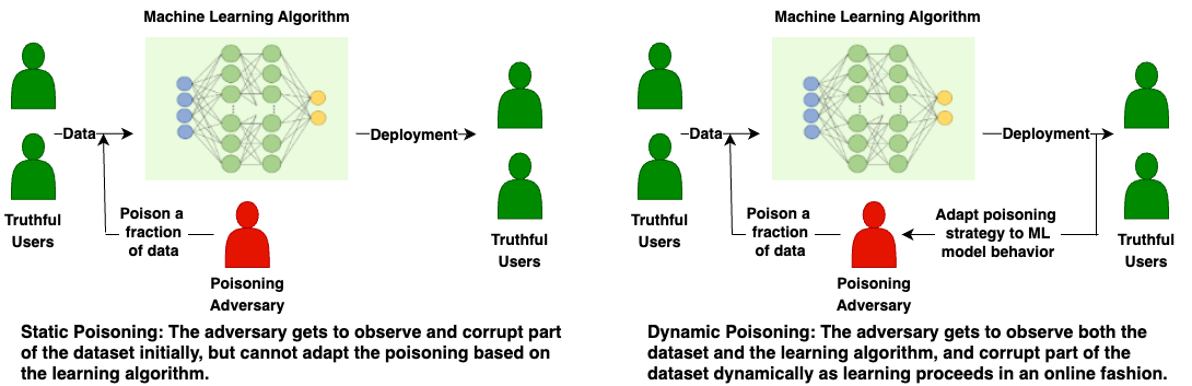
Figure 1: A schematic diagram to highlight the differences between static and dynamic poisoning.

1.1 Related Work

Data Poisoning.

Modern machine learning pipelines involve training on massive, uncurated datasets that are potentially untrustworthy and of such scale that conducting rigorous quality checks becomes impractical. Poisoning attacks (Biggio et al., 2012; Newsome et al., 2006; Biggio and Roli, 2018) pose big security concerns upon deployment of ML models. Depending on which stage (training / deployment) the poisoning takes place, they can be characterised as follows: 1. Static attacks: The model is trained on an offline dataset with poisoned data. Attacks could be untargeted, which aim to prevent training convergence rendering an unusable model and thus denial of service (Tian et al., 2022), or targeted, which are more task-specific and instead of simply increasing loss, attacks of this kind seeks to make the model output wrong predictions on specific tasks. 2. Backdoor attacks: In this setting, the test / deployment time data can be altered (Chen et al., 2017; Gu et al., 2017; Han et al., 2022; Zhu et al., 2019). Attackers manipulate a small proportion of the data such that, when a specific pattern / trigger is seen at test-time, the model returns a specific, erroneous prediction. 3. Dynamic (and adaptive) attacks: In scenarios where models are continuously/periodically updated in the face of new feedback, as is common in RLHF/fine tuning applications, a dynamic poisoning adversary Wang and Chaudhuri (2018); Zhang et al. (2020) can observe the behavior of the learning algorithm and adapt the poisoning in response.

Certified Poisoning Defense.

Recently, there have been works that attempt to achieve “certified robustness” to data poisoning, i.e., proving that the worst case impact of any poisoning strategy is below a certain bound that depends on parameters of the learning algorithm. All the work in this space, to the best of our knowledge, focuses on the static or backdoor attack adversary. (Steinhardt et al., 2017) provide certificates for linear models trained with gradient descent, (Rosenfeld et al., 2020) present a statistical upper-bound on the effectiveness of $\ell_{2}$ perturbations on training labels for linear models using randomized smoothing, (Zhang et al., 2022; Sosnin et al., 2024) present a model-agnostic certified approach that can effectively defend against both trigger-less and backdoor attacks, (Xie et al., 2022) observe that differential privacy, which usually covers addition or removal of data points, can also provide statistical guarantees in some limited poisoning settings. Even in (Wang and Feizi, 2024) which is the closest setting to our work, the poisoning adversary acts over offline datasets in a temporally extended fashion which are poisoned in one shot, and thus is not dynamic.

2 PROBLEM SETUP

We now develop the exact problem setup that we study in the paper. We consider a learning algorithm aimed at estimating parameters $\bm{\theta}\in\Theta$, and each step of the learning algorithm updates the estimates of these parameters based on potentially poisoned data. The following components fully define the problem setup. A notation table in provided in Appendix A.

Attack Type Adversary adapts poisoning Adversary can Certified strategy upon observing poison data robustness model behavior for deployed model Static / One-shot ✗ ✗ ✓ Backdoor ✗ ✓ ✓ Dynamic attack only ✓ ✓ ✗ Dynamic attack & defense (Ours) ✓ ✓ ✓

Table 1: A comparison with lines of work closest to ours. Static/One-shot ((Tian et al., 2022; Steinhardt et al., 2017; Rosenfeld et al., 2020)), Backdoor((Chen et al., 2017; Gu et al., 2017; Han et al., 2022; Zhu et al., 2019; Zhang et al., 2022; Sosnin et al., 2024)), Dynamic attack only (Wang and Chaudhuri (2018); Zhang et al. (2020).A detailed description is provided in Section 1.1.

Online learning algorithm.

We consider online learning algorithms that operate by receiving a new datapoint at each step and making an update to model parameters being estimated. In particular, we consider learning algorithms that can be written as

$$\bm{\theta}_{t+1}\leftarrow F_{\phi}\Bigl{(}\underbrace{\bm{\theta}_{t}}_{\text{Parameter}},\underbrace{{\bm{z}}_{t}}_{\text{Datapoint}}\Bigr{)},$$ (1)

where $F_{\phi}:{\bm{\Theta}}\times{\bm{Z}}\to{\bm{\Theta}}$ is a parameterized function that maps the current model parameters $\bm{\theta}_{t}$ to new model parameters $\bm{\theta}_{t+1}$, based on the received datapoint ${\bm{z}}_{t}$, where $\phi\in\bm{\Phi}$ is a hyperparameter, for example, learning rate in a gradient based learning algorithm, or strength of regularization used in the objective function.

Example To illustrate the setup we consider a simple toy example where we try to estimate the mean of the datapoints via gradient descent on the $\ell_{2}$ regularized squared Euclidean loss. Given a current estimate $\bm{\theta}_{t}$, upon receiving a datapoint ${\bm{z}}_{t}$, the update step can be written as:

$$\bm{\theta}_{t+1} =\bm{\theta}_{t}-\eta\nabla\bigl{(}\tfrac{1}{2}\|{\bm{z}}_{t}-\bm{\theta}_{t}\|_{2}^{2}+\tfrac{\sigma}{2}\|\bm{\theta}_{t}\|_{2}^{2}\bigr{)}$$

$$=(1-\eta-\eta\sigma)\bm{\theta}_{t}+\eta{\bm{z}}_{t}$$

$$=F_{\phi}(\bm{\theta}_{t},{\bm{z}}_{t}).$$

Here $\phi=\{\eta,\sigma\}$ denotes the learning rate and regularization parameter, and are the hyperparameters of the learning algorithm. Note that $F_{\phi}$ is a general update rule and we do not make any assumptions about $F_{\phi}$.

Poisoned learning algorithm.

We consider a setting where some of the data points received by the learning algorithm are corrupted by an adversary, who is allowed to choose corruptions as a function of the entire trajectory of the learning algorithm up to that point. We refer to such an adversary, who can observe the full trajectory and decide on the next corruption accordingly, as a dynamic adaptive adversary. While this may seem unrealistic, since our goal here is to compute certified bounds on the worst case adversary, we refrain from placing informational constraints on the adversary, as an adversary with sufficient side knowledge can still infer hidden parameters of the model from even from just a prediction API Tramèr et al. (2016).

The adversary is restricted to select a corrupted data point $\bm{z}^{\textup{adv}}_{t}\in\mathcal{A}$, which reflects constraints such as input feature normalization or the adversary trying to avoid outlier detection mechanisms used by the learner. We make no additional assumptions about the specific poisoning strategy employed by the adversary. Thus, our certificates of robustness to poisoning apply to any dynamic adaptive adversary who chooses poisoned data points from the set $\mathcal{A}$.

We assume that with a fixed probability, the data point the algorithm receives at each time step is poisoned. In practice, this could reflect the situation that out of a large population of human users providing feedback to a learning system, a small fraction are adversarial and will provide poisoned feedback. Let $\mathbb{P}^{\mathrm{data}}$ denote the benign distribution of data points. Mathematically, the data point ${\bm{z}}_{t}$ received by the learning algorithm at time $t$ is sampled according to ${\bm{z}}_{t}\sim\epsilon\delta(\bm{z}^{\textup{adv}}_{t})+(1-\epsilon)\mathbb{P}^{\mathrm{data}}$, where $\delta(\cdot)$ denotes the Dirac delta function, and $\epsilon$ is a parameter that controls the “level” of poisoning (analogous to the fraction of poisoned samples in static poisoning settings (Steinhardt et al., 2017)). This is a special case of Huber’s contamination model, which is used in the robust statistics literature (Diakonikolas and Kane, 2023) with the contamination model being a Dirac distribution. For compactness of the data generation process we define the following:

$$\mathbb{P}_{\epsilon}(\bm{z}^{\textup{adv}}):=\epsilon\delta(\bm{z}^{\textup{adv}})+(1-\epsilon)\mathbb{P}^{\mathrm{data}}.$$ (2)

2.1 Adversarial Objective

Transition Kernel.

Starting with a parameter estimate $\bm{\theta}$, the adversary chooses $\bm{z}^{\textup{adv}}$, then the learning algorithm updates the parameter estimate (via $F_{\phi}$). The transition kernel gives the probability (or probability density) that the parameter estimate assumes a value $\bm{\theta}^{\prime}$ after the above steps, and is defined as (recall that $\delta(\cdot)$ denotes the Dirac delta function):

$$\Pi(\bm{\theta}^{\prime}|\bm{\theta},\bm{z}^{\textup{adv}})=\operatorname*{\mathbb{E}}_{{\bm{z}}\sim\mathbb{P}_{\epsilon}(\bm{z}^{\textup{adv}})}\left[{\delta(F_{\phi}(\bm{\theta},{\bm{z}})-\bm{\theta}^{\prime})}\right].$$ (3)

Dynamics as a Markov Process.

The dynamics in Eq. (1) gives rise to a Markov process over the parameters $\bm{\theta}$. If $\mathbb{P}_{t}$ denotes the distribution over parameters at time $t$, we have

$$\mathbb{P}_{t+1}\left({\bm{\theta}^{\prime}}\right)=\int\Pi(\bm{\theta}^{\prime}|\bm{\theta},\bm{z}^{\textup{adv}})\mathbb{P}_{t}\left({\bm{\theta}}\right)d\bm{\theta}.$$ (4)

Since the learning algorithm (dynamics of the parameters) is a Markov process, the sequence of actions for the adversary (i.e., choices of $\bm{z}^{\textup{adv}}$) constitute a Markov Decision Process with

$$\underbrace{\bm{\theta}}_{\text{States}},\underbrace{\bm{z}^{\textup{adv}}}_{\text{Actions}},\underbrace{\Pi(\cdot|\bm{\theta},\bm{z}^{\textup{adv}})}_{\text{Transition Kernel}}.$$

Adversarial objective function.

We assume that the poisoning adversary is interested in maximizing some adversarial objective $\ell_{\textrm{adv}}:{\bm{\Theta}}\mapsto\mathbb{R}$, for example, the expected prediction error on some target distribution of interest to the adversary. The adversary wants to choose actions such that it can maximize its average reward over time. Utilizing the fact that the optimal policy for an MDP is stationary (i.e., the policy is time invariant), we define the adversary’s objective for an arbitrary stationary policy $\bm{z}^{\textup{adv}}\sim\pi(\cdot|\bm{\theta})$ as follows:

$$\rho(\pi)=\lim_{T\to\infty}\frac{1}{T}\operatorname*{\mathbb{E}}_{\pi}\left[{\sum_{t=1}^{T}\ell_{\textrm{adv}}(\bm{\theta}_{t})}\right],$$ (5)

where the expectation is with respect to the noisy state transition dynamics induced by the adversary’s poisoning policy $\pi$.

We utilize the fact that $\rho(\pi)$ is equal to the expected reward under the stationary state distribution (assuming the MDP is ergodic, see details in Appendix B):

$$\rho(\pi)=\operatorname*{\mathbb{E}}_{\bm{\theta}\sim d_{\pi}(\cdot)}\left[{\ell_{\rm adv}(\bm{\theta})}\right].$$

The stationary state is defined as a condition where the distribution of parameters remains unchanged over time. In other words, the distribution of parameters at any given point in the stationary state is identical to the distribution of parameters at the next state.

The stationarity condition can be expressed mathematically in terms of the transition kernel as:

$$\operatorname*{\mathbb{E}}_{\begin{subarray}{c}\bm{\theta}\sim d_{\pi}(\cdot)\\ \bm{z}^{\textup{adv}}\sim\pi(\cdot|\bm{\theta})\end{subarray}}\left[{\Pi(\bm{\theta}^{\prime}|\bm{\theta},\bm{z}^{\textup{adv}})}\right]=d_{\pi}(\bm{\theta}^{\prime})\quad\forall\bm{\theta}^{\prime}\in\Theta.$$

Given a family of learning algorithms $F_{\phi}$ with tunable parameters $\phi\in\bm{\Phi}$, our goal is to estimate $\phi$ so that our learning algorithm is robust to the poisoning as described above. However, since we assume that we are working in the online setting, it is seldom the case that we know the data distribution $\mathbb{P}^{\mathrm{data}}$ in advance, making the adversary’s objective intractable. In Section 2.2, we use a meta learning formulation to overcome the lack of knowledge about $\mathbb{P}^{\mathrm{data}}$ in advance.

2.2 Meta-learning a robust learning algorithm

In a meta learning setup (Hochreiter et al., 2001; Andrychowicz et al., 2016), we suppose that we have access to a meta-distribution from which data distributions can be sampled. In such a setup, we can “simulate” various data distributions and consider the following approach: We take a family of learning algorithms $F_{\phi}$ with tunable parameters $\phi\in\bm{\Phi}$, and attempt to design the parameters $\phi$ of the learning algorithm to trade-off performance and robustness in expectation over the data distributions sampled from the meta-distribution.

In particular, in the absence of poisoned data, the updates (1) on data sampled from benign data distribution $\mathbb{P}^{\mathrm{data}}$ result in a stationary distribution over model parameters $\bm{\theta}$ denoted by $\mathbb{P}\bigl{(}\phi,\mathbb{P}^{\mathrm{data}}\bigr{)}$. The expected benign target loss can be written as :

$$b(\phi,\mathbb{P}^{\mathrm{data}})=\operatorname*{\mathbb{E}}_{\bm{\theta}\sim\mathbb{P}\left({\phi,\mathbb{P}^{\mathrm{data}}}\right)}\left[{\ell\left({\bm{\theta}}\right)}\right],$$ (6)

where $\ell:{\bm{\Theta}}\mapsto\mathbb{R}$ is the loss the learning algorithm wants to minimize.

In Section 2.3, we propose a general formulation to derive an upper bound on the worst case impact of an adversary on the target loss (a certificate), which we denote by $c(\phi,\mathbb{P}^{\mathrm{data}})$ for a given data distribution $\mathbb{P}^{\mathrm{data}}$ and parameter of the learning algorithm $\phi\in\bm{\Phi}$.

Given a meta distribution $\mathcal{P}$, we can propose the following criterion to design a robust learning algorithm:

$$\inf_{\phi\in\bm{\Phi}}\mathbb{E}_{\mathbb{P}^{\mathrm{data}}\sim\mathcal{P}}\bigg{[}b(\phi,\mathbb{P}^{\mathrm{data}})+\kappa\cdot c(\phi,\mathbb{P}^{\mathrm{data}})\bigg{]}.$$ (7)

where $\kappa>0$ is a trade-off parameter. The expectation over $\mathcal{P}$ is a meta-learning inspired formulation, where we are designing a learning algorithm that is good “in expectation” under a meta-distribution over data distributions. The first term constitutes “doing well” in the absence of the adversary by converging to a stationary distribution over parameters that incurs low expected loss. The second term is an upper bound on the worst case loss incurred by the learning algorithm in the presence of the adversary.

2.3 Technical Approach: Certificate of Robustness

For a given $\mathbb{P}^{\mathrm{data}}\sim\mathcal{P}$, we attempt to find an upper bound on the worst case impact of the adversary. Recalling that the sequence of actions for the adversary constitutes a Markov Decision Process, the value of the adversarial objective for the adversary’s optimal action sequence is therefore the average reward in the infinite horizon Markov Decision Process setting (Malek et al., 2014) and can be written as the solution of an infinite dimensional linear program (LP) Puterman (2014). The LP can be written as:

$$\sup_{\begin{subarray}{c}d_{\pi}\in\mathcal{P}[{\bm{\Theta}}]\\ \pi\in\mathcal{P}[{\bm{\Theta}}\times{\bm{Z}}]\end{subarray}}\quad\operatorname*{\mathbb{E}}_{\bm{\theta}\sim d_{\pi}(\cdot)}\left[{\ell_{\textup{adv}}\left({\bm{\theta}}\right)}\right],\quad\text{subject to }$$ (8)

$$\operatorname*{\mathbb{E}}_{\begin{subarray}{c}\bm{\theta}\sim d_{\pi}(\cdot)\\ \bm{z}^{\textup{adv}}\sim\pi(\cdot|\bm{\theta})\end{subarray}}\left[{\Pi(\bm{\theta}^{\prime}|\bm{\theta},\bm{z}^{\textup{adv}})}\right]=d_{\pi}(\bm{\theta}^{\prime})\quad\forall\bm{\theta}^{\prime}\in\Theta,$$

where $\mathcal{P}[{\bm{\Theta}}]$, $\mathcal{P}[{\bm{\Theta}}\times{\bm{Z}}]$ denote the space of probability measures on ${\bm{\Theta}}$ and ${\bm{\Theta}}\times{\bm{Z}}$ respectively.

We are now ready to present our certificate of robustness against dynamic data poisoning adversaries, which is the largest objective value any dynamic adversary can attain in the stationary state.

Theorem 1.

For any function $\lambda:\Theta\mapsto\mathbb{R}$, for any dynamic adaptive adversary, the average loss (5) is bounded above by

$$\sup_{\begin{subarray}{c}\bm{\theta}\in{\bm{\Theta}}\\ \bm{z}^{\textup{adv}}\in\mathcal{A}\end{subarray}}\quad\operatorname*{\mathbb{E}}_{\bm{\theta}^{\prime}\sim\Pi(\cdot|\bm{\theta},\bm{z}^{\textup{adv}})}\left[{\lambda\left({\bm{\theta}^{\prime}}\right)}\right]+\ell_{\textup{adv}}\left({\bm{\theta}}\right)-\lambda\left({\bm{\theta}}\right).$$ (9)

Proof.

Follows by weak duality for the LP (8). Detailed proof in Appendix B. ∎

If strong duality holds Nash and Anderson (1987); Clark (2003), we further have that the optimal value of (8) is exactly equal to

$$\hskip-13.00806pt{{\inf_{\lambda:{\bm{\Theta}}\mapsto\mathbb{R}}\sup_{\begin{subarray}{c}\bm{\theta}\in{\bm{\Theta}}\\ \bm{z}^{\textup{adv}}\in\mathcal{A}\end{subarray}}\operatorname*{\mathbb{E}}_{\bm{\theta}^{\prime}\sim\Pi(\cdot|\bm{\theta},\bm{z}^{\textup{adv}})}\left[{\lambda\left({\bm{\theta}^{\prime}}\right)}\right]+\ell_{\textup{adv}}\left({\bm{\theta}}\right)-\lambda\left({\bm{\theta}}\right).}}$$ (10)

3 MEAN ESTIMATION

Consider the mean estimation problem, where we aim to learn the parameter $\bm{\theta}\in\mathbb{R}^{d}$ to estimate the mean $\mu=\operatorname*{\mathbb{E}}_{{\bm{z}}\sim\mathbb{P}^{\mathrm{data}}}\left[{{\bm{z}}}\right]$ of a distribution $\mathbb{P}^{\mathrm{data}}$. Given a data point ${\bm{z}}_{t}$, the learning rule is given by:

$$\bm{\theta}_{t+1}\leftarrow(1-\eta)\bm{\theta}_{t}+\eta{\bm{z}}_{t}+\eta{\bm{B}}{\bm{w}}_{t},$$ (11)

where $\eta$ is the learning rate, ${\bm{S}}={\bm{B}}{\bm{B}}^{\top}\in\mathbb{S}^{d}_{+}$ is the tunable defense hyperparameter and ${\bm{w}}_{t}\sim\mathcal{N}(0,{\bm{I}})$ is Gaussian noise. The adversary wants to maximize its average reward according to the following objective function:

$$\ell_{\textup{adv}}\left({\bm{\theta}}\right)=\|\mu-\bm{\theta}\|^{2}.$$ (12)

Certificate on adversarial loss (analysis).

Theorem 2.

Choosing $\lambda:\mathbb{R}^{d}\rightarrow\mathbb{R}$ in Theorem 1 to be quadratic, i.e. $\lambda\left({\bm{\theta}}\right)=\bm{\theta}^{\top}{\bm{A}}\bm{\theta}+\bm{\theta}^{\top}{\bm{b}}$, the adversarial constraint set of the form $\|\bm{z}^{\textup{adv}}-\mu\|_{2}^{2}\leq r$, the certificate for the mean estimation problem for $\mathbb{P}^{\mathrm{data}}({\bm{z}})=\mathcal{N}({\bm{z}}|\mu,\bm{\varSigma})$ for a fixed learning algorithm (i.e. ${\bm{S}}$ is fixed) is given by:

$$\inf_{{\bm{A}}\in\mathbb{S}^{d},{\bm{b}}\in\mathbb{R}^{d},\nu\geq 0}g({\bm{A}},{\bm{b}},\nu,{\bm{S}},\mu,\bm{\varSigma}),$$ (13)

where $g({\bm{A}},{\bm{b}},\nu,{\bm{S}},\mu,\bm{\varSigma})$ is a convex objective in ${\bm{A}},{\bm{b}},\nu$ as defined below:

$$\begin{cases}\frac{1}{4}\left\|\begin{bmatrix}2(1-\epsilon)\eta(1-\eta){\bm{A}}\mu-2\mu-\eta{\bm{b}}\\ \epsilon\eta{\bm{b}}+2\nu\mu\end{bmatrix}\right\|^{2}_{{\bm{D}}}\\ \;\;+(1-\epsilon)(\eta^{2}\operatorname{Trace}(\bm{\varSigma}{\bm{A}})+\eta^{2}\mu^{\top}{\bm{A}}\mu+\eta{\bm{b}}^{\top}\mu)\hskip-8.53581pt\\ \qquad+\mu^{\top}\mu+\eta^{2}\operatorname{Trace}({\bm{A}}{\bm{S}})+\nu(r-\mu^{\top}\mu),\\ \qquad\qquad\text{if }\nu\geq 0\text{ and }{\bm{D}}\succeq 0\\ -\infty\qquad\;\text{otherwise,}\end{cases}$$ (14)

where ${\bm{D}}=\begin{bmatrix}(1-(1-\eta)^{2}){\bm{A}}-{\bm{I}}&-\eta\epsilon(1-\eta){\bm{A}}\\ -\eta\epsilon(1-\eta){\bm{A}}&-\epsilon\eta^{2}{\bm{A}}-\nu{\bm{I}}\end{bmatrix}$ and $\|{\bm{x}}\|^{2}_{{\bm{D}}}={\bm{x}}^{\top}{\bm{D}}^{-1}{\bm{x}}$.

Proof.

The detailed proof can be found in Appendix C. The proof sketch follows by noting that for a fixed $\lambda$ the dual of the inner constrained maximization problem is a quadratic expression in $\bm{z}^{\textup{adv}},\bm{\theta}$ and a finite supremum exists if the Hessian is negative semidefinite (which leads to the $\mathbf{D}\succeq 0$ constraint). Plugging in the maximizer we get a minimization problem in the dual variables $\nu$. Finally we note that the overall minimization problem is jointly convex in ${\bm{A}},{\bm{b}},\nu$. ∎

Remark 3.1.

The problem above is a convex problem since it has a matrix fractional objective function Boyd and Vandenberghe (2004) with a Linear Matrix Inequality (LMI) constraint.

Meta-Learning Algorithm.

Following the formulation in Eq. (7), we wish to learn a defense parameter ${\bm{S}}$ that minimizes the expected loss (expectation over different $\mathbb{P}^{\mathrm{data}}$ from the meta distribution $\mathcal{P}$). For the mean estimation problem this boils down to solving

$$\inf_{\begin{subarray}{c}{\bm{S}}\in\mathbb{S}^{d}_{+}\end{subarray}} \eta^{2}\operatorname{Trace}({\bm{S}})+\kappa\mathbb{E}_{\mu,\bm{\varSigma}\sim\mathcal{P}}[\!\!\!\!\inf_{\begin{subarray}{c}\nu\geq 0\\ {\bm{A}}\in\mathbb{S}^{d},{\bm{b}}\in\mathbb{R}^{d}\end{subarray}}\!\!\!\!g({\bm{A}},{\bm{b}},\nu,{\bm{S}},\mu,\bm{\varSigma})].$$ (15)

Remark 3.2.

Note that problem (15) is not jointly convex in ${\bm{S}},{\bm{A}},{\bm{b}},\nu$ because of the $\operatorname{Trace}({\bm{A}}{\bm{S}})$ term in $g$; see (14). However, it is convex individually in ${\bm{S}}$ and $\{{\bm{A}},{\bm{b}},\nu\}$. We use an alternating minimization approach to seek a local minimum of problem (15), as detailed in Algorithm 1.

In practice, one observes a finite number of distributions from $\mathcal{P}$, and sample average approximation is leveraged, with the aim of learning a defense parameter which generalizes well to unseen distributions from $\mathcal{P}$. This process is stated in Algorithm 1.

Algorithm 1 Meta learning a robust learning algorithm for mean estimation

1: Input: Set of $K$ distributions $\{\mathcal{N}(\mu_{i},\bm{\varSigma}_{i})\}_{i\in[K]}$ sampled from $\mathcal{P}[\mathbb{P}^{\mathrm{data}}]$, tradeoff parameter $\kappa$, and max iterations $T$.

2: Initialize: ${\bm{S}}^{(1)}\in\mathbb{S}^{d}_{+}$ randomly.

3: Alternating Minimization over Lagrange multipliers $\{{\bm{A}}_{i},{\bm{b}}_{i},\nu_{i}\}_{i\in[K]}$ and defense parameter ${\bm{S}}$.

4: for $t=1,\ldots,T$ do

5:  for $i=1,\ldots,K$ do

6:   ${\bm{A}}_{i},{\bm{b}}_{i},\nu_{i}=\underset{{\bm{A}}\in\mathbb{S}^{d},{\bm{b}}\in\mathbb{R}^{d},\nu\geq 0}{\operatorname*{\mathrm{argmin}}}g({\bm{A}},{\bm{b}},\nu,{\bm{S}}^{(t)},\mu_{i},\bm{\varSigma}_{i})$

7:  end for

8:  ${\bm{S}}^{(t+1)}=\underset{{\bm{S}}\in\mathbb{S}^{d}_{+}}{\operatorname*{\mathrm{argmin}}}\bigl{(}\frac{\kappa}{K}\sum_{i\in[K]}g({\bm{A}}_{i},{\bm{b}}_{i},\nu_{i},{\bm{S}},\mu_{i},\bm{\varSigma}_{i})$                $+\eta^{2}\operatorname{Trace}({\bm{S}})\bigr{)}$

9: end for

10: return  ${\bm{S}}^{(T+1)}$

4 BINARY CLASSIFICATION

We consider the binary classification problem. Given an input feature ${\bm{x}}\in\mathbb{R}^{d}$ such that $\|{\bm{x}}\|_{2}\leq 1$, a linear predictor $\bm{\theta}\in\mathbb{R}^{d}$ tries to predict the label $y\in\{-1,1\}$ via the sign of $\bm{\theta}^{\top}{\bm{x}}$ . To define the losses, we introduce ${\bm{z}}=y{\bm{x}}\in\mathbb{R}^{d}$ which is the label multiplied by the feature and note that $\|{\bm{z}}\|_{2}\leq 1$.

A dynamic adversary tries to corrupt samples so that the learning algorithm learns a $\bm{\theta}$ that maximizes the hinge loss on a target distribution $\mathbb{P}^{\mathrm{target}}$, captured by the following objective:

$$\ell_{\textrm{adv}}(\bm{\theta})=\operatorname*{\mathbb{E}}_{z\sim\mathbb{P}^{\mathrm{target}}}\left[{\max\{0,1-\bm{\theta}^{\top}{\bm{z}}\}}\right].$$ (16)

The learning algorithm tires to minimize the regularized hinge loss on the observed datapoints:

$$l(\bm{\theta},{\bm{z}}) =\max\{0,1-\bm{\theta}^{\top}{\bm{z}}\}+\frac{\sigma}{2}\|\bm{\theta}\|_{2}^{2}.$$ (17)

Upon observing a sample ${\bm{z}}_{t}$, the parameter is updated via a gradient descent: $\bm{\theta}_{t+1}=F(\bm{\theta}_{t},{\bm{z}}_{t})$, where

$$F(\bm{\theta},{\bm{z}}) =\bm{\theta}_{t}-\eta\nabla_{\bm{\theta}}l(\bm{\theta}_{t},{\bm{z}}_{t})$$

$$=(1-\sigma\eta)\bm{\theta}+\eta\mathbb{I}[\bm{\theta}^{\top}{\bm{z}}\leq 1]{\bm{z}}.$$ (18)

Below, we provide a certificate for the adversarial objective at stationarity of this learning algorithm.

Theorem 3.

Choosing $\lambda:\mathbb{R}^{d}\rightarrow\mathbb{R}$ in Theorem 1 to be quadratic, i.e., $\lambda\left({\bm{\theta}}\right)=\bm{\theta}^{\top}{\bm{A}}\bm{\theta}+{\bm{b}}^{\top}\bm{\theta}$, parameter space ${\bm{\Theta}}=\{\bm{\theta}\mid\|\bm{\theta}\|_{2}\leq\frac{1}{\sigma}\}$ and the adversarial constraint set of the form $\mathcal{A}=\{\bm{z}^{\textup{adv}}\mid\|\bm{z}^{\textup{adv}}\|_{2}\leq 1\}$, the certificate for the binary classification problem for $\mathbb{P}^{\mathrm{data}}({\bm{z}})=\{{\bm{z}}_{1},\ldots,{\bm{z}}_{N}\}$ for a learning algorithm with regularization parameter $\sigma$, and learning rate $\eta$ is upper bounded by

$$\max\left(\textup{\sf OPT}_{1},\textup{\sf OPT}_{2}\right)$$

$$\textup{\sf OPT}_{1}=\inf_{\nu,{\bm{A}},{\bm{b}}}\quad \|{\bm{p}}({\bm{b}},\nu)\|^{2}_{{\bm{D}}({\bm{A}},\nu)^{-1}}+q(\nu)$$

s.t. $${\bm{D}}({\bm{A}},\nu)\succeq 0,$$

$${\bm{r}}_{i}(\nu)+{\bm{s}}(z_{i},{\bm{A}},{\bm{b}})=0,\;\;\forall i\in[N].$$

$$\textup{\sf OPT}_{2}=\inf_{\nu,{\bm{A}},{\bm{b}}}\quad \|{\bm{p}}^{\prime}({\bm{b}},\nu)\|^{2}_{{\bm{D}}^{\prime}({\bm{A}},\nu)^{-1}}+q^{\prime}(\nu)$$

s.t. $${\bm{D}}^{\prime}({\bm{A}},\nu)\succeq 0,$$

$${\bm{r}}_{i}(\nu)+{\bm{s}}(z_{i},{\bm{A}},{\bm{b}})=0,\;\;\forall i\in[N].$$

where ${\bm{p}}()$, ${\bm{p}}^{\prime}()$, $q()$, $q^{\prime}()$, ${\bm{D}}()$, ${\bm{D}}^{\prime}()$, ${\bm{r}}_{1}(),\ldots,{\bm{r}}_{N}()$, ${\bm{s}}()$ are affine functions of the optimization variables $\nu,{\bm{A}},{\bm{b}}$ as defined below and $\nu=\{\nu_{1},\ldots,\nu_{10}\}$:

$${\bm{p}}({\bm{b}},\nu) =\frac{1}{2}\begin{bmatrix}-\sigma\eta{\bm{b}}+\sum_{i\in[N]}\left((\nu_{1i}-\nu_{2i}){\bm{z}}_{i}-\nu_{4i}+\nu_{6i}\right)\\ \epsilon\eta{\bm{b}}\end{bmatrix},$$

$${\bm{D}}({\bm{A}},\nu) =\begin{bmatrix}[1-(1-\sigma\eta)^{2}]{\bm{A}}+\nu_{8}{\bm{I}}&-\epsilon(1-\sigma\eta)\eta{\bm{A}}+\nu_{9}{\bm{I}}\\ -\epsilon(1-\sigma\eta)\eta{\bm{A}}+\nu_{9}{\bm{I}}&-\epsilon\eta^{2}{\bm{A}}+\nu_{10}{\bm{I}}\end{bmatrix},$$

$$q(\nu) =q^{\prime}(\nu)+2\nu_{9}+\nu_{10},$$

$${\bm{p}}^{\prime}({\bm{b}},\nu) =\frac{1}{2}\begin{bmatrix}-\sigma\eta{\bm{b}}+\sum_{i\in[N]}\left((\nu_{1i}-\nu_{2i}){\bm{z}}_{i}-\nu_{4i}+\nu_{6i}\right)\end{bmatrix},$$

$${\bm{D}}^{\prime}({\bm{A}},\nu) =[1-(1-\sigma\eta)^{2}]{\bm{A}}+\nu_{8}{\bm{I}},$$

$$q^{\prime}(\nu) =-\nu_{1}^{\top}\mathbf{1}+(2+\tfrac{1}{\sigma})\nu_{2}^{\top}\mathbf{1}+\tfrac{(\nu_{4}+\nu_{6})^{\top}\bf 1}{\sigma}+\mathbf{1}^{\top}\nu_{7}+\frac{\nu_{8}}{\sigma^{2}},$$

$${\bm{r}}_{i}(\nu) =\begin{bmatrix}(1+\frac{1}{\sigma})(\nu_{1i}-\nu_{2i})-\frac{\mathbf{1}^{\top}(\nu_{4i}+\nu_{6i})}{\sigma}-\nu_{7i}\\ \nu_{3i}+\nu_{4i}-\nu_{5i}-\nu_{6i}\end{bmatrix},$$

$${\bm{s}}({\bm{z}}_{i},{\bm{A}},{\bm{b}}) =\frac{1}{N}\begin{bmatrix}(1-\epsilon)\eta^{2}{\bm{z}}_{i}^{\top}{\bm{A}}{\bm{z}}_{i}+(1-\epsilon)\eta{\bm{b}}^{\top}{\bm{z}}_{i}+1\\ 2(1-\epsilon)\eta(1-\sigma\eta){\bm{A}}{\bm{z}}_{i}-{\bm{z}}_{i}\end{bmatrix}.$$

Proof.

A detailed derivation can be found in the Appendix D. The proof steps are: (i) Regularization implicitly bounds the decision variable $\bm{\theta}\in{\bm{\Theta}}$ without the need for projections, (ii) Considering 2 cases for the indicator term of $\bm{z}^{\textup{adv}}$ and taking the maximum of these 2 cases, (iii) Relaxing the indicator terms for benign samples into continuous variables between $[0,1]$, and (iv) Using McCormick relaxations (Mitsos et al., 2009) to convexify the bilinear terms in the objective. ∎

Extension to Multi-Class Setting: Our analysis can be extended to the multi-class classification setting. Let us consider score based classifiers, where $\Theta=\{\theta_{1},\ldots,\theta_{K}\}\in\mathbb{R}^{d}$ are the learnable parameters and the class prediction for a feature $x\in\mathbb{R}^{d}$ is given by $\arg\max_{i\in[K]}\theta_{i}^{\top}x$.

The SVM loss for any arbitrary feature $x$ with label $y$ is defined as: $\ell(\Theta,(x,y))=\sum_{j\neq y}\max\{0,1+(\theta_{j}-\theta_{y})^{\top}x\}$

The gradient update takes the form: $F(\theta_{y},(x,y))=\theta_{y}+\eta\sum_{j\neq y}\mathbb{I}[1+(\theta_{j}-\theta_{y})^{\top}x>0]x$ and for all $j\neq y$, we have $F(\theta_{j},(x,y))=\theta_{j}-\eta\mathbb{I}[1+(\theta_{j}-\theta_{y})^{\top}x>0]x$.

Note that the non-linearity in both the loss function and the update is composed with a linear combination of the parameters (i.e. $\theta_{j}-\theta_{y}$), and thus the analysis in the proof of Theorem 3 still holds, and our analysis for the binary classification generalizes to the multi-class classification.

5 EXPERIMENTS

We conduct experiments on both synthetic and real data to empirically validate our theoretical tools.

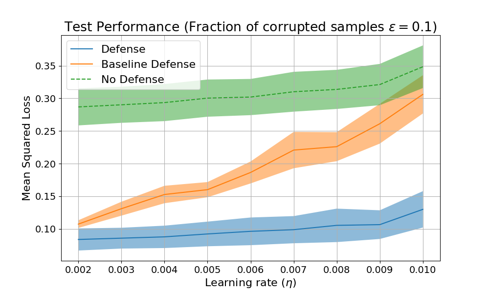
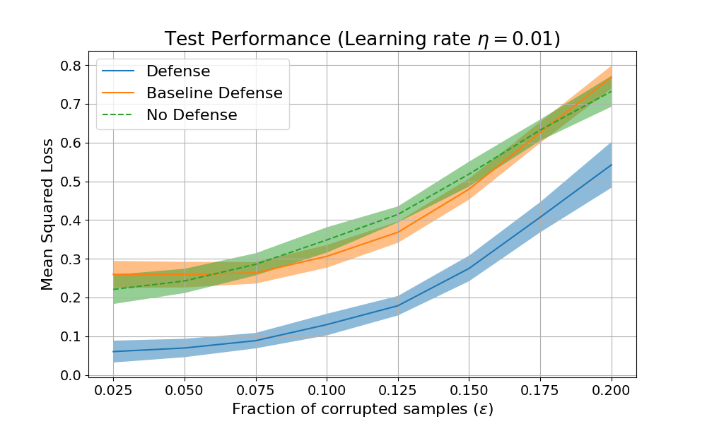
Figure 2: Test performance (mean squared error between true and estimated means) upon varying the learning rates (above) and the the fraction of samples corrupted by the dynamic adversary (below) and observed that our defense significantly outperforms training without defense.

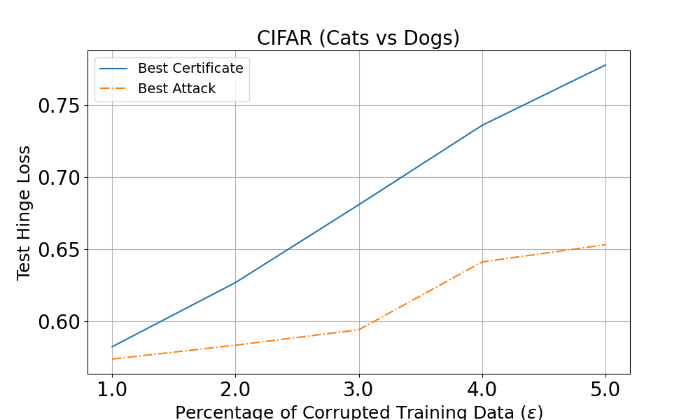
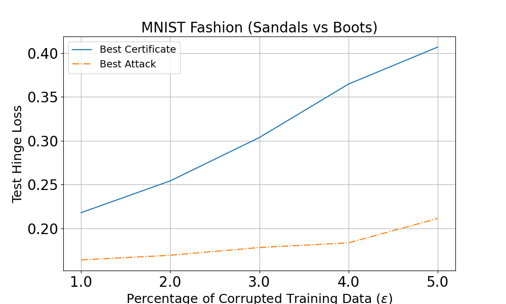
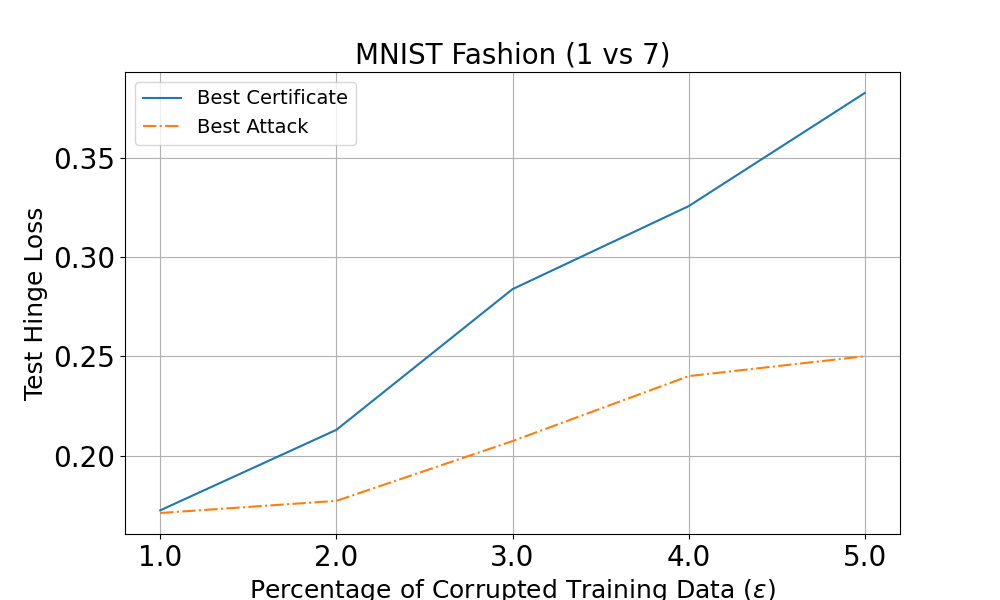
Figure 3: We plot the certificates of robustness for various settings (hyperparameter values) which act as upper bounds on the optimal dynamic adversary’s objective. We also plot the test losses on the adversarial objective for various attacks which act as lower bounds on the objective of the optimal adversary.

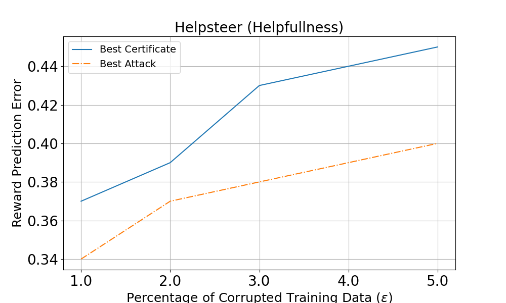
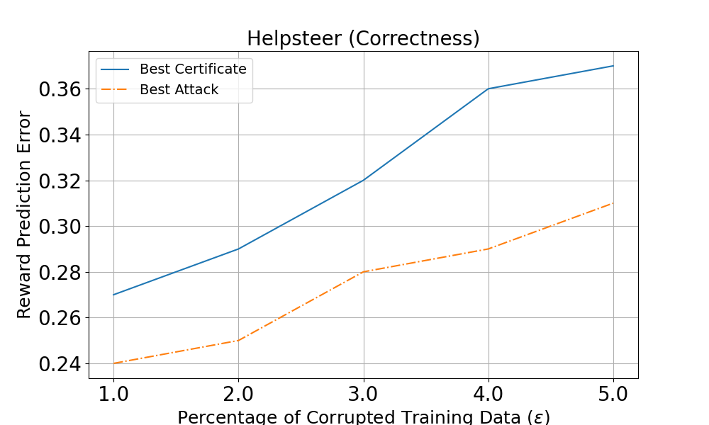
Figure 4: Poor choice of hyperparameters of the learning algorithm can make them vulnerable to dynamic attackers as noted by our certificates and attacks (red plots). Lower values of certificate, indicate more robust learning algorithms (blue, orange, green plots).

5.1 Mean Estimation

We wish to evaluate the robustness of our meta learning algorithm in Eq. (7) to design a defense against a dynamic best responding adversary on a ($d=20$) mean estimation task. We consider 3 different learning algorithms: 1. No Defense: Eq. (11) with ${\bm{B}}=\mathbf{0}$, i.e. no additive Gaussian noise, 2. Baseline Defense: ${\bm{B}}$ in Eq. (11) is restricted to be Isotropic Gaussian, 3. Defense: ${\bm{B}}$ in Eq. (11) can be arbitrarily shaped. We use Algorithm 1 to compute the defense parameter ${\bm{S}}={\bm{B}}{\bm{B}}^{\top}$ for the latter 2 learning algorithms by training on 10 randomly chosen Gaussians drawn from standard Gaussian prior for the mean and standard Inverse Wishart prior for the covariance. We report the average test performance on 50 Gaussian distributions drawn from the same prior (see Figure 2).

5.2 Image Classification

We consider binary classification tasks on multiple datasets : (i) MNIST (Deng, 2012), (ii) FashionMNIST (Xiao et al., 2017), (iii) CIFAR-10(Krizhevsky et al., 2009). Detailed dataset descriptions and preprocessing steps can be found in Appendix E.

In our experiments, we choose $\mathbb{P}^{\mathrm{target}}$ in Eq. (16) to be the same as $\mathbb{P}^{\mathrm{data}}$, i.e., the adversary’s objective is to make the model perform poorly on the benign data distribution.

To learn the hyperparameters for a robust online learning algorithm (Eq. (18)), we adopt the Meta learning setup presented in Eq. (7). We choose $\mathcal{P}$ as a set of binary classification datasets on label pairs different from the label pair the online algorithm receives data from. For example, we use data from MNIST: 4 vs 9, 5 vs 8, 3 vs 8, 0 vs 6 to construct the objective in Eq. (7) and then test the performance of the onlne learning algorithm with the learnt hyperparameters on MNIST: 1 vs 7 (see Appendix E for more details). We compute certificates for different fractions of the training data to be corrupted $\epsilon\in\{1\%,2\%,3\%,4\%,5\%\}$, and vary $\eta,\sigma$ for various values of $\eta$ and $\sigma$ by performing a grid search over $\eta\in\{5\times 10^{-5},1\times 10^{-4},5\times 10^{-4},1\times 10^{-3},5\times 10^{-3}\}$ and $\sigma\in\{3\times 10^{-3},6\times 10^{-3},1\times 10^{-2},3\times 10^{-2},6\times 10^{-2}\}$. We tune the hyperparameter $\kappa$ in Eq. (7) to trade off benign loss and robustness certificate by the generalization test loss on a held-out validation set. In Figure 3 we plot the certificates of robustness corresponding to hyperparameters $(\eta,\sigma)$ pairs having smallest objective values in Eq. (7).

Additionally, we evaluate the learning algorithm against three types of attacks: 1. fgsm: The attacker, having access to model parameters at each time step, initializes a random $\mathbf{z}_{\text{adv}}$, computes the gradient of $\bm{z}^{\textup{adv}}$ on the adversarial loss, takes a gradient ascent step on $\bm{z}^{\textup{adv}}$ and projects the result onto the unit $\ell_{2}$ ball, 2. pgd: similar to fgsm, but instead of a single big gradient step, the attacker takes multiple small steps and projects onto the unit $\ell_{2}$ ball, 3. label flip: the attacker picks an arbitrary data point and flips its label. In Figure 3, we plot the best attack (corresponding to largest prediction error) for each value of $\epsilon$. We observe the following: The test adversarial loss under different heuristic attacks is consistently lower than the computed robustness certificate.

5.3 Reward Learning

We conduct reward learning experiments using Helpsteer, an open-source helpfulness dataset that is used to align large language models to become more helpful, factually correct and coherent, while being adjustable in terms of the complexity and verbosity of its responses (Wang et al., 2023; Dong et al., 2023). Since the datasets of human feedback, both for open source and closed sourced models, are typically composed of users ‘in the wild‘ using the model, there is potential for adversaries to introduce poisoning. This can lead to the learned reward model favoring specific demographic groups, political entities or unscientific points of view, eventually leading to bad and potentially harmful experiences for users of language models fine tuned on the learned reward.

To apply our framework to this problem, we consider a simple reward model. Given a (prompt, response) pair, we extract a feature representation ${\bm{x}}$ using a pretrained BERT model, and our reward model parameterized by $\bm{\theta}$, predicts the reward as $\bm{\theta}^{\top}{\bm{x}}$. Given the score $y$ (normalised to fall within the range $[-1,1]$) on a particular attribute (say helpfulness), the learning algorithm proceeds to learn the reward model by performing gradient descent on the regularized hinge loss objective Eq. (17). We follow the similar hyperprameter search space as the image classification example using the meta learning setup in Eq. (7). The results for helpfulness and correctness are presented in Figure 4. More details are deferred to Appendix E.

6 CONCLUSION AND FUTURE WORK

This paper presents a novel framework for computing certified bounds on the worst-case impacts of dynamic data poisoning adversaries in machine learning. This framework lays the groundwork for developing robust algorithms, which we demonstrate for mean estimation and linear classifiers. Extending this framework to efficient algorithms for more general learning setups, particularly deep learning setups that use human feedback with potential for malicious feedback, would be a compelling direction of future work. Furthermore, considering alternative strategies for computing the bound in (9), particularly ones driven by AI advances, would be a promising approach for scaling. Recent work has demonstrated that AI systems can be used to discover Lyapunov functions for dynamical systems (Alfarano et al., 2023), indicating that AI driven approaches could hold promise in this setting.

Appendix A Notations

Notation	Interpretation	Belongs to
$F_{\phi}^{d}$$\bm{\theta}$	Model Parameters	${\bm{\Theta}}$
$F_{\phi}^{d}$$\bm{\phi}$	Hyper-parameters	$\bm{\Phi}$
$F_{\phi}^{d}$${\bm{z}}$	Data point	${\bm{Z}}$
$F_{\phi}^{d}$$F_{\phi}$	Update rule	${\bm{\Theta}}\times{\bm{Z}}\mapsto{\bm{\Theta}}$
$F_{\phi}^{d}$$\bm{z}^{\textup{adv}}$	Adversarial data point	$\mathcal{A}$
$F_{\phi}^{d}$$\ell_{\rm adv}$	Adversarial objective fn.	${\bm{\Theta}}\mapsto\mathbb{R}$
$F_{\phi}^{d}$$\mathbb{P}^{\mathrm{data}}$	Benign Data Dist.	$\mathcal{P}[{\bm{Z}}]$
$F_{\phi}^{d}$$\Pi(\cdot|\bm{\theta},\bm{z}^{\textup{adv}})$	State Transition Kernel	${\bm{\Theta}}\!\times\!{\bm{Z}}\mapsto\mathcal{P}[{\bm{\Theta}}]$​​

Table 2: Notation.

Appendix B Proofs

See 1

Proof.

The primal problem is defined below:

$$\sup_{\begin{subarray}{c}d_{\pi}\in\mathcal{P}[{\bm{\Theta}}]\\ \pi\in\mathcal{P}[{\bm{\Theta}}\times{\bm{Z}}]\end{subarray}}\quad\operatorname*{\mathbb{E}}_{\bm{\theta}\sim d_{\pi}(\cdot)}\left[{\ell_{\textup{adv}}\left({\bm{\theta}}\right)}\right],\quad\text{subject to }$$

$$\operatorname*{\mathbb{E}}_{\begin{subarray}{c}\bm{\theta}\sim d_{\pi}(\cdot)\\ \bm{z}^{\textup{adv}}\sim\pi(\cdot|\bm{\theta})\end{subarray}}\left[{\Pi(\bm{\theta}^{\prime}|\bm{\theta},\bm{z}^{\textup{adv}})}\right]=d_{\pi}(\bm{\theta}^{\prime})\quad\forall\bm{\theta}^{\prime}\in\Theta.$$

For a given function $\lambda:{\bm{\Theta}}\mapsto\mathbb{R}$, the Lagrangian can be written as:

$$\mathcal{L}(d_{\pi},\pi,\lambda) =\operatorname*{\mathbb{E}}_{\bm{\theta}\sim d_{\pi}(\cdot)}\left[{\ell_{\textup{adv}}\left({\bm{\theta}}\right)}\right]+\int_{\bm{\theta}^{\prime}\in{\bm{\Theta}}}\lambda(\bm{\theta}^{\prime})\bigg{[}\operatorname*{\mathbb{E}}_{\begin{subarray}{c}\bm{\theta}\sim d_{\pi}(\cdot)\\ \bm{z}^{\textup{adv}}\sim\pi(\cdot|\bm{\theta})\end{subarray}}\left[{\Pi(\bm{\theta}^{\prime}|\bm{\theta},\bm{z}^{\textup{adv}})}\right]-d_{\pi}(\bm{\theta}^{\prime})\bigg{]}d\bm{\theta}^{\prime}$$

$$=\operatorname*{\mathbb{E}}_{\bm{\theta}\sim d_{\pi}(\cdot)}\left[{\ell_{\textup{adv}}\left({\bm{\theta}}\right)}\right]+\operatorname*{\mathbb{E}}_{\begin{subarray}{c}\bm{\theta}\sim d_{\pi}(\cdot)\\ \bm{z}^{\textup{adv}}\sim\pi(\cdot|\bm{\theta})\end{subarray}}\left[{\operatorname*{\mathbb{E}}_{\bm{\theta}^{\prime}\sim\Pi(\cdot|\bm{\theta},\bm{z}^{\textup{adv}})}\left[{\lambda(\bm{\theta}^{\prime})}\right]}\right]-\operatorname*{\mathbb{E}}_{\bm{\theta}^{\prime}\sim d_{\pi}(\cdot)}\left[{\lambda(\bm{\theta}^{\prime})}\right]$$

$$=\operatorname*{\mathbb{E}}_{\begin{subarray}{c}\bm{\theta}\sim d_{\pi}(\cdot)\\ \bm{z}^{\textup{adv}}\sim\pi(\cdot|\bm{\theta})\end{subarray}}\left[{\operatorname*{\mathbb{E}}_{\bm{\theta}^{\prime}\sim\Pi(\cdot|\bm{\theta},\bm{z}^{\textup{adv}})}\left[{\lambda(\bm{\theta}^{\prime})}\right]+\ell_{\textup{adv}}\left({\bm{\theta}}\right)-\lambda(\bm{\theta})}\right],$$

which serves as an upper bound on the primal objective. Note that the value of the Lagrangian for a given $\lambda$ depends on the expectation of $\operatorname*{\mathbb{E}}_{\bm{\theta}^{\prime}\sim\Pi(\cdot|\bm{\theta},\bm{z}^{\textup{adv}})}\left[{\lambda(\bm{\theta}^{\prime})}\right]+\ell_{\textup{adv}}\left({\bm{\theta}}\right)-\lambda(\bm{\theta})$ over the joint distribution of $\bm{\theta}\times\bm{z}^{\textup{adv}}$. Since ${\bm{\Theta}}$ and $\mathcal{A}$ are compact, the supremum for a given $\lambda$ occurs for the distribution placing all its mass on the point $\bm{\theta},\bm{z}^{\textup{adv}}$ maximizing: $\operatorname*{\mathbb{E}}_{\bm{\theta}^{\prime}\sim\Pi(\cdot|\bm{\theta},\bm{z}^{\textup{adv}})}\left[{\lambda(\bm{\theta}^{\prime})}\right]+\ell_{\textup{adv}}\left({\bm{\theta}}\right)-\lambda(\bm{\theta})$.

Therefore, for any choice of $\lambda$ and any feasible $d_{\pi}$, we have:

$$\sup_{\begin{subarray}{c}d_{\pi}\in\mathcal{P}[{\bm{\Theta}}]\\ \pi\in\mathcal{P}[{\bm{\Theta}}\times{\bm{Z}}]\end{subarray}}\mathcal{L}(d_{\pi},\pi,\lambda)=\sup_{\begin{subarray}{c}\bm{\theta}\in{\bm{\Theta}}\\ \bm{z}^{\textup{adv}}\in\mathcal{A}\end{subarray}}\quad\operatorname*{\mathbb{E}}_{\bm{\theta}^{\prime}\sim\Pi(\cdot|\bm{\theta},\bm{z}^{\textup{adv}})}\left[{\lambda\left({\bm{\theta}^{\prime}}\right)}\right]+\ell_{\textup{adv}}\left({\bm{\theta}}\right)-\lambda\left({\bm{\theta}}\right).$$

This completes the proof. ∎

Appendix C Mean Estimation

See 2

Proof.

We can write the learning algorithm in Eq. (1) for the case of mean estimation as follows:

$$\bm{\theta}_{t+1}=F\left({\bm{\theta}_{t},{\bm{z}}_{t}}\right)+\eta{\bm{B}}{\bm{w}}_{t},$$

where $F\left({\bm{\theta},{\bm{z}}}\right)=\bm{\theta}\left({1-\eta}\right)+\eta{\bm{z}}$, which is a linear transformation of $\bm{\theta}$ followed by additive Gaussian noise.

The transition distribution for the parameter is given by:

$$\mathbb{P}_{{\bm{S}},\mathbb{P}^{\mathrm{data}},\bm{z}^{\textup{adv}}}\left({\bm{\theta}^{\prime}|\bm{\theta}}\right)=\epsilon\mathcal{N}\left({\bm{\theta}^{\prime}|F(\bm{\theta},\bm{z}^{\textup{adv}}),\eta^{2}{\bm{S}}}\right)+(1-\epsilon)\operatorname*{\mathbb{E}}_{{\bm{z}}\sim\mathbb{P}^{\mathrm{data}}}\left[{\mathcal{N}\left({\bm{\theta}^{\prime}|F(\bm{\theta},{\bm{z}}),\eta^{2}{\bm{S}}}\right)}\right]$$ (19)

which is a Gaussian distribution whose mean depends linearly on $\bm{\theta}$ and $\bm{z}^{\textup{adv}}$.

Then, we have from Eq. (10) that the certified bound on the adversarial objective is given by:

$$\sup_{\begin{subarray}{c}\bm{z}^{\textup{adv}}\in\mathcal{A}\\ \bm{\theta}\end{subarray}}\epsilon\operatorname*{\mathbb{E}}_{\bm{\theta}^{\prime}\sim\mathcal{N}\left({F\left({\bm{\theta},\bm{z}^{\textup{adv}}}\right),\eta^{2}{\bm{S}}}\right)}\left[{\lambda\left({\bm{\theta}^{\prime}}\right)}\right]+(1-\epsilon)\operatorname*{\mathbb{E}}_{{\bm{z}}\sim\mathbb{P}^{\mathrm{data}}}\left[{\operatorname*{\mathbb{E}}_{\bm{\theta}^{\prime}\sim\mathcal{N}\left({F\left({\bm{\theta},{\bm{z}}}\right),\eta^{2}{\bm{S}}}\right)}\left[{\lambda\left({\bm{\theta}^{\prime}}\right)}\right]}\right]-\lambda\left({\bm{\theta}}\right)+\ell_{\textrm{adv}}\left({\bm{\theta}}\right)$$ (20a)

We choose $$\lambda\left({\bm{\theta}}\right)=\bm{\theta}^{\top}{\bm{A}}\bm{\theta}+\bm{\theta}^{\top}{\bm{b}}$$ to be a quadratic function. Then we have:

$$=\sup_{\begin{subarray}{c}\bm{z}^{\textup{adv}}\in\mathcal{A}\\ \bm{\theta}\end{subarray}}\epsilon\left({\lambda\left({F\left({\bm{\theta},\bm{z}^{\textup{adv}}}\right)}\right)+\eta^{2}\left\langle{\nabla^{2}\lambda\left({0}\right)},{{\bm{S}}}\right\rangle}\right)+(1-\epsilon)\operatorname*{\mathbb{E}}_{{\bm{z}}\sim\mathbb{P}^{\mathrm{data}}}\left[{\lambda\left({F\left({\bm{\theta},{\bm{z}}}\right)}\right)+\eta^{2}\left\langle{\nabla^{2}\lambda\left({0}\right)},{{\bm{S}}}\right\rangle}\right]-\lambda\left({\bm{\theta}}\right)+\ell_{\textrm{adv}}\left({\bm{\theta}}\right)$$ (20b)

$$=\sup_{\begin{subarray}{c}\bm{z}^{\textup{adv}}:\|\bm{z}^{\textup{adv}}-\mu\|_{2}^{2}\leq r\\ \bm{\theta}\end{subarray}}-\left\|\begin{bmatrix}\bm{\theta}\\ \bm{z}^{\textup{adv}}\end{bmatrix}\right\|^{2}_{{\bm{E}}^{-1}}+\begin{bmatrix}\bm{\theta}\\ \bm{z}^{\textup{adv}}\end{bmatrix}^{\top}\begin{bmatrix}2(1-\epsilon)\eta(1-\eta){\bm{A}}\mu-2\mu-\eta{\bm{b}}\\ \epsilon\eta{\bm{b}}\end{bmatrix}$$

$$+(1-\epsilon)(\eta^{2}\operatorname{Trace}(\bm{\varSigma}{\bm{A}})+\eta^{2}\mu^{\top}{\bm{A}}\mu+\eta{\bm{b}}^{\top}\mu)+\mu^{\top}\mu,$$ (20c)

where $${\bm{E}}=\begin{bmatrix}(1-(1-\eta)^{2}){\bm{A}}-{\bm{I}}&-\eta\epsilon(1-\eta){\bm{A}}\\ -\eta\epsilon(1-\eta){\bm{A}}&-\epsilon\eta^{2}{\bm{A}}\end{bmatrix}$$,

The dual function of this supremum (with dual variable $$\nu$$) can be written as:

$$=\inf_{\nu\geq 0}\sup_{\begin{subarray}{c}\bm{z}^{\textup{adv}}\\ \bm{\theta}\end{subarray}}-\left\|\begin{bmatrix}\bm{\theta}\\ \bm{z}^{\textup{adv}}\end{bmatrix}\right\|^{2}_{{\bm{D}}^{-1}}+\begin{bmatrix}\bm{\theta}\\ \bm{z}^{\textup{adv}}\end{bmatrix}^{\top}\begin{bmatrix}2(1-\epsilon)\eta(1-\eta){\bm{A}}\mu-2\mu-\eta{\bm{b}}\\ \epsilon\eta{\bm{b}}+2\nu\mu\end{bmatrix}$$

$$+(1-\epsilon)(\eta^{2}\operatorname{Trace}(\bm{\varSigma}{\bm{A}})+\eta^{2}\mu^{\top}{\bm{A}}\mu+\eta{\bm{b}}^{\top}\mu)+\mu^{\top}\mu+\nu(r-\mu^{\top}\mu)$$ (20d)

where $${\bm{D}}=\begin{bmatrix}(1-(1-\eta)^{2}){\bm{A}}-{\bm{I}}&-\eta\epsilon(1-\eta){\bm{A}}\\ -\eta\epsilon(1-\eta){\bm{A}}&-\epsilon\eta^{2}{\bm{A}}-\nu{\bm{I}}\end{bmatrix}$$.

The inner supremum is a quadratic expression in $$\bm{z}^{\textup{adv}},\bm{\theta}$$. A finite supremum exists if the

Hessian of the expression is negative semifdefinite. Plugging in the tractable maximizer

of the quadratic, we get:

$$\inf_{\nu\geq 0}\frac{1}{4}\left\|\begin{bmatrix}2(1-\epsilon)\eta(1-\eta){\bm{A}}\mu-2\mu-\eta{\bm{b}}\\ \epsilon\eta{\bm{b}}+2\nu\mu\end{bmatrix}\right\|^{2}_{{\bm{D}}}+(1-\epsilon)(\eta^{2}\operatorname{Trace}(\bm{\varSigma}{\bm{A}})+\eta^{2}\mu^{\top}{\bm{A}}\mu+\eta{\bm{b}}^{\top}\mu)$$

$$+\mu^{\top}\mu+\eta^{2}\operatorname{Trace}({\bm{A}}{\bm{S}})+\nu(r-\mu^{\top}\mu)\;\text{such that}\;{\bm{D}}\succeq 0.$$ (20e)

This completes the proof.

∎

Lemma C.1.

The stationary distribution in the absence of adversary in Eq. (LABEL:eq:stationary) for the mean estimation problem for $\mathbb{P}^{\mathrm{data}}=\mathcal{N}(\mu,\bm{\varSigma})$ takes the form:

$$\mathbb{P}\left({{\bm{S}},\mathbb{P}^{\mathrm{data}}}\right)=\mathcal{N}(\mu,\eta^{2}{\bm{S}}).$$

Proof.

The stationary distribution is tractable in this case. Recall from Eq. (19), setting $\epsilon=0$, the transition distribution conditioned on $\bm{\theta}$ is a Gaussian whose mean is linear in $\bm{\theta}$. Therefore the stationary distribution:

$$\operatorname*{\mathbb{E}}_{\bm{\theta}\sim\mathbb{P}}\left[{\mathbb{P}_{{\bm{S}},\mathbb{P}^{\mathrm{data}}}\left({\bm{\theta}^{\prime}|\bm{\theta}}\right)}\right],$$

will be a Gaussian distribution as a sum of Gaussians is also a Gaussian. Let us assume the distribution has mean ${\bm{m}}$. Comparing the means we have:

$${\bm{m}}(1-\eta)+\eta\mu ={\bm{m}}$$

$$\implies{\bm{m}}=\mu.$$

Moreover, $\mathbb{P}_{{\bm{S}},\mathbb{P}^{\mathrm{data}}}\left({\bm{\theta}^{\prime}|\bm{\theta}}\right)$ is a Gaussian with covariance $\eta^{2}{\bm{S}}$ for all $\bm{\theta}$. Hence the expectation over $\mathbb{P}$ also has covariance $\eta^{2}{\bm{S}}$. This concludes the proof. ∎

Lemma C.2.

The loss at stationarity of the learning dynamics in the absence of an adversary for the mean estimation problem for $\mathbb{P}^{\mathrm{data}}=\mathcal{N}(\mu,\bm{\varSigma})$ is given by:

$$\operatorname*{\mathbb{E}}_{\bm{\theta}\sim\mathbb{P}\left({{\bm{S}},\mathbb{P}^{\mathrm{data}}}\right)}\left[{\ell\left({\bm{\theta}}\right)}\right]=\eta^{2}\operatorname{Trace}({\bm{S}}).$$ (21)

Proof.

$$\operatorname*{\mathbb{E}}_{\theta\sim\mathcal{N}(\mu,\eta^{2}{\bm{S}})}\left[{\|\theta-\mu\|_{2}^{2}}\right]$$

$$=\operatorname*{\mathbb{E}}_{\theta\sim\mathcal{N}(0,\eta^{2}{\bm{S}})}\left[{\|\theta\|_{2}^{2}}\right]$$

$$=\eta^{2}\operatorname{Trace}({\bm{S}}).$$

∎

Remark C.1.

We use CVXPY [Diamond and Boyd, 2016] to solve the optimization problems in Algorithm 1.

Appendix D Binary Classification

Lemma D.1.

If $\|\bm{\theta}_{0}\|_{2}\leq\frac{1}{\sigma}$, then for all $t>0$, $\|\bm{\theta}_{t}\|_{2}\leq\frac{1}{\sigma}$.

Proof.

Use Induction and triangle inequality. ∎

Lemma D.2.

Consider the primal problem (here ${\bm{Q}}\succ 0$):

$$\sup_{{\bm{x}},{\bm{y}}}-{\bm{x}}^{\top}{\bm{Q}}{\bm{x}}+{\bm{p}}_{1}^{\top}{\bm{x}}+{\bm{p}}_{2}^{\top}{\bm{y}}$$

such that

$${\bm{A}}_{1i}^{\top}{\bm{x}}+{\bm{A}}_{2i}^{\top}{\bm{y}}\succeq{\bm{c}}_{i}\;\forall i\in[m].$$

Its dual is the following oprimization problem:

$$\inf_{\nu_{1},\ldots,\nu_{m}\succeq 0}\frac{1}{4}\|{\bm{p}}_{1}+\sum_{i\in[m]}{\bm{A}}_{1i}\nu_{i}\|^{2}_{{\bm{Q}}^{-1}}-\sum_{i\in[m]}\nu_{i}^{\top}{\bm{c}}_{i}$$

such that

$${\bm{p}}_{2}+\sum_{i\in[m]}{\bm{A}}_{2i}\nu_{i}=\bf 0.$$

Proof.

We write the primal objective’s dual function with Lagrange parameters $\nu_{1},\ldots,\nu_{m}\succeq 0$ as follows:

$$\sup_{{\bm{x}},{\bm{y}}}-{\bm{x}}^{\top}{\bm{Q}}{\bm{x}}+({\bm{p}}_{1}+\sum_{i\in[m]}{\bm{A}}_{1i}\nu_{i})^{\top}{\bm{x}}+({\bm{p}}_{2}+\sum_{i\in[m]}{\bm{A}}_{2i}\nu_{i})^{\top}{\bm{y}}-\sum_{i\in[m]}\nu_{i}^{\top}{\bm{c}}_{i}.$$

The supremum is maximized for:

$${\bm{x}}^{\ast}=\frac{1}{2}{\bm{Q}}^{-1}({\bm{p}}_{1}+\sum_{i\in[m]}{\bm{A}}_{1i}\nu_{i}),$$

and since we don’t have a lower bound on ${\bm{y}}\succeq\mathbf{0}$, we need ${\bm{p}}_{2}+\sum_{i\in[m]}{\bm{A}}_{2i}\nu_{i}=\bf 0$.

Plugging these in, the dual function completes the proof. ∎

See 3

Proof.

Since $\epsilon$ fraction of the samples are corrupted by the adversary, the transition distribution conditioned on $\bm{z}^{\textup{adv}}$, the benign distribution $\mathbb{P}^{\mathrm{data}}$ and the defense parameter $\sigma$ is given by:

$$\mathbb{P}_{\sigma,\mathbb{P}^{\mathrm{data}},\bm{z}^{\textup{adv}}}\left({\bm{\theta}^{\prime}|\bm{\theta}}\right) =\epsilon F(\bm{\theta},\bm{z}^{\textup{adv}})+(1-\epsilon)\operatorname*{\mathbb{E}}_{{\bm{z}}\sim\mathbb{P}^{\mathrm{data}}}\left[{F(\bm{\theta},{\bm{z}})}\right]$$

$$=\epsilon((1-\sigma\eta)\bm{\theta}+\eta\mathbb{I}[\bm{\theta}^{\top}\bm{z}^{\textup{adv}}\leq 1]\bm{z}^{\textup{adv}})+(1-\epsilon)((1-\sigma\eta)\bm{\theta}+\eta\operatorname*{\mathbb{E}}_{{\bm{z}}\sim\mathbb{P}^{\mathrm{data}}}\left[{\mathbb{I}[\bm{\theta}^{\top}{\bm{z}}\leq 1]{\bm{z}}}\right]).$$

We wish to analyse the adversarial loss at stationarity. We consider the following 2 cases at stationarity. Consider ${\bm{\Theta}}_{1},\mathcal{A}_{1}$ as the space such that (i) $\mathbb{I}[\bm{\theta}^{\top}\bm{z}^{\textup{adv}}\leq 1]=0$, the transition distribution at stationarity looks like:

$$\mathbb{P}_{\sigma,\mathbb{P}^{\mathrm{data}},\bm{z}^{\textup{adv}}}\left({\bm{\theta}^{\prime}|\bm{\theta}}\right) =\epsilon F(\bm{\theta},\bm{z}^{\textup{adv}})+(1-\epsilon)\operatorname*{\mathbb{E}}_{{\bm{z}}\sim\mathbb{P}^{\mathrm{data}}}\left[{F(\bm{\theta},{\bm{z}})}\right]$$

$$=\epsilon((1-\sigma\eta)\bm{\theta}+\eta\mathbb{I}[\bm{\theta}^{\top}\bm{z}^{\textup{adv}}\leq 1]\bm{z}^{\textup{adv}})+(1-\epsilon)((1-\sigma\eta)\bm{\theta}+\eta\operatorname*{\mathbb{E}}_{{\bm{z}}\sim\mathbb{P}^{\mathrm{data}}}\left[{\mathbb{I}[\bm{\theta}^{\top}{\bm{z}}\leq 1]{\bm{z}}}\right])$$

$$=(1-\frac{\sigma}{1-\epsilon}(1-\epsilon)\eta)\bm{\theta}+(1-\epsilon)\eta\operatorname*{\mathbb{E}}_{{\bm{z}}\sim\mathbb{P}^{\mathrm{data}}}\left[{\mathbb{I}[\bm{\theta}^{\top}{\bm{z}}\leq 1]{\bm{z}}}\right]$$

This can be interpreted as the stationary distribution in the absence of an adversary with learning rate $(1-\epsilon)\eta$ and regularization $\frac{\sigma}{(1-\epsilon)}$.

The other case is ${\bm{\Theta}}_{2},\mathcal{A}_{2}$ such that (ii) $\mathbb{I}[\bm{\theta}^{\top}\bm{z}^{\textup{adv}}\leq 1]=1$.

Note that $\{{\bm{\Theta}}_{1}\times\mathcal{A}_{1}\}\cup\{{\bm{\Theta}}_{2}\times\mathcal{A}_{2}\}={\bm{\Theta}}\times\mathcal{A}$. We can treat both these cases separately in our original problem Eq. 8 before going to the formulation in Eq. 9. Thus we aim to find a certificate for each of these cases and we do so via the formulation in Eq. 9 and take the max of these upper bounds.

Choosing $\lambda\left({\bm{\theta}}\right)=\bm{\theta}^{\top}{\bm{A}}\bm{\theta}+\bm{\theta}^{\top}{\bm{b}}$ to be a quadratic function, we derive the certificate for a fixed $\sigma$:

$$\textrm{OPT}=\sup_{\begin{subarray}{c}\bm{z}^{\textup{adv}}\in\mathcal{A}\\ \bm{\theta}:\|\bm{\theta}\|_{2}\leq\frac{1}{\sigma}\end{subarray}}\epsilon\left({\lambda\left({F\left({\bm{\theta},\bm{z}^{\textup{adv}}}\right)}\right)}\right)+(1-\epsilon)\operatorname*{\mathbb{E}}_{{\bm{z}}\sim\mathbb{P}^{\mathrm{data}}}\left[{\lambda\left({F\left({\bm{\theta},{\bm{z}}}\right)}\right)}\right]-\lambda\left({\bm{\theta}}\right)+\ell_{\textrm{adv}}\left({\bm{\theta}}\right)$$

$$=\sup_{\begin{subarray}{c}\bm{z}^{\textup{adv}}\in\mathcal{A}\\ \bm{\theta}:\|\bm{\theta}\|_{2}\leq\frac{1}{\sigma}\end{subarray}}[(1-\sigma\eta)^{2}-1]\bm{\theta}^{\top}{\bm{A}}\bm{\theta}+\epsilon\eta^{2}\mathbb{I}[\bm{\theta}^{\top}\bm{z}^{\textup{adv}}\leq 1]{\bm{z}^{\textup{adv}}}^{\top}{\bm{A}}\bm{z}^{\textup{adv}}+2\epsilon(1-\sigma\eta)\eta\mathbb{I}[\bm{\theta}^{\top}\bm{z}^{\textup{adv}}\leq 1]\bm{\theta}^{\top}{\bm{A}}\bm{z}^{\textup{adv}}$$

$$+\epsilon\eta\mathbb{I}[\bm{\theta}^{\top}\bm{z}^{\textup{adv}}\leq 1]{\bm{b}}^{\top}\bm{z}^{\textup{adv}}]+(1-\epsilon)\operatorname*{\mathbb{E}}_{{\bm{z}}\sim\mathbb{P}^{\mathrm{data}}}\left[{\eta^{2}\mathbb{I}[\bm{\theta}^{\top}{\bm{z}}\leq 1]{\bm{z}}^{\top}{\bm{A}}{\bm{z}}+2\eta(1-\sigma\eta)\mathbb{I}[\bm{\theta}^{\top}{\bm{z}}\leq 1]\bm{\theta}^{\top}{\bm{A}}{\bm{z}}+\eta\mathbb{I}[\bm{\theta}^{\top}{\bm{z}}\leq 1]{\bm{b}}^{\top}{\bm{z}}}\right]$$

$$-\sigma\eta{\bm{b}}^{\top}\bm{\theta}+\operatorname*{\mathbb{E}}_{z\sim\mathbb{P}^{\mathrm{data}}}\left[{\max\{0,1-\bm{\theta}^{\top}{\bm{z}}\}}\right]$$

(Using sample average approximation for $$\mathbb{P}^{\mathrm{data}}$$ with data points from the training data set we get:)

$$=\sup_{\begin{subarray}{c}\bm{z}^{\textup{adv}}\in\mathcal{A}\\ \bm{\theta}:\|\bm{\theta}\|_{2}\leq\frac{1}{\sigma}\\ q_{i}\in\{0,1\}\forall i\in[N]\end{subarray}}[(1-\sigma\eta)^{2}-1]\bm{\theta}^{\top}{\bm{A}}\bm{\theta}+\epsilon\eta^{2}\mathbb{I}[\bm{\theta}^{\top}\bm{z}^{\textup{adv}}\leq 1]{\bm{z}^{\textup{adv}}}^{\top}{\bm{A}}\bm{z}^{\textup{adv}}+2\epsilon(1-\sigma\eta)\eta\mathbb{I}[\bm{\theta}^{\top}\bm{z}^{\textup{adv}}\leq 1]\bm{\theta}^{\top}{\bm{A}}\bm{z}^{\textup{adv}}$$

$$+\epsilon\eta\mathbb{I}[\bm{\theta}^{\top}\bm{z}^{\textup{adv}}\leq 1]{\bm{b}}^{\top}\bm{z}^{\textup{adv}}+(1-\epsilon)\frac{1}{N}\sum_{i\in[N]}\bigg{[}\eta^{2}q_{i}{\bm{z}}_{i}^{\top}{\bm{A}}{\bm{z}}_{i}+2\eta(1-\sigma\eta)q_{i}\bm{\theta}^{\top}{\bm{A}}{\bm{z}}_{i}+\eta q_{i}{\bm{b}}^{\top}{\bm{z}}_{i}\bigg{]}+$$

$$\frac{1}{N}\sum_{i\in[N]}\bigg{[}q_{i}(1-\bm{\theta}^{\top}{\bm{z}}_{i})\bigg{]}-\sigma\eta{\bm{b}}^{\top}\bm{\theta}$$

$$\text{such that}\;1-\bm{\theta}^{\top}{\bm{z}}_{i}\leq(1+\frac{d}{\sigma})q_{i},1-\bm{\theta}^{\top}{\bm{z}}_{i}\geq-(1+\frac{d}{\sigma})(1-q_{i})\forall i\in[N].$$

To get rid of the indicator variable $\mathbb{I}[\bm{\theta}^{\top}\bm{z}^{\textup{adv}}\leq 1]$, we can write the certificate as the maximum of 2 optimization problems, (i) $\textup{\sf OPT}_{1}$ with $\mathbb{I}[\bm{\theta}^{\top}\bm{z}^{\textup{adv}}\leq 1]=0$ and, (ii) $\textup{\sf OPT}_{2}$ with $\mathbb{I}[\bm{\theta}^{\top}\bm{z}^{\textup{adv}}\leq 1]=1$. Note that the optimization problem in $\textup{\sf OPT}_{1}$ doesn’t have $\bm{z}^{\textup{adv}}$ as a decision variable. We first focus on the relaxations on the optimization problem in $\textup{\sf OPT}_{2}$ and a bound on the optimization problem in $\textup{\sf OPT}_{1}$ can be obtained by dropping the terms in $\bm{z}^{\textup{adv}}$ from $\textup{\sf OPT}_{2}$.

$$\textup{\sf OPT}_{2}= \sup_{\begin{subarray}{c}\bm{z}^{\textup{adv}}\in\mathcal{A}\\ \bm{\theta}:\|\bm{\theta}\|_{2}\leq\frac{1}{\sigma}\\ q_{i}\in\{0,1\}\forall i\in[N]\end{subarray}}[(1-\sigma\eta)^{2}-1]\bm{\theta}^{\top}{\bm{A}}\bm{\theta}+\epsilon\eta^{2}{\bm{z}^{\textup{adv}}}^{\top}{\bm{A}}\bm{z}^{\textup{adv}}+2\epsilon(1-\sigma\eta)\eta\bm{\theta}^{\top}{\bm{A}}\bm{z}^{\textup{adv}}+\epsilon\eta{\bm{b}}^{\top}\bm{z}^{\textup{adv}}$$

$$+(1-\epsilon)\frac{1}{N}\sum_{i\in[N]}\bigg{[}\eta^{2}q_{i}{\bm{z}}_{i}^{\top}{\bm{A}}{\bm{z}}_{i}+2\eta(1-\sigma\eta)q_{i}\bm{\theta}^{\top}{\bm{A}}{\bm{z}}_{i}+\eta q_{i}{\bm{b}}^{\top}{\bm{z}}_{i}\bigg{]}+\frac{1}{N}\sum_{i\in[N]}\bigg{[}q_{i}(1-\bm{\theta}^{\top}{\bm{z}}_{i})\bigg{]}-\sigma\eta{\bm{b}}^{\top}\bm{\theta}$$

$$\text{such that}\;\bm{\theta}^{\top}\bm{z}^{\textup{adv}}\leq 1,1-\bm{\theta}^{\top}{\bm{z}}_{i}\leq(1+\frac{1}{\sigma})q_{i},1-\bm{\theta}^{\top}{\bm{z}}_{i}\geq-(1+\frac{1}{\sigma})(1-q_{i})\forall i\in[N]$$

(Relaxing integer variables $$q_{i}$$’s to continuous variables)

$$\leq \sup_{\begin{subarray}{c}\bm{z}^{\textup{adv}}\in\mathcal{A}\\ \bm{\theta}:\|\bm{\theta}\|_{2}\leq\frac{1}{\sigma}\\ q_{i}\in[0,1]\forall i\in[N]\end{subarray}}[(1-\sigma\eta)^{2}-1]\bm{\theta}^{\top}{\bm{A}}\bm{\theta}+\epsilon\eta^{2}{\bm{z}^{\textup{adv}}}^{\top}{\bm{A}}\bm{z}^{\textup{adv}}+2\epsilon(1-\sigma\eta)\eta\bm{\theta}^{\top}{\bm{A}}\bm{z}^{\textup{adv}}+\epsilon\eta{\bm{b}}^{\top}\bm{z}^{\textup{adv}}$$

$$+(1-\epsilon)\frac{1}{N}\sum_{i\in[N]}\bigg{[}\eta^{2}q_{i}{\bm{z}}_{i}^{\top}{\bm{A}}{\bm{z}}_{i}+2\eta(1-\sigma\eta)q_{i}\bm{\theta}^{\top}{\bm{A}}{\bm{z}}_{i}+\eta q_{i}{\bm{b}}^{\top}{\bm{z}}_{i}\bigg{]}+\frac{1}{N}\sum_{i\in[N]}\bigg{[}q_{i}(1-\bm{\theta}^{\top}{\bm{z}}_{i})\bigg{]}-\sigma\eta{\bm{b}}^{\top}\bm{\theta}$$

$$\text{such that}\;\bm{\theta}^{\top}\bm{z}^{\textup{adv}}\leq 1,1-\bm{\theta}^{\top}{\bm{z}}_{i}\leq(1+\frac{1}{\sigma})q_{i},1-\bm{\theta}^{\top}{\bm{z}}_{i}\geq-(1+\frac{1}{\sigma})(1-q_{i})\forall i\in[N].$$

Using McCormick relaxations for bilinear terms $q_{i}\bm{\theta}$, we get:

$$\textup{\sf OPT}_{2}\leq \sup_{\begin{subarray}{c}\bm{z}^{\textup{adv}}\in\mathcal{A},\bm{\theta}:\|\bm{\theta}\|_{2}\leq\frac{1}{\sigma},\\ {\bm{q}}\in\mathbb{R}^{N},{\bm{w}}\in\mathbb{R}^{dN}\end{subarray}}-\begin{bmatrix}\bm{\theta}\\ \bm{z}^{\textup{adv}}\end{bmatrix}^{\top}\begin{bmatrix}[1-(1-\sigma\eta)^{2}]{\bm{A}}&-\epsilon(1-\sigma\eta)\eta{\bm{A}}\\ -\epsilon(1-\sigma\eta)\eta{\bm{A}}&-\epsilon\eta^{2}{\bm{A}}\end{bmatrix}\begin{bmatrix}\bm{\theta}\\ \bm{z}^{\textup{adv}}\end{bmatrix}+$$

$$\begin{bmatrix}-\sigma\eta{\bm{b}}\\ \epsilon\eta{\bm{b}}\end{bmatrix}^{\top}\begin{bmatrix}\bm{\theta}&\bm{z}^{\textup{adv}}\end{bmatrix}+\frac{1}{N}\sum_{1=1}^{N}\begin{bmatrix}(1-\epsilon)\eta^{2}{\bm{z}}_{i}^{\top}{\bm{A}}{\bm{z}}_{i}+(1-\epsilon)\eta{\bm{b}}^{\top}{\bm{z}}_{i}+1\\ 2(1-\epsilon)\eta(1-\sigma\eta){\bm{A}}{\bm{z}}_{i}-{\bm{z}}_{i}\end{bmatrix}^{\top}\begin{bmatrix}q_{i}&{\bm{w}}_{i}\end{bmatrix}$$

such that

$${\bm{z}}_{i}^{\top}\bm{\theta}+(1+\frac{1}{\sigma})q_{i}\geq 1\;\forall i\in[N],$$

$$-{\bm{z}}_{i}^{\top}\bm{\theta}-(1+\frac{1}{\sigma})q_{i}\geq-(2+\frac{1}{\sigma})\;\forall i\in[N],$$

$$q_{i}\mathbf{1}/\sigma+{\bm{w}}_{i}\succeq\mathbf{0}\;\forall i\in[N],$$

$$-\bm{\theta}-q_{i}\mathbf{1}/\sigma+{\bm{w}}_{i}\succeq-\mathbf{1}/\sigma\;\forall i\in[N],$$

$$q_{i}\mathbf{1}/\sigma-{\bm{w}}_{i}\succeq\mathbf{0}\;\forall i\in[N],$$

$$\bm{\theta}-q_{i}\mathbf{1}/\sigma-{\bm{w}}_{i}\succeq-\mathbf{1}/\sigma\;\forall i\in[N],$$

$${\bm{q}}\succeq\bf 0,$$

$$-{\bm{q}}\succeq-\bf 1,$$

$$1-\bm{\theta}^{\top}\bm{z}^{\textup{adv}}\geq 0.$$

From the Mccormick envelope constraints, and the constraints on $\bm{\theta}$ and ${\bm{q}}$, we can derive that ${\bm{w}}_{i}\geq 0\;\forall i\in[N]$. Plugging $\mathcal{A}=\{\bm{z}^{\textup{adv}}|\|\bm{z}^{\textup{adv}}\|_{2}\leq 1\}$. Now we utilize Lemma D to write the dual problem as:

$$\inf_{\begin{subarray}{c}\nu_{1},\nu_{2},\nu_{7}\in\mathbb{R}^{N}_{+}\\ \nu_{3},\nu_{4},\nu_{5},\nu_{6}\in\mathbb{R}^{N\times d}_{+}\\ \nu_{8},\nu_{9},\nu_{10}\in\mathbb{R}_{+}\end{subarray}}\frac{1}{4}\|\begin{bmatrix}-\sigma\eta{\bm{b}}+\sum_{i\in[N]}\left((\nu_{1i}-\nu_{2i}){\bm{z}}_{i}-\nu_{4i}+\nu_{6i}\right)\\ \epsilon\eta{\bm{b}}\end{bmatrix}\|^{2}_{{\bm{D}}^{-1}}$$

$$-\nu_{1}^{\top}\mathbf{1}+(2+\frac{1}{\sigma})\nu_{2}^{\top}\mathbf{1}+\frac{(\nu_{4}+\nu_{6})^{\top}\bf 1}{\sigma}+\mathbf{1}^{\top}\nu_{7}+\frac{\nu_{8}}{\sigma^{2}}+2\nu_{9}+\nu_{10}.$$

such that

$$\begin{bmatrix}(1+\frac{1}{\sigma})(\nu_{1i}-\nu_{2i})-\frac{\mathbf{1}^{\top}(\nu_{4i}+\nu_{6i})}{\sigma}-\nu_{7i}\\ \nu_{3i}+\nu_{4i}-\nu_{5i}-\nu_{6i}\end{bmatrix}+{\bm{s}}({\bm{z}}_{i},{\bm{A}},{\bm{b}})\preceq\mathbf{0}\;\forall i\in[N].$$

$${\bm{D}}\succeq 0$$

where

$${\bm{D}}=\begin{bmatrix}[1-(1-\sigma\eta)^{2}]{\bm{A}}+\nu_{8}{\bm{I}}&-\epsilon(1-\sigma\eta)\eta{\bm{A}}+\nu_{9}\\ -\epsilon(1-\sigma\eta)\eta{\bm{A}}+\nu_{9}&-\epsilon\eta^{2}{\bm{A}}+\nu_{10}{\bm{I}}\end{bmatrix}.$$

We use $\nu\succeq\mathbf{0}$ to compactly denote $\{\nu_{1},\ldots,\nu_{10}\}$. Define the following affine functions in $\nu,{\bm{A}},{\bm{b}}$:

$${\bm{p}}({\bm{b}},\nu)=\frac{1}{2}\begin{bmatrix}-\sigma\eta{\bm{b}}+\sum_{i\in[N]}\left((\nu_{1i}-\nu_{2i}){\bm{z}}_{i}-\nu_{4i}+\nu_{6i}\right)\\ \epsilon\eta{\bm{b}}\end{bmatrix}\in\mathbb{R}^{2d},$$

$${\bm{D}}({\bm{A}},\nu)=\begin{bmatrix}[1-(1-\sigma\eta)^{2}]{\bm{A}}+\nu_{8}{\bm{I}}&-\epsilon(1-\sigma\eta)\eta{\bm{A}}+\nu_{9}\\ -\epsilon(1-\sigma\eta)\eta{\bm{A}}+\nu_{9}&-\epsilon\eta^{2}{\bm{A}}+\nu_{10}{\bm{I}}\end{bmatrix}\in\mathbb{S}_{+}^{2d},$$

$$q(\nu)=-\nu_{1}^{\top}\mathbf{1}+(2+\frac{1}{\sigma})\nu_{2}^{\top}\mathbf{1}+\frac{(\nu_{4}+\nu_{6})^{\top}\bf 1}{\sigma}+\mathbf{1}^{\top}\nu_{7}+\frac{\nu_{8}}{\sigma^{2}}+2\nu_{9}+\nu_{10}\in\mathbb{R},$$

$${\bm{r}}_{i}(\nu)=\begin{bmatrix}(1+\frac{1}{\sigma})(\nu_{1i}-\nu_{2i})-\frac{\mathbf{1}^{\top}(\nu_{4i}+\nu_{6i})}{\sigma}-\nu_{7i}\\ \nu_{3i}+\nu_{4i}-\nu_{5i}-\nu_{6i}\end{bmatrix}\in\mathbb{R}^{d+1},$$

$${\bm{s}}({\bm{z}}_{i},{\bm{A}},{\bm{b}})=\frac{1}{N}\begin{bmatrix}\left((1-\epsilon)\eta^{2}{\bm{z}}_{i}^{\top}{\bm{A}}{\bm{z}}_{i}+(1-\epsilon)\eta{\bm{b}}^{\top}{\bm{z}}_{i}+1\right)\\ \left(2(1-\epsilon)\eta(1-\sigma\eta){\bm{A}}{\bm{z}}_{i}-{\bm{z}}_{i}\right)\end{bmatrix}\in\mathbb{R}^{d+1}.$$

The certificate can thus be written compactly as:

$$\textup{\sf OPT}_{2}\leq \inf_{\nu\succeq\mathbf{0}}\|{\bm{p}}({\bm{b}},\nu)\|^{2}_{{\bm{D}}({\bm{A}},\nu)^{-1}}+q(\nu)$$

such that

$${\bm{r}}_{i}(\nu)+{\bm{s}}(z_{i},{\bm{A}},{\bm{b}})\preceq 0\;\forall i\in[N],{\bm{D}}({\bm{A}},\nu)\succ\mathbf{0}.$$

Similarly $\textup{\sf OPT}_{1}$ can be upper bounded as:

$$\textup{\sf OPT}_{1}\leq \inf_{\nu\succeq\mathbf{0}}\|{\bm{p}}^{\prime}({\bm{b}},\nu)\|^{2}_{{\bm{D}}^{\prime}({\bm{A}},\nu)^{-1}}+q^{\prime}(\nu)$$

such that

$${\bm{r}}_{i}(\nu)+{\bm{s}}(z_{i},{\bm{A}},{\bm{b}})\preceq 0\;\forall i\in[N],{\bm{D}}^{\prime}({\bm{A}},\nu)\succ\mathbf{0}.$$

where:

$${\bm{p}}^{\prime}({\bm{b}},\nu)=\frac{1}{2}\begin{bmatrix}-\sigma\eta{\bm{b}}+\sum_{i\in[N]}\left((\nu_{1i}-\nu_{2i}){\bm{z}}_{i}-\nu_{4i}+\nu_{6i}\right)\end{bmatrix}\in\mathbb{R}^{d},$$

$${\bm{D}}^{\prime}({\bm{A}},\nu)=[1-(1-\sigma\eta)^{2}]{\bm{A}}+\nu_{8}{\bm{I}}\in\mathbb{S}_{+}^{d},$$

$$q^{\prime}(\nu)=-\nu_{1}^{\top}\mathbf{1}+(1+\frac{1}{\sigma})\nu_{2}^{\top}\mathbf{1}+\frac{(\nu_{4}+\nu_{6})^{\top}\bf 1}{\sigma}+\frac{\nu_{8}}{\sigma^{2}}\in\mathbb{R}.$$

∎

$$\textup{\sf OPT}_{2}\leq \sup_{\begin{subarray}{c}\bm{z}^{\textup{adv}}\in\mathcal{A},\bm{\theta}:\|\bm{\theta}\|_{2}\leq\frac{1}{\sigma},\\ {\bm{q}}\in\mathbb{R}^{N},{\bm{w}}\in\mathbb{R}^{dN}\end{subarray}}-\begin{bmatrix}\bm{\theta}\\ \bm{z}^{\textup{adv}}\end{bmatrix}^{\top}\begin{bmatrix}[1-(1-\sigma\eta)^{2}]{\bm{A}}&-\epsilon(1-\sigma\eta)\eta{\bm{A}}\\ -\epsilon(1-\sigma\eta)\eta{\bm{A}}&-\epsilon\eta^{2}{\bm{A}}\end{bmatrix}\begin{bmatrix}\bm{\theta}\\ \bm{z}^{\textup{adv}}\end{bmatrix}+$$

$$\begin{bmatrix}-\sigma\eta{\bm{b}}\\ \epsilon\eta{\bm{b}}\end{bmatrix}^{\top}\begin{bmatrix}\bm{\theta}\\ \bm{z}^{\textup{adv}}\end{bmatrix}+\frac{1}{N}\sum_{1=1}^{N}\begin{bmatrix}1\\ (1-\epsilon)\eta^{2}{\bm{z}}_{i}^{\top}{\bm{A}}{\bm{z}}_{i}+(1-\epsilon)\eta{\bm{b}}^{\top}{\bm{z}}_{i}\\ 2(1-\epsilon)\eta(1-\sigma\eta){\bm{A}}{\bm{z}}_{i}\end{bmatrix}^{\top}\begin{bmatrix}p_{i}\\ q_{i}\\ {\bm{w}}_{i}\end{bmatrix}$$

such that

$${\bm{z}}_{i}^{\top}\bm{\theta}+(1+\frac{1}{\sigma})q_{i}\geq 1\;\forall i\in[N],$$

$$-{\bm{z}}_{i}^{\top}\bm{\theta}-(1+\frac{1}{\sigma})q_{i}\geq-(2+\frac{1}{\sigma})\;\forall i\in[N],$$

$$q_{i}\mathbf{1}/\sigma+{\bm{w}}_{i}\succeq\mathbf{0}\;\forall i\in[N],$$

$$-\bm{\theta}-q_{i}\mathbf{1}/\sigma+{\bm{w}}_{i}\succeq-\mathbf{1}/\sigma\;\forall i\in[N],$$

$$q_{i}\mathbf{1}/\sigma-{\bm{w}}_{i}\succeq\mathbf{0}\;\forall i\in[N],$$

$$\bm{\theta}-q_{i}\mathbf{1}/\sigma-{\bm{w}}_{i}\succeq-\mathbf{1}/\sigma\;\forall i\in[N],$$

$${\bm{q}}\succeq\bf 0,$$

$$-{\bm{q}}\succeq-\bf 1,$$

$${\bm{p}}\succeq\bf 0,$$

$$-{\bm{p}}\succeq-\bf 1,$$

$$1-\bm{\theta}^{\top}\bm{z}^{\textup{adv}}\geq 0,$$

$$\bm{\theta}^{\top}{\bm{z}}_{i}+\frac{1}{\sigma}p_{i}\geq 0$$

$$-\bm{\theta}^{\top}{\bm{z}}_{i}-\frac{1}{\sigma}p_{i}\geq-\frac{1}{\sigma}$$

Appendix E Experiment Details

E.1 Vision Datasets

We use the following pre-processing for all datasets. Use pretrained ResNet18 on ImageNET to extract features as the output of the pre-final layer. Perform Singular Value Decomposition (SVD) to select the top $d=30$ directions with largest feature variation. We normalise our dataset to ensure zero mean, append $1$ to each feature vector to capture the bias term, and scale to ensure each datapoint has $\ell_{2}$ norm less than or equal to 1. We multiply the $\{+1,-1\}$ labels to our features.

We split the training set into $\mathbb{P}^{\mathrm{data}}$ and $\mathbb{P}^{\mathrm{target}}$ which are used to compute the certificates. For the simulation of the learning algorithms with various attacks, the same $\mathbb{P}^{\mathrm{data}}$ and $\mathbb{P}^{\mathrm{target}}$ are used. The evaluation of these learning algorithms is done on a test set which is distributionally similar to $\mathbb{P}^{\mathrm{target}}$.

E.2 Reward Modeling

We use the following pre-processing the HelpSteer dataset. We pass as inputs a concatenated text of the prompt, response pair to a pretrained BERT model to extract features as the output of the pre-final layer. We then perform Singular Value Decomposition (SVD) to select the top $d=30$ directions with largest feature variation. We normalise our dataset to ensure zero mean, append $1$ to each feature vector to capture the bias term, and scale to ensure each datapoint has $\ell_{2}$ norm less than or equal to 1.

The scores on each attribute in the raw dataset are natural numbers between $[0,4]$. We linearly scale it to lie in the range $[-1,1]$. We then multiply the labels to our features.

We split the training set into $\mathbb{P}^{\mathrm{data}}$ and $\mathbb{P}^{\mathrm{target}}$ which are used to compute the certificates. For the simulation of the learning algorithms with various attacks, the same $\mathbb{P}^{\mathrm{data}}$ and $\mathbb{P}^{\mathrm{target}}$ are used. The evaluation of these learning algorithms is done on a test set which is distributionally similar to $\mathbb{P}^{\mathrm{target}}$.

References

• Alfarano et al. (2023) Alberto Alfarano, François Charton, Amaury Hayat, and CERMICS-Ecole des Ponts Paristech. Discovering lyapunov functions with transformers. In The 3rd Workshop on Mathematical Reasoning and AI at NeurIPS, volume 23, 2023.
• Andrychowicz et al. (2016) Marcin Andrychowicz, Misha Denil, Sergio Gomez, Matthew W Hoffman, David Pfau, Tom Schaul, Brendan Shillingford, and Nando De Freitas. Learning to learn by gradient descent by gradient descent. Advances in neural information processing systems, 29, 2016.
• Biggio and Roli (2018) Battista Biggio and Fabio Roli. Wild patterns: Ten years after the rise of adversarial machine learning. In Proceedings of the 2018 ACM SIGSAC Conference on Computer and Communications Security, pages 2154–2156, 2018.
• Biggio et al. (2012) Battista Biggio, Blaine Nelson, and Pavel Laskov. Poisoning attacks against support vector machines. arXiv preprint arXiv:1206.6389, 2012.
• Boyd and Vandenberghe (2004) Stephen Boyd and Lieven Vandenberghe. Convex optimization. Cambridge university press, 2004.
• Chen et al. (2017) Xinyun Chen, Chang Liu, Bo Li, Kimberly Lu, and Dawn Song. Targeted backdoor attacks on deep learning systems using data poisoning. arXiv preprint arXiv:1712.05526, 2017.
• Christiano et al. (2017) Paul F Christiano, Jan Leike, Tom Brown, Miljan Martic, Shane Legg, and Dario Amodei. Deep reinforcement learning from human preferences. Advances in neural information processing systems, 30, 2017.
• Clark (2003) Stephen A Clark. An infinite-dimensional lp duality theorem. Mathematics of Operations Research, 28(2):233–245, 2003.
• Deng (2012) Li Deng. The mnist database of handwritten digit images for machine learning research. IEEE Signal Processing Magazine, 29(6):141–142, 2012.
• Diakonikolas and Kane (2023) Ilias Diakonikolas and Daniel M Kane. Algorithmic high-dimensional robust statistics. Cambridge university press, 2023.
• Diamond and Boyd (2016) Steven Diamond and Stephen Boyd. CVXPY: A Python-embedded modeling language for convex optimization. Journal of Machine Learning Research, 17(83):1–5, 2016.
• Dong et al. (2023) Yi Dong, Zhilin Wang, Makesh Narsimhan Sreedhar, Xianchao Wu, and Oleksii Kuchaiev. Steerlm: Attribute conditioned sft as an (user-steerable) alternative to rlhf, 2023.
• Gu et al. (2017) Tianyu Gu, Brendan Dolan-Gavitt, and Siddharth Garg. Badnets: Identifying vulnerabilities in the machine learning model supply chain. arXiv preprint arXiv:1708.06733, 2017.
• Han et al. (2022) Xingshuo Han, Guowen Xu, Yuan Zhou, Xuehuan Yang, Jiwei Li, and Tianwei Zhang. Physical backdoor attacks to lane detection systems in autonomous driving. In Proceedings of the 30th ACM International Conference on Multimedia, pages 2957–2968, 2022.
• Hochreiter et al. (2001) Sepp Hochreiter, A Steven Younger, and Peter R Conwell. Learning to learn using gradient descent. In Artificial Neural Networks—ICANN 2001: International Conference Vienna, Austria, August 21–25, 2001 Proceedings 11, pages 87–94. Springer, 2001.
• Krizhevsky et al. (2009) Alex Krizhevsky, Geoffrey Hinton, et al. Learning multiple layers of features from tiny images. 2009.
• Malek et al. (2014) Alan Malek, Yasin Abbasi-Yadkori, and Peter Bartlett. Linear programming for large-scale markov decision problems. In International conference on machine learning, pages 496–504. PMLR, 2014.
• Mitsos et al. (2009) Alexander Mitsos, Benoit Chachuat, and Paul I Barton. Mccormick-based relaxations of algorithms. SIAM Journal on Optimization, 20(2):573–601, 2009.
• Nash and Anderson (1987) Peter Nash and Edward J Anderson. Linear programming in infinite-dimensional spaces: theory and applications. (No Title), 1987.
• Newsome et al. (2006) James Newsome, Brad Karp, and Dawn Song. Paragraph: Thwarting signature learning by training maliciously. In Recent Advances in Intrusion Detection: 9th International Symposium, RAID 2006 Hamburg, Germany, September 20-22, 2006 Proceedings 9, pages 81–105. Springer, 2006.
• Ouyang et al. (2022) Long Ouyang, Jeffrey Wu, Xu Jiang, Diogo Almeida, Carroll Wainwright, Pamela Mishkin, Chong Zhang, Sandhini Agarwal, Katarina Slama, Alex Ray, et al. Training language models to follow instructions with human feedback. Advances in neural information processing systems, 35:27730–27744, 2022.
• Puterman (2014) Martin L Puterman. Markov decision processes: discrete stochastic dynamic programming. John Wiley & Sons, 2014.
• Rosenfeld et al. (2020) Elan Rosenfeld, Ezra Winston, Pradeep Ravikumar, and Zico Kolter. Certified robustness to label-flipping attacks via randomized smoothing. In International Conference on Machine Learning, pages 8230–8241. PMLR, 2020.
• Sosnin et al. (2024) Philip Sosnin, Mark N Müller, Maximilian Baader, Calvin Tsay, and Matthew Wicker. Certified robustness to data poisoning in gradient-based training. arXiv preprint arXiv:2406.05670, 2024.
• Steinhardt et al. (2017) Jacob Steinhardt, Pang Wei W Koh, and Percy S Liang. Certified defenses for data poisoning attacks. Advances in neural information processing systems, 30, 2017.
• Tian et al. (2022) Zhiyi Tian, Lei Cui, Jie Liang, and Shui Yu. A comprehensive survey on poisoning attacks and countermeasures in machine learning. ACM Computing Surveys, 55(8):1–35, 2022.
• Tramèr et al. (2016) Florian Tramèr, Fan Zhang, Ari Juels, Michael K Reiter, and Thomas Ristenpart. Stealing machine learning models via prediction $\{$APIs$\}$. In 25th USENIX security symposium (USENIX Security 16), pages 601–618, 2016.
• Wang and Feizi (2024) Wenxiao Wang and Soheil Feizi. Temporal robustness against data poisoning. Advances in Neural Information Processing Systems, 36, 2024.
• Wang and Chaudhuri (2018) Yizhen Wang and Kamalika Chaudhuri. Data poisoning attacks against online learning. arXiv preprint arXiv:1808.08994, 2018.
• Wang et al. (2023) Zhilin Wang, Yi Dong, Jiaqi Zeng, Virginia Adams, Makesh Narsimhan Sreedhar, Daniel Egert, Olivier Delalleau, Jane Polak Scowcroft, Neel Kant, Aidan Swope, and Oleksii Kuchaiev. Helpsteer: Multi-attribute helpfulness dataset for steerlm, 2023.
• Xiao et al. (2017) Han Xiao, Kashif Rasul, and Roland Vollgraf. Fashion-mnist: a novel image dataset for benchmarking machine learning algorithms. arXiv preprint arXiv:1708.07747, 2017.
• Xie et al. (2022) Chulin Xie, Yunhui Long, Pin-Yu Chen, and Bo Li. Uncovering the connection between differential privacy and certified robustness of federated learning against poisoning attacks. arXiv preprint arXiv:2209.04030, 2022.
• Zhang et al. (2020) Xuezhou Zhang, Xiaojin Zhu, and Laurent Lessard. Online data poisoning attacks. In Learning for Dynamics and Control, pages 201–210. PMLR, 2020.
• Zhang et al. (2022) Yuhao Zhang, Aws Albarghouthi, and Loris D’Antoni. Bagflip: A certified defense against data poisoning. Advances in Neural Information Processing Systems, 35:31474–31483, 2022.
• Zhu et al. (2019) Chen Zhu, W Ronny Huang, Hengduo Li, Gavin Taylor, Christoph Studer, and Tom Goldstein. Transferable clean-label poisoning attacks on deep neural nets. In International conference on machine learning, pages 7614–7623. PMLR, 2019.