Abstract

The Kolmogorov-Arnold Theorem (KAT), or more generally, the Kolmogorov Superposition Theorem (KST), establishes that any non-linear multivariate function can be exactly represented as a finite superposition of non-linear univariate functions. Unlike the universal approximation theorem, which provides only an approximate representation without guaranteeing a fixed network size, KST offers a theoretically exact decomposition. The Kolmogorov-Arnold Network (KAN) was introduced as a trainable model to implement KAT, and recent advancements have adapted KAN using concepts from modern neural networks. However, KAN struggles to effectively model physical systems that require inherent equivariance or invariance to $E(3)$ transformations, a key property for many scientific and engineering applications. In this work, we propose a novel extension of KAT and KAN to incorporate equivariance and invariance over $O(n)$ group actions, enabling accurate and efficient modeling of these systems. Our approach provides a unified approach that bridges the gap between mathematical theory and practical architectures for physical systems, expanding the applicability of KAN to a broader class of problems.

1 Introduction

Kolmogorov Arnold Networks (KANs) Liu et al. (2024a) have recently risen to the interest of the machine learning community as an alternative to the well-consolidated Multi-Layer Perceptrons (MLPs) Hornik et al. (1989). MLPs have transformed machine learning for their ability to approximate arbitrary functions and have demonstrated their expressive power, theoretically guaranteed by the universal approximation theorem Hornik et al. (1989), in countless applications. The Kolmogorov-Arnold Theorem (KAT), developed to solve Hilbert’s 13th problem Kolmogorov (1961), is a powerful and foundational mathematical result. While the universal approximation theorem states that any function can be approximated with an MLP function of bounded dimension, KAT provides a way to exactly and with a finite and known number of univariate functions to represent any multivariate function. KAT has found multiple applications in mathematics Laczkovich (2021), fuzzy logic Kreinovich et al. (1996), pattern recognition Köppen (2002), and neural networks Kŭrková (1992); Liu et al. (2024b).

We have recently witnessed the flourishing of extensions of the use of KAT as a substitute for MLP Ji et al. (2024), either as a plug-in replacement of MLP Xu et al. (2024b); Carlo et al. (2024), as a surrogate function for solving or approximating partial differentiable equations (PDE) Abueidda et al. (2024); Wang et al. (2024); Shuai & Li (2024). Further KAN have been extended by exploring alternative basis such as Chebychev polynomials SS et al. (2024); Mostajeran & Faroughi (2024), wavelet functions Bozorgasl & Chen (2024), Fourier series Xu et al. (2024a), or alternative representations Guilhoto & Perdikaris (2024).

In applications to scientific computing, key physical symmetries are present Finzi et al. (2021); Goodman & Wallach (2009); Noether (1971), for example, the invariance to translations, rotations, and reflections (i.e. $E(3)$ group) of energies. These systems include fluid dynamics, partial differentiable equations (PDEs), astrophysics, material science, and biology. In modeling molecular systems, we want the potential energy to be invariant to rigid reflections and roto-translations of the molecules to reflect the underlying physical symmetry. While MLP-based architectures have been widely explored Schütt et al. (2017); Batatia et al. (2023); Satorras et al. (2022); Liao & Smidt (2023); Zaverkin et al. (2024), it is not clear how to model physical system with KAN-based architectures, especially since KAN models have shown potential to overcome the curse of dimensionality Lai & Shen (2021); Poggio (2022).

Our contribution are : • to extend KAN to include $O(n)$ symmetries, thus been able to represent $O(n)$ invariant and equivariant functions (section 4). We further extend the results to include the permutation invariance with respect to input data, which reduces the parameter count of the network and improves generalization. • After providing the theoretical justification, we present practical architectures (section 5) and analyze their performances with scientifically inspired experiments. We analyze the learning capability of the proposed KAN model for an idealized model (subsection 6.2), which allows us to simulate multiple particles in multiple dimensions. • We experiment on real datasets for material design, the MD17 (subsection 6.3) and MD22 (subsection 6.4), and analyze the learning capability of the proposed model.

2 Related Works

Machine Learning Interatomic Potentials and Equivariant Architectures

Machine learning interatomic potentials (MLIPs) have emerged as powerful tools for modeling interatomic interactions in molecular and materials systems, offering a computationally efficient alternative to traditional ab initio methods. Architectures like Schnet Schütt et al. (2017) use continuous-filter convolutional layers to capture local atomic environments and message passing, enabling accurate predictions of molecular properties. To further enhance physical expressivity, $E(3)$-equivariant architectures Thomas et al. (2018b) have been developed, which respect the symmetries of Euclidean space (rotations, translations, and reflections) by design. These models, such as Tensor Field Networks Thomas et al. (2018b) and NequIP Batzner et al. (2022), ensure that predictions (i.e. energy and forces) are invariant or equivariant to transformations in 3D space, making them highly data-efficient for tasks like force field prediction in molecular dynamics. MACE Batatia et al. (2023) is a higher-order equivariant message-passing network that enhances force field accuracy and efficiency by leveraging multi-body interactions. E(n)-equivariant GNNs (EGNNs) Satorras et al. (2022) implement a higher-order representation while maintaining equivariance to rotations, translations, and permutations. Irreducible Cartesian Tensor Potential (ICTP) Zaverkin et al. (2024) introduces irreducible Cartesian tensors for equivariant message passing, offering computational advantages over spherical harmonics in the small tensor rank regime. Tensor field networks Thomas et al. (2018a) and Equiformer Liao & Smidt (2023) use spherical harmonics as bases for tensors. While SO3krates Frank et al. (2024) combines sparse equivariant representations with transformers to balance accuracy and speed. Additionally, equivariant Clifford networks Ruhe et al. (2023) extend this framework by incorporating geometric algebra to build equivariant models. Equivariant representations mitigate cumulative errors in molecular dynamics Unke et al. (2021), while directional message passing with spherical harmonics improves angular dependency modeling as implemented in DimeNet Gasteiger et al. (2022). Equivariant or invariant architectures enhance data efficiency, accuracy, and physical consistency in tasks where input symmetries (e.g., rotation, reflection, translation) dictate output invariance or equivariance. While these advancements have significantly improved the accuracy and efficiency of MLIPs for applications in chemistry, physics, and materials science, the advantage of KAN architecture has not yet been explored, we thus take a fundamental step in this direction with our study.

KAN Architectures

Kolmogorov-Arnold Networks (KANs) are inspired by the Kolmogorov-Arnold representation theorem, which provides a theoretical foundation for approximating multivariate functions using univariate functions and addition. Early work by Hecht-Nielsen (1987) Hecht-Nielsen (1987) introduced one of the first neural network architectures based on this theorem, demonstrating its potential for efficient function approximation. Lai & Shen (2021) study the approximation capability of KST-based models in high dimensions and how they could potentially break the curse of dimension Poggio (2022). Ferdaus et al. (2024) propose to combine Convolutional Neural Networks (CNNs) with Kolmogorov Arnold Network (KAN) principles. Additionally, Yang & Wang (2024) explored the integration of KAN principles into transformer models, achieving improvements in efficiency for sequence modeling tasks. Hu et al. (2024) propose EKAN, an approximation method for incorporating matrix group equivariance into KANs. While these studies highlight the versatility of KAN architectures in adapting to various neural network frameworks, the extension to physical and geometrical symmetries has not been fully considered.

Application of KAN

KANs have been applied to a range of machine learning tasks, particularly in scenarios requiring efficient function approximation. For instance, Kůrková (1991) Kůrková (1991) demonstrated the effectiveness of KANs in high-dimensional regression problems, where traditional neural networks often struggle with scalability. In the natural language processing domain, Galitsky (2024) utilized KAN for word-level explanations. Furthermore, Carlo et al. (2024) applied KANs to graph-based learning tasks, showing that their hybrid models could achieve state-of-the-art results in graph classification and node prediction. KAN has been used as a function approximation to solve PDE Wang et al. (2024); Shukla et al. (2024) for both forward and backward problems with highly complex boundary and initial conditions. Aghaei (2024) extends KAN with rational polynomials basis to regression and classifications problems. Seydi et al. (2024) explores using Wavelet as basis functions to model hyper-spectral data. KANs have been extended to model time-series Xu et al. (2024c); Inzirillo & Genet (2024) to dynamically adapt to temporal data. While these, and other Somvanshi et al. (2024), applications highlight the practical utility of KANs in solving complex real-world problems, a significant class of molecular applications remains overlooked.

Theoretical Work on KAN

The theoretical foundations of Kolmogorov–Arnold Networks (KANs) are rooted in the Kolmogorov–Arnold representation theorem, established by Andrey Kolmogorov Kolmogorov (1957) and later refined by Vladimir Arnold Arnold (1959). Building upon this foundation, David Sprecher Sprecher (1965) and George Lorentz Lorentz (1976) provided constructive algorithms to implement the theorem, enhancing its applicability in computational contexts. Recent theoretical advancements have addressed challenges in training KANs, such as non-smooth optimization landscapes. Researchers have proposed various techniques to improve the stability and convergence of KAN training, including regularization methods Braun & Griebel (2009) like dropout and weight decay, as well as optimization strategies involving adaptive learning rates, while Igelnik & Parikh (2003) have proposed using cubic spline as activation and internal function for efficient approximation. These contributions have been instrumental in bridging the gap between the mathematical foundations of KANs and their practical implementation in machine learning. However, training with energies requires fitting highly non-linear functions. In this work, we demonstrate how extending the KAN architecture enhances the learning capacity of KAT-based models.

3 Background

Equivariance and invariance

We call a function $\phi:X\to Y$ equivariant or invariant, if given a set of transformation $T^{X}_{g}$ on $X$, the input space, for a given element $g$ of action group $G$, there exists an associated transformation $T^{Y}_{g}:Y\to Y$ on the output space $Y$, such that

$$\underbrace{\phi(T^{X}_{g}(\bm{x}))=T^{Y}_{g}(\phi(\bm{x}))}_{\text{equivariant}},~~~\text{or}~~~\underbrace{\phi(T^{X}_{g}(\bm{x}))=\phi(\bm{x})}_{\text{invariant}}.$$ (1)

An example of $\phi$ is a non-linear function of a multivariate variable $\bm{x}=(\bm{x}_{1},\dots,\bm{x}_{m})\in\mathbb{R}^{m\times n}$ representing a point cloud with $m$ points, where each point lives in an $n$-dimensional space $\bm{x}_{i}\in\mathbb{R}^{n}$, $\phi(\bm{x})=\bm{y}\in\mathbb{R}^{m\times n}$ the transformed points, with $T_{g}$ a translation of the input $T^{X}_{g}(\bm{y})=\bm{x}+\bm{g}$ and $T^{Y}_{g}$ an associated translation in the output domain $T^{Y}_{g}(\bm{y})=\bm{y}+\bm{g}$. When $\phi$ is equivariant with respect to the action of $G$, then first applying the translation in the input domain and then applying $\phi$, is equivalent to first applying $\phi$ and then translating for the same amount $g$, in the target domain. When $\phi$ is invariant with respect to $G$, then applying the translation or not, results in the same output $\phi(\bm{x}+\bm{g})=\phi(\bm{x})=\bm{y}$. In this work, we consider three types of symmetries, i.e. invariance and equivariance:

• translation symmetry: $\phi(\bm{x}+\bm{g})=\phi(\bm{x})$ for the invariance and $\phi(\bm{x}+\bm{g})=\phi(\bm{x})+\bm{g}$ for equivariance, with $\bm{g}\in\mathbb{R}^{n}$ and where $\bm{x}+\bm{g}$ refers to the element-wise operation $(\bm{x}_{1}+\bm{g},\dots,\bm{x}_{m}+\bm{g})$;

• rotation and reflection symmetry: given an orthogonal matrix $\bm{Q}\in\mathbb{R}^{n\times n}$, $\phi$ is invariant or equivariant if $\phi(\bm{Q}\bm{x})=\phi(\bm{x})$ or $\phi(\bm{Q}\bm{x})=\bm{Q}\phi(\bm{x})$, and where $\bm{Q}\bm{x}$ refers to the element-wise operation $(\bm{Q}\bm{x}_{1},\dots,\bm{Q}\bm{x}_{m})$;

• permutation symmetry: $\phi$ is invariant or equivariant, if $\phi(\bm{x}_{1},\dots,\bm{x}_{m})=\phi(\bm{x}_{\pi_{1}},\dots,\bm{x}_{\pi_{m}})$ and $\phi(\pi(\bm{x}))=\pi(\phi(\bm{x}))$, for any permutation $\pi:[m]\to[m]$, where $\pi(\bm{x})=\bm{x}_{\pi_{1}},\dots,\bm{x}_{\pi_{m}}$ .

We extend KAT in section 4 to functions that exhibit these symmetries.

Kolmogorov superposition theorem (KST)

The Kolmogorov-Arnold representation theorem (KAT), proposed by Kolmogorov (1961), provides a powerful theoretical tool to represent a multivariate function $f(x_{1},\dots,x_{m})$ as the composition of functions of a single variable. The original form of KAT states that a given continuous function $f:[0,1]^{m}\to\mathbb{R}$ can be represented exactly as

$$f(x_{1},\dots,x_{m})=\sum_{q=1}^{2m+1}\psi_{q}(\sum_{p=1}^{m}\phi_{qp}(x_{p}))$$ (2)

with $\psi_{q}:\mathbb{R}\to\mathbb{R}$ and $\phi_{qp}:[0,1]\to\mathbb{R}$ uni-variate continuous functions.

Table 1: Kolmogorov superposition formulas Guilhoto & Perdikaris (2024) for a continuous function $f(x_{1},\dots,x_{d})$ or $f(\bm{x}_{1},\dots,\bm{x}_{m})$ and their complexity in terms of parameters.

Version	Formula	Inner Functions	Outer Functions	Other Parameters or functions
Kolmogorov (1957)	$\sum_{q=1}^{2m+1}\psi_{q}\left(\sum_{p=1}^{m}\phi_{q,p}(x_{p})\right)$	$(2m+1)m$	$2m+1$	N/A
Ostrand (1965)	$\sum_{q=1}^{2mn+1}\psi_{q}\left(\sum_{p=1}^{d}\phi_{q,p}(\bm{x}_{p})\right)$	$(2nm+1)m$	$2mn+1$	N/A
Lorentz (1962)	$\sum_{q=1}^{2m+1}\psi\left(\sum_{p=1}^{m}\lambda_{p}\phi_{q}(x_{p})\right)$	$2m+1$	$1$	$\lambda\in\mathbb{R}^{m}$
Sprecher (1965)	$\sum_{q=1}^{2m+1}\psi_{q}\left(\sum_{p=1}^{m}\lambda_{p}\phi(x_{p}+qa)\right)$	$1$	$2m+1$	$a\in\mathbb{R},\ \lambda\in\mathbb{R}^{d}$
Kurkova (1991)	$\sum_{q=1}^{N}\psi\left(\sum_{p=1}^{m}w_{pq}\phi_{q}(x_{p})\right)$	$2m+1\leq N$	$1$	$w\in\mathbb{R}^{m\times N}$
Laczkovich (2021)	$\sum_{q=1}^{N}\psi\left(\sum_{p=1}^{d}\lambda_{pq}\phi_{q}(x_{p})\right)$	$N$	$1$	$\lambda\in\mathbb{R}^{m\times N}$
This work	$\sum_{q=1}^{2m^{2}+1}\psi_{q}\left(\sum_{i=1,j=1}^{m,m}\phi_{qij}(\langle\bm{x}_{i},\bm{x}_{j}\rangle)\right)$	$(2m^{2}+1)m^{2}$	$2m^{2}+1$	N/A
This work	$\sum_{q=1}^{2mn+1}\psi_{q}\left(\sum_{i=1,j=1}^{m,n}\phi_{qij}(\langle\bm{x}_{i},\bm{y}_{j}\rangle)+\sum_{i=1,j=1}^{n,n}\phi^{\prime}_{qij}(\langle\bm{y}_{i},\bm{y}_{j}\rangle)\right)$	$(2mn+1)(mn+n^{2})$	$2mn+1$	N/A
This work	$\sum_{q=1}^{2mn+1}\psi_{q}\left(\sum_{i=1,j=1}^{m,n}\phi_{qij}(\langle\bm{x}_{i},\bm{x}_{j}\rangle)\right)$	$(2mn+1)mn$	$2mn+1$	N/A

Ostrand superposition theorem (OST)

In 1965, Ostrand (1965) proposed an extension of the original KAT to input compact domains. The theorem states that, given $X^{p}$ compact metric spaces of finite dimension $d_{p}=|X^{p}|$, such that $\sum_{p=1}^{m}d_{p}=M$, a function $f:\prod_{p=1}^{m}X^{p}\to\mathbb{R}$ is representable in the form

$$f(\bm{x}_{1},\dots,\bm{x}_{m})=\sum_{q=1}^{2M+1}\psi_{q}(\sum_{p=1}^{m}\phi_{qp}(\bm{x}_{p}))$$ (3)

with $\bm{x}_{p}\in X^{p}$, and $\phi_{qp}:X^{p}\to\mathbb{R}$ continuous functions. When $d_{p}=n,\forall p$, then $M=nm$. The difference between KAT and OST, is that the building functions $\phi_{qp}$ in OST are not defined on scalars (not any more uni-variate), but defined over arbitrary compact spaces $X^{p}$ (thus multi-variate).

While the original formulation has been criticized Girosi & Poggio (1989), other versions of the original superposition theorem have been proposed to counter-argument the smoothness and efficiency of the representation K$\dot{\rm u}$rková (1991). Table 1 summarizes the various versions of the KAT Kolmogorov (1957); Braun (2009); K$\dot{\rm u}$rková (1991); Kŭrková (1992); Laczkovich (2021); Sprecher (1963; 1996).

4 Geometric Kolmogorov Superposition Theorem

We want to extend the KST to invariant functions to action $g\in O(n)$. While the original KST already tells us that we can represent the original function as the superposition of univariate functions Equation 2, which requires a total of $(mn+1)(2mn+1)$ univariate functions, we would like to have a better form of this representation. OST teaches us that we only need $(m+1)(2mn+1)$ functions to represent a multivariate function on $(\mathbb{R}^{n})^{m}$ and these functions take values from $\mathbb{R}^{n}\to\mathbb{R}$, therefore they are not univariate. However, we claim that we can represent a generic invariant function $f(\bm{x})$ using only univariate functions, as

$$f(\bm{x}_{1},\dots,\bm{x}_{m})=\sum_{q=1}^{2m^{2}+1}\psi_{q}\left(\sum_{i=1,j=1}^{m,m}\phi_{qij}(\langle\bm{x}_{i},\bm{x}_{j}\rangle)\right),$$ (4)

more formally stated and proved in Theorem A.5, the results is intuitive given that $\langle\bm{x}_{i},\bm{x}_{j}^{q}\rangle_{i,j=1}^{n}$ represent a complete set of invariant features Villar et al. (2023). Unfortunately, this form is $m^{4}$ in the number of nodes. In Theorem A.6, we provided an improved version of the geometric KST that grows $m^{2}$ with the number of nodes, since it only uses a linear number of invariant features. Indeed, if we select $\bm{y}_{j}^{q}=\alpha_{j}^{q}(\bm{x}_{1},\dots,\bm{x}_{m})$ a linear combination of the inputs such that they span the full space $\mathbb{R}^{n}$:

$$f(\bm{x}_{1},\dots,\bm{x}_{m})=$$

$$\hskip-2.84526pt\sum_{q=1}^{2mn+1}\psi_{q}\left(\sum_{\begin{subarray}{c}1\leq i\leq m,\\ 1\leq j\leq n\end{subarray}}\phi_{qij}(\langle\bm{x}_{i},\bm{y}^{q}_{j}\rangle)\right.\left.+\sum_{\begin{subarray}{c}1\leq i\leq n,\\ 1\leq j\leq n\end{subarray}}\phi^{\prime}_{qij}(\langle\bm{y}^{q}_{i},\bm{y}^{q}_{j}\rangle)\right),$$

in which $\langle\bm{x}_{p},\bm{y}_{j}^{q}\rangle_{j=1}^{n}=\{\langle\bm{x}_{p},\bm{y}_{1}^{q}\rangle\dots\langle\bm{x}_{p},\bm{y}_{n}^{q}\rangle\}$. While the formal statement and proof are given in Theorem A.6, the intuition is that we can project the input on the vectors $\bm{y}^{q}_{j}$. Since these vectors, built as linear combinations of the input, do not form an orthonormal basis, we need the information of their inner product $\langle\bm{y}^{q}_{i},\bm{y}^{q}_{j}\rangle$ to reconstruct the invariant features $\langle\bm{x}_{i},\bm{x}_{j}\rangle$. If we further restrict the vectors $\bm{y}^{q}_{j}$ to be a fixed subset of the input features we have that Theorem A.7,

$$f(\bm{x}_{1},\dots,\bm{x}_{m})=\sum_{q=1}^{2mn+1}\psi_{q}\left(\sum_{i=1,j=1}^{m,n}\phi_{qij}(\langle\bm{x}_{i},\bm{x}_{j}\rangle)\right),$$ (5)

which reduces further the need for the additional $n^{2}$ invariant features.

Equivariant $O(n)$ functions

While in the supplementary material (subsection A.4), we discuss the equivariant version of these results, we can build equivariant functions, from invariant functions Villar et al. (2023), as

$$f(\bm{x}_{1},\dots,\bm{x}_{m})=\sum_{l=1}^{m}f_{l}(\bm{x}_{1},\dots,\bm{x}_{m})\bm{x}_{l}$$

with $f_{l}(\bm{x}_{1},\dots,\bm{x}_{m})$ invariant functions. Further, we can use the gradient of a geometric invariant function to build equivariant representations

$$f(\bm{x}_{1},\dots,\bm{x}_{m})=\sum_{l=1}^{m}\nabla_{\bm{x}_{l}}f_{l}(\bm{x}_{1},\dots,\bm{x}_{m})$$

Translation and permutation symmetry

Translation symmetry is obtained by removing the mean of the coordinate from the input, while the permutation invariant subsection A.3 is obtained by imposing the univariate function to not depend on the node index.

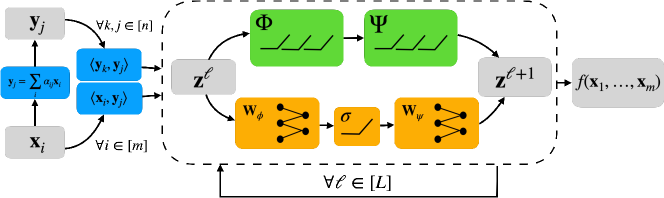
Figure 1: The geometric Kolmogorov superposition network is composed of layers that comprise two terms. The first term is based on the classical KST function representation, while the second term, similar to a residual path, is an almost linear term that helps the training of the non-linear functions.

5 Geometric Kolmogorov Superposition Networks (GKSN)

Finding the representation functions $\psi_{q},\phi_{pq}$ is still a hard non-linear optimization problem. To reduce the training complexity, we consider a representation as a layer and allow the composition of multiple layers (Figure 1). The fundamental result from Equation 5 is that we can use univariate functions on invariant features. We consider a single layer of the Geometric Kolmogorov Superposition Networks (GKSN) as the composition of the univariate functions $\phi^{\ell}_{pq}$ and the subsequent univariate functions $\psi^{\ell}_{q}$. With an abuse of notation and dropping $\ell$ dependence on the functions, we write

$$\bm{z}_{\ell+1}=\overbrace{\bm{\Psi}}^{l\times k}\circ\overbrace{\bm{\Phi}^{T}}^{k\times m}(\bm{z}_{\ell})+\overbrace{\bm{W}_{\psi}}^{l\times k^{\prime}}\sigma(\overbrace{\bm{W}_{\phi}^{T}}^{k^{\prime}\times m}\bm{z}_{\ell}),$$ (6)

or if we compute the $i$-th element,
$\displaystyle z^{\ell+1}_{i}=\underbrace{\sum_{k}\psi_{ik}\left(\sum_{j}\phi_{jk}(z^{\ell}_{j})\right)}_{\text{KST}}+\underbrace{\sum_{k}\underbrace{w_{ik}^{\psi}\sigma}_{\psi_{ik}(.)}\left(\sum_{j}\underbrace{w_{ji}^{\phi}}_{\phi_{jk}(.)}z^{\ell}_{j}\right)}_{\text{Residue term}},$ where $\circ$ is the function composition operator.

The first term is the classical KST form, while the second is inspired by the newer forms (Table 1), which contain linear terms, with a non-linear function $\sigma$ in the middle. We, therefore, assume that the original function can be represented as the sum of two functions, the first with smooth but non-linear univariate functions, the second with composition of a scaled non-linear function, and the sum of linear functions. We further assume $\sigma$ to be a fix almost everywhere smooth, continuous, and almost linear to improve the training of wide layers. The second path plays a role similar to the residual connection, which helps the training of the non-linear univariate functions.

6 Experimental Evaluation

After presenting the experimental setup, we show the performance on representative datasets in molecular dynamics such as Lennard-Jones particle system, the MD17, and MD22 datasets of the proposed architecture and compare with MLP-based approaches.

6.1 Experimental setup and baselines

We compare different models to learn invariant functions from data, from both synthetic and real datasets. In the test, we normalize the output to the interval $[0,1]$.

Symmetries

We name $O(n)$ the models with rotation and reflection symmetry, while we use $\pi$ for the models that implement permutation symmetry.

Networks

We mainly compare against the use of two layers MLP models. We implemented the KAN model of Equation 6, where we use ReLU Glorot et al. (2011) both as the basis for the KAN non-linear functions ($\psi_{q},\phi_{pq}$) and for the residual connection ($\sigma$). The name of the model contains two symbols $T$=True and $F$=False; the first boolean tells us if the node index is used as an additional $O(n)$ invariant feature. The effect of adding the index of the node is to emulate the non-permutation invariant function. The second boolean is used to show if the linear ($T$) (Equation 5) or quadratic ($F$) (Equation 4) feature is used. Therefore, $\pi~O(n)$ KAN($T,T$) is a permutation invariant model based on the KAN architecture, where node index is used as a feature, where the number of features is linear in the number of nodes $m$.

Invariant Features

While Equation 5 tells us that we can represent any invariant function with the inner products, nevertheless, to improve expressivity, we extend the invariant feature to include:

$$\|\bm{x}_{i}\|,\|\bm{y}_{j}\|,\|\bm{x}_{i}-\bm{y}_{j}\|,\langle\bm{x},\bm{y}_{j}\rangle,\sqrt{\|\bm{x}_{i}\|^{2}\|\bm{y}_{j}\|^{2}-\langle\bm{x},\bm{y}_{j}\rangle^{2}}$$

As additional invariant features, we optionally include the node index (first flag), and when present (experiments with MD17 and MD22), we also include the atom type. We have not explored alternative ways to embed the node’s additional information as input to the network. The last term is also equivalent to $\|x\times y\|$ in $n=3$ dimensions, with $\times$ the cross product.

Quadratic versus Linear features

A consequence of Equation 5, with the associated theorem, is that the number of invariant features that we need is linear with the number of nodes. We nevertheless, compare also with the quadratic version as in Equation 4.

Table 2: Huber NLL ($\uparrow$, higher is better) for the LJ dataset on different dimensions ($n\in[3,5]$) and different number of nodes $m\in[4,10,15]$. Standard deviation in parenthesis, mean computed over $3$ runs.

LJ $m/n$	$O(n)$ KAN	$O(n)$ MLP	$\pi~O(n)$ KAN	$\pi~O(n)$ MLP
4/3	8.41	8.00	7.88	7.59
	(0.19)	(0.12)	(0.15)	(0.14)
10/3	7.10	6.76	7.08	5.33
	(0.16)	(0.09)	(0.28)	(0.18)
10/5	7.15	6.71	7.23	3.72
	(0.37)	(0.28)	(0.41)	(0.60)
15/3	7.25	7.09	7.28	3.92
	(1.25)	(1.10)	(1.17)	(0.41)
15/5	6.73	6.56	6.96	1.76
	(0.18)	(0.13)	(0.24)	(1.33)

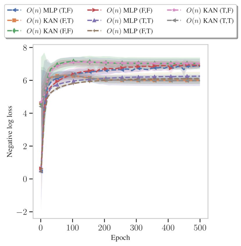
Figure 2: Test performance (Negative log Huber Loss) of $O(n)$ invariant models for the LJ experiment with $n=5$ and $m=15$. In parenthesis, the two flags indicate if the model includes the node index $(T,*)$ or not $(F,*)$; the second flag signals if the features are linear $(*,T)$ (according to Equation 5) or quadratic $(*,F)$ (according to Equation 4) in the number of nodes.

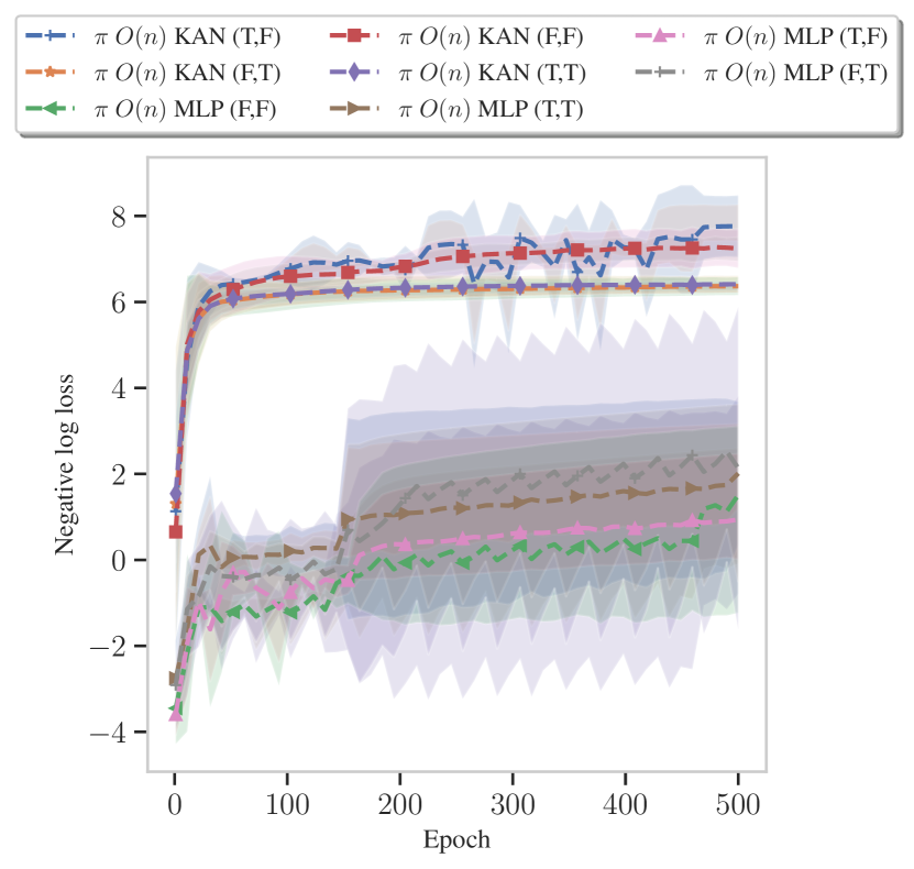
Figure 3: Test performance (Negative log Huber Loss $\uparrow$) of $O(n)$ and permutation invariant models for the LJ experiment.

6.2 Lennard-Jones experiments

Lennard-Jones potential approximates inter-molecular pair interaction and models repulsive and attractive interactions. It captures key physical principles and it is widely used to model solid, fluid, and gas states. More details are in subsection D.1. Figure 2 and Figure 3 show the test regression loss during training for a system in $3$ dimensions and with $15$ nodes. The loss is plotted in a negative log scale. We use the Huber loss, which is quadratic if the error is less than $1$, and linear if larger. The test loss for the $O(n)$ invariant model (Figure 2) is regular during training and all models seem to have similar results, while in Figure 3 the performance of permutation invariant models have quite different behavior. The MLP-based models are more unstable, while KAN-based models have a much more regular performance. Table 2 summarizes the regression accuracy at test time for all the models. The permutation invariance reduces the performances, but more remarkably on smaller systems.

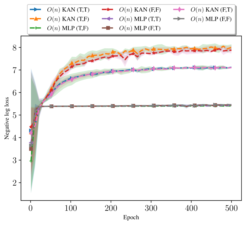
Figure 4: Test performance (Negative log Huber Loss $\uparrow$) of various models for the Ethanol dataset of MD17. $O(n)$ is the model that is invariant to rotation and reflection on $\mathbb{R}^{n}$.

Table 3: Huber NLL $\uparrow$ for the MD17 dataset (mean and standard deviation in paraenthesis)

Dataset (MD17)	$O(n)$ KAN	$O(n)$ MLP	$\pi~O(n)$ KAN	$\pi~O(n)$ MLP
Aspirin	6.44	5.62	5.69	4.73
	(0.10)	( 0.01)	(0.02)	(0.27)
Benzene	7.66	5.93	6.51	5.64
	(0.08)	(0.01)	(0.17)	( 0.13)
Ethanol	7.57	5.44	6.09	5.49
	(0.04)	(0.01)	(0.13)	(0.03)
Malonaldehyde	7.50	5.39	5.85	5.38
	(0.05 )	(0.01)	(0.04)	(0.04)
Naphthalene	6.85	5.35	5.72	4.65
	(0.07)	(0.00)	(0.09)	(0.76)
Salicylic	6.96	5.62	5.83	5.17
	(0.09)	(0.00)	(0.10)	( 0.24)
Toluene	7.05	5.68	6.03	5.40
	( 0.13)	( 0.02)	( 0.10)	( 0.11)
Uracil	7.54	5.65	6.10	5.52
	( 0.08)	(0.01)	( 0.11)	(0.05)

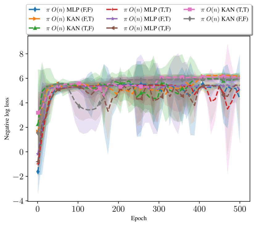
Figure 5: Test performance (Negative log Huber Loss $\uparrow$) of various models for the Ethanol dataset of MD17. $\pi-O(n)$ are the models that are invariant to rotation, reflection, and permutation.

6.3 MD17

MD17 dataset contains samples from a long molecular dynamics trajectory of a few small organic molecules Chmiela et al. (2017). For each molecule, we split into $8,000$ training and $200$ test configurations. In Table 3 we show the negative log of the Huber loss (NLL), thus the higher the value the better, aggregated over various model options, while in Table 8 we provide the test loss for each model. Figure 5 and Figure 4 show the Huber NLL at test time for the Toluene molecule for the two classes of models. The test loss in negative log scale at training for $O(n)$ invariant models in Figure 4 is stable, but reducing the number of features leads to lower performance, while KAN shows better accuracy. The training for the permutation invariant models in Figure 5 is less stable and the overall performance reduces while keeping the model size smaller. Table 3 summarizes the performance of all models in the various atomic systems of MD17, the KAN-based models show consistently better performance, even with smaller network size.

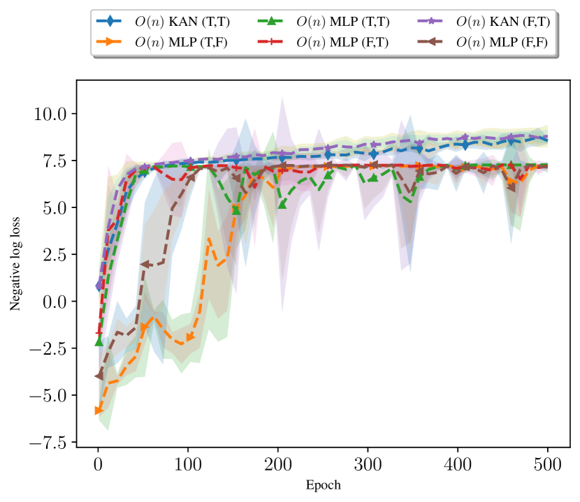
Figure 6: Test performance (Negative log Huber Loss $\uparrow$) of $O(n)$ invariant models for the Buckyball-Catcher dataset of MD22.

Table 4: Performance aggregated at the level of the model type for the MD22 dataset; the performance is the negative log of the Huber loss $\uparrow$ (mean and standard deviation in parenthesis);

Dataset (MD22)	$O(n)$ KAN	$O(n)$ MLP	$\pi~O(n)$ KAN	$\pi~O(n)$ MLP
AT-AT-CG-CG	8.02	7.61	7.73	0.82
	(0.14)	( 0.05)	( 0.05)	(0.32)
AT-AT	7.32	6.56	6.62	0.82
	( 0.21)	(0.01)	( 0.03)	(0.40)
Ac-Ala3-NHMe	5.77	5.57	5.57	1.48
	(0.07)	(0.00)	(0.01)	(1.08)
DHA	5.64	5.52	5.50	0.04
	(0.07)	( 0.00)	(0.01)	(0.82)
Buckyball-catcher	8.85	7.27	7.41	0.21
	(0.24)	(0.01)	(0.07)	(0.71)
Stachyose	6.30	5.70	5.73	1.36
	(0.12)	(0.01)	(0.03)	(1.42)

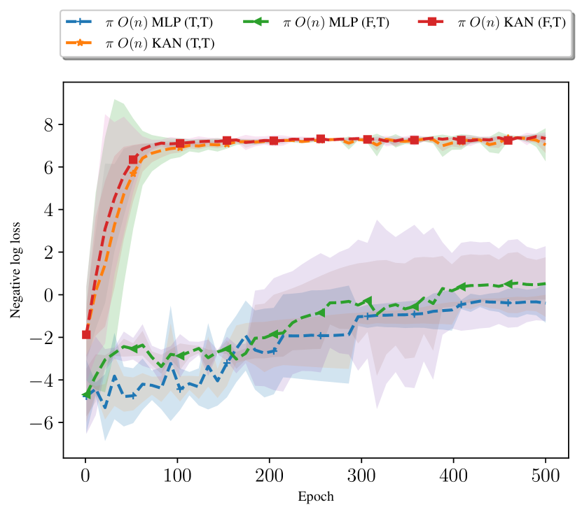
Figure 7: Training performance (Negative log Huber Loss $\uparrow$) of $O(n)$ and permutation invariant models for the Buckyball-Catcher dataset of MD22.

6.4 MD22

MD22 dataset Chmiela et al. (2023) contains samples from molecular dynamics trajectories of four major classes of biomolecules, as proteins, lipids, carbohydrates, nucleic acids, and supramolecules. In MD22, number of atoms ranges from $42$ to $370$. For each molecule, we split into $8,000$ training and $200$ test configurations. In Table 4 we show the NLL aggregated over various model options, while in Table 9 for more details information on the performance. Figure 6 and Figure 7 show the Huber NLL at test time for the Ac-Ala3-NHMe molecule, with and without permutation invariance.

Similar to the MD17 dataset, the test loss in negative log scale at training for the $O(n)$ invariant models reported in Figure 6 is stable for the KAN-based models, while MLP-based models show more unstable training and lower performances. The training for the permutation invariant models in Figure 7 is even less stable for the MLPs leading to low accuracy. Table 4 summarizes the performance of all models in the various atomic systems of MD22, the KAN-based models show consistently better performance, even with smaller network size.

7 Conclusions

We propose an extension of the KAN architecture for invariant and equivariant function representation, which is based on the theoretical results that provide us with a lower bound on the number of functions needed for approximating invariant functions. The theoretical results in section 4, provide a considerable improvement with previous results Villar et al. (2023), reducing the complexity from quadratic to linear. We further tested the performance and compared it with MLP-based architectures on an ideal physical system, the Lennard-Jones experiment, and on two real molecular datasets, the MD17 and the MD22 datasets. The performance of the proposed network architecture shows in our experiments improved performance with respect to MLP, and further investigation will show if this architecture can be extended to implement KAN-based machine learning interatomic potentials.

Supplementary Material of Geometric Kolmogorov-Arnold Superposition Theorem

Appendix A Main theorems for the Kolmogorov Superposition Theorem for invariant and equivariant functions

We first recall the Kolmogorov - Arnold and Ostrand theorems.

Theorem A.1.

Kolmogorov (1961) A function $f(x_{1},\dots,x_{m}):\mathbb{R}^{m}\to\mathbb{R}$, with $X$ a compact space, it can be represented as $f(x_{1},\dots,x_{m})=\sum_{q=1}^{2m+1}\psi_{q}(\sum_{p=1}^{m}\phi_{qp}(x_{p}))$. with $\psi_{q}:\mathbb{R}\to\mathbb{R}$ and $\phi_{qp}:[0,1]\to\mathbb{R}$ uni-variate continuous functions.

Theorem A.2.

Ostrand (1965) A function $f(x_{1},\dots,x_{m}):(X)^{m}\to\mathbb{R}$, with $X\subset\mathbb{R}^{n}$ a compact space, it can be represented as $f(x_{1},\dots,x_{m})=\sum_{q=1}^{2m+1}\psi_{q}(\sum_{p=1}^{m}\phi_{qp}(x_{p}))$. with $\bm{x}_{p}\in X^{n}$, $\phi_{qp}:X\to\mathbb{R}$ continuous functions, and $\psi_{q}:\mathbb{R}\to\mathbb{R}$ .

A.1 Permutation invariance

Lemma A.3.

(Permutation invariance) The following function is invariant to the action of permutation group:$f(x_{1},\dots,x_{m})=\sum_{q=1}^{2m+1}\psi_{q}(\sum_{p=1}^{m}\phi_{q}(x_{p}))$.

Proof.

Since the decomposition requires to the the same for a generic permutation $\pi$ then

$$\sum_{q=1}^{2m+1}\psi_{q}(\sum_{p=1}^{m}\phi_{qp}(x_{p}))=\sum_{q=1}^{2m+1}\psi_{q}(\sum_{p=1}^{m}\phi_{qp}(x_{\pi{(p)}}))$$

to be true, we need to drop the dependence of $\phi_{qp}$ on the node index $p$.

∎

Remark A.4.

We note that while the expression looks quite similar to KAT in appearance, it is not known whether the above expression is universal for arbitrary permutation invariant functions.

A.2 $O(n)$ invariance

We here consider the permutation group that acts on the input $(\bm{x}_{1},\dots,\bm{x}_{m})$ and present the architecture invariant to the action of the orthogonal group.

Theorem A.5.

($O(n)$ invariance - v1) For an $O(n)$ invariant function $f(\bm{x}_{1},\dots,\bm{x}_{m}):X^{m}\to\mathbb{R}$, with $X\subset\mathbb{R}^{n}$ a compact space, it can be represented as

$$f(\bm{x}_{1},\dots,\bm{x}_{m})=\sum_{q=1}^{2m^{2}+1}\psi_{q}(\sum_{i,j=1}^{m,m}\phi_{qij}(\langle\bm{x}_{i},\bm{x}_{j}\rangle)),$$

Proof.

Lemma 1 (First Fundamental Theorem for $O(d)$) in Villar et al. (2023) and Theorem A.1. ∎

Theorem A.6.

($O(n)$ invariance - v2) For an $O(n)$ invariant function $f(\bm{x}_{1},\dots,\bm{x}_{m}):X^{m}\to\mathbb{R}$, with $X\subset\mathbb{R}^{n}$ a compact space, it can be represented as

$$f(\bm{x}_{1},\dots,\bm{x}_{m})=\sum_{q=1}^{2mn+1}\psi_{q}\left(\sum_{i=1,j=1}^{m,n}\phi_{qij}(\langle\bm{x}_{i},\bm{y}_{j}\rangle)+\sum_{i=1,j=1}^{n,n}\phi^{\prime}_{qij}(\langle\bm{y}_{i},\bm{y}_{j}\rangle)\right),$$

where $\bm{y}_{j}^{q}=\alpha_{j}^{q}(\bm{x}_{1},\dots,\bm{x}_{m})=\sum_{p=1}^{m}\alpha_{p}^{j}\bm{x}_{p}$, with $\bm{y}_{j}^{q}$ a linear combination of $\{\bm{x}_{p}\}$ with scalars $\alpha_{p}$ such that $\text{span}(\{\bm{y}_{j}^{q}\}_{j=1}^{n})=\mathbb{R}^{n}$.

Proof.

The proof is based on the use of Lemma 1 (First Fundamental Theorem for $O(d)$) in Villar et al. (2023), Theorem A.14 and Theorem A.1. Since we define $y_{j}$ as linear combination of $x_{p}$ then also $\langle x_{p},y_{j}\rangle$ and $\langle y_{p},y_{j}\rangle$ are invariant to rotation, e.g. $\langle Rx_{p},y^{\prime}_{j}\rangle=\langle Rx_{p},\sum\alpha_{i}Rx_{i}\rangle=\langle Rx_{p},R\sum\alpha_{i}x_{i})\rangle=\langle Rx_{p},Ry_{j}\rangle=\langle x_{p},y_{j}\rangle$.

∎

Theorem A.7.

($O(n)$ invariance - v3) For an $O(n)$ invariant function $f(\bm{x}_{1},\dots,\bm{x}_{m}):X^{m}\to\mathbb{R}$, with $X\subset\mathbb{R}^{n}$ a compact space, it can be represented as

$$f(\bm{x}_{1},\dots,\bm{x}_{m})=\sum_{q=1}^{2mn+1}\psi_{q}\left(\sum_{i=1,j=1}^{m,n}\phi_{qij}(\langle\bm{x}_{i},\bm{x}_{j}\rangle)\right),$$

where we assume that $\text{span}(\{\bm{x}_{j}\}_{j=1}^{n})=\mathbb{R}^{n}$.

Proof.

Lemma 1 (First Fundamental Theorem for $O(d)$) in Villar et al. (2023), A.15 and Theorem A.1. ∎

A.3 $O(n)$ and permutation invariance

We further consider the permutation group action to the input $(\bm{x}_{1},\dots,\bm{x}_{m})$ and present the architecture invariant to the action of the permutation group.

Corollary A.8.

($O(n)$ and permutation invariance - v1) The following function is invariant to the action of the permutation group and the orthogonal group $O(n)$: $f(\bm{x}_{1},\dots,\bm{x}_{m})=\sum_{q=1}^{2mn+1}\psi_{q}\left(\sum_{i=1,j=1}^{m,m}\phi_{q}(\langle\bm{x}_{i},\bm{x}_{j}\rangle)\right)$.

Proof.

We based this result on Theorem A.5 and Lemma A.3, by removing the dependence on the node index, the function is now permutation invariant. ∎

Remark A.9.

We note that while the expression looks quite similar to KAT in appearance, it is not known whether the above expression is universal for arbitrary $O(n)$ and permutation invariant functions.

A.4 $O(n)$ equivariance

We have the corresponding equivariant version.

Theorem A.10.

($O(n)$ equivariance - v1) For an $O(n)$ equivariant function $f(x_{1},\dots,x_{m}):X^{m}\to X$, with $X\subset\mathbb{R}^{n}$ compact space, it can be represented as

$$f(\bm{x}_{1},\dots,\bm{x}_{m})=\sum_{k=1}^{m}\sum_{q=1}^{2mn+1}\psi^{k}_{q}\left(\sum_{i=1,j=1}^{m,m}\phi^{k}_{qij}(\langle\bm{x}_{i},\bm{x}_{j}\rangle)\right)\bm{x}_{k},$$

where we assume that $\text{span}(\{\bm{x}_{j}\}_{j=1}^{n})=\mathbb{R}^{n}$.

Proof.

We based this result on Theorem A.5 and on the equivariant form (Proposition 4) from Villar et al. (2023). ∎

Similar results can be obtained for the representation from Theorem A.6 or Theorem A.7.

It is possible to show that we can use the gradients of invariant functions to build a generic equivariant function, in particular, if $f(\bm{x},\dots,\bm{x}_{m})$ is invariant, then

$$\nabla_{\bm{x}_{i}}f(\bm{x},\dots,\bm{x}_{m})$$

is equivariant, as it is

$$\sum_{i=1}^{m}\alpha_{i}\nabla_{\bm{x}_{i}}f(\bm{x},\dots,\bm{x}_{m})$$

Extending the previous results with these forms is easy when $f$ is decomposed according to Theorem A.5, Theorem A.6 or Theorem A.7.

A.5 $O(n)$ equivariance and permutation invariance

We have the corresponding equivariant and permutation invariant versions.

Corollary A.11.

($O(n)$ equivariance and permutation invariance - v1) The following function is invariant to the action of the permutation group and the orthogonal group $O(n)$:

$$f(\bm{x}_{1},\dots,\bm{x}_{m})=\sum_{i=1}^{m}\sum_{q=1}^{2mn+1}\psi_{q}\left(\sum_{j=1}^{m}\phi_{q}(\langle\bm{x}_{i},\bm{x}_{j}\rangle)\right)\bm{x}_{i}.$$

Proof.

We based this result on Theorem A.10 and Lemma A.3. ∎

Remark A.12.

We note that while the expression looks quite similar to KAT in appearance, it is not known whether the above expression is universal for arbitrary $O(n)$ and permutation invariant functions.

A.6 Mapping invariant features

Lemma A.13.

Suppose that we have $\bm{X}\in\mathbb{R}^{m\times n}$ and $\bm{Y}\in\mathbb{R}^{k\times n}$ with $\rho(\bm{Y})=n,n\leq k$ then

$$\bm{X}\bm{Y}^{T}(\bm{Y}\bm{Y}^{T})^{\dagger}\bm{Y}\bm{X}^{T}=\bm{X}\bm{X}^{T},$$

where $\rho(X)$ is the matrix rank and ^† is the pseudo-inverse.

Proof.

The equality follows from these properties:

$$\bm{Y}=\bm{V}\bm{\Lambda}\bm{U},~~~\bm{V}^{T}\bm{V}=\bm{I}_{k},~~~\bm{U}^{T}\bm{U}=\bm{I}_{n}=\bm{U}\bm{U}^{T},$$

$$(\bm{Y}\bm{Y}^{T})^{\dagger}=(\bm{V}\bm{\Lambda}\bm{\Lambda}^{T}\bm{V}^{T})^{\dagger}=\bm{V}(\bm{\Lambda}\bm{\Lambda}^{T})^{\dagger}\bm{V}^{T},$$

$$\bm{Y}^{T}=\bm{U}^{T}\bm{\Lambda}^{T}\bm{V}^{T},$$

$$\bm{Y}^{T}(\bm{Y}\bm{Y}^{T})^{\dagger}\bm{Y}=\bm{U}^{T}\bm{\Lambda}^{T}\bm{V}^{T}\bm{V}(\bm{\Lambda}\bm{\Lambda}^{T})^{\dagger}\bm{V}^{T}\bm{V}\bm{\Lambda}\bm{U}=\bm{U}^{T}\bm{\Lambda}^{T}(\bm{\Lambda}\bm{\Lambda}^{T})^{\dagger}\bm{\Lambda}\bm{U}=\bm{I}_{n}.$$

∎

Theorem A.14.

(Correlation matrix representation) Given $\bm{x}_{1},\dots,\bm{x}_{m}\in\mathbb{R}^{n}$ and a set of points $\bm{y}_{1},\dots,\bm{y}_{k}\in\mathbb{R}^{n}$, such that $\rho(\bm{y}_{1},\dots,\bm{y}_{k})=n$, there is an invertible map between these two sets:

• $\{\langle\bm{x}_{i},\bm{x}_{j}\rangle\}_{i,j=1}^{m,m}$, with a total number of variable equal to $m^{2}$

• $\{\langle\bm{x}_{i},\bm{y}_{j}\rangle\}_{i,j=1}^{m,k}$, $\{\langle\bm{y}_{i},\bm{y}_{j}\rangle\}_{i,j=1}^{k,k}$ with a total number of variable equal to $mk+k^{2}$

Proof.

Define $\bm{X}=(\bm{x}_{1},\dots,\bm{x}_{m})^{T}\in\mathbb{R}^{m\times n}$ and $\bm{Y}=(\bm{y}_{1},\dots,\bm{y}_{k})^{T}\in\mathbb{R}^{k\times n}$ then

$$\bm{X}\bm{X}^{T}=\{\langle\bm{x}_{i},\bm{x}_{j}\rangle\}_{i,j=1}^{m,m},$$

$$\bm{X}\bm{Y}^{T}=\{\langle\bm{x}_{i},\bm{y}_{j}\rangle\}_{i,j=1}^{m,k},$$

and

$$\bm{Y}\bm{Y}^{T}=\{\langle\bm{y}_{i},\bm{y}_{j}\rangle\}_{i,j=1}^{k,k}.$$

We then apply A.13 to yield

$$\bm{X}\bm{X}^{T}=\bm{X}\bm{Y}^{T}(\bm{Y}\bm{Y}^{T})^{\dagger}\bm{Y}\bm{X}^{T}.$$

Notice that $\bm{Y}\bm{X}^{T}=(\bm{X}\bm{Y}^{T})^{T}$, and therefore we have the result. ∎

We define $\bm{Y}$ as a subset of $\bm{X}\in\mathbb{R}^{m\times n}$ of size $k$, then it is a matrix of dimension $k\times n$, which we ask to have rank $n$. We then can say,

Corollary A.15.

(Special case - Subset) If $\bm{Y}=\bm{X}[:n]$, with $n\leq k$, $\rho(\bm{Y})=n$, $\bm{X}\in\mathbb{R}^{m\times n}$, $m\leq k\leq n$, then there is an invertible map between these two sets:

• $\{\langle\bm{x}_{i},\bm{x}_{j}\rangle\}_{i,j=1}^{m,m}$, with a total number of variable equal to $m^{2}$

• $\{\langle\bm{x}_{i},\bm{x}_{j}\rangle\}_{i,j=1}^{m,k}$, if $\bm{y}_{j}=\bm{x}_{j}$, with a total number of variable equal to $mk$,

Proof.

We use Theorem A.14 and notice that $\bm{Y}\bm{Y}^{\operatorname{T}}$ can be derived from $\bm{Y}\bm{Y}^{\mathrm{T}}=\bm{X}[:n]\bm{X}[:n]^{\mathrm{T}}$, which are included in the previous features. ∎

A.7 Informal proof of the main theorem

There is one step in our theorem that creates concern. This step is as follows: once we change the basis for our data, we build the basis from the data itself. We now prove with a simple Python code that this is the case.

⬇

1# some help functions

2rot_gen = lambda n: np.linalg.svd(np.random.randn(n,n))[0]

3basis = lambda X: X[:n,:]

4corr = lambda X: X @ X.T

5inv = lambda X,Y: X @ Y.T

6rot = lambda X,R: X @ R

7#set the seed; it can be removed or changes

8np.random.seed(42)

9# the problem’s dimension can be changed, but m>=n

10m,n = 5,3

11# this is my data

12X = np.random.randn(m,n)

13# the correlation matrix of the data, which is an invariant feature

14C1 = corr(X)

15# we build a basis that depends on the input

16Y = basis(X)

17# compujte invariant features

18Z1 = inv(X,Y)

19# compute the correlation of the new features

20D1 = corr(Z1)

21# some rotation

22R = rot_gen(n)

23# apply the rotation to the input

24X = rot(X, R)

25# rebuild the basis

26Y = basis(X)

27# compute the invariant features

28Z2 = inv(X,Y)

29# compute the correlation with the new invariant features

30D2 = corr(Z2)

31# Question: is the correlation matrix before and after the same (we know is the same):

32print(np.linalg.norm(C1 - C2))

33# Result: 1.934545700657722e-15 (yes, numerically the same)

34# Question: is the correlation matrix with the invariant feature the same before and after (they should)

35print(np.linalg.norm(D1 - D2))

36# Result: 9.407543438562363e-15 (yes, numerically the same)

37# Question: are the invariant features the same, before and after the rotation (they better be)?

38print(np.linalg.norm(Z1 - Z2))

39# Result: 1.4220500840710913e-15 (yes, numerically the same)

Listing 1: Python based informal proof

A.8 Informal proof of A.13

⬇

1import numpy as np

2from numpy.linalg import norm

3np.random.seed(42)

4# the problem’s dimension can be changed, but m>=n

5m,n = 15,3

6k = n+2

7# create the two matrices

8X = np.random.randn(m,n)

9Y = np.random.randn(k,n)

10# Verify Theorem A.14

11print(norm(X @ Y.T @ np.linalg.pinv(Y @ Y.T) @ Y @ X.T - X@X.T))

12# Result: 1.2816111681783468e-14

Listing 2: Python based informal proof

Appendix B Complexity

The representation complexity of Equation 4 is $O(m^{4})$, which is quite larger than the complexity we have if we apply KAT directly to the coordinates of the nodes, i.e. $O(m^{2}n^{2})$, which ignores the symmetries of the problem.

However, in Equation 5, we show that we can represent the invariant function $f$ with complexity $O(m^{2}n^{2})$, thus similar to the non-invariant KAT.

Appendix C Additional Experiments

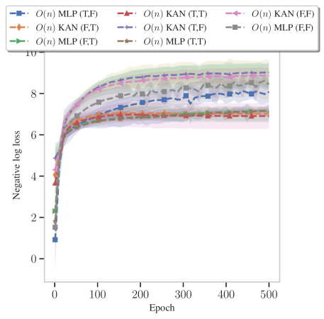
Figure 8: Test performance (Negative log Huber Loss) of various models for the linear polymers. $O(n)$ is the model that is invariant to rotation and reflection on $\mathbb{R}^{n}$, while $\pi$ is the permutation invariant model. In parenthesis, the two flags indicate if the model includes the node index and the second if the features are linear or quadratic in the number of nodes.

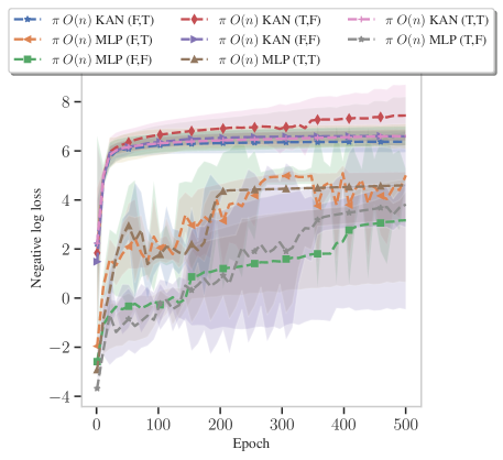
Figure 9: Test performance (Negative log Huber Loss) of various models for the linear polymers. $O(n)$ is the model that is invariant to rotation and reflection on $\mathbb{R}^{n}$, while $\pi$ is the permutation invariant model. In parenthesis, the two flags indicate if the model includes the node index and the second if the features are linear or quadratic in the number of nodes.

Table 5: Huber NLL for the Linear Polymer dataset, with $a_{i}=0$ on different dimensions ($3,5$) and different number of nodes $4,10,15$.

LinPoly-1	$O(n)$ KAN	$O(n)$ MLP	$\pi~O(n)$ KAN	$\pi~O(n)$ MLP
m4/n3	10.85	11.74	9.07	9.29
	0.52	0.18	0.40	0.33
m10/n3	8.93	9.08	7.36	6.40
	0.33	0.36	0.32	0.25
m10/n5	9.22	9.06	7.41	5.97
	0.10	0.16	0.14	0.12
m15/n3	7.99	7.98	6.91	4.82
	0.34	0.24	0.38	0.51
m15/n5	7.99	7.81	6.76	4.18
	0.33	0.16	0.39	0.78

C.1 Linear Polymer experiments

Linear polymers are chain molecules composed of repeating structural units (monomers) linked together sequentially. Linear polymers exhibit flexibility and thermoplastic behavior. Examples include polyethylene (PE), polyvinyl chloride (PVC), and polystyrene (PS), and find applications in packaging, textiles, and plastic films due to their ease of processing, recyclability, and ability to be melted and reshaped. Figure 8 and Figure 9 show the performance with $O(n)$ symmetry and with additionally permutation symmetry. Additional details in subsection D.2.

Appendix D Experiments

Table 6: Huber NLL for the LJ-2 dataset

LJ (2)	$O(n)$ KAN	$O(n)$ MLP	$\pi~O(n)$ KAN	$\pi~O(n)$ MLP
m4/n3	9.54	8.52	9.35	8.56
	0.82	0.43	0.62	0.39
m10/n3	8.66	8.22	8.49	5.73
	0.66	0.61	0.74	0.25
m10/n5	7.52	7.02	7.19	4.84
	0.27	0.10	0.32	0.19
m15/n3	9.45	9.35	9.89	3.91
	1.32	1.43	2.11	0.79
m15/n5	6.66	6.47	6.74	2.36
	0.23	0.27	0.25	1.33

D.1 Lennard-Jonnes

For the Lennard-Jonnes (LJ) experiments, we generate $m$ particles in $n$ dimensional space. The interaction between particles is described by the LJ potential,

$$U_{\text{LJ}}(r)=f((a/r)^{12}-(a/r)^{6})$$

where $r$ is the distance between two particles and $a$ is a parameter that defines the minimum energy of the interaction, while $f(x)=x+\sum_{l=1}^{3}a_{l}\sin(w_{l}x)$, with $a_{1}=1,a_{2}=.3,a_{3}=.1,w_{1}=11,w_{2}=30,w_{3}=50$ (or $a_{1}=a_{2}=a_{3}=0$), is an oscillatory term. After generating the particles, we perform an energy minimization step to relax the system towards a lower energy state, avoiding large energy contributions caused by the random initialization of the particle positions.

D.2 Linear polymers

As an additional experiment, we consider linear polymers of size $m$. The particles are connected to the previous and the following particle by a bond. The interaction between the bond depends quadratically on the difference between the current distance and the desired distance,

$$U_{\text{bond}}(r)=f(\|d-\hat{d}\|^{2})+U_{\text{LJ}}(r)$$

and $f(x)=x+\sum_{l=1}^{3}a_{l}\sin(w_{l}x)$ is an oscillatory term. For the unbonded particle, the LJ potential is used, as before.

Table 7: Huber NLL for the LinPoly-2 dataset

LinPoly-2	$O(n)$ KAN	$O(n)$ MLP	$\pi~O(n)$ KAN	$\pi~O(n)$ MLP
m4/n3	10.51	8.78	8.41	7.13
	0.17	0.13	0.27	0.08
m10/n3	8.30	7.50	7.26	4.73
	0.40	0.18	0.39	0.78
m10/n5	8.36	7.77	7.18	4.11
	0.45	0.16	0.48	0.64
m15/n3	7.40	7.47	6.95	2.98
	0.42	0.32	0.48	0.99
m15/n5	7.45	7.54	6.94	2.54
	0.45	0.17	0.56	1.00

D.3 MD17

Table 8 shows in detail the performance of the different models on the MD17 dataset.

Table 8: Huber NLL for the MD17 dataset

Dataset (MD17)	aspirin		benzene2017		ethanol		malonaldehyde		naphthalene		salicylic		toluene		uracil
$O(n)$ KAN (F,F)	6.77	0.16	8.02	0.09	7.94	0.04	7.84	0.03	7.42	0.04	7.54	0.14	7.60	0.21	8.03	0.13
$O(n)$ KAN (F,T)	6.08	0.01	7.29	0.03	7.14	0.03	7.12	0.04	6.29	0.08	6.41	0.03	6.50	0.06	7.08	0.00
$O(n)$ KAN (T,F)	6.83	0.20	8.06	0.15	8.06	0.04	7.90	0.07	7.39	0.14	7.53	0.13	7.54	0.18	8.04	0.11
$O(n)$ KAN (T,T)	6.09	0.04	7.27	0.06	7.13	0.03	7.16	0.07	6.30	0.03	6.36	0.05	6.54	0.06	7.01	0.09
$O(n)$ MLP (F,F)	5.63	0.00	5.98	0.02	5.47	0.01	5.40	0.01	5.37	0.00	5.65	0.00	5.69	0.02	5.70	0.01
$O(n)$ MLP (F,T)	5.63	0.01	5.91	0.00	5.46	0.03	5.42	0.02	5.34	0.00	5.62	0.01	5.71	0.00	5.61	0.00
$O(n)$ MLP (T,F)	5.61	0.01	5.93	0.02	5.41	0.01	5.37	0.01	5.36	0.01	5.61	0.00	5.64	0.04	5.69	0.01
$O(n)$ MLP (T,T)	5.61	0.00	5.90	0.00	5.43	0.01	5.38	0.01	5.33	0.00	5.61	0.01	5.68	0.01	5.61	0.00
$\pi~O(n)$ KAN (F,F)	5.68	0.02	6.73	0.18	5.95	0.18	5.83	0.04	5.82	0.10	5.81	0.14	6.11	0.11	6.21	0.11
$\pi~O(n)$ KAN (F,T)	5.69	0.02	6.27	0.10	6.24	0.13	5.91	0.01	5.65	0.06	5.82	0.00	5.96	0.12	5.94	0.14
$\pi~O(n)$ KAN (T,F)	5.69	0.02	6.69	0.19	6.01	0.07	5.80	0.03	5.84	0.10	5.90	0.16	6.06	0.11	6.32	0.05
$\pi~O(n)$ KAN (T,T)	5.69	0.02	6.34	0.20	6.15	0.16	5.87	0.07	5.59	0.11	5.80	0.10	5.98	0.05	5.93	0.16
$\pi~O(n)$ MLP (F,F)	4.28	0.39	5.73	0.10	5.55	0.08	5.41	0.05	5.07	0.16	5.27	0.03	5.41	0.06	5.58	0.07
$\pi~O(n)$ MLP (F,T)	5.45	0.05	5.77	0.05	5.49	0.01	5.40	0.03	5.29	0.02	5.53	0.06	5.64	0.04	5.58	0.02
$\pi~O(n)$ MLP (T,F)	3.84	0.59	5.47	0.26	5.44	0.01	5.34	0.04	3.08	2.83	4.41	0.82	5.07	0.27	5.47	0.03
$\pi~O(n)$ MLP (T,T)	5.34	0.06	5.58	0.11	5.46	0.01	5.37	0.03	5.17	0.03	5.48	0.07	5.49	0.05	5.45	0.08

D.4 MD22

Table 9 shows in detail the performance of the different models on the MD22 dataset.

Table 9: Huber NLL for the MD22 dataset

Dataset (MD22)	AT-AT-CG-CG		AT-AT		Ac-Ala3-NHMe		DHA		buckyball-catcher		stachyose
$O(n)$ KAN (F,F)	NaN	NaN	7.42	0.30	5.95	0.07	5.71	0.10	NaN	NaN	NaN	NaN
$O(n)$ KAN (F,T)	7.94	0.19	7.27	0.18	5.65	0.03	5.59	0.01	8.92	0.20	6.24	0.11
$O(n)$ KAN (T,F)	NaN	NaN	7.20	0.33	5.85	0.13	5.67	0.14	NaN	NaN	NaN	NaN
$O(n)$ KAN (T,T)	8.10	0.09	7.38	0.05	5.64	0.04	5.56	0.01	8.77	0.28	6.36	0.13
$O(n)$ MLP (F,F)	7.66	0.07	6.57	0.01	5.58	0.00	5.53	0.00	7.30	0.00	5.74	0.00
$O(n)$ MLP (F,T)	7.64	0.03	6.57	0.01	5.58	0.00	5.51	0.00	7.27	0.00	5.70	0.01
$O(n)$ MLP (T,F)	7.57	0.04	6.56	0.01	5.57	0.01	5.53	0.00	7.25	0.02	5.70	0.02
$O(n)$ MLP (T,T)	7.59	0.05	6.55	0.03	5.56	0.00	5.51	0.00	7.27	0.01	5.67	0.00
$\pi~O(n)$ KAN (F,F)	NaN	NaN	6.60	0.02	5.58	0.01	5.49	0.00	NaN	NaN	NaN	NaN
$\pi~O(n)$ KAN (F,T)	7.71	0.04	6.61	0.07	5.56	0.00	5.51	0.01	7.43	0.08	5.70	0.02
$\pi~O(n)$ KAN (T,F)	7.75	NaN	6.61	0.02	5.57	0.00	5.50	0.01	NaN	NaN	5.77	NaN
$\pi~O(n)$ KAN (T,T)	7.74	0.07	6.64	0.03	5.56	0.01	5.52	0.01	7.39	0.06	5.73	0.03
$\pi~O(n)$ MLP (F,F)	NaN	NaN	NaN	NaN	-0.04	1.53	-0.59	0.11	NaN	NaN	NaN	NaN
$\pi~O(n)$ MLP (F,T)	1.25	0.36	2.10	0.36	3.76	0.20	2.09	0.35	0.61	1.21	1.27	1.82
$\pi~O(n)$ MLP (T,F)	NaN	NaN	-1.29	0.22	0.23	0.26	-2.68	1.40	NaN	NaN	NaN	NaN
$\pi~O(n)$ MLP (T,T)	0.39	0.28	1.64	0.62	1.99	2.35	1.35	1.43	-0.18	0.20	1.46	1.01

Appendix E Model parameters

Parameter	Value	Comment
Number of epochs	500	We use 500 for the MD17 and MD22, while 1000 for the LJ experiments
batch size	4092
loss	Huber	We selected Huber, compared to MSE, since it enables better training
em lr	0.01,	learning rate for energy minimization for LJ experiments
em niters	500	number of steps for energy minimization for LJ experiments
learning rate	0.001	we experimented with multiple rate and fix this for all experiments
num samples	10000	We fix the number of samples, if the dataset contains more data, we first permute the data (same for all experiments) and select the first 10000 samples.
trsamples	8000	we split 80/20 training and testing
optimizer	AdamW
weight decay	$1e-9$	Weight decay is used to stabilize the training
scheduler	ReduceLROnPlateau	The scheduler helps with different system requirement
KAN layers	[input dim, 16, 16, 1]	the architecture size has been selected in the hyper-parameter search
KAN orders	[8,8,8]	This is the number of basis per function
KAN Basis	ReLU	While KAN networks use Spline as basis, we experimented with ReLU, GeLU, Sigmoid, and Chebichev Polynomial, ReLU provided the most reliable solution
MLP layers	[input dim, 128, 128, 1]	the architecture size has been selected in the hyper-parameter search

Table 10: Hyper-parameters used during training

E.1 Hyper-parameters and Hyper-parameter search

Table 10 show the hyper-parameters used during training for the MLP and KAN-based architectures. We implemented a separate hyper-parameter search on both MLP and KAN architecture based on the synthetic dataset, we tested the different sizes of architecture: small (128/16), medium (256/32), and large (512/64); and selected the small for both systems.

While KAN networks use Spline as the basis, we experimented with ReLU, GeLU, Sigmoid, and Chebichev Polynomial, ReLU provided the most reliable solution across test cases.

E.2 LJ

Table 11 shows the number of parameters per model for the LJ experiments with $m=4$ and $n=3$. The impact of the presentation is already visible. KAN is always smaller. Table 12 and Table 13 show the network size for $m=15$ and $n=3,5$. As the input increases the KAN has more parameters than the equivalent MLP.

Table 11: Network sizes during the $4/3$ experiments

system	model	options	size
m4/n3	$O(n)$ KAN	FF	9911
m4/n3	$O(n)$ KAN	FT	9911
m4/n3	$O(n)$ KAN	TF	12044
m4/n3	$O(n)$ KAN	TT	12044
m4/n3	$O(n)$ MLP	FF	22145
m4/n3	$O(n)$ MLP	FT	22145
m4/n3	$O(n)$ MLP	TF	23681
m4/n3	$O(n)$ MLP	TT	23681
m4/n3	$\pi O(n)$ KAN	FF	4167
m4/n3	$\pi O(n)$ KAN	FT	4167
m4/n3	$\pi O(n)$ KAN	TF	4475
m4/n3	$\pi O(n)$ KAN	TT	4475
m4/n3	$\pi O(n)$ MLP	FF	17665
m4/n3	$\pi O(n)$ MLP	FT	17665
m4/n3	$\pi O(n)$ MLP	TF	17921
m4/n3	$\pi O(n)$ MLP	TT	17921

Table 12: Network sizes during the $15/3$ experiments

system	model	options	size
m15/n3	$O(n)$ KAN	FF	250887
m15/n3	$O(n)$ KAN	FT	63691
m15/n3	$O(n)$ KAN	TF	371803
m15/n3	$O(n)$ KAN	TT	87687
m15/n3	$O(n)$ MLP	FF	110849
m15/n3	$O(n)$ MLP	FT	51713
m15/n3	$O(n)$ MLP	TF	137729
m15/n3	$O(n)$ MLP	TT	61697
m15/n3	$\pi O(n)$ KAN	FF	4167
m15/n3	$\pi O(n)$ KAN	FT	4167
m15/n3	$\pi O(n)$ KAN	TF	4475
m15/n3	$\pi O(n)$ KAN	TT	4475
m15/n3	$\pi O(n)$ MLP	FF	17665
m15/n3	$\pi O(n)$ MLP	FT	17665
m15/n3	$\pi O(n)$ MLP	TF	17921
m15/n3	$\pi O(n)$ MLP	TT	17921

Table 13: Network sizes during the $15/5$ experiments

system	model	options	size
m15/n5	$O(n)$ KAN	FF	250887
m15/n5	$O(n)$ KAN	FT	111906
m15/n5	$O(n)$ KAN	TF	371803
m15/n5	$O(n)$ KAN	TT	159216
m15/n5	$O(n)$ MLP	FF	110849
m15/n5	$O(n)$ MLP	FT	70529
m15/n5	$O(n)$ MLP	TF	137729
m15/n5	$O(n)$ MLP	TT	85889
m15/n5	$\pi O(n)$ KAN	FF	4167
m15/n5	$\pi O(n)$ KAN	FT	4167
m15/n5	$\pi O(n)$ KAN	TF	4475
m15/n5	$\pi O(n)$ KAN	TT	4475
m15/n5	$\pi O(n)$ MLP	FF	17665
m15/n5	$\pi O(n)$ MLP	FT	17665
m15/n5	$\pi O(n)$ MLP	TF	17921
m15/n5	$\pi O(n)$ MLP	TT	17921

E.3 MD17

Table 14 shows the number of parameters for the models used in the experiments. The permutation invariant version reduces the need for parameters considerably.

Table 14: Network sizes during the aspirin experiments

dataset	model	options	size
aspirin	$O(n)$ KAN	FF	1186625
aspirin	$O(n)$ KAN	FT	147811
aspirin	$O(n)$ KAN	TF	1692200
aspirin	$O(n)$ KAN	TT	197535
aspirin	$O(n)$ MLP	FF	258689
aspirin	$O(n)$ MLP	FT	82433
aspirin	$O(n)$ MLP	TF	312449
aspirin	$O(n)$ MLP	TT	97025
aspirin	$\pi O(n)$ KAN	FF	4475
aspirin	$\pi O(n)$ KAN	FT	4475
aspirin	$\pi O(n)$ KAN	TF	4783
aspirin	$\pi O(n)$ KAN	TT	4783
aspirin	$\pi O(n)$ MLP	FF	17921
aspirin	$\pi O(n)$ MLP	FT	17921
aspirin	$\pi O(n)$ MLP	TF	18177
aspirin	$\pi O(n)$ MLP	TT	18177

E.4 MD22

As for the MD17 dataset, also for MD22, Table 15 shows the number of parameters for the models used in the experiments. The permutation invariant version reduces the need for parameters considerably.

Table 15: Network sizes during the AT-AT-CG-CG experiments

dataset	model	options	size
AT-AT-CG-CG	$O(n)$ KAN	FF	974480535
AT-AT-CG-CG	$O(n)$ KAN	FT	2938488
AT-AT-CG-CG	$O(n)$ KAN	TF	1453151821
AT-AT-CG-CG	$O(n)$ KAN	TT	4256886
AT-AT-CG-CG	$O(n)$ MLP	FF	7969025
AT-AT-CG-CG	$O(n)$ MLP	FT	417665
AT-AT-CG-CG	$O(n)$ MLP	TF	9736193
AT-AT-CG-CG	$O(n)$ MLP	TT	506753
AT-AT-CG-CG	$\pi O(n)$ KAN	FT	4475
AT-AT-CG-CG	$\pi O(n)$ KAN	TF	4783
AT-AT-CG-CG	$\pi O(n)$ KAN	TT	4783
AT-AT-CG-CG	$\pi O(n)$ MLP	FF	17921
AT-AT-CG-CG	$\pi O(n)$ MLP	FT	17921
AT-AT-CG-CG	$\pi O(n)$ MLP	TF	18177
AT-AT-CG-CG	$\pi O(n)$ MLP	TT	18177

References

- Abueidda et al. (2024) Abueidda, D. W., Pantidis, P., and Mobasher, M. E. Deepokan: Deep operator network based on kolmogorov arnold networks for mechanics problems, 2024. URL https://arxiv.org/abs/2405.19143.
- Aghaei (2024) Aghaei, A. A. rkan: Rational kolmogorov-arnold networks, 2024. URL https://arxiv.org/abs/2406.14495.
- Arnold (1959) Arnold, V. I. On functions of three variables. Doklady Akademii Nauk SSSR, 114:679–681, 1959.
- Batatia et al. (2023) Batatia, I., Kovács, D. P., Simm, G. N. C., Ortner, C., and Csányi, G. Mace: Higher order equivariant message passing neural networks for fast and accurate force fields. (arXiv:2206.07697), January 2023. doi: 10.48550/arXiv.2206.07697. URL http://arxiv.org/abs/2206.07697. arXiv:2206.07697 [stat].
- Batzner et al. (2022) Batzner, S., Musaelian, A., Sun, L., Geiger, M., Mailoa, J. P., Kornbluth, M., Molinari, N., Smidt, T. E., and Kozinsky, B. E(3)-Equivariant Graph Neural Networks for Data-Efficient and Accurate Interatomic Potentials. Nature Communications, 13(1):2453, May 2022. ISSN 2041-1723. doi: 10.1038/s41467-022-29939-5.
- Bozorgasl & Chen (2024) Bozorgasl, Z. and Chen, H. Wav-kan: Wavelet kolmogorov-arnold networks, 2024. URL https://arxiv.org/abs/2405.12832.
- Braun (2009) Braun, J. An Application of Kolmogorov’s Superposition Theorem to Function Reconstruction in Higher Dimensions. PhD thesis, Universitäts-und Landesbibliothek Bonn, 2009.
- Braun & Griebel (2009) Braun, J. and Griebel, M. On a constructive proof of Kolmogorov’s superposition theorem. Constructive approximation, 30:653–675, 2009.
- Carlo et al. (2024) Carlo, G. D., Mastropietro, A., and Anagnostopoulos, A. Kolmogorov-arnold graph neural networks, 2024. URL https://arxiv.org/abs/2406.18354.
- Chmiela et al. (2017) Chmiela, S., Tkatchenko, A., Sauceda, H. E., Poltavsky, I., Schütt, K. T., and Müller, K.-R. Machine learning of accurate energy-conserving molecular force fields. Science advances, 3(5):e1603015, 2017.
- Chmiela et al. (2023) Chmiela, S., Vassilev-Galindo, V., Unke, O. T., Kabylda, A., Sauceda, H. E., Tkatchenko, A., and Müller, K.-R. Accurate global machine learning force fields for molecules with hundreds of atoms. Science Advances, 9(2):eadf0873, 2023.
- Ferdaus et al. (2024) Ferdaus, M. M., Abdelguerfi, M., Ioup, E., Dobson, D., Niles, K. N., Pathak, K., and Sloan, S. KANICE: Kolmogorov-Arnold Networks with Interactive Convolutional Elements, October 2024.
- Finzi et al. (2021) Finzi, M., Welling, M., and Wilson, A. G. A practical method for constructing equivariant multilayer perceptrons for arbitrary matrix groups. CoRR, abs/2104.09459, 2021. URL https://arxiv.org/abs/2104.09459.
- Frank et al. (2024) Frank, J. T., Unke, O. T., Müller, K.-R., and Chmiela, S. A euclidean transformer for fast and stable machine learned force fields. Nature Communications, 15(1):6539, August 2024. ISSN 2041-1723. doi: 10.1038/s41467-024-50620-6.
- Galitsky (2024) Galitsky, B. A. Kolmogorov-arnold network for word-level explainable meaning representation. Preprints, 2024. URL https://www.preprints.org/manuscript/202405.1981. Retrieved from https://www.preprints.org/manuscript/202405.1981.
- Gasteiger et al. (2022) Gasteiger, J., Groß, J., and Günnemann, S. Directional message passing for molecular graphs. (arXiv:2003.03123), April 2022. doi: 10.48550/arXiv.2003.03123. URL http://arxiv.org/abs/2003.03123. arXiv:2003.03123 [cs].
- Girosi & Poggio (1989) Girosi, F. and Poggio, T. Representation properties of networks: Kolmogorov’s theorem is irrelevant. Neural Computation, 1(4):465–469, 1989.
- Glorot et al. (2011) Glorot, X., Bordes, A., and Bengio, Y. Deep sparse rectifier neural networks. In Proceedings of the fourteenth international conference on artificial intelligence and statistics, pp. 315–323. JMLR Workshop and Conference Proceedings, 2011.
- Goodman & Wallach (2009) Goodman, R. and Wallach, N. R. Symmetry, representations, and invariants, volume 255. Springer, 2009.
- Guilhoto & Perdikaris (2024) Guilhoto, L. F. and Perdikaris, P. Deep learning alternatives of the kolmogorov superposition theorem. (arXiv:2410.01990), October 2024. doi: 10.48550/arXiv.2410.01990. URL http://arxiv.org/abs/2410.01990. arXiv:2410.01990.
- Hecht-Nielsen (1987) Hecht-Nielsen, R. Kolmogorov’s mapping neural network existence theorem. In Proceedings of the international conference on Neural Networks, volume 3, pp. 11–14. IEEE press New York, NY, USA, 1987.
- Hornik et al. (1989) Hornik, K., Stinchcombe, M., and White, H. Multilayer feedforward networks are universal approximators. Neural networks, 2(5):359–366, 1989.
- Hu et al. (2024) Hu, L., Wang, Y., and Lin, Z. EKAN: Equivariant Kolmogorov-Arnold Networks, October 2024.
- Igelnik & Parikh (2003) Igelnik, B. and Parikh, N. Kolmogorov’s spline network. IEEE transactions on neural networks, 14(4):725–733, 2003.
- Inzirillo & Genet (2024) Inzirillo, H. and Genet, R. Sigkan: Signature-weighted kolmogorov-arnold networks for time series, 2024. URL https://arxiv.org/abs/2406.17890.
- Ji et al. (2024) Ji, T., Hou, Y., and Zhang, D. A comprehensive survey on kolmogorov arnold networks (kan). (arXiv:2407.11075), December 2024. doi: 10.48550/arXiv.2407.11075. URL http://arxiv.org/abs/2407.11075. arXiv:2407.11075 [cs].
- Krková (1991) Krková, V. Kolmogorov’s theorem is relevant. Neural Computation, 3(4):617–622, 1991.
- Kolmogorov (1957) Kolmogorov, A. N. On the representation of continuous functions of many variables by superposition of continuous functions of one variable and addition. In Doklady Akademii Nauk, volume 114, pp. 953–956. Russian Academy of Sciences, 1957.
- Kolmogorov (1961) Kolmogorov, A. N. On the representation of continuous functions of several variables by superpositions of continuous functions of a smaller number of variables. American Mathematical Society, 1961.
- Köppen (2002) Köppen, M. On the training of a kolmogorov network. In Artificial Neural Networks—ICANN 2002: International Conference Madrid, Spain, August 28–30, 2002 Proceedings 12, pp. 474–479. Springer, 2002.
- Kreinovich et al. (1996) Kreinovich, V., Nguyen, H. T., and Sprecher, D. A. Normal Forms For Fuzzy Logic — An Application Of Kolmogorov’S Theorem. International Journal of Uncertainty, Fuzziness and Knowledge-Based Systems, 04(04):331–349, August 1996. ISSN 0218-4885, 1793-6411. doi: 10.1142/S0218488596000196.
- Kŭrková (1992) Kŭrková, V. Kolmogorov’s theorem and multilayer neural networks. Neural networks, 5(3):501–506, 1992.
- Kůrková (1991) Kůrková, V. Kolmogorov’s theorem and multilayer neural networks. Neural Networks, 5(3):501–506, 1991.
- Laczkovich (2021) Laczkovich, M. A superposition theorem of Kolmogorov type for bounded continuous functions. Journal of Approximation Theory, 269:105609, 2021.
- Lai & Shen (2021) Lai, M.-J. and Shen, Z. The kolmogorov superposition theorem can break the curse of dimensionality when approximating high dimensional functions. arXiv preprint arXiv:2112.09963, 2021.
- Liao & Smidt (2023) Liao, Y.-L. and Smidt, T. Equiformer: Equivariant graph attention transformer for 3d atomistic graphs. (arXiv:2206.11990), February 2023. doi: 10.48550/arXiv.2206.11990. URL http://arxiv.org/abs/2206.11990. arXiv:2206.11990 [cs].
- Liu et al. (2024a) Liu, Z., Wang, Y., Vaidya, S., Ruehle, F., Halverson, J., Soljačić, M., Hou, T. Y., and Tegmark, M. Kan: Kolmogorov-arnold networks. (arXiv:2404.19756), June 2024a. doi: 10.48550/arXiv.2404.19756. URL http://arxiv.org/abs/2404.19756. arXiv:2404.19756 [cs].
- Liu et al. (2024b) Liu, Z., Wang, Y., Vaidya, S., Ruehle, F., Halverson, J., Soljačić, M., Hou, T. Y., and Tegmark, M. Kan: Kolmogorov-arnold networks, 2024b.
- Lorentz (1976) Lorentz, G. G. Approximation of Functions. Chelsea Publishing Company, 1976.
- Mostajeran & Faroughi (2024) Mostajeran, F. and Faroughi, S. A. Epi-ckans: Elasto-plasticity informed kolmogorov-arnold networks using chebyshev polynomials, 2024. URL https://arxiv.org/abs/2410.10897.
- Noether (1971) Noether, E. Invariant variation problems. Transport Theory and Statistical Physics, 1(3):186–207, 1971.
- Ostrand (1965) Ostrand, P. A. Dimension of Metric Spaces and Hilbert’S Problem 13. 1965.
- Poggio (2022) Poggio, T. How deep sparse networks avoid the curse of dimensionality: Efficiently computable functions are compositionally sparse. CBMM Memo, 10:2022, 2022.
- Ruhe et al. (2023) Ruhe, D., Brandstetter, J., and Forré, P. Clifford Group Equivariant Neural Networks, October 2023.
- Satorras et al. (2022) Satorras, V. G., Hoogeboom, E., and Welling, M. E(n) equivariant graph neural networks. (arXiv:2102.09844), February 2022. doi: 10.48550/arXiv.2102.09844. URL http://arxiv.org/abs/2102.09844. arXiv:2102.09844 [cs].
- Schütt et al. (2017) Schütt, K. T., Kindermans, P.-J., Sauceda, H. E., Chmiela, S., Tkatchenko, A., and Müller, K.-R. SchNet: A continuous-filter convolutional neural network for modeling quantum interactions. (arXiv:1706.08566), December 2017. doi: 10.48550/arXiv.1706.08566.
- Seydi et al. (2024) Seydi, M. et al. Enhancing hyperspectral image classification with wavelet-based kolmogorov-arnold networks. IEEE Geoscience and Remote Sensing Letters, 21(4):300–315, 2024.
- Shuai & Li (2024) Shuai, H. and Li, F. Physics-informed kolmogorov-arnold networks for power system dynamics, 2024. URL https://arxiv.org/abs/2408.06650.
- Shukla et al. (2024) Shukla, K., Toscano, J. D., Wang, Z., Zou, Z., and Karniadakis, G. E. A comprehensive and fair comparison between mlp and kan representations for differential equations and operator networks, 2024. URL https://arxiv.org/abs/2406.02917.
- Somvanshi et al. (2024) Somvanshi, S., Javed, S. A., Islam, M. M., Pandit, D., and Das, S. A Survey on Kolmogorov-Arnold Network, November 2024.
- Sprecher (1963) Sprecher, D. Ph.D. Dissertation. PhD thesis, University of Maryland, 1963.
- Sprecher (1965) Sprecher, D. A. On the structure of continuous functions of several variables. Transactions of the American Mathematical Society, 115:340–355, 1965.
- Sprecher (1996) Sprecher, D. A. A numerical implementation of Kolmogorov’s superpositions. Neural Networks, 9(5):765–772, 1996.
- SS et al. (2024) SS, S., AR, K., R, G., and KP, A. Chebyshev polynomial-based kolmogorov-arnold networks: An efficient architecture for nonlinear function approximation, 2024. URL https://arxiv.org/abs/2405.07200.
- Thomas et al. (2018a) Thomas, N., Smidt, T., Kearnes, S., Yang, L., Li, L., Kohlhoff, K., and Riley, P. Tensor field networks: Rotation- and translation-equivariant neural networks for 3d point clouds. (arXiv:1802.08219), May 2018a. doi: 10.48550/arXiv.1802.08219. URL http://arxiv.org/abs/1802.08219. arXiv:1802.08219 [cs].
- Thomas et al. (2018b) Thomas, N., Smidt, T., Kearnes, S., Yang, L., Li, L., Kohlhoff, K., and Riley, P. Tensor field networks: Rotation- and translation-equivariant neural networks for 3D point clouds, May 2018b.
- Unke et al. (2021) Unke, O. T., Chmiela, S., Sauceda, H. E., Gastegger, M., Poltavsky, I., Schütt, K. T., Tkatchenko, A., and Müller, K.-R. Machine learning force fields. Chemical Reviews, 121(16):10142–10186, August 2021. ISSN 0009-2665, 1520-6890. doi: 10.1021/acs.chemrev.0c01111. arXiv:2010.07067 [physics].
- Villar et al. (2023) Villar, S., Hogg, D. W., Storey-Fisher, K., Yao, W., and Blum-Smith, B. Scalars are universal: Equivariant machine learning, structured like classical physics, February 2023.
- Wang et al. (2024) Wang, Y., Sun, J., Bai, J., Anitescu, C., Eshaghi, M. S., Zhuang, X., Rabczuk, T., and Liu, Y. Kolmogorov arnold informed neural network: A physics-informed deep learning framework for solving forward and inverse problems based on kolmogorov arnold networks, 2024. URL https://arxiv.org/abs/2406.11045.
- Xu et al. (2024a) Xu, J., Chen, Z., Li, J., Yang, S., Wang, W., Hu, X., and Ngai, E. C. H. Fourierkan-gcf: Fourier kolmogorov-arnold network – an effective and efficient feature transformation for graph collaborative filtering, 2024a. URL https://arxiv.org/abs/2406.01034.
- Xu et al. (2024b) Xu, K., Chen, L., and Wang, S. Are kan effective for identifying and tracking concept drift in time series?, 2024b. URL https://arxiv.org/abs/2410.10041.
- Xu et al. (2024c) Xu, K., Chen, L., and Wang, S. Kolmogorov-arnold networks for time series: Bridging predictive power and interpretability, 2024c. URL https://arxiv.org/abs/2406.02496.
- Yang & Wang (2024) Yang, X. and Wang, X. Kolmogorov-Arnold Transformer, September 2024.
- Zaverkin et al. (2024) Zaverkin, V., Alesiani, F., Maruyama, T., Errica, F., Christiansen, H., Takamoto, M., Weber, N., and Niepert, M. Higher-rank irreducible cartesian tensors for equivariant message passing. (arXiv:2405.14253), November 2024. doi: 10.48550/arXiv.2405.14253. URL http://arxiv.org/abs/2405.14253. arXiv:2405.14253 [cs].