Arecibo Multi-frequency IPS Observations: Solar Wind Density Turbulence Scale Sizes and their Anisotropy

1 Introduction

The remote-sensing technique of ‘interplanetary scintillation’ (IPS) is a powerful tool for probing the solar wind over a wide range of heliocentric distances, from near the Sun out to the Earth’s orbit, and both within and away from the ecliptic plane – regions often inaccessible to space missions (e.g., Hewish, Scott, and Wills 1964; Coles 1978; Kojima and Kakinuma 1987; Manoharan and Ananthakrishnan 1990; Manoharan 1993; Shishov et al. 2010). IPS also offers a simple method to identify compact sub-arcsecond structures in radio sources (e.g., Little and Hewish 1966; Salpeter 1967; Rao, Bhandari, and Ananthakrishnan 1974; Readhead, Kemp, and Hewish 1978; Manoharan 2009; Morgan et al. 2019). Routine IPS observations at 327 MHz have been conducted over three solar cycles using the multi-antenna system at the Institute for Space-Earth Environmental Research, Nagoya University (Kojima and Kakinuma 1990; Tokumaru, Kojima, and Fujiki 2012), and the large-steerable Ooty Radio Telescope at the Radio Astronomy Centre of the National Centre for Radio Astrophysics, Tata Institute of Fundamental Research (Swarup et al. 1971; Manoharan 1993; Manoharan 2012). The Mexican Array Radio Telescope (MEXART) operates as a dedicated transit IPS telescope at a central frequency of 140 MHz (Gonzalez-Esparza et al. 2022), while the Big Scanning Array of the Lebedev Physical Institute regularly monitors IPS at 111 MHz (Chashei et al. 2023). These systems, operating within the frequency range of approximately $\sim$110 – 327 MHz, constitute the Worldwide IPS Stations (WIPSS) network (Bisi et al. 2021), which aims to provide standardized IPS data for tomographic reconstruction of the solar wind (e.g., Manoharan 2010; Jackson et al. 2020) to support and improve space-weather science and forecasting capabilities.

Recently, astronomical facilities operating between 50 and 250 MHz, such as the Low Frequency Array (LOFAR) (Fallows et al. 2013) and the Murchison Widefield Array (MWA) at the Murchison Radio Observatory (Kaplan et al. 2015), have also been employed for IPS-science-based studies. Additionally, IPS observations with the MWA telescope have been extensively used to identify and survey compact components in radio sources (Chhetri et al. 2018).

Numerous IPS studies conducted with various radio telescopes at different frequencies have provided significant insights into the large-scale structure and long-term variations of the solar wind, offering valuable contributions to solar physics, particularly in understanding inner heliospheric processes and space weather phenomena such as coronal mass ejections (CMEs), solar wind interaction regions, and intense interplanetary shock waves that can cause severe geomagnetic storms and disrupt critical ground- and space-based technologies (e.g., Bourgois et al. 1985; Gapper et al. 1982; Kojima and Kakinuma 1987; Asai et al. 1998; Yamauchi et al. 1998; Manoharan 2006; Breen et al. 2006; Bisi et al. 2010; Fallows et al. 2013; Kaplan et al. 2015; Baron et al. 2024; Chashei et al. 2023). Some IPS results have also been validated with in-situ solar wind measurements (e.g., Coles et al. 1978; Hayashi et al. 2003; Bisi et al. 2009; Manoharan 2012). IPS findings have contributed to the development of models predicting the propagation of space weather phenomena (e.g., Manoharan et al. 1995; Manoharan 2006; Vršnak et al. 2013; Iwai et al. 2023).

Moreover, IPS observations provide insight into the spatial spectrum of solar wind electron density fluctuations at scales comparable to the diffraction scale (i.e., the first Fresnel zone radius). To comprehensively understand the physical processes underlying density turbulence over different Fresnel scales, multi-frequency measurements, especially simultaneous observations, are essential. This paper presents IPS observations of many radio sources from the Arecibo 305-meter radio telescope in three frequency bands: P band (302 – 352 MHz), L-band Wide (1125 – 1735 MHz), and S-band Wide (2700 – 3100 MHz). These bands cover diffraction scales ranging from $\sim$100 to 400 km as functions of heliocentric distance. The paper is structured as follows. Section 2 briefly describes the Arecibo system used for IPS and data analysis procedures. Section 3 presents a theoretical overview relevant to multi-frequency IPS observations. Sections 4 and 5 present the evolution of scintillation within the inner heliosphere during the initial minimum phase of solar cycle 25. Section 6 analyzes the temporal-frequency spectrum and addresses the anisotropy of solar wind density structures. Section 7 summarizes the key findings.

2 Arecibo IPS Observations and Data Analysis

IPS observations reported in this study were taken with the Arecibo 305-m Radio Telescope during the end of solar cycle 24 (August–October 2019) and the start of solar cycle 25 (March–August 2020), encompassing the minimum phases of both cycles. Due to limited observation time in 2019, during the end phase of solar cycle 24, the number of observed sources was limited. However, due to COVID-19 restrictions, the telescope time was available in 2020, and frequent observations were possible, with more than ten sources observed daily. The sources were selected from the Ooty IPS list, with scintillating flux densities of $\Delta S\geq 1$ Jy at 327 MHz (Manoharan 2009; Manoharan 2012). These observations covered solar elongations ($\varepsilon$) in the range of $\sim$1^∘ – 70^∘, corresponding to heliocentric distances of $\sim$5 – 200 $R_{\odot}$ (1 solar radius, $R_{\odot}$ = 6.96$\times 10^{5}$ km and 1 AU $\approx$ 215 $R_{\odot}$). Several observations out of the ecliptic probed the high heliographic latitude solar wind (see Figure 1).

The Arecibo radio telescope operated over a wide frequency range, from 300 MHz to 10 GHz, (a wavelength range of $\lambda\sim 1$ m to 3 cm). This study presents IPS observations using three receivers: P band (302 – 352 MHz), L-band Wide (1125 – 1735 MHz), and S-band Wide (2700 – 3100 MHz). All three systems had similar high gains of $\sim$10 ${\rm K\,Jy^{-1}}$ (Altschuler and Salter 2013; Manoharan et al. 2022). The Arecibo telescope covered a declination range of $-1^{\circ}$ to $+38^{\circ}$, allowing observations of the inner heliosphere, i.e., near-Sun region, out to 1 AU, for over six months per year, including the entire summer solstice in the northern hemisphere and part of the winter solstice. The telescope provided a maximum tracking time of 2.75 hours at a declination of about +20^∘. The tracking time decreased on either side of this declination (Altschuler and Salter 2013).

Each source was observed for three minutes, centered within the tracking span for the source’s declination, thus avoiding the edges of the tracking limits. Immediately afterward, the telescope pointing was shifted east of the source in right ascension to observe an off-source region for an additional three minutes. This approach ensured that an identical part of the dish surface was tracked during both the on-source and off-source scans, helping to account for any systematic gain variations in the system. The source deflection was determined by calculating the difference between the mean levels of the on-source and off-source observations.

Each day, several sources were observed, and multiple days of observations of these sources sampled various regions of the inner heliosphere. Approximately 1230 on-source scans were observed using the P-, L-, and S-band systems. However, nearly 75% of the scans were taken with the L-band system, covering a range of heliocentric distances from $\sim$5 to 150 $R_{\odot}$. About 20% of the scans were taken with the P-band system, focusing on heliocentric distances farther from the Sun, i.e., $\geq$40 $R_{\odot}$. The remaining 5% of scans were taken with the S-band system, covering distances within $\sim$75 $R_{\odot}$ of the Sun. The lower percentage of P- and S-band observations was primarily due to the planned prolonged maintenance in the earlier part of the observing program.

Each L-band observation, covering a broad bandwidth of $\sim$600 MHz, has been valuable for studying scintillation variations with observing frequency. Additionally, selected sources were observed quasi-simultaneously, covering the three bands within a 30-minute window and providing insights into scintillation dependence over this wide frequency range, at varying distances from the Sun, and for sources with different angular sizes. The high sensitivity of the Arecibo telescope enabled the detection of even weak scintillating flux densities.

The data were recorded using the single-pixel mode of the FPGA-based Mock spectrometer system (see https://naic.nrao.edu/arecibo/phil/hardware/pdev/pdev.html; Manoharan et al. 2022). The Mock spectrometer consists of seven boxes, each handling an 80-MHz bandwidth. For the P-band observations, a single Mock spectrometer box was used to record a 53.3-MHz bandwidth of dual-polarization data centered at 327 MHz, with each polarization divided into 1024 channels and an integration time of 2 ms. For the L and S bands, seven and four Mock boxes were utilized, respectively, with each box processing an 80-MHz bandwidth of dual-polarization data. Each 80-MHz bandwidth was further split into 2048 channels per polarization. As at P band, the S-band data were sampled at 2 ms. However, the L band sampling was increased to 1 ms to prevent aliasing due to radio frequency interference (RFI), likely originating from local radar systems.

The bandpass correction was applied to every 10-s block of data (see https://naic.nrao.edu/arecibo/phil/masdoc.html). Data from each L- and S-band Mock box were further split into 8$\times$10-MHz subbands, with 256 channels in each. Individual bad channels within a subband were identified by high transient rms values ($>$3$\sigma$) and flagged. For each subband, the frequency-averaged spectral densities over the remaining good channels were then obtained, resulting in 180-s total-power time series of 56$\times$10 MHz and 32$\times$10 MHz subbands of data for the L and S bands, respectively. For the P-band observations, total-power time series for 5$\times$10 MHz subbands, each including 256 channels, were similarly computed. The same procedures were repeated for the off-source scan data at all frequencies.

In the observed total-power time series of each 10-MHz subband, any slow variations at frequencies lower than 0.1 Hz were removed by subtracting running averages of 10-s duration. This running-average subtraction is useful to remove any gradual changes in the system gain and the response of the gradually drifting ‘screen’ close to the observing plane (e.g., the ionosphere layer). The temporal power spectrum for each subband was calculated by Fourier transforming the 30-s data blocks, separately for each polarization. The averaged temporal spectrum of two polarizations was then used for further analysis (e.g., Manoharan et al. 2022).

3 IPS Observations and Solar Wind Studies

The IPS phenomenon arises when the radiation from a distant compact source (e.g., a radio galaxy or quasar) passes through the solar wind’s density irregularities ($\delta n_{e}$). For a sufficiently small source size (angular size, $\Theta\lesssim$ 400 mas), these irregularities are illuminated coherently, causing scattered radio waves to interfere and create a random diffraction pattern on the ground. The radial flow of the solar wind translates this pattern into temporal fluctuations of the source intensity, known as IPS (e.g., Hewish, Scott, and Wills 1964; Coles 1978; Manoharan 1993).

Extensive literature exists on the theory and applications of IPS observations for solar wind studies. Some key references include Salpeter (1967), Young (1971), Marians (1975), Rumsey (1975), Coles (1978), Readhead, Kemp, and Hewish (1978), Shishov and Shishova (1978), Uscinski (1982), Hewish (1989), and Manoharan (1993). This paper provides a brief overview of the IPS theory necessary to understand the observed multi-frequency features of solar wind electron density fluctuations.

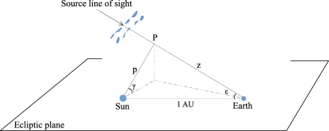
Figure 1.: Geometry of IPS observations. As the heliospheric equator nearly coincides with the ecliptic plane, the angle, $\gamma$, approximates to the heliographic latitude of the ‘P’ point.

3.1 Background Theory – Geometry of IPS Observation

Figure 1 illustrates a simplified geometry of IPS observations. The solar elongation, $\varepsilon$, is the angle between the Sun-Earth line and the line of sight to the radio source. This angle changes by approximately one degree per day due to the orbital motion of the Earth as the radio source appears to approach or recede from the Sun. IPS measurements represent the integrated effects of the solar wind along the total line of sight. However, the solar wind contribution is dominated by the region around the closest approach point of the line of sight, referred to as the ‘P’ point, at a distance ${\rm p}=\sin({\varepsilon})$ in AU (see Figure 1). This dominance occurs because of the concentrated density turbulence, $\delta n_{e}^{2}(R)$, around the region of the ‘P’ point, as on either side of this along the line of sight, it decreases even steeper than $\delta n_{e}^{2}(R)\propto R^{-4}$ (e.g., Armstrong and Coles 1978; Manoharan 1993; Asai et al. 1998; also see subsequent sections). The results on the radial dependence of the scintillation power obtained from this study during the initial minimum phase of the current solar cycle are discussed in Section 5.

3.2 Scintillation Index – Radial Dependence

The IPS of a source is quantified by its scintillation index, $m$, which is the rms of the intensity fluctuations normalized by the average intensity, $m\,=\,\{\langle\delta I(t)^{2}\rangle\}^{\frac{1}{2}}/\langle I\rangle$ (e.g., Hewish, Scott, and Wills 1964; Manoharan 1993). Since the rms of intensity fluctuations is equivalent to the square root of the integrated temporal power spectrum, the scintillation index $m$ can also be estimated by, $m=\left(\int P(f)\,{\rm d}f\right)^{\frac{1}{2}}/{\langle I\rangle}$. $P(f)$ is derived from the Fourier transform of the time series of intensity fluctuations, $I(t)$. The power level of the temporal spectrum is determined by the scattering strength, $C^{2}_{\delta n_{e}}(R)\propto R^{-\beta}$, which is integrated along the line of sight. With the scattering radial index, $\beta$, typically ranging from 4 to 4.5 (e.g., Armstrong and Coles 1978; Manoharan 1993; Asai et al. 1998; Manoharan 2012), the dominant contribution to scintillation arises from the solar wind plasma layers near the point of closest solar approach along the line of sight (see Figure 1).

The rms of intensity fluctuations, $\delta I(t)(R)$, increases as the Sun is approached. For a perfect coherent point source, the index, m, reaches a maximum value close to unity at a heliocentric distance, $R_{peak}$, and remains nearly at the same level (i.e., the saturated level) for closer distances. The distance of the saturation onset, $R_{peak}$, depends on the frequency of observation, and it moves closer to the Sun with increasing frequency of observation (Marians 1975; also see Section 5.2). For a finite source size, the index maximizes at $R_{peak}$, although $m_{peak}$ is always less than unity for a source of finite angular size. The $m$ then decreases for smaller solar offsets, due to the incoherency of scintillation caused by the source structure. As the angular scale size of the source increases, $m_{peak}$ decreases and completely vanishes, when the source’s angular size is much greater than the Fresnel scale. The maximum value of the index, $m_{peak}$, or the radial-dependence of the $m(R)$ curve, provides an estimate of the source size (e.g., Marians 1975; Manoharan 1993).

At distances $R~<~R_{peak}$, the scattering is ‘strong’. In contrast, at $R>R_{peak}$, the scattering is ‘weak’, and the index $m^{2}$ is linearly related to $\delta n_{e}^{2}$. The ‘m – R’ curve provides the radial dependence of the density fluctuations, $\delta n_{e}(R)$ (see Section 5).

3.3 Model IPS Temporal Spectrum

Under weak-scattering conditions, for a thin layer of solar wind plasma located at the closest solar approach plane perpendicular to the line of sight at a distance z from the observer, (i.e. on the x-y plane at the ‘P’ point), the contribution to the temporal spectrum includes an integral over the x-y plane, expressed as:

$$P(f,z)_{R=p}=\frac{(2\pi r_{e}\lambda)^{2}}{|V(z)|}\int^{+\infty}_{-\infty}{\rm d}\kappa\;\;C^{2}_{\delta n_{e}}(R)\cdot\Phi_{\delta{n_{e}}}(\kappa_{x},\kappa_{y},z)\cdot F_{diff}(\kappa,z)$$

$$\;\;\cdot F_{source}(\kappa,z,\theta_{o}),$$ (1)

where $\lambda$ is the observing wavelength, $r_{e}$ is the classical electron radius, and $\kappa$ is the wavenumber (Armstrong et al. 1990; Manoharan and Ananthakrishnan 1990). The scintillation is controlled by the angular size of the source, $F_{source}(\kappa,z,\theta_{o})$, the diffraction term, $F_{diff}(\kappa,z)$ (Fresnel-filter term), scaled by the radial velocity of the solar wind, $V(z)$, perpendicular to the signal path in the $z$ direction and the observation wavelength $\lambda$ (frequency, $\nu$). The resultant temporal spectrum, $P(f)$, is the sum of contributions of plasma layers between the observer and the source along the z direction, as given by:

$$P(f)=\int_{observer}^{\infty}P(f,z){\rm d}z.$$ (2)

The shape of the temporal spectrum reflects the spatial spectrum of intensity turbulence, $\Phi_{\delta{n_{e}}}(\kappa)\propto\kappa^{-\alpha}$. The diffraction term, $F_{diff}=\sin^{2}\left({\kappa^{2}}/{\kappa^{2}_{diff}}\right)=\sin^{2}\left({\kappa^{2}\lambda z}/{4\pi}\right)$, influenced by the observing wavelength, defines the Fresnel scale involved in scintillation. It introduces a knee-like feature around the Fresnel wavenumber, $\kappa_{diff}=\sqrt{4\pi/{\lambda z}}$. The corresponding temporal frequency, $f_{diff}=V(z)\,\kappa_{diff}/2\pi$, shifts to higher values as the solar wind radial velocity increases. For an isotropic distribution of density irregularities, the wavenumber $\kappa$ is defined as $\kappa=(\kappa_{x}^{2}+\kappa_{y}^{2})^{\frac{1}{2}}$, where x and y represent the radial and perpendicular directions, respectively.

In general, the scales of solar wind density turbulence are influenced by the radial expansion of the solar wind and the orientation of the mean magnetic field. If present, such anisotropy modifies the spectrum to $\Phi_{\delta n_{e}}(\kappa)\propto\left(\kappa_{x}^{2}+\frac{\kappa_{y}^{2}}{{\rm AR}^{2}}\right)^{-\alpha/2}$, where AR is the axial ratio of the density irregularities (e.g., Armstrong et al. 1990; Coles, Harmon, and Martin 1991; Grall et al. 1997; Yamauchi et al. 1998). An AR value greater than one results in the rounding of the Fresnel knee of the spectrum (e.g., Scott, Rickett, and Armstrong 1983; Manoharan, Ananthakrishnan, and Pramesh Rao 1987; Manoharan, Kojima, and Misawa 1994). The effect of the dissipative scale, $S_{i}$, is observed as a sharp decline in power at the high-frequency end of the temporal spectrum, $\exp(-\kappa^{2}/\kappa_{i}^{2})$, where $\kappa_{i}=3/S_{i}$ represents the inner-scale cutoff (e.g., Manoharan, Ananthakrishnan, and Pramesh Rao 1987; Coles, Harmon, and Martin 1991; Yamauchi et al. 1998); Manoharan et al. 2000; Spangler et al. 2002).

Both the observing bandwidth and the finite angular size of the source result in a decrease in source coherence, leading to a reduction in the overall level of scintillation, $m$ $<$ 1 (e.g., Little and Hewish 1966; Manoharan 1993). The Fourier transformation of the brightness distribution of a source having a finite angular size, i.e., the visibility function of the source, $\exp(-\kappa^{2}z^{2}\theta_{o}^{2})$ attenuates scintillation at high wavenumbers above $\kappa_{source}=(z\theta_{o})^{-1}$, where $\theta_{o}$ is the angular radius of the source at the $e^{-\frac{1}{2}}$ level (the full width at half maximum of the source brightness distribution, ${\Theta}\,=\,2.35{\theta_{o}}$) (e.g., Marians 1975; Coles 1978; Manoharan, Kojima, and Misawa 1994; Yamauchi et al. 1998). The Gaussian cutoff of the source size, $\theta_{o}\ll\sqrt{\lambda/z}$, occurring at frequencies $f_{source}\,=\,{\rm V_{sw}}/2\pi(z\theta_{o})$, primarily affects the high-frequency portion of the temporal spectrum. However, a source size of $\theta_{o}\gtrsim\sqrt{\lambda/z}$ can considerably lower the Fresnel knee of the spectrum, resulting in reduced power of the scintillations.

By fitting a multi-parameter model based on Equation (2) to the observed temporal spectrum, it is possible to derive the typical speed of the solar wind and the power-law characteristics of the turbulence spectrum (e.g., Manoharan and Ananthakrishnan 1990; Manoharan, Kojima, and Misawa 1994). When the signal-to-noise ratio of the power spectrum is significant in the high-frequency region, it can be useful for estimating the combined effect of the angular size of the radio source and the inner-scale size of the turbulence. Conversely, if the angular size of the source is known from the Very Long Baseline Interferometry (VLBI) observations, this spectral-fitting approach can provide estimates of the dissipative (or inner) scale of the turbulence (e.g., Manoharan, Ananthakrishnan, and Pramesh Rao 1987; Manoharan, Kojima, and Misawa 1994; Manoharan et al. 2000; Yamauchi et al. 1998).

4 Multi-frequency IPS – Results and Discussion

4.1 Frequency Dependence of Scintillation – Dynamic Spectrum

The wide frequency coverage of the IPS observations in the P-, L-, and S-bands ($\sim$300 – 3100 MHz) using the Arecibo telescope enables analysis of the frequency dependence of scintillation. Notably, the IPS recordings in the L-band, covering a broad range of $\sim$600 MHz, enable the investigation of scintillation variations in 10-MHz intervals. Figure 2 shows the L-band dynamic spectrum of IPS for the source B0742+103, observed on 12 July 2020. The solar elongation of the source was 12^∘, corresponding to $R$ $\approx$ 45 $R_{\odot}$. This plot presents a 30-s time series, after applying a 10-s running mean subtraction (i.e., 40-s data was included in the analysis). For each frequency channel, the scintillation index was computed from the rms of a 200-sample block (i.e., 200-ms data). The source deflection, $\langle I\rangle$, represents the difference between the mean levels of the on-source and off-source observations over the 30-s data.

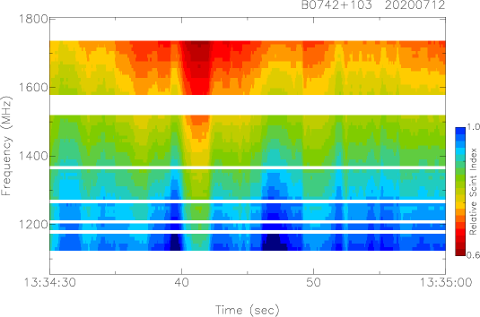
Figure 2.: Scintillation dynamic spectrum of B0742+103 observed with the Arecibo L-band system. The large white patch between 1520 and 1580 MHz is the gap in the L-band system and other smaller gaps at lower frequencies are due to interference.

In Figure 2, a prominent feature is the systematic decrease in the scintillation from the lower to the higher frequencies, illustrating the direct proportionality between scintillation and wavelength. Additionally, the random temporal variability of scintillation for each frequency band is evident along the time axis. The reduction in scintillation with increasing frequency is consistent with dynamic spectra observed in LOFAR data and numerically simulated spectra (Fallows et al. 2013; Coles and Filice 1984). However, such a systematic reduction was not clear when the observation covered the weak-to-strong scattering transition (e.g., Cole, Slee, and Hewish 1980).

The dynamic spectrum provides valuable insights into the influence of solar wind density microstructures that generate scintillation. As outlined in the following section, the frequency (or wavelength) dependence of scintillation is clearly revealed when examining the scintillation index, $m(\lambda,R)$, for each 10-MHz channel of the Arecibo bands.

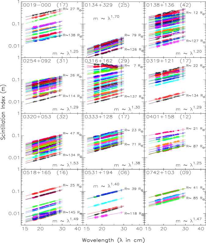
Figure 3.: The ‘$m$ – $\lambda$’ plots of multiple sources observed at L-band system. In each plot, m values measured on a day across the band are plotted by a distinct color, with the corresponding best-fit line. A vertical bar plotted at $\lambda$ = 29 cm on each day plot is the typical average error on the measured indices at the $\pm$1-$\sigma$ level. The number of days observed for each source is given in parentheses to the right of the source name.

4.2 L-band System – ‘$m$ – $\lambda$’ Plots

Figure 3 displays log-log plots of the scintillation index, $m$, as a function of wavelength, $\lambda$, across 56 channels, each with a 10-MHz bandwidth, from the L-band system. The figure includes data for 12 sources observed between March and August 2020. During this period, which marked the early minimum phase of solar cycle 25, solar activity was relatively quiet. These sources have scintillating flux densities, $\Delta S$ $>$ 1 Jy, at 327 MHz (Manoharan 2009; Manoharan 2012). The number of days of observations for each source ranged from 6 to 42, as indicated in parentheses next to the source name. Additionally, the minimum and maximum solar offsets for each source are shown, corresponding to the top (high $m$ day) and the bottom (low $m$ day) curves, respectively. For instance, the closest solar offset observation for source 0316+162 was at 7 $R_{\odot}$ in the strong scattering region, while the maximum solar offset was 137 $R_{\odot}$.

In the strong scattering regime, the $m-\lambda$ relationship differs from that in the weak scattering regime, which occurs at solar offsets $>$15 $R_{\odot}$. Specifically, at L-band at a central wavelength of $\lambda$ = 21 cm (frequency, $\nu$ = 1420 MHz), the scintillation index peaks around 10 – 15 $R_{\odot}$ (see Figure 8). Interestingly, at the solar offset of $\sim$7 $R_{\odot}$, on the longer wavelength side, the scintillation index reaches or crosses the turnover point, $R_{peak}$, and shows a decrease (refer to the plots of B0316+162 and B0138+136 in Figure 3). On the shorter wavelength side, the index approaches the turnover region, and the reduction in scintillation is significantly less than at the longer wavelengths. This wavelength dependence in the strong scattering region reveals intriguing characteristics, offering insights into the turbulence spectrum in strong (or saturated) scattering conditions and this will be dealt in a separate study.

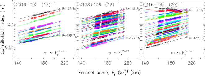
Figure 4.: Scintillation index plotted against the Fresnel scale for three very compact sources shown in Figure 3. The format and color scheme are similar to Figure 3. A vertical bar plotted at F_r = 210 km on each day plot is the average error on the measured indices at the $\pm$1-$\sigma$ level.

The IPS observations presented in Figure 3 include a range of heliocentric distances. It reveals that for a given source, the ‘$m$ – $\lambda$’ curves at different distances in the weak-scattering regime exhibit similar slopes. For each source, the average slope, $\omega$, ($m~\propto~\lambda^{\omega}$) obtained at heliocentric distances $>$20 $R_{\odot}$, is indicated. The index, $\omega$, ranges between 1.2 and 1.7. A higher index, i.e., a steeper ‘$m$ – $\lambda$’ curve, signifies a sharp drop in scintillation at shorter wavelengths or a steeper increase of $m$ at longer wavelengths. The day-to-day variation in $\omega$ values observed for a given source at different solar offsets can be primarily attributed to changes in $\delta n_{e}$.

Multi-wavelength IPS studies hold significant potential in the study of turbulence micro-scale structures. Since scintillation phenomena are governed by the Fresnel scale, $\sqrt{\lambda z}$, comparing scintillation as a function of the Fresnel scale can provide valuable insights into the scintillation scales at different observing wavelengths. This approach can also be beneficial for broad inter-comparisons of IPS observations from different radio sources at various frequencies. However, in line-of-sight integrated IPS observations, the distance to the scattering screen, $z$, is not a fixed parameter. The scattering screen can involve a finite thickness and is effectively determined by the solar wind layers located near the point of closest solar approach, the ‘P’ point (as illustrated in Figure A.1). At smaller solar offsets, $\varepsilon$ $<$ 45^∘, the maximum level of scattering is observed at $z=\cos(\varepsilon)$. Considering this caveat, the $m$ values for three sources, namely B0019-000, B0138+136, and B0316+162, are replotted in Figure 4, incorporating the effective $z$ at the ‘P’ point for each observation. For observations at large elongations, the effective scattering layer moves closer to the observer, with $z$ $<$ 1 AU. Consequently, the Fresnel scale associated with the effective screen distance becomes smaller. However, the ‘$m$ – $\lambda$’ and ‘$m$ – $\sqrt{\lambda z}$’ plots look nearly identical, and the slopes are also basically the same when the $\sqrt{\lambda}$ is considered (refer to Figure 3).

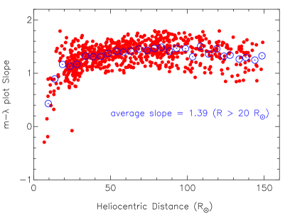
Figure 5.: Arecibo L-band IPS observations: The slope of ‘$m$ – $\lambda$’ curve plotted as a function of heliocentric distance.

4.2.1 The L-band System – Heliocentric Distance Dependence of ‘$m$ – $\lambda$’

The IPS observations with the Arecibo L-band system included a large number of sources in the heliocentric distance range of $\sim$6 – 150 $R_{\odot}$. Figure 5 shows the slope, $\omega$, of the ‘$m$ – $\lambda$’ dependency plotted against the heliocentric distance. In the strong scattering regime, the slopes are flatter than the weak-scattering curves. Whereas at distances $>$20 $R_{\odot}$, slope values range between $\sim$1 and 1.8, with an average of $\sim$1.39$\pm$0.2, which is consistent throughout the distance range covered. The 5-$R_{\odot}$ bin-averaged points are over plotted on the same figure and are shown as blue circles. We observe a mild peak around 80 $R_{\odot}$. The cause of this effect is currently unclear and will be investigated in detail in a future study.

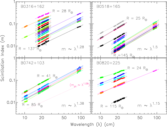
Figure 6.: The ‘$m$ – $\lambda$’ plots of four sources observed with the Arecibo P-, L-, and S-band systems. As in Figures 3 and 4, each day’s measured m values are plotted with a distinct color, along with their corresponding best-fit line. The dotted line shown along with curves of B0742+103 is the ‘$m_{pt}$ – $\lambda$’ curve of an ideal point source, obtained from the model spectra using Equation (2), for $\alpha$ = 3.3, $\varepsilon$ = 40^∘, AR =1, and $V_{sw}$ = 400 km s^-1.

4.3 Three Bands – ‘$m$ – $\lambda$’ Dependence

For some of the sources, the IPS have been monitored near simultaneously, i.e., within about 30 minutes, at P-, L-, S-band systems. Figure 6 displays the ‘$m$ – $\lambda$’ plots of four sources, B0316+162, B0518+165, B0742+103, and B0820+225. The format of this figure is similar to Figure 3. For the sources B0316+162 (CTA 21, a well-known compact quasar of angular size, $\Theta\approx 30~$mas) and B0518+165 (3C138, a compact quasar of size, $\Theta\approx 90~$mas), the $\omega$ indices are nearly the same as L-band observations (Figure 3). In contrast, for B0742+103, the average index obtained from the three-band observations is $\omega_{{}_{PLS}}$ = 1.38, which is flatter than the average index obtained with L-band alone, $\omega_{{}_{L}}$ = 1.47. B0742+103 is a GHz-peaked spectrum radio quasar at a high redshift of 2.624 (Kharb, Lister, and Cooper 2010). Most of its flux density is contained in a core of size less than 60 mas. Comparison of its ‘$m-R$’ dependence at the three-frequency bands suggests that the percentage of the scintillating flux at S-band is likely higher than at P-band, and it is consistent with the flux density peaking around 2.7 GHz. This likely leads to a flatter $\omega$ curve. BL Lacertae object B0820+225, located at a redshift of 0.951, exhibits a 5 GHz flux density of 1.6 Jy. Extensive imaging observations of this source have been made at various frequencies using the Very Long-Baseline Array (VLBA) and VLBI, specifically in the frequency range of 1.6 – 15 GHz. Approximately 30–40% of its flux density is associated with an elongated jet-like structure, measuring less than or about 30 mas (e.g., Pushkarev and Gabuzda 2001; Gabuzda, Pushkarev, and Garnich 2001). Over 300 interplanetary IPS observations were taken at 327 MHz using the Ooty Radio Telescope, spanning a range of solar elongations across different solar cycle phases. These observations revealed an average total flux density of approximately 4 Jy and a scintillation flux density of around 1.2 Jy (Manoharan 2009; Manoharan 2012). The average $\omega$ value of this source is flatter than the above-mentioned sources.

For reference, model spectra at the middle of the P, L, and S bands were computed using Equation (2) for both an ideal point source and a source with a size of 60 mas. These spectra are displayed in Figure A.2. For the point source, an $\omega$ value of 1.08 was obtained. The corresponding curve is displayed along with the B0742+103 data in Figure 6. The difference in power level between the point source spectrum and the finite source size spectrum progressively increases with decreasing wavelength (or increasing frequency). This results in an $\omega$ value of approximately 1.4 for the source size of 60 mas, which is consistent with the above results.

Earlier multi-frequency IPS studies have indicated the reduction of scintillation with frequency (e.g., Gapper and Hewish 1981; Scott, Rickett, and Armstrong 1983; Coles and Filice 1984; Bourgois et al. 1985; Breen et al. 2006; Fallows et al. 2006; Liu et al. 2010; Fallows et al. 2013; Morgan et al. 2017).

The observed range of $\omega$ values is consistent with the theoretically predicted dependences of $\omega$ = 1.45 and $\omega$ = 1.25, obtained by Armand, Efimov, and Yakovlev (1987), respectively, corresponding to density turbulence described by a Kolmogorov spectrum with $\alpha$ = 11/3 and a less steep spectrum with $\alpha$ = 3. As the spectral power decreases more rapidly with increasing temporal frequency, the value of $\omega$ also tends to increase.

Spacecraft observations have shown that the spectral index, $\alpha$, evolves with distance from the Sun. In the near-Sun region ($R$ $<$ 16 $R_{\odot}$), for the density-irregularity scale sizes considered in the present IPS observations, an average $\alpha$ $\approx$ 3 has been observed. This steepens to a range of approximately 3.3 – 3.4 at distances between $\sim$20 and 100 $R_{\odot}$. At larger solar offsets, $R$ $>$ 100 $R_{\odot}$, the spectral index $\alpha$ typically reaches a value around 3.7 (e.g., Woo and Armstrong 1979; Yakovlev et al. 1980; Armand, Efimov, and Yakovlev 1987; Celnikier, Muschietti, and Goldman 1987). Average $\omega$ values in this study are based on observations at heliocentric distances between 20 and 150 $R_{\odot}$. While the full range was considered, the most of observations were concentrated at distances below 100 $R_{\odot}$. Specifically, at frequencies of L band and higher, only compact sources produce measurable scintillation beyond 100 $R_{\odot}$. When day-to-day solar wind changes are mitigated, the effect of source size on the average $\omega$ cannot be disregarded.

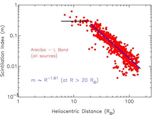
Figure 7.: The ‘$m$ – $R$’ plot of all sources observed with the Arecibo L-band system. The solid ‘blue’ line represents the straight-line fit to data points at distances $>$20 $R_{\odot}$, while the horizontal black line indicates the average value of $m$, approximately 0.3, for distances $\leq$15 $R_{\odot}$.

5 Radial Dependence of Scintillation

5.1 L-band Observations

Figure 7 displays the plot of ‘$m$ – $R$’ of the L-band observations for all sources observed, covering the distance range of $\sim$6 – 150 $R_{\odot}$. For each source scan in a day, the mean scintillation index has been obtained by averaging over the available 10-MHz channels. Thus, it represents the scintillation index at the middle of the L-band, $\sim$1420 MHz (refer to Figures 3 to 5). The scintillation index increases as the source approaches the Sun (refer to Section 3.1). The saturation level of scintillation, i.e., the onset of the strong scattering region, is expected at distances $\lesssim$20 $R_{\odot}$. Since there are fewer points for smaller solar offsets, and these include sources of different angular sizes as well as reduced level of $\delta n_{e}^{2}$ in the high-latitude coronal hole regions, the turnover of the scintillation index is not seen clearly. For example, in high-latitude regions, the level of scintillation at a given distance will be less than the level observed at the same distance in the equatorial or low-latitude regions (e.g., Manoharan 1993; Imamura et al. 2014; Coles 1996). At distances $\leq$15 $R_{\odot}$, the $m$ values range between 0.2 and 0.6 and the average ($m$ $\approx$ 0.3) is shown by a horizontal black line.

The least-square straight-line fit to the $m$ values, at distances $>$20 $R_{\odot}$, provides a relationship, $m~\approx~30\times{\rm R}^{-1.6}$. This is shown as a continuous blue straight line in Figure 7. The ‘$m$ - R’ dependence agrees with the results obtained from the 327-MHz IPS observations, made with the Ooty Radio Telescope, in the distance range of $\sim$40 – 215 $R_{\odot}$, for the minimum phases of solar cycles 20 to 24 (Manoharan 1993; Manoharan 2012) and other earlier IPS observations (e.g., Armstrong and Coles 1978; Asai et al. 1998).

5.2 Three Bands – ‘$m$ – R’ Dependence

Figure 8 (left) shows an example of the ‘$m$ – R’ plots of B0316+162 (CTA 21) at the three Arecibo bands. As mentioned above, the observations at P and S bands were limited in number, and only a few sources were covered at all three bands. Moreover, since the Arecibo P-band observations did not include distances in the turnover region (i.e., at the onset of strong scattering), the m values of B0316+162, measured using the Ooty Radio Telescope at 327 MHz during the declining phase of solar cycle 24 in 2018, are plotted for comparison. The Arecibo points agree with the Ooty observations for the overlapping distance range.

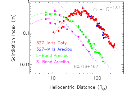
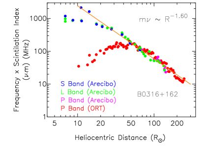
Figure 8.: (Left) The ‘$m$ – $R$’ plot of the compact source B0316+162, corresponding to the center frequencies of Arecibo P- L-, and S-band systems for the year 2020. For comparison, $m$ values observed at 327-MHz for the year 2018 with the Ooty Radio Telescope (ORT) are also plotted. (Right) The scintillation indices, $m$, multiplied by their corresponding observing frequencies ($m\cdot\nu$) are plotted. In both plots, the least-square fits to the data points in the weak-scattering region are shown as straight lines (also refer to Figure 9 (right), which shows ‘$m/\lambda^{\omega}$ – $R$’ plot).

The turnover of scintillation at 327 MHz is observed at $\sim$45 $R_{\odot}$. Whereas at L-band, it shifts to about 15 – 20 R_⊙. Since the number of observations at S-band is limited, and the turnover is not clear, we can only say that it is at $\lesssim$10 $R_{\odot}$. The least-square fitting to the weak-scattering regions at the three bands provide an essentially identical radial dependence of $m\propto R^{-1.6}$. The analytical solution of the line-of-sight integral, $\delta n_{e}^{2}(R)~\propto~R^{-S}$, leads to a radial index $S$ = (2$\times$1.6)+1, resulting in $\delta n_{e}^{2}(R)~\propto~R^{-4.2}$.

As the source B0316+162 approached the Sun, the ‘P’ points probed the high-latitude southern polar region of the heliosphere, at a heliographic latitude of about $-$80^∘ S. During the minimum phase of the current cycle, the high-latitude regions on the Sun were dominated by a large coronal hole of low density (see the Carrington map, CR2230, in the 193 Å channel of the Atmospheric Imaging Assembly (AIA) on board the Solar Dynamics Observatory (SDO) provided at https://sdo.gsfc.nasa.gov/data/synoptic/). The low-density turbulent solar wind emanating from this open-field region tends to move the onset of the strong-scattering region towards the Sun. Considering the above distance dependence of $\delta n_{e}^{2}(R)\sim R^{-4.2}$, a given level of scattering strength at the high-latitude region is observed at a distance closer than that of the equatorial region. This is consistent with the results of earlier remote-sensing studies (Manoharan 1993; Coles 1996; Manoharan 2012; Imamura et al. 2014).

The multi-frequency IPS technique employed in this study, especially at higher frequencies, allows us to overcome the limitation imposed by Fresnel filtering at meter-wavelengths. It enables the investigation of low-frequency temporal variations in ${\delta n_{e}^{2}}(R,z)$, as close as $\sim$10 $R_{\odot}$ at S-band, and provides valuable insights into the density turbulence.

5.3 Radial Dependence of Frequency-Scaled Scintillation Index

Figures 3 to 6 demonstrate the invariance of the ‘$m$ – $\lambda$’ dependence with the distance from the Sun. If the angular size of the source does not vary with the observing frequency, $\nu$, the product $m\cdot\nu$ is expected to yield a frequency (or wavelength) independent density turbulence (e.g., Readhead 1971). Figure 8 (right) shows the plot of $m\cdot\nu$, for the source B0316+162 as a function of heliocentric distance. The linear fit in the weak-scattering region extends from large to small solar offsets, i.e., from P- to S-bands, and the collective radial dependence remains the same as observed at each individual band.

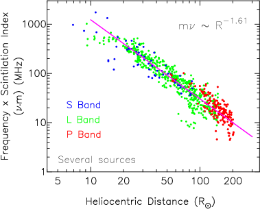
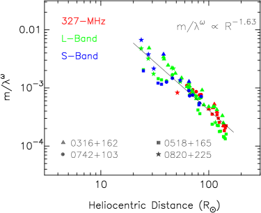
Figure 9.: (Left) Similar to Figure 8, the ‘$m\cdot\nu$ - $R$’ plot of all sources observed with Arecibo’s P-band (red dots), L-band (green dots), and S-band (blue dots) systems. The least-square fit to the observed data is shown as a straight line. (Right) The ‘$m/\lambda^{\omega}\sim R$’ plot for the four sources shown in Figure 6. Each source’s symbol is indicated, and the frequency-band color code is the same as in the left plot.

Similar to the B0316+162 plot, Figure 9 (left) presents the ‘$m\cdot\nu$ - $R$’ plot for all sources observed with the three Arecibo bands. The best linear fit for the measurements at three bands demonstrates the consistency in the radial dependence. It is also in agreement with the result of multiple-source observations presented in Figure 2 of Readhead (1971), $m\cdot\nu\propto R^{-1.59}$. Figure 9 (right) presents a plot of ‘$m/\lambda^{\omega}\sim R$’ for the four sources shown in Figure 6. The radial index exhibits consistent behavior for these sources. However, the data points associated with B0518+165 lie below the best-fit line, likely due to its larger angular size compared to the other sources considered.

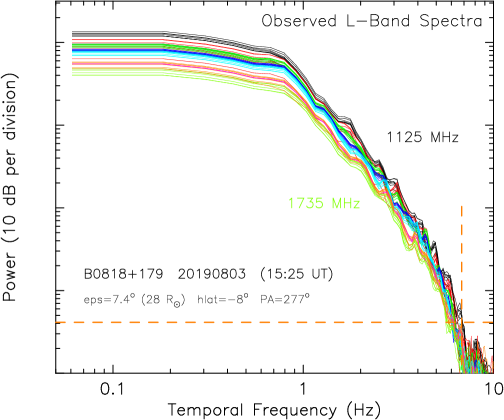
Figure 10.: Temporal power spectra of 56 channels at L-band, between 1125 and 1735 MHz, for the source B0818+179 on 3 August 2019. Each spectrum is separated by 10 MHz. Spectra within an 80-MHz band, (eight channels corresponding to one Mock box), are represented by a single color. The horizontal dashed line indicates the spectral off level where the scintillation power drops to the background noise level, while the vertical dashed line indicates the frequency at which this occurs. The off-level spectrum has been subtracted from the power spectrum.

6 Frequency Dependence of the Temporal Power Spectrum

6.1 L-band Observations

Following the systematic decreasing trend observed in the ‘$m$ – $\lambda$’ relationship (see Section 4.1 and Figures 3 to 5), a comprehensive analysis has been performed to investigate the evolution of the temporal spectrum at the three bands of the Arecibo system. Figure 10 displays the shapes and power levels of the temporal power spectra between 1125 and 1735 MHz for the source B0818+179. The observations were taken on 3 August 2019, at a solar elongation, $\varepsilon$ = 7.4^∘ (R $\approx$ 28 $R_{\odot}$), when the Sun–P-point position angle was 277^∘. The position angle, PA, is measured counterclockwise from the north pole. Each spectrum corresponds to a 10-MHz channel, and a total of 56 spectra are plotted. The maximum of each spectrum has been normalized to that of the spectrum at the lowest frequency, 1125 MHz, and the power level decreases from 1125 to 1735 MHz. Spectra within an 80-MHz band, (eight channels corresponding to one Mock box), are represented by a single color. A vertical dashed line marks the frequency at which the scintillation equals the system noise. Above this ‘cutoff’ frequency, the spectrum is nearly flat, resembling white noise. The horizontal line indicates the white-noise level, which has been subtracted from the power spectrum.

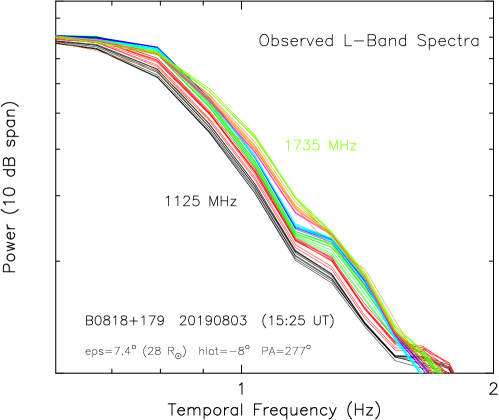
Figure 11.: Progressive broadening of the temporal spectrum with the observing frequency. Each spectrum plotted in Figure 10 has been normalized to a maximum level and plotted on an enlarged scale to show the increasing width of the spectrum with the frequency of observation. The color scheme is same as Figure 10.

In the above spectra, the flat spectral part at temporal frequencies below 0.7 Hz is caused by the rising part of the first Fresnel oscillation of the propagation filter combined with the power-law form of the spatial spectrum of density turbulence, given by $\sin^{2}\left({\kappa^{2}}/{\kappa^{2}_{diff}}\right)$ $\times$ $\left(\kappa_{x}^{2}+\frac{\kappa_{y}^{2}}{{\rm AR}^{2}}\right)^{-\alpha/2}$ (refer to Equation (2) in Section 3.3). The sharp ‘knee-like’ feature following the flat portion, where most of the turbulent power is contained, is known as the ‘Fresnel knee’. It is caused by the first minimum of the Fresnel oscillation. Integration along the line of sight tends to smooth out the higher-order Fresnel oscillations. It also alters the systematic slope at frequencies above the knee, i.e., the inertial part of the spectrum, to a power-law index of $\alpha$–1 (e.g., Manoharan, Kojima, and Misawa 1994).

The anisotropic turbulence structure (axial ratio, AR $>$ 1), if present, can reduce the amplitude of Fresnel oscillations, causing the ‘knee’ region to become rounded. The visibility function of the source, $\exp[-(\kappa z\Theta/2.35)^{2}]$, and the dissipation or inner-scale size of the turbulence ($S_{i}$), $\exp(-\kappa^{2}/{\kappa_{i}^{2}})$, where $\kappa_{i}$ = 3/$S_{i}$, effects become noticeable only at high temporal frequencies. For instance, a source with an angular width of $\Theta$ = 30 mas attenuates spatial wavenumbers $\kappa_{source}~>~0.1$ km^-1, resulting in reduction of power at temporal frequencies $>$ 7 Hz for a solar wind velocity of 400 km s^-1. At the current heliocentric distance, 28 $R_{\odot}$, the inner-scale cutoff will also be comparable to the source-size effect (Manoharan, Ananthakrishnan, and Pramesh Rao 1987; Coles, Harmon, and Martin 1991).

Since the frequency of the knee is linearly proportional to the solar wind velocity, expressed as $f_{knee}=V_{SW}/\sqrt{\pi\lambda z}$, the knee position shifts inward or outward along the frequency axis with a decrease or increase of the solar wind velocity. When the velocity remains constant, the temporal power spectra are expected to broaden progressively with observing frequency. This effect is clearly demonstrated in Figure 11, where the spectra are normalized to the maximum power level. This provides an enlarged view of the spectra, particularly in the region of the knee, and demonstrates the spectral broadening.

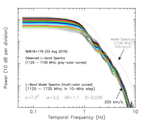
Figure 12.: Set of best-fitted model spectra computed using Equation (2) plotted in multi-color for a solar wind velocity of $V_{SW}=325$ km s^-1. In the background, the observed spectra are plotted in ‘gray color’. The model spectra are plotted with the same color scheme followed in Figure 10. To demonstrate the solar wind velocity scaling of temporal spectrum, a sample model spectrum at an observing frequency of 1735 MHz, for $V_{SW}=475$ km s^-1, is shown in a dotted line. Model parameters used in the computation are indicated.

6.2 L-Band Model Temporal Spectra

The best-fit model spectra for the L-band spectra displayed in Figure 10 have been obtained using Equation (2) and are displayed in Figure 12. For each 10-MHz band, the fitted parameters are: solar wind velocity, $V_{SW}$ = 325 km s^-1, power-law index, $\alpha$ = 3.3, axial ratio, AR = 1.1, and source size, $\Theta$ = 30 mas. Model spectra are plotted using the same color scheme as for the observed spectra in Figure 10. For comparison, the observed spectra are replotted in gray color in the background. Overall, a good agreement is found between the observed and model spectra, with the latter closely reproducing key features such as power levels, Fresnel knees, oscillations, and temporal-frequency scaling. However, a systematic deviation is observed at the knee region. Specifically, compared to the narrower frequency spread of the model knees, the observed spectra at low L-band frequencies are shifted towards higher temporal frequencies, while high-frequency observed spectra are shifted towards lower temporal frequencies.

6.2.1 Effective Width of the Temporal Spectrum – Spectral Moments

The width of the observed temporal spectrum, especially around the knee, has been carefully analyzed and compared to the model spectrum. The first moment, i.e., the area under the spectrum, represents the total variance integrated over all temporal frequencies, $\sigma^{2}={\int_{0}^{f_{c}}\,P(f)\,{\rm d}f}$, where $f_{c}$ is the cutoff frequency at which the scintillation power roughly drops to the noise level of the receive system (refer to Figure 10). Higher-order moments, normalized by $\sigma^{2}$, provide information about effective spectral widths at different power levels. The n^th-order spectral moment is defined as,

$$f{{}_{n^{\rm th}}^{n}}={\frac{1}{\sigma^{2}}}{\int_{0}^{f_{c}}\,f^{n}P(f)\,{\rm d}f}.$$ (3)

The second and third moments are particularly useful for understanding the spectral width within about the 2 – 5 dB down level of the spectrum, where the Fresnel knee is prominent, containing the most turbulent power, and can be used to infer the underlying physical processes affecting spectral broadening.

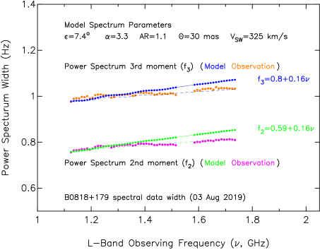
Figure 13.: Spectral widths (i.e., second ($f_{2}$) and third ($f_{3}$) moments) of the observed spectra, for the 56 channels of the L-band system (i.e., the spectra shown in Figure 10) are plotted against the observing frequency, $\nu$ in GHz. For comparison, widths of model spectra (shown in Figure 12) and spectra with progressively increasing axial ratio (see text) are plotted.

In Figure 13, the second and third moments calculated using Equation (3) for the 56-channel model spectra are plotted against the observing frequency, $\nu$ (in GHz) as green and blue dotted lines, respectively. A systematic broadening of the effective spectral width with increasing observing frequency is clearly seen. Both the second and third moments exhibit linear relationships with the same slope of $\sim$0.16 but differ by a constant offset of 0.21 Hz. The 3-dB down widths of the spectra fall between the curves of the second and third moments. The second-moment widths of the observed spectra, shown as ‘pink’ dots, align with the model spectra at lower observing frequencies, but systematically deviate toward lower widths at higher frequencies. Similar deviations are also noted in the third-moment widths, represented by ‘orange’ dots.

Since the model spectra were computed with a fixed axial ratio of AR = 1.1, the systematic deviation of the spectral width toward lower temporal frequencies with increasing observing frequency suggests that the axial ratio increases with the observing frequency. Another set of model spectra was computed, considering a linear increase in the axial ratio of about 20% over the frequency range of the L-band, while keeping the other model parameters unchanged. The spectra of the second and third moments, obtained from Equation (3), are plotted as green and blue dashed lines in Figure 13. At lower observing frequencies, the spectral widths align with the model spectra for the fixed axial ratio, and the gradual deviation of the moments with observing frequency agrees with the observed spectral moments. The results showing an increase in axial ratio with observing frequency (or a decrease with observation wavelength) suggest that anisotropy increases as the diffraction-scale size, $\sqrt{\lambda z}$, becomes smaller. Conversely, larger turbulent structures tend to be isotropic.

6.3 Temporal Spectra of Three Bands

Figure 14 presents the temporal spectra of the source B0820+225 for the three Arecibo bands, observed between 15:30 – 16:00 UT on 8 August 2020. The source had an elongation of $\varepsilon=14^{\circ}$, corresponding to a heliocentric distance of 51 $R_{\odot}$, with a PA of 299^∘, and a heliographic latitude of 17^∘. Each spectrum, shown as a thick-dotted line, represents the average of the band after subtracting its off-level spectrum, indicated by a dashed line.

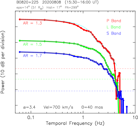
Figure 14.: Average spectra observed at P-, L-, and S-bands for B0820+225 on 8 August 2020 at a heliocentric distance of 51 $R_{\odot}$ ($\varepsilon$ = 14^∘). The horizontal dashed lines are the off-level spectra, corresponding to each band, which have been subtracted from the appropriate spectrum. The thin line overplotted on each spectrum is the best-fit model spectrum, and for which model parameters are indicated.

As exhibited by the ‘$m$ – $\lambda$’ plot for this source in Figure 6, a clear reduction in scintillation power of $\sim$20 dB ($P(f)\propto m^{2}$) between the P and S bands is revealed in the above spectra. The spectrum for each band has been fitted with the model spectrum obtained using Equation (2) and the best-fit model is over-plotted as a thin line on the observed spectrum. Model parameters include the power-law index of $\alpha$ = 3.3, a solar-wind velocity of $V_{SW}$ = 700 km s^-1 and a source angular size of $\Theta$ = 40 mas. However, the fitted axial ratios for the P-, L-, and S-bands are 1.3, 1.6, and 1.7, respectively. This progressive increase in axial ratio from low to high observing frequency indicates the consistency with the L-band results (Figures 12 and 13), confirming that turbulence scales become more anisotropic at smaller scales. The fitted solar wind velocity of $\sim$700 km s^-1 is consistent with the foot-point location of point ‘P’ on a low-emitting large unipolar region and its embedded coronal hole, which persisted for several days around the $\pm$30^∘ latitude region of the solar equator (refer to the SDO/AIA images in the 211 Å channel about a day before the observation date, allowing the solar-wind propagation time to the ‘P’ point; e.g., https://sdo.gsfc.nasa.gov/assets/img/browse/2020/08/07/20200807˙084811˙2048˙0211.jpg).

To examine spectral broadening between bands, the spectra have been normalized to a common power level and are displayed in Figure 15. For the P band, individual 10-MHz spectra are shown. For the L and S bands, average spectra from 80-MHz bands (each Mock box corresponds to eight channels, each of 10-MHz bandwidth) are plotted. The horizontal dashed lines indicate the average off-level spectra and each of it has been subtracted from the corresponding plotted spectrum. The temporal-frequency broadening between the P and L bands is evident over the entire frequency range beyond the Fresnel knee. However, due to increased rounding of the knees at the L and S bands, only marginal broadening between these is seen at approximately the 15-dB down level.

7 Summary and Conclusions

Interplanetary scintillation observations obtained from the Arecibo 305-m Radio Telescope with the P-, L-, and S-band systems in the frequency range of $\sim$300 – 3100 MHz have been analyzed. These observations covered a heliocentric distance range of $\sim$5 – 200 $R_{\odot}$ in the minimum phase at the end of solar cycle 24 and the beginning of cycle 25.

The scintillation dynamic spectrum obtained from L-band observations over a frequency range of $\sim$600 MHz permits the tracking of systematic reductions in density turbulence within this continuous band. The observed level of scintillation at a given frequency is closely associated with the density turbulence present in the corresponding micro-scale structures of the solar wind. The result agrees with the IPS dynamic spectra observed with LOFAR in the frequency range of 210 – 250 MHz, as well as simulated spectra (Fallows et al. 2013; Coles and Filice 1984). However, when dynamic spectra were observed in the strong scattering region, the aforementioned systematic trend in scintillation was not clear (Cole, Slee, and Hewish 1980; Hewish 1989; Fallows et al. 2013).

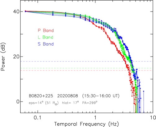
Figure 15.: Spectra of the source B0820+225, observed at three bands.

The dependence of the scintillation index, $m$, on the wavelength of observation, $\lambda$, has been quantitatively examined based on the estimation of $m$, at frequency intervals of 10 MHz, for many sources at the L band, along with near-simultaneous observations of selected sources covering the P-, L-, and S-band systems. There is a systematic dependence of $m\sim\lambda^{\omega}$. For a given source, the index, $\omega$, remains relatively constant for observations made at different heliocentric distances within the weak-scattering limit. The values of $\omega$ fall between $\sim$1 and 1.8 and this range is based on observations of several sources. For a given source, the day-to-day variation of $\omega$ is primarily due to the changes of density turbulence along different lines of sight (refer to Figures 3 to 6). However, the average value of $\omega$ of a source, obtained from observations taken on different days, typically represents the angular size associated with the source.

The consistency of the ‘$m$ – $\lambda$’ dependence with the distance from the Sun allows a study of the solar wind density turbulence in the near-Sun region, extending as close as $\sim$10 $R_{\odot}$, particularly when using S-band observations. Since the rms of density fluctuations, $\delta n_{e}$ is related to $m^{2}(\theta_{o},\lambda)\sim\lambda^{2w}\int_{z}\delta n_{e}^{2}(R,\lambda,z,\theta_{o})\;{\rm d}z$. Thus, the level of rms density fluctuations giving rise to scintillation is controlled by the density scale size relative to the Fresnel scale present in the solar wind. Since in the weak-scattering region, the $\delta n_{e}$ and $m$ are linearly related, the high-frequency observations allow to study the correlation between them in the near-Sun region.

The reduction of scintillation with the wavelength of observation has been reported in earlier multi-frequency IPS studies, which also include the decrease of correlation observed with dual-frequency measurements (e.g., Gapper and Hewish 1981; Scott, Rickett, and Armstrong 1983; Coles and Filice 1984; Bourgois et al. 1985; Breen et al. 2006; Fallows et al. 2006; Liu et al. 2010; Fallows et al. 2013; Morgan et al. 2017).

The present study provides the radial evolution of $m$ with heliocentric distance at three separate bands. The shifting of the weak-to-strong scattering transition region closer to the Sun from low to high frequency is clearly illustrated in Figures 7 to 9. Specifically, high-frequency observations effectively allow us to probe the solar wind closer to the Sun, where the linear relationship between $m$ and $\delta{n_{e}}$ is maintained. The invariance of the ‘$m$ – $\lambda$’ relationship with the heliocentric distance has been effectively demonstrated by the $m$ measurements at each individual band (also $m$ scaled with frequency of observation, $m\cdot\nu$ or $m/\lambda$), Figures 8 and 9. Such multi-frequency IPS measurements are relatively rare in previous studies (e.g., Cohen and Gundermann 1969; Readhead, Kemp, and Hewish 1978). During the current solar cycle minimum, the observed radial variation of $\delta n_{e}^{2}(R)\sim R^{-4.2}$ is consistent with earlier results (Manoharan 1993; Asai et al. 1998; Manoharan 2012).

In addition to the ‘$m$ – $\lambda$’ relationship, the temporal power spectrum analysis, for 10-MHz intervals of the L-band IPS, indeed for all three P-, L-, and S-bands, has shown a systematic decrease of the power level and frequency broadening of the spectrum with increasing observing frequency. The best-fit model to the observed spectrum allowed us to infer the typical solar wind velocity and the spatial spectrum of density turbulence, i.e., power-law index, $\alpha$. However, the model-fitting procedure revealed a systematic deviation of the Fresnel knee of the spectrum, toward the low frequency, with the observing wavelength. Careful examination indicates that the spectrum involved with the large-scale size has been associated with more isotropic turbulence scale than the small-scale spectrum. The axial ratio increases as the scale size of turbulence responsible for the scintillation decreases.

The above result is consistent with the increase of field-aligned anisotropy as the Sun is approached, at heliocentric distance $<$20 $R_{\odot}$, where the scale size decreases with solar offset (e.g., Armstrong et al. 1990; Grall et al. 1997). Additionally, a recent investigation of the solar wind at 1 AU, based on the Advanced Composition Explorer (ACE) mission in-situ data, showed that the density correlation scale in the direction quasi-parallel to the mean magnetic field is slightly larger than that in the quasi-perpendicular direction (Wang et al. 2024). Moreover, some of the simulations and theoretical studies have confirmed the increased anisotropy with decreased scale size (e.g., Shebalin, Matthaeus, and Montgomery 1983; Beresnyak, Lazarian, and Cho 2005; Oughton and Matthaeus 2005). The multi-frequency IPS observations presented in this study highlight the significance of probing the characteristics of solar wind density turbulence at various spatial scales and distances from the Sun.

During these multi-frequency IPS observing sessions, some weak CME events were also detected. These observations are valuable for understanding CME propagation in the inner heliosphere. Additionally, the high sensitivity of the Arecibo telescope provided spectra extending to high temporal frequencies, enabling estimation of the inner scale of turbulence for sources with known VLBI source-size structures. The results of these investigations will be presented elsewhere.

Acknowledgements

We thank the observational, computational, and engineering support provided by Phil Perillat, Arun Venkataraman and other staff members of the Arecibo Observatory. The Arecibo Observatory was operated by the University of Central Florida under a cooperative agreement with the National Science Foundation, and in alliance with Universidad Ana G. Méndez and Yang Enterprises, Inc. We also thank the observing team of the Radio Astronomy Centre (RAC) for the 327-MHz IPS observations. The RAC is run by the National Centre for Radio Astrophysics of the Tata Institute of Fundamental Research, India. PKM wishes to thank Tapasi Ghosh for numerous useful discussions and suggestions during the preparation of the manuscript.

Funding The Arecibo Observatory was operated by the University of Central Florida under a cooperative agreement with the National Science Foundation (grant number: AST-1822073), and in alliance with Universidad Ana G. Méndez and Yang Enterprises, Inc. PKM acknowledges support from the University of Central Florida. He also acknowledges support from NASA GSFC through the Cooperative Agreement to the Catholic University of America in support of the Partnership for Heliophysics and Space Environment Research (PhaSER) under the grant 80NSSC21M0180. CJS did not receive funding for this work.

Data Availability The observed IPS datasets analyzed in the current study are available at the Arecibo Observatory data archive maintained at the Texas Advanced Computing Center (www.tacc.utexas.edu/about/help/). The temporal power spectra generated during the current study are available from the corresponding author on request.

Declarations

Competing interests The authors declare no competing interests.

Appendix A Supplementary Figures

This appendix contains some additional figures to support the results described in Section 4.

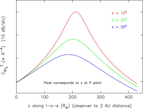
Figure A.1.: Scattering level plotted as a function of distance, z (along the line of sight), from the observer to 2 AU, on a ‘log-linear’ scale. The plots are shown for three elongations as indicated. For these plots, the $\beta$ value of $-$4 has been used in the power-law dependence of $C^{2}_{\delta n_{e}}(R)\propto R^{\beta}$. For each elongation, the peak in the scattering level corresponds to the location of the solar-wind layer at the ‘P’ point.

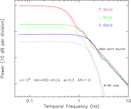
Figure A.2.: Model spectra at the middle of the P-, L-, and S-bands, computed using Equation (2). Solid lines and dotted lines represent an ideal point source and a source with a size of 60 mas, respectively. The model parameters used in the computation are indicated. In this log-log plot, the difference in power level between the point source spectrum and the finite source size spectrum progressively increases with decreasing wavelength (or increasing frequency). The derived $\omega$ values are 1.08 for the point source and 1.4 for the finite source.

References

- Altschuler and Salter (2013) Altschuler, D.R., Salter, C.J.: 2013, The Arecibo Observatory: Fifty astronomical years. Physics Today 66, 43. DOI. ADS.
- Armand, Efimov, and Yakovlev (1987) Armand, N.A., Efimov, A.I., Yakovlev, O.I.: 1987, A model of the solar wind turbulence from radio occultation. A&A 183, 135. ADS.
- Armstrong and Coles (1978) Armstrong, J.W., Coles, W.A.: 1978, Interplanetary scintillations of PSR 0531+21 at 74 MHz. ApJ 220, 346. DOI. ADS.
- Armstrong et al. (1990) Armstrong, J.W., Coles, W.A., Kojima, M., Rickett, B.J.: 1990, Observations of Field-aligned Density Fluctuations in the Inner Solar Wind. ApJ 358, 685. DOI. ADS.
- Asai et al. (1998) Asai, K., Kojima, M., Tokumaru, M., Yokobe, A., Jackson, B.V., Hick, P.L., Manoharan, P.K.: 1998, Heliospheric tomography using interplanetary scintillation observations 3. Correlation between speed and electron density fluctuations in the solar wind. J. Geophys. Res. 103, 1991. DOI. ADS.
- Baron et al. (2024) Baron, G., Aguilar-Rodriguez, E., Mejia-Ambriz, J.C., Chang, O., Gonzalez-Esparza, J.A., Villanueva, P., Andrade, E.: 2024, An updated catalog of IPS radio sources observed by MEXART at 140 MHz for space weather studies. Journal of Atmospheric and Solar-Terrestrial Physics 257, 106208. DOI. ADS.
- Beresnyak, Lazarian, and Cho (2005) Beresnyak, A., Lazarian, A., Cho, J.: 2005, Density Scaling and Anisotropy in Supersonic Magnetohydrodynamic Turbulence. ApJ 624, L93. DOI. ADS.
- Bisi et al. (2009) Bisi, M.M., Jackson, B.V., Clover, J.M., Manoharan, P.K., Tokumaru, M., Hick, P.P., Buffington, A.: 2009, 3-D reconstructions of the early-November 2004 CDAW geomagnetic storms: analysis of Ooty IPS speed and density data. Annales Geophysicae 27, 4479. DOI. https://angeo.copernicus.org/articles/27/4479/2009/.
- Bisi et al. (2010) Bisi, M.M., Jackson, B.V., Fallows, R.A., Dorrian, G.D., Manoharan, P.K., Clover, J.M., Hick, P.P., Buffington, A., Breen, A.R., Tokumaru, M.: 2010, Solar Wind and CME Studies of the Inner Heliosphere Using IPS Data from Stelab, ORT, and EISCAT. In: Advances in Geosciences, Volume 21: Solar Terrestrial (ST) 21, 33. DOI. ADS.
- Bisi et al. (2021) Bisi, M.M., Pacini, A., Aguilar-Rodriguez, E., Tokumaru, M., Gonzalez-Esparza, A., Jackson, B., Fallows, R., Fujiki, K., Yan, Y., Manoharan, P.K., Chashei, I., Tyulbashev, S., Iwai, K., Barnes, D., Chang, O., Robertson, S.: 2021, A Ground-Based Heliospheric Observatory for Space Weather: The Worldwide Interplanetary Scintillation (IPS) Stations (WIPSS) Network. In: 43rd COSPAR Scientific Assembly. Held 28 January - 4 February 43, 2370. ADS.
- Bourgois et al. (1985) Bourgois, G., Daigne, G., Coles, W.A., Silen, J., Turunen, T., Williams, P.J.: 1985, Measurements of the solar wind velocity with EISCAT. A&A 144, 452. ADS.
- Breen et al. (2006) Breen, A.R., Fallows, R.A., Bisi, M.M., Thomasson, P., Jordan, C.A., Wannberg, G., Jones, R.A.: 2006, Extremely long baseline interplanetary scintillation measurements of solar wind velocity. Journal of Geophysical Research: Space Physics 111. DOI. https://agupubs.onlinelibrary.wiley.com/doi/abs/10.1029/2005JA011485.
- Celnikier, Muschietti, and Goldman (1987) Celnikier, L.M., Muschietti, L., Goldman, M.V.: 1987, Aspects of interplanetary plasma turbulence. A&A 181, 138. ADS.
- Chashei et al. (2023) Chashei, I.V., Tyul’bashev, S.A., Lukmanov, V.R., Subaev, I.A.: 2023, ICMEs and CIRs monitored in IPS data at a frequency of 111 MHz. Advances in Space Research 72, 5371. DOI. ADS.
- Chhetri et al. (2018) Chhetri, R., Morgan, J., Ekers, R.D., Macquart, J.-P., Sadler, E.M., Giroletti, M., Callingham, J.R., Tingay, S.J.: 2018, Interplanetary scintillation studies with the Murchison Widefield Array - II. Properties of sub-arcsecond compact sources at low radio frequencies. MNRAS 474, 4937. DOI. ADS.
- Cohen and Gundermann (1969) Cohen, M.H., Gundermann, E.J.: 1969, Interplanetary Scintillations.IV. Observations Near the Sun. ApJ 155, 645. DOI. ADS.
- Cole, Slee, and Hewish (1980) Cole, T.W., Slee, O.B., Hewish, A.: 1980, Spectra of interplanetary scintillation. Nature 285, 93. DOI. ADS.
- Coles (1978) Coles, W.A.: 1978, Interplanetary Scintillation. Space Sci. Rev. 21, 411. DOI. ADS.
- Coles (1996) Coles, W.A.: 1996, A Bimodal Model of the Solar Wind Speed. Ap&SS 243, 87. DOI. ADS.
- Coles and Filice (1984) Coles, W.A., Filice, J.P.: 1984, Dynamic spectra of interplanetary scintillations. Nature 312, 251. DOI. ADS.
- Coles, Harmon, and Martin (1991) Coles, W.A., Harmon, J.K., Martin, C.L.: 1991, The solar wind density spectrum near the Sun: Results from voyager radio measurements. J. Geophys. Res. 96, 1745. DOI. ADS.
- Coles et al. (1978) Coles, W.A., Harmon, J.K., Lazarus, A.J., Sullivan, J.D.: 1978, Comparison of 74-MHZ interplanetary scintillation and IMP 7 observations of the solar wind during 1973. J. Geophys. Res. 83, 3337. DOI. ADS.
- Fallows et al. (2006) Fallows, R.A., Breen, A.R., Bisi, M.M., Jones, R.A., Wannberg, G.: 2006, Dual-frequency interplanetary scintillation observations of the solar wind. Geophysical Research Letters 33. DOI. https://agupubs.onlinelibrary.wiley.com/doi/abs/10.1029/2006GL025804.
- Fallows et al. (2013) Fallows, R.A., Asgekar, A., Bisi, M.M., Breen, A.R., ter-Veen, S.: 2013, The Dynamic Spectrum of Interplanetary Scintillation: First Solar Wind Observations on LOFAR. Sol. Phys. 285, 127. DOI. ADS.
- Gabuzda, Pushkarev, and Garnich (2001) Gabuzda, D.C., Pushkarev, A.B., Garnich, N.N.: 2001, Unusual radio properties of the BL Lac object 0820+225. MNRAS 327, 1. DOI. ADS.
- Gapper and Hewish (1981) Gapper, G.R., Hewish, A.: 1981, Density gradients in the solar plasma observed by interplanetary scintillation. MNRAS 197, 209. DOI. ADS.
- Gapper et al. (1982) Gapper, G.R., Hewish, A., Purvis, A., Duffett-Smith, P.J.: 1982, Observing interplanetary disturbances from the ground. Nature 296, 633. DOI. ADS.
- Gonzalez-Esparza et al. (2022) Gonzalez-Esparza, J.A., Mejia-Ambriz, J.C., Aguilar-Rodriguez, E., Villanueva, P., Andrade, E., Magro, A., Chiello, R., Cutajar, D., Borg, J., Zarb-Adami, K.: 2022, First Observations of the New MEXART’s Digital System. Radio Science 57, e2021RS007317. DOI. ADS.
- Grall et al. (1997) Grall, R.R., Coles, W.A., Spangler, S.R., Sakurai, T., Harmon, J.K.: 1997, Observations of field-aligned density microstructure near the Sun. J. Geophys. Res. 102, 263. DOI. ADS.
- Hayashi et al. (2003) Hayashi, K., Kojima, M., Tokumaru, M., Fujiki, K.: 2003, MHD tomography using interplanetary scintillation measurement. Journal of Geophysical Research (Space Physics) 108, 1102. DOI. ADS.
- Hewish (1989) Hewish, A.: 1989, A user’s guide to scintillation. Journal of Atmospheric and Terrestrial Physics 51, 743. DOI. ADS.
- Hewish, Scott, and Wills (1964) Hewish, A., Scott, P.F., Wills, D.: 1964, Interplanetary Scintillation of Small Diameter Radio Sources. Nature 203, 1214. DOI. ADS.
- Imamura et al. (2014) Imamura, T., Tokumaru, M., Isobe, H., Shiota, D., Ando, H., Miyamoto, M., Toda, T., Häusler, B., Pätzold, M., Nabatov, A., Asai, A., Yaji, K., Yamada, M., Nakamura, M.: 2014, Outflow Structure of the Quiet Sun Corona Probed by Spacecraft Radio Scintillations in Strong Scattering. ApJ 788, 117. DOI. ADS.
- Iwai et al. (2023) Iwai, K., Fallows, R.A., Bisi, M.M., Shiota, D., Jackson, B.V., Tokumaru, M., Fujiki, K.: 2023, Magnetohydrodynamic simulation of coronal mass ejections using interplanetary scintillation data observed from radio sites ISEE and LOFAR. Advances in Space Research 72, 5328. DOI. ADS.
- Jackson et al. (2020) Jackson, B.V., Buffington, A., Cota, L., Odstrcil, D., Bisi, M.M., Fallows, R., Tokumaru, M.: 2020, Iterative tomography: A key to providing time-dependent 3-D reconstructions of the inner heliosphere and the unification of space weather forecasting techniques. Frontiers in Astronomy and Space Sciences 7, 568429.
- Kaplan et al. (2015) Kaplan, D.L., Tingay, S.J., Manoharan, P.K., Macquart, J.P., Hancock, P., Morgan, J., Mitchell, D.A., Ekers, R.D., Wayth, R.B., Trott, C., Murphy, T., Oberoi, D., Cairns, I.H., Feng, L., Kudryavtseva, N., Bernardi, G., Bowman, J.D., Briggs, F., Cappallo, R.J., Deshpande, A.A., Gaensler, B.M., Greenhill, L.J., Hurley Walker, N., Hazelton, B.J., Johnston Hollitt, M., Lonsdale, C.J., McWhirter, S.R., Morales, M.F., Morgan, E., Ord, S.M., Prabu, T., Udaya Shankar, N., Srivani, K.S., Subrahmanyan, R., Webster, R.L., Williams, A., Williams, C.L.: 2015, Murchison Widefield Array Observations of Anomalous Variability: A Serendipitous Night-time Detection of Interplanetary Scintillation. ApJ 809, L12. DOI. ADS.
- Kharb, Lister, and Cooper (2010) Kharb, P., Lister, M.L., Cooper, N.J.: 2010, Extended Radio Emission in MOJAVE Blazars: Challenges to Unification. ApJ 710, 764. DOI. ADS.
- Kojima and Kakinuma (1987) Kojima, M., Kakinuma, T.: 1987, Solar cycle evolution of solar wind speed structure between 1973 and 1985 observed with the interplanetary scintillation method. J. Geophys. Res. 92, 7269. DOI. ADS.
- Kojima and Kakinuma (1990) Kojima, M., Kakinuma, T.: 1990, Solar Cycle Dependence of Global Distribution of Solar Wind Speed. Space Sci. Rev. 53, 173. DOI. ADS.
- Little and Hewish (1966) Little, L.T., Hewish, A.: 1966, Interplanetary scintillation and its relation to the angular structure of radio sources. MNRAS 134, 221. DOI. ADS.
- Liu et al. (2010) Liu, L.-J., Zhang, X.-Z., Li, J.-B., Manoharan, P.K., Liu, Z.-Y., Peng, B.: 2010, Observations of interplanetary scintillation with a single-station mode at Urumqi. Research in Astronomy and Astrophysics 10, 577. DOI. ADS.
- Manoharan (1993) Manoharan, P.K.: 1993, Three-Dimensional Structure of the Solar Wind - Variation of Density with the Solar Cycle. Sol. Phys. 148, 153. DOI. ADS.
- Manoharan (2006) Manoharan, P.K.: 2006, Evolution of Coronal Mass Ejections in the Inner Heliosphere: A Study Using White-Light and Scintillation Images. Solar Physics 235, 345. DOI. ADS.
- Manoharan (2009) Manoharan, P.K.: 2009, Peculiar Current Solar-Minimum Structure of the Heliosphere. Highlights of Astronomy 15, 484. DOI. ADS.
- Manoharan (2010) Manoharan, P.K.: 2010, Ooty Interplanetary Scintillation - Remote-Sensing Observations and Analysis of Coronal Mass Ejections in the Heliosphere. Sol. Phys. 265, 137. DOI. ADS.
- Manoharan (2012) Manoharan, P.K.: 2012, Three-dimensional Evolution of Solar Wind during Solar Cycles 22-24. The Astrophysical Journal 751, 128. DOI. https://dx.doi.org/10.1088/0004-637X/751/2/128.
- Manoharan and Ananthakrishnan (1990) Manoharan, P.K., Ananthakrishnan, S.: 1990, Determination of solar-wind velocities using single-station measurements of interplanetary scintillation. Mon. Not. R. Astron. Soc. 244, 691. ADS.
- Manoharan, Ananthakrishnan, and Pramesh Rao (1987) Manoharan, P.K., Ananthakrishnan, S., Pramesh Rao, A.: 1987, IPS Observations of Solar Wind in the Distance Range 40-200 Rsun. In: Pizzo, V.J., Holzer, T., Sime, D.G. (eds.) Sixth International Solar Wind Conference 2, 55. ADS.
- Manoharan, Kojima, and Misawa (1994) Manoharan, P.K., Kojima, M., Misawa, H.: 1994, The spectrum of electron density fluctuations in the solar wind and its variations with solar wind speed. J. Geophys. Res. 99, 23411. DOI. ADS.
- Manoharan et al. (1995) Manoharan, P.K., Ananthakrishnan, S., Dryer, M., Detman, T.R., Leinbach, H., Kojima, M., Watanabe, T., Kahn, J.: 1995, Solar wind velocity and normalized scintillation index from single-station IPS observations. Solar Physics 156, 377. DOI. ADS.
- Manoharan et al. (2000) Manoharan, P.K., Kojima, M., Gopalswamy, N., Kondo, T., Smith, Z.: 2000, Radial Evolution and Turbulence Characteristics of a Coronal Mass Ejection. ApJ 530, 1061. DOI. ADS.
- Manoharan et al. (2022) Manoharan, P.K., Perillat, P., Salter, C.J., Ghosh, T., Raizada, S., Lynch, R.S., Bonsall-Pisano, A., Joshi, B.C., Roshi, A., Brum, C., Venkataraman, A.: 2022, Probing the Plasma Tail of Interstellar Comet 2I/Borisov. The Planetary Science Journal 3, 266. DOI. ADS.
- Marians (1975) Marians, M.: 1975, Computed scintillation spectra for strong turbulence. Radio Science 10, 115. DOI. https://agupubs.onlinelibrary.wiley.com/doi/abs/10.1029/RS010i001p00115.
- Morgan et al. (2017) Morgan, J.S., Macquart, J.-P., Ekers, R., Chhetri, R., Tokumaru, M., Manoharan, P.K., Tremblay, S., Bisi, M.M., Jackson, B.V.: 2017, Interplanetary Scintillation with the Murchison Widefield Array I: a sub-arcsecond survey over 900 deg2 at 79 and 158 MHz. Monthly Notices of the Royal Astronomical Society 473, 2965. DOI. https://doi.org/10.1093/mnras/stx2284.
- Morgan et al. (2019) Morgan, J.S., Macquart, J.-P., Chhetri, R., Ekers, R.D., Tingay, S.J., Sadler, E.M.: 2019, Interplanetary Scintillation with the Murchison Widefield Array V: An all-sky survey of compact sources using a modern low-frequency radio telescope. Publications of the Astronomical Society of Australia 36, e002. DOI. ADS.
- Oughton and Matthaeus (2005) Oughton, S., Matthaeus, W.H.: 2005, Parallel and perpendicular cascades in solar wind turbulence. Nonlinear Processes in Geophysics 12, 299. DOI. ADS.
- Pushkarev and Gabuzda (2001) Pushkarev, A.B., Gabuzda, D.C.: 2001, Evidence for Interaction with a Surrounding Medium in Several BL Lacertae Objects. In: Laing, R.A., Blundell, K.M. (eds.) Particles and Fields in Radio Galaxies Conference, Astronomical Society of the Pacific Conference Series 250, 200. ADS.
- Rao, Bhandari, and Ananthakrishnan (1974) Rao, A.P., Bhandari, S., Ananthakrishnan, S.: 1974, Observations of interplanetary scintillations at 327 MHz. Australian Journal of Physics 27, 105.
- Readhead (1971) Readhead, A.C.S.: 1971, Interplanetary scintillation of radio sources at metre wave-lengths-II. Theory. MNRAS 155, 185. DOI. ADS.
- Readhead, Kemp, and Hewish (1978) Readhead, A.C.S., Kemp, M.C., Hewish, A.: 1978, The spectrum of small-scale density fluctuations in the solar wind. MNRAS 185, 207. DOI. ADS.
- Rumsey (1975) Rumsey, V.H.: 1975, Scintillations due to a concentrated layer with a power-law turbulence spectrum. Radio Science 10, 107. DOI. ADS.
- Salpeter (1967) Salpeter, E.E.: 1967, Interplanetary Scintillations. I. Theory. ApJ 147, 433. DOI. ADS.
- Scott, Rickett, and Armstrong (1983) Scott, S.L., Rickett, B.J., Armstrong, J.W.: 1983, The velocity and the density spectrum of the solar wind from simultaneous three-frequency IPS observations. A&A 123, 191. ADS.
- Shebalin, Matthaeus, and Montgomery (1983) Shebalin, J.V., Matthaeus, W.H., Montgomery, D.: 1983, Anisotropy in MHD turbulence due to a mean magnetic field. Journal of Plasma Physics 29, 525. DOI. ADS.
- Shishov and Shishova (1978) Shishov, V.I., Shishova, T.D.: 1978, Influence of source sizes on the spectra of interplanetary scintillations. Theory. Soviet Ast. 22, 235. ADS.
- Shishov et al. (2010) Shishov, V., Tyul’Bashev, S., Chashei, I., Subaev, I., Lapaev, K.: 2010, Interplanetary and ionosphere scintillation monitoring of radio sources ensemble at the solar activity minimum. Solar Physics 265, 277.
- Spangler et al. (2002) Spangler, S.R., Kavars, D.W., Kortenkamp, P.S., Bondi, M., Mantovani, F., Alef, W.: 2002, Very Long Baseline Interferometer measurements of turbulence in the inner solar wind. A&A 384, 654. DOI. ADS.
- Swarup et al. (1971) Swarup, G., Sarma, N.V.G., Joshi, M.N., Kapahi, V.K., Bagri, D.S., Damle, S.H., Ananthakrishnan, S., Balasubramanian, V., Bhave, S.S., Sinha, R.P.: 1971, Large Steerable Radio Telescope at Ootacamund, India. Nature Physical Science 230, 185. DOI. ADS.
- Tokumaru, Kojima, and Fujiki (2012) Tokumaru, M., Kojima, M., Fujiki, K.: 2012, Long-term evolution in the global distribution of solar wind speed and density fluctuations during 1997-2009. Journal of Geophysical Research (Space Physics) 117, A06108. DOI. ADS.
- Uscinski (1982) Uscinski, B.J.: 1982, Intensity Fluctuations in a Multiple Scattering Medium. Solution of the Fouth Moment Equation. Proceedings of the Royal Society of London Series A 380, 137. DOI. ADS.
- Vršnak et al. (2013) Vršnak, B., Žic, T., Vrbanec, D., Temmer, M., Rollett, T., Möstl, C., Veronig, A., Čalogović, J., Dumbović, M., Lulić, S., Moon, Y.-J., Shanmugaraju, A.: 2013, Propagation of Interplanetary Coronal Mass Ejections: The Drag-Based Model. Sol. Phys. 285, 295. DOI. ADS.
- Wang et al. (2024) Wang, J., Chhiber, R., Roy, S., Cuesta, M.E., Pecora, F., Yang, Y., Fu, X., Li, H., Matthaeus, W.H.: 2024, Anisotropy of Density Fluctuations in the Solar Wind at 1 au. The Astrophysical Journal 967, 150. DOI. https://dx.doi.org/10.3847/1538-4357/ad3e7a.
- Woo and Armstrong (1979) Woo, R., Armstrong, J.W.: 1979, Spacecraft radio scattering observations of the power spectrum of electron density fluctuations in the solar wind. J. Geophys. Res. 84, 7288. DOI. ADS.
- Yakovlev et al. (1980) Yakovlev, O.I., Efimov, A.I., Razmanov, V.M., Shtrykov, V.K.: 1980, Inhomogeneous Structure and Velocity of the Circumsolar Plasma Based on VENERA-10. Soviet Ast. 24, 454. ADS.
- Yamauchi et al. (1998) Yamauchi, Y., Tokumaru, M., Kojima, M., Manoharan, P.K., Esser, R.: 1998, A study of density fluctuations in the solar wind acceleration region. J. Geophys. Res. 103, 6571. DOI. ADS.
- Young (1971) Young, A.T.: 1971, Interpretation of Interplanetary Scintillations. ApJ 168, 543. DOI. ADS.