Sensing-Assisted Channel Estimation for OFDM ISAC Systems: Framework, Algorithm, and Analysis

Abstract

Integrated sensing and communication (ISAC) has garnered significant attention in recent years. In this paper, we delve into the topic of sensing-assisted communication within ISAC systems. More specifically, a novel sensing-assisted channel estimation scheme is proposed for bistatic orthogonal-frequency-division-multiplexing (OFDM) ISAC systems. A framework of sensing-assisted channel estimator is first developed, integrating a tailored low-complexity sensing algorithm to facilitate real-time channel estimation and decoding. To address the potential sensing errors caused by low-complexity sensing algorithms, a sensing-assisted linear minimum mean square error (LMMSE) estimation algorithm is then developed. This algorithm incorporates tolerance factors designed to account for deviations between estimated and true channel parameters, enabling the construction of robust correlation matrices for LMMSE estimation. Additionally, we establish a systematic mechanism for determining these tolerance factors. A comprehensive analysis of the normalized mean square error (NMSE) performance and computational complexity is finally conducted, providing valuable insights into the selection of the estimator’s parameters. The effectiveness of our proposed scheme is validated by extensive simulations. Compared to existing methods, our proposed scheme demonstrates superior performance, particularly in high signal-to-noise ratio (SNR) regions or with large bandwidths, while maintaining low computational complexity.

I Introduction

Envisioned as a key technology for B5G/6G networks, the integrated sensing and communication (ISAC) enables radar sensing and wireless communication to share the same hardware architecture and signal processing blocks [2, 3, 4, 5]. Due to the widely deployed infrastructures of communication networks, sensing can reuse the communication facilities to achieve ISAC. So far, there are many studies about this approach in different aspects, such as the reuse or co-design of pilots for radar sensing [6, 7], joint beamforming design [8, 9], signal precoding design [10, 11], etc. In addition to reusing spectral, hardware, and energy resources, the convergence of sensing and communications can also bring mutual assistance. The aforementioned studies can be treated as a type of communication-assisted sensing. However, when the communication nodes are equipped with sensing capabilities, great potential can be explored regarding how communication can be aided by sensing.

Sensing-assisted channel estimation represents a prominent example of sensing-assisted communication, offering significant advantages for coherent demodulation, especially for orthogonal-frequency-division-multiplexing (OFDM) systems. In an ISAC system, the communication channel estimator can inherently obtain additional prior knowledge from sensing results, which, by intuition, can enhance estimation performance. Therefore, this topic has garnered increasing attention in recent years[12, 13, 14, 15, 16, 17, 18, 19, 20, 21]. Some studies consider a monostatic ISAC system. Since sensing and communication channels in the monostatic ISAC system are only partially matched, extra efforts are required to distinguish between communication-relevant paths and irrelevant paths. For example, feedback from users can be leveraged in the channel recovery based on the sparse basis obtained from angular sensing [12], and false path suppression is required before exploiting the delay-Doppler domain sparsity for channel estimation [13]. In [14, 15, 16], channel estimation and target detection are jointly conducted by exploring the sparsity of ISAC channels. However, if a bistatic ISAC system is considered, the sensing and communication channels share identical propagation paths [22]. In [17], the angle of arrival (AoA) obtained by multiple-signal-classification (MUSIC) is utilized for the Kalman-based channel estimation enhancement, while authors in [18] also employ MUSIC for super-resolution angle estimation to aid the channel estimation, reducing training overhead. With assistance from the phased-array radar, authors in [19] turn the channel estimation problem into an angular domain sparse recovery problem. Channel estimation and AoA estimation are jointly refined through angular subspace pruning in [20], and rough estimates of angle and delay are fed into a convolutional neural network (CNN) to enhance channel estimation and parameter estimation in [21]. Most of the existing studies primarily focus on the exploration of angle estimation in assisting channel estimation, while the potential utilization of sensing results related to delay and Doppler remains significantly underexplored.

Beyond the scope of ISAC, parametric model-based channel estimation remains an effective methodology within traditional channel estimation approaches. It involves directly estimating key channel parameters, such as the number of paths, path gain, path delay, and even Doppler shift for each path. Interestingly, the estimation of these parameters aligns well with the principles of sensing-assisted channel estimation, despite the fact that this specific terminology has not been widely adopted in previous research. The parametric model-based channel estimation can be considered as a kind of sensing-assisted channel estimation for bistatic ISAC systems. In the paradigm of parametric model-based channel estimation, the conventional approach involves two sequential steps: first, the estimation of channel parameters (e.g., delay, Doppler, and angle) through signal processing techniques, followed by the estimation of path gains utilizing either a least squares (LS) estimator [23, 24, 25, 26], a linear minimum mean square error (LMMSE) [27, 28] estimator or deep learning methods [29]. Depending on the channel model employed, both the necessary channel parameters and the utilized signal processing techniques may differ. To estimate the multi-path delay, estimation-of-signal-parameters-using-rotational-invariance-technique (ESPRIT) is used in [27, 26] and compressed sensing (CS) is used in [28], while [25] utilizes the Hannan-Quinn (HQ) criterion, which is of reduced complexity. When it comes to multiple-input multiple-output (MIMO) scenarios, angular information is often desired. For example, authors in [23] use MUSIC to estimate both angles and delay, while a subspace-based algorithm is proposed in [29] for angular estimation, and a joint angle and delay estimation is proposed in [24].

In addition to parametric model-based channel estimation, the LMMSE estimator stands as another critical approach for achieving highly accurate channel estimation. Leveraging the statistical properties of the channel, LMMSE estimation minimizes the mean square error, making it a robust and widely adopted method in advanced OFDM communication systems. Since LMMSE, as a Bayesian estimator, naturally requires prior knowledge of channel statistics, previous works have explored various approaches to obtain or estimate the channel correlation matrix. For example, the channel impulse response (CIR) length is estimated to improve the design of the channel correlation matrix in [30], while mean delay and root mean square (RMS) delay are estimated in [31] to construct correlation matrix. For MIMO systems, angular information as well as the angular power spectrum can be utilized to build the channel covariance matrix [32][33]. If an accurate maximum delay or Doppler shift can be estimated, an efficient and robust LMMSE estimator [34, 35, 36] can be achieved by assuming uniform power-delay profiles (PDPs) to cover the delay spread and also uniform distribution to cover the Doppler spread. However, how to leverage sensing capability to further enhance the LMMSE performance remains unexplored.

If communication systems are equipped with sensing capabilities, how to fully utilize the sensing information to facilitate channel estimation is still an open problem. To this end, a sensing-assisted channel estimator is developed for OFDM ISAC systems in this paper. A bistatic ISAC system is considered, where the communication and sensing share the same channel, enabling the full utilization of sensing information to enhance communication performance. Considering the real-time decoding requirement, a low-complexity sensing algorithm is prioritized to ensure efficient processing. Within this context, a novel framework is first proposed to support sensing-assisted channel estimation in a bistatic ISAC system, which can leverage the synergy between sensing and communications to improve channel estimation accuracy while maintaining computational efficiency. After that, a sensing-assisted LMMSE channel estimation algorithm is developed, which can efficiently utilize the sensing results with errors thanks to the properly designed tolerance factors. The normalized mean square error (NMSE) performance and computational complexity of the proposed scheme are further analyzed. The contributions of this paper are summarized as follows.

• A framework for sensing-assisted channel estimation is proposed for bistatic ISAC systems. To ensure the consistency between communication and sensing channels, the sensing function block is designed by first applying sensing algorithms, followed by system calibration. To address the need for real-time channel estimation and decoding, a tailored low-complexity sensing algorithm is adopted, focusing exclusively on estimating the delay and Doppler parameters.

• A sensing-assisted LMMSE channel estimation algorithm is developed. By incorporating tolerance factors into the construction of channel correlation matrices, the algorithm effectively integrates sensing results, even in the presence of errors. The mechanism to determine the value of tolerance factors is also designed, with an in-depth analysis of sensing error characteristics and sensing resolution of the tailored sensing algorithm.

• The NMSE performance and computational complexity of the proposed scheme are thoroughly analyzed. A closed-form expression of NMSE is derived, and a detailed analysis of the impact of tolerance factors on NMSE is conducted. The computational complexity analysis further offers recommendations for parameter selection, enabling low-complexity implementations.

• Extensive simulations are carried out to validate the effectiveness of our proposed design. We show that the performance of the parametric model-based scheme is highly sensitive to the accuracy of sensing results. In contrast, the proposed scheme exhibits significantly greater robustness to sensing errors, achieving superior performance in high signal-to-noise ratio (SNR) regions or large bandwidths while maintaining low computational complexity.

The rest of this paper is organized as follows. The system and signal models are presented in Section II. The framework for the sensing-assisted channel estimator is developed in Section III, followed by the sensing-assisted channel estimation algorithm in Section IV, and analysis in Section V. The simulations are carried out in Section VI. Some discussions are provided in Section VII, and this paper is concluded in Section VIII.

Notations: $x$, $\mathbf{x}$, $\mathbf{X}$ represents a scalar, a vector, and a matrix. $(\mathbf{X})_{i,j}$ is the $i$-th row and $j$-th column of $\mathbf{X}$. $\mathbf{x}^{\mathsf{T}}$ is the transpose of $\mathbf{x}$ and $\mathbf{X}^{\mathsf{H}}$ is the Hermitian transpose of $\mathbf{X}$. Operator “$\otimes$” and “$\odot$” represent the Kronecker product and element-wise multiplication respectively. Operator $\text{vec}(\mathbf{X})$ is the vectorization of matrix $\mathbf{X}$ that concatenates the columns of the matrix into a single column vector. Operator $\lceil x\rceil$ denotes the nearest integer that is larger than or equal to $x$. Function $\text{sinc}(x)$ is defined as $\text{sinc}(x)=\frac{\sin{\pi x}}{\pi x}$.

II System and Signal Models

II-A System Model

In this paper, a bistatic OFDM ISAC system is considered. The transmission can be either uplink or downlink. Without loss of generalization, downlink transmission is introduced in detail, where the base station (BS) sends communication signals to the user. The user is an ISAC node, i.e., it can perform both communication decoding and wireless sensing via the downlink transmission. The goal of this paper is to leverage the sensing ability of the ISAC node to enhance communication performance. More specifically, how to utilize the sensing results to improve channel estimation performance is studied.

II-B Signal Model for Communications

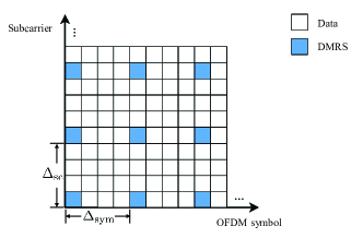
Figure 1: Illustration for reference signal placement.

The OFDM signal model is considered. The transmitted signal at the $m$-th OFDM symbol in the frequency domain is denoted as $\mathbf{x}_{m}\in\mathbb{C}^{N\times 1}$, where $N$ is the number of subcarriers. Considering a single-input single-output (SISO) channel model, the $m$-th OFDM symbol at the receiver side can be represented as

$$\mathbf{y}_{m}=\mathbf{\overline{X}}_{m}\mathbf{h}_{m}+\mathbf{w}_{m},$$

where $\mathbf{\overline{X}}_{m}=\operatorname{diag}\left(\mathbf{x}_{m}\right)$ is a diagonal matrix of the transmitted signal $\mathbf{x}_{m}$, $\mathbf{h}_{m}$ is the channel frequency response (CFR) at the $m$-th OFDM symbol to be estimated, and $\mathbf{w}_{m}\sim\mathcal{CN}(\mathbf{0},\sigma^{2}_{w}\mathbf{I}_{N})$ is the additive white Gaussian noise.

In 5G systems, channel decoding is performed in blocks, where multiple OFDM symbols in a slot are processed at the receiver for channel estimation and decoding. Assuming that there are $M$ symbols in one slot, the transmitted signal, CFR, and the received signal can be represented by $N\times M$ matrices $\bf{X}$, $\bf{H}$, and $\bf{Y}$, respectively. Mathematically, the $N\times M$ matrices can be reshaped into $NM\times 1$ column vectors to simplify the expression as

$$\mathbf{y}=\mathbf{\overline{X}}\mathbf{h}+\mathbf{w},$$

where $\mathbf{\overline{X}}\in\mathbb{C}^{MN\times MN}$ is the diagonal matrix for the vectorized $\bf{X}$, i.e., $\mathbf{\overline{X}}=\operatorname{diag}\left(\text{vec}(\mathbf{X})\right)$. For a multi-path time-varying communication channel (i.e., a doubly selective channel), the CFR at the $n$-th subcarrier and $m$-th OFDM symbol can be modeled as

$$(\mathbf{H})_{n,m}=\sum_{l=1}^{L}\alpha_{l}e^{-j2\pi n\Delta_{\mathrm{f}}\tau_{l}}e^{j2\pi mT_{\mathrm{o}}f_{\mathrm{d},l}},$$ (1)

where $L$ is the number of paths, and $\alpha_{l}$, $\tau_{l}$ and $f_{\mathrm{d},l}$ are the complex path gain, delay, and Doppler shift corresponding to the $l$-th path, $\Delta_{\mathrm{f}}$ is the subcarrier spacing, and $T_{\mathrm{o}}$ is the symbol duration including the cyclic prefix (CP). Thus, the CFR to be estimated is $\mathbf{h}=\mathrm{vec}(\mathbf{H})$.

To support channel estimation, some pilots or reference signals, called demodulation reference signals (DMRSs) in 4G and 5G systems, must be inserted into the transmitted OFDM signal. In this paper, the scattered DMRS pattern in 5G systems is considered, as shown in Fig. 1. More specifically, the pilot subcarrier interval and pilot symbol interval for DMRSs are denoted as $\Delta_{\text{sc}}$ and $\Delta_{\text{sym}}$, respectively. Thus, the number of DMRSs is $N_{\mathrm{p}}=\lceil N/\Delta_{\text{sc}}\rceil$ along the subcarrier and $M_{\mathrm{p}}=\lceil M/\Delta_{\text{sym}}\rceil$ along the symbol. For simplicity, we assume that $N/\Delta_{\text{sc}}$ and $M/\Delta_{\text{sym}}$ are integers. Let $\mathbb{P}$ and $\mathbb{Q}$ denote the sets containing the subcarrier indices and symbol indices for DMRSs, respectively. Then,

$$\mathbb{P}=\left\{p(n)|p(n)=(n-1)\Delta_{\text{sc}}+1,n=1,2,\cdots,N_{\mathrm{p}}\right\},$$

$$\mathbb{Q}=\left\{q(m)|q(m)=(m-1)\Delta_{\text{sym}}+1,m=1,2,\cdots,M_{\mathrm{p}}\right\}.$$

Concatenating all the DMRSs symbol by symbol, we can use $\mathbf{x}_{\mathrm{p}}\in\mathbb{C}^{N_{\mathrm{p}}M_{\mathrm{p}}\times 1}$ to denote the DMRSs in a vector form. The channel estimation problem is thus to solve for $\mathbf{h}\in\mathbb{C}^{NM\times 1}$ (or $\mathbf{H}\in\mathbb{C}^{N\times M}$) with given knowledge of DMRSs, $\mathbf{x}_{\mathrm{p}}$, which constitute partial diagonal entries of $\mathbf{\overline{X}}$.

II-C Signal Model for Sensing

In bistatic ISAC systems, communications and sensing share the same transmitted signal and physical channel [22], so the signal model for sensing, in general, is the same as that for communications. In radar sensing, the DMRSs are extracted for target/path detection. However, the radar coherent processing interval (CPI) is usually much longer than a communication slot. Thus, multiple slots can be combined to carry out radar signal processing, which can improve the Doppler resolution. The goal for sensing is to estimate the number of targets, the radar-cross section (RCS), distance, and relative velocity of each target, which can be inferred from channel parameters $L$, $\alpha_{l}$, $\tau_{l}$ and $f_{\mathrm{d},l}$, respectively.

III Framework Design for Sensing-Assisted Channel Estimator

In this section, the architecture of the sensing-assisted channel estimator is first developed. Then, a low-complexity sensing algorithm tailored for the estimator is provided. Finally, the procedure of leveraging sensing information to enhance channel estimation is presented.

III-A Architecture Design

Given the distinct objectives of sensing and communications, the algorithms for target sensing and channel estimation differ significantly. However, exploiting the intrinsic correlation within the channel model allows for the utilization of sensing information to enhance communication channel estimation. To this end, a sensing-assisted channel estimation architecture is proposed for bistatic ISAC systems.

As shown in Fig. 2, the received signal $\bf{y}$ after communication synchronization is fed to the communication block and the sensing block in parallel. The DMRSs are extracted for channel estimation and sensing separately. Although the received signal has been synchronized for OFDM demodulation, the synchronization error is usually unacceptable for bistatic sensing [37]. Therefore, sampling time offset (STO) and carrier frequency offset (CFO) calibrations are further required. Since STO and CFO are part of the information for communication channels, unlike usual sensing procedures, sensing-assisted communication channel estimation needs to use the sensing information before STO and CFO calibrations. Thus, the sensing block is designed with two independent subsequent subblocks: sensing algorithm and system calibration. The sensing results, including the number of targets $\hat{L}$, delay $\hat{\tau}_{l}$, Doppler shift $\hat{f}_{\mathrm{d},l}$, and complex path gain $\hat{\alpha}_{l}$ of each path $l$ before calibration, are fed into the communication block. Utilizing the above sensing results, channel estimation is expected to be more accurate, resulting in a better decoding performance. In fact, our designed algorithm does not need the complex path gain $\hat{\alpha}_{l}$ of each path, reducing the complexity of the sensing algorithm. The sensing result of $\hat{\alpha}_{l}$ in the architecture is provided to support a more general sensing-assisted channel estimation algorithm design.

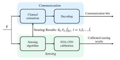
Figure 2: Architecture of sensing-assisted channel estimator.

III-B Low Complexity Sensing Algorithm Tailored for the Estimator

Commonly used sensing algorithms include periodogram-based algorithms, subspace-based algorithms (such as MUSIC and ESPRIT), and compressed-sensing-based algorithms. The subspace-based and compressed-sensing-based sensing algorithms can achieve high accuracy and super-resolution, but suffer from much higher computational complexity compared with the periodogram-based algorithms.

Since channel estimation and communication decoding are performed in real-time in 5G systems, a low-complexity sensing algorithm is preferred in the context of sensing-assisted channel estimation. Therefore, a tailored low-complexity periodogram-based algorithm is adopted as follows. The LS estimation at DMRSs is first obtained, which is given by

$$\hat{\mathbf{h}}_{\mathrm{p}}^{\mathrm{LS}}=\overline{\mathbf{X}}_{\mathrm{p}}^{-1}\mathbf{y}_{\mathrm{p}},$$ (2)

where $\overline{\mathbf{X}}_{\mathrm{p}}=\text{diag}(\mathbf{x}_{\mathrm{p}})$ is a diagonal matrix of the transmit DMRSs $\mathbf{x}_{\mathrm{p}}$, and $\mathbf{y}_{\mathrm{p}}$ is the received signal at DMRSs. The LS estimation can also be realized by element-wise operation as

$$(\hat{\mathbf{H}}^{\mathrm{LS}})_{n,m}=(\mathbf{Y})_{n,m}/(\mathbf{X})_{n,m}\quad n\in\mathbb{P},m\in\mathbb{Q}.$$

The LS estimated matrix for DMRSs can be expressed as $\hat{\mathbf{H}}^{\text{LS}}_{\mathbf{p}}=[\hat{\mathbf{h}}_{\mathrm{p},1}^{\mathrm{LS}},\hat{\mathbf{h}}_{\mathrm{p},2}^{\mathrm{LS}},\cdots,\hat{\mathbf{h}}_{\mathrm{p},M_{\mathrm{p}}}^{\mathrm{LS}}]$, where $\hat{\mathbf{h}}_{\mathrm{p},i}^{\mathrm{LS}}=[(\hat{\mathbf{H}}^{\mathrm{LS}})_{p(1),i},(\hat{\mathbf{H}}^{\mathrm{LS}})_{p(2),i},\cdots,(\hat{\mathbf{H}}^{\mathrm{LS}})_{p(N_{\mathrm{p}}),i}]^{\mathsf{T}}$. Then, two-dimensional fast Fourier transform (2D FFT) is adopted to implement the periodogram-based algorithm by conducting $M_{\text{Per}}$-point FFT along the row and $N_{\text{Per}}$-point IFFT along the column of matrix $\hat{\mathbf{H}}^{\text{LS}}_{\mathbf{p}}$ to obtain the range-Doppler (RD) map as follows [38, 39]:

$$\operatorname{Per}(n,m)$$

$$=\frac{1}{NM}\left|\sum_{k=0}^{N_{\text{Per}}-1}\left(\sum_{l=0}^{M_{\text{Per}}-1}(\mathbf{H}_{\mathrm{p}}^{\mathrm{LS}})_{k,l}e^{-j2\pi\frac{lm}{M_{\text{Per}}}}\right)e^{j2\pi\frac{kn}{N_{\text{Per}}}}\right|^{2},$$

where $\operatorname{Per}(n,m)$ denotes the element on the $n$-th row and $m$-th column of the RD map. Targets are further extracted from local peaks on the RD map. For example, if $\text{Per}(n,m)$ is detected as a local peak, the corresponding delay and Doppler are further given by

$$\tau =\frac{n}{\Delta_{\mathrm{f}}N_{\text{Per}}\Delta_{\mathrm{sc}}},$$

$$f_{\text{d}} =\frac{m}{T_{o}M_{\text{Per}}\Delta_{\mathrm{sym}}}.$$

To achieve high accuracy for sensing, the 2D FFT implementation encounters two challenges in terms of computational complexity. First, the estimation accuracy of range and velocity directly depends on the value of $N_{\text{Per}}$ and $M_{\text{Per}}$, respectively. With larger numbers of FFT points, higher estimation accuracy can be achieved, which, however, leads to higher computational complexity. Second, the above 2D FFT operation will result in many high sidelobes for each target/path. These sidelobes, especially from strong targets/paths, can obscure or interfere with the detection of weak ones. To address this problem, successive target cancellation is required, which also adds to the computational complexity.

Therefore, the above 2D FFT implementation is further tailored in two aspects to reduce complexity, supporting real-time channel estimation. First, we choose relatively small values for $N_{\text{Per}}$ and $M_{\text{Per}}$, which sacrifices the estimation accuracy. Second, windowed FFT is adopted to suppress the sidelobes so that the complexity of multi-target detection can be reduced, at the cost of degraded resolution. The LS estimated matrix after windowing can be expressed as

$$\hat{\mathbf{H}}^{\mathrm{LS},\text{win}}_{\mathrm{p}}=\mathbf{A}\odot\hat{\mathbf{H}}^{\mathrm{LS}}_{\mathrm{p}}$$

The windowing matrix can be made up of two 1D windowing vectors as

$$\mathbf{A}=\frac{1}{\|\mathbf{a}_{\mathrm{F}}\|^{2}\|\mathbf{a}_{\mathrm{T}}\|^{2}}\mathbf{a}_{\mathrm{F}}\mathbf{a}_{\mathrm{T}}^{\mathsf{T}},$$

where $\mathbf{a}_{\mathrm{F}}\in\mathbb{R}^{N_{\mathrm{p}}\times 1}$ is the frequency domain windowing vector, and $\mathbf{a}_{\mathrm{T}}\in\mathbb{R}^{M_{\mathrm{p}}\times 1}$ is the time domain windowing vector. The commonly used windows such as hanning or hamming windows can be applied. By using windows, close targets/paths may be indistinguishable and appear as a single target/path on the RD map. The suppressed sidelobes enable the signal processing to detect all close targets/paths at a time. The resolution of delay and Doppler not only depends on the window function adopted, but also on the bandwidth (for delay resolution) and number of symbols (for Doppler resolution). To improve the Doppler resolution, the sensing algorithm executed in the current slot can reuse the DMRSs in the past $S$ slots, if the total duration is within the radar CPI.

In summary, the periodogram-based sensing algorithm is applied and tailored in two aspects for sensing-assisted channel estimation to reduce the complexity: 1) a small number of FFT points is used; 2) windowed FFT is adopted for multi-path detection. The sensing results generated by the tailored algorithm may exhibit relatively large errors. Nevertheless, they can still be effectively leveraged to enhance channel estimation, achieving robust performance. This is made possible by the tolerance factors incorporated into our algorithm design, as detailed in Section IV. In addition, the complex path gain of each target/path is not required in our algorithm, which also reduces the complexity of the sensing algorithm. Otherwise, further steps are required to obtain an estimate of path gain.

III-C Sensing-Assisted Channel Estimation Procedure

As shown in the architecture in Fig. 2, the sensing results are fed into the channel estimation block to enhance its performance. In each slot, the sensing algorithm will be performed on the LS estimate of DMRSs. If the sensing results for all parameters (i.e., $\hat{L}$ and $\{\hat{\alpha}_{l},\hat{\tau}_{l},\hat{f}_{\mathrm{d},l}\}$ for each $l$) can be obtained, we can use Eq. (1) to directly calculate the CFR. This direct reconstruction of CFR is sensitive to sensing errors, i.e., it requires high sensing accuracy. To resolve this challenge, we incorporate the coarse estimated sensing results (i.e., $\{\hat{\tau}_{l},\hat{f}_{\mathrm{d},l}\}$, $l=1,2,\cdots,\hat{L}$) obtained from the tailored sensing algorithm into LMMSE channel estimation framework and design tolerance factors to combat potential sensing errors.

The LMMSE estimator is mathematically given by [40]

$$\hat{\mathbf{h}}_{\mathrm{LMMSE}} =\arg\min_{\hat{\mathbf{h}}}\left\|\mathbf{h}-\hat{\mathbf{h}}\right\|_{2}^{2}$$

$$=\mathbf{R}_{\mathbf{h}\mathbf{h}_{\mathrm{p}}}\left(\mathbf{R}_{\mathbf{h}_{\mathrm{p}}\mathbf{h}_{\mathrm{p}}}+\sigma_{w}^{2}(\mathbf{X}_{\mathrm{p}}\mathbf{X}_{\mathrm{p}}^{\mathsf{H}})^{-1}\right)^{-1}\hat{\mathbf{h}}_{\mathrm{p}}^{\mathrm{LS}},$$

where $\mathbf{R}_{\mathbf{h}\mathbf{h}_{\mathrm{p}}}=\mathbb{E}\left[\mathbf{h}\mathbf{h}_{\mathrm{p}}^{\mathsf{H}}\right]$ and $\mathbf{R}_{\mathbf{h}_{\mathrm{p}}\mathbf{h}_{\mathrm{p}}}=\mathbb{E}\left[\mathbf{h}_{\mathrm{p}}\mathbf{h}_{\mathrm{p}}^{\mathsf{H}}\right]$ are the correlation matrices of CFR and $\mathbf{h}_{\mathrm{p}}$ is the CFR at pilot signals. To avoid calculating $(\mathbf{X}_{\mathrm{p}}\mathbf{X}_{\mathrm{p}}^{\mathsf{H}})^{-1}$ in each estimation iteration, the term $\sigma^{2}_{w}(\mathbf{X}_{\mathrm{p}}\mathbf{X}_{\mathrm{p}}^{\mathsf{H}})^{-1}$ can be simplified into $\frac{\beta}{\text{SNR}}\mathbf{I}_{N_{\mathrm{p}}M_{\mathrm{p}}}$ given a specific modulation, where $\beta$ is a factor only related to the modulation constellation, and SNR is the operating SNR. If BPSK/QPSK is applied, $\beta=1$. The operating SNR is suggested to use a large value, for example, $10^{5}$, causing only ignorable loss in overall channel estimation performance [34, 27]. $\hat{\mathbf{h}}_{\mathrm{p}}^{\mathrm{LS}}$ is the real-time LS estimate of DMRSs according to Eq. (2). Therefore, the core of the proposed sensing-assisted LMMSE estimation algorithm is to leverage the sensing information to construct $\hat{\mathbf{R}}_{\mathbf{h}\mathbf{h}_{\mathrm{p}}}$ and $\hat{\mathbf{R}}_{\mathbf{h}_{\mathrm{p}}\mathbf{h}_{\mathrm{p}}}$ that approximate $\mathbf{R}_{\mathbf{h}\mathbf{h}_{\mathrm{p}}}$ and $\mathbf{R}_{\mathbf{h}_{\mathrm{p}}\mathbf{h}_{\mathrm{p}}}$.

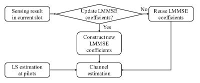
Figure 3: Sensing-assisted channel estimation procedure.

Since LMMSE by nature is a linear estimator, the estimated CFR vector can be represented as a linear combination of LS results at pilot signals, which is given by

$$\hat{\mathbf{h}}_{\mathrm{LMMSE}}=\mathbf{W}\hat{\mathbf{h}}_{\mathrm{p}}^{\mathrm{LS}},$$

where $\mathbf{W}=\hat{\mathbf{R}}_{\mathbf{h}\mathbf{h}_{\mathrm{p}}}\left(\hat{\mathbf{R}}_{\mathbf{h}_{\mathrm{p}}\mathbf{h}_{\mathrm{p}}}+\frac{\beta}{\text{SNR}}\mathbf{I}_{N_{\mathrm{p}}M_{\mathrm{p}}}\right)^{-1},$ is defined as the LMMSE coefficients. The update of $\mathbf{W}$ requires matrix inversion, which leads to high computational complexity. Therefore, it is not preferable for $\mathbf{W}$ to be updated frequently, and an update check for the LMMSE coefficients is designed in our sensing-assisted LMMSE channel estimation algorithm to avoid frequent updates.

The overall procedure of our proposed channel estimation algorithm is shown in Fig. 3. In each slot, the sensing algorithm will feed the coarse sensing results to the channel estimation block. The update check module will determine whether to update the LMMSE coefficients or not. If yes, $\hat{\mathbf{R}}_{\mathbf{h}\mathbf{h}_{\mathrm{p}}}$ and $\hat{\mathbf{R}}_{\mathbf{h}_{\mathrm{p}}\mathbf{h}_{\mathrm{p}}}$ will be updated with sensing results in the current slot. Otherwise, the LMMSE coefficients from the last slot can still be used. Finally, the CFR can be estimated by multiplying the LMMSE channel coefficient matrix by the LS result from the current slot. The ability to tolerate sensing errors and the lowered update frequency is enabled by the tolerance factors incorporated into our algorithm design, as discussed in the next section.

IV Sensing-Assisted LMMSE Algorithm

In this section, we will elaborate on the operation logic of the sensing-assisted LMMSE channel estimation algorithm. The construction of channel correlation matrices with sensing results is first presented. The determination of tolerance factors is then designed, followed by the update scheme of LMMSE coefficients.

IV-A Construction of Correlation Matrices

For LMMSE estimation, the calculation of channel correlation matrices can be decomposed into time-domain and frequency-domain correlation matrices [41], i.e., $\mathbf{R}_{\mathbf{h}\mathbf{h}_{\mathrm{p}}}=\mathbf{R}_{\mathrm{T},\mathbf{h}\mathbf{h}_{\mathrm{p}}}\otimes\mathbf{R}_{\mathrm{F},\mathbf{h}\mathbf{h}_{\mathrm{p}}}$ and $\mathbf{R}_{\mathbf{h}_{\mathrm{p}}\mathbf{h}_{\mathrm{p}}}=\mathbf{R}_{\mathrm{T},\mathbf{h}_{\mathrm{p}}\mathbf{h}_{\mathrm{p}}}\otimes\mathbf{R}_{\mathrm{F},\mathbf{h}_{\mathrm{p}}\mathbf{h}_{\mathrm{p}}}$. Analogous to the idea of time-frequency separability, for the constructed correlation matrices, $\hat{\mathbf{R}}_{\mathbf{h}\mathbf{h}_{\mathrm{p}}}\in\mathbb{C}^{NM\times N_{\mathrm{p}}M_{\mathrm{p}}}$ and $\hat{\mathbf{R}}_{\mathbf{h}_{\mathrm{p}}\mathbf{h}_{\mathrm{p}}}\in\mathbb{C}^{N_{\mathrm{p}}M_{\mathrm{p}}\times N_{\mathrm{p}}M_{\mathrm{p}}}$, we can approach them from time domain and frequency domain separately, i.e.,

$$\hat{\mathbf{R}}_{\mathbf{h}\mathbf{h}_{\mathrm{p}}}=\hat{\mathbf{R}}_{\mathrm{T},\mathbf{h}\mathbf{h}_{\mathrm{p}}}\otimes\hat{\mathbf{R}}_{\mathrm{F},\mathbf{h}\mathbf{h}_{\mathrm{p}}},$$ (3)

$$\hat{\mathbf{R}}_{\mathbf{h}_{\mathrm{p}}\mathbf{h}_{\mathrm{p}}}=\hat{\mathbf{R}}_{\mathrm{T},\mathbf{h}_{\mathrm{p}}\mathbf{h}_{\mathrm{p}}}\otimes\hat{\mathbf{R}}_{\mathrm{F},\mathbf{h}_{\mathrm{p}}\mathbf{h}_{\mathrm{p}}}.$$ (4)

The time-domain and frequency-domain channel correlation matrices can be constructed with sensing results. We can directly calculate the correlation matrices if perfect sensing results of channel parameters can be obtained. However, sensing errors always exist, especially when a low-complexity sensing algorithm is applied. To handle sensing errors, tolerance factors are introduced in our algorithm to construct the channel correlation matrices. More specifically, we design a delay distribution function $f_{\bm{\tau}}(\tau)$ and a Doppler distribution function $f_{\bm{f_{\mathrm{d}}}}(f_{\mathrm{d}})$ to calculate the channel correlation matrices in a closed-form.

The delay distribution function is designed using the estimated delays $\hat{\tau}_{l}\text{, }l=1,2,\cdots,\hat{L}$ as follows. Considering the sensing error, we assume that the actual delay for the $l$-th path uniformly lies within $\hat{\tau_{l}}\pm\frac{1}{2}C_{\mathrm{F},l}$, where $C_{\mathrm{F},l}$ is the designed frequency-domain tolerance factor to accommodate sensing imperfection for each path. The delay distribution function is designed as

$$f_{\bm{\tau}}(\tau)=\left\{\begin{array}[]{ll}1/C_{\mathrm{F},l},&\text{ if }\tau\in[\hat{\tau}_{l}-\frac{C_{\mathrm{F},l}}{2},\hat{\tau}_{l}+\frac{C_{\mathrm{F},l}}{2}]\\ &\hfill{l=1,2,\cdots,\hat{L}}\\ 0,&\text{ otherwise }\end{array}.\right.$$ (5)

In the next subsection, we will explain why the assumption of uniform distribution is reasonable. With the above delay distribution function, the frequency-domain correlation matrices $\hat{\mathbf{R}}_{\mathrm{F},\mathbf{h}\mathbf{h}_{\mathrm{p}}}\in\mathbb{C}^{N\times N_{\mathrm{p}}}$ and $\hat{\mathbf{R}}_{\mathrm{F},\mathbf{h}_{\mathrm{p}}\mathbf{h}_{\mathrm{p}}}\in\mathbb{C}^{N_{\mathrm{p}}\times N_{\mathrm{p}}}$ can be obtained with a closed-from expression for each entry. More specifically, the $(m,n)$th entry can be calculated in the following way,

$$(\hat{\mathbf{R}}_{\text{F},\mathbf{h}\mathbf{h}_{\mathrm{p}}})_{m,n}=r_{\text{F}}(m-p(n)),$$

$$(\hat{\mathbf{R}}_{\text{F},\mathbf{h}_{\mathrm{p}}\mathbf{h}_{\mathrm{p}}})_{m,n}=r_{\text{F}}(p(m)-p(n)),$$

where $r_{\text{F}}(k)$ is given by

$$r_{\text{F}}(k) =\!\int\!\!\cdots\!\!\int\prod_{l=1}^{\hat{L}}f_{\bm{\tau}}(\tau)\left[\sum_{l=1}^{\hat{L}}\theta\left(\tau_{l}\right)e^{-j2\pi\tau_{l}k\Delta_{\mathrm{f}}}\right]\!\!\cdot\!d\tau_{1}\cdots d\tau_{\hat{L}}$$

$$=\!\sum_{l=1}^{\hat{L}}\int f_{\bm{\tau}}(\tau)\theta\left(\tau_{l}\right)e^{-j2\pi\tau_{l}k\Delta_{\mathrm{f}}}d\tau_{l}.$$

Using Eq. (5), if the multi-path intensity profile is set as a constant, i.e., $\theta(\tau_{l})=1$ for $l=1,2,\cdots\hat{L}$, the closed-form expression for entries after normalization is given by

$$r_{\mathrm{F}}(k) =\!\left\{\!\!\begin{array}[]{ll}\frac{1}{\hat{L}}\sum_{l}\frac{1}{C_{\mathrm{F},l}}\frac{e^{-j2\pi k\Delta_{\text{f}}(\hat{\tau}_{l}+\frac{C_{\mathrm{F},l}}{2})}\left(1-e^{j2\pi k\Delta_{\text{f}}C_{\mathrm{F},l}}\right)}{-j2\pi k\Delta_{\text{f}}},&\!\!\!k\neq 0\\ 1,&\!\!\!k=0\end{array}\right.$$

$$=\frac{1}{\hat{L}}\sum_{l}\text{sinc}(k\Delta_{\text{f}}C_{\mathrm{F},l})e^{-j2\pi k\Delta_{\text{f}}\hat{\tau}_{l}}.$$

Theoretically, $\theta(\tau_{l})$ should be assigned with the path gain of each path $l$. However, the estimation of path gains can cause additional complexity. Moreover, our simulations show that the selection of the multi-path intensity profile has little impact on the LMMSE performance. Therefore, we adopt a constant multi-path intensity profile.

Similarly, the Doppler distribution function is designed using the Doppler estimates $\hat{f}_{\mathrm{d},l}$, $l=1,2,\cdots,\hat{L}$. Assuming that the Doppler shift for the $l$-th path uniformly lies within $\hat{f}_{\mathrm{d},l}\pm\frac{1}{2}C_{\mathrm{T},l}$, where $C_{\mathrm{T},l}$ is the designed time-domain tolerance factor, the distribution function of Doppler shift is

$$f_{\bm{f_{\mathrm{d}}}}(f_{\mathrm{d}})=\left\{\begin{array}[]{ll}1/C_{\mathrm{T},l},&\text{ if }f_{\mathrm{d}}\in[\hat{f}_{\mathrm{d},l}-\frac{C_{\mathrm{T},l}}{2},\hat{f}_{\mathrm{d},l}+\frac{C_{\mathrm{T},l}}{2}]\\ &\hfill{l=1,2,\cdots,\hat{L}}\\ 0,&\text{ otherwise }\end{array}.\right.$$ (6)

Therefore, the closed-form expression for each entry of the constructed time-domain correlation matrices $\hat{\mathbf{R}}_{\mathrm{T},\mathbf{h}\mathbf{h}_{\mathrm{p}}}\in\mathbb{C}^{M\times M_{\mathrm{p}}}$ and $\hat{\mathbf{R}}_{\mathrm{T},\mathbf{h}_{\mathrm{p}}\mathbf{h}_{\mathrm{p}}}\in\mathbb{C}^{M_{\mathrm{p}}\times M_{\mathrm{p}}}$ is given by

$$(\hat{\mathbf{R}}_{\text{T},\mathbf{h}\mathbf{h}_{\mathrm{p}}})_{m,n}=r_{\text{T}}(m-q(n)),$$

$$(\hat{\mathbf{R}}_{\text{T},\mathbf{h}_{\mathrm{p}}\mathbf{h}_{\mathrm{p}}})_{m,n}=r_{\text{T}}(q(m)-q(n)),$$

where

$$r_{\mathrm{T}}(k) =\!\left\{\!\!\begin{array}[]{ll}\!\!\frac{1}{\hat{L}}\sum_{l}\frac{1}{C_{\mathrm{T},l}}\frac{e^{j2\pi kT_{\mathrm{o}}(\hat{f}_{\mathrm{d},l}+\frac{C_{\mathrm{T},l}}{2})}\left[1-e^{-j2\pi kT_{\mathrm{o}}C_{\mathrm{T},l}}\right]}{j2\pi kT_{\mathrm{o}}},&\!\!\!\!\!k\neq 0\\ \!\!1,&\!\!\!\!\!k=0\end{array}\right.$$

$$=\frac{1}{\hat{L}}\sum_{l}\text{sinc}(kT_{\mathrm{o}}C_{\mathrm{T},l})e^{j2\pi kT_{\mathrm{o}}\hat{f}_{\mathrm{d},l}}.$$

The proposed sensing-assisted LMMSE algorithm can tolerate sensing errors by $\pm\frac{1}{2}C_{\mathrm{F},l}$ and $\pm\frac{1}{2}C_{\mathrm{T},l}$ in the frequency domain and time domain, respectively. The choice of tolerance factors can directly impact the accuracy of channel estimation. Small tolerance factors may fail to account for sensing errors, significantly degrading estimation performance. On the other hand, excessively large tolerance factors can also deteriorate performance. As a result, the tolerance factors should be properly designed.

IV-B Determination of Tolerance Factors

The frequency-domain and time-domain tolerance factors are introduced to tolerate the deviations between the estimated delays and Doppler shifts and the true ones in the construction of correlation matrices. The goal is thus to guarantee that the actual delay and Doppler of the $l$-th path lie within $\hat{\tau_{l}}\pm\frac{1}{2}C_{\mathrm{F},l}$ and $\hat{f}_{\mathrm{d},l}\pm\frac{1}{2}C_{\mathrm{T},l}$, respectively. To achieve this goal, the sensing error caused by the adopted sensing algorithm should be first considered.

There are always sensing errors in wireless sensing. For an unbiased sensing estimator, the estimation accuracies of the delay and Doppler are theoretically lower bounded by their Cramér–Rao lower bounds (CRLB), which can be asymptotically approached by a maximum likelihood (ML) estimator. Given the OFDM radar sensing, the variances of delay and Doppler shift estimates are lower bounded by the averaged CRLBs [39]

$$var(\hat{\tau})\geq\frac{6\sigma_{w}^{2}}{(N_{\text{p}}^{2}-1)N_{\text{p}}M_{\text{p}}}\left(\frac{1}{2\pi\Delta_{\text{sc}}\Delta_{\mathrm{f}}}\right)^{2},$$

$$var(\hat{f}_{\mathrm{d}})\geq\frac{6\sigma_{w}^{2}}{(M_{\text{p}}^{2}-1)N_{\text{p}}M_{\text{p}}}\left(\frac{1}{2\pi\Delta_{\text{sym}}T_{\mathrm{o}}}\right)^{2}.$$

The periodogram-based sensing algorithm is an unbiased estimator, which can approach the CRLB in the high SNR regime [42][43]. In this paper, a windowed 2D FFT algorithm is applied to implement the periodogram-based sensing algorithm. If the delays and Doppler shifts to be estimated are located exactly on the FFT bins, i.e., the estimation is on-grid, the mean squared estimation error can approach the CRLB. However, off-grid estimation can always be the case and thus quantization errors can be the source of sensing errors, which will not exceed one half of the FFT bin widths. The bin widths for delay estimation and Doppler estimation are given by

$$\tau_{\text{bin}}=\frac{1}{\Delta_{\mathrm{f}}N_{\text{Per}}\Delta_{\mathrm{sc}}},$$

$$f_{\text{d,bin}}=\frac{1}{T_{\mathrm{o}}M_{\text{Per}}\Delta_{\mathrm{sym}}}.$$

Since the value of CRLB is much smaller than the bin width, especially when a small number of FFT points is used, the estimation error is dominated by the quantization error. If we assume that the delay and Doppler are uniformly distributed over the estimation range, the sensing error can be treated as uniformly distributed within a sensing bin. In other words, given the sensing results of $\hat{\tau}$ and $\hat{f}_{\text{d}}$ on the FFT bins, the delay and Doppler can be assumed to be uniformly distributed in $[-\frac{\tau_{\text{bin}}}{2}+\hat{\tau},\frac{\tau_{\text{bin}}}{2}+\hat{\tau}]$ and $[-\frac{f_{\text{d,bin}}}{2}+\hat{f}_{\text{b}},\frac{f_{\text{d,bin}}}{2}+\hat{f}_{\text{b}}]$, respectively. As a result, the tolerance factors should be designed at least larger than the FFT bin width, so that sensing errors can be tolerated.

In our tailored sensing algorithm, a window is used and thus all targets can be detected once on the RD map. When two targets/paths are within the resolution, they will become irresolvable, resulting in sensing errors larger than the FFT bin width. The sensing error should instead take into consideration the delay and Doppler resolution. According to [44], the resolution of the windowed DFT is determined by the 6-dB bandwidth, which can be calculated by the fundamental resolution multiplied by a fixed factor. The factor only depends on the type of window function. If a 2D Hamming window is assumed and $S$ slots are used for sensing, the resolution for delay and Doppler can be represented by

$$\tau_{\text{resol}}=\frac{1.81}{N\Delta_{\mathrm{f}}},$$

$$f_{\text{d,resol}}=\frac{1.81}{SMT_{\mathrm{o}}},$$

where 1.81 is the factor for the Hamming window. Without any prior knowledge about the target distribution, we can also assume that the sensing error caused by the resolution problem is uniformly distributed.

For each peak detected on the RD map, if no action is further taken to distinguish whether it belongs to the single-target case or multi-target case, the tolerance factors for all target/paths can be set equal to the resolution, i.e., $C_{\mathrm{F},l}=\tau_{\text{resol}}$ and $C_{\mathrm{T},l}=f_{\text{d,resol}}$ for all $l$s. Otherwise, we can assign the bin width to tolerance factors in the single-target case and the resolution to tolerance factors in the multi-target case.

IV-C Update of LMMSE Coefficients

Since the communication channel varies over time when the doubly-selective channel model is considered, the channel correlation matrices or LMMSE coefficients should be updated if the channel parameters are changed. An update check for the LMMSE coefficients is designed. The estimator always keeps a record of the adopted delay distribution set $\mathbb{S}_{\tau}$ and Doppler distribution set $\mathbb{S}_{f_{\mathrm{d}}}$ from the latest update. The sensing results obtained in the current slot are inputs for the update check, and the update is triggered if one of the following conditions is satisfied: 1) $\tau_{l}\notin\mathbb{S}_{\tau},\forall l$; 2)$f_{\mathrm{d},l}\notin\mathbb{S}_{f_{\mathrm{d}}},\forall l$.

V Performance Analysis

In this section, the performance of the proposed sensing-assisted LMMSE channel estimator in terms of NMSE and computational complexity is analyzed.

V-A NMSE Analysis

NMSE is widely used to characterize the performance of a channel estimator, which is given by

$$\text{NMSE}=\frac{1}{NM}\text{Trace}(\mathbf{M}),$$ (7)

where $\mathbf{M}$ is the MSE matrix calculated by

$$\mathbf{M}=\mathbb{E}\left[(\mathbf{h}-\hat{\mathbf{h}})(\mathbf{h}-\hat{\mathbf{h}})^{\mathsf{H}}\right].$$

In the proposed sensing-assisted LMMSE channel estimation, the channel estimator is

$$\hat{\mathbf{h}}=\hat{\mathbf{R}}_{\mathbf{h}\mathbf{h}_{\mathrm{p}}}\left(\hat{\mathbf{R}}_{\mathbf{h}_{\mathrm{p}}\mathbf{h}_{\mathrm{p}}}+\hat{\sigma}_{w}^{2}\mathbf{I}_{N_{\mathrm{p}}M_{\mathrm{p}}}\right)^{-1}\hat{\mathbf{h}}_{\mathrm{p}}^{\mathrm{LS}},$$

where BPSK/QPSK modulation is used for the DMRS and $\hat{\sigma}_{w}^{2}=\frac{1}{\text{SNR}}$ is defined. The MSE matrix of our proposed method can be further expressed as

$$\mathbf{M}=\mathbf{R}_{\mathbf{h}\mathbf{h}}\!\!-\!\!\mathbf{R}_{\mathbf{h}\mathbf{h}_{\mathrm{p}}}\mathbf{W}^{\mathsf{H}}\!\!-\!\!\mathbf{W}\mathbf{R}_{\mathbf{h}_{\mathrm{p}}\mathbf{h}}\!\!+\!\!\mathbf{W}(\mathbf{R}_{\mathbf{h}_{\mathrm{p}}\mathbf{h}_{\mathrm{p}}}\!\!+\!\!\sigma_{w}^{2}\mathbf{I})\mathbf{W}^{\mathsf{H}},$$

where $\mathbf{W}=\hat{\mathbf{R}}_{\mathbf{h}\mathbf{h}_{\mathrm{p}}}\left(\hat{\mathbf{R}}_{\mathbf{h}_{\mathrm{p}}\mathbf{h}_{\mathrm{p}}}+\hat{\sigma}_{w}^{2}\mathbf{I}_{N_{\mathrm{p}}M_{\mathrm{p}}}\right)^{-1}$. In general, the performance of the channel estimation depends on the approximates of the estimated channel correlation matrices $\hat{\mathbf{R}}_{\mathbf{h}\mathbf{h}_{\mathrm{p}}}$, $\hat{\mathbf{R}}_{\mathbf{h}_{\mathrm{p}}\mathbf{h}_{\mathrm{p}}}$ and noise variance $\hat{\sigma}_{w}^{2}$ to the true channel correlation matrices $\mathbf{R}_{\mathbf{h}\mathbf{h}_{\mathrm{p}}}$, $\mathbf{R}_{\mathbf{h}_{\mathrm{p}}\mathbf{h}_{\mathrm{p}}}$ and noise variance $\sigma_{w}^{2}$. However, it is intractable to find the exact relationship between them with a closed-form expression.

Since $\mathbf{R}_{\mathbf{h}\mathbf{h}_{\mathrm{p}}}$ is not a squared matrix, it is hard to analyze the NMSE for an arbitrary estimated $\hat{\mathbf{R}}_{\mathbf{h}\mathbf{h}_{\mathrm{p}}}$. However, we can analyze the NMSE of all DMRSs, which will give the same insight into the design of tolerance factors in our proposed sensing-assisted LMMSE channel estimator. The MSE matrix for DMRSs can be expressed as

$$\mathbf{M}_{\mathrm{p}} =\!\mathbf{R}_{\mathbf{h}_{\mathrm{p}}\mathbf{h}_{\mathrm{p}}}\!\!-\!\!\mathbf{R}_{\mathbf{h}_{\mathrm{p}}\mathbf{h}_{\mathrm{p}}}\mathbf{W}_{\mathrm{p}}^{\mathsf{H}}\!\!-\!\!\mathbf{W}_{\mathrm{p}}\mathbf{R}_{\mathbf{h}_{\mathrm{p}}\mathbf{h}_{\mathrm{p}}}\!\!+\!\!\mathbf{W}_{\mathrm{p}}(\mathbf{R}_{\mathbf{h}_{\mathrm{p}}\mathbf{h}_{\mathrm{p}}}\!\!+\!\!\sigma_{w}^{2}\mathbf{I})\mathbf{W}_{\mathrm{p}}^{\mathsf{H}}\!,$$

$$=\!(\mathbf{I}_{N_{\mathrm{p}}M_{\mathrm{p}}}-\mathbf{W}_{\mathrm{p}})\mathbf{R}_{\mathbf{h}_{\mathrm{p}}\mathbf{h}_{\mathrm{p}}}(\mathbf{I}_{N_{\mathrm{p}}M_{\mathrm{p}}}-\mathbf{W}_{\mathrm{p}}^{\mathsf{H}})+\sigma_{w}^{2}\mathbf{W}_{\mathrm{p}}\mathbf{W}_{\mathrm{p}}^{\mathsf{H}},$$

where $\mathbf{W}_{\mathrm{p}}=\hat{\mathbf{R}}_{\mathbf{h}_{\mathrm{p}}\mathbf{h}_{\mathrm{p}}}\left(\hat{\mathbf{R}}_{\mathbf{h}_{\mathrm{p}}\mathbf{h}_{\mathrm{p}}}+\hat{\sigma}_{w}^{2}\mathbf{I}_{N_{\mathrm{p}}M_{\mathrm{p}}}\right)^{-1}$ is the LMMSE coefficients for DMRSs. The following Theorem gives the NMSE for the channel estimator at DMRSs.

Theorem 1.

The NMSE of our sensing-assisted LMMSE channel estimator at DMRSs is given by

$$\mathrm{NMSE}_{\mathrm{p}}=\frac{1}{N_{\mathrm{p}}M_{\mathrm{p}}}\left[\Sigma_{i=1}^{N_{\mathrm{p}}M_{\mathrm{p}}}\left((1-\lambda_{i})^{2}b_{i}+\sigma_{w}^{2}\lambda_{i}^{2}\right)\right],$$ (8)

where $\lambda_{i}=\gamma_{i}/(\gamma_{i}+\hat{\sigma}_{w}^{2})$ , $\gamma_{i}$ is a singular value of $\hat{\mathbf{R}}_{\mathbf{h}_{\mathrm{p}}\mathbf{h}_{\mathrm{p}}}=\mathbf{V}\mathbf{\Gamma}\mathbf{V}^{\mathsf{H}}$, and $b_{i}$ is a diagonal element from matrix $\mathbf{B}=\mathbf{V}^{\mathsf{H}}\mathbf{R}_{\mathbf{h}_{\mathrm{p}}\mathbf{h}_{\mathrm{p}}}\mathbf{V}$, i.e., $b_{i}=(\mathbf{B})_{i,i}$. $\mathbf{V}$ is an unitary matrix, and $\mathbf{\Gamma}$ is a diagonal matrix containing singular values $\gamma_{1}\geq\gamma_{2}\geq\cdots\geq\gamma_{N_{\mathrm{p}}M_{\mathrm{p}}}$.

Proof.

The proof can be found in Appendix A. ∎

When the constructed channel correlation matrix is the exact channel correlation matrix, i.e., $\hat{\mathbf{R}}_{\mathbf{h}_{\mathrm{p}}\mathbf{h}_{\mathrm{p}}}=\mathbf{R}_{\mathbf{h}_{\mathrm{p}}\mathbf{h}_{\mathrm{p}}}$, the lower bound for $\text{NMSE}_{\mathrm{p}}$ is given by [45]

$$\text{NMSE}_{\mathrm{p}}^{\text{lb}}\!\!\!=\!\!\frac{1}{N_{\mathrm{p}}M_{\mathrm{p}}}\left[\Sigma_{i=1}^{N_{\mathrm{p}}M_{\mathrm{p}}}\left((1-\lambda_{i})^{2}\mu_{i}+\sigma_{w}^{2}\lambda_{i}^{2}\right)\right],$$ (9)

where $\mu_{i}$ is a singular value of ${\mathbf{R}}_{\mathbf{h}_{\mathrm{p}}\mathbf{h}_{\mathrm{p}}}=\mathbf{U}\mathbf{\Sigma}\mathbf{U}^{\mathsf{H}}$. The $\text{NMSE}_{\mathrm{p}}^{\text{lb}}$ is the best NMSE performance that an LMMSE estimator can achieve. By comparing the two NMSE expressions in Eq. (8) and Eq. (9), the key distinction lies in the replacement of $\mu_{i}$ with $b_{i}$. Since $\mu_{i}$ is a singular value while $b_{i}$ is a diagonal element from the matrix $\mathbf{B}$, it is also intractable to get a closed-form relationship between $\mu_{i}$ and $b_{i}$ for the analysis.

To analyze the effect of $b_{i}$ on the NMSE, a deterministic channel is used, and thus the channel correlation matrix $\mathbf{R}_{\mathbf{h}_{\mathrm{p}}\mathbf{h}_{\mathrm{p}}}$ is of rank one. If we perform singular value decomposition (SVD) as $\mathbf{R}_{\mathbf{h}_{\mathrm{p}}\mathbf{h}_{\mathrm{p}}}=\mathbf{U}\mathbf{\Sigma}\mathbf{U}^{\mathsf{H}}$, where $\mathbf{\Sigma}$ contains singular values $\mu_{1}\geq\mu_{2}\geq\cdots\geq\mu_{N_{\mathrm{p}}M_{\mathrm{p}}}$ at its diagonals, only $\mu_{1}$ is significant. According to Theorem 1, $\text{NMSE}_{\mathrm{p}}$ can be separated into two terms, $\frac{1}{N_{\mathrm{p}}M_{\mathrm{p}}}\Sigma_{i=1}^{N_{\mathrm{p}}M_{\mathrm{p}}}(1-\lambda_{i})^{2}b_{i}$ and $\frac{1}{N_{\mathrm{p}}M_{\mathrm{p}}}\Sigma_{i=1}^{N_{\mathrm{p}}M_{\mathrm{p}}}\sigma_{w}^{2}\lambda_{i}^{2}$. Compared with the given lower bound, and the first term matters, we can thus zoom in to examine the behavior of $\Sigma_{i=1}^{N_{\mathrm{p}}M_{\mathrm{p}}}(1-\lambda_{i})^{2}b_{i}$, which is the sum of the product of $(1-\lambda_{i})^{2}$ and $b_{i}$.

The former term $(1-\lambda_{i})^{2}$ is related to the design of the approximated noise variance $\hat{\sigma}_{w}^{2}$. The sparsity of the communication channel results in a limited number of significant singular values among $\gamma_{i}$’s. $\hat{\sigma}_{w}^{2}$ further determines the number of significant singular values among $\lambda_{i}$’s by $\lambda_{i}=\gamma_{i}/(\gamma_{i}+\hat{\sigma}_{w}^{2})$. As a result, the sequence $(1-\lambda_{1})^{2}\leq(1-\lambda_{2})^{2}\leq\cdots\leq(1-\lambda_{N_{\mathrm{p}}M_{\mathrm{p}}})^{2}$ has first several (say $k_{1}$) terms insignificant, approximating zero, and other terms significant.

The latter term $b_{i}$ depends on the similarity between the actual and constructed channel covariance matrix $\mathbf{R}_{\mathbf{h}_{\mathrm{p}}\mathbf{h}_{\mathrm{p}}}$ and $\hat{\mathbf{R}}_{\mathbf{h}_{\mathrm{p}}\mathbf{h}_{\mathrm{p}}}$. Denote $\mathbf{D}=\mathbf{V}^{\mathsf{H}}\mathbf{U}$, $b_{i}$ can be further expressed as

$$b_{i}=\mu_{1}|(\mathbf{D})_{i,1}|^{2}.$$

Assume that $\mathbf{v}_{i}$ and $\mathbf{u}_{i}$ are the $i$-th column vectors of unitary matrices $\mathbf{V}$ and $\mathbf{U}$, $(\mathbf{D})_{i,1}=\mathbf{v}_{i}^{\mathsf{H}}\mathbf{u}_{1}$ shows the formulation of $(\mathbf{D})_{i,1}$. Mathematically, $|(\mathbf{D})_{i,1}|$ is the magnitude of the projection of $\mathbf{v}_{i}$ on $\mathbf{u}_{1}$, indicating the similarity of directions between the singular vectors obtained from $\mathbf{R}_{\mathbf{h}_{\mathrm{p}}\mathbf{h}_{\mathrm{p}}}$ and $\hat{\mathbf{R}}_{\mathbf{h}_{\mathrm{p}}\mathbf{h}_{\mathrm{p}}}$. Since $\hat{\mathbf{R}}_{\mathbf{h}_{\mathrm{p}}\mathbf{h}_{\mathrm{p}}}$ is constructed based on the estimated channel parameters, ideally, only the first few columns of $\mathbf{V}$ will provide close directions compared with $\mathbf{u}_{1}$. The sequence $b_{1}\geq b_{2}\geq\cdots\geq b_{N_{\mathrm{p}}M_{\mathrm{p}}}$ has first a few (say $k_{2}$) terms significant, with other terms approximating zero. The sequence also has the following property: $\sum_{i=1}^{N_{\mathrm{p}}M_{\mathrm{p}}}b_{i}=\mu_{1}$.

To reduce $\text{NMSE}_{\mathrm{p}}$, a large $k_{1}$ and a small $k_{2}$ is desired. A large $k_{1}$ can be realized by a properly selected $\hat{\sigma}_{w}^{2}$, which is consistent with the suggestion of using a large SNR in the LMMSE estimator [34, 27]. Meanwhile, well-designed tolerance factors can concentrate the energy of sequence $\{b_{i}\}$ in the first few terms. Numerically, for a one-path scenario, if the tolerance factors precisely cover the sensing error, $b_{1}$ contains over $97\%$ of the total energy. When the tolerance factors increase, the energy that $b_{1}$ contains slowly decreases. However, if the error exceeds the tolerance, the energy of $b_{1}$ can dramatically decrease. More numerical results are presented in Section VI-A.

V-B Computational Complexity Analysis

The computational complexity of our proposed sensing-assisted channel estimator stems from two components: the sensing process and the LMMSE estimation, which will be analyzed separately in the following discussion. The LS estimation for DMRSs requires $N_{\mathrm{p}}M_{\mathrm{p}}$ multiplications, which will be used for both sensing and channel estimation.

V-B1 Complexity of the Tailored Periodogram-Based Sensing Algorithm

The key operation in the tailored periodogram-based sensing algorithm is 2D FFT. Applying 2D FFT on the $N_{\mathrm{p}}\times M_{\mathrm{p}}$ LS estimate matrix is of complexity $O(N_{\text{Per}}M_{\text{Per}}\text{log}(N_{\text{Per}}M_{\text{Per}}))$. Windowed 2D FFT requires additional $N_{\mathrm{p}}\times M_{\mathrm{p}}$ element-wise multiplication before 2D FFT, while getting rid of the process of successive target cancellation that performs 2D FFT multiple times. The computational complexity of the sensing process greatly depends on the 2D FFT size, i.e., $N_{\text{Per}}$ and $M_{\text{Per}}$.

V-B2 Complexity of LMMSE Channel Estimation

The proposed LMMSE channel estimator is a 2D estimator and interpolator, obtaining the CFR for one slot at a time. As suggested by [46], the 2D LMMSE estimator and interpolator can be implemented with two 1D filters, reducing the dimension of matrices while maintaining the effectiveness of channel estimation. If the estimation and interpolation are first conducted along the OFDM symbols for $N_{p}$ subcarriers, the estimated CFR for the $n$-th subcarrier ($n\in\mathbb{P}$) is given by

$$(\hat{\mathbf{H}}^{\text{tmp}})_{n,:}\!\!=\!\!\hat{\mathbf{R}}_{\mathrm{T},\mathbf{h}\mathbf{h}_{\mathrm{p}}}\left(\hat{\mathbf{R}}_{\mathrm{T},\mathbf{h}_{\mathrm{p}}\mathbf{h}_{\mathrm{p}}}+\hat{\sigma}_{w}^{2}I_{M_{\mathrm{p}}}\right)^{-1}\!\!\begin{pmatrix}(\hat{\mathbf{H}})_{n,q(1)}\\ (\hat{\mathbf{H}}_{\mathrm{LS}})_{n,q(2)}\\ \vdots\\ (\hat{\mathbf{H}}_{\mathrm{LS}})_{n,q(M_{\mathrm{p}})}\end{pmatrix}\!\!,$$

We can denote $\mathbf{W}_{\mathrm{T}}=\hat{\mathbf{R}}_{\mathrm{T},\mathbf{h}\mathbf{h}_{\mathrm{p}}}\left(\hat{\mathbf{R}}_{\mathrm{T},\mathbf{h}_{\mathrm{p}}\mathbf{h}_{\mathrm{p}}}+\hat{\sigma}_{w}^{2}I_{M_{\mathrm{p}}}\right)^{-1}$ as the LMMSE coefficient matrix for symbol interpolation.

After that, the estimation and interpolation along the subcarriers for all $M$ symbols are conducted. The estimated CFR for the $m$-th OFDM symbol ($m=1,2,\cdots,M$) is given by

$$(\hat{\mathbf{H}})_{:,m}\!\!=\!\!\hat{\mathbf{R}}_{\mathrm{F},\mathbf{h}\mathbf{h}_{\mathrm{p}}}\left(\hat{\mathbf{R}}_{\mathrm{F},\mathbf{h}_{\mathrm{p}}\mathbf{h}_{\mathrm{p}}}+\hat{\sigma}_{w}^{2}I_{N_{\mathrm{p}}}\right)^{-1}\!\!\begin{pmatrix}(\hat{\mathbf{H}}^{\text{tmp}})_{p(1),m}\\ (\hat{\mathbf{H}}^{\text{tmp}})_{p(2),m}\\ \vdots\\ \!(\hat{\mathbf{H}}^{\text{tmp}})_{p(N_{\mathrm{p}}),m}\end{pmatrix}\!\!.$$

$\mathbf{W}_{\mathrm{F}}=\hat{\mathbf{R}}_{\mathrm{F},\mathbf{h}\mathbf{h}_{\mathrm{p}}}\left(\hat{\mathbf{R}}_{\mathrm{F},\mathbf{h}_{\mathrm{p}}\mathbf{h}_{\mathrm{p}}}+\hat{\sigma}_{w}^{2}I_{N_{\mathrm{p}}}\right)^{-1}$ can be denoted as the LMMSE coefficient matrix for subcarrier interpolation.

For each LMMSE coefficient matrix, a matrix inversion and a matrix multiplication are required. Then, the matrix multiplication of the LMMSE coefficient matrix and the LS vector is required. If directly implementing 2D LMMSE, the operation of matrix inversion is of complexity $O(N_{\mathrm{p}}^{3}M_{\mathrm{p}}^{3})$, while additional $NMN_{\mathrm{p}}^{2}M_{\mathrm{p}}^{2}+NMN_{\mathrm{p}}M_{\mathrm{p}}$ complex multiplications are required for matrix multiplication. Assume that the adopted matrix inversion algorithm requires $kN_{\mathrm{p}}^{3}M_{\mathrm{p}}^{3}$ complex multiplications, where $k$ is a constant, then the 2D filter will result in a total of $kN_{\mathrm{p}}^{3}M_{\mathrm{p}}^{3}+NMN_{\mathrm{p}}^{2}M_{\mathrm{p}}^{2}+NMN_{\mathrm{p}}M_{\mathrm{p}}$ complex multiplications. As for the implementation of two 1D filters, if first perform estimation along time domain for $N_{\mathrm{p}}$ times and then along frequency domain for $M$ times, the required number of complex multiplication is instead $N_{\mathrm{p}}(kM_{\mathrm{p}}^{3}+MM_{\mathrm{p}}^{2}+MM_{\mathrm{p}})+M(kN_{\mathrm{p}}^{3}+NN_{\mathrm{p}}^{2}+NN_{\mathrm{p}})$, which can be much smaller than that of 2D filter.

The LMMSE coefficients are updated if sensing estimates vary a lot from the previous estimates. Otherwise, LMMSE coefficients can be reused, and the number of multiplications for the implementation of two 1D filters is reduced to $NN_{\mathrm{p}}M_{\mathrm{p}}+NMM_{\mathrm{p}}$. Therefore, a large tolerance factor highly reduces the complexity to avoid frequent updates of LMMSE coefficients. We suggest using delay and Doppler resolutions for tolerance factors, which also mitigates the complexity of distinguishing between single-target and multi-target cases.

VI Performance Evaluation

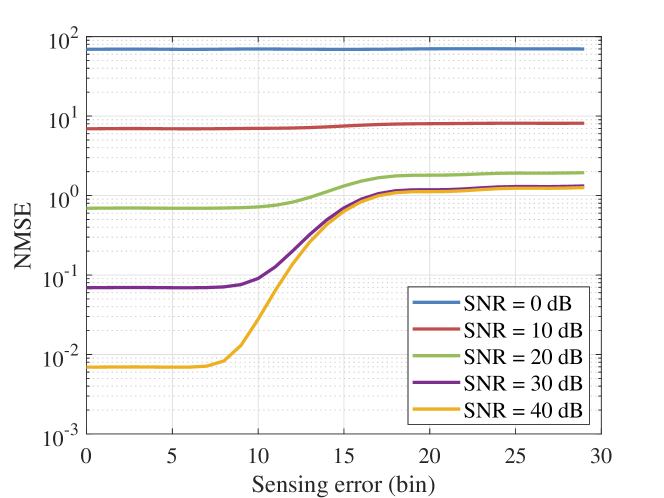
(a) NMSE performance with TF being 10.

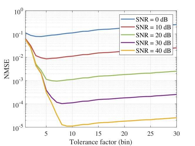
(b) NMSE performance with sensing error being 5 bins.

Figure 4: Impact of tolerance factor on the proposed estimator.

TABLE I: Simulation Parameters for OFDM

Carrier frequency $f_{\mathrm{c}}$	28 GHz	Bandwidth $B$	200 MHz
Subcarrier spacing $\Delta_{\mathrm{f}}$	120 kHz	Symbol duration $T_{\mathrm{o}}$	8.9 $\mu$s
OFDM subcarriers $N$	1584	OFDM symbols $M$	56

The simulation setup of the OFDM system follows 3GPP standards [47], and the parameters adopted in the simulations are listed in Table I. The millimeter wave communications are considered and thus the channel is expected to be sparse. The detailed setup for channels is shown in each case study. The DMRSs are assumed to be uniformly scattered with a subcarrier interval $\Delta_{\text{sc}}=8$ and a symbol interval $\Delta_{\text{sym}}=8$. The 2D FFT uses $N_{\text{Per}}=1024$ and $M_{\text{Per}}=1024$ FFT points for frequency-domain and time-domain processing, respectively. The corresponding FFT bin width under this setup is 1.02 ns and 13.70 Hz for delay and Doppler.

VI-A Numerical Results for Tolerance Factors

First, numerical results for evaluating tolerance factors are presented. The NMSE is calculated based on Eq. (7), where $\hat{\sigma}_{w}^{2}$ is set as $10^{-5}$. Three paths with relative SNRs of $[0,-5,-8]$ dB, $\tau=[100,200,400]$ ns, $f_{\mathrm{d}}=[0,-1.87,3.73]$ kHz are considered. Given this scenario, the impact of sensing error on channel estimation performance with fixed tolerance factors is first examined. Then, we vary the size of tolerance factors and observe the channel estimation performance under fixed estimation errors. NMSE performance under different SNRs is evaluated, as shown in Fig. 4.

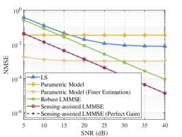
(a) NMSE performance.

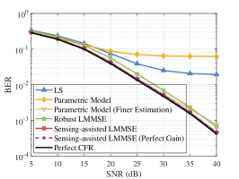
(b) BER performance for 64 QAM.

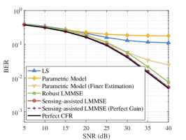
(c) BER performance for 1024 QAM.

Figure 5: Channel estimation performance for a 3-path channel.

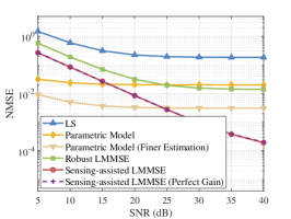
(a) NMSE performance.

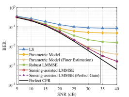
(b) BER performance for 64 QAM.

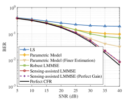
(c) BER performance for 1024 QAM.

Figure 6: Channel estimation performance for a 7-path channel.

The impact of sensing error on the proposed channel estimator is shown in Fig. 4(a). The sensing errors are set to be integer multiples of FFT bin width, and errors are added to the delay and Doppler estimates for every path. The tolerance factors are set to be 10 times the delay bin and Doppler bin i.e., $C_{\mathrm{F},l}=10\tau_{\text{bin}}$ and $C_{\mathrm{T},l}=10f_{\text{d,bin}}$ for every path. The estimator can accommodate sensing deviations up to 5 FFT bins with these tolerance factors. Simulation results show that within 5 bins of delay and Doppler deviation, the NMSE can remain the same. However, when the deviation exceeds the given tolerance factors, the NMSE starts to increase, which happens earlier and more evidently on high SNRs than on low SNRs, indicating that high SNR scenarios are more sensitive to sensing errors. Therefore, the tolerance factors must be designed to effectively account for sensing errors, highlighting the need for the update check in our algorithm.

The impact of the tolerance factor on NMSE is further evaluated in Fig. 4(b). The errors for both delay and Doppler are set to be 5 FFT bins, and the NMSE performance is observed for different tolerance factors. As the tolerance factors increase, the NMSE reduces rapidly when the tolerance factors gradually approach the value required for 5-bin sensing error. After reaching that value, which is 10 bins for the tolerance factor in this case, the NMSE gradually grows as the tolerance factors increase. The smaller the SNR, the less the estimator is influenced by the sensing error. This guides the determination of tolerance factors that they should rather be designed to be large enough to accommodate possible variations in the channel in case the sensing errors in channel parameters are not covered. Therefore, assigning sensing resolution for the tolerance factor would be a preferred choice for multiple reasons including this one.

VI-B Simulation Results for Channel Estimation Performance

Next, the proposed sensing-assisted LMMSE channel estimation method is compared with other channel estimators. Three types of estimators are adopted as the benchmarks: 1) the simplest LS estimator, where LS is applied at pilots with spline interpolation for data symbols; 2) the robust LMMSE estimator, where the maximum delay spread and Doppler spread are assumed to be perfectly achieved and uniform distributions are adopted for the construction of channel correlation matrix; 3) the parametric model-based estimator, where the high-resolution MUSIC algorithm is applied for the estimation of delay and Doppler, and the LMMSE algorithm is further conducted for the estimation of the amplitude of each path, which is an extended method of [27] for the doubly-selective channel. In the parametric model-based method, the accuracy of delay and Doppler estimation depends on the step size in the MUSIC spectrum search. Two cases are considered: 1) the same size as our 2D FFT bin; and 2) a finer estimation with a step size of only 1/4 of the FFT bin for both delay and Doppler estimation. A small step size leads to high accuracy, but highly increases the computational complexity in MUSIC and also the estimation of the amplitude of each path. The sensing algorithm uses $S=10$ to reduce Doppler resolution. The tolerance factors are assigned with the sensing resolution values. The simulation considers two consequent slots. Moreover, to validate the effectiveness of applying a constant multi-path intensity profile in the construction of our channel correlation matrices, i.e., $\theta(\tau_{l})=1$ for $l=1,2,\cdots,\hat{L}$, the results with true multi-path intensity profile (perfect gain) are also provided.

We first evaluate the performance comparison for the 3-path scenario introduced in the previous setup. As shown in Fig. 5(a), the sensing-assisted LMMSE estimator with the assumption of a constant intensity profile performs almost identically to the one with perfect gain as the multi-path intensity profile, suggesting that the path gain estimation is unnecessary in the proposed design. The proposed estimator outperforms nearly all other estimators in terms of NMSE, except for the parametric model-based estimator with finer estimation at low SNRs. The NMSE performance of the parametric model-based estimators highly depends on the sensing accuracy. Thus, its performance gain comes at the expense of increased computational complexity. When SNR grows, sensing error can be critical to the parametric model-based estimator, preventing it from achieving better performance. In addition to NMSE performance, the bit error rate (BER) performance is also evaluated for 64 QAM and 1024 QAM modulations, as shown in Fig. 5(b) and Fig. 5(c), respectively. The BER under perfect CFR is also provided as a lower-bound benchmark. Compared to other schemes, the BER performance of the proposed estimator is consistent with its NMSE performance. Moreover, our scheme can approach the BER performance of perfect CFR in both QAM modulations. The NMSE gain of parametric model-based estimators in low SNR region is not obvious in terms of BER, because all estimators can perform close to the perfect CFR case. The comparison between Fig. 5(b) and Fig. 5(c) also reveals that as the order of modulation grows, the superiority of the proposed estimator becomes more evident, suggesting its applicability in high-data-rate scenarios.

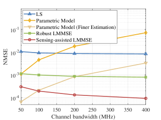
Figure 7: Impact of bandwidth on different channel estimators.

The proposed sensing-assisted LMMSE scheme is then evaluated in a doubly-selective channel with more paths. The paths are characterized by relative SNRs of [0, -1.2, -2.2, -3, -3.2, -3.4, -4] dB, delays of [0, 251, 90, 311, 176, 312, 181] ns, and Doppler shifts of [0, 1.9, -3.7, 4.7, -5.6, 4.7, -1.9] kHz. In this setup, the 4th and the 6th paths are irresolvable in both delay and Doppler. They are detected as one path using the proposed sensing algorithm. Meanwhile, the finer estimation with MUSIC can detect these two paths separately. The tolerance factors are chosen in the same way as the previous results. As shown in Fig. 6, simulation results show a similar trend as compared with Fig. 5. However, when the channel is more complicated, the performance of the two LMMSE-based estimators slightly degrades. It can be concluded that our proposed scheme can significantly outperform the LS and robust LMMSE estimators, especially in high SNR regions, but fails to outperform the parametric model-based estimators in low SNR regions. For example, at a BER of 0.03 for 1024 QAM modulation, the sensing-assisted LMMSE estimator achieves a 7 dB gain compared with the parametric model-based estimator with finer sensing results. Simulation results imply that the proposed algorithm potentially requires fewer pilots to achieve the same BER performance as other channel estimation methods, which will further be evaluated in the following simulations.

Then, the impact of channel bandwidth on the aforementioned channel estimators is compared in Fig. 7 under the 3-path scenario at 30 dB SNR. As shown from the simulation results, the NMSE performance of the parametric model-based estimators decreases as the channel bandwidth increases, while the performance of other estimators improves. This can be explained by the fact that the parametric model-based estimator directly utilizes the sensing results, so the sensing error can be cumulated as the number of subcarriers increases. Thus, it is more sensitive to sensing errors as bandwidth increases. On the other hand, the proposed sensing-assisted LMMSE estimator gives tolerance to the rough estimation result, which leads to its superiority in large bandwidth. This suggests that the proposed estimator is more suitable for large bandwidth channels.

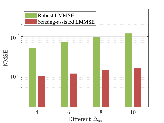
(a) NMSE performance for different pilot subcarrier intervals.

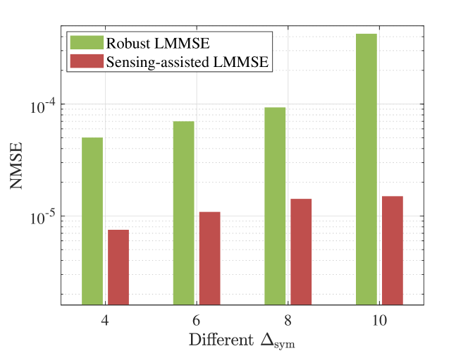
(b) NMSE performance for different pilot symbol intervals.

Figure 8: Impact of the DMRS deployment density on NMSE performance.

Finally, the impact of the pilot interval on the proposed channel estimator is studied. Following the 3-path model used in the previous simulations, the NMSE performance under different DMRS deployments is shown in Fig. 8. A high SNR of 40 dB is considered in this case study, which can support a low BER for high-order modulations. The robust LMMSE estimator is comparable to the proposed estimator, since the robust LMMSE estimator performs better than other benchmarks in high SNR regions. In Fig. 8(a), the symbol interval is set to 8, i.e., $\Delta_{\text{sym}}=8$, and the impact of different subcarrier intervals is evaluated. The proposed estimator outperforms the robust LMMSE estimator for all subcarrier intervals. The performance of our proposed scheme with the subcarrier interval of $\Delta_{\text{sc}}=10$ is still much better than the robust LMMSE scheme with $\Delta_{\text{sc}}=4$. In Fig. 8(b), the pilot subcarrier interval is set fixed, i.e., $\Delta_{\text{sc}}=8$, and the impact of different pilot symbol intervals is evaluated. We can see that our proposed estimator still performs better than the robust LMMSE estimator for all the pilot symbol intervals. Both cases show that with our proposed scheme, the overhead of pilots can be highly reduced, due to the high efficiency of our proposed scheme.

VII Discussions

In this paper, the SISO channel model is considered. However, the design can also be extended to MIMO systems with different beamforming architectures. Let’s consider a general MIMO system as follows. If the BS is equipped with $N_{\mathrm{t}}$ antennas and the user is equipped with $N_{\mathrm{r}}$ antennas, the CFR at the $n$-th subcarrier and $m$-th symbol can be modeled as

$$\mathbf{H}_{n,m}=\sum_{l=1}^{L}\alpha_{l}e^{-j2\pi n\Delta_{\mathrm{f}}\tau_{l}}e^{j2\pi mT_{\mathrm{o}}f_{\mathrm{d},l}}\mathbf{a}_{\mathrm{r}}(\theta_{l})\mathbf{a}_{\mathrm{t}}(\varphi_{l})^{\mathsf{H}},$$ (10)

where $\mathbf{a}_{\mathrm{r}}(\theta_{l})$ and $\mathbf{a}_{\mathrm{t}}(\varphi_{l})$ are the receive and transmit steering vectors, respectively, and $\theta_{l}$ and $\varphi_{l}$ denote the angle of arrival (AoA) and the angle of departure (AoD) for the $l$-th path, respectively.

Compared to the SISO channel model in Eq. (1), the MIMO channel model in Eq. (10) introduces two additional angular parameters for each path, i.e., $\theta_{l}$ and $\varphi_{l}$. These angular parameters can be estimated using sensing algorithms to enhance MIMO channel estimation. However, compared to the estimation of delay and Doppler, angle estimation has some distinct features. The angle estimation relies on the phase difference across antenna ports. Since the signals arrived at all ports are identical, it is unnecessary to know the exact symbol, enabling the use of both pilot symbols and data symbols for angle estimation. The AoA and AoD can be separately estimated or jointly estimated [48, 49]. The angular parameters usually change slowly, allowing sensing algorithms such as MUSIC to be adopted for high-resolution and high-accuracy angular information that assists channel estimation [18]. With the angular estimation, our proposed scheme can be directly applied. How to design an estimator that can jointly utilize angle, delay, and Doppler information from sensing function with low complexity is always an interesting topic, which is subject to our future work.

VIII Conclusion

In bistatic OFDM ISAC systems, sensing information can naturally be utilized to aid communication channel estimation. In this paper, a sensing-assisted framework for bistatic OFDM systems that can leverage the raw sensing results was developed to assist channel estimation. To meet the requirements for real-time decoding, a tailored low-complexity sensing algorithm was adopted. The potential sensing errors caused by the low-complexity sensing algorithms can be tolerated in the proposed sensing-assisted LMMSE algorithm. This approach incorporated specifically designed time-domain and frequency-domain tolerance factors, enabling robust handling of sensing errors. The NMSE performance and computational complexity were analyzed, which provided suggestions for a proper parameter selection in our design. Simulation results demonstrated that the proposed sensing-assisted LMMSE channel estimation method significantly outperforms the other estimation schemes, especially in the case of high SNR regions or large bandwidths, while maintaining low computational complexity, highlighting its potential for practical implementation in future wireless networks.

Appendix A Proof of Theorem 1

Perform SVD on the constructed correlation matrix as

$$\hat{\mathbf{R}}_{\mathbf{h}_{\mathrm{p}}\mathbf{h}_{\mathrm{p}}}=\mathbf{V}\mathbf{\Gamma}\mathbf{V}^{\mathsf{H}},$$

where $\mathbf{V}$ is a unitary matrix, and $\mathbf{\Gamma}$ is a diagonal matrix containing singular values $\gamma_{1}\geq\gamma_{2}\geq\cdots\geq\gamma_{N_{\mathrm{p}}M_{\mathrm{p}}}$. The LMMSE coefficient matrix can thus be expressed as

$$\mathbf{W} =\mathbf{V}\mathbf{\Gamma}\mathbf{V}^{\mathsf{H}}(\mathbf{V}\mathbf{\Gamma}\mathbf{V}^{\mathsf{H}}+\hat{\sigma}_{w}^{2}\mathbf{V}\mathbf{V}^{\mathsf{H}})^{-1}$$

$$=\mathbf{V}\mathbf{\Gamma}(\mathbf{\Gamma}+\hat{\sigma}_{w}^{2}\mathbf{I}_{N_{\mathrm{p}}M_{\mathrm{p}}})^{-1}\mathbf{V}^{\mathsf{H}}$$

$$=\mathbf{V}\mathbf{\Lambda}\mathbf{V}^{\mathsf{H}},$$

where $\mathbf{\Lambda}=\mathbf{\Gamma}(\mathbf{\Gamma}+\hat{\sigma}_{w}^{2}\mathbf{I}_{N_{\mathrm{p}}M_{\mathrm{p}}})^{-1}$ is a diagonal matrix with singular values $\lambda_{1}\geq\lambda_{2}\geq\cdots\geq\lambda_{N_{\mathrm{p}}M_{\mathrm{p}}}$ and $\lambda_{i}=\gamma_{i}/(\gamma_{i}+\hat{\sigma}_{w}^{2})$.

The MSE matrix can thus be expressed as

$$\mathbf{M}_{\mathrm{p}}\!\!=\!\!\mathbf{V}(\mathbf{I}_{N_{\mathrm{p}}M_{\mathrm{p}}}\!\!-\!\mathbf{\Lambda})\mathbf{V}^{\mathsf{H}}\mathbf{R}_{\mathbf{h}_{\mathrm{p}}\mathbf{h}_{\mathrm{p}}}\!\!\mathbf{V}(\mathbf{I}_{N_{\mathrm{p}}M_{\mathrm{p}}}\!\!-\!\mathbf{\Lambda})\mathbf{V}^{\mathsf{H}}\!+\!\sigma_{w}^{2}\mathbf{V}\!\mathbf{\Lambda}\mathbf{\Lambda}^{\mathsf{H}}\mathbf{V}^{\mathsf{H}}\!.$$

The trace operation owns the following properties:

1. $\text{Trace}(\mathbf{V}\mathbf{A}\mathbf{V}^{\mathsf{H}})=\text{Trace}(\mathbf{A})$ if $\mathbf{V}$ is a unitary matrix;

2. $\text{Trace}(\mathbf{V}\mathbf{A}\mathbf{V})=\sum_{i}(\mathbf{V})_{i,i}^{2}(\mathbf{A})_{i,i}$ if $\mathbf{V}$ is a diagonal matrix.

Since $\mathbf{V}$ is unitary, and $\mathbf{I}_{N_{\mathrm{p}}M_{\mathrm{p}}}-\mathbf{\Lambda}$ is diagonal, the resulting NMSE is given by

$$\text{NMSE}_{\mathrm{p}} =\frac{1}{N_{\mathrm{p}}M_{\mathrm{p}}}\text{Trace}(\mathbf{M}_{\mathrm{p}})$$

$$=\frac{1}{N_{\mathrm{p}}M_{\mathrm{p}}}\left[\Sigma_{i=1}^{N_{\mathrm{p}}M_{\mathrm{p}}}\left((1-\lambda_{i})^{2}b_{i}+\sigma_{w}^{2}\lambda_{i}^{2}\right)\right],$$

where $\mathbf{B}=\mathbf{V}^{\mathsf{H}}\mathbf{R}_{\mathbf{h}_{\mathrm{p}}\mathbf{h}_{\mathrm{p}}}\mathbf{V}$, and the diagonal elements of $\mathbf{B}$ is denoted as $(\mathbf{B})_{i,i}=b_{i}$.

References

- [1] S. Wang, A. Tang, X. Wang, and W. Qu, “Sensing-Assisted Channel Estimation for OFDM ISAC Systems,” in Proc. IEEE ICC, 2025.
- [2] 3GPP, “Feasibility Study on Integrated Sensing and Communication,” Tech. Rep. TR 22.837 version 19.2.1, Feb. 2024.
- [3] A. R. Chiriyath, B. Paul, and D. W. Bliss, “Radar-Communications Convergence: Coexistence, Cooperation, and Co-Design,” IEEE Trans. Cognitive Commun. Net., vol. 3, no. 1, pp. 1–12, 2017.
- [4] F. Liu, Y. Cui, C. Masouros, J. Xu, T. X. Han, Y. C. Eldar, and S. Buzzi, “Integrated Sensing and Communications: Toward Dual-Functional Wireless Networks for 6G and Beyond,” IEEE J. Sel. Areas Commun., vol. 40, no. 6, pp. 1728–1767, 2022.
- [5] J. A. Zhang, M. L. Rahman, K. Wu, X. Huang, Y. J. Guo, S. Chen, and J. Yuan, “Enabling Joint Communication and Radar Sensing in Mobile Networks—A Survey,” IEEE Commun. Surveys Tutorials, vol. 24, no. 1, pp. 306–345, 2022.
- [6] Z. Wei, Y. Wang, L. Ma, S. Yang, Z. Feng, C. Pan, Q. Zhang, Y. Wang, H. Wu, and P. Zhang, “5G PRS-based sensing: A sensing reference signal approach for joint sensing and communication system,” IEEE Trans. Veh. Technol., vol. 72, no. 3, pp. 3250–3263, 2022.
- [7] Q. Zhao, A. Tang, and X. Wang, “Reference Signal Design and Power Optimization for Energy-Efficient 5G V2X Integrated Sensing and Communications,” IEEE Trans. Green Commun. Net., vol. 7, no. 1, pp. 379–392, 2023.
- [8] Z. He, W. Xu, H. Shen, D. W. K. Ng, Y. C. Eldar, and X. You, “Full-duplex communication for ISAC: Joint beamforming and power optimization,” IEEE J. Sel. Areas Commun., vol. 41, no. 9, pp. 2920–2936, 2023.
- [9] H. Hua, J. Xu, and T. X. Han, “Optimal transmit beamforming for integrated sensing and communication,” IEEE Trans. Veh. Technol., vol. 72, no. 8, pp. 10 588–10 603, 2023.
- [10] S. Lu, F. Liu, F. Dong, Y. Xiong, J. Xu, Y.-F. Liu, and S. Jin, “Random ISAC signals deserve dedicated precoding,” IEEE Trans. Signal Process., 2024.
- [11] Z. Wei, R. Yao, X. Yuan, H. Wu, Q. Zhang, and Z. Feng, “Precoding optimization for MIMO-OFDM integrated sensing and communication systems,” IEEE Trans. Cognitive Commun. Net., 2024.
- [12] Z. Ren, L. Qiu, J. Xu, and D. W. K. Ng, “Sensing-Assisted Sparse Channel Recovery for Massive Antenna Systems,” IEEE Trans. Veh. Technol., vol. 73, no. 11, pp. 17 824–17 829, 2024.
- [13] C. Qing, W. Hu, Z. Liu, G. Ling, X. Cai, and P. Du, “Sensing-Aided Channel Estimation in OFDM Systems by Leveraging Communication Echoes,” IEEE Internet of Things J., vol. 11, no. 23, pp. 38 023–38 039, 2024.
- [14] Z. Huang, K. Wang, A. Liu, Y. Cai, R. Du, and T. X. Han, “Joint Pilot Optimization, Target Detection and Channel Estimation for Integrated Sensing and Communication Systems,” IEEE Trans. Wireless Commun., vol. 21, no. 12, pp. 10 351–10 365, 2022.
- [15] Z. Chen, M.-M. Zhao, M. Li, F. Xu, Q. Wu, and M.-J. Zhao, “Joint Location Sensing and Channel Estimation for IRS-Aided mmWave ISAC Systems,” IEEE Trans. Wireless Commun., vol. 23, no. 9, pp. 11 985–12 002, 2024.
- [16] R. Zhang, L. Cheng, S. Wang, Y. Lou, Y. Gao, W. Wu, and D. W. K. Ng, “Integrated Sensing and Communication With Massive MIMO: A Unified Tensor Approach for Channel and Target Parameter Estimation,” IEEE Trans. Wireless Commun., vol. 23, no. 8, pp. 8571–8587, 2024.
- [17] X. Chen, Z. Feng, J. Andrew Zhang, Z. Wei, X. Yuan, and P. Zhang, “Sensing-Aided Uplink Channel Estimation for Joint Communication and Sensing,” IEEE Wireless Commun. Lett., vol. 12, no. 3, pp. 441–445, 2023.
- [18] J. Xu, H. Wang, Y. Zeng, and X. Xu, “Little Pilot is Needed for Channel Estimation with Integrated Super-Resolution Sensing and Communication,” in Proc. IEEE WCNC, 2024, pp. 1–6.
- [19] Y. Zhang, L. Huang, and J. Song, “Phased Array Radar Based Angular Domain Channel Estimation Scheme for Integrated Radar-Communication System,” in Proc. IEEE MILCOM, 2016, pp. 906–911.
- [20] K. Xu, X. Xia, C. Li, C. Wei, W. Xie, and Y. Shi, “Channel Feature Projection Clustering Based Joint Channel and DoA Estimation for ISAC Massive MIMO OFDM System,” IEEE Trans. Veh. Technol., vol. 73, no. 3, pp. 3678–3689, 2024.
- [21] X. Chen, Z. Feng, J. A. Zhang, F. Gao, X. Yuan, Z. Yang, and P. Zhang, “Complex CNN CSI Enhancer for Integrated Sensing and Communications,” IEEE J. Sel. Topics Signal Processing, vol. 18, no. 5, pp. 752–765, 2024.
- [22] C. Luo, A. Tang, F. Gao, J. Liu, and X. Wang, “Channel Modeling Framework for Both Communications and Bistatic Sensing Under 3GPP Standard,” IEEE J. Sel. Areas Sensors, vol. 1, pp. 166–176, 2024.
- [23] P. Zhu, H. Lin, J. Li, D. Wang, and X. You, “High-Performance Channel Estimation for mmWave Wideband Systems With Hybrid Structures,” IEEE Trans. Commun., vol. 71, no. 4, pp. 2503–2516, 2023.
- [24] R. Shafin, M. Jiang, S. Ma, L. Piazzi, and L. Liu, “Joint Parametric Channel Estimation and Performance Characterization for 3D Massive MIMO OFDM Systems,” in Proc. IEEE ICC, 2018, pp. 1–6.
- [25] S. Liu, F. Wang, R. Zhang, and Y. Liu, “A Simplified Parametric Channel Estimation Scheme for OFDM Systems,” IEEE Trans. Wireless Commun., vol. 7, no. 12, pp. 5082–5090, 2008.
- [26] Z. Gao, L. Dai, Z. Lu, C. Yuen, and Z. Wang, “Super-Resolution Sparse MIMO-OFDM Channel Estimation Based on Spatial and Temporal Correlations,” IEEE Commun. Letters, vol. 18, no. 7, pp. 1266–1269, 2014.
- [27] B. Yang, K. Letaief, R. Cheng, and Z. Cao, “Channel Estimation for OFDM Transmission in Multipath Fading Channels Based on Parametric Channel Modeling,” IEEE Trans. Commun., vol. 49, no. 3, pp. 467–479, 2001.
- [28] L. Ge, Y. Zhang, G. Chen, and J. Tong, “Compression-Based LMMSE Channel Estimation With Adaptive Sparsity for Massive MIMO in 5G Systems,” IEEE Syst. J., vol. 13, no. 4, pp. 3847–3857, 2019.
- [29] S. Huang, M. Zhang, Y. Gao, and Z. Feng, “MIMO Radar Aided mmWave Time-Varying Channel Estimation in MU-MIMO V2X Communications,” IEEE Trans. Wireless Commun., vol. 20, no. 11, pp. 7581–7594, 2021.
- [30] H.-R. Park, “Adaptive Channel Estimation for OFDM Systems Using CIR Length Estimate,” IEEE Wireless Commun. Lett., vol. 10, no. 11, pp. 2597–2601, 2021.
- [31] K.-C. Hung and D. W. Lin, “Pilot-Based LMMSE Channel Estimation for OFDM Systems With Power–Delay Profile Approximation,” IEEE Trans. Veh. Technol., vol. 59, no. 1, pp. 150–159, 2010.
- [32] J. Fang, X. Li, H. Li, and F. Gao, “Low-Rank Covariance-Assisted Downlink Training and Channel Estimation for FDD Massive MIMO Systems,” IEEE Trans. Wireless Commun., vol. 16, no. 3, pp. 1935–1947, 2017.
- [33] H. Xie, F. Gao, S. Jin, J. Fang, and Y.-C. Liang, “Channel Estimation for TDD/FDD Massive MIMO Systems With Channel Covariance Computing,” IEEE Trans. Wireless Commun., vol. 17, no. 6, pp. 4206–4218, 2018.
- [34] O. Edfors, M. Sandell, J.-J. van de Beek, S. Wilson, and P. Borjesson, “OFDM Channel Estimation by Singular Value Decomposition,” IEEE Trans. Commun., vol. 46, no. 7, pp. 931–939, 1998.
- [35] Y. Li, L. Cimini, and N. Sollenberger, “Robust Channel Estimation for OFDM Systems with Rapid Dispersive Fading Channels,” IEEE Trans. Commun., vol. 46, no. 7, pp. 902–915, 1998.
- [36] P. Hoeher, S. Kaiser, and P. Robertson, “Two-dimensional pilot-symbol-aided channel estimation by Wiener filtering,” in Proc. IEEE Int. Conf. on Acoust., Speech, and Signal Process., vol. 3, 1997, pp. 1845–1848 vol.3.
- [37] S. Li, C. Luo, A. Tang, X. Wang, C. Xu, F. Gao, and L. Cai, “Integrating Passive Bistatic Sensing into mmWave B5G/6G Networks: Design and Experiment Measurement,” in Proc. IEEE ICC, 2023, pp. 2952–2957.
- [38] C. Sturm and W. Wiesbeck, “Waveform Design and Signal Processing Aspects for Fusion of Wireless Communications and Radar Sensing,” Proc. IEEE, vol. 99, no. 7, pp. 1236–1259, 2011.
- [39] K. M. Braun, OFDM Radar Algorithms in Mobile Communication Networks. Ph.D. dissertation, Karlsruher Institut für Technologie (KIT), Karlsruhe, Germany, 2014.
- [40] J.-J. van de Beek, O. Edfors, M. Sandell, S. Wilson, and P. Borjesson, “On Channel Estimation in OFDM Systems,” in Proc. IEEE VTC, vol. 2, 1995, pp. 815–819 vol.2.
- [41] M. Šimko, C. Mehlführer, M. Wrulich, and M. Rupp, “Doubly Dispersive Channel Estimation with Scalable Complexity,” in IEEE WSA, 2010, pp. 251–256.
- [42] D. Rife and R. Boorstyn, “Single Tone Parameter Estimation from Discrete-Time Observations,” IEEE Trans. Inf. Theory, vol. 20, no. 5, pp. 591–598, 1974.
- [43] H. So, Y. Chan, Q. Ma, and P. Ching, “Comparison of Various Periodograms for Sinusoid Detection and Frequency Estimation,” IEEE Trans. Aerosp. Electron. Syst., vol. 35, no. 3, pp. 945–952, 1999.
- [44] F. Harris, “On The Use of Windows for Harmonic Analysis with The Discrete Fourier Transform,” Proc. IEEE, vol. 66, no. 1, pp. 51–83, 1978.
- [45] A. Assalini, E. Dall’Anese, and S. Pupolin, “Linear MMSE MIMO Channel Estimation with Imperfect Channel Covariance Information,” in Proc. IEEE ICC, 2009, pp. 1–5.
- [46] Y. Choi, J. H. Bae, and J. Lee, “Low-Complexity 2D LMMSE Channel Estimation for OFDM Systems,” in Proc. IEEE VTC-Fall, 2015, pp. 1–5.
- [47] 3GPP, “NR; Physical Channels and Modulation,” Tech. Rep. TS 38.211 version 18.4.0, Sep. 2024.
- [48] W. Zhang, M. Dong, and T. Kim, “MMV-Based Sequential AoA and AoD Estimation for Millimeter Wave MIMO Channels,” IEEE Trans. Commun., vol. 70, no. 6, pp. 4063–4077, 2022.
- [49] C.-Y. Chen and W.-R. Wu, “Joint AoD, AoA, and Channel Estimation for MIMO-OFDM Systems,” IEEE Trans. Veh. Technol., vol. 67, no. 7, pp. 5806–5820, 2018.