Inverse scattering transform for the defocusing local-and-nonlocal nonlinear Schrödinger equation with non-zero boundary conditions

Abstract

By the Riemann-Hilbert method, the theory of inverse scattering transform is developed for the defocusing local-and-nonlocal nonlinear Schrödinger equation (which originates from the parity-symmetric reduction of the Manakov system) with non-zero boundary conditions. First, the adjoint Lax pair and auxiliary eigenfunctions are introduced for the direct scattering, and the analyticity, symmetries of eigenfunctions and scattering matrix are studied in detail. Then, the distribution of discrete eigenvalues is examined, and the asymptotic behaviors of the eigenfunctions and scattering coefficients are analyzed rigorously. Compared with the Manakov system, the reverse-space nonlocality introduces an additional symmetry, leading to stricter constraints on eigenfunctions, scattering coefficients and norming constants. Further, the Riemann-Hilbert problem is formulated for the inverse problem, and the reconstruction formulas are derived by considering arbitrary simple zeros of scattering coefficients. In the reflectionless case, the N-soliton solutions are presented in the determinant form. With N=1, the dark and beating one-soliton solutions are obtained, which are respectively associated with a pair of discrete eigenvalues lying on and off the circle on the spectrum plane. Via the asymptotic analysis, the two-soliton solutions are found to admit the interactions between two dark solitons or two beating solitons, as well as the superpositions of two beating solitons or one beating soliton and one dark soliton.

Keywords: Inverse scattering transform; Local-and-nonlocal nonlinear Schrödinger equation; N-soliton solutions; Riemann-Hilbert method

1 Introduction

Over the past ten years, the nonlocal nonlinear evolution equations (NEEs) have attracted much attention in the area of integrable systems. In 2013, Ablowitz and Musslimani first proposed the following reverse-space nonlocal nonlinear Schrödinger (NLS) equation [2]:

$$\mathrm{i}q_{t}(x,t)=q_{xx}(x,t)+2\sigma q^{2}(x,t)q^{*}(-x,t),$$ (1.1)

where $q(x,t)$ is a complex-valued function of real variables $x$ and $t$, the asterisk denotes complex conjugate, $\sigma=1$ and $\sigma=-1$ represent the focusing $(+)$ and defocusing $(-)$ nonlinearities, respectively. In contrast to the celebrated NLS equation, the nonlocality of Eq. (1.1) lies in that the nonlinear term depends on the values of the solutions both at the positions $x$ and $-x$. Also, this equation is said to be parity-time (PT) symmetric since the self-induced potential $2\sigma q(x,t)q^{*}(-x,t)$ in Eq. (1.1) is generally complex and PT-symmetric [2, 3, 4, 5]. Remarkably, Eq. (1.1) can arise from the Ablowitz-Kaup-Newell-Segur spectral problem with the PT symmetric reduction (space reversal and complex conjugation), and thus it admits the Lax pair and an infinite number of conservation laws. Recently, much attention was paid to its mathematical properties [2, 4, 6, 7, 8, 9, 10, 11, 12, 13, 14] and various localized-wave solutions [2, 4, 15, 3, 5, 16, 18, 21, 19, 17, 20, 22, 23, 24, 25, 26, 27]. At the same time, the reverse-space, reverse-time and reverse-space-time nonlocal reductions were examined in the traditional soliton equation hierarchies. As a consequence, researchers discovered a number of nonlocal integrable NEEs, spanning from 1+1 and 1+2 dimensions to semi-discrete settings [29, 3, 40, 32, 33, 34, 35, 36, 37, 38, 41, 42, 31, 39, 43, 30, 28].

It has been an important concern to establish the physical relevance of nonlocal integrable NEEs [31, 45, 46, 44]. In 2018, with a clear physical motivation, Yang proposed the following integrable nonlocal NLS equation [43]:

$$\mathrm{i}q_{t}(x,t)+q_{xx}(x,t)+2\sigma q(x,t)\big{(}|q(x,t)|^{2}+|q(-x,t)|^{2}\big{)}=0\quad(\sigma=\pm 1),$$ (1.2)

where the self-induced potential $2\sigma\big{(}|q(x,t)|^{2}+|q(-x,t)|^{2}\big{)}$ is real and even-symmetric in $x$. Since the nonlinearity contains both the local and nonlocal terms, we refer it to as the local-and-nonlocal NLS equation in this paper. In fact, Eq. (1.2) can be reduced from the Manakov system [47]

$$\mathrm{i}q_{t}(x,t)+q_{xx}(x,t)+2\sigma q(x,t)\big{(}|q(x,t)|^{2}+|r(x,t)|^{2}\big{)}=0,$$ (1.3a)

$$\mathrm{i}r_{t}(x,t)+r_{xx}(x,t)+2\sigma r(x,t)\big{(}|q(x,t)|^{2}+|r(x,t)|^{2}\big{)}=0,$$ (1.3b)

with the symmetric constraint

$$r(x,t)=q(-x,t).$$ (1.4)

As we know, the Manakov system is an integrable coupled model which has significant applications in various physical systems with two components/fields interact nonlinearly [48, 49, 47, 50, 51, 54, 52, 53], e.g., the propagation of two orthogonally polarized optical pulses in birefringent fibers [48, 49], the interaction of two incoherent light beams in crystals [50, 51], and the evolution of two atomic clouds with different species in Bose-Einstein condensates [52, 53]. Particularly, when the initial conditions satisfy a parity symmetry constraint between two components/fields, the resultant nonlinear wave dynamics can be governed by the local-and-nonlocal NLS equation (1.2). Therefore, the physical meanings of Eq. (1.2) become evident through its connection with the Manakov system (1.3).

As a physically important nonlocal model, the integrable properties and explicit solutions of Eq. (1.2) were explored in recent years. Based on the soliton solutions of the Manakov system in the Riemann-Hilbert formulation, Yang studied the symmetry relations of discrete scattering data and obtained the bright one- and two-soliton solutions [43]. However, it is hard to derive the N-soliton solutions because the symmetry relations of eigenvectors depend on the number and locations of eigenvalues in a very intricate way. Subsequently, Wu developed the theory of inverse scattering transform (IST) for the initial-value problem of focusing Eq. (1.2) with zero boundary condition (ZBC) [55]. In the framework of Riemann-Hilbert problem (RHP), Ref. [55] performed the spectral analysis from the $t$-part of the Lax pair instead of the $x$-part, and derived the N-soliton solutions in the reflectionless cases. Different from the soliton behaviors in Eq. (1.1), the bright-soliton solutions of Eq. (1.2) are non-singular and can exhibit some interesting dynamics such as the amplitude-changing interactions [43, 55]. In addition, Ref. [56] derived the bright multi-soliton solutions in the determinant form by the Hirota’s bilinear method, and Ref. [57] obtained the multiparametric $N$th-order rogue wave solution in terms of Schur polynomials via the Darboux transformation.

Up to now, there has been no research on the defocusing case of Eq. (1.2), which is expected to admit the dark soliton solutions. In this paper, we develop the IST theory for the defocusing case of Eq. (1.2) with non-zero boundary condition (NZBC), which is given as follows:

$$\displaystyle\lim_{x\to\pm\infty}q(x,t)=q_{\pm}e^{-2\mathrm{i}(|q_{+}|^{2}+|q_{-}|^{2})t},$$ (1.5)

where $q_{\pm}\neq 0$ are independent of $x$ and $t$. By referring to the method for dealing with the defocusing Manakov system in Refs. [60, 58, 59], we introduce an adjoint Lax pair and auxiliary eigenfunctions, provide a rigorous proof for the analyticity and symmetries of the Jost eigenfunctions, auxiliary Jost eigenfunctions and scattering coefficients. In contrast to the Manakov system, the parity-symmetric constraint (1.4) introduces an additional symmetry (see the second symmetry in Section 2.4), which results in stricter constraints on the scattering coefficients, eigenfunctions and norming constants. Moreover, we formulate a matrix RHP for the inverse problem and derive the reconstruction formulas with the presence of arbitrary simple zeros of scattering coefficients. On the other hand, we present the N-soliton solutions in the determinant form for the reflectionless case, and discuss the soliton dynamical behavior based on the distribution of discrete eigenvalues and the asymptotic behavior of solutions. It turns out that the defocusing Eq. (1.2) supports two types of fundamental solitons: the dark soliton and beating soliton, which are respectively linked to the discrete eigenvalue pairs lying on and off the circle on the spectrum plane. We stress that it is a nontrivial task to derive the N-soliton solutions despite they are a subset of Manakov solitons. One may notice that Eq. (1.1) is invariant under the transformation $q(x,t)\to q(-x,t)$, but this invariance does not imply that the admissible solutions of Eq. (1.1) must be even- or odd-symmetric with respect to $x$. For example, the beating one-soliton solution (5.7) does not keep such symmetry in $x$. It should be noted that in the zero-background case of focusing Eq. (1.2), only the multi-soliton solutions with $N>2$ would exhibit asymmetry [43, 55].

The outline of this work is as follows: In Section 2, for the direct scattering we study the analyticity and symmetries of the Jost eigenfunctions, auxiliary Jost eigenfunctions and scattering coefficients. In Section 3, we analyze the distributions and constraints of discrete eigenvalues, and derive the asymptotic behavior of eigenfunctions and analytic scattering coefficients as well as the trace formulas. In Section 4, we construct the RHP, residue conditions and reconstruction formulas. In Section 5, we present the explicit determinant representation of N-soliton solutions, and discuss the soliton dynamical properties based on the distribution of discrete eigenvalues and the asymptotic behavior of solutions. Finally, the conclusions and discussions are presented in Section 6.

2 Direct scattering with NZBC

In this section, we study the direct scattering problem of Eq. (1.2) with NZBC, including the Jost eigenfunctions, auxiliary Jost eigenfunctions and the associated scattering coefficients, as well as their analyticity and symmetries.

2.1 Lax pair, Riemann surface and uniformization

In the defocusing case ($\sigma=-1$) of Eq. (1.2), the Lax pair can be expressed as:

$$\bm{\psi}_{x}(x,t,k)=\mathbf{X}(x,t,k)\bm{\psi}(x,t,k),\quad\mathbf{X}(x,t,k)=-\mathrm{i}k\bm{\sigma}_{3}+\mathbf{Q}(x,t),$$ (2.1a)

$$\bm{\psi}_{t}(x,t,k)=\mathbf{T}(x,t,k)\bm{\psi}(x,t,k),\quad\mathbf{T}(x,t,k)=2k\mathbf{X}(x,t,z)+\mathrm{i}\bm{\sigma}_{3}\mathbf{Q}_{x}(x,t)-\mathrm{i}\bm{\sigma}_{3}{\mathbf{Q}}^{2}(x,t),$$ (2.1b)

with

$$\bm{\sigma}_{3}=\left(\begin{array}[]{ccc}1&0&0\\ 0&1&0\\ 0&0&-1\\ \end{array}\right), \mathbf{Q}(x,t)=\left(\begin{array}[]{ccc}0&0&q(x,t)\\ 0&0&q(-x,t)\\ q^{*}(x,t)&q^{*}(-x,t)&0\\ \end{array}\right),$$ (2.2)

where $\bm{\psi}(x,t,k)$ is the $3\times 3$ matrix, $k\in\mathbb{C}$ is the spectral parameter, and the asterisk represents complex conjugate. Eq. (1.2) is equivalent to the zero-curvature condition $\mathbf{X}_{t}(x,t,k)-\mathbf{T}_{x}(x,t,k)+[\mathbf{X}(x,t,k),\mathbf{T}(x,t,k)]=0$ (also known as the compatibility condition).

To make the boundary conditions independent of $t$, we make the transformation $q(x,t)\to\hat{q}(x,t)e^{-2\mathrm{i}(|q_{+}|^{2}+|q_{-}|^{2})t}$ for Eq. (1.2), obtaining that

$$\mathrm{i}q_{t}(x,t)+q_{xx}(x,t)-2q(x,t)\big{(}|q(x,t)|^{2}+|q(-x,t)|^{2}-2q^{2}_{0}\big{)}=0,$$ (2.3)

where $q_{0}^{2}:=(|q_{+}|^{2}+|q_{-}|^{2})/2$, $q_{0}>0$ and the hat has been dropped for simplicity. Thus, the corresponding NZBC becomes

$$\displaystyle\lim_{x\to\pm\infty}q(x,t)=q_{\pm}.$$ (2.4)

Obviously, if $q(x,t)$ is a solution to Eq. (2.3), then $q(x,t)e^{-4\mathrm{i}q^{2}_{0}t}$ must exactly satisfy Eq. (1.2). Meanwhile, the Lax pair of Eq. (2.3) becomes

$$\bm{\phi}_{x}(x,t,k)=\mathbf{X}(x,t,k)\bm{\phi}(x,t,k),\quad\mathbf{X}(x,t,k)=-\mathrm{i}k\bm{\sigma}_{3}+\mathbf{Q}(x,t),$$ (2.5a)

$$\bm{\phi}_{t}(x,t,k)=\mathbf{T}(x,t,k)\bm{\phi}(x,t,k),\quad\mathbf{T}(x,t,k)=2k\mathbf{X}(x,t,k)+\mathrm{i}\bm{\sigma}_{3}\mathbf{Q}_{x}(x,t)-\mathrm{i}\bm{\sigma}_{3}{\mathbf{Q}}^{2}(x,t)-\mathbf{V_{0}},$$ (2.5b)

where $\bm{\phi}(x,t,k)=e^{-\mathbf{V}_{0}t}\bm{\psi}(x,t,k)$ with $\mathbf{V}_{0}=\mathrm{diag}(-2\mathrm{i}q^{2}_{0},-2\mathrm{i}q^{2}_{0},2\mathrm{i}q^{2}_{0})$.

Keeping in mind (2.4) and taking the limits of Eqs. (2.5) as $x\to\pm\infty$, we derive the asymptotic scattering problem:

$$\bm{\phi}_{\pm,x}(x,t,k)=\mathbf{X}_{\pm}(k)\bm{\phi}_{\pm}(x,t,k),\,\,\bm{\phi}_{\pm,t}(x,t,k)=\mathbf{T}_{\pm}(k)\bm{\phi}_{\pm}(x,t,k),$$ (2.6)

where

$$\mathbf{X}_{\pm}(k)=\left(\begin{array}[]{ccc}-\mathrm{i}k&0&q_{\pm}\\ 0&-\mathrm{i}k&q_{\mp}\\ q^{*}_{\pm}&q^{*}_{\mp}&\mathrm{i}k\\ \end{array}\right),\,\,$$ (2.7d)

$$\mathbf{T}_{\pm}(k)=\left(\begin{array}[]{ccc}-\mathrm{i}|q_{\pm}|^{2}-2\mathrm{i}k^{2}+2\mathrm{i}q_{0}^{2}&-\mathrm{i}q_{\pm}q^{*}_{\mp}&2kq_{\pm}\\ -\mathrm{i}q_{\mp}q^{*}_{\pm}&-\mathrm{i}|q_{\mp}|^{2}-2\mathrm{i}k^{2}+2\mathrm{i}q_{0}^{2}&2kq_{\mp}\\ 2kq^{*}_{\pm}&2kq^{*}_{\mp}&2\mathrm{i}k^{2}\\ \end{array}\right).$$ (2.7h)

Since the matrices $\mathbf{X}_{\pm}(k)$ and $\mathbf{T}_{\pm}(k)$ are independent of $x$ and $t$, the compatibility condition of Eqs. (2.6) becomes $[\mathbf{X}_{\pm}(k),\mathbf{T}_{\pm}(k)]=0$. So, $\mathbf{X}_{\pm}(k)$ and $\mathbf{T}_{\pm}(k)$ share the common eigenfunctions, and their eigenvalues can be, respectively, given by $\{-\mathrm{i}k$, $\pm\mathrm{i}\lambda\}$ and $\{-2\mathrm{i}k^{2}+2\mathrm{i}q^{2}_{0}$, $\pm 2\mathrm{i}k\lambda\}$, where

$$\lambda(k)=\sqrt{k^{2}-2q^{2}_{0}},$$ (2.8)

which shows that the eigenvalues have the branching. To deal with this difficulty, we introduce the two-sheeted Riemann surface so that $\lambda(k)$ is single-valued on each sheet. The branch points occur at $k=\pm\sqrt{2}q_{0}$, thus we can take the branch cut to be the interval $(-\infty,-\sqrt{2}q_{0}]\cup[\sqrt{2}q_{0},\infty)$. For convenience, the regions with $\mathrm{Im}(\lambda)>0$ and $\mathrm{Im}(\lambda)<0$ are denoted as the first and second sheets, respectively.

In order to avoid the direct treatment of the two-sheeted Riemann surface, the following uniformization variable is introduced

$$z=k+\lambda(k),$$ (2.9)

which allows us to work in the complex $z$-plane. Meanwhile, the inverse transformation is given by

$$k=\frac{1}{2}(z+\frac{2q^{2}_{0}}{z}),\,\,\lambda=\frac{1}{2}(z-\frac{2q^{2}_{0}}{z}).$$ (2.10)

Based on the transformation (2.9), the branch cut on either sheet of the Riemann surface is mapped to the real $z$-axis, and the two sheets of the Riemann surface are mapped onto the regions $C^{+}$ and $C^{-}$, which correspond to $\mathrm{Im}(z)>0$ and $\mathrm{Im}(z)<0$, respectively.

Figure 1: The complex $z$-plane, showing the discrete eigenvalues and the regions $C^{+}$ with $\mathrm{Im}(z)>0$ (gray) and $C^{-}$ with $\mathrm{Im}(z)<0$ (white), where $\Gamma$ represents the circle with radius $\sqrt{2}|q_{0}|$. The orientations of the contours for the RHP as well as the symmetries of the discrete eigenvalues in the scattering problem are also displayed.

2.2 Jost eigenfunctions and scattering matrix

Now, we present the Jost eigenfunctions over the continuous spectrum $\Sigma_{z}:\mathbb{R}$, in which $\lambda(k)$ is a real number. The eigenvector matrice of the asymptotic scattering problems (2.6) can be formulated as

$$\mathbf{Y}_{\pm}(z)=\left(\begin{array}[]{ccc}\frac{q_{\pm}}{q_{0}}&-\frac{q^{*}_{\mp}}{\sqrt{2}q_{0}}&\frac{-\mathrm{i}\sqrt{2}q_{\pm}}{z}\\ \frac{q_{\mp}}{q_{0}}&\frac{q^{*}_{\pm}}{\sqrt{2}q_{0}}&\frac{-\mathrm{i}\sqrt{2}q_{\mp}}{z}\\ \frac{2\mathrm{i}q_{0}}{z}&0&\sqrt{2}\\ \end{array}\right),$$ (2.11)

which can diagonalize $\mathbf{X}_{\pm}$ and $\mathbf{T}_{\pm}$ as

$$\mathbf{Y}^{-1}_{\pm}(z)\mathbf{X}_{\pm}(z)\mathbf{Y}_{\pm}(z)=\mathrm{i}\mathbf{J}(z)=\mathrm{diag}(-\mathrm{i}\lambda,-\mathrm{i}k,\mathrm{i}\lambda),$$ (2.12)

$$\mathbf{Y}^{-1}_{\pm}(z)\mathbf{T}_{\pm}(z)\mathbf{Y}_{\pm}(z)=\mathrm{i}\bm{\Omega}(z)=\mathrm{diag}(-2\mathrm{i}k\lambda,-2\mathrm{i}k^{2}+2\mathrm{i}q^{2}_{0},2\mathrm{i}k\lambda).$$

For all $z\in\mathbb{R}$, we define the Jost eigenfunctions $\bm{\phi}_{\pm}(x,t,z)$ as the simultaneous solutions of both the parts of Lax pair (2.5), which satisfy the asymptotic behavior

$$\bm{\phi}_{\pm}(x,t,z)\sim\mathbf{Y}_{\pm}(z)\mathbf{E}(x,t,z)+o(1),\quad x\to\pm\infty,$$ (2.13)

where $\mathbf{E}(x,t,z)=e^{\mathrm{i}\bm{\Theta}(x,t,z)}$ and $\bm{\Theta}(x,t,z)$ is the $3\times 3$ diagonal matrix

$$\bm{\Theta}(x,t,z)=\mathbf{J}(z)x+\bm{\Omega}(z)t=\mathrm{diag}[\theta_{1}(x,t,z),\theta_{2}(x,t,z),-\theta_{1}(x,t,z)],$$ (2.14)

with $\theta_{1}(x,t,z)=-\lambda x-2k\lambda t,\,\theta_{2}(x,t,z)=-kx-2(k^{2}-q^{2}_{0})t$.

Based on the modified Lax pair (2.5), we can obtain the total differential form

$$d\big{(}\mathbf{E}^{-1}(x,t,z)\mathbf{Y}^{-1}_{\pm}(z)\bm{\phi}_{\pm}(x,t,z)\big{)}= \big{(}\mathbf{E}^{-1}(x,t,z)\mathbf{Y}^{-1}_{\pm}(z)\bm{\Delta}\!\mathbf{Q}_{\pm}(x,t)\bm{\phi}_{\pm}(x,t,z)\big{)}dx$$ (2.15)

$$+\big{(}\mathbf{E}^{-1}(x,t,z)\mathbf{Y}^{-1}_{\pm}(z)\bm{\Delta}\!\mathbf{T}_{\pm}(x,t,z)\bm{\phi}_{\pm}(x,t,z)\big{)}dt,$$

where $\bm{\Delta}\!\mathbf{Q}_{\pm}(x,t):=\mathbf{Q}(x,t)-\mathbf{Q}_{\pm}$ and $\bm{\Delta}\!\mathbf{T}_{\pm}(x,t,z):=\mathbf{T}(x,t,z)-\mathbf{T}_{\pm}(x,t,z)=2k\bm{\Delta}\!\mathbf{Q}_{\pm}(x,t)+\mathrm{i}\mathbf{Q}_{x}(x,t)\bm{\sigma_{3}}+\mathrm{i}\bm{\sigma}_{3}\mathbf{Q}^{2}(x,t)-\mathrm{i}\bm{\sigma_{3}}\mathbf{Q}^{2}_{\pm}$. Thus, choosing the integration paths $(-\infty,t)\to(x,t)$ and $(x,t)\to(\infty,t)$, the Jost eigenfunctions $\bm{\phi}_{\pm}(x,t,z)$ can be uniquely determined by two Volterra integral equations:

$$\bm{\phi}_{-}(x,t,z)=\mathbf{Y}_{-}(z)\mathbf{E}(x,t,z)+\int_{-\infty}^{x}\mathbf{Y}_{-}(z)e^{\mathrm{i}\mathbf{J}(z)(x-y)}\mathbf{Y}^{-1}_{-}(z)\bm{\Delta}\!\mathbf{Q}_{-}(y,t,z)\bm{\phi}_{-}(y,t,z)dy,$$ (2.16a)

$$\bm{\phi}_{+}(x,t,z)=\mathbf{Y}_{+}(z)\mathbf{E}(x,t,z)-\int_{x}^{\infty}\mathbf{Y}_{+}(z)e^{\mathrm{i}\mathbf{J}(z)(x-y)}\mathbf{Y}^{-1}_{+}(z)\bm{\Delta}\!\mathbf{Q}_{+}(y,t,z)\bm{\phi}_{+}(y,t,z)dy.$$ (2.16b)

To factorize the exponential oscillations of $\bm{\phi}_{\pm}(x,t,z)$, we further introduce the modified Jost eigenfunctions

$$\bm{\mu}_{\pm}(x,t,z)=\bm{\phi}_{\pm}(x,t,z)\mathbf{E}^{-1}(x,t,z),$$ (2.17)

such that $\displaystyle\lim_{x\to\pm\infty}\bm{\mu}_{\pm}(x,t,z)=\mathbf{Y}_{\pm}(z)$. Then, we can obtain the analyticity of modified Jost eigenfunctions $\bm{\mu}_{\pm}$ (see Appendix A.1):

Theorem 2.1

Suppose $||\bm{\Delta}\!\mathbf{Q}_{\pm}(\cdot,t)||\in L^{1}(\mathbb{R})$, the following columns of $\bm{\mu}_{+}(x,t,z)$ and $\bm{\mu}_{-}(x,t,z)$ can be analytically extended into the corresponding regions of the complex $z$-plane:

$$\mu_{-,1}(x,t,z),\mu_{+,3}(x,t,z):C^{+};\quad\mu_{+,1}(x,t,z),\mu_{-,3}(x,t,z):C^{-},$$ (2.18)

where the subscripts denote matrix columns, i.e., $\bm{\mu}_{\pm}(x,t,z)=(\mu_{\pm,1}(x,t,z),\mu_{\pm,2}(x,t,z),\mu_{\pm,3}(x,t,z))$.

In view of Eq. (2.17), the corresponding columns of $\bm{\phi}_{\pm}(x,t,z)$ possess the same analyticity and boundedness properties. However, $\bm{\mu}_{\pm,2}(x,t,z)$ (or $\bm{\phi}_{\pm,2}(x,t,z))$ are nowhere analytic in general.

For convenience, we define that $\gamma(z):=\mathrm{det}(\mathbf{Y}_{\pm}(z))=2-4q^{2}_{0}/z^{2}$, and then introduce the scattering matrix. If $\bm{\phi}(x,t,z)$ satisfies (2.5), taking the derivatives of $e^{-\mathrm{i}\bm{\Theta}(x,t,z)}\bm{\phi}(x,t,z)$ with respect to $x$ and $t$ yields

$$\frac{\partial}{\partial x}\big{[}e^{-\mathrm{i}\bm{\Theta}(x,t,z)}\bm{\phi}(x,t,z)\big{]}=\big{[}-\mathrm{i}\mathbf{J}(z)e^{-\mathrm{i}\bm{\Theta}(x,t,z)}+e^{-\mathrm{i}\bm{\Theta}(x,t,z)}\mathbf{X}(x,t,z)\big{]}\bm{\phi}(x,t,z),$$ (2.19)

$$\frac{\partial}{\partial t}\big{[}e^{-\mathrm{i}\bm{\Theta}(x,t,z)}\bm{\phi}(x,t,z)\big{]}=\big{[}-\mathrm{i}\bm{\Omega}(z)e^{-\mathrm{i}\bm{\Theta}(x,t,z)}+e^{-\mathrm{i}\bm{\Theta}(x,t,z)}\mathbf{T}(x,t,z)\big{]}\bm{\phi}(x,t,z).$$

Noticing that

$$\operatorname{tr}\big{[}-\mathrm{i}\mathbf{J}(z)e^{-\mathrm{i}\bm{\Theta}(x,t,z)}+e^{-\mathrm{i}\bm{\Theta}(x,t,z)}\mathbf{X}(x,t,z)\big{]}=\operatorname{tr}\big{[}-\mathrm{i}\bm{\Omega}(z)e^{-\mathrm{i}\bm{\Theta}(x,t,z)}+e^{-\mathrm{i}\bm{\Theta}(x,t,z)}\mathbf{T}(x,t,z)\big{]}=0,$$ (2.20)

it follows from Abel’s theorem that $\mathrm{det}\big{[}e^{-\mathrm{i}\bm{\Theta}(x,t,z)}\bm{\phi}(x,t,z)\big{]}=\mathrm{det}\big{[}\bm{\phi}(x,t,z)\big{]}e^{-\mathrm{i}\theta_{2}(x,t,z)}$ is independent of $x$ and $t$. Owing to Eq. (LABEL:4), we have

$$\mathrm{det}(\bm{\phi}_{\pm}(x,t,z))=\gamma(z)e^{\mathrm{i}\theta_{2}(x,t,z)}\quad\mathrm{for\,all}\,z\in\Sigma_{o}:\,\mathbb{R}\setminus\{\pm\sqrt{2}q_{0}\}.$$ (2.21)

Recalling that $\bm{\phi}_{+}(x,t,z)$ and $\bm{\phi}_{-}(x,t,z)$ are two fundamental matrix solutions of Eq. (2.6), and there must exist a $3\times 3$ matrix $\mathbf{A}(z)$ such that

$$\bm{\phi}_{-}(x,t,z)=\bm{\phi}_{+}(x,t,z)\mathbf{A}(z),\,\,z\in\Sigma_{o},$$ (2.22)

where $\mathbf{A}(z)=(a_{ij}(z))$ is called the scattering matrix, which has $\mathrm{det}(\mathbf{A}(z))=1$ due to Eq. (2.21). It is also convenient to introduce the matrix $\mathbf{B}(z):=\mathbf{A}^{-1}(z)=(b_{ij}(z))$.

In the three-dimension case, the analyticity of the diagonal scattering coefficients cannot follow trivially from their representations as the Wronskians of eigenfunctions because the non-analyticity of $\bm{\mu}_{\pm,2}(x,t,z)(\bm{\phi}_{\pm,2}(x,t,z))$. Instead, the scattering coefficients $a_{ij}(z)$ and $b_{ij}(z)$ can be represented by

$$a_{ij}(z)=[\bm{\mu}^{-1}_{+}(x,t,z)]^{j}\mu_{-,i}(x,t,z),\quad b_{ij}(z)=[\bm{\mu}^{-1}_{-}(x,t,z)]^{j}\mu_{+,i}(x,t,z),$$ (2.23)

where $[\bm{\mu}^{-1}_{\pm}(x,t,z)]^{j}$ are the $j$th rows of $\bm{\mu}^{-1}_{\pm}(x,t,z)$. As proved in Appendix A.2, we obtain the analyticity of the scattering coefficients

Theorem 2.2

Suppose $||\bm{\Delta}\!\mathbf{Q}_{\pm}(\cdot,t)||\in L^{1}(\mathbb{R})$, the following scattering coefficients can be analytically extended into the corresponding regions of the complex $z$-plane

$$a_{11}(z),\,b_{33}(z):\,C^{+},\quad a_{33}(z),\,b_{11}(z):\,C^{-}.$$ (2.24)

Note that nothing can be proved for the remaining entries of scattering matrix $\mathbf{A}(z)$.

2.3 Adjoint problem and auxiliary eigenfunctions

As we know, it requires a complete set of analytic eigenfunctions to solve the inverse problem. However, $\bm{\phi}_{\pm,2}(x,t,z)$ are in general not analytic in any given region. To overcome this difficulty, in the way of Refs. [60, 58, 59], we consider the adjoint Lax pair:

$$\tilde{\bm{\phi}}_{x}(x,t,k)=\tilde{\mathbf{X}}(x,t,k)\bm{\phi}(x,t,k),\quad\tilde{\bm{\phi}}_{t}(x,t,k)=\tilde{\mathbf{T}}(x,t,k)\bm{\phi}(x,t,k),$$ (2.25a)

with

$$\tilde{\mathbf{X}}(x,t,k)=\mathbf{X}^{*}(x,t,k^{*})=\mathrm{i}k\bm{\sigma}_{3}+\mathbf{Q}^{*}(x,t),$$ (2.26a)

$$\tilde{\mathbf{T}}(x,t,k)=\mathbf{T}^{*}(x,t,k^{*})=2k\tilde{\mathbf{X}}(x,t,k)-\mathrm{i}\bm{\sigma}_{3}\mathbf{Q}^{*}_{x}(x,t)+\mathrm{i}\bm{\sigma}_{3}({\mathbf{Q}^{*}})^{2}(x,t)+\mathbf{V_{0}}.$$ (2.26b)

It is easy to check that Eq. (2.3) can also be obtained from the zero-curvature condition $\tilde{\mathbf{X}}_{x}(x,t,k)-\tilde{\mathbf{T}}_{t}(x,t,k)+[\tilde{\mathbf{X}}(x,t,k),\tilde{\mathbf{T}}(x,t,k)]=0$. Following the same procedure in section 2.2, we obtain the eigenvector matrix of $\tilde{\mathbf{X}}_{\pm}(z)$ and $\tilde{\mathbf{T}}_{\pm}(z)$:

$$\tilde{\mathbf{Y}}_{\pm}(z)=\mathbf{Y}^{*}_{\pm}(z^{*})=\left(\begin{array}[]{ccc}\frac{q^{*}_{\pm}}{q_{0}}&-\frac{q_{\mp}}{\sqrt{2}q_{0}}&\frac{\mathrm{i}\sqrt{2}q^{*}_{\pm}}{z}\\ \frac{q^{*}_{\mp}}{q_{0}}&\frac{q_{\pm}}{\sqrt{2}q_{0}}&\frac{\mathrm{i}\sqrt{2}q^{*}_{\mp}}{z}\\ \frac{-2\mathrm{i}q_{0}}{z}&0&\sqrt{2}\\ \end{array}\right),$$ (2.27)

which has $\mathrm{det}(\tilde{\mathbf{Y}}_{\pm}(z))=\gamma(z)$ and can make $\tilde{\mathbf{Y}}^{-1}_{\pm}(z)\tilde{\mathbf{X}}_{\pm}(z)\tilde{\mathbf{Y}}_{\pm}(z)=-\mathrm{i}\mathbf{J}(z)$ and $\tilde{\mathbf{Y}}^{-1}_{\pm}(z)\tilde{\mathbf{T}}_{\pm}(z)\tilde{\mathbf{Y}}_{\pm}(z)=-\mathrm{i}\bm{\Omega}(z)$.

As before, for all $z\in\mathbb{R}$, we define the adjoint Jost eigenfunctions $\tilde{\bm{\phi}}_{\pm}(x,t,z)$ as the simultaneous solutions of Eq. (2.25) such that

$$\tilde{\bm{\phi}}_{\pm}(x,t,z)\sim\tilde{\mathbf{Y}}_{\pm}(z)\mathbf{E}^{-1}(x,t,z)+o(1),\,\,x\to\pm\infty,$$ (2.28)

and introduce the modified adjoint Jost eigenfunctions $\tilde{\bm{\mu}}_{\pm}(x,t,z)=\tilde{\bm{\phi}}_{\pm}(x,t,z)\mathbf{E}(x,t,z)$. Again, there exists an adjoint scattering matrix $\tilde{\mathbf{A}}(z)$ such that

$$\tilde{\bm{\phi}}_{-}(x,t,z)=\tilde{\bm{\phi}}_{+}(x,t,z)\tilde{\mathbf{A}}(z),\quad z\in\Sigma_{o},$$ (2.29)

where $\tilde{\mathbf{A}}(z)=(\tilde{a}(z))_{ij}$ and $\tilde{\mathbf{B}}(z)=\tilde{\mathbf{A}}^{-1}(z)=(\tilde{b}(z))_{ij}$.

Repeating the same procedure in proving Theorems 2.1 and 2.2, the analyticity about some columns of $\tilde{\bm{\mu}}_{\pm}$ and adjoint scattering coefficients of $\tilde{\mathbf{A}}(z)$ and $\tilde{\mathbf{B}}(z)$ can be obtained as follows:

Theorem 2.3

Suppose $||\bm{\Delta}\!\mathbf{Q}_{\pm}(\cdot,t)||\in L^{1}(\mathbb{R})$, the columns $\tilde{\bm{\mu}}_{\pm,1}(x,t,z)$ and $\tilde{\bm{\mu}}_{\pm,3}(x,t,z)$ can be analytically extended into the following regions of the complex $z$-plane:

$$\tilde{\mu}_{-,1}(x,t,z),\,\tilde{\mu}_{+,3}(x,t,z):\,C^{-},\quad\tilde{\mu}_{+,1}(x,t,z),\,\tilde{\mu}_{-,3}(x,t,z):\,C^{+};$$ (2.30)

and the following scattering coefficients can be analytically extended into the corresponding regions of the complex $z$-plane:

$$\tilde{a}_{11}(z),\,\tilde{b}_{33}(z):\,C^{-},\quad\tilde{a}_{33}(z),\,\tilde{b}_{11}(z):\,C^{+}.$$ (2.31)

Referring to [60, 59, 58], we can present the following useful result (see Appendix A.3):

Proposition 2.4

If $u(x,t,z)$ and $v(x,t,z)$ are two arbitrary column vector solutions of adjoint Lax pair (2.25), then

$$r(x,t,z)=e^{\mathrm{i}\theta_{2}(x,t,z)}\bm{\sigma}_{3}\big{[}u(x,t,z)\times v(x,t,z)\big{]},$$ (2.32)

is a solution of the original Lax pair (2.5), where ‘$\times$’ denotes the usual cross product.

Using Proposition 2.4, we can construct two new analytic solutions of the original Lax pair (2.5):

$$w(x,t,z)=e^{\mathrm{i}\theta_{2}}\bm{\sigma}_{3}\big{[}\tilde{\phi}_{-,3}(x,t,z)\times\tilde{\phi}_{+,1}(x,t,z)\big{]}/\gamma(z),$$ (2.33)

$$\overline{w}(x,t,z)=e^{\mathrm{i}\theta_{2}}\bm{\sigma}_{3}\big{[}\tilde{\phi}_{-,1}(x,t,z)\times\tilde{\phi}_{+,3}(x,t,z)\big{]}/\gamma(z),$$

which are called as the auxiliary eigenfunctions. It follows from Theorem 2.3 that the auxiliary eigenfunctions $w(x,t,z)$ and $\overline{w}(x,t,z)$ are analytic in $C^{+}$ and $C^{-}$, respectively. Similarly, in order to remove the exponential oscillations, the modified auxiliary eigenfunctions are defined as

$$m(x,t,z)=w(x,t,z)e^{-\mathrm{i}\theta_{2}(x,t,z)},\quad\overline{m}(x,t,z)=\overline{w}(x,t,z)e^{-\mathrm{i}\theta_{2}(x,t,z)},$$ (2.34)

which are analytic in $C^{+}$ and $C^{-}$, respectively.

Furthermore, we establish the relationship between the adjoint Jost eigenfunctions and the original eigenfunctions, and obtain the relation between the scattering matrix and adjoint scattering matrix (see Appendix A.3):

Lemma 2.5

For $z\in\Sigma_{o}$ and any cyclic indices $j$, $l$ and $m$,

$$\phi_{\pm,j}(x,t,z)=e^{\mathrm{i}\theta_{2}}\bm{\sigma}_{3}\big{[}\tilde{\phi}_{\pm,l}(x,t,z)\times\tilde{\phi}_{\pm,m}(x,t,z)\big{]}/r_{j}(z),$$ (2.35a)

$$\tilde{\phi}_{\pm,j}(x,t,z)=e^{-\mathrm{i}\theta_{2}}\bm{\sigma}_{3}\big{[}\phi_{\pm,l}(x,t,z)\times\phi_{\pm,m}(x,t,z)\big{]}/r_{j}(z),$$ (2.35b)

with

$$r_{1}(z)=1,\,\,r_{2}(z)=\gamma(z),\,\,r_{3}(z)=-1.$$ (2.36)

Lemma 2.6

The scattering matrix $\mathbf{A}(z)$ and adjoint scattering matrix $\tilde{\mathbf{A}}(z)$ are related by

$$\bm{\Xi}(z)(\mathbf{A}^{-1}(z))^{T}\bm{\Xi}^{-1}(z) =\tilde{\mathbf{A}}(z),\,\,z\in\Sigma_{o},$$ (2.37)

with $\bm{\Xi}(z)=\mathrm{diag}(1,\gamma(z),-1)$.

Besides, based on Lemmas 2.5 and 2.6 together with Eq. (2.33), we obtain the following decomposition for $\phi_{\pm,2}$ (see Appendix A.3):

Proposition 2.7

For all $z\in\mathbb{R}$, the nonanalytic Jost eigenfunctions $\phi_{\pm,2}$ can be decomposed as

$$\phi_{+,2}(x,t,z)=\frac{1}{b_{33}(z)}\big{[}b_{32}(z)\phi_{+,3}(x,t,z)+w(x,t,z)\big{]}=\frac{1}{b_{11}(z)}\big{[}b_{12}(z)\phi_{+,1}(x,t,z)-\overline{w}(x,t,z)\big{]},$$ (2.38a)

$$\phi_{-,2}(x,t,z)=\frac{1}{a_{33}(z)}\big{[}a_{32}(z)\phi_{-,3}(x,t,z)-\overline{w}(x,t,z)\big{]}=\frac{1}{a_{11}(z)}\big{[}a_{12}(z)\phi_{-,1}(x,t,z)+w(x,t,z)\big{]}.$$ (2.38b)

In Sections 2.4 and 3.1, by virtue of Proposition 2.7, we will give the symmetry relations of Jost eigenfunctions and their properties at the discrete spectra.

2.4 Symmetries

As shown in [43], the scattering problem of Eq. (1.2) with ZBC admits two symmetries $k\mapsto k^{*}$ and $k\mapsto-k$. For the NZBC case, other symmetries should be taken into account with the presence of a Riemann surface. In fact, there are three symmetries due to the introduction of nonlocal reduction, in contrast that the Manakov system with NZBC has only two symmetries (see, e.g., Ref. [58]). In this section, the related proofs for our results are provided in Appendix A.4.

2.4.1 The first symmetry

First, we consider the mapping $z\mapsto z^{*}$, which indicates that $(k,\lambda)\mapsto(k^{*},\lambda^{*})$.

Lemma 2.8

If $\bm{\phi}(x,t,z)$ is a solution of Lax pair (2.5), so is $\bm{\sigma}_{3}(\phi^{\dagger}(x,t,z^{*}))^{-1}$. Moreover, for all $z\in\Sigma_{o}$, the Jost eigenfunctions as $x\to\pm\infty$ satisfy the symmetry

$$\bm{\phi}_{\pm}(x,t,z)=\bm{\sigma}_{3}(\bm{\phi}^{\dagger}_{\pm}(x,t,z^{*}))^{-1}\mathbf{C}(z),$$ (2.39)

where $\mathbf{C}(z)=\mathrm{diag}(\gamma(z),1,-\gamma(z))$.

Then, combining (2.38) and (2.39) yields the following result:

Lemma 2.9

The Jost eigenfunctions $\phi_{\pm,1}$ and $\phi_{\pm,3}$ obey the symmetry relations:

$$b_{33}(z)\phi^{*}_{+,1}(x,t,z^{*})=e^{-\mathrm{i}\theta_{2}(x,t,z)}\bm{\sigma}_{3}[w\times\phi_{+,3}](x,t,z),$$ (2.40a)

$$a_{33}(z)\phi^{*}_{-,1}(x,t,z^{*})=-e^{-\mathrm{i}\theta_{2}(x,t,z)}\bm{\sigma}_{3}[\overline{w}\times\phi_{-,3}](x,t,z),$$ (2.40b)

$$b_{11}(z)\phi^{*}_{+,3}(x,t,z^{*})=-e^{-\mathrm{i}\theta_{2}(x,t,z)}\bm{\sigma}_{3}[\overline{w}\times\phi_{+,1}](x,t,z),$$ (2.40c)

$$a_{11}(z)\phi^{*}_{-,3}(x,t,z^{*})=e^{-\mathrm{i}\theta_{2}(x,t,z)}\bm{\sigma}_{3}[w\times\phi_{-,1}](x,t,z).$$ (2.40d)

Lemma 2.10

The scattering matrix and its inverse satisfy the symmetry relation:

$$\mathbf{A}(z)=\mathbf{C}^{-1}(z)\mathbf{B}^{\dagger}(z^{*})\mathbf{C}(z),\quad z\in\Sigma_{o}.$$ (2.41)

It can be seen from Lemma 2.10 that $a_{11}(z)=b^{*}_{11}(z^{*}),\,a_{33}(z)=b^{*}_{33}(z^{*})$ for $z\in\Sigma_{o}$. Meanwhile, according to the analyticity of scattering coefficients in Theorem 2.2, the Schwarz reflection principle tells us that

$$a_{11}(z)=b^{*}_{11}(z^{*}),\,\,z\in C^{+};\quad a_{33}(z)=b^{*}_{33}(z^{*}),\,\,z\in C^{-}.$$ (2.42)

On the other hand, one should note that $\phi^{*}_{\pm}(x,t,z^{*})$ and $\tilde{\phi}(x,t,z)$ both satisfy the adjoint Lax pair (2.25) and possess the same asymptotic behavior. Thus, we can deduce that

$$\tilde{\phi}_{\pm,1}(x,t,z)=\phi^{*}_{\pm,1}(x,t,z^{*}),\quad z\in C^{\pm},$$ (2.43)

$$\tilde{\phi}_{\pm,2}(x,t,z)=\phi^{*}_{\pm,2}(x,t,z^{*}),\quad z\in\Sigma_{o},$$

$$\tilde{\phi}_{\pm,3}(x,t,z)=\phi^{*}_{\pm,3}(x,t,z^{*}),\quad z\in C^{\mp}.$$

Then, with substitution of Eqs. (2.43) into Eqs. (2.33) and (2.35a), we can establish the relations:

$$w(x,t,z)=e^{\mathrm{i}\theta_{2}}\bm{\sigma}_{3}\big{[}\phi^{*}_{-,3}(x,t,z^{*})\times\phi^{*}_{+,1}(x,t,z^{*})\big{]}/\gamma(z),\quad z\in C^{+},$$ (2.44a)

$$\overline{w}(x,t,z)=e^{\mathrm{i}\theta_{2}}\bm{\sigma}_{3}\big{[}\phi^{*}_{-,1}(x,t,z^{*})\times\phi^{*}_{+,3}(x,t,z^{*})\big{]}/\gamma(z),\quad z\in C^{-},$$ (2.44b)

and

$$\phi_{\pm,j}(x,t,z)=e^{\mathrm{i}\theta_{2}}\bm{\sigma}_{3}\big{[}\phi^{*}_{\pm,l}(x,t,z^{*})\times\phi^{*}_{\pm,m}(x,t,z^{*})\big{]}/r_{j}(z),\quad z\in\Sigma_{o},$$ (2.45)

where $j$, $l$ and $m$ are the cyclic indices.

2.4.2 The second and third symmetries

Consider the mappings $z\mapsto-z$ and $z\mapsto\hat{z}:=\frac{2q^{2}_{0}}{z}$, which correspond to the transformations $(k,\lambda)\mapsto(-k,-\lambda)$ and $(k,\lambda)\mapsto(k,-\lambda)$, respectively.

Similar to Lemma 2.8, one can derive that

Lemma 2.11

If $\bm{\phi}(x,t,z)$ is a solution of Lax pair (2.5), so are $\bm{\delta}_{1}\bm{\phi}(-x,t,-z)$ and $\bm{\phi}(x,t,\hat{z})$. Moreover, for all $z\in\Sigma_{o}$, the Jost eigenfunctions possess the following symmetries:

$$\bm{\phi}_{\pm}(x,t,z)=\bm{\delta}_{1}\bm{\phi}_{\mp}(-x,t,-z)\bm{\sigma}_{4},$$ (2.46a)

$$\bm{\phi}_{\pm}(x,t,z)=\bm{\phi}_{\pm}(x,t,\hat{z})\bm{\Pi}(z),$$ (2.46b)

where

$$\bm{\sigma}_{4}=\begin{pmatrix}1&0&0\\ 0&-1&0\\ 0&0&-1\\ \end{pmatrix},\quad\bm{\delta}_{1}=\begin{pmatrix}0&1&0\\ 1&0&0\\ 0&0&-1\\ \end{pmatrix},\quad\bm{\Pi}(z)=\begin{pmatrix}0&0&-\mathrm{i}\frac{\sqrt{2}q_{0}}{z}\\ 0&1&0\\ \mathrm{i}\frac{\sqrt{2}q_{0}}{z}&0&0\\ \end{pmatrix}.$$ (2.47)

Then, combining the symmetries (2.46) and the scattering relation (2.22), we have the symmetries of the scattering matrix:

Lemma 2.12

The scattering matrix and its inverse satisfy the symmetry relations:

$$\mathbf{A}(z)=\bm{\sigma}_{4}\mathbf{B}(-z)\bm{\sigma}_{4},\quad z\in\Sigma_{o},$$ (2.48a)

$$\mathbf{A}(z)=\bm{\Pi}(z)^{-1}\mathbf{A}(\hat{z})\bm{\Pi}(z),\quad z\in\Sigma_{o}.$$ (2.48b)

It follows from Lemma 2.12 that $a_{11}(z)=b_{11}(-z)=a_{33}(\hat{z})$ and $a_{33}(z)=b_{33}(-z)$ for $z\in\Sigma_{o}$. Again, using the Schwarz reflection principle, one can show that

$$a_{11}(z)=b_{11}(-z)=a_{33}(\hat{z}),\,\,z\in C^{+};\quad a_{33}(z)=b_{33}(-z),\,\,z\in C^{-}.$$ (2.49)

In addition, we can obtain the symmetries for the auxiliary eigenfunctions as follows:

Lemma 2.13

The auxiliary eigenfunctions satisfy the symmetry:

$$w(x,t,z)=\bm{\delta}_{1}\overline{w}(-x,y,-z),\quad w(x,t,z)=-\overline{w}(x,y,\hat{z}),\quad z\in C^{+}.$$ (2.50)

2.4.3 Reflection coefficients

The symmetries of the scattering coefficients can lead to the symmetries of the reflection coefficients

$$\rho_{1}(z)=\frac{b_{13}(z)}{b_{11}(z)},\quad\rho_{2}(z)=\frac{a_{21}(z)}{a_{11}(z)},$$ (2.51)

which will be used in the inverse problem. In fact, applying the symmetry in Lemma 2.10 to the scattering coefficients yields

$$\rho_{1}(z)=-\frac{a^{*}_{31}(z^{*})}{a^{*}_{11}(z^{*})},\,\,\,\rho_{2}(z)=\gamma(z)\frac{b^{*}_{12}(z^{*})}{b^{*}_{11}(z^{*})},\quad z\in\Sigma_{o};$$ (2.52)

whereas using the symmetries in Lemma 2.12 gives

$$\rho_{1}(z)=-\frac{a_{13}(-z)}{a_{11}(-z)}=\frac{b^{*}_{31}(-z^{*})}{b^{*}_{11}(-z^{*})},\quad\rho_{2}(z)=-\frac{b_{21}(-z)}{b_{11}(-z)}=-\gamma(z)\frac{a^{*}_{12}(-z^{*})}{a^{*}_{11}(-z^{*})},\quad z\in\Sigma_{o},$$ (2.53a)

$$\rho_{1}(z)=-\frac{b_{31}(\hat{z})}{b_{33}(\hat{z})}=\frac{a^{*}_{13}(\hat{z}^{*})}{a^{*}_{33}(\hat{z}^{*})},\quad\rho_{2}(z)=\frac{\mathrm{i}\sqrt{2}q_{0}}{z}\frac{a_{23}(\hat{z})}{a_{33}(\hat{z})}=\frac{\mathrm{i}z\gamma(z)}{\sqrt{2}q_{0}}\frac{b^{*}_{23}(\hat{z}^{*})}{b^{*}_{33}(\hat{z}^{*})},\quad z\in\Sigma_{o}.$$ (2.53b)

3 Discrete spectrum, asymptotic behavior and trace formulas

In this section, we analyze discrete eigenvalues properties which include distributions and constraints, and derive the asymptotic behavior of the Jost eigenfunctions and the trace formulas. Considering that there are three symmetries, the constraints of discrete eigenvalues in Eq. (1.2) with NZBC are stricter than those for the defocusing Manakov system with NZBC [58].

3.1 Discrete spectrum

In order to characterize the discrete eigenvalues, it is convenient to introduce the following $3\times 3$ matrices:

$$\mathbf{\Phi}^{+}(x,t,z) =\big{(}\phi_{-,1}(x,t,z),w(x,t,z),\phi_{+,3}(x,t,z)\big{)},$$ (3.1)

$$\mathbf{\Phi}^{-}(x,t,z) =\big{(}\phi_{+,1}(x,t,z),-\overline{w}(x,t,z),\phi_{-,3}(x,t,z)\big{)},$$

which are analytic in $C^{+}$ and $C^{-}$, respectively. By using the scattering relation (2.22) and the decompositions of $\phi_{\pm,2}$ in Eq. (2.38a), we obtain the determinants (see Appendix B.1):

$$\mathrm{det}(\mathbf{\Phi}^{+}(x,t,z)) =\gamma(z)a_{11}(z)b_{33}(z)e^{\mathrm{i}\theta_{2}(x,t,z)},\quad z\in C^{+},$$ (3.2)

$$\mathrm{det}(\mathbf{\Phi}^{-}(x,t,z)) =\gamma(z)a_{33}(z)b_{11}(z)e^{\mathrm{i}\theta_{2}(x,t,z)},\quad z\in C^{-}.$$

Hence, one can see that the columns of $\mathbf{\Phi}^{+}(x,t,z)$ become linearly dependent at the zeros of $a_{11}(z)$ and $b_{33}(z)$, while the columns of $\mathbf{\Phi}^{-}(x,t,z)$ are linearly dependent at the zeros of $a_{33}(z)$ and $b_{11}(z)$. On the other hand, these zeros are not independent of each other owing to the symmetries of scattering coefficients, as given in Lemmas 2.10 and 2.12.

One should recall that $a_{11}(z)$ is analytic in $C^{+}$ and satisfy $a_{11}(z)=b_{11}(-z),a_{11}(z)=b^{*}_{11}(z^{*})$. Thus, we can suppose that $a_{11}(z)$ has zeros $\{\xi_{i},-\xi_{i}^{*}\}^{n_{1}}_{i=1}$ and $\{\xi_{0,j}\}^{m_{1}}_{j=1}$ (where $\mathrm{Re}(\xi_{i})\neq 0$, $\mathrm{Re}(\xi_{0,j})=0$ and $m_{1}=0$ or $1$) on the upper part of $\Gamma$ (denoted as $\Gamma^{+}_{1}$), and has zeros $\{z_{i},-z_{i}^{*}\}^{n_{2}}_{i=1}$ and $\{z_{0,j}\}^{m_{2}}_{j=1}$ (where $\mathrm{Re}(z_{i})\neq 0$ and $\mathrm{Re}(z_{0,j})=0$) in $C^{+}$ but off $\Gamma^{+}_{1}$. Besides, Lemmas 2.10 and 2.12 imply that $a_{11}(z)=a_{33}(\hat{z}),a_{33}(z)=b_{33}(-z),a_{33}(z)=b^{*}_{33}(z^{*})$. Thus, we obtain that the scattering coefficients $a_{33}(z),b_{11}(z),b_{33}(z)$ have zeros as follows:

$$a_{33}(-\xi_{i})=0\,\Leftrightarrow\,a_{33}(\xi_{i}^{*})=0,\quad a_{33}(-\xi_{0,j})=0,$$ (3.3)

$$b_{11}(\xi_{i}^{*})=0\,\Leftrightarrow\,b_{11}(-\xi_{i})=0,\quad b_{11}(-\xi_{0,j})=0,$$

$$b_{33}(-\xi_{i}^{*})=0\,\Leftrightarrow\,b_{33}(\xi_{i})=0,\quad b_{33}(\xi_{0,j})=0,$$

and

$$a_{33}(\hat{z}_{i})=0\,\Leftrightarrow\,a_{33}(-\hat{z}_{i}^{*})=0,\quad a_{33}(\hat{z}_{0,j})=0,$$ (3.4)

$$b_{11}(z^{*}_{i})=0\,\Leftrightarrow\,b_{11}(-z_{i})=0,\quad b_{11}(z^{*}_{0,j})=0,$$

$$b_{33}(\hat{z}_{i}^{*})=0\,\Leftrightarrow\,b_{33}(-\hat{z}_{i})=0,\quad b_{33}(\hat{z}_{0,j}^{*})=0.$$

For the Jost eigenfunctions at the discrete eigenvalues, in Appendix B.1 we prove the following results:

Lemma 3.1

For the discrete eigenvalues $\xi_{i}$ ($\mathrm{Re}(\xi_{i})\neq 0$, $1\leq i\leq n_{1}$) and $\xi_{0,j}$ ($\mathrm{Re}(\xi_{0,j})=0$, $1\leq j\leq m_{1}=0$ or $1$) on the circle $\Gamma$, the following relations hold

$$w(x,t,\pm\xi_{i})=\overline{w}(x,t,\pm\xi^{*}_{i})=0,\quad w(x,t,\xi_{0,j})=\overline{w}(x,t,-\xi_{0,j})=0.$$ (3.5)

Meanwhile, the Jost eigenfunctions at $z=\xi_{i}$ and $z=\xi_{0,j}$, respectively, satisfy

$$\phi_{-,1}(x,t,\xi_{i})=c_{i}\phi_{+,3}(x,t,\xi_{i}),\quad\phi_{+,1}(x,t,\xi_{i}^{*})=\overline{c}_{i}\phi_{-,3}(x,t,\xi_{i}^{*}),$$ (3.6)

$$\phi_{+,1}(x,t,-\xi_{i})=-c_{i}\phi_{-,3}(x,t,-\xi_{i}),\quad\phi_{-,1}(x,t,-\xi_{i}^{*})=-\overline{c}_{i}\phi_{+,3}(x,t,-\xi_{i}^{*}),$$

and

$$\phi_{-,1}(x,t,\xi_{0,j})=c_{0,j}\phi_{+,3}(x,t,\xi_{0,j}),\quad\phi_{+,1}(x,t,-\xi_{0,j})=-c_{0,j}\phi_{-,3}(x,t,-\xi_{0,j}),$$ (3.7)

with the norming constants $c_{i},\overline{c}_{i}$ and $c_{0,j}$ obeying the constraints:

$$c_{i}\overline{c}_{i}=-1,\quad\overline{c}_{i}c_{i}^{*}\frac{a^{\prime}_{33}(\xi_{i}^{*})}{b^{\prime}_{11}(\xi_{i}^{*})}=1,\quad c_{0,j}^{2}=1,$$ (3.8)

where the prime represents the derivative with respect to $z$.

Lemma 3.2

At the discrete eigenvalues $z_{i}$ ($\mathrm{Re}(z_{i})\neq 0$, $1\leq i\leq n_{2}$) off the circle $\Gamma$, the Jost eigenfunctions satisfy the following relations:

$$w(x,t,z_{i})=d_{i}\phi_{-,1}(x,t,z_{i}),\quad w(x,t,-z^{*}_{i})=\breve{d}_{i}\phi_{-,1}(x,t,-z^{*}_{i}),$$ (3.9)

$$w(x,t,-\hat{z}_{i})=\hat{d}_{i}\phi_{+,3}(x,t,-\hat{z}_{i}),\quad w(x,t,\hat{z}^{*}_{i})=\overline{d}_{i}\phi_{+,3}(x,t,\hat{z}^{*}_{i}),$$

and

$$\overline{w}(x,t,-z_{i})=d_{i}\phi_{+,1}(x,t,-z_{i}),\quad\overline{w}(x,t,z^{*}_{i})=\breve{d}_{i}\phi_{+,1}(x,t,z^{*}_{i}),$$ (3.10)

$$\overline{w}(x,t,\hat{z}_{i})=-\hat{d}_{i}\phi_{-,3}(x,t,\hat{z}_{i}),\quad\overline{w}(x,t,-\hat{z}^{*}_{i})=-\overline{d}_{i}\phi_{-,3}(x,t,\hat{z}^{*}_{i}),$$

where the norming constants $d_{i}$, $\breve{d}_{i}$, $\hat{d}_{i}$ and $\overline{d}_{i}$ obey the constraints:

$$\breve{d}_{i}=\frac{b^{*}_{33}(z_{i})}{\gamma(z_{i}^{*})d_{i}^{*}},\quad\hat{d}_{i}=\frac{\mathrm{i}\sqrt{2}q_{0}}{z_{i}}d_{i},\quad\overline{d}_{i}=-\frac{\mathrm{i}\sqrt{2}q_{0}}{z^{*}_{i}}\frac{b^{*}_{33}(z_{i})}{\gamma(z_{i}^{*})d_{i}^{*}}.$$ (3.11)

Particularly for the pure imaginary eigenvalues $z_{0,j}$ ($\mathrm{Re}(z_{0,j})=0$, $1\leq j\leq m_{2}$), the Jost eigenfunctions satisfy

$$w(x,t,z_{0,j})=d_{0,j}\phi_{-,1}(x,t,z_{0,j}),\quad w(x,t,-\hat{z}_{0,j})=\hat{d}_{0,j}\phi_{+,3}(x,t,-\hat{z}_{0,j}),$$ (3.12)

$$\overline{w}(x,t,-z_{0,j})=d_{0,j}\phi_{+,1}(x,t,-z_{0,j}),\quad\overline{w}(x,t,\hat{z}_{0,j})=-\hat{d}_{0,j}\phi_{-,3}(x,t,\hat{z}_{0,j}),$$

with the constraints:

$$\hat{d}_{0,j}=\frac{\mathrm{i}\sqrt{2}q_{0}}{z_{0,j}}d_{0,j},\quad|d_{0,j}|^{2}=\frac{b^{*}_{33}(z_{0,j})}{\gamma(z_{0,j}^{*})}.$$ (3.13)

One should note that a discrete eigenvalue $z=\xi_{i}$ on the circle $\Gamma$ can be regarded as the special case for the coalescence of two discrete eigenvalues $z_{i},\hat{z}^{*}_{i}$ off $\Gamma$. If letting $z_{i},\hat{z}_{i}^{*}\to\xi_{i}$, it follows from Eq. (3.9) that $\displaystyle\lim_{z_{i}\to\xi_{i}}d_{i}=\displaystyle\lim_{z_{i}\to\xi_{i}}\overline{d}_{i}=0$. Based on the first relation in Eq. (3.6) and the first and fourth relations in Eq. (3.9), we have

$$\lim_{z_{i}\to\xi_{i}}\frac{w(x,t,z_{i})}{d_{i}}=\lim_{z_{i}\to\xi_{i}}\phi_{-,1}(x,t,z_{i})=c_{i}\phi_{+,3}(x,t,\xi_{i})=\lim_{z_{i}\to\xi_{i}}c_{i}\frac{w(x,t,\hat{z}^{*}_{i})}{\overline{d}_{i}},$$ (3.14)

which implies the constraint between the related norming constants $c_{i}$ and $\{d_{i},\overline{d}_{i}\}$:

$$\lim_{z_{i}\to\xi_{i}}\frac{c_{i}d_{i}}{\overline{d}_{i}}=1.$$ (3.15)

Substituting $\overline{d}_{i}$ in Eq. (3.11) into Eq. (3.15) yields

$$\lim_{z_{i}\to\xi_{i}}\frac{c_{i}|d_{i}|^{2}}{b^{*}_{33}(z_{i})}=-\frac{\mathrm{i}\sqrt{2}q_{0}}{\xi^{*}_{i}}\gamma(\xi_{i}^{*}).$$ (3.16)

3.2 Asymptotic behavior as $z\to\infty$ and $z\to 0$

To regularize the RHP (which will be given in section 4.1) in the inverse scattering problem, it is necessary to calculate the asymptotic behavior of the eigenfunctions and scattering coefficients as $z\to\infty$ and $z\to 0$ in the $z$-plane.

To do so, we expand the modified Jost eigenfunctions $\mu_{\pm}$:

$$\mu_{\pm}(x,t,z)=\mu^{\pm}_{0}(x,t)+\frac{1}{z}\mu^{\pm}_{-1}(x,t)+\frac{1}{z^{2}}\mu^{\pm}_{-2}(x,t)+\cdots,\quad z\to\infty,$$ (3.17)

where $\mu^{\pm}_{i}(x,t)$ are independent of $z$. Then, substituting Eq. (2.17) into Lax pair (2.5) yields

$$\big{(}\mathbf{Y}^{-1}_{\pm}\mu_{\pm}\big{)}_{x}+\mathrm{i}\big{[}\mathbf{Y}^{-1}_{\pm}\mu_{\pm},\mathbf{J}\big{]}=\mathbf{Y}^{-1}_{\pm}\bm{\Delta}\!\mathbf{Q}_{\pm}\mu_{\pm},$$ (3.18a)

$$\big{(}\mathbf{Y}^{-1}_{\pm}\mu_{\pm}\big{)}_{t}+\mathrm{i}\big{[}\mathbf{Y}^{-1}_{\pm}\mu_{\pm},\bm{\Omega}\big{]}=\mathbf{Y}^{-1}_{\pm}\bm{\Delta}\!\mathbf{T}_{\pm}\mu_{\pm}.$$ (3.18b)

Lemma 3.3

The modified Jost eigenfunctions $\mu_{\pm,1}$ and $\mu_{\pm,3}$ satisfy the asymptotic behaviors:

$$\mu_{\pm,1}=\Big{(}\frac{q_{\pm}}{q_{0}},\frac{q_{\mp}}{q_{0}},\frac{\mathrm{i}\left(q_{\mp}q^{*}(-x,t)+q_{\pm}q^{*}(x,t)\right)}{q_{0}z}\Big{)}^{T}+O\Big{(}\frac{1}{z^{2}}\Big{)},\quad\quad\quad\,\,\,\,\,z\to\infty,$$ (3.19a)

$$\mu_{\pm,3}=\Big{(}-\frac{\mathrm{i}\sqrt{2}q(x,t)}{z},-\frac{\mathrm{i}\sqrt{2}q(-x,t)}{z},\sqrt{2}\Big{)}^{T}+O\Big{(}\frac{1}{z^{2}}\Big{)},\quad\quad\quad\quad\quad\,\,z\to\infty,$$ (3.19b)

$$\mu_{\pm,1}=\Big{(}\frac{q(x,t)}{q_{0}},\frac{q(-x,t)}{q_{0}},\frac{2\mathrm{i}q_{0}}{z}\Big{)}^{T}+O(z),\quad\quad\quad\quad\quad\quad\quad\quad\quad\quad\quad\,z\to 0,$$ (3.19c)

$$\mu_{\pm,3}=\Big{(}-\frac{\mathrm{i}\sqrt{2}q_{\pm}}{z},-\frac{\mathrm{i}\sqrt{2}q_{\mp}}{z},\frac{q_{\mp}q^{*}(-x,t)+q_{\pm}q^{*}(x,t)}{\sqrt{2}q_{0}^{2}}\Big{)}^{T}+O(z),\quad z\to 0.$$ (3.19d)

A detailed proof about Lemma 3.3 can refer to Appendix B.2. Importantly, from Eqs. (3.19b) and (3.19c), it is straightforward to derive

$$q(x,t)=\frac{\mathrm{i}\sqrt{2}}{2}\displaystyle\lim_{z\to\infty}(z\mu_{\pm})_{13},\quad q(-x,t)=\frac{\mathrm{i}\sqrt{2}}{2}\displaystyle\lim_{z\to\infty}(z\mu_{\pm})_{23},$$ (3.20a)

$$q(x,t)=q_{0}\displaystyle\lim_{z\to 0}(\mu_{\pm})_{11},\quad\quad\,\,\,\,\,q(-x,t)=q_{0}\displaystyle\lim_{z\to 0}(\mu_{\pm})_{21}.$$ (3.20b)

The above four relations are consistent owing to the symmetries in Eqs. (2.46a) and (2.46b), thus we will use the first one to reconstruct the potential later.

Further, we can obtain the asymptotic behavior of the modified auxiliary Jost eigenfunctions and scattering coefficients.

Corollary 3.4

The modified auxiliary eigenfunctions $m$ and $\overline{m}$ satisfy the asymptotic behaviors:

$$m=\Big{(}-\frac{q^{*}_{-}}{\sqrt{2}q_{0}},\frac{q^{*}_{+}}{\sqrt{2}q_{0}},\frac{\mathrm{i}\left(q^{*}_{+}q^{*}(-x,t)-q^{*}_{-}q^{*}(x,t)\right)}{\sqrt{2}q_{0}z}\Big{)}^{T}+O\Big{(}\frac{1}{z^{2}}\Big{)},\quad z\to\infty,$$ (3.21a)

$$\overline{m}=\Big{(}\frac{q^{*}_{+}}{\sqrt{2}q_{0}},-\frac{q^{*}_{-}}{\sqrt{2}q_{0}},\frac{\mathrm{i}\left(q^{*}_{+}q^{*}(x,t)-q^{*}_{-}q^{*}(-x,t)\right)}{\sqrt{2}q_{0}z}\Big{)}^{T}+O\Big{(}\frac{1}{z^{2}}\Big{)},\quad\,\,z\to\infty,$$ (3.21b)

$$m=\Big{(}-\frac{q^{*}_{+}}{\sqrt{2}q_{0}},\frac{q^{*}_{-}}{\sqrt{2}q_{0}},0\Big{)}^{T}+O(z),\,\,\,\quad\quad\quad\quad\quad\quad\quad\quad\quad\quad\quad\quad\quad z\to 0,$$ (3.21c)

$$\overline{m}=\Big{(}\frac{q^{*}_{-}}{\sqrt{2}q_{0}},-\frac{q^{*}_{+}}{\sqrt{2}q_{0}},0\Big{)}^{T}+O(z),\quad\quad\quad\quad\quad\quad\quad\quad\quad\quad\quad\quad\quad\quad z\to 0.$$ (3.21d)

Corollary 3.5

The scattering coefficients satisfy the asymptotic behaviors:

$$a_{11}=\frac{q_{+}q^{*}_{-}+q_{-}q^{*}_{+}}{2q_{0}^{2}}+O\Big{(}\frac{1}{z}\Big{)},\quad b_{11}=\frac{q_{+}q^{*}_{-}+q_{-}q^{*}_{+}}{2q_{0}^{2}}+O\Big{(}\frac{1}{z}\Big{)},\,\quad z\to\infty,$$ (3.22a)

$$a_{33}=1+O\Big{(}\frac{1}{z}\Big{)},\quad b_{33}=1+O\Big{(}\frac{1}{z}\Big{)},\,\quad\quad\quad\quad\quad\quad\quad\quad\quad\quad\quad\quad z\to\infty,$$ (3.22b)

$$a_{11}=1+O(z),\quad b_{11}=1+O(z),\,\,\,\quad\quad\quad\quad\quad\quad\quad\quad\quad\quad\quad\quad\quad z\to 0,$$ (3.22c)

$$a_{33}=\frac{q_{+}q^{*}_{-}+q_{-}q^{*}_{+}}{2q_{0}^{2}}+O(z),\quad b_{33}=\frac{q_{+}q^{*}_{-}+q_{-}q^{*}_{+}}{2q_{0}^{2}}+O(z),\quad\quad\,\,\,z\to 0.$$ (3.22d)

3.3 Trace formulas

The following lemma is proved in Appendix B.3.

Lemma 3.6

The scattering coefficients $a_{33}(z)$ and $b_{33}(z)$ can be explicitly given by

$$a_{33}= \mathrm{exp}\bigg{[}-\frac{1}{2\pi\mathrm{i}}\int_{\Sigma}\frac{\mathrm{log}\Big{(}1-\rho_{1}(\hat{z})\rho^{*}_{1}(\hat{z}^{*})-\frac{\hat{z}^{2}\gamma^{*}(\hat{z}^{*})}{2q^{2}_{0}}\rho_{2}(\hat{z})\rho^{*}_{2}(\hat{z}^{*})\Big{)}}{s-z}ds\bigg{]}$$

$$\displaystyle\prod_{i=1}^{n_{1}}\left(\frac{z-\xi^{*}_{i}}{z-\xi_{i}}\frac{z+\xi_{i}}{z+\xi^{*}_{i}}\right)\displaystyle\prod_{i=1}^{m_{1}}\frac{z+\xi_{0,j}}{z-\xi_{0,j}}\displaystyle\prod_{i=1}^{n_{2}}\left(\frac{z+\hat{z}^{*}_{i}}{z-\hat{z}^{*}_{i}}\frac{z-\hat{z}_{i}}{z+\hat{z}_{i}}\right)\displaystyle\prod_{i=1}^{m_{2}}\frac{z-\hat{z}_{0,j}}{z+\hat{z}_{0,j}},$$ (3.23a)

$$b_{33}= \mathrm{exp}\bigg{[}\frac{1}{2\pi\mathrm{i}}\int_{\Sigma}\frac{\mathrm{log}\Big{(}1-\rho_{1}(\hat{z})\rho^{*}_{1}(\hat{z}^{*})-\frac{\hat{z}^{2}\gamma^{*}(\hat{z}^{*})}{2q^{2}_{0}}\rho_{2}(\hat{z})\rho^{*}_{2}(\hat{z}^{*})\Big{)}}{s-z}ds\bigg{]}$$

$$\displaystyle\prod_{i=1}^{n_{1}}\left(\frac{z-\xi_{i}}{z-\xi^{*}_{i}}\frac{z+\xi^{*}_{i}}{z+\xi_{i}}\right)\displaystyle\prod_{i=1}^{m_{1}}\frac{z-\xi_{0,j}}{z+\xi_{0,j}}\displaystyle\prod_{i=1}^{n_{2}}\left(\frac{z-\hat{z}^{*}_{i}}{z+\hat{z}^{*}_{i}}\frac{z+\hat{z}_{i}}{z-\hat{z}_{i}}\right)\displaystyle\prod_{i=1}^{m_{2}}\frac{z+\hat{z}_{0,j}}{z-\hat{z}_{0,j}}.$$ (3.23b)

Remark 3.7

Note that $a_{33}(z)$ and $b_{33}(z)$ should satisfy the asymptotic behavior in (3.22) as $z\to 0$. Thus, we have $|a_{33}(0)|=|b_{33}(0)|=1$, i.e., $(q_{+}q^{*}_{-}+q^{*}_{+}q_{-})^{2}=(2q^{2}_{0})^{2}$, which means that there must be $q_{+}=\pm q_{-}$.

4 Inverse problem

In this section, we formulate an appropriate matrix RHP to relate the eigenfunctions $\mu_{-,1}(z),m(z),\mu_{+,3}(z)$ (meromorphic in $C^{+}$) to the eigenfunctions $\mu_{+,1}(z),\overline{m}(z),\mu_{-,3}(z)$ (meromorphic in $C^{-}$), and then reconstruct the formula to represent the solutions of Eq. (2.3) with NZBC (2.4).

4.1 Riemann-Hilbert problem

According to the analytic properties of the eigenfunctions and scattering coefficients in Lemmas 2.1, 2.2 and Eq. (2.34), we introduce the sectionally meromorphic matrices $\mathbf{M}^{\pm}(x,t,z)$:

$$\mathbf{M}^{+}(x,t,z) =\Big{(}\frac{\mu_{-,1}(x,t,z)}{a_{11}(z)},\frac{m(x,t,z)}{b_{33}(z)},\mu_{+,3}(x,t,z)\Big{)}$$

$$=\mathbf{\Phi}_{+}(x,t,z)e^{-\mathrm{i}\bm{\Theta}(x,t,z)}\mathrm{diag}\Big{(}\frac{1}{a_{11}(z)},\frac{1}{b_{33}(z)},1\Big{)},$$ (4.1a)

$$\mathbf{M}^{-}(x,t,z) =\Big{(}\mu_{+,1}(x,t,z),-\frac{\overline{m}(x,t,z)}{b_{11}(z)},\frac{\mu_{-,3}(x,t,z)}{a_{33}(z)}\Big{)}$$

$$=\mathbf{\Phi}_{-}(x,t,z)e^{-\mathrm{i}\bm{\Theta}(x,t,z)}\mathrm{diag}\Big{(}1,-\frac{1}{b_{11}(z)},\frac{1}{a_{33}(z)}\Big{)},$$ (4.1b)

and use $M^{\pm}_{j}$ to represent the $j$th column of $\mathbf{M}^{\pm}$. To formulate RHP, it is essential to analyze the jump conditions, asymptotic behaviors of $\mathbf{M}^{\pm}(x,t,z)$ as well as the pole contributions at the zeros of $a_{11}(z)$, $a_{33}(z)$, $b_{11}(z)$ and $b_{33}(z)$.

As proved in Appendix C.1, we can give the jump condition between $\mathbf{M}^{+}$ and $\mathbf{M}^{-}$.

Lemma 4.1

The sectionally meromorphic matrices $\mathbf{M}^{\pm}(x,t,z)$ satisfy the jump condition

$$\mathbf{M}^{+}(x,t,z)=\mathbf{M}^{-}(x,t,z)e^{\mathrm{i}\bm{\Theta}(x,t,z)}\mathbf{G}(z)e^{-i\bm{\Theta}(x,t,z)},$$ (4.2)

where $\mathbf{G}(z)=(G_{ij}(z))$ is called the jump matrix with

$$G_{11}=1,\quad G_{12}=-\frac{\rho^{*}_{2}(z^{*})}{\gamma(z)},\quad G_{13}=\rho^{*}_{1}(\hat{z}^{*}),$$ (4.3)

$$G_{21}=-\rho_{2}(z),\quad G_{22}=1+\frac{\rho^{*}_{2}(z^{*})\rho_{2}(z)}{\gamma(z)},\quad G_{23}=\frac{\rho_{2}(\hat{z})\hat{z}}{\mathrm{i}\sqrt{2}q_{0}}-\rho^{*}_{1}(\hat{z}^{*})\rho_{2}(z),$$

$$G_{31}=\rho^{*}_{1}(z^{*})-\frac{\mathrm{i}\sqrt{2}q_{0}}{\hat{z}}\frac{\rho_{2}^{*}(\hat{z}^{*})\rho_{2}(z)}{\gamma(\hat{z})},\quad G_{32}=\frac{\mathrm{i}\sqrt{2}q_{0}}{\hat{z}}\frac{\rho_{2}^{*}(\hat{z}^{*})}{\gamma(\hat{z})}\Big{(}1+\frac{\rho_{2}(z)\rho^{*}_{2}(z^{*})}{\gamma(z)}\Big{)}-\frac{\rho^{*}_{1}(z^{*})\rho_{2}^{*}(\hat{z}^{*})}{\gamma(\hat{z}^{*})},$$

$$G_{33}(z)=1+\rho^{*}_{1}(\hat{z}^{*})\rho_{1}^{*}(z^{*})+\frac{\mathrm{i}\sqrt{2}q_{0}}{\hat{z}}\frac{\rho_{2}^{*}(\hat{z}^{*})}{\gamma(\hat{z})}\Big{(}\frac{\rho_{2}(\hat{z})\hat{z}}{\mathrm{i}\sqrt{2}q_{0}}-\rho^{*}_{1}(\hat{z}^{*})\rho_{2}(z)\Big{)}.$$

By the asymptotic behavior of the Jost eigenfunctions and scattering coefficients as $z\to 0$ and $z\to\infty$ in Lemma 3.3 and Corollaries 3.4, 3.5, we can derive the asymptotic behavior of $\mathbf{M}^{\pm}(x,t,z)$:

$$\mathbf{M}^{\pm}(x,t,z)=\mathbf{M}_{\infty}+O(\frac{1}{z}),\quad z\to\infty,$$ (4.4)

$$\mathbf{M}^{\pm}(x,t,z)=\mathbf{M}_{0}+O(1),\quad z\to 0,$$

where

$$\mathbf{M}_{\infty}=\left(\begin{array}[]{ccc}\frac{q_{+}}{q_{0}}&-\frac{q^{*}_{-}}{\sqrt{2}q_{0}}&0\\ \frac{q_{-}}{q_{0}}&\frac{q^{*}_{+}}{\sqrt{2}q_{0}}&0\\ 0&0&\sqrt{2}\\ \end{array}\right),\quad \mathbf{M}_{0}=\left(\begin{array}[]{ccc}0&0&-\frac{\mathrm{i}\sqrt{2}q_{+}}{z}\\ 0&0&-\frac{\mathrm{i}\sqrt{2}q_{-}}{z}\\ \frac{2\mathrm{i}q_{0}}{z}&0&0\\ \end{array}\right),$$ (4.5)

and satisfy $\mathbf{M}_{\infty}+\mathbf{M}_{0}=\mathbf{Y}_{+}$.

On the other hand, based on Lemmas 3.1 and 3.2, we present the residue conditions for the RHP:

Lemma 4.2

For the discrete eigenvalues $\xi_{i}$ ($\mathrm{Re}(\xi_{i})\neq 0$, $1\leq i\leq n_{1}$) and $\xi_{0,j}$ ($\mathrm{Re}(\xi_{0,j})=0$, $1\leq j\leq m_{1}=0$ or $1$) on the circle $\Gamma$, the meromorphic matrices $\mathbf{M}^{\pm}(x,t,z)$ satisfy the following residue conditions:

$$\underset{z=\xi_{i}}{\mathrm{Res}}(\mathbf{M}^{+})=C_{i}(M^{+}_{3}(x,t,\xi_{i}),\mathbf{0},\mathbf{0}),\quad\underset{z=-\xi_{i}^{*}}{\mathrm{Res}}(\mathbf{M}^{+})=\overline{C}_{i}(M^{+}_{3}(x,t,-\xi_{i}^{*}),\mathbf{0},\mathbf{0}),$$ (4.6)

$$\underset{z=\xi_{0,j}}{\mathrm{Res}}(\mathbf{M}^{+})=C_{0,j}(M^{+}_{3}(x,t,\xi_{0,j}),\mathbf{0},\mathbf{0}),\quad\underset{z=\xi^{*}_{i}}{\mathrm{Res}}(\mathbf{M}^{-})=D_{i}(\mathbf{0},\mathbf{0},M^{-}_{1}(x,t,\xi^{*}_{i})),$$

$$\underset{z=-\xi_{i}}{\mathrm{Res}}(\mathbf{M}^{-})=\overline{D}_{i}(\mathbf{0},\mathbf{0},M^{-}_{1}(x,t,-\xi_{i})),\quad\underset{z=-\xi_{0,j}}{\mathrm{Res}}(\mathbf{M}^{-})=D_{0,j}(\mathbf{0},\mathbf{0},M^{-}_{1}(x,t,-\xi_{0,j})),$$

with

$$C_{i}=\frac{c_{i}e^{-2i\theta_{1}(x,t,\xi_{i})}}{a^{\prime}_{11}(\xi_{i})},\quad\overline{C}_{i}=-\frac{\overline{c}_{i}e^{-2i\theta_{1}(x,t,-\xi_{i}^{*})}}{a^{\prime}_{11}(-\xi^{*}_{i})},\quad C_{0,j}=\frac{c_{0,j}e^{-2\mathrm{i}\theta_{1}(x,t,\xi_{0,j})}}{a^{\prime}_{11}(\xi_{0,j})},$$ (4.7)

$$D_{i}=\frac{e^{2i\theta_{1}(x,t,\xi^{*}_{i})}}{\overline{c}_{i}a^{\prime}_{33}(\xi^{*}_{i})},\quad\overline{D}_{i}=-\frac{e^{2i\theta_{1}(x,t,-\xi_{i})}}{c_{i}a^{\prime}_{33}(-\xi_{i})},\quad D_{0,j}=-\frac{e^{2\mathrm{i}\theta_{1}(x,t,-\xi_{0,j})}}{c_{0,j}a^{\prime}_{33}(-\xi_{0,j})}.$$

Lemma 4.3

For the discrete eigenvalues $z_{i}$ ($\mathrm{Re}(z_{i})\neq 0$, $1\leq i\leq n_{2}$) and $z_{0,j}$ ($\mathrm{Re}(z_{0,j})=0$, $1\leq j\leq m_{2}$) off the circle $\Gamma$, the meromorphic matrices $\mathbf{M}^{\pm}(x,t,z)$ satisfy the following residue conditions:

$$\underset{z=z_{i}}{\mathrm{Res}}(\mathbf{M}^{+})=E_{i}(M^{+}_{2}(x,t,z_{i}),\mathbf{0},\mathbf{0}),\quad\underset{z=-z^{*}_{i}}{\mathrm{Res}}(\mathbf{M}^{+})=\breve{E}_{i}(M^{+}_{2}(x,t,-z^{*}_{i}),\mathbf{0},\mathbf{0}),$$ (4.8)

$$\underset{z=-\hat{z}_{i}}{\mathrm{Res}}(\mathbf{M}^{+})=\hat{E}_{i}(\mathbf{0},M^{+}_{3}(x,t,-\hat{z}_{i}),\mathbf{0}),\quad\underset{z=\hat{z}^{*}_{i}}{\mathrm{Res}}(\mathbf{M}^{+})=\overline{E}_{i}(\mathbf{0},M^{+}_{3}(x,t,\hat{z}^{*}_{i}),\mathbf{0}),$$

$$\underset{z=z_{0,j}}{\mathrm{Res}}(\mathbf{M}^{+})=E_{0,j}(M^{+}_{2}(x,t,z_{0,j}),\mathbf{0},\mathbf{0}),\quad\underset{z=-\hat{z}_{0,j}}{\mathrm{Res}}(\mathbf{M}^{+})=\hat{E}_{0,j}(\mathbf{0},M^{+}_{3}(x,t,-\hat{z}_{0,j}),\mathbf{0}),$$

$$\underset{z=-z_{i}}{\mathrm{Res}}(\mathbf{M}^{-})=F_{i}(\mathbf{0},M^{-}_{1}(x,t,-z_{i}),\mathbf{0}),\quad\underset{z=z^{*}_{i}}{\mathrm{Res}}(\mathbf{M}^{-})=\breve{F}_{i}(\mathbf{0},M^{-}_{1}(x,t,z^{*}_{i}),\mathbf{0}),$$

$$\underset{z=\hat{z}_{i}}{\mathrm{Res}}(\mathbf{M}^{-})=\hat{F}_{i}(\mathbf{0},\mathbf{0},M^{-}_{2}(x,t,\hat{z}_{i})),\quad\underset{z=-\hat{z}^{*}_{i}}{\mathrm{Res}}(\mathbf{M}^{-})=\overline{F}_{i}(\mathbf{0},\mathbf{0},M^{-}_{2}(x,t,-\hat{z}^{*}_{i})),$$

$$\underset{z=-z_{0,j}}{\mathrm{Res}}(\mathbf{M}^{-})=F_{0,j}(\mathbf{0},M^{-}_{1}(x,t,-z_{0,j}),\mathbf{0}),\quad\underset{z=\hat{z}_{0,j}}{\mathrm{Res}}(\mathbf{M}^{-})=\hat{F}_{0,j}(\mathbf{0},\mathbf{0},M^{-}_{2}(x,t,\hat{z}_{0,j})),\,$$

where

$$E_{i}=\frac{b_{33}(z_{i})e^{-\mathrm{i}\theta_{1}(x,t,z_{i})+\mathrm{i}\theta_{2}(x,t,z_{i})}}{d_{i}a^{\prime}_{11}(z_{i})},\quad\breve{E}_{i}=\frac{b_{33}(-z^{*}_{i})e^{-\mathrm{i}\theta_{1}(x,t,-z^{*}_{i})+\mathrm{i}\theta_{2}(x,t,-z^{*}_{i})}}{\breve{d}_{i}a^{\prime}_{11}(-z^{*}_{i})},$$ (4.9)

$$\hat{E}_{i}=\frac{\hat{d}_{i}e^{-\mathrm{i}\theta_{1}(x,t,-\hat{z}_{i})-\mathrm{i}\theta_{2}(x,t,-\hat{z}_{i})}}{b^{\prime}_{33}(-\hat{z}_{i})},\quad\overline{E}_{i}=\frac{\overline{d}_{i}e^{-\mathrm{i}\theta_{1}(x,t,\hat{z}^{*}_{i})-\mathrm{i}\theta_{2}(x,t,\hat{z}^{*}_{i})}}{b^{\prime}_{33}(\hat{z}^{*}_{i})},$$

$$E_{0,j}=\frac{b_{33}(z_{0,j})e^{-\mathrm{i}\theta_{1}(x,t,z_{0,j})+\mathrm{i}\theta_{2}(x,t,z_{0,j})}}{d_{0,j}a^{\prime}_{11}(z_{0,j})},\quad\hat{E}_{0,j}=\frac{\hat{d}_{0,j}e^{-\mathrm{i}\theta_{1}(x,t,-\hat{z}_{0,j})-\mathrm{i}\theta_{2}(x,t,-\hat{z}_{0,j})}}{b^{\prime}_{33}(-\hat{z}_{0,j})},\,\,$$

$$F_{i}=-\frac{d_{i}e^{\mathrm{i}\theta_{1}(x,t,-z_{i})-\mathrm{i}\theta_{2}(x,t,-z_{i})}}{b^{\prime}_{11}(-z_{i})},\quad\breve{F}_{i}=-\frac{\breve{d}_{i}e^{\mathrm{i}\theta_{1}(x,t,z^{*}_{i})-\mathrm{i}\theta_{2}(x,t,z^{*}_{i})}}{b^{\prime}_{11}(z^{*}_{i})},$$

$$\hat{F}_{i}=\frac{b_{11}(\hat{z}_{i})e^{\mathrm{i}\theta_{1}(x,t,\hat{z}_{i})+\mathrm{i}\theta_{2}(x,t,\hat{z}_{i})}}{\hat{d}_{i}a^{\prime}_{33}(\hat{z}_{i})},\quad\overline{F}_{i}=\frac{b_{11}(-\hat{z}^{*}_{i})e^{\mathrm{i}\theta_{1}(x,t,-\hat{z}^{*}_{i})+\mathrm{i}\theta_{2}(x,t,-\hat{z}^{*}_{i})}}{\overline{d}_{i}a^{\prime}_{33}(-\hat{z}^{*}_{i})},$$

$$F_{0,j}=-\frac{d_{0,j}e^{\mathrm{i}\theta_{1}(x,t,-z_{0,j})-\mathrm{i}\theta_{2}(x,t,-z_{0,j})}}{b^{\prime}_{11}(-z_{0,j})},\quad\hat{F}_{0,j}=\frac{b_{11}(\hat{z}_{0,j})e^{\mathrm{i}\theta_{1}(x,t,\hat{z}_{0,j})+\mathrm{i}\theta_{2}(x,t,\hat{z}_{0,j})}}{\hat{d}_{0,j}a^{\prime}_{33}(\hat{z}_{0,j})}.$$

4.2 Reconstruction formula

By subtracting the asymptotic behavior and the pole contributions of $\mathbf{M}^{\pm}(x,t,z)$, we can regularize the RHP (4.2). As usual, we can use the Plemelj’s formula to derive

$$\mathbf{M}(x,t,z)= \mathbf{Y}_{+}+\sum_{i=1}^{n_{1}}\Bigg{(}\frac{\underset{z=\xi_{i}}{\text{Res}}(\mathbf{M}^{+})}{z-\xi_{i}}+\frac{\underset{z=-\xi^{*}_{i}}{\text{Res}}(\mathbf{M}^{+})}{z+\xi^{*}_{i}}+\frac{\underset{z=\xi^{*}_{i}}{\text{Res}}(\mathbf{M}^{-})}{z-\xi^{*}_{i}}+\frac{\underset{z=-\xi_{i}}{\text{Res}}(\mathbf{M}^{-})}{z+\xi_{i}}\Bigg{)}$$ (4.10)

$$+\sum_{i=1}^{n_{2}}\Bigg{(}\frac{\underset{z=z_{i}}{\text{Res}}(\mathbf{M}^{+})}{z-z_{i}}+\frac{\underset{z=-z^{*}_{i}}{\text{Res}}(\mathbf{M}^{+})}{z+z^{*}_{i}}+\frac{\underset{z=\hat{z}^{*}_{i}}{\text{Res}}(\mathbf{M}^{+})}{z-\hat{z}^{*}_{i}}+\frac{\underset{z=-\hat{z}_{i}}{\text{Res}}(\mathbf{M}^{+})}{z+\hat{z}_{i}}\Bigg{)}$$

$$+\sum_{i=1}^{n_{2}}\Bigg{(}\frac{\underset{z=z^{*}_{i}}{\text{Res}}(\mathbf{M}^{-})}{z-z^{*}_{i}}+\frac{\underset{z=-z_{i}}{\text{Res}}(\mathbf{M}^{-})}{z+z_{i}}+\frac{\underset{z=\hat{z}_{i}}{\text{Res}}(\mathbf{M}^{-})}{z-\hat{z}_{i}}+\frac{\underset{z=-\hat{z}^{*}_{i}}{\text{Res}}(\mathbf{M}^{-})}{z+\hat{z}^{*}_{i}}\Big{)}$$

$$+\sum_{j=1}^{m_{1}}\Bigg{(}\frac{\underset{z=\xi_{0,j}}{\text{Res}}(\mathbf{M}^{+})}{z-\xi_{0,j}}+\frac{\underset{z=\xi^{*}_{0,j}}{\text{Res}}(\mathbf{M}^{-})}{z-\xi^{*}_{0,j}}\Bigg{)}+\sum_{j=1}^{m_{2}}\Bigg{(}\frac{\underset{z=z_{0,j}}{\text{Res}}(\mathbf{M}^{+})}{z-z_{0,j}}+\frac{\underset{z=\hat{z}^{*}_{0,j}}{\text{Res}}(\mathbf{M}^{+})}{z-\hat{z}^{*}_{0,j}}\Bigg{)}$$

$$+\sum_{j=1}^{m_{2}}\Bigg{(}\frac{\underset{z=z^{*}_{0,j}}{\text{Res}}(\mathbf{M}^{-})}{z-z^{*}_{0,j}}+\frac{\underset{z=\hat{z}_{0,j}}{\text{Res}}(\mathbf{M}^{-})}{z-\hat{z}_{0,j}}\Bigg{)}+\frac{1}{2\pi\mathrm{i}}\int_{\Sigma}{\frac{\mathbf{M}^{-}(s)\big{(}e^{\mathrm{i}\bm{\Theta}}\mathbf{G}(x,t,s)e^{-\mathrm{i}\bm{\Theta}}-\mathbf{I}\big{)}}{s-z}ds},\quad z\in\mathbb{C}\setminus\Sigma.$$

and thus obtain the representation for the solution of Eq. (2.3) with NZBC (2.4):

$$q(x,t)= q_{+}+\mathrm{i}\frac{\sqrt{2}}{2}\bigg{[}\displaystyle\sum_{i=1}^{n_{1}}\big{(}D_{i}M^{-}_{11}(x,t,\xi^{*}_{i})+\overline{D}_{i}M^{-}_{11}(x,t,-\xi_{i})\big{)}$$

$$+\displaystyle\sum_{i=1}^{n_{2}}\big{(}\hat{F}_{i}M^{-}_{12}(x,t,\hat{z}_{i})+\overline{F}_{i}M^{-}_{12}(x,t,-\hat{z}^{*}_{i})\big{)}+\displaystyle\sum_{j=1}^{m_{1}}D_{0,j}M^{-}_{11}(x,t,\xi^{*}_{0,j})$$

$$+\displaystyle\sum_{j=1}^{m_{2}}\hat{F}_{0,j}M^{-}_{12}(x,t,\hat{z}_{0,j})+\frac{1}{2\pi\mathrm{i}}\int_{\Sigma}{\big{[}\mathbf{M}^{-}(x,t,s)\big{(}e^{\mathrm{i}\bm{\Theta}(x,t,s)}\mathbf{G}(s)e^{-\mathrm{i}\bm{\Theta}(x,t,s)}-\mathbf{I}\big{)}\big{]}_{13}ds}\bigg{]}.$$ (4.11)

5 N-soliton solutions in the reflectionless case

In this section, considering the case of reflectionless potentials (i.e., $\rho_{1}(z)=\rho_{2}(z)=0$ for all $z\in\mathbb{R}$), we derive the N-soliton solutions in the compact form for Eq. (2.3) with NZBC (2.4) (see Appendix C.2), and then study the dynamical behavior of the obtained soliton solutions.

5.1 Determinant representation of N-soliton solutions

Theorem 5.1

Suppose that $||\bm{\Delta}\!\mathbf{Q}_{\pm}(\cdot,t)||\in L^{1}(\mathbb{R})$, $a_{11}(z)$ has simple zeros $\{\xi_{i},-\xi_{i}^{*}\}^{n_{1}}_{i=1}$ and $\{\xi_{0,j}\}^{m_{1}}_{j=1}$ on the half upper circle $\Gamma^{+}$, and simple zeros $\{z_{i},-z_{i}^{*}\}^{n_{2}}_{i=1}$, $\{z_{0,j}\}^{m_{2}}_{j=1}$ in $C^{+}$ but off $\Gamma^{+}$, where $\mathrm{Re}(\xi_{i}),\mathrm{Re}(z_{i})\neq 0$, $\mathrm{Re}(\xi_{0,j})=\mathrm{Re}(z_{0,j})=0$. Then, in the reflectionless case, the N-soliton solutions of Eq. (2.3) with NZBC (2.4) can be represented by

$$q=q_{+}+\frac{\mathrm{det}(\mathbf{S}^{\rm{aug}})}{\mathrm{det}(\mathbf{S})},\quad\mathbf{S}=\begin{pmatrix}\mathbf{S}^{(1)}&\mathbf{S}^{(2)}&\mathrm{\mathbf{0}}\\ \mathrm{\mathbf{0}}&\mathrm{I}&\mathbf{S}^{(3)}\\ \mathbf{S}^{(4)}&\mathbf{S}^{(5)}&\mathrm{I}\\ \end{pmatrix},\quad\mathbf{S}^{\rm{aug}}=\begin{pmatrix}0&\mathbf{H}\\ \mathbf{K}&\mathbf{S}\\ \end{pmatrix},$$ (5.1)

with

$$\mathbf{S}^{(1)}_{k,l}=\left\{\begin{aligned} &\frac{C_{l}}{\xi_{k}^{*}-\xi_{l}}\frac{\mathrm{i}\sqrt{2}q_{0}}{\xi_{l}}+\delta_{kl},\quad k\in[1,n_{1}],\,\,l\in[1,n_{1}],\\ &\frac{\overline{C}_{l-n_{1}}}{\xi_{k}^{*}+\xi^{*}_{l-n_{1}}}\frac{\mathrm{i}\sqrt{2}q_{0}}{-\xi^{*}_{l-n_{1}}},\quad k\in[1,n_{1}],\,\,l\in[n_{1}+1,2n_{1}],\\ &\frac{C_{0,l-2n_{1}}}{\xi_{k}^{*}-\xi_{0,l-2n_{1}}}\frac{\mathrm{i}\sqrt{2}q_{0}}{\xi_{0,l-2n_{1}}},\quad k\in[1,n_{1}],\,\,l\in[2n_{1}+1,N_{1}],\\ &\frac{C_{l}}{-\xi_{k-n_{1}}-\xi_{l}}\frac{\mathrm{i}\sqrt{2}q_{0}}{\xi_{l}},\quad k\in[n_{1}+1,2n_{1}],\,\,l\in[1,n_{1}],\\ &\frac{\overline{C}_{l-n_{1}}}{-\xi_{k-n_{1}}+\xi^{*}_{l-n_{1}}}\frac{\mathrm{i}\sqrt{2}q_{0}}{-\xi^{*}_{l-n_{1}}}+\delta_{kl},\quad k\in[n_{1}+1,2n_{1}],\,\,l\in[n_{1}+1,2n_{1}],\\ &\frac{C_{0,l-2n_{1}}}{-\xi_{k-n_{1}}-\xi_{0,l-2n_{1}}}\frac{\mathrm{i}\sqrt{2}q_{0}}{\xi_{0,l-2n_{1}}},\quad k\in[n_{1}+1,2n_{1}],\,\,l\in[2n_{1}+1,N_{1}],\\ &\frac{C_{l}}{-\xi_{0,k-2n_{1}}-\xi_{l}}\frac{\mathrm{i}\sqrt{2}q_{0}}{\xi_{l}},\quad k\in[2n_{1}+1,N_{1}],\,\,l\in[1,n_{1}],\\ &\frac{\overline{C}_{l-n_{1}}}{-\xi_{0,k-2n_{1}}+\xi^{*}_{l-n_{1}}}\frac{\mathrm{i}\sqrt{2}q_{0}}{-\xi^{*}_{l-n_{1}}},\quad k\in[2n_{1}+1,N_{1}],\,\,l\in[n_{1}+1,2n_{1}],\\ &\frac{C_{0,l-2n_{1}}}{-\xi_{0,k-2n_{1}}-\xi_{0,l-2n_{1}}}\frac{\mathrm{i}\sqrt{2}q_{0}}{\xi_{0,l-2n_{1}}}+\delta_{kl},\quad k\in[2n_{1}+1,N_{1}],\,\,l\in[2n_{1}+1,N_{1}],\\ \end{aligned}\right.$$

$$\hskip-118.07875pt\mathbf{S}^{(2)}_{k,l}=\left\{\begin{aligned} &-\frac{E_{l}}{\xi_{k}^{*}-z_{l}},\quad k\in[1,n_{1}],\,\,l\in[1,n_{2}],\\ &-\frac{\breve{E}_{l-n_{2}}}{\xi_{k}^{*}+z^{*}_{l-n_{2}}},\quad k\in[1,n_{1}],\,\,l\in[n_{2}+1,2n_{2}],\\ &-\frac{E_{0,l-2n_{2}}}{\xi_{k}^{*}-z_{0,l-2n_{2}}},\quad k\in[1,n_{1}],\,\,l\in[2n_{2}+1,N_{2}],\\ &-\frac{E_{l}}{-\xi_{k-n_{1}}-z_{l}},\quad k\in[n_{1}+1,2n_{1}],\,\,l\in[1,n_{2}],\\ &-\frac{\breve{E}_{l-n_{2}}}{-\xi_{k-n_{1}}+z^{*}_{l-n_{2}}},\quad k\in[n_{1}+1,2n_{1}],\,\,l\in[n_{2}+1,2n_{2}],\\ &-\frac{E_{0,l-2n_{2}}}{-\xi_{k-n_{1}}-z_{0,l-2n_{2}}},\quad k\in[n_{1}+1,2n_{1}],\,\,l\in[2n_{2}+1,N_{2}],\\ &-\frac{E_{l}}{-\xi_{0,k-2n_{1}}-z_{l}},\quad k\in[2n_{1}+1,N_{1}],\,\,l\in[1,n_{2}],\\ &-\frac{\breve{E}_{l-n_{2}}}{-\xi_{0,k-2n_{1}}+z^{*}_{l-n_{2}}},\quad k\in[2n_{1}+1,N_{1}],\,\,l\in[n_{2}+1,2n_{2}],\\ &-\frac{E_{0,l-2n_{2}}}{-\xi_{0,k-2n_{1}}-z_{0,l-2n_{2}}},\quad k\in[2n_{1}+1,N_{1}],\,\,l\in[2n_{2}+1,N_{2}],\\ \end{aligned}\right.$$

$$\mathbf{S}^{(3)}_{k,l}=\left\{\begin{aligned} &\frac{\overline{E}_{l}}{\hat{z}_{k}-\hat{z}^{*}_{l}}\frac{\mathrm{i}\sqrt{2}q_{0}}{\hat{z}^{*}_{l}}-\frac{\breve{F}_{l}}{\hat{z}_{k}-z^{*}_{l}},\quad k\in[1,n_{2}],\,\,l\in[1,n_{2}],\\ &\frac{\hat{E}_{l-n_{2}}}{\hat{z}_{k}+\hat{z}_{l-n_{2}}}\frac{\mathrm{i}\sqrt{2}q_{0}}{-\hat{z}_{l-n_{2}}}-\frac{F_{l-n_{2}}}{\hat{z}_{k}+z_{l-n_{2}}},\quad k\in[1,n_{2}],\,\,l\in[n_{2}+1,2n_{2}],\\ &\frac{\hat{E}_{0,l-2n_{2}}}{\hat{z}_{k}+\hat{z}_{0,l-2n_{2}}}\frac{\mathrm{i}\sqrt{2}q_{0}}{-\hat{z}_{0,l-2n_{2}}}-\frac{F_{0,l-2n_{2}}}{\hat{z}_{k}+z_{0,l-2n_{2}}},\quad k\in[1,n_{2}],\,\,l\in[2n_{2}+1,N_{2}],\\ &\frac{\overline{E}_{l}}{-\hat{z}^{*}_{k-n_{2}}-\hat{z}^{*}_{l}}\frac{\mathrm{i}\sqrt{2}q_{0}}{\hat{z}^{*}_{l}}-\frac{\breve{F}_{l}}{-\hat{z}^{*}_{k-n_{2}}-z^{*}_{l}},\quad k\in[n_{2}+1,2n_{2}],\,\,l\in[1,n_{2}],\\ &\frac{\hat{E}_{l-n_{2}}}{-\hat{z}^{*}_{k-n_{2}}+\hat{z}_{l-n_{2}}}\frac{\mathrm{i}\sqrt{2}q_{0}}{-\hat{z}_{l-n_{2}}}-\frac{F_{l-n_{2}}}{-\hat{z}^{*}_{k-n_{2}}+z_{l-n_{2}}},\quad k\in[n_{2}+1,2n_{2}],\,\,l\in[n_{2}+1,2n_{2}],\\ &\frac{\hat{E}_{0,l-2n_{2}}}{-\hat{z}^{*}_{k-n_{2}}+\hat{z}_{0,l-2n_{2}}}\frac{\mathrm{i}\sqrt{2}q_{0}}{-\hat{z}_{0,l-2n_{2}}}-\frac{F_{0,l-2n_{2}}}{-\hat{z}^{*}_{k-n_{2}}+z_{0,l-2n_{2}}},\quad k\in[n_{2}+1,2n_{2}],\,\,l\in[2n_{2}+1,N_{2}],\\ &\frac{\overline{E}_{l}}{\hat{z}_{0,k-2n_{2}}-\hat{z}^{*}_{l}}\frac{\mathrm{i}\sqrt{2}q_{0}}{\hat{z}^{*}_{l}}-\frac{\breve{F}_{l}}{\hat{z}_{0,k-2n_{2}}-z^{*}_{l}},\quad k\in[2n_{2}+1,N_{2}],\,\,l\in[1,n_{2}],\\ &\frac{\hat{E}_{l-n_{2}}}{\hat{z}_{0,k-2n_{2}}+\hat{z}_{l-n_{2}}}\frac{\mathrm{i}\sqrt{2}q_{0}}{-\hat{z}_{l-n_{2}}}-\frac{F_{l-n_{2}}}{\hat{z}_{0,k-2n_{2}}+z_{l-n_{2}}},\quad k\in[2n_{2}+1,N_{2}],\,\,l\in[n_{2}+1,2n_{2}],\\ &\frac{\hat{E}_{0,l-2n_{2}}}{\hat{z}_{0,k-2n_{2}}+\hat{z}_{0,l-2n_{2}}}\frac{\mathrm{i}\sqrt{2}q_{0}}{-\hat{z}_{0,l-2n_{2}}}-\frac{F_{0,l-2n_{2}}}{\hat{z}_{0,k-2n_{2}}+z_{0,l-2n_{2}}},\quad k\in[2n_{2}+1,N_{2}],\,\,l\in[2n_{2}+1,N_{2}],\\ \end{aligned}\right.$$

$$\hskip-28.45274pt\mathbf{S}^{(4)}_{k,l}=\left\{\begin{aligned} &\frac{C_{l}}{z_{k}^{*}-\xi_{l}}\frac{\mathrm{i}\sqrt{2}q_{0}}{\xi_{l}},\quad k\in[1,n_{2}],\,\,l\in[1,n_{1}],\\ &\frac{\overline{C}_{l-n_{1}}}{z_{k}^{*}+\xi^{*}_{l-n_{1}}}\frac{\mathrm{i}\sqrt{2}q_{0}}{-\xi^{*}_{l-n_{1}}},\quad k\in[1,n_{2}],\,\,l\in[n_{1}+1,2n_{1}],\\ &\frac{C_{0,l-2n_{1}}}{z_{k}^{*}-\xi_{0,l-2n_{1}}}\frac{\mathrm{i}\sqrt{2}q_{0}}{\xi_{0,l-2n_{1}}},\quad k\in[1,n_{2}],\,\,l\in[2n_{1}+1,N_{1}],\\ &\frac{C_{l}}{-z_{k-n_{2}}-\xi_{l}}\frac{\mathrm{i}\sqrt{2}q_{0}}{\xi_{l}},\quad k\in[n_{2}+1,2n_{2}],\,\,l\in[1,n_{1}],\\ &\frac{\overline{C}_{l-n_{1}}}{-z_{k-n_{2}}+\xi^{*}_{l-n_{1}}}\frac{\mathrm{i}\sqrt{2}q_{0}}{-\xi^{*}_{l-n_{1}}},\quad k\in[n_{2}+1,2n_{2}],\,\,l\in[n_{1}+1,2n_{1}],\\ &\frac{C_{0,l-2n_{1}}}{-z_{k-n_{2}}-\xi_{0,l-2n_{1}}}\frac{\mathrm{i}\sqrt{2}q_{0}}{\xi_{0,l-2n_{1}}},\quad k\in[n_{2}+1,2n_{2}],\,\,l\in[2n_{1}+1,N_{1}],\\ &\frac{C_{l}}{-z_{0,k-2n_{2}}-\xi_{l}}\frac{\mathrm{i}\sqrt{2}q_{0}}{\xi_{l}},\quad k\in[2n_{2}+1,N_{2}],\,\,l\in[1,n_{1}],\\ &\frac{\overline{C}_{l-n_{1}}}{-z_{0,k-2n_{2}}+\xi^{*}_{l-n_{1}}}\frac{\mathrm{i}\sqrt{2}q_{0}}{-\xi^{*}_{l-n_{1}}},\quad k\in[2n_{2}+1,N_{2}],\,\,l\in[n_{1}+1,2n_{1}],\\ &\frac{C_{0,l-2n_{1}}}{-z_{0,k-2n_{2}}-\xi_{0,l-2n_{1}}}\frac{\mathrm{i}\sqrt{2}q_{0}}{\xi_{0,l-2n_{1}}},\quad k\in[2n_{2}+1,N_{2}],\,\,l\in[2n_{1}+1,N_{1}],\\ \end{aligned}\right.$$

$$\hskip-51.21504pt\mathbf{S}^{(5)}_{k,l}=\left\{\begin{aligned} &-\frac{E_{l}}{z_{k}^{*}-z_{l}},\quad k\in[1,n_{2}],\,\,l\in[1,n_{2}],\\ &-\frac{\breve{E}_{l-n_{2}}}{z_{k}^{*}+z^{*}_{l-n_{2}}},\quad k\in[1,n_{2}],\,\,l\in[n_{2}+1,2n_{2}],\\ &-\frac{E_{0,l-2n_{2}}}{z_{k}^{*}-z_{0,l-2n_{2}}},\quad k\in[1,n_{2}],\,\,l\in[2n_{2}+1,N_{2}],\\ &-\frac{E_{l}}{-z_{k-n_{2}}-z_{l}},\quad k\in[n_{2}+1,2n_{2}],\,\,l\in[1,n_{2}],\\ &-\frac{\breve{E}_{l-n_{2}}}{-z_{k-n_{2}}+z^{*}_{l-n_{2}}},\quad k\in[n_{2}+1,2n_{2}],\,\,l\in[n_{2}+1,2n_{2}],\\ &-\frac{E_{0,l-2n_{2}}}{-z_{k-n_{2}}-z_{0,l-2n_{2}}},\quad k\in[n_{2}+1,2n_{2}],\,\,l\in[2n_{2}+1,N_{2}],\\ &-\frac{E_{l}}{-z_{0,k-2n_{2}}-z_{l}},\quad k\in[2n_{2}+1,N_{2}],\,\,l\in[1,n_{2}],\\ &-\frac{\breve{E}_{l-n_{2}}}{-z_{0,k-2n_{2}}+z^{*}_{l-n_{2}}},\quad k\in[2n_{2}+1,N_{2}],\,\,l\in[n_{2}+1,2n_{2}],\\ &-\frac{E_{0,l-2n_{2}}}{-z_{0,k-2n_{2}}-z_{0,l-2n_{2}}},\quad k\in[2n_{2}+1,N_{2}],\,\,l\in[2n_{2}+1,N_{2}],\\ \end{aligned}\right.$$

where $N_{1}=2n_{1}+m_{1}$, $N_{2}=2n_{2}+m_{2}$, and the vectors $\mathbf{H}=-\mathrm{i}\frac{\sqrt{2}}{2}(H_{1},...,H_{N_{1}+2N_{2}})$ and $\mathbf{K}=(K_{1},...,K_{N_{1}+2N_{2}})^{T}$ are, respectively, given by

$$\quad H_{k} =\left\{\begin{aligned} &D_{k},\quad k\in[1,n_{1}],\\ &\overline{D}_{k-n_{1}},\quad k\in[n_{1}+1,2n_{1}],\\ &D_{0,k-2n_{1}},\quad k\in[2n_{1}+1,N_{1}],\\ &\hat{F}_{k-N_{1}},\quad k\in[N_{1}+1,N_{1}+n_{2}],\\ &\overline{F}_{k-N_{1}-n_{2}},\quad k\in[N_{1}+n_{2}+1,N_{1}+2n_{2}],\\ &\hat{F}_{0,k-N_{1}-2n_{2}},\quad k\in[N_{1}+2n_{2}+1,N_{1}+N_{2}],\\ &0,\quad k\in[N_{1}+N_{2}+1,N_{1}+2N_{2}],\\ \end{aligned}\right.$$ (5.2)

$$\hskip-36.98866ptK_{k}=\left\{\begin{aligned} &\frac{q_{+}}{q_{0}},\quad k\in[1,N_{1}],\\ &-\frac{q^{*}_{-}}{\sqrt{2}q_{0}},\quad k\in[N_{1}+1,N_{1}+N_{2}],\\ &\frac{q_{+}}{q_{0}},\quad k\in[N_{1}+N_{2}+1,N_{1}+2N_{2}].\\ \end{aligned}\right.$$ (5.3)

Remark 5.2

In the reflectionless case, the trace formulas (3.23) have the following expressions:

$$a_{33}(z)= \displaystyle\prod_{i=1}^{n_{1}}\left(\frac{z-\xi^{*}_{i}}{z-\xi_{i}}\frac{z+\xi_{i}}{z+\xi^{*}_{i}}\right)\displaystyle\prod_{i=1}^{m_{1}}\frac{z+\xi_{0,j}}{z-\xi_{0,j}}\displaystyle\prod_{i=1}^{n_{2}}\left(\frac{z+\hat{z}^{*}_{i}}{z-\hat{z}^{*}_{i}}\frac{z-\hat{z}_{i}}{z+\hat{z}_{i}}\right)\displaystyle\prod_{i=1}^{m_{2}}\frac{z-\hat{z}_{0,j}}{z+\hat{z}_{0,j}},$$ (5.4a)

$$b_{33}(z)= \displaystyle\prod_{i=1}^{n_{1}}\left(\frac{z-\xi_{i}}{z-\xi^{*}_{i}}\frac{z+\xi^{*}_{i}}{z+\xi_{i}}\right)\displaystyle\prod_{i=1}^{m_{1}}\frac{z-\xi_{0,j}}{z+\xi_{0,j}}\displaystyle\prod_{i=1}^{n_{2}}\left(\frac{z-\hat{z}^{*}_{i}}{z+\hat{z}^{*}_{i}}\frac{z+\hat{z}_{i}}{z-\hat{z}_{i}}\right)\displaystyle\prod_{i=1}^{m_{2}}\frac{z+\hat{z}_{0,j}}{z-\hat{z}_{0,j}}.$$ (5.4b)

Based on the relation (2.49), one can also obtain the expressions of $a_{11}(z)$ and $b_{11}(z)$. In view of the asymptotic limits of $a_{33}(z)$ (or $b_{33}(z)$) as $z\to 0$ in Eq. (3.22), the following constraint should be satisfied:

$$(-1)^{m_{1}+m_{2}}=\frac{q_{+}q^{*}_{-}+q^{*}_{+}q_{-}}{2q^{2}_{0}},$$ (5.5)

which implies that if $q_{+}=-q_{-}$, the index $m_{1}+m_{2}$ must be odd; whereas for $q_{+}=q_{-}$, $m_{1}+m_{2}$ must be even.

5.2 Dynamical behavior of soliton solutions

In the following, we study the dynamical behavior of soliton solutions with $N_{1}+N_{2}=1$ and $N_{1}+N_{2}=2$ as illustrative examples. According to Remark 5.2, there must be $q_{+}=-q_{-}$ for $N_{1}+N_{2}=1$ and $q_{+}=q_{-}$ for $N_{1}+N_{2}=2$, in which the heteroclinic and homoclinic soliton solutions can be derived respectively.

Case 5.1 $N_{1}+N_{2}=1$ ($n_{1,2}=0$, $m_{1}=1$ and $m_{2}=0$). In this case, there is just one pair of pure imaginary eigenvalues $\xi_{0,1}=\mathrm{i}\sqrt{2}q_{0}$ and $\xi^{*}_{0,1}=-\mathrm{i}\sqrt{2}q_{0}$ on the circle $\Gamma$ (see Fig. 2) and the norming constant satisfies $c_{0,1}^{2}=1$. If $c_{0,1}=1$, we have the dark one-soliton solution:

$$q(x,t) =q_{+}\tanh(\sqrt{2}q_{0}x),$$ (5.6)

which represents a non-propagating black soliton (see Fig. 2). For $c_{0,1}=-1$, the solution is $q(x,t)=q_{+}\coth(\sqrt{2}q_{0}x)$, which has always the singularity at $x=0$.

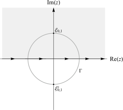
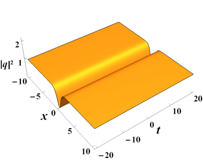
Figure 2: (a) Distribution of discrete eigenvalues $\{\xi_{0,1},\xi^{*}_{0,1}\}$; (b) A non-propagating dark soliton with $q_{+}=1$, $\xi_{0,1}=\sqrt{2}\mathrm{i}$ and $c_{0,1}=1$.

Case 5.2 $N_{1}+N_{2}=1$ ($n_{1,2}=0$, $m_{1}=0$ and $m_{2}=1$). In such case, there is one pair of pure imaginary eigenvalues $z_{0,1},\hat{z}_{0,1}$ ($|z_{0,1}|>\sqrt{2}q_{0}$) lying off the circle $\Gamma$ (see Fig. 3), so we can take $z_{0,1}=\mathrm{i}\kappa\sqrt{2}q_{0}$ with $\kappa>1$. In view of the second constraint of (3.13), the constant $d_{0,1}$ can be expressed as $d_{0,1}=-\frac{\kappa\sqrt{\kappa^{2}-1}}{\sqrt{2}\left(\kappa^{2}+1\right)}e^{\mathrm{i}\omega_{1}}$, where $\omega_{1}=\mathrm{arg}(d_{0,1})$. Thus, we obtain the dark-bright one-soliton solution as follows:

$$q(x,t) =q_{+}\Big{[}\tanh\Big{(}\frac{\sqrt{2}q_{0}}{\kappa}x\Big{)}-\frac{\sqrt{\kappa^{2}-1}}{\kappa}\mathrm{sech}\Big{(}\frac{\sqrt{2}q_{0}}{\kappa}x\Big{)}e^{\mathrm{i}\big{(}\frac{2q_{0}^{2}}{\kappa^{2}}t-\omega_{1}-2\theta_{+}\big{)}}\Big{]},$$ (5.7)

which reduces to the dark one-soliton solution (5.6) at $\kappa\to 1$. As shown in Fig. 3, the solution is heteroclinic in $x$ and periodic in $t$, so the dark and bright solitons beat each other with the period $\frac{\pi\kappa^{2}}{q_{0}^{2}}$ as $t$ evolves. Via the extreme value analysis, we find that $|q(x,t)|^{2}$ attains its maximum value $2-\frac{1}{\kappa^{2}}$ periodically at the points $\Big{(}\frac{\kappa}{\sqrt{2}q_{0}}\ln\Big{(}\frac{\sqrt{2\kappa^{2}-1}+\kappa}{\sqrt{\kappa^{2}-1}}\Big{)},\frac{\kappa^{2}(2n\pi+\omega_{1}+2\theta_{+})}{2q_{0}^{2}}\Big{)}$ and $\Big{(}\frac{\kappa}{\sqrt{2}q_{0}}\ln\Big{(}\frac{\sqrt{2\kappa^{2}-1}-\kappa}{\sqrt{\kappa^{2}-1}}\Big{)},\frac{\kappa^{2}[(2n+1)\pi+\omega_{1}+2\theta_{+}]}{2q_{0}^{2}}\Big{)}$ ($n\in\mathbb{Z}$), and it periodically drops to its minimum value $0$ at the points $\Big{(}\frac{\kappa}{\sqrt{2}q_{0}}\ln\Big{(}\frac{\sqrt{2\kappa^{2}-1}+\sqrt{\kappa^{2}-1}}{\sqrt{2}q_{0}}\Big{)},\frac{\kappa^{2}(2n\pi+\omega_{1}+2\theta_{+})}{2q_{0}^{2}}\Big{)}$ and $\Big{(}\frac{\kappa}{\sqrt{2}q_{0}}\ln\Big{(}\frac{\sqrt{2\kappa^{2}-1}-\sqrt{\kappa^{2}-1}}{\sqrt{2}q_{0}}\Big{)}$, $\frac{\kappa^{2}[(2n+1)\pi+\omega_{1}+2\theta_{+}]}{2q_{0}^{2}}\Big{)}$ ($n\in\mathbb{Z}$).

Recall that Eq. (1.2) arises from a parity-symmetric reduction of the Manakov system (1.3), where $q(x,t)$ and $q(-x,t)$ are two components of system (1.3). Thus, it is not surprising that the intensities of individual components exhibit the beating behavior [61], but their superposed intensity shows a non-propagating dark soliton, namely,

$$|q(x,t)|^{2}+|q(-x,t)|^{2} =2q^{2}_{0}\Big{(}1-\frac{1}{\kappa^{2}}\mathrm{sech}^{2}\Big{(}\frac{\sqrt{2}q_{0}}{\kappa}x\Big{)}\Big{)}.$$ (5.8)

So, solution (5.7) is also called the beating one-soliton [62] and it is neither even- or odd-symmetric with respect to $x$.

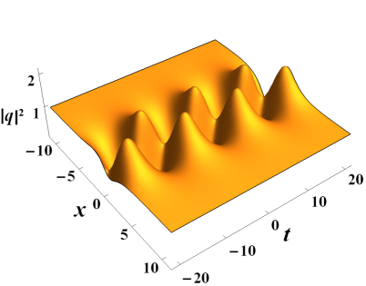
Figure 3: (a) Distribution of discrete eigenvalues $\{z_{0,1},\hat{z}_{0,1}\}$; (b) A non-propagating beating soliton with $q_{+}=e^{2\mathrm{i}}$, $z_{0,1}=2\sqrt{2}\mathrm{i}$ and $d_{0,1}=\frac{\sqrt{6}}{5}e^{3\mathrm{i}}$.

Case 5.3 $N_{1}+N_{2}=2$ ($n_{1}=1$ and $n_{2}=m_{1,2}=0$). For this case, the discrete eigenvalues appear in symmetric quartet $\{\xi_{1},-\xi_{1},\xi^{*}_{1},-\xi^{*}_{1}\}$ on the circle $\Gamma$, as shown in Fig. 4. By the relations in Eq. (3.8), the norming constants satisfy $c_{1}\overline{c}_{1}=-1$ and $\overline{c}_{1}c^{*}_{1}=1$, which means $c_{1}$ is a pure imaginary number. Then, by setting $\xi_{1}=\sqrt{2}q_{0}e^{\mathrm{i}\varsigma_{1}}$ $(\varsigma_{1}\in(0,\frac{\pi}{2}))$, we obtain the following two-soliton solution:

$$q(x,t)=q_{+}\Bigg{(}1-2\tan(\varsigma_{1})\frac{c_{1}e^{-\mathrm{i}\varsigma_{1}}e^{-2\mathrm{i}\theta_{1}(\xi_{1})}+c^{-1}_{1}e^{\mathrm{i}\varsigma_{1}}e^{-2\mathrm{i}\theta_{1}(-\xi^{*}_{1})}}{1+e^{-2\mathrm{i}\theta_{1}(\xi_{1})-2\mathrm{i}\theta_{1}(-\xi^{*}_{1})}-\mathrm{i}\sec(\varsigma_{1})\big{(}c_{1}e^{-2\mathrm{i}\theta_{1}(\xi_{1})}-c^{-1}_{1}e^{-2\mathrm{i}\theta_{1}(-\xi^{*}_{1})}\big{)}}\Bigg{)},$$ (5.9)

where

$$\theta_{1}(\xi_{1})=-\mathrm{i}\sqrt{2}q_{0}\sin(\varsigma_{1})(x+2\sqrt{2}q_{0}\cos(\varsigma_{1})t),\quad\theta_{1}(-\xi^{*}_{1})=-\mathrm{i}\sqrt{2}q_{0}\sin(\varsigma_{1})(x-2\sqrt{2}q_{0}\cos(\varsigma_{1})t).$$ (5.10)

By respectively assuming that $\mathrm{Im}[\theta_{1}(\xi_{1})]=O(1)$ and $\mathrm{Im}[\theta_{1}(-\xi^{*}_{1})]=O(1)$, we make asymptotic analysis of the solution and obtain two asymptotic solitons as $t\to\pm\infty$:

$$q^{\pm}_{\rm{I}}=q_{+}e^{\pm\mathrm{i}\varsigma_{1}}\big{[}\cos(\varsigma_{1})-\mathrm{i}\sin(\varsigma_{1})\tanh(\eta_{\rm{I}}^{\pm})\big{]},$$ (5.11a)

$$q^{\pm}_{\rm{I\!I}}=q_{+}e^{\pm\mathrm{i}\varsigma_{1}}\big{[}\cos(\varsigma_{1})+\mathrm{i}\sin(\varsigma_{1})\tanh(\eta_{\rm{I\!I}}^{\pm})\big{]},$$ (5.11b)

where

$$\eta^{\pm}_{\rm{I}}=\sqrt{2}q_{0}\sin(\varsigma_{1})[x-2\sqrt{2}q_{0}\cos(\varsigma_{1})t]\mp\frac{1}{2}\ln\Bigg{(}\frac{|c_{1}|^{\mp 1}}{\cos(\varsigma_{1})}\Bigg{)},$$

$$\eta^{\pm}_{\rm{I\!I}}=\sqrt{2}q_{0}\sin(\varsigma_{1})[x+2\sqrt{2}q_{0}\cos(\varsigma_{1})t]\pm\frac{1}{2}\ln\Bigg{(}\frac{|c_{1}|^{\mp 1}}{\cos(\varsigma_{1})}\Bigg{)}.$$

Apparently, both the asymptotic expressions $q^{\pm}_{\rm{I}}$ and $q^{\pm}_{\rm{I\!I}}$ have no singularity, and they can describe two gray solitons with the velocities $v^{\pm}_{\rm{I}}=-v^{\pm}_{\rm{I\!I}}=2\sqrt{2}q_{0}\cos(\varsigma_{1})$ (see Fig. 4). Based on the expressions of asymptotic solitons, the extreme values of $|q^{\pm}_{\rm{I}}|^{2}$ and $|q^{\pm}_{\rm{I\!I}}|^{2}$ can be obtained as

$$A_{\rm{I}}^{\pm}=A_{\rm{I\!I}}^{\pm}=q_{0}^{2}\cos^{2}(\varsigma_{1}),$$

where $\sin(\varsigma_{1})$ characterizes the darkness of soliton. The soliton position shifts between $q_{\rm{I},\rm{I\!I}}^{+}$ and $q_{\rm{I},\rm{I\!I}}^{-}$ are, respectively, given by $\Delta x_{0,\rm{I}}=\frac{\ln(\cos(\varsigma_{1}))}{\sqrt{2}q_{0}\sin(\varsigma_{1})},\Delta x_{0,\rm{I\!I}}=-\frac{\ln(\cos(\varsigma_{1}))}{\sqrt{2}q_{0}\sin(\varsigma_{1})}$, and their phase shift are $\Delta\phi_{\rm{I}}=\Delta\phi_{\rm{I\!I}}=2\varsigma_{1}$.

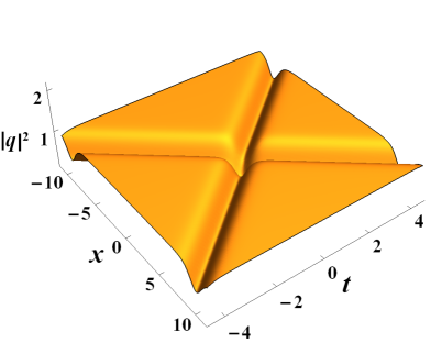
Figure 4: (a) Distribution of discrete eigenvalues $\{\xi_{1},-\xi_{1},\xi^{*}_{1},-\xi^{*}_{1}\}$; (b) An interaction between two propagating dark solitons with $q_{+}=1$, $\xi_{1}=\sqrt{2}e^{\mathrm{i}\frac{\pi}{4}}$ and $c_{1}=2\mathrm{i}$.

Case 5.4 $N_{1}+N_{2}=2$ ($n_{2}=1$ and $n_{1}=m_{1,2}=0$). In this case, the discrete eigenvalues appear in symmetric quartet $\{z_{1},-z^{*}_{1},\hat{z}_{1},-\hat{z}^{*}_{1}\}$ off the circle $\Gamma$, as shown in Fig. 5. Correspondingly, the norming constants satisfy the constraints in (3.11) and the eigenvalue $z_{1}$ can be taken as $z_{1}=\sqrt{2}\kappa q_{0}e^{\mathrm{i}\varsigma_{1}}$, where $\varsigma_{1}\in(0,\frac{\pi}{2})$ and $\kappa>1$ (Note that for $0<\kappa<1$ the denominator always crosses zeros, which implies that the solutions have singularities). At the same time, one should notice that there exist the following relations:

$$\theta_{2}(z)-\theta_{1}(z)=\theta_{1}(\hat{z})+\theta_{2}(\hat{z}),$$ (5.12a)

$$\theta_{2}(z_{1})-\theta_{1}(z_{1})=\frac{q_{0}}{\kappa^{2}}\Big{[}-\big{(}\sqrt{2}\kappa\cos(\varsigma_{1})x+2q_{0}\cos(2\varsigma_{1})t\big{)}+\mathrm{i}\sin(\varsigma_{1})\big{(}\sqrt{2}\kappa x+4q_{0}\cos(\varsigma_{1})t\big{)}\Big{]},$$ (5.12b)

$$\theta_{2}(-z^{*}_{1})-\theta_{1}(-z^{*}_{1})=\frac{q_{0}}{\kappa^{2}}\Big{[}\big{(}\sqrt{2}\kappa\cos(\varsigma_{1})x-2q_{0}\cos(2\varsigma_{1})t\big{)}+\mathrm{i}\sin(\varsigma_{1})\big{(}\sqrt{2}\kappa x-4q_{0}\cos(\varsigma_{1})t\big{)}\Big{]}.$$ (5.12c)

By respectively assuming that $\mathrm{Im}[\theta_{2}(z_{1})-\theta_{1}(z_{1})]=O(1)$ and $\mathrm{Im}[\theta_{2}(-z^{*}_{1})-\theta_{1}(-z^{*}_{1})]=O(1)$, the asymptotic analysis shows that there are two asymptotic solitons as $t\to\pm\infty$:

$$q^{\pm}_{\rm{I}}=q_{+}e^{\pm\mathrm{i}\varsigma_{1}}\Big{[}\cos(\varsigma_{1})-\mathrm{i}\sin(\varsigma_{1})\tanh(\eta^{\pm}_{\rm{I}})-\tau_{1}^{\pm}\mathrm{sech}(\eta^{\pm}_{\rm{I}})e^{\mathrm{i}\varpi^{\pm}_{\rm{I}}}\Big{]},$$ (5.13a)

$$q^{\pm}_{\rm{I\!I}}=q_{+}e^{\pm\mathrm{i}\varsigma_{1}}\Big{[}\cos(\varsigma_{1})+\mathrm{i}\sin(\varsigma_{1})\tanh(\eta^{\pm}_{\rm{I\!I}})+\tau_{1}^{\pm}\mathrm{sech}(\eta^{\pm}_{\rm{I\!I}})e^{\mathrm{i}\varpi^{\pm}_{\rm{I\!I}}}\Big{]},$$ (5.13b)

with

$$\eta^{\pm}_{\rm{I}}=\frac{q_{0}\sin(\varsigma_{1})}{\kappa^{2}}[\sqrt{2}\kappa x-4q_{0}\cos(\varsigma_{1})t]+\frac{1}{2}\ln(\nu_{1}^{\pm}),\quad\varpi^{\pm}_{\rm{I}}=\frac{q_{0}}{\kappa^{2}}[\sqrt{2}\kappa\cos(\varsigma_{1})x-2q_{0}\cos(2\varsigma_{1})t]\mp\varsigma_{1}$$

$$\eta^{\pm}_{\rm{I\!I}}=\frac{q_{0}\sin(\varsigma_{1})}{\kappa^{2}}[\sqrt{2}\kappa x+4q_{0}\cos(\varsigma_{1})t]-\frac{1}{2}\ln(\nu_{1}^{\pm}),\quad\varpi^{\pm}_{\rm{I\!I}}=-\frac{q_{0}}{\kappa^{2}}[\sqrt{2}\kappa\cos(\varsigma_{1})x+2q_{0}\cos(2\varsigma_{1})t]\mp\varsigma_{1},$$

$$\nu_{1}^{+}=\frac{\kappa^{2}\cos^{2}(\varsigma_{1})}{\kappa^{4}-2\kappa^{2}\cos(2\varsigma_{1})+1}\frac{\kappa^{2}-1}{2|d_{1}|^{2}},\quad\nu_{1}^{-}=\frac{\kappa^{4}+2\kappa^{2}\cos(2\varsigma_{1})+1}{\cos^{4}(\varsigma_{1})(\kappa^{2}+1)^{2}}\nu_{1}^{+},$$

$$\tau_{1}^{+}=\frac{d^{*}_{1}}{|d_{1}|}\frac{\sqrt{\kappa^{2}-1}}{\kappa}\frac{\mathrm{i}e^{-2\mathrm{i}\theta_{+}}\sin(\varsigma_{1})(e^{2\mathrm{i}\varsigma_{1}}-\kappa^{2})}{\sqrt{\kappa^{4}-2\kappa^{2}\cos(2\varsigma_{1})+1}},\quad\tau_{1}^{-}=\frac{\sqrt{\kappa^{4}+2\kappa^{2}\cos(2\varsigma_{1})+1}}{\kappa^{2}+e^{2\mathrm{i}\varsigma_{1}}}\tau_{1}^{+}.$$

It can be seen from Eqs. (5.13a) and (5.13b) that both the asymptotic expressions $q^{\pm}_{\rm{I}}$ and $q^{\pm}_{\rm{I\!I}}$ are non-singular, and they can describe two propagating beating solitons with the same $t$-period $\frac{\pi\kappa^{2}}{q^{2}_{0}\cos(2\varsigma_{1})}$ and same $x$-period $\frac{\sqrt{2}\pi\kappa}{q_{0}\cos(\varsigma_{1})}$ (see Fig. 5).

Besides, for the special case that $z_{1},\hat{z}_{1}$ merges into an eigenvalue $\xi_{1}=\sqrt{2}q_{0}e^{\mathrm{i}\varsigma_{1}}$ on $\Gamma$, Eq. (3.16) says that $\displaystyle\lim_{\kappa\to 1}\frac{\kappa^{2}-1}{|d_{1}|^{2}}=8|c_{1}|\sin(\varsigma_{1})\tan(\varsigma_{1})$, $\displaystyle\lim_{\kappa\to 1}\tau_{1}^{\pm}=0$ and $\displaystyle\lim_{\kappa\to 1}\nu_{1}^{\pm}=|c_{1}|\cos^{\pm 1}(\varsigma_{1})$, where $c_{1}$ is the norming constant corresponding to $\xi_{1}$. Hence, $q^{\pm}_{\rm{I}}$ and $q^{\pm}_{\rm{I\!I}}$ can be reduced to the asymptotic solitons (5.11a) and (5.11b) at $\kappa\to 1$.

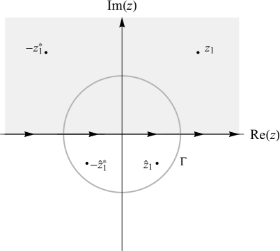
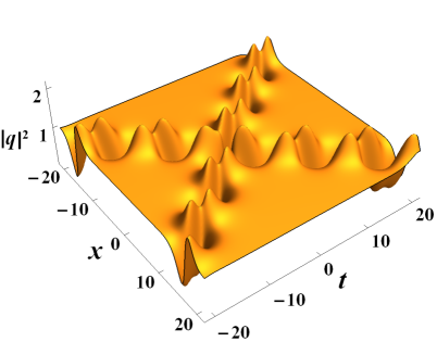
Figure 5: (a) Distribution of discrete eigenvalues $\{z_{1},\hat{z}_{1},-z^{*}_{1},-\hat{z}^{*}_{1}\}$; (b) An interaction between two propagating beating solitons with $q_{+}=1$, $z_{1}=\sqrt{5}e^{\mathrm{i}\arctan(2)}$ and $d_{1}=1$.

Case 5.5 $N_{1}+N_{2}=2$ ($m_{2}=2,\,n_{1,2}=m_{1}=0$ and $m_{1,2}=1,\,n_{1,2}=0$). In both the two subcases, all the four discrete eigenvalues are pure imaginary numbers. (i) For the first subcase, the distribution of two pairs of eigenvalues $\{z_{0,1},\hat{z}_{0,1}\}$ and $\{z_{0,2},\hat{z}_{0,2}\}$ is shown in Fig. 6. Because of their being off the circle $\Gamma$, the eigenvalue pairs lead to two beating solitons which are both homoclinic in $x$ but have different periods in $t$. Such two beating solitons are non-propagating and are linearly superposed around $x=O(1)$, as seen in Fig. 6. (ii) For the second subcase, there are one pair of imaginary eigenvalues $\{z_{0,1},\hat{z}_{0,1}\}$ off the circle $\Gamma$ and another pair of imaginary eigenvalues $\{\xi_{0,1},\xi^{*}_{0,1}\}$ on $\Gamma$ (see Fig. 6). Fig. 6 shows the superimposition of one beating soliton and one dark soliton around $x=O(1)$.

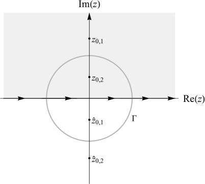
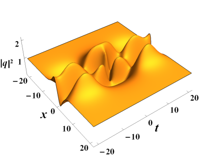
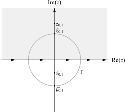
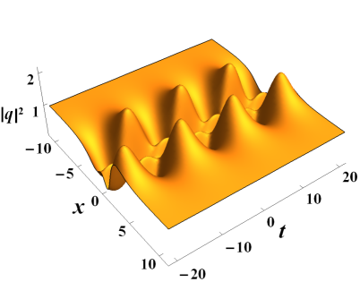
Figure 6: (a) Distribution of discrete eigenvalues $\{z_{0,1},z_{0,2},\hat{z}_{0,1},\hat{z}_{0,2}\}$; (b) Superposition of two non-propagating beating solitons with $q_{+}=1$, $z_{0,1}=2\sqrt{2}\mathrm{i}$, $z_{0,2}=3\sqrt{2}\mathrm{i}$, $d_{0,1}=\sqrt{\frac{6}{35}}$ and $d_{0,2}=\frac{\sqrt{3}}{5}$; (c) Distribution of discrete eigenvalues $\{\xi_{0,1},\xi^{*}_{0,1},z_{0,1},\hat{z}_{0,1}\}$; (d) Superposition of non-propagating beating soliton and dark soliton with $q_{+}=1$, $\xi_{0,1}=\sqrt{2}\mathrm{i}$, $z_{0,1}=2\sqrt{2}\mathrm{i}$, $c_{0,1}=1$ and $d_{0,1}=\frac{\sqrt{2}}{5}$.

6 Conclusions

For the defocusing local-and-nonlocal NLS equation (1.2) with NZBC, we have developed the theory of IST by using the Riemann-Hilbert method. Similar to the Manakov system, we have introduced the adjoint Lax pair and auxiliary eigenfunctions for the direct scattering problem, and studied the analyticity, symmetries and asymptotic behaviors of the Jost eigenfunctions, auxiliary Jost eigenfunctions and scattering coefficients. Then, we have regularized a RHP for the inverse problem, analyzed the residue conditions at the discrete eigenvalues, and obtained the integral representation for the solutions. It is worth noting that the Manakov system (1.3) with NZBC admits two symmetries, while Eq. (1.2) with NZBC has one more symmetry due to the presence of the nonlocality. This additional symmetry leads to some stricter constraints on the scattering coefficients, eigenfunctions and norming constants. In particular, we have studied the properties of the Jost eigenfunctions and auxiliary Jost eigenfunctions when the discrete eigenvalues are on/off the circle $\Gamma$, and explicitly obtained the associated constraints on norming constants. We point that it is also essential to introduce an adjoint Lax pair for the IST theory of the focusing Eq. (1.2) with NZBC, and the analyticity must be examined in four domains, analogous to the focusing Manakov system studied in Ref. [63].

On the other hand, we have presented the N-soliton solutions in the determinant form for the reflectionless case. If the asymptotic phase difference $\theta_{+}-\theta_{-}=\pi$ ($q_{+}=-q_{-}$), the number of pure imaginary eigenvalues must be odd; whereas if $\theta_{+}-\theta_{-}=0$ ($q_{+}=q_{-}$) the number of pure imaginary eigenvalues must be even. Also, we have discussed the soliton dynamical behavior based on the distribution of discrete eigenvalues and the asymptotic behavior of solutions. It has been found that the discrete eigenvalue pairs lying on and off the circle $\Gamma$, respectively, lead to the dark and beating solitons. Moreover, our analysis has demonstrated that the two-soliton solutions can manifest diverse interaction patterns, including the interactions between two dark solitons or two beating solitons, as well as the superpositions of two beating solitons or one beating soliton and one dark soliton. This rich variety of soliton interactions stems from the possibility of different distribution of discrete eigenvalue pairs in the spectrum plane. In addition, we emphasize that the admissible solutions of Eq. (1.1) are not necessarily even- or odd-symmetric with respect to $x$ (e.g., the beating one-soliton solution (5.7)), despite the invariance of this equation under the transformation $q(x,t)\to q(-x,t)$.

Authors Contributions

Chuanxin Xu: Conceptualization; Formal analysis; Software; Writing Coriginal draft. Tao Xu: Conceptualization; Formal analysis; Validation; Writing Coriginal draft; Funding acquisition. Min Li: Formal analysis; Validation; Writing Creview & editing; Funding acquisition.

Appendix Appendix A

A.1 Proof of Theorem 2.1

For brevity, we omit the dependence on $t$. Based on the relation (2.17), Eq. (2.16a) can be rewritten as

$$\bm{\mu}_{-}(x,z)=\mathbf{Y}_{-}(z)\bigg{[}\mathrm{I}+\int_{-\infty}^{x}e^{\mathrm{i}\mathbf{J}(z)(x-y)}\mathbf{Y}^{-1}_{-}(z)\bm{\Delta}\!\mathbf{Q}_{-}(y)\bm{\mu}_{-}(y,z)e^{\mathrm{i}\mathbf{J}(z)(y-x)}dy\bigg{]}.$$ (A.1)

By denoting the first column of $\mathbf{Y}^{-1}_{-}(z)\bm{\mu}_{-}(x,z)$ as $\chi(x,z)$, we have

$$\chi(x,z)=\left(\begin{array}[]{ccc}1\\ 0\\ 0\\ \end{array}\right)+\int_{-\infty}^{x}\mathbf{G}(x-y,z)\bm{\Delta}\!\mathbf{Q}_{-}(y)\mathbf{Y}_{-}(z)\chi(y,z)dy,$$ (A.2)

with

$$\mathbf{G}(x-y,z)=\mathrm{diag}\big{(}1,e^{\mathrm{i}(\lambda-k)(x-y)},e^{2\mathrm{i}\lambda(x-y)}\big{)}\mathbf{Y}^{-1}_{-}(z).$$ (A.3)

Then, we represent $\chi(x,z)$ in the Neumann series:

$$\chi(x,z)=\sum_{n=0}^{\infty}\chi^{(n)}(x,z),$$ (A.4)

with

$$\chi^{(0)}(x,z)=\left(\begin{array}[]{ccc}1\\ 0\\ 0\\ \end{array}\right),\quad\chi^{(n+1)}(x,z)=\int_{-\infty}^{x}\mathbf{\Upsilon}(x,y,z)\chi^{(n)}(y,z)dy,$$ (A.5)

where $\mathbf{\Upsilon}(x,y,z)=\mathbf{G}(x-y,z)\bm{\Delta}\!\mathbf{Q}_{-}(y)\mathbf{Y}_{-}(z)$.

Introducing the $L^{1}$ vector norm $||\chi(x,z)||=|\chi_{1}|+|\chi_{2}|+|\chi_{3}|$ and the corresponding subordinate matrix norm $||\mathbf{\Upsilon}(x,y,z)||$ yields

$$\parallel\chi^{(n+1)}(x,z)\parallel\leq\int_{-\infty}^{x}\parallel\mathbf{\Upsilon}(x,y,z)\parallel\,\parallel\chi^{(n)}(y,z)\parallel dy.$$ (A.6)

Note that $\parallel\mathbf{Y}_{-}(z)\parallel<2+\frac{2\sqrt{2}q_{0}}{|z|}$ and $\parallel\mathbf{Y}^{-1}_{-}(z)\parallel<\big{(}\sqrt{2}+\frac{2q_{0}}{|z|}\big{)}/|\gamma(z)|+\frac{\sqrt{2}}{2}$, where $\gamma(z)=2-\frac{4q^{2}_{0}}{z^{2}}$. The properties of matrix norm imply that

$$\parallel\mathbf{\Upsilon}(x,y,z)\parallel \leq\parallel\mathrm{diag}(1,e^{\mathrm{i}(\lambda-k)(x-y)},e^{2\mathrm{i}\lambda(x-y)})\parallel\,\parallel\mathbf{Y}^{-1}_{-}(z)\parallel\,\parallel\bm{\Delta}\!\mathbf{Q}_{-}(y)\parallel\,\parallel\mathbf{Y}_{-}(z)\parallel$$ (A.7)

$$\leq c(z)(1+e^{-(\lambda_{\mathrm{I}}-k_{\mathrm{I}})(x-y)}+e^{-2\lambda_{\mathrm{I}}(x-y)})\parallel\bm{\Delta}\!\mathbf{Q}_{-}(y)\parallel.$$

where $\lambda_{\mathrm{I}}=\mathrm{Im}(\lambda)$, $k_{\mathrm{I}}=\mathrm{Im}(k)$, and $c(z)=\frac{\sqrt{2}(|z|^{2}+\sqrt{2}q_{0})^{2}}{|z^{2}-2q^{2}_{0}|}+\sqrt{2}+\frac{2q_{0}}{|z|}$. On the other hand, $c(z)\to\infty$ as $z\to 0$ or $z\to\pm\sqrt{2}q_{0}$. Thus, for any given $\epsilon>0$, we consider the domain $(C^{+})_{\epsilon}=C^{+}\setminus\big{(}B_{\epsilon}(0)\cup B_{\epsilon}(\sqrt{2}q_{0})\cup B_{\epsilon}(-\sqrt{2}q_{0})\big{)}$, where $B_{\epsilon}(z_{0})=\{z\in\mathbb{C}:|z-z_{0}|<\epsilon q_{0}\}$. It is straightforward to show that $c_{\epsilon}=\displaystyle\mathrm{max}_{z\in(C^{+})_{\epsilon}}c(z)<\infty$.

Next, we use the inductive method to prove that the following inequality holds for all $z\in(C^{+})_{\epsilon}$ and for all $n\in\mathbb{N}$:

$$\parallel\chi^{(n)}(x,z)\parallel\leq\frac{M^{n}(x)}{n!},$$ (A.8)

where

$$M(x)=3c_{\epsilon}\int_{-\infty}^{x}\parallel\bm{\Delta}\!\mathbf{Q}_{-}(y)\parallel dy.$$ (A.9)

The claim is naturally true for $n=0$, and one has $1+e^{-(\lambda_{\mathrm{I}}-k_{\mathrm{I}})(x-y)}+e^{-2\lambda_{\mathrm{I}}(x-y)}\leq 3$ for all $z\in(C^{+})_{\epsilon}$ and for all $y\leq x$. Assuming that (A.8) holds at $n=j$, it follows from (A.6) that

$$\parallel\chi^{(j+1)}(x,z)\parallel\leq\frac{3c_{\epsilon}}{j!}\int_{-\infty}^{x}\parallel\bm{\Delta}\!\mathbf{Q}_{-}(y)\parallel M^{j}(y)dy=\frac{M^{j+1}(x)}{(j+1)!},$$ (A.10)

which proves the induction step. That is, if $\parallel\bm{\Delta}\!\mathbf{Q}_{-}(x)\parallel\in L^{1}(\mathbb{R})$, the Neumann series converges absolutely for $z\in(C^{+})_{\epsilon}$. Therefore, we know that $\mu_{-,1}$ is analytic for $z\in C^{+}$ since a uniformly convergent series of analytic function converges to an analytic function and $\epsilon$ is arbitrary.

Similarly, one can prove the analyticity of $\mu_{+,3}(x,t,z)$ in $C^{+}$ and $\mu_{+,1}(x,t,z),\mu_{-,3}(x,t,z)$ in $C^{-}$.

A.2 Analyticity of scattering coefficients

By virtue of Eq. (2.5a), we have

$$[\bm{\phi}^{-1}(x,t,z)]_{x}=-\bm{\phi}^{-1}(x,t,z)(\mathbf{X}_{\pm}(z)+\bm{\Delta}\!\mathbf{Q}_{\pm}(x,t)),$$ (A.11)

$$[\bm{\phi}^{-1}(x,t,z)]_{t}=-\bm{\phi}^{-1}(x,t,z)(\mathbf{T}_{\pm}(z)+\bm{\Delta}\!\mathbf{T}_{\pm}(x,t)).$$

Then, inserting the relation (2.17) into Eq. (A.11) gives rise to

$$[\bm{\mu}^{-1}_{\pm}(x,t,z)\mathbf{Y}_{\pm}(z)]_{x}+\mathrm{i}[\bm{\mu}^{-1}_{\pm}(x,t,z)\mathbf{Y}_{\pm}(z),\mathbf{J}(z)]=-\bm{\mu}^{-1}_{\pm}(x,t,z)\bm{\Delta}\!\mathbf{Q}_{\pm}(x,t)\mathbf{Y}_{\pm}(z),$$ (A.12)

$$[\bm{\mu}^{-1}_{\pm}(x,t,z)\mathbf{Y}_{\pm}(z)]_{t}+\mathrm{i}[\bm{\mu}^{-1}_{\pm}(x,t,z)\mathbf{Y}_{\pm}(z),\mathbf{\Omega}(z)]=-\bm{\mu}^{-1}_{\pm}(x,t,z)\bm{\Delta}\!\mathbf{T}_{\pm}(x,t)\mathbf{Y}_{\pm}(z).$$

Based on Eq. (A.12), we can obtain the total differential form

$$-d\big{(}\mathbf{E}^{-1}(x,t,z)\bm{\mu}^{-1}_{\pm}(x,t,z)\mathbf{Y}_{\pm}(z)\mathbf{E}(x,t,z)\big{)}$$

$$\hskip 56.9055pt=\big{(}\mathbf{E}^{-1}(x,t,z)\bm{\mu}^{-1}_{\pm}(x,t,z)\bm{\Delta}\!\mathbf{Q}_{\pm}(x,t)\mathbf{Y}_{\pm}(z)\mathbf{E}(x,t,z)\big{)}dx$$

$$\hskip 68.28644pt+\big{(}\mathbf{E}^{-1}(x,t,z)\bm{\mu}^{-1}_{\pm}(x,t,z)\bm{\Delta}\!\mathbf{T}_{\pm}(x,t)\mathbf{Y}_{\pm}(z)\mathbf{E}(x,t,z)\big{)}dt.$$ (A.13)

Thus, choosing the integration paths $(x,t)\to(\infty,t)$ and $(-\infty,t)\to(x,t)$, $\bm{\mu}^{-1}_{\pm}(x,t,z)$ can be represented as the Volterra integral equations:

$$\bm{\mu}^{-1}_{+}(x,t,z)=\mathbf{Y}^{-1}_{+}(z)+\int_{x}^{\infty}e^{\mathrm{i}\mathbf{J}(z)(x-y)}\bm{\mu}^{-1}_{+}(y,t,z)\bm{\Delta}\!\mathbf{Q}_{+}(y,t)\mathbf{Y}_{+}(z)\bm{\mu}^{-1}_{+}(y,t,z)e^{-\mathrm{i}\mathbf{J}(z)(x-y)}\mathbf{Y}^{-1}_{+}(z)dy,$$

$$\bm{\mu}^{-1}_{-}(x,t,z)=\mathbf{Y}^{-1}_{-}(z)-\int_{-\infty}^{x}e^{\mathrm{i}\mathbf{J}(z)(x-y)}\bm{\mu}^{-1}_{-}(y,t,z)\bm{\Delta}\!\mathbf{Q}_{-}(y,t)\mathbf{Y}_{-}(z)\bm{\mu}^{-1}_{-}(y,t,z)e^{-\mathrm{i}\mathbf{J}(z)(x-y)}\mathbf{Y}^{-1}_{-}(z)dy.$$

Using the same way in Appendix A.1, we can prove that $[\bm{\mu}^{-1}_{+}]^{1}(x,t,z)$ and $[\bm{\mu}^{-1}_{-}]^{3}(x,t,z)$ are analytic in $C^{-}$, $[\bm{\mu}^{-1}_{-}]^{1}(x,t,z)$ and $[\bm{\mu}^{-1}_{+}]^{3}(x,t,z)$ are analytic in $C^{+}$, and $[\bm{\mu}^{-1}_{\pm}]^{2}(x,t,z)$ are nowhere analytic, where $[\bm{\mu}^{-1}_{\pm}]^{j}$ represent the $j$th rows of $\bm{\mu}^{-1}_{\pm}$. Based on the relation (2.17), the corresponding rows of $\bm{\phi}^{-1}_{\pm}$ have the same analyticity. Then, by the relations $\mathbf{A}(z)=\bm{\phi}^{-1}_{+}(x,t,z)\bm{\phi}_{-}(x,t,z)$ and $\mathbf{B}(z)=\bm{\phi}^{-1}_{-}(x,t,z)\bm{\phi}_{+}(x,t,z)$, Theorem 2.2 can be finally proved.

A.3 Adjoint problem

Proof of Proposition 2.4: We suppress the $x$-, $t$- and $z$-dependence for brevity. For any two column vectors $u,v\in\mathbb{C}^{3}$, there are the following identities:

$$(\bm{\sigma}_{3}u)\times(\bm{\sigma}_{3}v)+\bm{\sigma}_{3}(u\times v)=\mathbf{0},$$ (A.14a)

$$(\bm{\sigma}_{3}u)\times v+u\times(\bm{\sigma}_{3}v)-u\times v-(\bm{\sigma}_{3}u)\times(\bm{\sigma}_{3}v)=\mathbf{0},$$ (A.14b)

$$(\mathbf{Q}^{*}u)\times v+u\times(\mathbf{Q}^{*}v)-\bm{\sigma}_{3}\mathbf{Q}\bm{\sigma}_{3}(u\times v)=\mathbf{0},$$ (A.14c)

$$(\bm{\sigma}_{3}\mathbf{Q}^{*}_{x}u)\times u+u\times(\bm{\sigma}_{3}\mathbf{Q}^{*}_{x}v)=-\mathbf{Q}_{x}\bm{\sigma}_{3}(u\times v),$$ (A.14d)

$$(\bm{\sigma}_{3}(\mathbf{Q}^{*})^{2}u)\times u+u\times(\bm{\sigma}_{3}(\mathbf{Q}^{*})^{2}v)=-\mathbf{Q}^{2}\bm{\sigma}_{3}(u\times v),$$ (A.14e)

$$2\mathrm{i}q^{2}_{0}(u\times v)+(\mathbf{V}_{0}u)\times v+u\times(\mathbf{V}_{0}v)=-\bm{\sigma}_{3}\mathbf{V}_{0}\bm{\sigma}_{3}(u\times v),$$ (A.14f)

where ’$\times$’ represents the usual cross product. These identities will be used in the following process.

$$r_{x}=e^{\mathrm{i}\theta_{2}}\bm{\sigma}_{3}\big{\{}-\mathrm{i}k\big{[}u\times v-(\bm{\sigma}_{3}u)\times v-u\times(\bm{\sigma}_{3}v)\big{]}+(\mathbf{Q}^{*}u)\times v+u\times(\mathbf{Q}^{*}v)\big{\}},$$ (A.15a)

$$r_{t}=2kr_{x}+e^{\mathrm{i}\theta_{2}}\bm{\sigma}_{3}\big{\{}\big{[}2\mathrm{i}q^{2}_{0}(u\times v)+(\mathbf{V}_{0}u)\times v+u\times(\mathbf{V}_{0}v)\big{]}-\mathrm{i}\big{[}(\bm{\sigma}_{3}\mathbf{Q}^{*}_{x}u)\times v+u\times(\bm{\sigma}_{3}\mathbf{Q}^{*}_{x}v)\big{]}$$

$$\hskip 81.09052pt+\mathrm{i}\big{[}(\bm{\sigma}_{3}(\mathbf{Q}^{*})^{2}u)\times v+u\times(\bm{\sigma}_{3}(\mathbf{Q}^{*})^{2}v)\big{]}\big{\}}.$$ (A.15b)

Applying the relations (A.14a)-(A.14c) to Eq. (A.15a), and the relations (A.14d)-(A.14f) to Eq. (A.15b), we can obtain

$$r_{x} =e^{\mathrm{i}\theta_{2}}\bm{\sigma}_{3}\big{[}-\mathrm{i}k\bm{\sigma}_{3}(u\times v)+\bm{\sigma}_{3}\mathbf{Q}\bm{\sigma}_{3}(u\times v)\big{]}=(-\mathrm{i}k\bm{\sigma}_{3}+\mathbf{Q})r,$$ (A.16a)

$$r_{t} =2k\mathbf{X}r+e^{\mathrm{i}\theta_{2}}\bm{\sigma}_{3}\big{(}-\bm{\sigma}_{3}\mathbf{V}_{0}\bm{\sigma}_{3}(u\times v)+\mathrm{i}\mathbf{Q}_{x}\bm{\sigma}_{3}(u\times v)-\mathrm{i}\mathbf{Q}^{2}\bm{\sigma}_{3}(u\times v)\big{)}$$

$$=\big{(}2k\mathbf{X}+\mathrm{i}\bm{\sigma}_{3}\mathbf{Q}_{x}-\mathrm{i}\bm{\sigma}_{3}\mathbf{Q}^{2}-\mathbf{V}_{0}\big{)}r,$$ (A.16b)

which indicates that $r$ is a solution of Lax pair (2.5).

Proof of Lemma 2.5: To illustrate, we only verify Eq. (2.35a) at $j=2$ (which means that $l=3,m=1$) since the other cases can be proved similarly. Based on Eqs. (LABEL:4) and (2.32), we know that the functions $v_{\pm}(x,t)=e^{\mathrm{i}\theta_{2}}\bm{\sigma}_{3}\big{[}\tilde{\phi}_{\pm,3}\times\tilde{\phi}_{\pm,1}\big{]}$ satisfy the Lax pair (2.5) and exhibit the asymptotic behavior

$$v_{\pm}(x,t,z)\sim\gamma(z)e^{\mathrm{i}\theta_{2}(x,t,z)}\mathbf{Y}_{\pm,3}(z)+o(1),\quad x\to\pm\infty.$$ (A.17)

On the other hand, $v_{\pm}$ can be represented as a linear combination of the columns of $\phi_{\pm}$, i.e.,

$$v_{\pm}(x,t,z)=a_{\pm}(z)\phi_{\pm,1}(x,t,z)+b_{\pm}(z)\phi_{\pm,2}(x,t,z)+c_{\pm}(z)\phi_{\pm,3}(x,t,z).$$ (A.18)

Then, by requiring Eq. (A.18) satisfy the asymptotic behavior in Eq. (A.17), it can be determined that $a_{\pm}(z)=c_{\pm}(z)=0,b_{\pm}(z)=\gamma(z)$.

Proof of Lemma 2.6: For brevity, we suppress $x$-, $t$-, and $z$- dependence again. Substituting Eq. (2.35b) into Eq. (2.29) yields

$$(\phi_{-,2}\times\phi_{-,3},\,\phi_{-,3}\times\phi_{-,1},\,\phi_{-,1}\times\phi_{-,2})\bm{\Xi}^{-1}$$

$$\quad\quad=(\phi_{+,2}\times\phi_{+,3},\,\phi_{+,3}\times\phi_{+,1},\,\phi_{+,1}\times\phi_{+,2})\bm{\Xi}^{-1}\tilde{\mathbf{A}}.$$

Note that the following relation holds

$$(\mathbf{A}^{T})^{-1}=\frac{1}{\mathrm{det}(\mathbf{A})}(A_{2}\times A_{3},\,A_{3}\times A_{1},\,A_{1}\times A_{2}),$$ (A.19)

where $A_{i}$ is the $i$th column of $\mathbf{A}$. Then, applying this relation to Eq. (A.3) gives rise to

$$\mathrm{det}(\bm{\phi}_{-})(\bm{\phi}^{T}_{-})^{-1}\bm{\Xi}^{-1}=\mathrm{det}(\bm{\phi}_{+})(\bm{\phi}^{T}_{+})^{-1}\bm{\Xi}^{-1}\tilde{\mathbf{A}},$$ (A.20)

which, by virtue of Eq. (2.22), can be converted into

$$\bm{\Xi}(\mathbf{A}^{-1})^{T}\bm{\Xi}^{-1}=\tilde{\mathbf{A}}.$$ (A.21)

Proof of Proposition 2.7: Based on Eq. (2.29), the functions $w(x,t,z)$ and $\overline{w}(x,t,z)$ in Eq. (2.33) can be written as

$$w(x,t,z) =e^{\mathrm{i}\theta_{2}}\bm{\sigma}_{3}\big{[}\tilde{a}_{23}(z)\tilde{\phi}_{+,2}(x,t,z)\times\tilde{\phi}_{+,1}(x,t,z)+\tilde{a}_{33}(z)\tilde{\phi}_{+,3}(x,t,z)\times\tilde{\phi}_{+,1}(x,t,z)\big{]}/\gamma(z),$$ (A.22)

$$\overline{w}(x,t,z) =e^{\mathrm{i}\theta_{2}}\bm{\sigma}_{3}\big{[}\tilde{a}_{11}(z)\tilde{\phi}_{+,1}(x,t,z)\times\tilde{\phi}_{+,3}(x,t,z)+\tilde{a}_{21}(z)\tilde{\phi}_{+,2}(x,t,z)\times\tilde{\phi}_{+,3}(x,t,z)\big{]}/\gamma(z).$$

Then, replacing the cross products in the above equations by virtue of Eq. (2.35) yields

$$w(x,t,z) =\big{[}\tilde{a}_{23}(z)\phi_{+,3}(x,t,z)+\tilde{a}_{33}(z)\gamma(z)\phi_{+,2}(x,t,z)\big{]}/\gamma(z),$$ (A.23)

$$\overline{w}(x,t,z) =\big{[}-\tilde{a}_{11}(z)\gamma(z)\phi_{+,2}(x,t,z)+\tilde{a}_{21}(z)\phi_{+,1}(x,t,z)\big{]}/\gamma(z).$$

Meanwhile, noticing from Lemma 2.6 that $\tilde{a}_{32}(z)=-\gamma(z)b_{32}(z)$, $\tilde{a}_{33}(z)=b_{33}(z)$, $\tilde{a}_{21}(z)=\gamma(z)b_{12}(z)$, $\tilde{a}_{11}(z)=b_{11}(z)$, thus we obtain

$$w(x,t,z) =-b_{32}(z)\phi_{+,3}(x,t,z)+b_{33}(z)\phi_{+,2}(x,t,z),$$ (A.24)

$$\overline{w}(x,t,z) =-b_{11}(z)\phi_{+,2}(x,t,z)+b_{12}(z)\phi_{+,1}(x,t,z),$$

which indicates that Eq. (2.38a) holds true. Similarly, one can prove the validity of Eq. (2.38b) by combining Eqs. (2.33) and $\tilde{\bm{\phi}}_{+}(x,t,z)=\tilde{\bm{\phi}}_{-}(x,t,z)\tilde{\mathbf{B}}(z)$.

A.4 Symmetry

Proof of Lemma 2.8: Here, the $x$-, and $t$-dependence is suppressed for brevity. Taking the derivatives of $\bm{\sigma}_{3}(\bm{\phi}^{\dagger}(z^{*}))^{-1}$, respectively, with respect to $x$ and $t$ yields

$$\big{[}\bm{\sigma}_{3}(\bm{\phi}^{\dagger}(z^{*}))^{-1}\big{]}_{x} =-\bm{\sigma}_{3}(\bm{\phi}^{\dagger}(z^{*}))^{-1}\bm{\phi}^{\dagger}_{x}(z^{*})(\bm{\phi}^{\dagger}(z^{*}))^{-1}$$

$$=-\bm{\sigma}_{3}(\bm{\phi}^{\dagger}(z^{*}))^{-1}\bm{\phi}^{\dagger}(z^{*})(\mathrm{i}k\bm{\sigma}_{3}+\mathbf{Q})(\bm{\phi}^{\dagger}(z^{*}))^{-1}$$

$$=(-\mathrm{i}k\bm{\sigma}_{3}+\mathbf{Q})\big{[}\bm{\sigma}_{3}(\bm{\phi}^{\dagger}(z^{*}))^{-1}\big{]},$$ (A.25a)

$$\big{[}\bm{\sigma}_{3}(\bm{\phi}^{\dagger}(z^{*}))^{-1}\big{]}_{t} =-\bm{\sigma}_{3}(\bm{\phi}^{\dagger}(z^{*}))^{-1}\bm{\phi}^{\dagger}_{t}(z^{*})(\bm{\phi}^{\dagger}(z^{*}))^{-1}$$

$$=-\bm{\sigma}_{3}(2k\mathbf{X}^{\dagger}(z)-\mathrm{i}\mathbf{Q}_{x}\bm{\sigma}_{3}-\mathrm{i}{\mathbf{Q}}^{2}\bm{\sigma}_{3}+\mathbf{V_{0}})(\bm{\phi}^{\dagger}(z^{*}))^{-1}$$

$$=(2k\mathbf{X}+\mathrm{i}\bm{\sigma}_{3}\mathbf{Q}_{x}+\mathrm{i}\bm{\sigma}_{3}{\mathbf{Q}}^{2}-\mathbf{V_{0}})\big{[}\bm{\sigma}_{3}(\bm{\phi}^{\dagger}(z^{*}))^{-1}\big{]},$$ (A.25b)

which imply that $\big{[}\bm{\sigma}_{3}(\bm{\phi}^{\dagger}(z^{*}))^{-1}\big{]}$ is a solution of Lax pair (2.5). Then, based on Eq. (LABEL:4), we obtain the asymptotic behavior of $\bm{\sigma}_{3}(\bm{\phi}^{\dagger}(z^{*}))^{-1}$:

$$\bm{\sigma}_{3}(\bm{\phi}_{\pm}^{\dagger}(z^{*}))^{-1}\sim\bm{\sigma}_{3}(\mathbf{Y}^{\dagger}_{\pm}(z^{*}))^{-1}\mathbf{E}(z)+o(1),\quad x\to\pm\infty.$$ (A.26)

Comparing the asymptotic behavior of $\bm{\phi}(z)$ and $\bm{\sigma}_{3}(\bm{\phi}^{\dagger}(z^{*}))^{-1}$ as $x\to\pm\infty$, we can determine $\mathbf{C}(z)=\mathrm{diag}(\gamma(z),1,-\gamma(z))$.

Proof of Lemma 2.9: Conjugating on both sides of Eq. (2.39) and letting $z\to z^{*}$, one can obtain

$$\bm{\phi}^{*}_{\pm}(z^{*})=\frac{1}{\gamma(z)e^{\mathrm{i}\theta_{2}(z)}}\bm{\sigma}_{3}\big{(}\phi_{\pm,2}(z)\times\phi_{\pm,3}(z),\,\phi_{\pm,3}(z)\times\phi_{\pm,1}(z),\,\phi_{\pm,1}(z)\times\phi_{\pm,2}(z)\big{)}\mathbf{C}(z),$$ (A.27)

where we suppress the $x$-, and $t$-dependence, and utilize the identities (A.19) and $\mathbf{C}^{*}(z^{*})=\mathbf{C}(z)$. Then, replacing $\phi_{+,2}$ for the first column in Eq. (A.27) by virtue of Eqs. (2.38) yields

$$\phi^{*}_{+,1}(z^{*}) =\bm{\sigma}_{3}\Big{[}\frac{1}{b_{33}(z)}\big{(}b_{32}(z)\phi_{+,3}(z)+w(z)\big{)}\times\phi_{+,3}(z)\Big{]}(z)e^{-\mathrm{i}\theta_{2}(z)},$$ (A.28)

$$=\frac{1}{b_{33}(z)}\bm{\sigma}_{3}[w(z)\times\phi_{+,3}](z)e^{-\mathrm{i}\theta_{2}(z)}.$$

Repeating the above process, Eqs. (2.40b), (2.40c) and (2.40d) can be proved similarly.

Proof of Lemma 2.10: For Eq. (2.39) with the case ‘$-$’, we make the replacement $\bm{\phi}_{-}(x,t,z)\to\bm{\phi}_{+}(x,t,z)\mathbf{A}(z)$ by Eq. (2.22), giving that

$$\bm{\phi}_{+}(x,t,z)\mathbf{A}(z)=\bm{\sigma}_{3}[\mathbf{B}(z^{*})\phi^{-1}_{+}(x,t,z^{*})]^{\dagger}\mathbf{C}(z).$$ (A.29)

Then, applying the symmetry (2.39) to $\phi_{+}(x,t,z)$ in the left-hand side of Eq. (A.29) gives rise to

$$\bm{\sigma}_{3}(\phi^{-1}_{+}(x,t,z^{*}))^{\dagger}\mathbf{C}(z)\mathbf{A}(z)=\bm{\sigma}_{3}(\phi^{-1}_{+}(x,t,z^{*}))^{\dagger}\mathbf{B}^{\dagger}(z^{*})\mathbf{C}(z),$$ (A.30)

which immediately confirms the relation (2.41).

Proof of Lemma 2.11: By using the relations $k(-z)=-k(z)$, $\bm{\delta}_{1}\bm{\sigma}_{3}=\bm{\sigma}_{3}\bm{\delta}_{1}$ and $\mathbf{Q}(-x)=-\bm{\delta}_{1}\mathbf{Q}(x)\bm{\delta}_{1}$, we take the derivatives of $\bm{\delta}_{1}\bm{\phi}(-x,t,-z)$ with respect to $x$, yielding

$$\big{[}\bm{\delta}_{1}\bm{\phi}(-x,-z)\big{]}_{x} =-\bm{\delta}_{1}[-\mathrm{i}(-k)\bm{\sigma}_{3}+\mathbf{Q}(-x)]\bm{\phi}(-x,-z)$$

$$=-[-\mathrm{i}(-k)\bm{\delta}_{1}\bm{\sigma}_{3}-\bm{\delta}^{2}_{1}\mathbf{Q}(x)\bm{\delta}_{1}]\bm{\phi}(-x,-z)$$

$$=[-\mathrm{i}k\bm{\sigma}_{3}+\mathbf{Q}(x)]\big{[}\bm{\delta}_{1}\bm{\phi}(-x,-z)\big{]}.$$ (A.31)

For the $t$-part of Lax pair, based on the relations $\frac{dQ(-x)}{dx}=\bm{\delta}_{1}\mathbf{Q}_{x}(x)\bm{\delta}_{1}$ and $\mathbf{Q}^{2}(-x)=\bm{\delta}_{1}\mathbf{Q}^{2}(x)\bm{\delta}_{1}$, one can obtain

$$\big{[}\bm{\delta}_{1}\bm{\phi}(-x,-z)\big{]}_{t} =\bm{\delta}_{1}\Big{[}-2\mathrm{i}k^{2}\bm{\sigma}_{3}-2k\mathbf{Q}(-x)+\mathrm{i}\bm{\sigma}_{3}\frac{dQ(-x)}{dx}-\mathrm{i}\bm{\sigma}_{3}{\mathbf{Q}}^{2}(-x)-\mathbf{V_{0}}\Big{]}\bm{\phi}(-x,-z)$$

$$=[-2\mathrm{i}k^{2}\bm{\sigma}_{3}+2k\mathbf{Q}(x)+\mathrm{i}\bm{\sigma}_{3}\mathbf{Q}_{x}(x)-\mathrm{i}\bm{\sigma}_{3}{\mathbf{Q}}^{2}(x)-\mathbf{V_{0}}]\big{[}\bm{\delta}_{1}\bm{\phi}(-x,-z)\big{]}.$$ (A.32)

Therefore, $\bm{\delta}_{1}\bm{\phi}(-x,-z)$ is a solution of Lax pair (2.5). Besides, it is easy to check that $\bm{\phi}(x,t,\hat{z})$ also satisfies Lax pair (2.5) since $k(z)=k(\hat{z})$.

Furthermore, from Eq. (LABEL:4), the asymptotic behavior of $\bm{\delta}_{1}\bm{\phi}_{\pm}(-x,t,-z)$ and $\bm{\phi}_{\pm}(x,t,\hat{z})$ can be given by

$$\bm{\delta}_{1}\bm{\phi}_{\pm}(-x,t,-z)\sim\bm{\delta}_{1}\mathbf{Y}(-x,t,-z)\mathbf{E}(-x,t,-z)+o(1),\,\,x\to\pm\infty,$$ (A.33)

$$\bm{\phi}_{\pm}(x,t,\hat{z})\sim\mathbf{Y}(x,t,\hat{z})\mathbf{E}(x,t,\hat{z})+o(1),\,\,x\to\pm\infty.$$

Comparing the asymptotic behavior of $\bm{\phi}(x,t,z)$, $\bm{\sigma}_{3}(\bm{\phi}^{\dagger}(x,t,z^{*}))^{-1}$ and $\bm{\phi}_{\pm}(x,t,\hat{z})$ as $x\to\pm\infty$, we can obtain $\bm{\sigma}_{4}=\mathrm{diag}(1,-1,-1)$ and $\bm{\Pi}(z)=\mathrm{antidiag}(-\mathrm{i}\frac{\sqrt{2}q_{0}}{z},1,\mathrm{i}\frac{\sqrt{2}q_{0}}{z})$.

Proof of Lemma 2.12: Based on the symmetry relations in Eqs. (2.46a) and (2.46b), we can write $\bm{\phi}_{-}(x,t,z)=\bm{\phi}_{+}(x,t,z)\mathbf{A}(z)$ as

$$\bm{\delta}_{1}\bm{\phi}_{+}(-x,t,-z)\bm{\sigma}_{4}=\bm{\delta}_{1}\bm{\phi}_{-}(-x,t,-z)\bm{\sigma}_{4}\mathbf{A}(z),$$ (A.34a)

$$\bm{\phi}_{-}(x,t,\hat{z})\bm{\Pi}(z)=\bm{\phi}_{+}(x,t,\hat{z})\bm{\Pi}(z)\mathbf{A}(z),$$ (A.34b)

which means that

$$\mathbf{A}(z)=\bm{\sigma}^{-1}_{4}\bm{\phi}^{-1}_{-}(-x,t,-z)\bm{\phi}_{+}(-x,t,-z)\bm{\sigma}_{4}=\bm{\sigma}_{4}B(-z)\bm{\sigma}_{4},$$ (A.35a)

$$\mathbf{A}(z)=\bm{\Pi}(z)^{-1}\bm{\phi}^{-1}_{+}(x,t,\hat{z})\bm{\phi}_{-}(x,t,\hat{z})\bm{\Pi}(z)=\bm{\Pi}(z)^{-1}\mathbf{A}(\hat{z})\bm{\Pi}(z).$$ (A.35b)

Proof of Lemma 2.13: By virtue of Eq. (2.46a), we replace $\phi^{*}_{-,3}(x,t,z^{*})$ and $\phi^{*}_{+,1}(x,t,z^{*})$ in Eq. (2.44) and obtain that

$$w(x,t,z) =e^{\mathrm{i}\theta_{2}(-x,t,-z)}\bm{\sigma}_{3}\big{[}(-\bm{\delta}_{1}\phi^{*}_{+,3}(-x,t,-z^{*}))\times(\bm{\delta}_{1}\phi^{*}_{-,1}(-x,t,-z^{*}))\big{]}/\gamma(-z)$$

$$=-\bm{\delta}_{1}e^{\mathrm{i}\theta_{2}(-x,t,-z)}\bm{\sigma}_{3}\big{[}\phi^{*}_{+,3}(-x,t,-z^{*})\times\phi^{*}_{-,1}(-x,t,-z^{*})\big{]}/\gamma(-z)$$

$$=\bm{\delta}_{1}\overline{w}(-x,t,-z),$$ (A.36)

where we have used the relations

$$\theta_{2}(x,t,z)=\theta_{2}(-x,t,-z),\quad\gamma(z)=\gamma(-z),$$

$$(\bm{\delta}_{1}\phi^{*}_{+,3}(-x,t,-z^{*}))\times(\bm{\delta}_{1}\phi^{*}_{-,1}(-x,t,-z^{*}))=\bm{\delta}_{1}(\phi^{*}_{+,3}(-x,t,-z^{*})\times\phi^{*}_{-,1}(-x,t,-z^{*})).$$

Similarly, based on the relations $\theta_{2}(x,t,\hat{z})=\theta_{2}(x,t,z)$ and $\big{(}\frac{\mathrm{i}\sqrt{2}q_{0}}{z}\big{)}^{2}\gamma(\hat{z})=\gamma(z)$, replacing $\phi^{*}_{-,3}(x,t,z^{*})$ and $\phi^{*}_{+,1}(x,t,z^{*})$ in Eq. (2.44) by Eq. (2.46b) yields

$$w(x,t,z) =e^{\mathrm{i}\theta_{2}(x,t,\hat{z})}\bm{\sigma}_{3}\Big{[}\Big{(}-\mathrm{i}\frac{\sqrt{2}q_{0}}{z}\phi^{*}_{-,1}(x,t,\hat{z}^{*})\Big{)}\times\Big{(}\mathrm{i}\frac{\sqrt{2}q_{0}}{z}\phi^{*}_{+,3}(x,t,\hat{z}^{*})\Big{)}\Big{]}/\gamma(z)$$

$$=-\Big{(}\frac{\mathrm{i}\sqrt{2}q_{0}}{z}\frac{\mathrm{i}\sqrt{2}q_{0}}{z}\gamma(\hat{z})/\gamma(z)\Big{)}e^{\mathrm{i}\theta_{2}(x,t,\hat{z})}\bm{\sigma}_{3}\big{[}\phi^{*}_{-,1}(x,t,\hat{z}^{*})\times\phi^{*}_{+,3}(x,t,\hat{z}^{*})\big{]}/\gamma(\hat{z})$$

$$=-\overline{w}(x,t,\hat{z}).$$ (A.37)

Appendix Appendix B

B.1 Discrete spectrum

Proof of Eq. (3.2):

From Eq. (2.38a), the auxiliary eigenfunctions $w$ and $\overline{w}$ can be represented as

$$w(z)=b_{33}(z)\phi_{+,2}(z)-b_{32}(z)\phi_{+,3}(z),\quad\overline{w}(z)=b_{12}(z)\phi_{+,1}(z)-b_{11}(z)\phi_{+,2}(z),$$ (B.1)

where we have omitted the $x$- and $t$-dependence for brevity. Substituting the above equation into $\mathrm{det}(\mathbf{\Phi}^{\pm})$ gives

$$\mathrm{det}(\mathbf{\Phi}^{+}(z)) =\mathrm{det}\big{(}\phi_{-,1}(z),b_{33}(z)\phi_{+,2}(z)-b_{32}(z)\phi_{+,3}(z),\phi_{+,3}(z)\big{)}$$ (B.2)

$$=\mathrm{det}\big{(}\phi_{-,1}(z),b_{33}(z)\phi_{+,2}(z),\phi_{+,3}(z)\big{)},$$

$$\mathrm{det}(\mathbf{\Phi}^{-}(z)) =\mathrm{det}\big{(}\phi_{+,1}(z),-b_{12}(z)\phi_{+,1}(z)+b_{11}(z)\phi_{+,2}(z),\phi_{-,3}(z)\big{)}$$

$$=\mathrm{det}\big{(}\phi_{+,1}(z),b_{11}(z)\phi_{+,2}(z),\phi_{-,3}(z)\big{)}.$$

Then, by virtue of Eq. (2.22), $\mathrm{det}(\mathbf{\Phi}^{\pm})$ can be simplified as

$$\mathrm{det}(\mathbf{\Phi}^{+}(z)) =\mathrm{det}\big{(}a_{11}(z)\phi_{+,1}(z),b_{33}(z)\phi_{+,2}(z),\phi_{+,3}(z)\big{)}=a_{11}(z)b_{33}(z)\gamma(z)e^{\mathrm{i}\theta_{2}(z)},$$ (B.3)

$$\mathrm{det}(\mathbf{\Phi}^{-}(z)) =\mathrm{det}\big{(}\phi_{+,1}(z),b_{11}(z)\phi_{+,2}(z),a_{33}(z)\phi_{+,3}(z)\big{)}=a_{33}(z)b_{11}(z)\gamma(z)e^{\mathrm{i}\theta_{2}(z)}.$$

Proof of Lemma 3.1: (i) Suppose that $\xi_{i}$ is a simple zero of $a_{11}(z)$ and lies on the circle $\Gamma$. Thus, it follows from Eq. (3.2) that $\mathrm{det}(\mathbf{\Phi}^{+}(x,t,z))=0$, which means the linear dependence among $\phi_{-,1}(x,t,\xi_{i})$, $w(x,t,\xi_{i})$ and $\phi_{+,3}(x,t,\xi_{i})$. Note that the boundary conditions (LABEL:4) imply that $\phi_{+,3}(x,t,\xi_{i}),\phi_{-,1}(x,t,\xi_{i})\neq\mathbf{0}$, so there exist two constants $\alpha_{1}$ and $\alpha_{2}$ such that

$$w(x,t,\xi_{i}) =\alpha_{1}\phi_{-,1}(x,t,\xi_{i})+\alpha_{2}\phi_{+,3}(x,t,\xi_{i}).$$ (B.4)

If $w(x,t,\xi_{i})\neq\mathbf{0}$, Eq. (2.44) suggests that $\phi_{-,1}(x,t,\xi_{i})$ and $\phi_{+,3}(x,t,\xi_{i})$ are linearly independent. Meanwhile, Lemma 2.12 shows that $\xi_{i}$ is also a simple zero of $b_{33}$. Then, Eq. (2.40a) says that $w(x,t,\xi_{i})$ and $\phi_{+,3}(x,t,\xi_{i})$ are linearly dependent. Therefore, we conclude that $\alpha_{1}=0$. Again, repeating the same process by Eq. (2.40d), one can derive that $\alpha_{2}=0$. This is a contradiction, implying that $w(x,t,\xi_{i})=\mathbf{0}$. Based on the symmetries in Eqs. (2.39), (2.46a) and (2.46b), we can prove the remaining results in Eq. (3.5).

(ii) At the discrete eigenvalues $\xi_{i}$ ($\mathrm{Re}(\xi_{i})\neq 0$, $1\leq i\leq n_{1}$), Eqs. (2.44) and (3.5) suggest the following relations between the eigenfunctions $\phi_{\pm,1}$ and $\phi_{\pm,3}$:

$$\phi_{-,1}(x,t,\xi_{i})=c_{i}\phi_{+,3}(x,t,\xi_{i}),\quad\phi_{+,1}(x,t,\xi_{i}^{*})=\overline{c}_{i}\phi_{-,3}(x,t,\xi_{i}^{*}),$$ (B.5)

where $c_{i}$ and $\overline{c}_{i}$ are constants. Then, applying the symmetry (2.46a) to Eq. (B.5) yields

$$\phi_{+,1}(x,t,-\xi_{i})=-c_{i}\phi_{-,3}(x,t,-\xi_{i}),\quad\phi_{-,1}(x,t,-\xi_{i}^{*})=-\overline{c}_{i}\phi_{+,3}(x,t,-\xi_{i}^{*}).$$ (B.6)

Further noticing that $\hat{\xi}_{i}=\xi_{i}^{*}$ ($1\leq i\leq n_{1}$), we apply the symmetry (2.46b) to the first relation in Eq. (B.5), giving that

$$\phi_{-,3}(x,t,\xi_{i}^{*})=-c_{i}\phi_{+,1}(x,t,\xi_{i}^{*}).$$ (B.7)

Substituting it into the second relation of Eq. (B.5) immediately yields $c_{i}\overline{c}_{i}=-1$ ($1\leq i\leq n_{1}$).

In order to prove $\overline{c}_{i}c_{i}^{*}\frac{a^{\prime}_{33}(\xi_{i}^{*})}{b^{\prime}_{11}(\xi_{i}^{*})}=1$ ($1\leq i\leq n_{1}$), we recall the relations (2.40b) and (2.40c):

$$-\bm{\sigma}_{3}[w\times\phi_{-,3}](x,t,z)e^{-i\theta_{2}(x,t,z)}=f(x,t,z)a_{33}(z),$$ (B.8a)

$$-\bm{\sigma}_{3}[w\times\phi_{+,1}](x,t,z)e^{-i\theta_{2}(x,t,z)}=g(x,t,z)b_{11}(z),$$ (B.8b)

where $f(x,t,z):=\phi^{*}_{-,1}(x,t,z^{*})$ and $g(x,t,z):=\phi^{*}_{+,3}(x,t,z^{*})$. Then, by using the second relation in Eq. (B.5) and $w(x,t,\xi_{i}^{*})=0$, calculation of the derivative for the left-hand side of Eq. (B.8a) with respect to $z$ at $\xi_{i}$ gives

$${[\rm{LHS\,of}~(\ref{ap50a})]^{\prime}}_{z=\xi_{i}^{*}}= -\bm{\sigma}_{3}\Big{\{}[w^{\prime}\times\phi_{-,3}](x,t,\xi_{i}^{*})e^{-\mathrm{i}\theta_{2}(x,t,\xi_{i}^{*})}+[w\times\phi^{\prime}_{-,3}](x,t,\xi_{i}^{*})e^{-\mathrm{i}\theta_{2}(x,t,\xi_{i}^{*})}$$

$$\,\,\,\,\,\,\,\,\,\quad-\mathrm{i}[w\times\phi_{-,3}](x,t,\xi_{i}^{*})\theta^{\prime}_{2}(x,t,\xi^{*}_{i})e^{-\mathrm{i}\theta_{2}(x,t,\xi_{i}^{*})}\Big{\}}$$

$$= -\frac{1}{\overline{c}_{i}}\bm{\sigma}_{3}{\big{\{}[w\times\phi_{+,1}](x,t,z)e^{-\mathrm{i}\theta_{2}(x,t,z)}\big{\}}}^{\prime}_{z=\xi_{i}^{*}}=\frac{1}{\overline{c}_{i}}[g(x,t,z)b_{11}(z)]^{\prime}_{z=\xi_{i}^{*}}.$$ (B.9)

On the other hand, by using the first relation of Eq. (B.5) and $a_{33}(\xi_{i}^{*})=b_{11}(\xi_{i}^{*})=0$, it can be deduced that

$${[\rm{RHS\,of}~(\ref{ap50a})]}^{\prime}_{z=\xi_{i}^{*}} =f(x,t,\xi_{i}^{*})a^{\prime}_{33}(\xi_{i}^{*})=c_{i}^{*}\phi^{*}_{+,3}(x,t,\xi_{i})a^{\prime}_{33}(\xi_{i}^{*})$$

$$=c_{i}^{*}\frac{a^{\prime}_{33}(\xi_{i}^{*})}{b^{\prime}_{11}(\xi_{i}^{*})}[g(x,t,z)b_{11}(z)]^{\prime}_{z=\xi_{i}^{*}}.$$ (B.10)

Combining Eqs. (B.1) and (B.1) immediately produces $\overline{c}_{i}c_{i}^{*}\frac{a^{\prime}_{33}(\xi_{i}^{*})}{b^{\prime}_{11}(\xi_{i}^{*})}=1$.

(iii) In particular, for the pure imaginary spectrum $\xi_{0,j}$ ($\mathrm{Re}(\xi_{0,j})=0,1\leq j\leq m_{1}$), one can also derive Eqs. (B.5) and (B.6) and thus have $c_{0,j}\overline{c}_{0,j}=-1$. Meanwhile, $\xi_{0,j}=-\xi_{0,j}^{*}$ implies that $\overline{c}_{0,j}=-c_{0,j}$. Therefore, we arrive at $c^{2}_{0,j}=1$ ($1\leq j\leq m_{1}$).

Proof of Lemma 3.2: (i) For the discrete eigenvalues $z_{i}$ ($\mathrm{Re}(z_{i})\neq 0$, $1\leq i\leq n_{2}$), in view of $a_{11}(z_{i})=a_{11}(-z^{*}_{i})=b_{33}(-\hat{z}_{i})=b_{33}(\hat{z}^{*}_{i})=0$, Eq. (2.40a) and (2.40d) imply that Eq. (3.9) hold, where $d_{i}$, $\breve{d}_{i}$, $\hat{d}_{i}$ and $\overline{d}_{i}$ are independent of $x$ and $t$. Then, based on the symmetry (2.46a), we change $\phi_{-,1}(x,t,z)\to\delta_{1}\phi_{+,1}(-x,t,-z)$, $\phi_{+,3}(x,t,z)\to-\delta_{1}\phi_{-,3}(-x,t,-z)$, $w(x,t,z)\to\delta_{1}\overline{w}(-x,t,-z)$, and make the transformation $x\to-x$. As a result, the four relations in Eq. (3.10) can be derived.

Next, in order to prove the constraint relations in Eq. (3.11), we first apply the third symmetry to the first and second relations of Eq. (3.10), yielding

$$-w(x,t,-\hat{z}_{i})=-d_{i}\frac{\mathrm{i}\sqrt{2}q_{0}}{z_{i}}\phi_{+,3}(x,t,-\hat{z}_{i}),\quad-w(x,t,\hat{z}^{*}_{i})=\breve{d}_{i}\frac{\mathrm{i}\sqrt{2}q_{0}}{z^{*}_{i}}\phi_{+,3}(x,t,\hat{z}^{*}_{i}).$$ (B.11)

Comparing them with the last two relations of Eq. (3.9) gives rise to $\hat{d}_{i}=\frac{\mathrm{i}\sqrt{2}q_{0}}{z_{i}}d_{i}$ and $\overline{d}_{i}=-\frac{\mathrm{i}\sqrt{2}q_{0}}{z^{*}_{i}}\breve{d}_{i}$. Then, substituting the first relation of (3.9) into Eq. (2.40a) with $z=z_{i}$ and conjugating on both sides yields

$$\phi_{+,1}(x,t,z^{*}_{i})=\frac{d^{*}_{i}}{b^{*}_{33}(z_{i})}e^{\mathrm{i}\theta^{*}_{2}(x,t,z_{i})}\bm{\sigma}_{3}[\phi^{*}_{-,1}\times\phi^{*}_{+,3}](x,t,z_{i}).$$ (B.12)

Using the second relation of (3.10), Eq. (B.12) becomes

$$\overline{w}(x,t,z^{*}_{i})=\frac{d^{*}_{i}\breve{d}_{i}}{b^{*}_{33}(z_{i})}e^{\mathrm{i}\theta^{*}_{2}(x,t,z_{i})}\bm{\sigma}_{3}[\phi^{*}_{-,1}\times\phi^{*}_{+,3}](x,t,z_{i}).$$ (B.13)

By comparing Eq. (B.13) with (2.44b), one can derive $\frac{d^{*}_{i}\breve{d}_{i}}{b^{*}_{33}(z_{i})}=\frac{1}{\gamma(z_{i}^{*})}$. Meanwhile, we have $\overline{d}_{i}=-\frac{\mathrm{i}\sqrt{2}q_{0}}{z^{*}_{i}}\breve{d}_{i}=-\frac{\mathrm{i}\sqrt{2}q_{0}}{z^{*}_{i}}\frac{b^{*}_{33}(z_{i})}{\gamma(z_{i}^{*})d_{i}^{*}}$.

(ii) For the discrete eigenvalues $z_{0,j}$ ($\mathrm{Re}(z_{0,j})=0$, $1\leq j\leq m_{2}$), Eqs. (3.9) and (3.10) still hold true. In view of $z_{0,j}=-z^{*}_{0,j}$, there must be $d_{0,j}=\breve{d}_{0,j}$ and $\hat{d}_{0,j}=\overline{d}_{0,j}$ and Eqs. (3.9) and (3.10) is reducible to Eq. (3.12). In this case, the first relation of Eq. (3.11) is equivalent to $|d_{0,j}|^{2}=\frac{\gamma(z_{0,j}^{*})}{b^{*}_{33}(z_{0,j})}$ and thus Eq. (3.13) can be proved.

B.2 Asymptotic behavior

Proof of Lemma 3.3:

For brevity, the $(x,t,z)$-dependence was omitted. Recalling Eqs. (2.5b), (2.7h), (2.11) and (2.12), we can expand $\mathbf{Y}^{\rm{adj}}_{\pm}$ (the adjugate matrix of $\mathbf{Y}_{\pm}$), $\mathrm{i}\mathbf{J}$, $\mathrm{i}\bm{\Omega}$ and $\bm{\Delta}\!\mathbf{T}_{\pm}$ as

$$\mathbf{Y}^{\rm{adj}}_{\pm}=\mathbf{Y}^{\rm{adj}}_{\pm,0}+\frac{1}{z}\mathbf{Y}^{\rm{adj}}_{\pm,-1}+\frac{1}{z^{2}}\mathbf{Y}^{\rm{adj}}_{\pm,-2},$$ (B.14)

$$\mathrm{i}\mathbf{J}=z\mathbf{J}_{1}+\frac{1}{z}\mathbf{J}_{-1},\quad\mathrm{i}\bm{\Omega}=z^{2}\bm{\Omega}_{2}+\bm{\Omega}_{0}+\frac{1}{z^{2}}\bm{\Omega}_{-2},$$

$$\bm{\Delta}\!\mathbf{T}_{\pm}=z\bm{\Delta}\!\mathbf{T}_{1}^{\pm}+\bm{\Delta}\!\mathbf{T}_{0}^{\pm}+\frac{1}{z}\bm{\Delta}\!\mathbf{T}_{-1}^{\pm},$$

where

$$\mathbf{Y}^{\rm{adj}}_{\pm,0}=\left(\begin{array}[]{ccc}\frac{q^{*}_{\pm}}{q_{0}}&\frac{q^{*}_{\mp}}{q_{0}}&0\\ -\frac{\sqrt{2}q_{\mp}}{q_{0}}&\frac{\sqrt{2}q_{\pm}}{q_{0}}&0\\ 0&0&\sqrt{2}\\ \end{array}\right),\quad\mathbf{Y}^{\rm{adj}}_{\pm,-1}=\left(\begin{array}[]{ccc}0&0&2\mathrm{i}q_{0}\\ 0&0&0\\ -\mathrm{i}\sqrt{2}q^{*}_{\pm}&-\mathrm{i}\sqrt{2}q^{*}_{\mp}&0\\ \end{array}\right),$$ (B.15)

$$\mathbf{Y}^{\rm{adj}}_{\pm,-2}=\left(\begin{array}[]{ccc}0&0&0\\ 2\sqrt{2}q_{\mp}q_{0}&-2\sqrt{2}q_{\pm}q_{0}&0\\ 0&0&0\\ \end{array}\right),$$

$$\mathbf{J}_{1}=\bm{\Omega}_{2}=\mathrm{diag}\Big{(}-\frac{\mathrm{i}}{2},-\frac{\mathrm{i}}{2},\frac{\mathrm{i}}{2}\Big{)},\quad\bm{\Omega}_{0}=\mathrm{diag}(0,-\mathrm{i}q_{0}^{2},0),$$

$$\mathbf{J}_{-1}=\frac{1}{2q_{0}^{2}}\bm{\Omega}_{-2}=\mathrm{diag}(\mathrm{i}q_{0}^{2},-\mathrm{i}q_{0}^{2},-\mathrm{i}q_{0}^{2}),\quad\bm{\Delta}\!\mathbf{T}_{1}^{\pm}=\bm{\Delta}\!\mathbf{Q}_{\pm},$$

$$\bm{\Delta}\!\mathbf{T}_{0}^{\pm}=\mathrm{i}\bm{\Delta}\!\mathbf{Q}_{\pm,x}\bm{\sigma}_{3}++\mathrm{i}\bm{\sigma}_{3}{\mathbf{Q}}^{2}-\mathrm{i}\bm{\sigma}_{3}\mathbf{Q}^{2}_{\pm},\quad\bm{\Delta}\!\mathbf{T}_{-1}^{\pm}=2q^{2}_{0}\bm{\Delta}\!\mathbf{Q}_{\pm}.$$

Subsequently, substituting the above formulas into Eqs. (3.18) yields

$$\Big{[}\Big{(}\mathbf{Y}^{\rm{adj}}_{\pm,0}+\frac{1}{z}\mathbf{Y}^{\rm{adj}}_{\pm,-1}+...\Big{)}\Big{(}\bm{\mu}^{\pm}_{0}+\frac{1}{z}\bm{\mu}^{\pm}_{-1}+...\Big{)}\Big{]}_{x}$$

$$\,\,\,\,\,\,+\Big{[}\Big{(}\mathbf{Y}^{\rm{adj}}_{\pm,0}+\frac{1}{z}\mathbf{Y}^{\rm{adj}}_{\pm,-1}+...\Big{)}\Big{(}\bm{\mu}^{\pm}_{0}+\frac{1}{z}\bm{\mu}^{\pm}_{-1}\Big{)},\Big{(}z\mathbf{J}_{1}+\frac{1}{z}\mathbf{J}_{-1}+...\Big{)}\Big{]}$$

$$=\Big{(}\mathbf{Y}^{\rm{adj}}_{\pm,0}+\frac{1}{z}\mathbf{Y}^{\rm{adj}}_{\pm,-1}+...\Big{)}\bm{\Delta}\!\mathbf{Q}_{\pm}\Big{(}\bm{\mu}^{\pm}_{0}+\frac{1}{z}\bm{\mu}^{\pm}_{-1}+...\Big{)},$$ (B.16)

and

$$\Big{[}\Big{(}\mathbf{Y}^{\rm{adj}}_{\pm,0}+\frac{1}{z}\mathbf{Y}^{\rm{adj}}_{\pm,-1}+...\Big{)}\Big{(}\bm{\mu}^{\pm}_{0}+\frac{1}{z}\bm{\mu}^{\pm}_{-1}+...\Big{)}\Big{]}_{t}$$ (B.17)

$$\,\,\,\,\,\,+\Big{[}\Big{(}\mathbf{Y}^{\rm{adj}}_{\pm,0}+\frac{1}{z}\mathbf{Y}^{\rm{adj}}_{\pm,-1}+...\Big{)}\Big{(}\bm{\mu}^{\pm}_{0}+\frac{1}{z}\bm{\mu}^{\pm}_{-1}+...\Big{)},\Big{(}z^{2}\bm{\Omega}_{2}+\bm{\Omega}_{0}+\frac{1}{z^{2}}\bm{\Omega}_{-2}\Big{)}\Big{]}$$

$$=\Big{(}\mathbf{Y}^{\rm{adj}}_{\pm,0}+\frac{1}{z}\mathbf{Y}^{\rm{adj}}_{\pm,-1}+...\Big{)}\Big{(}z\bm{\Delta}\!\mathbf{T}_{1}^{\pm}+\bm{\Delta}\!\mathbf{T}_{0}^{\pm}+\frac{1}{z}\bm{\Delta}\!\mathbf{T}_{-1}^{\pm}+...\Big{)}\Big{(}\bm{\mu}^{\pm}_{0}+\frac{1}{z}\bm{\mu}^{\pm}_{-1}+...\Big{)}.$$

Comparing the first few highest power terms of $z$ on both sides of Eqs. (B.16) and (B.17) yields:

$$\big{[}\mathbf{Y}^{\rm{adj}}_{\pm,0}\bm{\mu}^{\pm}_{0},\mathbf{J}_{1}\big{]}=0,$$ (B.18a)

$$\big{(}\mathbf{Y}^{\rm{adj}}_{\pm,0}\bm{\mu}^{\pm}_{0}\big{)}_{x}+\big{[}\mathbf{Y}^{\rm{adj}}_{\pm,-1}\bm{\mu}^{\pm}_{0}+\mathbf{Y}^{\rm{adj}}_{\pm,0}\bm{\mu}^{\pm}_{-1},\mathbf{J}_{1}\big{]}=\mathbf{Y}^{\rm{adj}}_{\pm,0}\bm{\Delta}\!\mathbf{Q}_{\pm}\bm{\mu}_{\pm,0},$$ (B.18b)

$$\big{[}\mathbf{Y}^{\rm{adj}}_{\pm,-1}\bm{\mu}^{\pm}_{0}+\mathbf{Y}^{\rm{adj}}_{\pm,0}\bm{\mu}^{\pm}_{-1},\mathbf{J}_{1}\big{]}=\mathbf{Y}^{\rm{adj}}_{\pm,0}\bm{\Delta}\!\mathbf{Q}_{\pm}\bm{\mu}^{\pm}_{0}.$$ (B.18c)

From Eqs. (B.18b) and (B.18c), we deduce $\big{(}\mathbf{Y}^{\rm{adj}}_{\pm,0}\bm{\mu}^{\pm}_{0}\big{)}_{x}=0$, which means $\bm{\mu}^{\pm}_{0}$ is independent of $x$. Meanwhile, considering the asymptotic behavior of $\bm{\mu}_{\pm}$ in Eq. (LABEL:4), we can obtain

$$\bm{\mu}^{\pm}_{0}=\left(\begin{array}[]{ccc}\frac{q_{\pm}}{q_{0}}&-\frac{q^{*}_{\mp}}{\sqrt{2}q_{0}}&0\\ \frac{q_{\mp}}{q_{0}}&\frac{q^{*}_{\pm}}{\sqrt{2}q_{0}}&0\\ 0&0&\sqrt{2}\\ \end{array}\right).$$ (B.19)

Bringing (B.19) back into (B.18b) gives rise to Eqs. (3.19a) and (3.19b) together with (3.20).

Based on the above results, we can use the symmetry (2.46b) to directly obtain the asymptotic behaviors of $\mu_{\pm,1}$ and $\mu_{\pm,3}$ as $z\to 0$, i.e., Eqs. (3.19c) and (3.19d).

B.3 Trace formulas

Proof of Lemma 3.6: Recall that $a_{33}(z)$ is analytic in $C^{-}$ and has simple zeros $\{-\xi_{i},\xi_{i}^{*}\}^{n_{1}}_{i=1}$, $\{-\xi_{0,j}\}^{m_{1}}_{i=1}$, $\{\hat{z}_{i},-\hat{z}_{i}^{*}\}^{n_{2}}_{i=1}$ and $\{\hat{z}_{0,j}\}^{m_{2}}_{i=1}$, while $b_{33}(z)$ is analytic in $C^{+}$ and has simple zeros $\{\xi_{i},-\xi_{i}^{*}\}^{n_{1}}_{i=1}$, $\{\xi_{0,j}\}^{m_{1}}_{i=1}$, $\{-\hat{z}_{i},\hat{z}_{i}^{*}\}^{n_{2}}_{i=1}$ and $\{-\hat{z}_{0,j}\}^{m_{2}}_{i=1}$. Then, we introduce the following functions

$$\beta_{1}(z)=a_{33}(z)\prod_{i=1}^{n_{1}}\Big{(}\frac{z-\xi_{i}}{z-\xi^{*}_{i}}\frac{z+\xi^{*}_{i}}{z+\xi_{i}}\Big{)}\prod_{i=1}^{m_{1}}\frac{z-\xi_{0,j}}{z+\xi_{0,j}}\prod_{i=1}^{n_{2}}\Big{(}\frac{z-\hat{z}^{*}_{i}}{z+\hat{z}^{*}_{i}}\frac{z+\hat{z}_{i}}{z-\hat{z}_{i}}\Big{)}\prod_{i=1}^{m_{2}}\frac{z+\hat{z}_{0,j}}{z-\hat{z}_{0,j}},$$ (B.20)

$$\beta_{2}(z)=b_{33}(z)\prod_{i=1}^{n_{1}}\Big{(}\frac{z-\xi^{*}_{i}}{z-\xi_{i}}\frac{z+\xi_{i}}{z+\xi^{*}_{i}}\Big{)}\prod_{i=1}^{m_{1}}\frac{z+\xi_{0,j}}{z-\xi_{0,j}}\prod_{i=1}^{n_{2}}\Big{(}\frac{z+\hat{z}^{*}_{i}}{z-\hat{z}^{*}_{i}}\frac{z-\hat{z}_{i}}{z+\hat{z}_{i}}\Big{)}\prod_{i=1}^{m_{2}}\frac{z-\hat{z}_{0,j}}{z+\hat{z}_{0,j}},$$

which are, respectively, analytic in $C^{-}$ and $C^{+}$, and have no zeros in the corresponding regions.

From $\mathbf{B}(z)\mathbf{A}(z)=\mathbf{I}$ for all $z\in\Sigma_{o}$, we deduce

$$\frac{1}{a_{33}(z)b_{33}(z)}=1+\frac{a_{13}(z)b_{31}(z)}{a_{33}(z)b_{33}(z)}+\frac{a_{23}(z)b_{32}(z)}{a_{33}(z)b_{33}(z)}.$$ (B.21)

According to

$$\rho_{1}(z)=-\frac{b_{31}(\hat{z})}{b_{33}(\hat{z})}=-\frac{a^{*}_{31}(z^{*})}{a^{*}_{11}(z^{*})}=\frac{a^{*}_{13}(\hat{z}^{*})}{a^{*}_{33}(\hat{z}^{*})},$$

$$\rho_{2}(z)=\frac{\mathrm{i}\sqrt{2}q_{0}}{z}\frac{a_{23}(\hat{z})}{a_{33}(\hat{z})}=-\frac{\mathrm{i}\sqrt{2}q_{0}}{z\gamma(\hat{z})}\frac{b^{*}_{32}(\hat{z}^{*})}{b^{*}_{33}(\hat{z}^{*})},$$

Eq. (B.21) can be written as

$$\frac{1}{a_{33}(z)b_{33}(z)}=1-\rho_{1}(\hat{z})\rho^{*}_{1}(\hat{z}^{*})-\frac{\hat{z}^{2}\gamma^{*}(\hat{z}^{*})}{2q^{2}_{0}}\rho_{2}(\hat{z})\rho^{*}_{2}(\hat{z}^{*}).$$ (B.22)

Then, the relation $\beta_{1}\beta_{2}=a_{33}b_{33}$ implies that

$$\mathrm{log}\beta_{1}+\mathrm{log}\beta_{2}=-\mathrm{log}\Big{(}1-\rho_{1}(\hat{z})\rho^{*}_{1}(\hat{z}^{*})-\frac{\hat{z}^{2}\gamma^{*}(\hat{z}^{*})}{2q^{2}_{0}}\rho_{2}(\hat{z})\rho^{*}_{2}(\hat{z}^{*})\Big{)},\,\,z\in\Sigma_{o}.$$ (B.23)

Noting that $\lim\limits_{z\to\pm\infty}\beta_{1}=\lim\limits_{z\to\pm\infty}\beta_{2}=1$ and using Plemelj’s formula, we can obtain

$$\mathrm{log}\beta_{1}=-\frac{1}{2\pi\mathrm{i}}\int_{\Sigma}\frac{\mathrm{log}\Big{(}1-\rho_{1}(\hat{z})\rho^{*}_{1}(\hat{z}^{*})-\frac{\hat{z}^{2}\gamma^{*}(\hat{z}^{*})}{2q^{2}_{0}}\rho_{2}(\hat{z})\rho^{*}_{2}(\hat{z}^{*})\Big{)}}{s-z}ds,\,\,z\in C^{-},$$ (B.24)

$$\mathrm{log}\beta_{2}=\frac{1}{2\pi\mathrm{i}}\int_{\Sigma}\frac{\mathrm{log}\Big{(}1-\rho_{1}(\hat{z})\rho^{*}_{1}(\hat{z}^{*})-\frac{\hat{z}^{2}\gamma^{*}(\hat{z}^{*})}{2q^{2}_{0}}\rho_{2}(\hat{z})\rho^{*}_{2}(\hat{z}^{*})\Big{)}}{s-z}ds,\,\,z\in C^{+},$$

Finally, substituting Eq. (B.20) into Eqs. (B.24), we arrive at Eqs. (3.23a) and (3.23b).

Appendix Appendix C

C.1 The construction of RHP

Proof of Lemma 4.1: For brevity, the $(x,t,z)$-dependence in $\phi_{\pm,j}$ and $w$ was omitted. Recalling the scattering relation (2.22), we obtain

$$\phi_{+,1}=\frac{\phi_{-,1}}{a_{11}(z)}-\frac{a_{21}(z)}{a_{11}(z)}\phi_{+,2}-\frac{a_{31}(z)}{a_{11}(z)}\phi_{+,3},$$ (C.1a)

$$\frac{\phi_{-,3}}{a_{33}(z)}=\frac{a_{13}(z)}{a_{33}(z)}\phi_{+,1}+\frac{a_{23}(z)}{a_{33}(z)}\phi_{+,2}+\phi_{+,3}.$$ (C.1b)

Based on Eq. (2.38a), we can replace $\phi_{+,2}$ in Eq. (C.1a) with $\frac{1}{b_{33}(z)}(b_{32}(z)\phi_{+,3}+w)$:

$$\phi_{+,1}=\frac{\phi_{-,1}}{a_{11}(z)}-\frac{a_{21}(z)}{a_{11}(z)}\frac{w}{b_{33}(z)}-\Big{(}\frac{a_{31}(z)}{a_{11}(z)}+\frac{b_{32}(z)}{b_{33}(z)}\frac{a_{21}(z)}{a_{11}(z)}\Big{)}\phi_{+,3}.$$ (C.2)

Then, using the first relation of (2.38a) and Eq. (C.2) to remove $\phi_{+,1}$ and $\phi_{+,2}$ in Eq. (C.1b) yields

$$\frac{\phi_{-,3}}{a_{33}(z)}= \frac{a_{13}(z)}{a_{33}(z)}\frac{\phi_{-,1}}{a_{11}(z)}+\Big{(}\frac{a_{23}(z)}{a_{33}(z)}-\frac{a_{13}(z)}{a_{33}(z)}\frac{a_{21}(z)}{a_{11}(z)}\Big{)}\frac{w}{b_{33}(z)}$$ (C.3)

$$-\big{(}\frac{a_{13}(z)}{a_{33}(z)}\frac{a_{31}(z)}{a_{11}(z)}+\frac{a_{13}(z)}{a_{33}(z)}\frac{b_{32}(z)}{b_{33}(z)}\frac{a_{21}(z)}{a_{11}(z)}-\frac{a_{23}(z)}{a_{33}(z)}\frac{b_{32}(z)}{b_{33}(z)}-1\big{)}\phi_{+,3}.$$

On the other hand, combining the second relation of (2.38a) and Eq. (C.2) gives

$$\frac{\overline{w}}{b_{11}(z)}= \frac{b_{12}(z)}{b_{11}(z)}\frac{\phi_{-,1}}{a_{11}(z)}-\Big{(}\frac{b_{12}(z)}{b_{11}(z)}\frac{a_{21}(z)}{a_{11}(z)}+1\Big{)}\frac{w}{b_{33}(z)}$$ (C.4)

$$-\Big{(}\frac{a_{21}(z)}{a_{11}(z)}\frac{b_{12}(z)}{b_{11}(z)}\frac{b_{32}(z)}{b_{33}(z)}+\frac{a_{31}(z)}{a_{11}(z)}\frac{b_{12}(z)}{b_{11}(z)}+\frac{b_{32}(z)}{b_{33}(z)}\Big{)}\phi_{+,3}.$$

Equivalently, Eqs. (C.2), (C.3) and (C.4) can be written in the matrix form

$$\Big{(}\phi_{+,1},-\frac{\overline{w}}{b_{11}(z)},\frac{\phi_{-,3}}{a_{33}(z)}\Big{)}=\Big{(}\frac{\phi_{-,1}}{a_{11}(z)},\frac{w}{b_{33}(z)},\phi_{+,3}\Big{)}\mathbf{G}(z),$$ (C.5)

with

$$G_{11}=1,\quad G_{12}=-\frac{b_{12}(z)}{b_{11}(z)},\quad G_{13}=\frac{a_{13}(z)}{a_{33}(z)}$$ (C.6)

$$G_{21}=-\frac{a_{21}(z)}{a_{11}(z)},\quad G_{22}=\frac{b_{12}(z)}{b_{11}(z)}\frac{a_{21}(z)}{a_{11}(z)}+1,\quad G_{23}=\frac{a_{23}(z)}{a_{33}(z)}-\frac{a_{13}(z)}{a_{33}(z)}\frac{a_{21}(z)}{a_{11}(z)}$$

$$G_{31}=-\Big{(}\frac{a_{31}(z)}{a_{11}(z)}+\frac{b_{32}(z)}{b_{33}(z)}\frac{a_{21}(z)}{a_{11}(z)}\Big{)},\quad G_{32}=\frac{a_{21}(z)}{a_{11}(z)}\frac{b_{12}(z)}{b_{11}(z)}\frac{b_{32}(z)}{b_{33}(z)}+\frac{a_{31}(z)}{a_{11}(z)}\frac{b_{12}(z)}{b_{11}(z)}+\frac{b_{32}(z)}{b_{33}(z)},$$

$$G_{33}=-\Big{(}\frac{a_{13}(z)}{a_{33}(z)}\frac{a_{31}(z)}{a_{11}(z)}+\frac{a_{13}(z)}{a_{33}(z)}\frac{b_{32}(z)}{b_{33}(z)}\frac{a_{21}(z)}{a_{11}(z)}-\frac{a_{23}(z)}{a_{33}(z)}\frac{b_{32}(z)}{b_{33}(z)}-1\Big{)}.$$

Recalling the relations in Eqs. (2.51)–(2.53), we have

$$\frac{b_{12}(z)}{b_{11}(z)}=\frac{\rho^{*}_{2}(z^{*})}{\gamma(z)},\quad\frac{a_{31}(z)}{a_{11}(z)}=-\rho^{*}_{1}(z^{*}),\quad\frac{a_{21}(z)}{a_{11}(z)}=\rho_{2}(z),$$ (C.7)

$$\frac{a_{23}(z)}{a_{33}(z)}=\frac{\rho_{2}(\hat{z})\hat{z}}{\mathrm{i}\sqrt{2}q_{0}},\quad\frac{a_{13}(z)}{a_{33}(z)}=\rho^{*}_{1}(\hat{z}^{*}),\quad\frac{b_{32}(z)}{b_{33}(z)}=\frac{\mathrm{i}\sqrt{2}q_{0}}{\hat{z}}\frac{\rho_{2}^{*}(\hat{z}^{*})}{\gamma(\hat{z})}.$$

Thus, Eq. (C.5) can be finally written as Eq. (4.2).

C.2 Proof of Theorem 5.1

Based on Lemmas 4.2 and 4.3, the first and second columns of $\mathbf{M}^{-}$ in the reflectionless case can be represented as

$$M^{-}_{1}(x,t,z)= \left(\begin{array}[]{ccc}\frac{q_{+}}{q_{0}}\\ \frac{q_{-}}{q_{0}}\\ \frac{2\mathrm{i}q_{0}}{z}\\ \end{array}\right)+\displaystyle\sum_{i=1}^{n_{1}}\bigg{(}\frac{C_{i}}{z-\xi_{i}}M^{+}_{3}(x,t,\xi_{i})+\frac{\overline{C}_{i}}{z+\xi^{*}_{i}}M^{+}_{3}(x,t,-\xi^{*}_{i})\bigg{)}$$ (C.11)

$$+\displaystyle\sum_{i=1}^{n_{2}}\bigg{(}\frac{E_{i}}{z-z_{i}}M^{+}_{2}(x,t,z_{i})+\frac{\breve{E}_{i}}{z+z^{*}_{i}}M^{+}_{2}(x,t,-z^{*}_{i})\bigg{)}$$

$$+\displaystyle\sum_{i=1}^{m_{1}}\frac{C_{0,j}}{z-\xi_{0,j}}M^{+}_{3}(x,t,\xi_{0,j})+\displaystyle\sum_{i=1}^{m_{2}}\frac{E_{0,j}}{z-z_{0,j}}M^{+}_{2}(x,t,z_{0,j}),$$ (C.12)

$$M^{-}_{2}(x,t,z)= \left(\begin{array}[]{ccc}-\frac{q^{*}_{-}}{\sqrt{2}q_{0}}\\ \frac{q^{*}_{+}}{\sqrt{2}q_{0}}\\ 0\\ \end{array}\right)+\displaystyle\sum_{i=1}^{n_{2}}\bigg{(}\frac{\hat{E}_{i}}{z+\hat{z}_{i}}M^{+}_{3}(x,t,-\hat{z}_{i})+\frac{\overline{E}_{i}}{z-\hat{z}^{*}_{i}}M^{+}_{3}(x,t,\hat{z}^{*}_{i})\bigg{)}$$ (C.16)

$$+\displaystyle\sum_{i=1}^{n_{2}}\bigg{(}\frac{F_{i}}{z+z_{i}}M^{-}_{1}(x,t,-z_{i})+\frac{\breve{F}_{i}}{z-z^{*}_{i}}M^{-}_{1}(x,t,z^{*}_{i})\bigg{)}$$

$$+\displaystyle\sum_{i=1}^{m_{2}}\frac{\hat{E}_{0,j}}{z+\hat{z}_{0,j}}M^{+}_{3}(x,t,-\hat{z}_{0,j})+\displaystyle\sum_{i=1}^{m_{2}}\frac{F_{0,j}}{z+z_{0,j}}M^{-}_{1}(x,t,-z_{0,j}).$$ (C.17)

By combing Eq. (2.48b) and Lemma 2.13, we can get

$$M^{+}_{3}(z)=-\frac{\mathrm{i}\sqrt{2}q_{0}}{z}M^{-}_{1}(\hat{z}),\quad M^{+}_{2}(z)=M^{-}_{2}(\hat{z}).$$ (C.18)

Then, by virtue of (C.18), the $(1,1)$ and $(1,2)$ entries of $\mathbf{M}^{-}(x,t,z)$ can be written as

$$M^{-}_{11}(x,t,z)= \frac{q_{+}}{q_{0}}-\displaystyle\sum_{i=1}^{n_{1}}\bigg{(}\frac{C_{i}}{z-\xi_{i}}\frac{\mathrm{i}\sqrt{2}q_{0}}{\xi_{i}}M^{-}_{11}(x,t,\xi_{i}^{*})+\frac{\overline{C}_{i}}{z+\xi^{*}_{i}}\frac{\mathrm{i}\sqrt{2}q_{0}}{-\xi^{*}_{i}}M^{-}_{11}(x,t,-\xi_{i})\bigg{)}$$

$$+\displaystyle\sum_{i=1}^{n_{2}}\bigg{(}\frac{E_{i}}{z-z_{i}}M^{-}_{12}(x,t,\hat{z}_{i})+\frac{\breve{E}_{i}}{z+z^{*}_{i}}M^{-}_{12}(x,t,-\hat{z}^{*}_{i})\bigg{)}$$

$$-\displaystyle\sum_{j=1}^{m_{1}}\frac{C_{0,j}}{z-\xi_{0,j}}\frac{\mathrm{i}\sqrt{2}q_{0}}{\xi_{0,j}}M^{-}_{11}(x,t,-\xi_{0,j})+\displaystyle\sum_{j=1}^{m_{2}}\frac{E_{0,j}}{z-z_{0,j}}M^{-}_{12}(x,t,\hat{z}_{0,j}),$$ (C.19)

$$M^{-}_{12}(x,t,z)= -\frac{q^{*}_{-}}{\sqrt{2}q_{0}}-\displaystyle\sum_{i=1}^{n_{2}}\Big{[}\Big{(}\frac{\overline{E}_{i}}{z-\hat{z}^{*}_{i}}\frac{\mathrm{i}\sqrt{2}q_{0}}{\hat{z}^{*}_{i}}-\frac{\breve{F}_{i}}{z-z^{*}_{i}}\Big{)}M^{-}_{11}(x,t,z^{*}_{i})$$

$$\quad+\Big{(}\frac{\hat{E}_{i}}{z+\hat{z}_{i}}\frac{\mathrm{i}\sqrt{2}q_{0}}{-\hat{z}_{i}}-\frac{F_{i}}{z+z_{i}}\Big{)}M^{-}_{11}(x,t,-z_{i})\Big{]}$$

$$-\displaystyle\sum_{j=1}^{m_{2}}\Big{(}\frac{\hat{E}_{0,j}}{z+\hat{z}_{0,j}}\frac{\mathrm{i}\sqrt{2}q_{0}}{-\hat{z}_{0,j}}-\frac{F_{0,j}}{z+z_{0,j}}\Big{)}M^{-}_{11}(x,t,-z_{0,j}).$$ (C.20)

If we sequentially select $z$ from $\{-\xi_{i},\xi_{i}^{*}\}^{n_{1}}_{i=1}\cup\{-\xi_{0,j}\}^{m_{1}}_{j=1}\cup\{-z_{i},z_{i}^{*}\}^{n_{2}}_{i=1}\cup\{-z_{0,j}\}^{m_{2}}_{j=1}$ for Eq. (C.19) and from $\{\hat{z}_{i},-\hat{z}_{i}^{*}\}^{n_{2}}_{i=1}$ and $\{\hat{z}_{0,j}\}^{m_{2}}_{j=1}$ for Eq. (C.20), then one can get a system of equations involving $N_{1}+2N_{2}$ ($N_{1}=2n_{1}+m_{1}$, $N_{2}=2n_{2}+m_{2}$) unknowns. Thus, solving the resultant equations by Crammer’s rule yields

$$M^{-}_{11}(x,t,\xi_{i}^{*})=\frac{\mathrm{det}(\mathbf{S}^{\rm{ext}}_{i})}{\mathrm{det}(\mathbf{S})},\quad M^{-}_{11}(x,t,-\xi_{i})=\frac{\mathrm{det}(\mathbf{S}^{\rm{ext}}_{i+n_{1}})}{\mathrm{det}(\mathbf{S})},\quad 1\leq i\leq n_{1},$$ (C.21)

$$M^{-}_{11}(x,t,-\xi_{0,j})=\frac{\mathrm{det}(\mathbf{S}^{\rm{ext}}_{j+2n_{1}})}{\mathrm{det}(\mathbf{S})},\quad 1\leq j\leq m_{1},$$

$$M^{-}_{12}(x,t,\hat{z}_{i})=\frac{\mathrm{det}(\mathbf{S}^{\rm{ext}}_{i+N_{1}})}{\mathrm{det}(\mathbf{S})},\quad M^{-}_{12}(x,t,-\hat{z}^{*}_{i})=\frac{\mathrm{det}(\mathbf{S}^{\rm{ext}}_{i+N_{1}+n_{2}})}{\mathrm{det}(\mathbf{S})},\quad 1\leq i\leq n_{2},$$

$$M^{-}_{12}(x,t,\hat{z}_{0,j})=\frac{\mathrm{det}(\mathbf{S}^{\rm{ext}}_{j+N_{1}+2n_{2}})}{\mathrm{det}(\mathbf{S})},\quad 1\leq j\leq m_{2},$$

where $\mathbf{S}^{\rm{ext}}_{k}=(S_{1},...,S_{k-1},-\mathbf{K},S_{k+1},...,S_{N_{1}+2N_{2}})$ with $S_{j}$ being the $j$th column of $\mathbf{S}$. Then, Eq. (4.11) can be written as

$$q(x,t)= q_{+}+\mathrm{i}\frac{\sqrt{2}}{2}\bigg{[}\displaystyle\sum_{i=1}^{n_{1}}\Big{(}D_{i}\frac{\mathrm{det}(\mathbf{S}^{\rm{ext}}_{i})}{\mathrm{det}(\mathbf{S})}+\overline{D}_{i}\frac{\mathrm{det}(\mathbf{S}^{\rm{ext}}_{i+n_{1}})}{\mathrm{det}(\mathbf{S})}\Big{)}+\displaystyle\sum_{i=1}^{n_{2}}\Big{(}\hat{F}_{i}\frac{\mathrm{det}(\mathbf{S}^{\rm{ext}}_{i+N_{1}})}{\mathrm{det}(\mathbf{S})}+\overline{F}_{i}\frac{\mathrm{det}(\mathbf{S}^{\rm{ext}}_{i+N_{1}+n_{2}})}{\mathrm{det}(\mathbf{S})}\Big{)}$$

$$+\displaystyle\sum_{j=1}^{m_{1}}D_{0,j}\frac{\mathrm{det}(\mathbf{S}^{\rm{ext}}_{j+2n_{1}})}{\mathrm{det}(\mathbf{S})}+\displaystyle\sum_{j=1}^{m_{2}}\hat{F}_{0,j}\frac{\mathrm{det}(\mathbf{S}^{\rm{ext}}_{j+N_{1}+2n_{2}})}{\mathrm{det}(\mathbf{S})}\bigg{]}$$

$$= q_{+}\bigg{[}1+\frac{1}{\mathrm{det}(\mathbf{S})}\displaystyle\sum_{k=1}^{N_{1}+2N_{2}}(-1)^{k+2}H_{k}\mathrm{det}(\mathbf{K},S_{1},...,S_{k-1},S_{k+1},...,S_{N_{1}+2N_{2}})\bigg{]},$$ (C.22)

which is exactly the Laplace expansion of $\mathrm{det}(\mathbf{S}^{\rm{aug}})$, where $H_{k}$ is defined in Eq. (5.2).

References

- [1]
- [2] M.J. Ablowitz, Z.H. Musslimani, Integrable nonlocal nonlinear Schrödinger equation, Phys. Rev. Lett. 110 (2013) 064105.
- [3] M.J. Ablowitz, Z.H. Musslimani, Integrable nonlocal nonlinear equations, Stud. Appl. Math. 139 (2017) 7-59.
- [4] M.J. Ablowitz, Z.H. Musslimani, Inverse scattering transform for the integrable nonlocal nonlinear Schrödinger equations, Nonlinearity 29 (2016) 915-946.
- [5] M.J. Ablowitz, X.D. Luo, Z.H. Musslimani, Inverse scattering transform for the nonlocal nonlinear Schrödinger equation with nonzero boundary conditions, J. Math. Phys. 59 (2018) 011501.
- [6] P.M. Santini, The periodic Cauchy problem for PT-symmetric NLS, I: The first appearance of rogue waves, regular behavior or blow up at finite times, J. Phys. A 51 (2018) 495207.
- [7] Y. Rybalko, D. Shepelsky, Asymptotic stage of modulation instability for the nonlocal nonlinear Schrödinger equation, Physica D 428 (2021) 133060.
- [8] F. Genoud, Instability of an integrable nonlocal NLS, C. R. Math. Acad. Sci. Paris 355 (2017) 299-303.
- [9] Y. Zhao, E.G. Fan, Existence of global solutions to the nonlocal Schrödinger equation on the line, Stud. Appl. Math. 152 (2024) 111-146.
- [10] Y. Rybalko, D. Shepelsky, Global conservative solutions of the nonlocal NLS equation beyond blow-up, Discrete Contin. Dyn. Syst. 43 (2023) 860-894.
- [11] Y. Rybalko, D. Shepelsky, Long-time asymptotics for the integrable nonlocal focusing nonlinear Schrödinger equation, J. Math. Phys. 60 (2019) 031504.
- [12] Y. Rybalko, D. Shepelsky, Long-time asymptotics for the integrable nonlocal focusing nonlinear Schrödinger equation with step-like initial data, J. Differ. Equ. 270 (2021) 694-724.
- [13] Y. Rybalko, D. Shepelsky, Long-time asymptotics for the integrable nonlocal focusing nonlinear Schrödinger equation for a family of step-like initial data, Commmun. Math. Phys. 382 (2021) 87-121.
- [14] V.S. Gerdjikov, A. Saxena, Complete integrability of nonlocal nonlinear Schrödinger equation, J. Math. Phys. 58 (2017) 013502.
- [15] J.K. Yang, General N-solitons and their dynamics in several nonlocal nonlinear Schrödinger equations, Phys. Lett. A 383 (2019) 328-337.
- [16] B.F. Feng, X.D. Luo, M.J. Ablowitz, Z.H. Musslimani, General soliton solution to a nonlocal nonlinear Schrödinger equation with zero and nonzero boundary conditions, Nonlinearity 31 (2018) 5385-5409.
- [17] X.Y. Wen, Z.Y. Yan, Y.Q. Yang, Dynamics of higher-order rational solitons for the nonlocal nonlinear Schrödinger equation with the self-induced parity-time-symmetric potential, Chaos 26 (2016) 063123.
- [18] X. Huang, L.M. Ling, Soliton solutions for the nonlocal nonlinear Schrödinger equation, Eur. Phys. J. Plus 131 (2016) 148.
- [19] J. Michor, A.L. Sakhnovich, GBDT and algebro-geometric approaches to explicit solutions and wave functions for nonlocal NLS, J. Phys. A 52 (2019) 025201.
- [20] G.Q. Zhang, Z.Y. Yan, Y. Chen, Novel higher-order rational solitons and dynamics of the defocusing integrable nonlocal nonlinear Schrödinger equation via the determinants, Appl. Math. Lett. 69 (2017) 113-120.
- [21] M. Li, T. Xu, Dark and antidark soliton interactions in the nonlocal nonlinear Schrödinger equation with the self-induced parity-time-symmetric potential, Phys. Rev. E 91 (2015) 033202.
- [22] M. Li, T. Xu, D.X. Meng, Rational solitons in the parity-time-symmetric nonlocal nonlinear Schrödinger model, J. Phys. Soc. Jpn. 85 (2016) 124001.
- [23] C.X. Xu, T. Xu, D.X. Meng, T.L. Zhang, L.C. An, L.J. Han, Binary Darboux transformation and new soliton solutions of the focusing nonlocal nonlinear Schrödinger equation, J. Math. Anal. Appl. 516 (2022) 12651.
- [24] X.B. Wang, S.F. Tian, Exotic vector freak waves in the nonlocal nonlinear Schrödinger equation, Physica D 442 (2022) 133526.
- [25] M. Gürses, A. Pekcan, Nonlocal nonlinear Schrödinger equations and their soliton solutions, J. Math. Phys. 59 (2018) 051501.
- [26] W.P. Zhong, Z.P. Yang, M. Belic, W.Y. Zhong, Breather solutions of the nonlocal nonlinear self-focusing Schrödinger equation, Phys. Lett. A 395 (2021) 127228.
- [27] K. Chen, X. Deng, S.Y. Lou, D.J. Zhang, Solutions of nonlocal equations reduced from the AKNS hierarchy, Stud. Appl. Math. 141 (2018) 113-141.
- [28] W.X. Ma, Inverse scattering for nonlocal reverse-time nonlinear Schrödinger equations, Appl. Math. Lett. 102 (2020) 106161.
- [29] M.J. Ablowitz, Z.H. Musslimani, Integrable discrete PT symmetric model, Phys. Rev. E. 90 (2014) 032912.
- [30] M. Gürses, A. Pekcan, Nonlocal KdV equations, Phys. Lett. A 384 (2020) 126894.
- [31] S.Y. Lou, Alice-Bob systems, P-T-C symmetry invariant and symmetry breaking soliton solutions, J. Math. Phys. 59 (2018) 083507.
- [32] M.J. Ablowitz, B.F. Feng, X.D. Luo, Z.H. Musslimani, Inverse scattering transform for the nonlocal reverse space-time nonlinear Schrödinger equation with nonzero boundary conditions, Theor. Math. Phys. 196 (2018) 1241-1267.
- [33] M.J. Ablowitz, Z.H. Musslimani, Integrable space-time shifted nonlocal nonlinear equations, Phys. Lett. A 409 (2021) 127516.
- [34] A.S. Fokas, Integrable multidimensional versions of the nonlocal nonlinear Schrödinger equation, Nonlinearity 29 319-324.
- [35] Z.Y. Yan, Integrable PT-symmetric local and nonlocal vector nonlinear Schrödinger equations: A unified two-parameter model, Appl. Math. Lett. 47 (2015) 61-68.
- [36] D. Sinha, P.K. Ghosh, Integrable nonlocal vector nonlinear Schrödinger equation with self-induced parity-time-symmetric potential, Phys. Lett. A 381 381:(2017) 124-128.
- [37] Z.X. Zhou, Darboux transformations and global solutions for a nonlocal derivative nonlinear Schrödinger equation, Commun. Nonlinear. Sci. Numer. Simulat. 62 (2018) 480-488.
- [38] J.G. Rao, Y.C.K. Porsezian, D. Mihalache, J.S. He, PT-symmetric nonlocal Davey-Stewartson I equation: Soliton solutions with nonzero background, Physica D 401 (2020) 132180.
- [39] J. Cen, F. Correa, A. Fring, Integrable nonlocal Hirota equations, J. Math. Phys. 60 (2019) 081508.
- [40] M.J. Ablowitz, B.F. Feng, X.D. Luo, Z.H. Musslimani, Inverse scattering transform for the nonlocal reverse space-time Sine-Gordon, Sinh-Gordon and nonlinear Schrödinger equations with nonzero boundary conditions, Stud. Appl. Math. 141 (2018) 267-307.
- [41] J.L. Ji, Z.N. Zhu, On a nonlocal modified Korteweg-de Vries equation: Integrability, Darboux transformation and soliton solutions, Commun. Nonlinear. Sci. Numer. Simulat. 42 (2017) 699-708.
- [42] V.S. Gerdjikov, G.G. Grahovski, R.I. Ivanov, The N-wave equations with PT symmetry, Theor. Math. Phys. 188 (2016) 1305-1321.
- [43] J.K. Yang, Physically significant nonlocal nonlinear Schrödinger equation and its soliton solutions, Phys. Rev. E 98 (2018) 042202.
- [44] M.J. Ablowitz, Z.H. Musslimani, Integrable nonlocal asymptotic reductions of physically significant nonlinear equations, J. Phys. A 52 (2019) 15LT02.
- [45] T.A. Gadzhimuradov, Envelope solitons in a nonlinear string with mirror nonlocality, Nonlinear Dyn. 96 (2019) 1939-1946.
- [46] T. Xu, Y. Chen, M. Li, D.X. Meng, General stationary solutions of the nonlocal nonlinear Schrödinger equation and their relevance to the -symmetric system, Chaos 29 (2019) 123124.
- [47] S.V. Manakov, On the theory of two-dimensional stationary self-focusing of electromagnetic waves, Zh. Eksp. Teor. Fiz. 65 (1973) 505.
- [48] G.P. Agrawal, Nonlinear fiber optics (3rd edition) (Academic Press, California, 2002).
- [49] P.K.A. Wai, C.R. Menyuk, Polarization mode dispersion, decorrelation, and diffusion in optical fibers with randomly varying birefringence, J. Lightwave Technol. 14 (1996) 148.
- [50] Y.S. Kivshar, G.P. Agrawal, Optical solitons: From fibers to photonic crystals (Academic Press, San Diego, 2003).
- [51] J.U. Kang, G.I. Stegeman, J.S. Aitchison, N. Akhmediev, Observation of Manakov spatial solitons in AlGaAs planar waveguides, Phys. Rev. Lett. 76 (1996) 3699-702.
- [52] P.G. Kevrekidis, D.J. Frantzeskakis, and R. Carretero-Gonzalez (Eds), Emergent nonlinear phenomena in Bose-Einstein condensates: Theory and experiment (Springer, Berlin, 2008).
- [53] M.A. Hoefer, J.J. Chang, C. Hamner, P. Engels, Dark-dark solitons and modulational instability in miscible two-component Bose-Einstein condensates, Phys. Rev. A 84 (2011) 041605.
- [54] D.S. Wang, D.J. Zhang, J.K. Yang, Integrable properties of the general coupled nonlinear Schrödinger equations, J. Math. Phys. 51 (2010) 023510.
- [55] J.P. Wu, A novel Riemann-Hilbert approach via -part spectral analysis for a physically significant nonlocal integrable nonlinear Schrödinger equation, Nonlinearity 36 (2023) 2021-2037.
- [56] J.C. Chen, Q.X. Yan, H. Zhang, Multiple bright soliton solutions of a reverse-space nonlocal nonlinear Schrödinger equation, Appl. Math. Lett. 106 (2020) 106375.
- [57] X. Wang, J. S. He, Rogue waves in a reverse space nonlocal nonlinear Schrödinger equation, Physica D 469 (2024) 134313.
- [58] G. Biondini, D. Kraus, Inverse scattering transform for the defocusing Manakov system with nonzero boundary conditions. SIAM J. Math. Anal. 47 (2015) 706-757.
- [59] B. Prinari, M.J. Ablowitz, G. Biondini, Inverse scattering transform for the vector nonlinear Schrödinger equation with non-vanishing boundary conditions, J. Math. Phys. 47 (2006) 063508.
- [60] D.J. Kaup, The three-wave interaction-A nondispersive phenomenon, Stud. Appl. Math. 55 (1976) 9-44.
- [61] Q.H. Park, H.J. Shin, Systematic construction of multicomponent optical solitons, Phys. Rev. E. 61 (2000) 3093-3106.
- [62] L.C. Zhao, Beating effects of vector solitons in Bose-Einstein condensates, Phys. Rev. E. 97 (2018) 062201.
- [63] D. Kraus, G.Biondini, G. Kovačič, The focusing Manakov system with nonzero boundary conditions, Nonlinearity 28 (2015) 3101-3151.